This is “Data Models for GIS”, chapter 4 from the book Geographic Information System Basics (index.html) (v.1.0).

This book is licensed under a Creative Commons by-nc-sa 3.0 (http://creativecommons.org/licenses/by-nc-sa/3.0/) license. See the license for more details, but that basically means you can share this book as long as youcredit the author (but see below), don't make money from it, and do make it available to everyone else under thesame terms.

This content was accessible as of December 29, 2012, and it was downloaded then by Andy Schmitz(http://lardbucket.org) in an effort to preserve the availability of this book.

Normally, the author and publisher would be credited here. However, the publisher has asked for the customaryCreative Commons attribution to the original publisher, authors, title, and book URI to be removed. Additionally,per the publisher's request, their name has been removed in some passages. More information is available on thisproject's attribution page (http://2012books.lardbucket.org/attribution.html?utm_source=header).

For more information on the source of this book, or why it is available for free, please see the project's home page(http://2012books.lardbucket.org/). You can browse or download additional books there.

i

Chapter 4

Data Models for GIS

In order to visualize natural phenomena, one must first determine how to bestrepresent geographic space. Data models are a set of rules and/or constructs usedto describe and represent aspects of the real world in a computer. Two primary datamodels are available to complete this task: raster data models and vector datamodels.

74

4.1 Raster Data Models

LEARNING OBJECTIVE

1. The objective of this section is to understand how raster data models areimplemented in GIS applications.

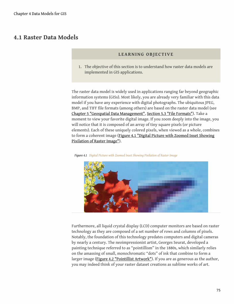
The raster data model is widely used in applications ranging far beyond geographicinformation systems (GISs). Most likely, you are already very familiar with this datamodel if you have any experience with digital photographs. The ubiquitous JPEG,BMP, and TIFF file formats (among others) are based on the raster data model (seeChapter 5 "Geospatial Data Management", Section 5.3 "File Formats"). Take amoment to view your favorite digital image. If you zoom deeply into the image, youwill notice that it is composed of an array of tiny square pixels (or pictureelements). Each of these uniquely colored pixels, when viewed as a whole, combinesto form a coherent image (Figure 4.1 "Digital Picture with Zoomed Inset ShowingPixilation of Raster Image").

Figure 4.1 Digital Picture with Zoomed Inset Showing Pixilation of Raster Image

Furthermore, all liquid crystal display (LCD) computer monitors are based on rastertechnology as they are composed of a set number of rows and columns of pixels.Notably, the foundation of this technology predates computers and digital camerasby nearly a century. The neoimpressionist artist, Georges Seurat, developed apainting technique referred to as “pointillism” in the 1880s, which similarly relieson the amassing of small, monochromatic “dots” of ink that combine to form alarger image (Figure 4.2 "Pointillist Artwork"). If you are as generous as the author,you may indeed think of your raster dataset creations as sublime works of art.

Chapter 4 Data Models for GIS

75

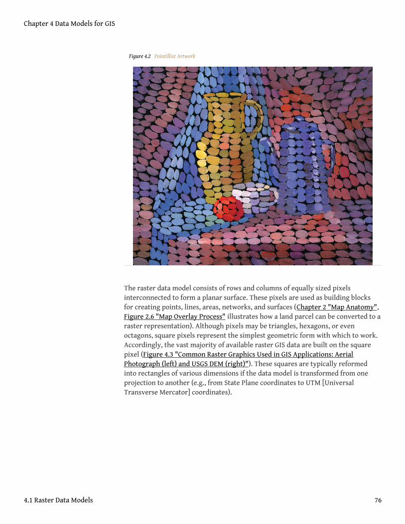
Figure 4.2 Pointillist Artwork

The raster data model consists of rows and columns of equally sized pixelsinterconnected to form a planar surface. These pixels are used as building blocksfor creating points, lines, areas, networks, and surfaces (Chapter 2 "Map Anatomy",Figure 2.6 "Map Overlay Process" illustrates how a land parcel can be converted to araster representation). Although pixels may be triangles, hexagons, or evenoctagons, square pixels represent the simplest geometric form with which to work.Accordingly, the vast majority of available raster GIS data are built on the squarepixel (Figure 4.3 "Common Raster Graphics Used in GIS Applications: AerialPhotograph (left) and USGS DEM (right)"). These squares are typically reformedinto rectangles of various dimensions if the data model is transformed from oneprojection to another (e.g., from State Plane coordinates to UTM [UniversalTransverse Mercator] coordinates).

Chapter 4 Data Models for GIS

4.1 Raster Data Models 76

Figure 4.3 Common Raster Graphics Used in GIS Applications: Aerial Photograph (left) and USGS DEM (right)

Source: Data available from U.S. Geological Survey, Earth Resources Observation and Science (EROS) Center, SiouxFalls, SD.

Because of the reliance on a uniform series of square pixels, the raster data model isreferred to as a grid-based system. Typically, a single data value will be assigned toeach grid locale. Each cell in a raster carries a single value, which represents thecharacteristic of the spatial phenomenon at a location denoted by its row andcolumn. The data type for that cell value can be either integer or floating-point(Chapter 5 "Geospatial Data Management", Section 5.1 "Geographic DataAcquisition"). Alternatively, the raster graphic can reference a databasemanagement system wherein open-ended attribute tables can be used to associatemultiple data values to each pixel. The advance of computer technology has madethis second methodology increasingly feasible as large datasets are no longerconstrained by computer storage issues as they were previously.

The raster model will average all values within a given pixel to yield a single value.Therefore, the more area covered per pixel, the less accurate the associated datavalues. The area covered by each pixel determines the spatial resolution1 of theraster model from which it is derived. Specifically, resolution is determined bymeasuring one side of the square pixel. A raster model with pixels representing 10m by 10 m (or 100 square meters) in the real world would be said to have a spatialresolution of 10 m; a raster model with pixels measuring 1 km by 1 km (1 squarekilometer) in the real world would be said to have a spatial resolution of 1 km; andso forth.1. The smallest distance between

two adjacent features that canbe detected in an image.

Chapter 4 Data Models for GIS

4.1 Raster Data Models 77

Care must be taken when determining the resolution of a raster because using anoverly coarse pixel resolution will cause a loss of information, whereas using overlyfine pixel resolution will result in significant increases in file size and computerprocessing requirements during display and/or analysis. An effective pixelresolution will take both the map scale and the minimum mapping unit of the otherGIS data into consideration. In the case of raster graphics with coarse spatialresolution, the data values associated with specific locations are not necessarilyexplicit in the raster data model. For example, if the location of telephone poleswere mapped on a coarse raster graphic, it would be clear that the entire cell wouldnot be filled by the pole. Rather, the pole would be assumed to be locatedsomewhere within that cell (typically at the center).

Imagery employing the raster data model must exhibit several properties. First,each pixel must hold at least one value, even if that data value is zero. Furthermore,if no data are present for a given pixel, a data value placeholder must be assigned tothis grid cell. Often, an arbitrary, readily identifiable value (e.g., −9999) will beassigned to pixels for which there is no data value. Second, a cell can hold anyalphanumeric index that represents an attribute. In the case of quantitativedatasets, attribute assignation is fairly straightforward. For example, if a rasterimage denotes elevation, the data values for each pixel would be some indication ofelevation, usually in feet or meters. In the case of qualitative datasets, data valuesare indices that necessarily refer to some predetermined translational rule. In thecase of a land-use/land-cover raster graphic, the following rule may be applied: 1 =grassland, 2 = agricultural, 3 = disturbed, and so forth (Figure 4.4 "Land-Use/Land-Cover Raster Image"). The third property of the raster data model is that points andlines “move” to the center of the cell. As one might expect, if a 1 km resolutionraster image contains a river or stream, the location of the actual waterway withinthe “river” pixel will be unclear. Therefore, there is a general assumption that allzero-dimensional (point) and one-dimensional (line) features will be located towardthe center of the cell. As a corollary, the minimum width for any line feature mustnecessarily be one cell regardless of the actual width of the feature. If it is not, thefeature will not be represented in the image and will therefore be assumed to beabsent.

Chapter 4 Data Models for GIS

4.1 Raster Data Models 78

Figure 4.4 Land-Use/Land-Cover Raster Image

Source: Data available from U.S. Geological Survey, Earth Resources Observation and Science (EROS) Center, SiouxFalls, SD.

Several methods exist for encoding raster data from scratch. Three of these modelsare as follows:

1. Cell-by-cell raster encoding2. This minimally intensive methodencodes a raster by creating records for each cell value by row andcolumn (Figure 4.5 "Cell-by-Cell Encoding of Raster Data"). Thismethod could be thought of as a large spreadsheet wherein each cell ofthe spreadsheet represents a pixel in the raster image. This method isalso referred to as “exhaustive enumeration.”

2. Run-length raster encoding3. This method encodes cell values in runsof similarly valued pixels and can result in a highly compressed imagefile (Figure 4.6 "Run-Length Encoding of Raster Data"). The run-lengthencoding method is useful in situations where large groups ofneighboring pixels have similar values (e.g., discrete datasets such asland use/land cover or habitat suitability) and is less useful where

2. A minimally intensive methodto encode a raster image bycreating unique records foreach cell value by row andcolumn. This method is alsoreferred to as “exhaustiveenumeration.”

3. A method to encode rasterimages by employing runs ofsimilarly valued pixels.

Chapter 4 Data Models for GIS

4.1 Raster Data Models 79

neighboring pixel values vary widely (e.g., continuous datasets such aselevation or sea-surface temperatures).

3. Quad-tree raster encoding4. This method divides a raster into ahierarchy of quadrants that are subdivided based on similarly valuedpixels (Figure 4.7 "Quad-Tree Encoding of Raster Data"). The division ofthe raster stops when a quadrant is made entirely from cells of thesame value. A quadrant that cannot be subdivided is called a “leafnode.”

Figure 4.5 Cell-by-Cell Encoding of Raster Data

4. A method used to encoderaster images by dividing theraster into a hierarchy ofquadrants that are subdividedbased on similarly valuedpixels.

Chapter 4 Data Models for GIS

4.1 Raster Data Models 80

Figure 4.6 Run-Length Encoding of Raster Data

Chapter 4 Data Models for GIS

4.1 Raster Data Models 81

Figure 4.7 Quad-Tree Encoding of Raster Data

Advantages/Disadvantages of the Raster Model

The use of a raster data model confers many advantages. First, the technologyrequired to create raster graphics is inexpensive and ubiquitous. Nearly everyonecurrently owns some sort of raster image generator, namely a digital camera, andfew cellular phones are sold today that don’t include such functionality. Similarly, aplethora of satellites are constantly beaming up-to-the-minute raster graphics toscientific facilities across the globe (Chapter 5 "Geospatial Data Management",Section 5.3 "File Formats"). These graphics are often posted online for private and/or public use, occasionally at no cost to the user.

Additional advantages of raster graphics are the relative simplicity of theunderlying data structure. Each grid location represented in the raster imagecorrelates to a single value (or series of values if attributes tables are included). Thissimple data structure may also help explain why it is relatively easy to performoverlay analyses on raster data (for more on overlay analyses, see Chapter 7"Geospatial Analysis I: Vector Operations", Section 7.1 "Single Layer Analysis"). Thissimplicity also lends itself to easy interpretation and maintenance of the graphics,relative to its vector counterpart.

Chapter 4 Data Models for GIS

4.1 Raster Data Models 82

Despite the advantages, there are also several disadvantages to using the raster datamodel. The first disadvantage is that raster files are typically very large.Particularly in the case of raster images built from the cell-by-cell encodingmethodology, the sheer number of values stored for a given dataset result inpotentially enormous files. Any raster file that covers a large area and hassomewhat finely resolved pixels will quickly reach hundreds of megabytes in size ormore. These large files are only getting larger as the quantity and quality of rasterdatasets continues to keep pace with quantity and quality of computer resourcesand raster data collectors (e.g., digital cameras, satellites).

A second disadvantage of the raster model is that the output images are less“pretty” than their vector counterparts. This is particularly noticeable when theraster images are enlarged or zoomed (refer to Figure 4.1 "Digital Picture withZoomed Inset Showing Pixilation of Raster Image"). Depending on how far onezooms into a raster image, the details and coherence of that image will quickly belost amid a pixilated sea of seemingly randomly colored grid cells.

The geometric transformations that arise during map reprojection efforts can causeproblems for raster graphics and represent a third disadvantage to using the rasterdata model. As described in Chapter 2 "Map Anatomy", Section 2.2 "Map Scale,Coordinate Systems, and Map Projections", changing map projections will alter thesize and shape of the original input layer and frequently result in the loss oraddition of pixels (White 2006).White, D. 2006. “Display of Pixel Loss and Replicationin Reprojecting Raster Data from the Sinusoidal Projection.” Geocarto International 21(2): 19–22. These alterations will result in the perfect square pixels of the inputlayer taking on some alternate rhomboidal dimensions. However, the problem islarger than a simple reformation of the square pixel. Indeed, the reprojection of araster image dataset from one projection to another brings change to pixel valuesthat may, in turn, significantly alter the output information (Seong 2003).Seong, J.C. 2003. “Modeling the Accuracy of Image Data Reprojection.” International Journal ofRemote Sensing 24 (11): 2309–21.

The final disadvantage of using the raster data model is that it is not suitable forsome types of spatial analyses. For example, difficulties arise when attempting tooverlay and analyze multiple raster graphics produced at differing scales and pixelresolutions. Combining information from a raster image with 10 m spatialresolution with a raster image with 1 km spatial resolution will most likely producenonsensical output information as the scales of analysis are far too disparate toresult in meaningful and/or interpretable conclusions. In addition, some networkand spatial analyses (i.e., determining directionality or geocoding) can beproblematic to perform on raster data.

Chapter 4 Data Models for GIS

4.1 Raster Data Models 83

KEY TAKEAWAYS

• Raster data are derived from a grid-based system of contiguous cellscontaining specific attribute information.

• The spatial resolution of a raster dataset represents a measure of theaccuracy or detail of the displayed information.

• The raster data model is widely used by non-GIS technologies such asdigital cameras/pictures and LCD monitors.

• Care should be taken to determine whether the raster or vector datamodel is best suited for your data and/or analytical needs.

EXERCISES

1. Examine a digital photo you have taken recently. Can you estimate itsspatial resolution?

2. If you were to create a raster data file showing the major land-use typesin your county, which encoding method would you use? What methodwould you use if you were to encode a map of the major waterways inyour county? Why?

Chapter 4 Data Models for GIS

4.1 Raster Data Models 84

4.2 Vector Data Models

LEARNING OBJECTIVE

1. The objective of this section is to understand how vector data modelsare implemented in GIS applications.

In contrast to the raster data model is the vector data model. In this model, space isnot quantized into discrete grid cells like the raster model. Vector data models usepoints and their associated X, Y coordinate pairs to represent the vertices of spatialfeatures, much as if they were being drawn on a map by hand (Aronoff1989).Aronoff, S. 1989. Geographic Information Systems: A Management Perspective.Ottawa, Canada: WDL Publications. The data attributes of these features are thenstored in a separate database management system. The spatial information and theattribute information for these models are linked via a simple identificationnumber that is given to each feature in a map.

Three fundamental vector types exist in geographic information systems (GISs):points, lines, and polygons (Figure 4.8 "Points, Lines, and Polygons"). Points5 arezero-dimensional objects that contain only a single coordinate pair. Points aretypically used to model singular, discrete features such as buildings, wells, powerpoles, sample locations, and so forth. Points have only the property of location.Other types of point features include the node6 and the vertex7. Specifically, a pointis a stand-alone feature, while a node is a topological junction representing acommon X, Y coordinate pair between intersecting lines and/or polygons. Verticesare defined as each bend along a line or polygon feature that is not the intersectionof lines or polygons.

5. A zero-dimensional objectcontaining a single coordinatepair. In a GIS, points have onlythe property of location.

6. The intersection points wheretwo or more arcs meet.

7. A corner or a point where linesmeet.

Chapter 4 Data Models for GIS

85

Figure 4.8 Points, Lines, and Polygons

Points can be spatially linked to form more complex features. Lines8 are one-dimensional features composed of multiple, explicitly connected points. Lines areused to represent linear features such as roads, streams, faults, boundaries, and soforth. Lines have the property of length. Lines that directly connect two nodes aresometimes referred to as chains, edges, segments, or arcs9.

Polygons10 are two-dimensional features created by multiple lines that loop back tocreate a “closed” feature. In the case of polygons, the first coordinate pair (point)on the first line segment is the same as the last coordinate pair on the last linesegment. Polygons are used to represent features such as city boundaries, geologicformations, lakes, soil associations, vegetation communities, and so forth. Polygonshave the properties of area and perimeter. Polygons are also called areas11.

Vector Data Models Structures

Vector data models can be structured many different ways. We will examine two ofthe more common data structures here. The simplest vector data structure is calledthe spaghetti data model12 (Dangermond 1982).Dangermond, J. 1982. “AClassification of Software Components Commonly Used in Geographic Information

8. A one-dimensional objectcomposed of multiple,explicitly connected points.Lines have the property oflength. Also called an “arc.”

9. A one-dimensional objectcomposed of multiple,explicitly connected points.Lines have the property oflength. Also called a “line.”

10. A two-dimensional featurecreated from multiple linesthat loop back to create a“closed” feature. Polygonshave the properties of area andperimeter. Also called “areas.”

11. A two-dimensional featurecreated from multiple linesthat loop back to create a“closed” feature. Areas havethe properties of area andperimeter. Also called“polygons.”

12. A data model in which eachpoint, line, and/or polygonfeature is represented as astring of X, Y coordinate pairswith no inherent structure.

Chapter 4 Data Models for GIS

4.2 Vector Data Models 86

Systems.” In Proceedings of the U.S.-Australia Workshop on the Design and Implementationof Computer-Based Geographic Information Systems, 70–91. Honolulu, HI. In thespaghetti model, each point, line, and/or polygon feature is represented as a stringof X, Y coordinate pairs (or as a single X, Y coordinate pair in the case of a vectorimage with a single point) with no inherent structure (Figure 4.9 "Spaghetti DataModel"). One could envision each line in this model to be a single strand ofspaghetti that is formed into complex shapes by the addition of more and morestrands of spaghetti. It is notable that in this model, any polygons that lie adjacentto each other must be made up of their own lines, or stands of spaghetti. In otherwords, each polygon must be uniquely defined by its own set of X, Y coordinatepairs, even if the adjacent polygons share the exact same boundary information.This creates some redundancies within the data model and therefore reducesefficiency.

Figure 4.9 Spaghetti Data Model

Despite the location designations associated with each line, or strand of spaghetti,spatial relationships are not explicitly encoded within the spaghetti model; rather,they are implied by their location. This results in a lack of topological information,which is problematic if the user attempts to make measurements or analysis. Thecomputational requirements, therefore, are very steep if any advanced analyticaltechniques are employed on vector files structured thusly. Nevertheless, the simplestructure of the spaghetti data model allows for efficient reproduction of maps andgraphics as this topological information is unnecessary for plotting and printing.

In contrast to the spaghetti data model, the topological data model13 ischaracterized by the inclusion of topological information within the dataset, as thename implies. Topology14 is a set of rules that model the relationships between

13. A data model characterized bythe inclusion of topology.

14. A set of rules that models therelationship betweenneighboring points, lines, andpolygons and determines howthey share geometry. Topologyis also concerned withpreserving spatial propertieswhen the forms are bent,stretched, or placed undersimilar geometrictransformation.

Chapter 4 Data Models for GIS

4.2 Vector Data Models 87

neighboring points, lines, and polygons and determines how they share geometry.For example, consider two adjacent polygons. In the spaghetti model, the sharedboundary of two neighboring polygons is defined as two separate, identical lines.The inclusion of topology into the data model allows for a single line to representthis shared boundary with an explicit reference to denote which side of the linebelongs with which polygon. Topology is also concerned with preserving spatialproperties when the forms are bent, stretched, or placed under similar geometrictransformations, which allows for more efficient projection and reprojection of mapfiles.

Three basic topological precepts that are necessary to understand the topologicaldata model are outlined here. First, connectivity15 describes the arc-node topologyfor the feature dataset. As discussed previously, nodes are more than simple points.In the topological data model, nodes are the intersection points where two or morearcs meet. In the case of arc-node topology, arcs have both a from-node (i.e.,starting node) indicating where the arc begins and a to-node (i.e., ending node)indicating where the arc ends (Figure 4.10 "Arc-Node Topology"). In addition,between each node pair is a line segment, sometimes called a link, which has itsown identification number and references both its from-node and to-node. InFigure 4.10 "Arc-Node Topology", arcs 1, 2, and 3 all intersect because they sharenode 11. Therefore, the computer can determine that it is possible to move alongarc 1 and turn onto arc 3, while it is not possible to move from arc 1 to arc 5, as theydo not share a common node.

Figure 4.10 Arc-Node Topology

15. The topological property oflines sharing a common node.

Chapter 4 Data Models for GIS

4.2 Vector Data Models 88

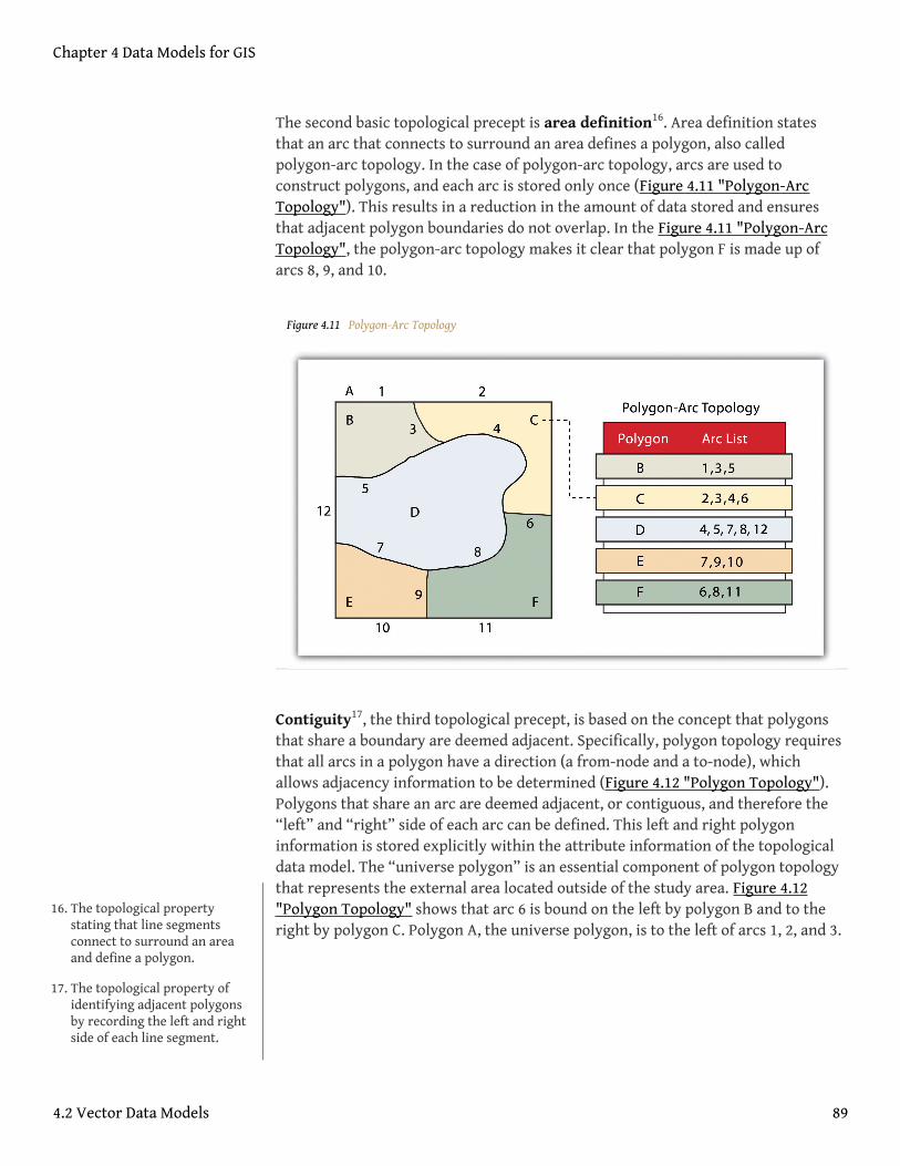
The second basic topological precept is area definition16. Area definition statesthat an arc that connects to surround an area defines a polygon, also calledpolygon-arc topology. In the case of polygon-arc topology, arcs are used toconstruct polygons, and each arc is stored only once (Figure 4.11 "Polygon-ArcTopology"). This results in a reduction in the amount of data stored and ensuresthat adjacent polygon boundaries do not overlap. In the Figure 4.11 "Polygon-ArcTopology", the polygon-arc topology makes it clear that polygon F is made up ofarcs 8, 9, and 10.

Figure 4.11 Polygon-Arc Topology

Contiguity17, the third topological precept, is based on the concept that polygonsthat share a boundary are deemed adjacent. Specifically, polygon topology requiresthat all arcs in a polygon have a direction (a from-node and a to-node), whichallows adjacency information to be determined (Figure 4.12 "Polygon Topology").Polygons that share an arc are deemed adjacent, or contiguous, and therefore the“left” and “right” side of each arc can be defined. This left and right polygoninformation is stored explicitly within the attribute information of the topologicaldata model. The “universe polygon” is an essential component of polygon topologythat represents the external area located outside of the study area. Figure 4.12"Polygon Topology" shows that arc 6 is bound on the left by polygon B and to theright by polygon C. Polygon A, the universe polygon, is to the left of arcs 1, 2, and 3.

16. The topological propertystating that line segmentsconnect to surround an areaand define a polygon.

17. The topological property ofidentifying adjacent polygonsby recording the left and rightside of each line segment.

Chapter 4 Data Models for GIS

4.2 Vector Data Models 89

Figure 4.12 Polygon Topology

Topology allows the computer to rapidly determine and analyze the spatialrelationships of all its included features. In addition, topological information isimportant because it allows for efficient error detection within a vector dataset. Inthe case of polygon features, open or unclosed polygons, which occur when an arcdoes not completely loop back upon itself, and unlabeled polygons, which occurwhen an area does not contain any attribute information, violate polygon-arctopology rules. Another topological error found with polygon features is thesliver18. Slivers occur when the shared boundary of two polygons do not meetexactly (Figure 4.13 "Common Topological Errors").

In the case of line features, topological errors occur when two lines do not meetperfectly at a node. This error is called an “undershoot” when the lines do notextend far enough to meet each other and an “overshoot” when the line extendsbeyond the feature it should connect to (Figure 4.13 "Common Topological Errors").The result of overshoots and undershoots is a “dangling node” at the end of theline. Dangling nodes aren’t always an error, however, as they occur in the case ofdead-end streets on a road map.

18. A narrow gap formed when theshared boundary of twopolygons do not meet exactly.

Chapter 4 Data Models for GIS

4.2 Vector Data Models 90

Figure 4.13 Common Topological Errors

Many types of spatial analysis require the degree of organization offered bytopologically explicit data models. In particular, network analysis (e.g., finding thebest route from one location to another) and measurement (e.g., finding the lengthof a river segment) relies heavily on the concept of to- and from-nodes and uses thisinformation, along with attribute information, to calculate distances, shortestroutes, quickest routes, and so forth. Topology also allows for sophisticatedneighborhood analysis such as determining adjacency, clustering, nearestneighbors, and so forth.

Now that the basics of the concepts of topology have been outlined, we can begin tobetter understand the topological data model. In this model, the node acts as morethan just a simple point along a line or polygon. The node represents the point ofintersection for two or more arcs. Arcs may or may not be looped into polygons.Regardless, all nodes, arcs, and polygons are individually numbered. Thisnumbering allows for quick and easy reference within the data model.

Advantages/Disadvantages of the Vector Model

In comparison with the raster data model, vector data models tend to be betterrepresentations of reality due to the accuracy and precision of points, lines, andpolygons over the regularly spaced grid cells of the raster model. This results invector data tending to be more aesthetically pleasing than raster data.

Chapter 4 Data Models for GIS

4.2 Vector Data Models 91

Vector data also provides an increased ability to alter the scale of observation andanalysis. As each coordinate pair associated with a point, line, and polygonrepresents an infinitesimally exact location (albeit limited by the number ofsignificant digits and/or data acquisition methodologies), zooming deep into avector image does not change the view of a vector graphic in the way that it does araster graphic (see Figure 4.1 "Digital Picture with Zoomed Inset Showing Pixilationof Raster Image").

Vector data tend to be more compact in data structure, so file sizes are typicallymuch smaller than their raster counterparts. Although the ability of moderncomputers has minimized the importance of maintaining small file sizes, vectordata often require a fraction the computer storage space when compared to rasterdata.

The final advantage of vector data is that topology is inherent in the vector model.This topological information results in simplified spatial analysis (e.g., errordetection, network analysis, proximity analysis, and spatial transformation) whenusing a vector model.

Alternatively, there are two primary disadvantages of the vector data model. First,the data structure tends to be much more complex than the simple raster datamodel. As the location of each vertex must be stored explicitly in the model, thereare no shortcuts for storing data like there are for raster models (e.g., the run-length and quad-tree encoding methodologies).

Second, the implementation of spatial analysis can also be relatively complicateddue to minor differences in accuracy and precision between the input datasets.Similarly, the algorithms for manipulating and analyzing vector data are complexand can lead to intensive processing requirements, particularly when dealing withlarge datasets.

Chapter 4 Data Models for GIS

4.2 Vector Data Models 92

KEY TAKEAWAYS

• Vector data utilizes points, lines, and polygons to represent the spatialfeatures in a map.

• Topology is an informative geospatial property that describes theconnectivity, area definition, and contiguity of interrelated points, lines,and polygon.

• Vector data may or may not be topologically explicit, depending on thefile’s data structure.

• Care should be taken to determine whether the raster or vector datamodel is best suited for your data and/or analytical needs.

EXERCISES

1. What vector type (point, line, or polygon) best represents the followingfeatures: state boundaries, telephone poles, buildings, cities, streamnetworks, mountain peaks, soil types, flight tracks? Which of thesefeatures can be represented by multiple vector types? What conditionsmight lead you choose one vector type over another?

2. Draw a point, line, and polygon feature on a simple Cartesian coordinatesystem. From this drawing, create a spaghetti data model thatapproximates the shapes shown therein.

3. Draw three adjacent polygons on a simple Cartesian coordinate system.From this drawing, create a topological data model that incorporatesarc-node, polygon-arc, and polygon topology.

Chapter 4 Data Models for GIS

4.2 Vector Data Models 93

4.3 Satellite Imagery and Aerial Photography

LEARNING OBJECTIVE

1. The objective of this section is to understand how satellite imagery andaerial photography are implemented in GIS applications.

A wide variety of satellite imagery and aerial photography is available for use ingeographic information systems (GISs). Although these products are basically rastergraphics, they are substantively different in their usage within a GIS. Satelliteimagery and aerial photography provide important contextual information for aGIS and are often used to conduct heads-up digitizing (Chapter 5 "Geospatial DataManagement", Section 5.1.4 "Secondary Data Capture") whereby features from theimage are converted into vector datasets.

Satellite Imagery

Remotely sensed satellite imagery is becoming increasingly common as satellitesequipped with technologically advanced sensors are continually being sent intospace by public agencies and private companies around the globe. Satellites areused for applications such as military and civilian earth observation,communication, navigation, weather, research, and more. Currently, more than3,000 satellites have been sent to space, with over 2,500 of them originating fromRussia and the United States. These satellites maintain different altitudes,inclinations, eccentricities, synchronies, and orbital centers, allowing them toimage a wide variety of surface features and processes (Figure 4.14 "SatellitesOrbiting the Earth").

Chapter 4 Data Models for GIS

94

Figure 4.14 Satellites Orbiting the Earth

Satellites can be active or passive. Active satellites19 make use of remote sensorsthat detect reflected responses from objects that are irradiated from artificiallygenerated energy sources. For example, active sensors such as radars emit radiowaves, laser sensors emit light waves, and sonar sensors emit sound waves. In allcases, the sensor emits the signal and then calculates the time it takes for thereturned signal to “bounce” back from some remote feature. Knowing the speed ofthe emitted signal, the time delay from the original emission to the return can beused to calculate the distance to the feature.

Passive satellites20, alternatively, make use of sensors that detect the reflected oremitted electromagnetic radiation from natural sources. This natural source istypically the energy from the sun, but other sources can be imaged as well, such asmagnetism and geothermal activity. Using an example we’ve all experienced, takinga picture with a flash-enabled camera would be active remote sensing, while using acamera without a flash (i.e., relying on ambient light to illuminate the scene) wouldbe passive remote sensing.

The quality and quantity of satellite imagery is largely determined by theirresolution. There are four types of resolution that characterize any particularremote sensor (Campbell 2002).Campbell, J. B. 2002. Introduction to Remote Sensing.New York: Guilford Press. The spatial resolution21 of a satellite image, as describedpreviously in the raster data model section (Section 4.1 "Raster Data Models"), is a

19. Remote sensors that detectreflected responses fromobjects that are irradiated fromartificially generated energysources.

20. Remote sensors that detect thereflected or emittedelectromagnetic radiation fromnatural sources.

21. The smallest distance betweentwo adjacent features that canbe detected in an image.

Chapter 4 Data Models for GIS

4.3 Satellite Imagery and Aerial Photography 95

direct representation of the ground coverage for each pixel shown in the image. If asatellite produces imagery with a 10 m resolution, the corresponding groundcoverage for each of those pixels is 10 m by 10 m, or 100 square meters on theground. Spatial resolution is determined by the sensors’ instantaneous field of view(IFOV). The IFOV is essentially the ground area through which the sensor isreceiving the electromagnetic radiation signal and is determined by height andangle of the imaging platform.

Spectral resolution22 denotes the ability of the sensor to resolve wavelengthintervals, also called bands, within the electromagnetic spectrum. The spectralresolution is determined by the interval size of the wavelengths and the number ofintervals being scanned. Multispectral and hyperspectral sensors are those sensorsthat can resolve a multitude of wavelengths intervals within the spectrum. Forexample, the IKONOS satellite resolves images for bands at the blue (445–516 nm),green (506–95 nm), red (632–98 nm), and near-infrared (757–853 nm) wavelengthintervals on its 4-meter multispectral sensor.

Temporal resolution23 is the amount of time between each image collection periodand is determined by the repeat cycle of the satellite’s orbit. Temporal resolutioncan be thought of as true-nadir or off-nadir. Areas considered true-nadir are thoselocated directly beneath the sensor while off-nadir areas are those that are imagedobliquely. In the case of the IKONOS satellite, the temporal resolution is 3 to 5 daysfor off-nadir imaging and 144 days for true-nadir imaging.

The fourth and final type of resolution, radiometric resolution24, refers to thesensitivity of the sensor to variations in brightness and specifically denotes thenumber of grayscale levels that can be imaged by the sensor. Typically, theavailable radiometric values for a sensor are 8-bit (yielding values that range from0–255 as 256 unique values or as 28 values); 11-bit (0–2,047); 12-bit (0–4,095); or16-bit (0–63,535) (see Chapter 5 "Geospatial Data Management", Section 5.1.1 "DataTypes" for more on bits). Landsat-7, for example, maintains 8-bit resolution for itsbands and can therefore record values for each pixel that range from 0 to 255.

Because of the technical constraints associated with satellite remote sensingsystems, there is a trade-off between these different types of resolution. Improvingone type of resolution often necessitates a reduction in one of the other types ofresolution. For example, an increase in spatial resolution is typically associatedwith a decrease in spectral resolution, and vice versa. Similarly, geostationarysatellites25 (those that circle the earth proximal to the equator once each day) yieldhigh temporal resolution but low spatial resolution, while sun-synchronoussatellites26 (those that synchronize a near-polar orbit of the sensor with the sun’sillumination) yield low temporal resolution while providing high spatial resolution.

22. The ability of a sensor toresolve wavelength intervals,also called bands, within theelectromagnetic spectrum.

23. The amount of time betweeneach image collection perioddetermined by the repeat cycleof a satellite’s orbit.

24. The sensitivity of a remotesensor to variations inbrightness.

25. Satellites that circle the earthproximal to the equator onceeach day.

26. Satellites that synchronize anear-polar orbit with the sun’sillumination.

Chapter 4 Data Models for GIS

4.3 Satellite Imagery and Aerial Photography 96

Although technological advances can generally improve the various resolutions ofan image, care must always be taken to ensure that the imagery you have chosen isadequate to the represent or model the geospatial features that are most importantto your study.

Aerial Photography

Aerial photography, like satellite imagery, represents a vast source of informationfor use in any GIS. Platforms for the hardware used to take aerial photographsinclude airplanes, helicopters, balloons, rockets, and so forth. While aerialphotography connotes images taken of the visible spectrum, sensors to measurebands within the nonvisible spectrum (e.g., ultraviolet, infrared, near-infrared) canalso be fixed to aerial sources. Similarly, aerial photography can be active or passiveand can be taken from vertical or oblique angles. Care must be taken with aerialphotographs as the sensors used to take the images are similar to cameras in theiruse of lenses. These lenses add a curvature to the images, which becomes morepronounced as one moves away from the center of the photo (Figure 4.15"Curvature Error Due to Lenticular Properties of Camera").

Figure 4.15 Curvature Error Due to Lenticular Properties of Camera

Chapter 4 Data Models for GIS

4.3 Satellite Imagery and Aerial Photography 97

Another source of potential error in an aerial photograph is relief displacement.This error arises from the three-dimensional aspect of terrain features and is seenas apparent leaning away of vertical objects from the center point of an aerialphotograph. To imagine this type of error, consider that a smokestack would looklike a doughnut if the viewing camera was directly above the feature. However, ifthis same smokestack was observed near the edge of the camera’s view, one couldobserve the sides of the smokestack. This error is frequently seen with trees andmultistory buildings and worsens with increasingly taller features.

Orthophotos27 are vertical photographs that have been geometrically “corrected”to remove the curvature and terrain-induced error from images (Figure 4.16"Orthophoto"). The most common orthophoto product is the digital ortho quarterquadrangle (DOQQ). DOQQs are available through the US Geological Survey (USGS),who began producing these images from their library of 1:40,000-scale NationalAerial Photography Program photos. These images can be obtained in eithergrayscale or color with 1-meter spatial resolution and 8-bit radiometric resolution.As the name suggests, these images cover a quarter of a USGS 7.5 minutequadrangle, which equals an approximately 25 square mile area. Included withthese photos is an additional 50 to 300-meter edge around the photo that allowsusers to mosaic many DOQQs into a single, continuous image. These DOQQs are idealfor use in a GIS as background display information, for data editing, and for heads-up digitizing.

27. Vertical photographs that havebeen geometrically “corrected”to remove the curvature andterrain-induced error fromimages.

Chapter 4 Data Models for GIS

4.3 Satellite Imagery and Aerial Photography 98

Figure 4.16 Orthophoto

Source: Data available from U.S. Geological Survey, Earth Resources Observation and Science (EROS) Center, SiouxFalls, SD.

KEY TAKEAWAYS

• Satellite imagery is a common tool for GIS mapping applications as thisdata becomes increasingly available due to ongoing technologicaladvances.

• Satellite imagery can be passive or active.• The four types of resolution associated with satellite imagery are spatial,

spectral, temporal, and radiometric.• Vertical and oblique aerial photographs provide valuable baseline

information for GIS applications.

Chapter 4 Data Models for GIS

4.3 Satellite Imagery and Aerial Photography 99

EXERCISE

1. Go to the EarthExplorer website (http://edcsns17.cr.usgs.gov/EarthExplorer) and download two satellite images of the area in whichyou reside. What are the different spatial, spectral, temporal, andradiometric resolutions for these two images? Do these satellitesprovide active or passive imagery (or both)? Are they geostationary orsun-synchronous?

Chapter 4 Data Models for GIS

4.3 Satellite Imagery and Aerial Photography 100