________________________________________________________________________

Theory and Practice of Biomolecular Modelling & Simulation

by B. Jayaram1 and D.L. Beveridge2

1 Deptt. of Chemistry, Indian Institute of Technology, New Delhi, India 2 Deptt. of Chemistry, Wesleyan University, Chemistry and †Molecular Biophysics Program, Wesleyan University, Middletown, CT 06459

________________________________________________________________________ Contents 1. Introduction 1. 1. Potential Functions 1.2 Quantum Mechanical Basis 2. Structure & Dynamics 3. Thermodynamics 4. Rate Constants I. Introduction 1.1 Potential Functions Recall the ball and stick model of a 1,2-disubstituted ethane introduced at high-school level these days. Ideas related to hindered rotation around a single bond, the instability of an eclipsed conformation relative to its staggered analogue emerge in a visually telling manner. The balls of course represent atoms and the sticks the chemical bonds between atoms. A clash between two unconnected balls upon rotation around the axis of a stick, is interpreted as steric hindrance to rotation. This simple model provides a powerful tool to appreciate strain and stability associated with molecular conformations. It has been a valuable companion in synthetic and mechanistic organic chemistry and in other areas as well. In such a model, from the standpoint of intermolecular forces, there are no attractions between two unconnected atoms and no repulsions either, not even when the two atoms encounter each other - just that they cannot pass through each other. If this behaviour is to be formulated mathematically, one would say that the potential energy between two non-bonded atoms is zero for all distances greater than the sum of their radii and the energy goes to infinity if the distance is less than the above sum. This in the technical jargon is known as a hard sphere model which in a primitive way describes the interaction between two non-bonded atoms. The sticks which are not elastic imply that the force constants associated with the bonds and bond angles are infinitely large. A free rotation around a bond is indicative of a flat torsional energy surface. Some of these approximations can be easily removed. A soft sphere potential which includes van der Waals attractions and short range repulsions originating in Pauli’s forces can be employed, as with a (12,6) Lennard-Jones potential or a Buckingham potential (exp,6), in lieu of the hard sphere model. A coulombic potential can be added to this if the two atoms carry charges, fractional or full. Similarly, the force costants

1

associated with bond stretching and angle bending can be assigned more realistic values instead of infinities. The torsional energy surface can also be modified to represent reality more closely by introducing multiple minima indicating the conformational preferences of the molecule. Thus all the internal degrees of freedom of the molecule can be taken cognizance of. E k l l k V n

R r R r q q Dr

N

all bondsl o o n o

all dihedral anglesall bond angles

ij ij ij ij ij i j ijall non bondedpairs

( ) ) ( ) ) ( ) ) ( cos ( )

[ ( / ) ( / ) ( / )]

X = − + − + +

− +

∑ )−∑∑

∑−

( ( (

+ (1)

12

12

12

2 2

12 6

1

2

θ θ θ ω ω

ε

In the above equation, the first term describes the penalty for bond stretch from its equilibrium value. kl is the force constant for bond stretch and lo the equilibrium bond length. The second term denotes the energy penalty for deforming the bond angle. θo is the equilibrium value for the bond angle and kθ the corresponding force constant. Both first and second terms are harmonic (i.e. Hooke’s law type) functions. Cross terms of the stretch-bend genre can also be added if required. The third term, a Fourier series representation, quantifies the energy as a function of the dihedral angle ω. Vn is the rotational barrier height, n is the periodicity of rotation, ωo is the reference angle where the torsional energy is maximum. This function (expressed further as a sum of different terms with n >1 in the Fourier series) captures the multiple energy minima of varying heights usually seen with dihedral angle variations. The non-bonded interactions are taken care of by the last term. εij is the well depth, Rij is the minimum energy interaction distance, qi and qj are the partial charges on atoms i and j, rij is the distance between them and D is a dielectric function. The consequence of all these refinements (equation 1) is that the ball and stick model hops out of our hands to become a more accurate molecular model easier handled by a computer. Qualitative arguments on stability and reactivity turn quantitative. Just as the original ball and stick model, computer modelling is but a tool to help interpret experiment at an atomic level, to suggest new experiments without the ordeals of the hit and trial approach and to generate new knowledge on the behaviour of the molecular system whereever experiments are difficult to perform. The current day computational research in the realm of biomolecules is concerned with developing a molecular view of stability and recognition based on the laws of physics. This is an energy-based approach. Other approaches profiting from computational techniques involving artificial intelligence, distance geometry, computer graphics etc. have also found fruitful applications in deciphering biomolecular structure and function such as in modelling protein structures and in NMR structural refinements. The main focus of the following discussion will be on energy-based approaches. A potential function [1] (equation 1) is a prescription for computing the energy of the molecular system if the cartesian coordinates (i. e. configuration XN) of all the atoms / ions / particles of the system are specified. The energy computed is often referred to as single point energy, i. e. the energy of the point XN in the configuration space of the molecular system. A force field comprises a potential function together with a listing of all the parameters required for the calculation of energy and forces, such as the force

2

constants, the equilibrium values for the internal degrees of freedom each considered in isolation, the partial atomic charges on each of the atoms in varying chemical environments etc.. The parameters come from extensive and careful calibrations against experiment or rigorous quantum mechanical calculations. AMBER [2], CHARMM [3], CVFF, CFF-91 & CFF-95 [4], ECEPP [5], GROMOS [6], MMx (x=1,2,3) [7], OPLS [8] are some of the popular force fields in vogue today. (Names such as AMBER and GROMOS are also used for a suite of programs which perform modelling and simulations.) Each of the above force fields has undergone considerable improvements over the years with a significant increase in accuracy and reliability of the computational predictions. An alternative to the potential function approach is to solve the Schrodinger equation for the system but this becomes computationally prohibitive as the system size increases. The choice between molecular mechanics and quantum mechanics rests on the system size and the level of rigour required in representing the system. For biomolecular systems consisting of 103-104 atoms, the former is the obvious choice although whenever a chemical bond is formed or an electron transfer occurs a quantum treatment in some form or another is indispensable. In energy minimization (EM) protocols, the objective is to arrive at a structure that has the minimum most energy. Several methods such as the steepest descent, conjugate gradient, Newton-Raphson method have been proposed to accomplish this task [1]. Starting with an arbitrary structure one often ends up with the nearest energy minimum in the configuration space of the molecule. Global energy minimum is elusive but is reachable for small systems by an intelligent design of a series of minimizations. This - a structure with minimum most energy - is often the goal of molecular modelling exercises. This is supplemented with the hypothesis that the lower the energy the more stable is the mechanical system. Most of the questions related to structure and function can be converted to energy related problems. Conformational analysis is a stability problem which involves mapping the energy as a function of the internal coordinates of the molecule. The effect of a mutation on the stability of a protein can be converted into a problem seeking the minimum energy structures of the system before and after the mutation followed by a computation of the energy difference. The relative binding efficacy of a series of ligands to a receptor is a recognition problem. The minimum energy structure of the receptor-ligand complex with each ligand is generated. The binding energy is then computed as ∆Ebinding = Ecomplex - (Ereceptor + Eligand). This allows an ordering of the ligands based on the energetics which hopefully correlates with the binding constant data (∆Go = - R T ln K; ∆Go is the change in the standard free energy, R is the gas constant, T the absolute temperature and K the equilibrium constant). A serious theoretical limitation of the energy minimization studies besides the difficulty in attaining the global minimum, is the lack of contact with thermodynamics and the consequent loss of correspondence with experiment. This notwithstanding, energy minimization studies continue to be of considerable value providing qualitative insights into the problem on hand and prove to be decisive in favourable cases, especially where entropic effects and thermal averaging are expected to play only a minor role. Methods to compute heats of formation and entropies via a normal mode analysis have also been developed [1]. Molecular mechanics calculations are employed routinely for investigating structure-activity relationships particularly in the area of drug design.

3

The connection with thermodynamics is established via an ensemble averaging (as in Monte Carlo method) or a time averaging (as in molecular dynamics method) of the energies of all the configurations accessible to the system under specified conditions (constant temperature, volume and number of particles for instance). This gives the average internal energy U. U = <E(XN)> where angular brackets denote Boltzmann averages. This with a pressure volume correction gives the enthalpy (H = U + PV). A further addition of the entropic term results in the Gibbs free energy of the system (G = H - T S). Molecular simulations via Monte Carlo (MC) method (in which the configurations of the system are generated according to Boltzmann distribution in a stochastic approach) or molecular dynamics (MD) method (where new configurations of the system are generated by solving equations of motion in a deterministic approach) mimic the system at equilibrium and both structural and thermodynamic properties of the system become accessible. Besides these MD also yields dynamic properties. The MC method due to Metropolis et al. [9], the molecular dynamics studies of Alder and Wainright [10] on simple liquids, those of Rahman and Stillinger [11] on liquid water and the pioneering theoretical studies of Scheraga and coworkers [12] on proteins, influenced the course of events quite significantly. Molecular dynamics (MD) studies on BPTI in vacuo [13] and alanine dipeptide in water [14] constitute some of the significant early attempts to apply the MD technique to biomolecular systems. Parallel to this evolved the MC methodology as applied to aqueous solutions of biomolecules [15,16]. The last decade has seen a welcome explosion in the numerous extensions and improvements of the above methodologies as applied to biomolecular systems [17-23 and references therein] in several Laboratories all over the globe. Structure and conformation of biomolecules are sensitive to solvent and salt concentration. Modelling molecules under physiological conditions implies a consideration of the aqueous environment preferably along with the supporting electrolyte (145 mM NaCl for instance). The first step thus is to ensure that an accurate description of the structure and thermodynamics of solvent water is available. Several water models have been proposed, SPC [24] and TIP4P [25] being two of the popular choices. Simulations of aqueous solutions proceed via the solvation of biomolecule of interest with desired / sufficient number of explicit waters (TIP4P or any such water model) with their configurations, along with that of the biomolecule, generated by MD or MC simulations. Water organization around biomolecules has become an intense research area [26-28] with a growing theoretical evidence of its stabilizing influence and the concurrent experimental observations such as the identification of spine of hydration in the minor groove of a B-DNA crystal structure [29] and the observation that water trapped at the interface of two biomolecules (protein and DNA for instance) could contribute to specificity via water mediated hydrogen bonds [30] and via energetics of desolvation. Several methods of solvent analysis have been proposed of which the proximity criterion developed by Beveridge and coworkers [31], enables a quantification of the structure and energetics of solvent around multifunctional solutes, in a unique fashion, via quasi-component molecular distribution functions [32]. Salt effects can be included in a natural way in the simulations once the ion-water [33], ion-ion and ion-solute potential functions are available. The number of small ions considered is mostly restricted to maintaining electroneutrality in the solution and few simulations reported thus far could consider added salt effects. This is due to severe

4

convergence problems in simulations with ions and issues related to sampling. Thus methodologies exist at least in principle, to deal with the environmental (solvent and salt) effects on the stability of biomolecules. An outstanding problem of current interest to researchers in biomolecular area is that of molecular recognition. Protein folding is an intramolecular recognition problem and regulation of gene expression by certain proteins (protein-DNA recognition) is an intermolecular recognition problem. Also the environmental factors such as solvent activity and salt concentration exert a fine control on recognition. Two critical indices that a chemist desires out of a theoretical study of such events is the free energy of folding / binding and rates associated with these processes. Once the thermodynamic and kinetic parameters are specified, the focus shifts to an understanding of the origins of stability, spontaneity and speed at an atomic level. This is to help design molecules with altered stabilites and binding proclivities.. Theoretical tools available for biomolecular structure determination and characterization of the dynamics and energetics are described in the next few sections.

5

1.2 Quantum Mechanical Basis for Empirical Potential Functions: A Theoretical Digression Representation of the system R R R R r r r rA B N

Nn

n, ,....., ; , ,.....,= =1 2 (a) Kinetic Energy

T r R m vm

n N

ii i

QM

ii( , ) $= ⎯ →⎯⎯ ∇∑ ∑1

21

22 2

(b) Potential Energy

V r RZ er

er

Vn N

i

A

iAA ijj ii( , ) $= +∑ ∑ ∑∑

≠

2

≡

(c) Hamiltonian Operator $ ( , ) $( , ) $( ,H r R T r R V r Rn N n N n N= + )

(d) Schrodinger Equation H r R r R E r Rn N n N n N( , ) ( , ) ( , )Ψ Ψ= (e) Observable properties

M r R M r R dr dn N n N n N= R∫Ψ Ψ*( , ) $ ( , )

6

The Born-Oppenheimer Approximation

m me N≅1

2000

So Ψ Ψ( , ) ( , ) ( )r R r R Rn N n N N= χ Ψ(rn, RN) = electronic wave function for fixed nuclear positions χ(RN) = nuclear wave function & $ ( , ) $ ( , ) $ ( )H r R H r R H Rn N el n N nuc N= +

Now Hel(rn,RN)Ψ(rn,RN) = Eel(RN)Ψ(rn,RN) Hnuc(RN) χ(RN)=Enuc χ(RN) where

H R T R E Rz zR

nuc N N el N A B

ABB AA( ) ( ) ( )= + +

≠∑∑

Let us define, for fixed RN

E R E Rz zR

N el N A B

ABB AA( ) ( )= +

≠∑∑

as the “Born Oppenheimer Energy Surface” or BOES

7

Quantum mechanical Calculation of BOES Ψ Ψ Ψ Ψ Ψ

Ψ

=

=

− =

= + −⎡⎣⎢

⎤⎦⎥

= − ∇ −⎧⎨⎩

⎫⎬⎭

=

=

= +

∑

∑

∑

∑∫

∫∫

∑

∑

1 1 2 2

12

11

121 2

1 2 3 4

0

12

112

1

1 11

2 2

2

12

( ) ( ) ( ) ( ).....

( )

( ) ( )

( ) ( ) ( ) ( )

( )

i i

i i

A

AA

i ii

occ

el N

C

F E S C

F H P

Hzr

d

rd d

P C C

E R P H P

µ µµ

µν µν νν

µν µν λσλσ

µν µ ν

µ ν λ σ

λσ λ σ

µν µνµν

µν

φ

µν λσ µλ νσ

φ φ τ

µν λσ φ φ φ φ τ τ

Pλσ µν λσ µλ νσ∑ −⎡⎣⎢

⎤⎦⎥

12

E R E Rz zR

N el N A B

ABB AA( ) ( )= +

≠∑∑

8

An intuitive approach to the BOES

V R K R R

V RR

K R R F R

NoteV RR

K

( ) ( )

( )( ) (

( )

= −

− = − − ≡

=

12 0

2

0

2

2

∂∂

∂

)

∂

and that for R=Ro ∂

∂V R

R( )

= 0

where Ro is the “natural” or equilibrium length. Think of chemical bonds as having natural lengths and angles and write for any mode of displacement X, V X K X X

E R V X K

X

NX

x

es

( ) ( )

( ) ( ;mod

= −

= ∑0

2

)

Also include other terms, i.e. non-bonded interactions, hydrogen bonds etc.. Empirical Potential Energy Functions (i). Empirical potential energy/force field functions are constructed to provide a useful approximation to the molecular energy E(RN) at a given geometry RN. (ii). The functional form must be simple enough to be rapidly evaluated on high speed digital computers so that the numerous calculations required on the BOES can be rapidly performed. (iii). The total energy expression is written as a sum of terms corresponding to the various physical displacements of the system from equilibrium plus terms from non-bonded interactions (under the assumption of additivity). (iv). The analytical form for terms in the energy expression have a well defined physical significance and depend on one or more disposable parameters. (v). These terms and parameters in the energy expression for a given type of contribution are hoped to be transferable from one molecule to another.

9

Monte Carlo Methods Monte Carlo method is presented traditionally in books on numerical methods as an efficient technique to solve multi-dimensional integrals. In a mathematical formulation of the physical system on hand, the free energy of the system is related to a multi-dimensional configuration integral. (3N dimensional; N is the number of degrees of freedom which is typically of the order of 103 - 104). Each point in this multi-dimensional configuration space represents a state (a snap shot) of the system. In the context of a computer simulation of the system, one does not really solve this integral but attempts to sample the space (integral) and capture as many points as are required for forming reliable averages of structural and thermodynamic quantities. Thus the Monte Carlo method lends itself naturally to sample (or generate) the configurations accessible to the system. In such a scheme all possible configurations of the system are chosen/generated with equal probability. Physical systems obey certain statistics such as Boltzmann, Fermi-Dirac or Bose-Einstein depending upon the type of particles comprising the system and each statistics is associated with a probability function. For particles obeying Boltzmann statistics, each configuration of the system occurs with Boltzmann probability. It is thus desirable when simulating physical systems to sample the configurations with their associated probabilities for an efficient convergence and reliable determination of the average properties of interest. This leads to importance sampling methods of which Metropolis Monte Carlo method is one. Depending on the macroscopic constraints operational on the system such as constant temperature, volume and number of particles (T,V,N) etc., the simulations are configured in a given ensemble - a collection of replica systems each subjected to the same external constraints. In the following, the theory and practice of the grand canonical (Metropolis) Monte Carlo method is described as pertaining to an electrolyte solution. Extensions of the algorithm to other systems of interest are straightforward. Grand Canonical Monte Carlo (GCMC) Simulation: Theory and Methodology In the grand canonical (T, V, µ) ensemble [20], a system with specified T, V, and µ is coupled to an external heat bath which is also a large reservoir for the particles comprising the system. The grand canonical partition function is given as Ξ (1) ( , , ) ( , , )/T V e Q T V NN kT

Nµ µ= ∑

where Q(T,V,N) is the canonical partition function. The canonical partition function in the classical approximation is written as Q T V N V N Z T V N VN N N( , , ) ( / !)[ ( , , ) / ]= Λ3 (2) where Z(T,V,N) is the configuration integral that describes the nonideality due to all interparticle interactions, and Λ = ( / ) /h mkT2 2 1 2π (3)

10

is the thermal de Broglie wave length. Here (VN/Λ3NN!) in eq 2 is the partition function of a classical ideal gas made up of N particles of mass m in volume V at a temperature of T. Combining equations 1-3 results in Ξ Λ( , , ) ( !) ( , , )/T V e N Z T V NN kT N

Nµ µ= ∑ 3 (4)

The average of a function X in the (T,V,µ) ensemble is then given as < >= ∑ ∫∫ −X e N Xe dN kT N

N

E kTn( / ) [ / !)] ... .../1 3

1Ξ Λµ r dr/

N E kT

(5)

For a 1:1 electrolyte, the probability of a configuration i in the (T,V,µ) ensemble of unlabeled ions is P Ni

N Ni i i

i i= + + −+ −

++

−−( / ) / ( )[exp( ) / )]1 1 3 3Ξ Λ Λ µ µ (6)

and P P e ej i

kT E kT/ [ / ( )]/ (= + −− / )µ Λ Λ ∆3 3 (7)

It is assumed here that Nj

+ = Ni++1, for example, as in insertion of a cation. A similar

equation for Nj- and the identities µ=µ++µ- and ∆E=Ej-Ei. are used.

The transition probabilities pij, in addition to the normalization condition, are required to satisfy a condition of microscopic reversibility p p P Pij j iji/ /= (8) Let the probability of generation of a trial step be qij and the probability of acceptance of the trial step be aij. Then pijs may be written as p q i j

p pij ij ij

ii ijj i

= ≠

= −≠

∑α ( )

1 (9)

where qij=P/V2 for insertion and qji=P/(N+N-) for deletion. Here P is the probability with which insertions and deletions are attempted. Then p p q q N N V P Pij ji ij ji ij ji ij ji j i/ ( / )( / ) ( / )( / ) /= = =+ −α α α α2 (10) and α α µ

ij jikT E kTV N N e e/ ( / )[ / )]/ (= + −

+ −/ )−2 3 3Λ Λ ∆ (11)

GCMC simulations can be performed in a (T,V,µ) ensemble with the acceptance probabilities defined as αij = min[1, αij/αji] for addition and αji = min[1, αji/αij] for deletion using the αij/αji in eq 11. Computationally, we find that the (T,V,a) ensemble, where a is the activity, is more convenient to work with since the expression [e(µ/kT)/(Λ+3 Λ-3)] in eq 11 takes a much simpler form, and activity as an input parameter for this ensemble is easily interpreted. The acceptance criteria for the (T,V,a) ensemble can be derived beginning with the chemical potential of an ideal gas

11

µ πideal kT V N mkT h= − +[ln( / ) ( / ) ln( / )]3 2 2 2 (12) Using the definition of Λ, we may rewrite the above equation as µideal kT N V/ ln( /= Λ3 ) (13) and for a 1:1 electrolyte µ ρ ρideal kT N V N V/ ln( / ) ln( / ) ln[= + ]=+

+−

−+ −

+ −Λ Λ Λ Λ3 3 3 3 (14) where ρ+ and ρ- are the number densities of the cations and anions in the system. Then µ µ/ / ln ln( )kT kT f a aideal= + =±

+ −+ −

2 3 3Λ Λ (15) µ / ln(kT a= ± + −

2 3 3Λ Λ ) (16) where f+ is the mean ionic activity coefficient, a+=a is the mean ionic activity of the electrolyte solution and a+ and a- are the single ion activities. (The f+ symbol refers to the mean ionic activity if the concentration are expressed in molar units; g+ is reserved in some texts to denote molal units.) Substituting eq 16 in 11, we obtain α αij ji

E kTV N N a e/ ( / )[( ) / ( )] ( / )= + −± + − + −

−2 2 3 3 3 3Λ Λ Λ Λ ∆ (17) or α αij ji

E kTpre e/ exp. ( /= − ∆ ) (18) with the preexponential factor given as pre a V N Nexp /= + −2 2 for particle insertions; and deletions.

pre N N a Vexp /= + − 2 2

Eq 18 is for a (T,V,a) ensemble, and eq 11 is for a (T,V,µ) ensemble and both are equivalent. Valleau and coworkers introduce a parameter B by writing V2a+

2 in eq. 17 as exp(B). Here N+ and N- in the preexponential factors are to be interpreted as the number of cations and anions, respectively, after insertion for attempted insertions or before deletion for attempted deletions. The protocol for a GCMC simulation on electrolyte or polelectrolyte solutions involves the following steps. 1. Specification of (a) cell dimensions, temperature and activity (or single ion activities), for simulations performed in a (T,V,a) ensemble, (b) energy function and parameters for the interacting particles (for example a (12,6,1) form with 12,6, and 1 parameter, the dielectric constant etc.), (c) a trial concentration that fixes the number of particles to start with (it must be established that the results are independent of the starting trial concentrations), and (d) number of particles to be moved in a single canonical Monte Carlo step and the maximum allowed step size.

12

2. Generation of a random configuration for the particles inside the simulation cell and calculation of the total energy of the starting configuration. 3. Iteration over the GCMC loop, which involves (a) Metropolis MC moves for N-particles, in which (i) an N-particle move is attempted and ∆E is calculated with appropriate periodic boundary conditions, and (ii) the attempted move is accepted or rejected according to the acceptance probability α ij

E kTe ij= −min , ( / )1 ∆ (19) and (b) particle insertion/deletion, which involves (i) a choice between insertion and deletion randomly with equal probability (this step is carried out independent of the outcome of step 3a) and (ii) if insertion is selected, a pair of ions is inserted (a cation and an anion) at random positions inside the cell and ∆E is calculated (an ion pair for a 1:1 electrolyte as opposed to a single ion maintains electroneutrality in the simulation cell), or (iii) if deletion is selected, a pair of ions chosen randomly is deleted and ∆E is calculated, (iv) in either case the attempted insertion/deletion is accepted or rejected according to the acceptance probability α ij

E kTpre e ij= −min , exp. ( / )1 ∆ (20) where pre a a V N Nexp ( ) / ( )= + − + −2 (for insertion) (21) Here a+ and a- are the counter ion and coion activities, V is the cell volume in which insertion is attempted, and N+ and N- are the number of cations and anions, respectively, after the attempted insertion, and pre N N a a Vexp ( ) / ( )= + − + − 2 (for deletion) (22) The quantities N+ and N- are the number of cations and anions, respectively, before the attempted deletion. Finally, there is (c) updating the counters for energies, number of particles, acceptance, insertion and deletion ratios, and storage of the coordinates of the entire system at certain specified intervals for subsequent structural analyses. Steps 3a to 3c are repeated until convergence of the energies, the number of particles in the simulation cell, the acceptance, and insertion and deletion ratios are established. The number of particles to be moved and step size control the acceptance ratio. These parameters are adjusted to obtain an optimum ratio of 50%. The frequency of insertion/deletion and the number of ion pairs inserted /deleted control their respective ratios. These may be adjusted to obtain a 50% probability that an attempted insertion/dletion is accepted. If this fails, a cavity biased algorithm which changes the available volume for insertion may be explored but is not required for solutes in a continuum solvent. The insertion ratio must equal the deletion ratio after convergence. The acceptance ratio set at 50% follows from plausibility arguments rooted in steady state analogy. A recent theoretical analysis suggests a lower bound of 33% and an upper bound of 50% for the acceptance ratios. 4. Calculation of averages of all quantities in the counters of step 3c. Activity coefficients are calculated from these average concentrations and from input activities. Finally, any desired structural analyses may be performed from the stored coordinates.

13

Extension to molecular systems The configurational coordinates of the state j are related to the configurational coordinates of i by X Xjl

NiN N= + δ where ( )δ δN

mX= , ,..., , ,...0 0 0 (23) and δ(Xm) is the displacement vector for the molecule m selected for the move. For rigid polyatomic molecules

( ) δ δ δ δ δω ηX x y zm cm cm cm= , , , , (24) where δxcm, δycm, δzcm are the displacements for the center of mass and δω is the rotation around a chosen axis η, passing through the center of mass of molecule m. The magnitudes for the center-of-mass displacement and for rotation angle are further restricted by certain step-size parameters ∆r and ∆ω, which are optimized in the initial stages of the simulation. In Metropolis sampling, the components of the displacement vector δ(Xm) are obtained by uniformly sampling from the domain D located at the center of mass of the molecule m in the state i, and defined by the step-size parameters ∆r and ∆ω. The elements of qij of the transition parobability matrix Q are then

( )( )

q cons t X D

q X D

ij m

ij m

= ∈

= ∉

tan δ

δ0 (25)

It follows that Q is a symmetric matrix. Force Bias in lieu of Metropolis algorithm for carrying out importance sampling involves the following modifications.

( ) ( )( )

q N X F X r N X kT for X

q for X D

ij iN

m iN

m iN

m

ij m

= +

= ∉

exp ( ). ( ) /

&

λ δ δω δ

δ0

D∈(26)

Here δr = δxcm,δycm,δzcm; δω=ζδω, N(Xi

N) is a normalization constant and λ is a parameter to be optimized. The quantities Fm(Xi

N) and Nm(XiN) are the force and torques,

respectively, in the state i on the particle m to be moved. Note that q . A value of 0.5 is usually adopted for λ.

qij ji≠

Monte Carlo method is used extensively to understand the structure and energetics of solvent (water molecules) and ion atmosphere (Na+ and other small ions) around the biomolecule (DNA / protein). In such simulations the DNA is held rigid. The flexibility of DNA can be accounted for in principle by a Monte Carlo on internal coordinates of DNA.Some problems persist in such an implementation.. One is the low acceptance ratio for the attempts / trial moves involving bond lenghs and angles. Monte

14

Carlo in the space of normal modes is also conceivable. The methodological problems will hopefully be circumvented soon. On the difference between Monte Carlo (MC) and molecular dynamics (MD) simulations, if MD view of the system is the equivalent of a collection of photographs arranged in the order of time they are taken at, then MC corresponds to dropping them on the floor, picking them up and putting them together with no concern for the sequence or order. MC method yields structure and energetics. MD gives dynamics as well. Molecular Dynamics Simulation MD simulation is a computer experiment in which the atoms of a postulated system execute Newtonian dynamics on an assumed potential energy surface. In a system of N particles, denote the mass of particle i by mi, its position by ri and momentum by pi and the force acting on it by Fi. Also let V be the N particle potential energy function.

& / ; & ;r p m p F FVri i i i i i

i

= = = −∂∂

If we know the position x(t) of the particle at time t, then the position after a short time interval ∆t is given by a standard Taylor series:

x t t x t x t t x tt

( ) ( ) &( ) &&( ) ...+ = + + +∆ ∆∆ 2

2

The numerical solution to the equations of motion consists of knowing the position x(t), velocity &( )x t , and acceleration a= &&( )x t =Fx/m, and making suitable approximations to account for the contributions from higher order derivatives, so that x(t+∆t), or the time evolution of each atom/degree of freedom can be calculated with reasonable precision.Calculating this new position for each degree of freedom at the end of the time step completes one cycle of the procedure. The length of the time step is usualy around a femto second (10-15 sec). The procedure is repeated iteratively for several time steps (current standard is a million or more) to produce the total trajectory of the system over a period of a nanosecond or more. The Verlet’s algorithm accomplishes the above task in the following manner. x t t x t v t( ) ( )+ = +∆ ∆ Assuming that v is equal to the instantaneous velocity at the midpoint of the interval,

v x tt

= +&( )∆2

This quantity can be calculated from the velocity &(x tt

− )∆2

if we know a, the average

acceleration during the interval from (t-∆t/2) to (t+∆t/2)

&( )x tt

+∆2

= &(x tt

−∆2

) + a∆t

Assuming that a is very nearly equal to the instantaneous acceleration at the midpoint of this interval, i.e. a= &&( )x t the new velocity is obtained as

15

&( )x tt

+∆2

= &( )x tt

−∆2

+ &&( )x t ∆t

The positions are then obtained as x(t + ∆t) = x(t) + &x (t + ∆t/2).∆t This procedure is called the leapfrog method, because the velocity is calculated at odd half integral multiples of ∆t, while position is calculated at integral multiples of ∆t. From the updated position, a new acceleration is calculated, and the velocity can be updated, starting a new cycle. If one is not interested in velocity, this step may be eliminated altogether to obtain the new positions at integral multiples of ∆t as x(t + ∆t) = 2 x(t) - x(t - ∆t)+ &&( )x t (∆t)2

The temperature of the system is calculated from the atomic velocities from the equation

31

1kT

Nm v vi

i

N

i i==∑ .

The model of the system chosen for study, the assumed energy surface, and the simulation protocol are all operational variables in the calculation. The simulation begins with an initial configuration, typically a crystal structure of the macromolecule and an arbitrary arrangement of solvent. Canonical forms and structures obtained from homology mapping are also used as the macromolecular starting point. The starting configuration of the system is first subjected to EM. The initial stage of the MD is a brief period in which the velocities on the particles are increased to the temperature of interest (heating). Then the simulation proceeds to seek out a thermally bounded state (equilibration) and samples it (production). Thus the simulation locates and then characterizes a thermally bound state in the vicinity of the assumed initial structure. The MD procedures specific for biological macromolecules are described in more detail in several monographs [Karplus, 1986 #2980], [McCammon, 1986 #3089] and a recent review article emphasizing methodology [van Gunsteren, 1990 #1878]. Recent developments in the field have extended the purview of simulation into free energy determinations [Beveridge, 1989 #2773], [Beveridge, 1989 #1124], [McCammon, 1991 #3090], [van Gunsteren, 1988 #3296]. Methodological aspects of MD particularly relevant to DNA have also been reviewed recently [Beveridge, 1991 #77]. The analysis of MD results involves following the manifold structural changes that occur in the molecule as a function of time. The procedure "Curves" developed by Lavery and Sklenar [Lavery, 1988 #3035] for helicoidal analysis has been used to develop a computer graphics utility called "Dials & Windows" [Ravishanker, 1989 #3406], which monitors and displays the time evolution of all of the hundreds of conformational and helicoidal parameters in a DNA oligonucleotide. This allows one to monitor conformational transitions and to report accurately the conformational and helicoidal parameters of the dynamical model over the entire time course of the simulation. Thus the stability of the simulation and the nature of the dynamical model can be analyzed rigorously.

16

Examining a succession of MD structural "snapshots" from the simulation is also informative. The ensemble of MD structures represent the statistical state of the system, and can be presented in panels or else superimposed to convey an idea of the dynamic range of structure covered by the simulation. Plots of root mean square (RMS) deviation vs. time for the MD structures compared with the initial structure or reference canonical forms conveys additional information about stability of the dynamical structure and the location of the thermally bounded state in configuration space. Superimposition of the helical axes from Curves for the various MD snapshots provides a leading idea about axis bending. Most recently, a definition of a persistence length index based on the statistical theory of chain molecules has been developed for the quantitative characterization of curvature in MD simulations on oligonucleotides [Prevost, 1991 #3942]. The aim is to ascertain quantitatively the degree of linearity, the lateral direction of bending and the flexibility or the lack thereof in interesting local regions of a sequence, such as A-tracts. The description of the molecular force field is the principle assumption in MD simulations. The MD force fields in AMBER [Weiner, 1984 #1001], CHARMM [Nilsson, 1984 #3123] and GROMOS [van Gunsteren, 1986 #1980] each have a full set of parameters for nucleic acids, developed based on extensions of polypeptide and protein force fields and supplemented with additional parameters developed from test calculations and some consideration of experimental data on prototype cases. Application of these parameter sets to the simulation of macromolecular duplex DNA has led to a series of MD simulations from various laboratories, particularly on the dodecamer duplex d(CGCGAATTCGCG) for which considerable experimental data is available. The comparison of results from various force fields with each other and with experiment leads to our current state of knowledge on the accuracy of MD simulation on DNA. Before describing these results, some comments on the truncation of potentials are appropriate. The truncation of potentials is an issue of particular importance in nucleic acid systems. Truncation is applied in order to avoid extensive computation of forces between particles separated by large distances. A switching function is applied around the cutoff to feather the potentials smoothly off to zero, so that the calculation of the forces remains well conditioned. The truncation error depends on the extent to which the various kinds of interactions fall off with distance. Dispersion energies diminish with distance dependence of r-6, dipole- dipole interactions as r-3, and simple Coulombic electrostatic effects as r-1. The longer- ranged Coulomb forces may still be relatively large at the cutoff, and are thus most affected by truncation effects. As a consequence, it is advisable to implement the cutoff on the basis of electrostatically neutral groups in the molecule [van Gunsteren, 1990 #1878], in order that local ionic artifacts with long range implications are not inadvertently introduced. The polyanionic character of the DNA duplex and the presence of mobile counterions in the environment raises considerably more concern about truncation effects in MD on nucleic acids than on proteins. One recent approach to this utilizes Ewald sums [Forester, 1991 #303], an approach which may obviate the problem. We have been experimenting with a group-by-group approach involving the phosphates and mobile counterions, but attention must also be given to the possibilities for counterion motion, and the extensions of this procedure to divalent counterions becomes problematic. Some

17

methodological aspects of charge grouping in DNA simulations with promising results has recently been described by Beglov [Beglov, 1991 #1105]. III. Free Energy Whether or not a chemical / biochemical system is stable or a reaction is feasible under given conditions are matters of free energy. The excess or configurational free energy may be rigorously defined [60] in terms of the following expression

A = kT < e >E( )N

ln β X = - kT ln [Z/(8π2V)N]

A is the Helmholtz excess free energy, E(XN) is the energy due to intermolecular interactions in a given configuration (XN) of the system, β = 1/kT, k is the Boltzmann constant, T is the absolute temperature and the angular brackets refer to (canonical ensemble) Boltzmann averages. Z is the configuration partition function. The appearance of the normalization factor (8π2V)N in the above equation establishes that A is defined relative to an ideal gas reference state. (For an atomic fluid or for a macromolecule treated as interacting atoms, the orientational factor 8π2 is replaced by unity. An expansion of the above gives

A = < E( ) > - 2!

< E( )> - < E ( ) > + ....N N 2 2 NX X Xβ

Computationally speaking, each extra term in this expansion involves an order of magnitude more CPU time. Free energy is slower to converge than average internal energy ⟨E(XN)⟩. Alternatively stated,

A = kT ... e P( )dE( ) N NNln ∫ ∫ β X X X

where P(XN) is the normalized Boltzmann probability of observing the system in configuration (XN). The right hand side involves a 3N-dimensional integral where N is the number of particles in the system. Examination of the above expression reveals that high energy regions, despite their low probability of occurrence, are important to free energy estimates. These are not adequately sampled (avoided infact) in conventional molecular simulations (Metropolis Monte Carlo or molecular dynamics simulations of practical length). Another interesting catch is that to evaluate the free energy via the above expression, the normalized probabilities have to be known. But to obtain the normalization constant for the probabilities i.e. the configurational partition function (Z), the free energy has to be known (Z = e- A/kT). Free energy has to be known to evaluate free energy! Extension of the above arguments to the Gibbs free energy (G) is straightforward (G = A + PV). Free energy is a global quantity that depends upon the extent of configuration space accessible to the molecular system. Mechanical properties such as internal energy U, radial distribution function g(r) (related to the Fourier transform of the structure

18

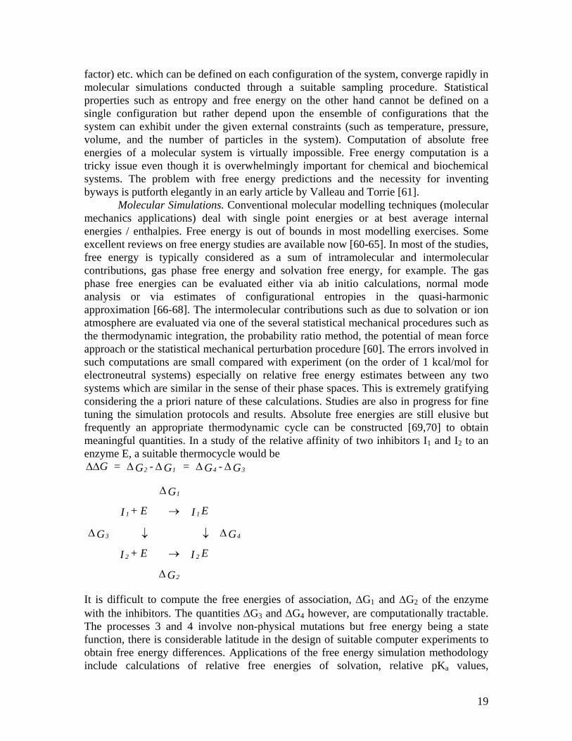
factor) etc. which can be defined on each configuration of the system, converge rapidly in molecular simulations conducted through a suitable sampling procedure. Statistical properties such as entropy and free energy on the other hand cannot be defined on a single configuration but rather depend upon the ensemble of configurations that the system can exhibit under the given external constraints (such as temperature, pressure, volume, and the number of particles in the system). Computation of absolute free energies of a molecular system is virtually impossible. Free energy computation is a tricky issue even though it is overwhelmingly important for chemical and biochemical systems. The problem with free energy predictions and the necessity for inventing byways is putforth elegantly in an early article by Valleau and Torrie [61]. Molecular Simulations. Conventional molecular modelling techniques (molecular mechanics applications) deal with single point energies or at best average internal energies / enthalpies. Free energy is out of bounds in most modelling exercises. Some excellent reviews on free energy studies are available now [60-65]. In most of the studies, free energy is typically considered as a sum of intramolecular and intermolecular contributions, gas phase free energy and solvation free energy, for example. The gas phase free energies can be evaluated either via ab initio calculations, normal mode analysis or via estimates of configurational entropies in the quasi-harmonic approximation [66-68]. The intermolecular contributions such as due to solvation or ion atmosphere are evaluated via one of the several statistical mechanical procedures such as the thermodynamic integration, the probability ratio method, the potential of mean force approach or the statistical mechanical perturbation procedure [60]. The errors involved in such computations are small compared with experiment (on the order of 1 kcal/mol for electroneutral systems) especially on relative free energy estimates between any two systems which are similar in the sense of their phase spaces. This is extremely gratifying considering the a priori nature of these calculations. Studies are also in progress for fine tuning the simulation protocols and results. Absolute free energies are still elusive but frequently an appropriate thermodynamic cycle can be constructed [69,70] to obtain meaningful quantities. In a study of the relative affinity of two inhibitors I1 and I2 to an enzyme E, a suitable thermocycle would be ∆∆ ∆ ∆ ∆ ∆G = G - G = G - G2 1 4 3

G

I + E I E

G G

I + E I E

G

1

1 1

3 4

2 2

2

∆

∆ ∆

∆

→

↓ ↓

→

It is difficult to compute the free energies of association, ∆G1 and ∆G2 of the enzyme with the inhibitors. The quantities ∆G3 and ∆G4 however, are computationally tractable. The processes 3 and 4 involve non-physical mutations but free energy being a state function, there is considerable latitude in the design of suitable computer experiments to obtain free energy differences. Applications of the free energy simulation methodology include calculations of relative free energies of solvation, relative pKa values,

19

conformational preferences in solution etc.. Extensions to binding and molecular recognition have also been forthcoming. Merits and limitations of a decomposition of free energy in terms of specific interactions have recently been analyzed carefully by Karplus [81], van Gunsteren [82] and their coworkers. Molecular simulations and free energy techniques may be essentially seen as a culmination of the pioneering efforts of Gibbs, Kirkwood, Zwanzig and others. Statistical mechanics has come to fruition in its applications to chemistry and biochemistry. The nature of the problems that confront the practitioners are very different now. To widen the scope of applicability of statistical mechanics, to understand structure and thermodynamics at a molecular level, one needs computationally efficient and accurate methods which can be routinely used by theoreticians or experimentalists on systems of interest. A severe limitation of the simulation techniques is that these are computationally expensive. A regular Metropolis Monte Carlo or a molecular dynamics simulation (seeking structural, dynamic and internal energy information) on a 216 particle liquid water system or a single ion in 215 waters takes about one hour on a Cray Y-MP. A simulation of protein-DNA complex with sufficient waters to provide two layers around the complex takes about 500 hours on Cray Y-MP. The same systems require ten times more CPU when a free energy related quantity is sought. In short, a single free energy determination can take any where from 10 to 1000 CPU hours on a supercomputer depending upon the level of detail and complexity of the problem which puts the free energy predictions starting from a molecular description of the system, beyond the reach of bench chemists and most theoreticians around the globe, without access to supercomputers. Ways have to be found to cut down on the computational time. If molecular modeling has to have its desired impact on chemical and pharmaceutical industry, development of suitable methodologies for an expeditious evaluation of free energies of molecular systems is essential. Dielectric Continuum methods. Free energy on the other hand is accessible with relative ease via the dielectric continuum approaches, analytical or numerical. Analytical methods have a long history [83]. Born model for ion solvation and Onsager's reaction field approach to dipolar solvation found a generalization in Kirkwood's formulation of the Helmholtz free energy of an arbitrary charge distribution embedded in a dielectric continuum solvent with added salt [84]. Beveridge and Schnuelle [85] reported a concentric dielectric model which can in principle incorporate several layers of solvent with varying "dielectric constants" to account for saturation effects in calculating solvation free energies of arbitrary charge distributions with an overall spherical symmetry. This theory was subsequently extended to other geometries [86-88]. Extensions to Tanford-Kirkwood theory [89] were also reported [90] and results compared with those based on molecular simulations [91]. Solvation and salt effects in the stability of globular proteins, for instance, fall within the purview of such theories. The SATK (static accessibility Tanford-Kirkwood) model [92], which uses a simpler treatment of solvent than that of Beveridge and coworkers but an additional depth parameter has been extensively applied to study protein titration curves, merits and limitations of which are discussed in several places [92,93]. States and Karplus [94] developed an electrostatic continuum solvent model to treat hydrogen exchange behavior in proteins [95]. Molecular simulations have provided new insights into the success of continuum models and have repeatedly validated the underlying approximations in the

20

continuum models [96-99]. The above theories deal with solvent and / or salt effects on an ion, a molecule or a macromolecule. Dielectric continuum theories for binding and interaction have progressed beyond the Coulomb's law only recently [100]. On the numerical front, there is a constant methodological influx for calculating electrostatic contribution to free energies of biomolecular systems. The protein dipole Langevin dipole (PDLD) approach [101], the finite boundary element method [102], the finite difference Poisson-Boltzmann (FDPB) method [103-112] and the finite element method [113] are some of the techniques to capture the electrostatics of a given system, the FDPB method being the most widely used (Delphi package distributed by BIOSYM Technologies / MSI) for quantitative predictions [114-126]. All these are based on solutions (analytical / numerical) to the nonlinear Poisson-Boltzmann equation:

∇ ∇Φ[D(r) (r)] - [ (r)] + 4 (r) = 02 fκ π ρsinh Φ

Φ in the above equation is the electrostatic potential, D(r) is the dielectric function, is a modified Debye-Huckel parameter and ρf is the fixed charge distribution of the molecular system.The electrostatic potential obtained by solving the above equation is then used to calculate the free energies as a sum over the product of charges and potentials or as a volume integral of the product of electric field and dielectric displacement. The generalized Born models in vogue today [Still, 1990, Cramer & Truhlar, 1994, 1996a 1996b]] present an even simpler treatment of solvent than the FDPB method and are designed to capture the electrostatics of solvation in a computationally efficient manner. In such studies, only the electrostatic component can be calculated. The results have to be supplemented with non-electrostatic contributions to free energy. Continuum methods deserve special attention for free energy estimates in view of the rapidity with which these calculations can be performed. The results however, are sensitive to the choice of parameters such as cavity or van der Waals radii, partial atomic charges etc.. These parameters have to be tested against molecular simulations or experiment and particularly the consequences of neglecting molecular solvent have to be closely examined. Force field comparisons with continuum model solvent have been undertaken recently [127,128] Some recent reviews [129-137] have summarized the existing theoretical tools to treat electrostatic effects in biological molecules. A recent article by Honig and Nicholls [138] sums up the current status on the applications of classical electrostatics to biomolecules. Empirical Approaches. Other class of methods for estimating free energies comprise empirical techniques for probing solvation effects based on hydration shell volumes [68,139-142] and accessible surface areas [143-145]. These hinge upon the idea that solvation free energies could be estimated with a PV or γA type term where P and V, γ and A denote pressure, volume, surface tension and area respectively. In the excluded volume approach [141,142], hydration shell volumes excluded due to the encroachment of hydration spheres of any two atoms in a given conformation are calculated analytically or numerically. These excluded volumes are then multiplied by an appropriate free energy density parameter to obtain solvation free energies of a given molecular system in a specified conformation. In the accessible area approach [146-151], solvent accessibility (area) of each atom in the molecule is computed and multiplied by an atomic solvation

21

parameter to obtain solvation free energies. This is a particularly useful technique to estimate the hydrophobic contribution to the total free energy of the system. In all these cases, a careful calibration of the parameters involved (free energy densities / atomic solvation parameters etc.) for a given class of compounds is required to obtain quantitatively correct results. 4. Rate Constants 4.1 Brownian Dynamics A number of bimolecular events are diffusion controlled. The rate constants for such reactions are on the order of 109M-1sec-1 [153]. Brownian dynamics simulations are a natural choice for monitoring macromolecular association in the nanosecond to microsecond regime and for determining the rate constants. Also, Brownian dynamics is appropriate for describing macromolecular motions over distances which are large compared to the solvent size and times that are long compared to the interval between successive solvent impacts. Brownian dynamics simulations are carried out typically by integrating the Langevin equation of motion. m r r F fi i ij

jj i ij

jj&& &= − + +∑ ∑ς α

Here mi is the mass of the ith particle, ri is its position, ri its velocity, ζij is the configuration dependent friction tensor, and Fi is the force on the ith particle due to other particles and any external force. αijfj is a randomly fluctuating force on the particle due to the surrounding solvent, where fj obeys a gaussian distribution. The displacement equation for the spatial evolution of the solute in a continuum solvent over a time interval ∆t is given as

r rt

k TD t F t

D tr

t R tB

ij jj

ij

ji' ( ) ( )

( )( )= + + +∑ ∑∆

∆ ∆∂

∂

where r and r’ are the initial and final position vectors, kBT is the product of the Boltzmann constant and temperature, F is the systematic intermolecular force and D the hydrodynamic tensor. R represents the stochastic displacement and is a vector of Gaussian random numbers with the properties <Ri>=0 and <RiRj>=2Dij∆t. The random displacement R is calculated by generating normal random deviates [xi : <xi>=0, <xixj>=2δijD∆t] Some of the choices for a diffusion tensor as an approximation to the hydrodynamic interactions are the Oseen tensor, or a constant diffusion tensor. The modified Oseen tensor with stick conditions is given as

Dk T

rI

r rr r

I r rrij

B

ij

ij ij

ij

i j

ij

ij ij

ij= + +

+−

⎛

⎝⎜

⎞

⎠⎟

⎡

⎣⎢

⎤

⎦⎥

8 32

2 2

2 2πησ σ

For the case with no hydrodynamic interactions, the tensor is replaced by a diffusion constant representing the motion of the solute molecule.

22

Dk T

aB=

6πη

where a is the hydrodynamic radius and η is the coefficient of viscosity of the solvent. The justification for using a simple diffusion model in many Brownian dynamics problems comes from the observation that rate processes are often weakly affected by changes in the hydrodynamic approximation although this is not always the case for asymmetric solutes. All these tensors have the property

∂∂

D trij

jj

( )∑ = 0

In a simulation of a ligand executing Brownian motion relative to a receptor and reaching the actve site, the rate constant k can be computed from the encounter probabilities as

kk bD=

− −( )

( )β

β1 1 Ω

where b is the probability that the ligand initially at b reaches the active site rather than escapes, Ω =kD(b)/kD(q) where q is the truncation radius. If b is chosen large enough that forces are centrosymmetric for distances larger than b

k be

r D rdrD

U r k T

b

B

( )( )

( )/

=⎡

⎣⎢

⎤

⎦⎥

∞ −

∫ 4 2

1

π

where U(r) is the potential of mean force and D(r) the relative diffusion tensor. In the special case where U(r)=0 for r>b and no hydrodynamic interaction, the Smoluchowski result is obtained. kD(b)=4πDb. Kinetic studies are out of bounds in most cases except for diffusion controlled reactions where some structural data is available on the complex. The time scales for the kinetic investigations are mostly out of reach of the present day computer capacity. Simulations at this stage, can provide some useful information at a molecular level, on diffusion controlled reactions.

23