Theoretical methods for the electronic structure …1050660/FULLTEXT01.pdfthe electronic structure...

ACTAUNIVERSITATIS

UPSALIENSISUPPSALA

2017

Digital Comprehensive Summaries of Uppsala Dissertationsfrom the Faculty of Science and Technology 1461

Theoretical methods forthe electronic structure andmagnetism of strongly correlatedmaterials

INKA L. M. LOCHT

ISSN 1651-6214ISBN 978-91-554-9770-5urn:nbn:se:uu:diva-308699

Dissertation presented at Uppsala University to be publicly examined in Ång/10132,Häggsalen, Ångströmlaboratoriet, Lägerhyddsvägen 1, Uppsala, Friday, 3 February 2017 at09:15 for the degree of Doctor of Philosophy. The examination will be conducted in English.Faculty examiner: Prof. Dr. Silke Biermann (CPHT, Ecole Polytechnique).

AbstractLocht, I. L. M. 2017. Theoretical methods for the electronic structure and magnetism ofstrongly correlated materials. Digital Comprehensive Summaries of Uppsala Dissertationsfrom the Faculty of Science and Technology 1461. 109 pp. Uppsala: Acta UniversitatisUpsaliensis. ISBN 978-91-554-9770-5.

In this work we study the interesting physics of the rare earths, and the microscopic stateafter ultrafast magnetization dynamics in iron. Moreover, this work covers the development,examination and application of several methods used in solid state physics. The first and thelast part are related to strongly correlated electrons. The second part is related to the field ofultrafast magnetization dynamics.

In the first part we apply density functional theory plus dynamical mean field theory withinthe Hubbard I approximation to describe the interesting physics of the rare-earth metals. Theseelements are characterized by the localized nature of the 4f electrons and the itinerant characterof the other valence electrons. We calculate a wide range of properties of the rare-earth metalsand find a good correspondence with experimental data. We argue that this theory can be thebasis of future investigations addressing rare-earth based materials in general.

In the second part of this thesis we develop a model, based on statistical arguments, topredict the microscopic state after ultrafast magnetization dynamics in iron. We predict that themicroscopic state after ultrafast demagnetization is qualitatively different from the state afterultrafast increase of magnetization. This prediction is supported by previously published spectraobtained in magneto-optical experiments. Our model makes it possible to compare the measureddata to results that are calculated from microscopic properties. We also investigate the relationbetween the magnetic asymmetry and the magnetization.

In the last part of this work we examine several methods of analytic continuation that are usedin many-body physics to obtain physical quantities on real energies from either imaginary timeor Matsubara frequency data. In particular, we improve the Padé approximant method of analyticcontinuation. We compare the reliability and performance of this and other methods for bothone and two-particle Green's functions. We also investigate the advantages of implementinga method of analytic continuation based on stochastic sampling on a graphics processing unit(GPU).

Keywords: dynamical mean field theory (DMFT), Hubbard I approximation, stronglycorrelated systems, rare earths, lanthanides, photoemission spectra, ultrafast magnetizationdynamics, analytic continuation, Padé approximant method, two-particle Green's functions,linear muffin tin orbitals (LMTO), density functional theory (DFT), cerium, stacking faultenergy.

Inka L. M. Locht, Department of Physics and Astronomy, Materials Theory, Box 516, UppsalaUniversity, SE-751 20 Uppsala, Sweden.

© Inka L. M. Locht 2017

ISSN 1651-6214ISBN 978-91-554-9770-5urn:nbn:se:uu:diva-308699 (http://urn.kb.se/resolve?urn=urn:nbn:se:uu:diva-308699)

List of papers

This thesis is based on the following papers, which are referred to in the text

by their Roman numerals.

I Standard model of the rare-earths, analyzed from the Hubbard Iapproximation.I. L. M. Locht, Y. O. Kvashnin, D. C. M. Rodrigues, M. Pereiro, A.

Bergman, L. Bergqvist, A. I. Lichtenstein, M. I. Katsnelson, A. Delin,

A. B. Klautau, B. Johansson, I. Di Marco and O. Eriksson,

PHYSICAL REVIEW B 94, 085137 (2016)

II Stacking fault energetics of α- and γ-cerium investigated with abinitio calculations.A. Östlin, I. Di Marco, I. L. M. Locht, J. C. Lashley and L. Vitos,


III Ultrafast magnetization dynamics: Microscopic electronicconfigurations and ultrafast spectroscopy.I. L. M. Locht, I. Di Marco, S. Garnerone, A. Delin and M. Battiato,


IV Draft of: Magnetic asymmetry around the 3p absorption edge inFe and NiI. L. M. Locht, S. Jana, Y. O. Kvashnin, R. Knut, I. Di Marco, R.

Chimata, R. S. Malik, M. Ahlberg, M. Battiato, J. Rusz, R. Stefanuik,

J. Söderström, T. J. Silva, J. Åkerman, H. T. Nembach, J. M. Shaw, O.

Karis, O. Eriksson,

In preparation

V Analytic continuation by averaging Padé approximants.J. Schött, I. L. M. Locht, E. Lundin, O. Grånäs, O. Eriksson and I. Di

Marco,


VI A comparison between methods of analytical continuation forbosonic functions.J. Schött, E. G. C. P. van Loon, I. L. M. Locht, M. I. Katsnelson and I.

Di Marco,

accepted in PRB

VII A GPU code for analytic continuation through a sampling method.J. Nordström, J. Schött, I. L. M. Locht, and I. Di Marco, accepted in

SoftwareX

Reprints were made with permission from the publishers.

Publications not included in this thesis:

Reproducibility in density functional theory calculations of solids.K. Lejaeghere et al., Science 351, 6280 (2016)

Comments on my participationThe main project during my PhD was to apply the Hubbard I approximation

to describe the electronic structure of the rare earths. I did all calculations on

the cohesive properties, structural stabilities, ground-state magnetic moments

and the valence-band spectra. The exchange parameters were calculated by

Yaroslav Kvashnin and the resulting ordering temperatures and magnon spec-

tra were calculated by Debora Rodrigues and Manuel Pereiro. I analyzed most

data and contributed to obtain a consistent physical picture. The research was

planned by Igor Di Marco and Olle Eriksson and also by myself in a later

stage. Paper I is mainly written by me. For Paper II, I performed all Hubbard

I calculations, and participated in discussions.

The development of the model presented in Paper III to predict the micro-

scopic state directly after ultrafast magnetization dynamics was a joint effort

by me, Igor Di Marco and Marco Battiato, with help of Silvano Garnerone and

Anna Delin. For both Paper III and IV I participated in planning the research,

developing the theory, discussing the results and writing the paper. All DFT

calculations in Papers III and IV are done by me.

The improvement of the Padé approximant method was mainly planned by

Igor Di Marco and Johan Schött, who developed the routines and performed

the calculations. Elin Lundin and I started this work as part of her bachelor

student project. When Johan Schött joined the group he took over the project.

I participated in analyzing the results, planning the next steps and also in writ-

ing the paper. For Paper VI, I initiated the collaboration with and Erik van

Loon and Mikhail Katsnelson. I participated in planning the research, dis-

cussing, analyzing the results, and writing the article. The calculations were

done by Johan Schött. The GPU implementation for the analytic continuation

was done by Johan Nordström as part of an independent bachelor work for

technical physics. I got involved in this as project mentor of Johan Nordström.

I participated in analyzing the results, writing the paper and preparing the code

for publication.

Finally, in all works, I contributed to discuss the criticism raised by the

referees and to write appropriate replies.

Contents

1 Introduction . . . . . . . . . . . . . . . . . . . . . . . . . . . . . . . . . . . . . . . . . . . . . . . . . . . . . . . . . . . . . . . . . . . . . . . . . . . . . . . . . . . . . . . . . . . . . . . . . . 7

2 Methods . . . . . . . . . . . . . . . . . . . . . . . . . . . . . . . . . . . . . . . . . . . . . . . . . . . . . . . . . . . . . . . . . . . . . . . . . . . . . . . . . . . . . . . . . . . . . . . . . . . . . . 10

2.1 Solid state Hamiltonian . . . . . . . . . . . . . . . . . . . . . . . . . . . . . . . . . . . . . . . . . . . . . . . . . . . . . . . . . . . . . . . . . . 11

2.2 Density Functional Theory . . . . . . . . . . . . . . . . . . . . . . . . . . . . . . . . . . . . . . . . . . . . . . . . . . . . . . . . . . . . 12

2.2.1 Hohenberg-Kohn theorems . . . . . . . . . . . . . . . . . . . . . . . . . . . . . . . . . . . . . . . . . . . . . 12

2.2.2 Kohn-Sham ansatz . . . . . . . . . . . . . . . . . . . . . . . . . . . . . . . . . . . . . . . . . . . . . . . . . . . . . . . . . . . 13

2.2.3 Approximations to the energy functional . . . . . . . . . . . . . . . . . . . . . . . 16

2.2.4 LMTO and LAPW bases . . . . . . . . . . . . . . . . . . . . . . . . . . . . . . . . . . . . . . . . . . . . . . . . . 17

2.3 Hubbard I approximation . . . . . . . . . . . . . . . . . . . . . . . . . . . . . . . . . . . . . . . . . . . . . . . . . . . . . . . . . . . . . . . 19

2.3.1 Effective Hubbard model . . . . . . . . . . . . . . . . . . . . . . . . . . . . . . . . . . . . . . . . . . . . . . . . 21

2.3.2 Effective Single impurity Anderson model . . . . . . . . . . . . . . . . . . 22

2.3.3 Computational scheme . . . . . . . . . . . . . . . . . . . . . . . . . . . . . . . . . . . . . . . . . . . . . . . . . . . 26

2.3.4 Hubbard U and Hund’s J . . . . . . . . . . . . . . . . . . . . . . . . . . . . . . . . . . . . . . . . . . . . . . . 28

2.3.5 Double counting . . . . . . . . . . . . . . . . . . . . . . . . . . . . . . . . . . . . . . . . . . . . . . . . . . . . . . . . . . . . . . 31

3 Lanthanides . . . . . . . . . . . . . . . . . . . . . . . . . . . . . . . . . . . . . . . . . . . . . . . . . . . . . . . . . . . . . . . . . . . . . . . . . . . . . . . . . . . . . . . . . . . . . . . . 33

3.1 Outer electronic configuration . . . . . . . . . . . . . . . . . . . . . . . . . . . . . . . . . . . . . . . . . . . . . . . . . . . . . . . 34

3.2 Bonding properties . . . . . . . . . . . . . . . . . . . . . . . . . . . . . . . . . . . . . . . . . . . . . . . . . . . . . . . . . . . . . . . . . . . . . . . . . 34

3.3 Structural stabilities . . . . . . . . . . . . . . . . . . . . . . . . . . . . . . . . . . . . . . . . . . . . . . . . . . . . . . . . . . . . . . . . . . . . . . . 36

3.4 Magnetism . . . . . . . . . . . . . . . . . . . . . . . . . . . . . . . . . . . . . . . . . . . . . . . . . . . . . . . . . . . . . . . . . . . . . . . . . . . . . . . . . . . . . . 37

3.4.1 Coupling of spin and orbital moments . . . . . . . . . . . . . . . . . . . . . . . . . . . 37

3.4.2 Moments arising from the spin, orbital and total

angular momenta . . . . . . . . . . . . . . . . . . . . . . . . . . . . . . . . . . . . . . . . . . . . . . . . . . . . . . . . . . . . . 38

3.4.3 Magnetic moments in a magnetic field . . . . . . . . . . . . . . . . . . . . . . . . . . 40

3.5 Spectral properties . . . . . . . . . . . . . . . . . . . . . . . . . . . . . . . . . . . . . . . . . . . . . . . . . . . . . . . . . . . . . . . . . . . . . . . . . . 43

3.5.1 Spectroscopy . . . . . . . . . . . . . . . . . . . . . . . . . . . . . . . . . . . . . . . . . . . . . . . . . . . . . . . . . . . . . . . . . . . . 43

3.5.2 Experiment and theory . . . . . . . . . . . . . . . . . . . . . . . . . . . . . . . . . . . . . . . . . . . . . . . . . . . . 44

3.5.3 Multiplet structure . . . . . . . . . . . . . . . . . . . . . . . . . . . . . . . . . . . . . . . . . . . . . . . . . . . . . . . . . . . 46

3.6 Summary of Papers I and II . . . . . . . . . . . . . . . . . . . . . . . . . . . . . . . . . . . . . . . . . . . . . . . . . . . . . . . . . . . 46

3.7 Outlook . . . . . . . . . . . . . . . . . . . . . . . . . . . . . . . . . . . . . . . . . . . . . . . . . . . . . . . . . . . . . . . . . . . . . . . . . . . . . . . . . . . . . . . . . . . 49

4 Microscopic configuration after ultrafast magnetization dynamics . . . . . . . 51

4.1 Summary of Paper III: Microscopic configuration after ultrafast

magnetization dynamics . . . . . . . . . . . . . . . . . . . . . . . . . . . . . . . . . . . . . . . . . . . . . . . . . . . . . . . . . . . . . . . . 53

4.2 Magneto-optics . . . . . . . . . . . . . . . . . . . . . . . . . . . . . . . . . . . . . . . . . . . . . . . . . . . . . . . . . . . . . . . . . . . . . . . . . . . . . . . 56

4.2.1 Experiments . . . . . . . . . . . . . . . . . . . . . . . . . . . . . . . . . . . . . . . . . . . . . . . . . . . . . . . . . . . . . . . . . . . . . 57

4.2.2 Dielectric tensor . . . . . . . . . . . . . . . . . . . . . . . . . . . . . . . . . . . . . . . . . . . . . . . . . . . . . . . . . . . . . . . 58

4.2.3 Relation asymmetry and dielectric tensor . . . . . . . . . . . . . . . . . . . . . . 59

4.3 Is the magnetic asymmetry proportional to the sample

magnetization? . . . . . . . . . . . . . . . . . . . . . . . . . . . . . . . . . . . . . . . . . . . . . . . . . . . . . . . . . . . . . . . . . . . . . . . . . . . . . . . 60

4.3.1 Before the laser pulse: equilibrium situation . . . . . . . . . . . . . . . . . 60

4.3.2 After the laser pulse: recovering the equilibrium

magnetization . . . . . . . . . . . . . . . . . . . . . . . . . . . . . . . . . . . . . . . . . . . . . . . . . . . . . . . . . . . . . . . . . . . 62

4.4 Outlook . . . . . . . . . . . . . . . . . . . . . . . . . . . . . . . . . . . . . . . . . . . . . . . . . . . . . . . . . . . . . . . . . . . . . . . . . . . . . . . . . . . . . . . . . . . 66

5 Analytic continuation . . . . . . . . . . . . . . . . . . . . . . . . . . . . . . . . . . . . . . . . . . . . . . . . . . . . . . . . . . . . . . . . . . . . . . . . . . . . . . . . 68

5.1 Spectral functions . . . . . . . . . . . . . . . . . . . . . . . . . . . . . . . . . . . . . . . . . . . . . . . . . . . . . . . . . . . . . . . . . . . . . . . . . . . 68

5.2 Methods of analytic continuation . . . . . . . . . . . . . . . . . . . . . . . . . . . . . . . . . . . . . . . . . . . . . . . . . . 70

5.2.1 Padé approximant method . . . . . . . . . . . . . . . . . . . . . . . . . . . . . . . . . . . . . . . . . . . . . . . 72

5.2.2 Stochastic Sampling . . . . . . . . . . . . . . . . . . . . . . . . . . . . . . . . . . . . . . . . . . . . . . . . . . . . . . . 76

5.2.3 Least square solutions and regularizations . . . . . . . . . . . . . . . . . . . 78

5.3 Remarks on performance . . . . . . . . . . . . . . . . . . . . . . . . . . . . . . . . . . . . . . . . . . . . . . . . . . . . . . . . . . . . . . . 82

5.4 Summary of Papers V, VI and VII . . . . . . . . . . . . . . . . . . . . . . . . . . . . . . . . . . . . . . . . . . . . . . . . 82

5.5 Outlook . . . . . . . . . . . . . . . . . . . . . . . . . . . . . . . . . . . . . . . . . . . . . . . . . . . . . . . . . . . . . . . . . . . . . . . . . . . . . . . . . . . . . . . . . . . 86

Popular scientific summary . . . . . . . . . . . . . . . . . . . . . . . . . . . . . . . . . . . . . . . . . . . . . . . . . . . . . . . . . . . . . . . . . . . . . . . . . . . . . 88

Populärvetenskaplig sammanfattning . . . . . . . . . . . . . . . . . . . . . . . . . . . . . . . . . . . . . . . . . . . . . . . . . . . . . . . . . . . . . 91

Populair wetenschappelijke samenvatting . . . . . . . . . . . . . . . . . . . . . . . . . . . . . . . . . . . . . . . . . . . . . . . . . . . . . . 94

Acknowledgements . . . . . . . . . . . . . . . . . . . . . . . . . . . . . . . . . . . . . . . . . . . . . . . . . . . . . . . . . . . . . . . . . . . . . . . . . . . . . . . . . . . . . . . . . . 97

Appendices . . . . . . . . . . . . . . . . . . . . . . . . . . . . . . . . . . . . . . . . . . . . . . . . . . . . . . . . . . . . . . . . . . . . . . . . . . . . . . . . . . . . . . . . . . . . . . . . . . . . . . . 99

A Finding the multiplets in Nd . . . . . . . . . . . . . . . . . . . . . . . . . . . . . . . . . . . . . . . . . . . . . . . . . . . . . . . . . . . . . . . . . . . 100

References . . . . . . . . . . . . . . . . . . . . . . . . . . . . . . . . . . . . . . . . . . . . . . . . . . . . . . . . . . . . . . . . . . . . . . . . . . . . . . . . . . . . . . . . . . . . . . . . . . . . . . 103

1. Introduction

ABOUT one year ago, my cousin asked me: “What do you actually

do?” An innocent question of a kid. I faced myself the challenge

of explaining to a 9 year old about computational material theory,

about the ins and outs of the Hubbard I approximation and about

the concept of analytic continuation. The discussion following this question

involved lego bricks representing the different atoms in the periodic table and

how one can build, with only “carbon lego bricks”, shiny diamonds as well

as the soft black graphite stick in your pencil. It involved dancing couples

representing the spin up and spin down pairs in the same orbital and how one

could predict their behavior and their influence on the other dancers. In this

thesis I aim to explain my work on a more fundamental level. I wish you great

fun reading it and I hope you will enjoy it as much as I did doing the research

which underlies this thesis.

Materials have always been important for mankind. Also nowadays the de-

velopment of many applications is restricted by the properties, the scarcity and

the costs of the materials involved. Imagine a feature-full smartphone with a

battery that needs to be charged only once a month, although you use its full

capabilities. Imagine a panel of highly efficient, payable solar-cells on your

roof. Or imagine much faster and more energy efficient data storage and sens-

ing devises. These are only a few examples for which we need new materials

with more and more desired properties. To find these materials the joint effort

of experimentalists, theoreticians and engineers in the field of material science

is required. My modest contribution to the field is of theoretical nature. I think

that the theoretical research in material science can be decomposed in two cat-

egories. On the one hand, the more applied category, in which the research

focusses on the direct search for materials with a set of desired properties.

On the other hand, the more fundamental category of model and method de-

velopment. My thesis falls in the second category: we examine a method to

describe the electronic structure of the rare earths, we improve and extensively

test different methods of analytic continuation, and we also develop a model

to predict the microscopic state after ultrafast magnetization dynamics. With

this we hope to contribute to the improvement of the state-of-the-art methods

used in material science.

After this introduction, Chapter 2 is a method chapter, that briefly intro-

duces density functional theory and its combination with dynamical mean field

theory. The remaining of the thesis is divided in three themed chapters.

7

Chapter 3: The first theme comprises the rare-earth elements. These atoms

are found in a wide range of functional materials and it is very important

to have a practical theoretical tool to describe them. Several attempts have

been made to determine the electronic structure of the rare earths with ab ini-tio methods. These elements are characterized by the localized nature of the

4 f electrons and the itinerant character of the other valence electrons. Since

density functional theory with the common parametrizations of the exchange-

correlation functional cannot capture the correlated f electrons, more sophisti-

cated theories have been tried [4, 81, 30, 88]. Although some of these methods

turned out to be very accurate for selected properties, none of them can give a

unified picture of the physics of the rare earths. In Paper I we intend to do pre-

cisely this. We propose density functional theory plus dynamical mean field

theory within the Hubbard I approximation to describe the interesting physics

of the rare-earth metals and rare earth containing materials. In Chapter 3 we

introduce the reader to several defining properties of the rare earths and we try

to make insightful why the Hubbard I approximation is expected to perform

well. In Paper I we examine a wide range of properties of the rare-earth metals

and we argue that our theory can be a firm basis for the future investigation

of generic rare-earth based materials. In Paper II we use the excellent perfor-

mance of the Hubbard I approximation to calculate the stacking fault energies

in γ-Cerium.

Chapter 4: The second theme is related to the field of ultrafast magnetiza-

tion dynamics. The possibility of manipulating the magnetization within a few

hundreds of femtoseconds [12] has induced great excitement in the scientific

community. This field is characterized by femtosecond dynamics resulting in

corresponding strongly-out-of-equilibrium physics. Needless to say, this out-

of-equilibrium physics is very complicated to address theoretically. In Chap-

ter 4 and Paper III we intend to connect theory to experiments performed in the

field of ultrafast magnetization dynamics. Or, in other words, we want to con-

nect the microscopic physics of the system to the properties that are probed in

the experiments. We propose a model that is based on statistical arguments for

a system in a partial thermal equilibrium. We identify the microscopic config-

uration of the system directly after the ultrafast magnetization dynamics have

finished. This model makes it possible to connect theoretical calculations orig-

inating at the microscopic level to averages of macroscopic quantities. With

our predictions we can calculate the dielectric response around the 3p absorp-

tion edge of Fe at the end of the ultrafast magnetization dynamics, but before

the full equilibrium is recovered. This dielectric response is compared to the

experimentally measured T-MOKE asymmetry [86, 93].

Chapter 5: The third theme has a more methodological nature. Strongly

correlated materials are currently of great interest and exhibit many exotic ef-

fects which may be important for technological applications. However, it is

very difficult to determine their electronic structure. The increase of compu-

tational power has lead to several computational methods, such as dynamical

8

mean field theory or the GW approach. Most implementations of these meth-

ods, perform parts of the calculations in the imaginary-time or imaginary-

frequency domain for technical reasons. Since real physical quantities depend

on real time or real energies instead, a reliable tool is required to obtain those

quantities from the functions in the imaginary-time or imaginary-frequency

domain. These tools are commonly referred to as methods of analytic con-

tinuation. In Chapter 5 we briefly introduce several methods of analytic con-

tinuations. Paper V, VI and VII are closely connected to this chapter. In

Paper V we propose a remedy to the well-known problems of the Padé approx-

imant method by performing an average of several continuations, obtained by

varying the number of fitted input points and Padé coefficients independently.

We subject this method to extensive performance and reliability tests for one-

particle Green’s functions. In Paper VI we focus on dynamical two-paricle

quantities, instead, and evaluate the strengths and weaknesses of several dif-

ferent methods of analytic continuation. In Paper VII we switch our attention

to computational performance. We investigate the advantages of implement-

ing a method of analytic continuation based on stochastic sampling [70] on a

graphics processing unit (GPU). This implementation allows to save compu-

tational time on supercomputer clusters by allowing extensive calculations to

be performed on a common laptop.

Having outlined the structure of this thesis, I wish you an enjoyable reading

of it!

9

2. Methods

IN this chapter we will provide a background to the methods to calcu-

late the electronic structure of materials used in this thesis. In Sec. 2.1

we describe the general problem-to-solve in solid state physics and in

Sec. 2.2 we arrive at density functional theory (DFT) as one of the pos-

sible (approximate) ways to calculate the electronic structure.

Despite the approximations that have to be made to the exchange-correlation

functional, standard DFT works very well for a large class of materials. How-

ever, for some materials, strong correlations have to be taken into account.

One way to do this is to combine DFT with the dynamical mean field theory

(DMFT), which is explained in Sec. 2.3. The chapter closes with the Hubbard

I approximation (HIA), which is an approximation to DFT+DMFT.

This method chapter is related to the other chapters in quite different ways.

In Paper I we show that the DFT+DMFT(HIA) method is very suitable to

describe several properties of the REs. In Chapter 3 we introduce these prop-

erties and also try to make insightful why the HIA is advisable for this class

of elements. In Paper III and Chapter 4 we develop a model to predict the mi-

croscopic state directly after ultrafast magnetization dynamics. In this project,

DFT calculations are only a small part of a larger whole. Chapter 5 is actu-

ally a method chapter, dedicated to a special problem encountered in DMFT,

i.e. the analytic continuation. In most DMFT implementations, quantities are

calculated as a function of imaginary time or imaginary frequency. However,

real world quantities are measured as a function of real time or real frequency.

To compare theory and experiment, one has to obtain these quantities from the

calculated ones. In Paper V, VI and VII, we investigate several methods how

to do this. In this sense, Chapter 5, in which these papers are prefaced, is an

other method chapter, specifically tailored to methods of analytical continua-

tion.

In the current chapter we only briefly mention technicalities related to our

implementation of DFT+DMFT. In Sec. 2.2.4 we outline the difference be-

tween the basis sets employed by the codes used in Paper I, II and III. How-

ever, we refer the interested reader to these papers or to Ref. [62] for more

precise details on the basis. The latter is my licentiate thesis, where I explain

the code and the basis used in Paper I, and the corresponding choices and op-

timizations of the basis for the lanthanides. This method chapter is largely

based on Chapter 3 of my licentiate thesis [62].

10

2.1 Solid state Hamiltonian

A collection of atoms consists of nuclei and electrons which all interact. This

results in a Hamiltonian with 5 different terms. Two kinetic terms, one for

the electrons and one for the nuclei and three Coulomb terms. The latter de-

scribe the attraction between the positively charged nuclei and the negatively

charged electrons and the repulsion between electrons and nuclei themselves.

For simplicity we will ignore the relativistic effects, but the Schrödinger equa-

tion can be generalized to the Dirac equation. The above described Hamilto-

nian looks quite simple. However, already for a few atoms, the computational

effort needed for a full quantum mechanical solution runs out of control and

we are left with an unsolvable Hamiltonian. The first simplifying approxima-

tion is given by the Born-Oppenheimer approximation [16] which separates

the electronic and ionic degrees of freedom. Given that the kinetic term is in-

versely proportional to the mass, the kinetic term of the nuclei is much smaller

than the kinetic term of the electrons. To describe the electronic degrees of

freedom, the positions of the nuclei can be approximated as fixed, constituting

a static external potential for the electrons. The Hamiltonian for the electronic

degrees of freedom reduces then to

H =−h2

2me∑

i∇2

i +∑i

Vext(ri)+1

2∑i�= j

e2

|ri− r j| , (2.1)

where the indices i and j run over the different electrons. The kinetic energy

of the electrons is given in the first term, where h is the Planck constant, methe electron mass and −ih∇ the momentum operator. The external potential

due to the ions is given in the second term and the last term is the Coulomb re-

pulsion between the electrons. Although this Hamiltonian can be diagonalized

for a few electrons, it quickly becomes impossible to do so when approach-

ing macroscopic solids. However, that is precisely what one would like to do,

since the eigenvalues of this Hamiltonian give the energy of the system and

the eigenfunctions give the electron many-body wave functions.

Before discussing how to tackle this problem, let us present the second

simplification one can make. This is based on the translational invariance of

a crystal. For translational invariant systems, the Bloch theorem [15] states

that the (one-electron) wave function ψ can be written as a periodic function

u(r), with the same periodicity as the crystal lattice under consideration, times

a plane wave:

ψk(r) = uk(r)eik·r, (2.2)

where k is the reciprocal lattice vector.

Although the Born-Oppenheimer approximation and the use of the Bloch

theorem greatly simplify the task of diagonalizing the Hamiltonian described

in the beginning of this section, a solution is still unreachable for more than

11

a few atoms and electrons. However, thanks to Pierre C. Hohenberg, Walter

Kohn, Lu Jeu Sham and many others, we nowadays have a very successful

way to tackle this problem: Density Functional Theory (DFT).

2.2 Density Functional Theory

The brilliant ideas that initiated the development of DFT were given by Pierre

C. Hohenberg, Walter Kohn and Lu Jeu Sham. Roughly speaking, Pierre C.

Hohenberg and Walter Kohn stated that if you have the ground-state density

of the particles in space and the interaction between the particles, you have, in

principle access to any property of the system. They formulated this statement

more precisely in two theorems known as the Hohenberg-Kohn theorems [45].

Later Walter Kohn and Lu Jeu Sham came with the Kohn-Sham ansatz [54]

that opened the route to modern DFT. The book Electronic Structure by Mar-

tin [64] is a very good reference, both for the fundamentals of DFT as well

as for practical electronic structure calculations. The current section is mainly

based on chapters 6 and 7 of this book.

2.2.1 Hohenberg-Kohn theorems

The Hohenberg-Kohn theorems lead to a simplification of the many-electron

problem by shifting the attention from the wave function, that depends on the

position vectors of all electrons simultaneously, to the density, that depends

on one position vector only. Precisely formulated, the Hohenberg-Kohn theo-

rems [64] read:

Theorem 1 For any system of interacting particles in an external potentialVext(r), the potential Vext(r) is determined uniquely, except for a constant, bythe ground-state particle density n0(r).

Corollary 1 Since the Hamiltonian is thus fully determined, except for a con-stant shift of the energy, it follows that the many-body wave functions for allstates (ground and excited) are determined. Therefore all properties of thesystem are completely determined given only the ground-state density n0(r).

Theorem 2 A universal functional of the energy E[n] in terms of the densityn(r) can be defined, valid for any external potential Vext(r). For any particularVext(r), the exact ground-state energy of the system is the global minimumvalue of this functional, and the density n(r) that minimizes the functional isthe exact ground-state density n0(r).

Corollary 2 The functional E[n] alone is sufficient to determine the exactground-state energy and density. In general, excited states of the electronsmust be determined by other means.

12

For the actually surprisingly simple proofs of these theorems I would like to

refer the reader to the nice explanation in chapter 6 of Electronic Structureby Martin [64]. In the scheme below, I summarize the first Hohenberg-Kohn

theorem, which will be related to the Kohn-Sham ansatz later in this text.

Vext(r)Hohenberg-Kohn

n0(r)

Ψ0({r})Ψi({r})H

With capital Ψi we denote the many-body wave functions and the subscript

zero denotes the ground state. Starting from the external potential Vext(r) and

going counter clock wise, one recognizes the scheme from quantum mechan-

ics. With the potential the Hamiltonian H can be constructed, that enters the

Schrödinger equation. Solving the Schrödinger equation gives the wave func-

tions Ψi(r), including the ground state Ψ0(r). From the ground-state wave

function, the ground-state density can be obtained. The blue arrow, that closes

the circle, is the first Hohenberg-Kohn theorem: from the ground-state density

the external potential is uniquely defined (except for a constant shift).

The second Hohenberg-Kohn theorem affirms the existence of a universal

energy functional E[n]. Later it will turn out to be useful to write this func-

tional in four different terms belonging to the different terms in the Hamilto-

nian in Eq. 2.1:

EHK[n] = T [n]+Eint[n]+∫

d3rVext(r)n(r)+EII . (2.3)

T denotes the kinetic energy of the electrons and Eint is the electron-electron

interaction energy. The third therm is the energy associated to the external

potential that the electrons experience due to the positions of the nuclei. The

last term is the energy of the nuclei, which is however, not written in Eq. 2.1.

2.2.2 Kohn-Sham ansatzThe second groundbreaking idea that opened the route to large scale applica-

tion of DFT was the ansatz of Walter Kohn and Lu Jeu Sham [54]. Their idea

was to replace the original (interacting) many-body problem with an auxiliary

independent-particle problem, where the auxiliary system is chosen such that

the ground-state density is the same as the ground-state density of the interact-

ing problem. This Kohn-Sham ansatz has two main advantages. First, it makes

it possible to use non-interacting methods to calculate, in principle exactly, the

properties of a fully interacting many-body system. Second, the combination

of the Hohenberg-Kohn theorems and the Kohn-Sham ansatz leads to good

approximations of the universal energy functional in Eq. 2.3. The marriage of

the Hohenberg-Kohn theorems and the Kohn-Sham ansatz is presented below

13

Non-interacting problemInteracting problem

Vext(r)Hohenberg-Kohn

n0(r)

Ψ0({r})Ψi({r})H

Kohn-

Shamn0(r)

Hohenberg-KohnVKS(r)

HKSψi(r)ψi=1,N(r)

The right part of the scheme is the auxiliary problem and the left part is the

original interacting problem. Note that the capitalized Ψ denotes a many-body

wave function, where the ground state is denoted by Ψ0 and the excited states

by Ψi. On the right hand side, the normal ψi is the i-th wave function in the

non-interacting problem. For a system with N electrons, the first N single-

particle wave functions are occupied in the ground state. Instead of solving

the interacting (left) problem, one focusses on the auxiliary (right) problem.

This is done by constructing the the auxiliary potential VKS(r), solving the

Schrödinger equation for the non-interacting Hamiltonian HKS and obtaining

the single-particle wave functions ψi(r). This first N wave functions provide

the ground-state density, which is linked to the interacting problem. This leads

to the Kohn-Sham equations (in Hartree units):

(HKS− εi)ψi(r) = 0 (2.4a)

HKS(r) =−1

2∇2 +VKS(r) (2.4b)

VKS(r) =Vext(r)+VHartree(r)+VXC(r) (2.4c)

EKS[n] = Ts[n]+∫

d3rVext(r)n(r)+EHartree[n]+EII +EXC (2.4d)

n(r) =N

∑i=1

|ψi(r)|2. (2.4e)

The Kohn-Sham Hamiltonian HKS (Eq. 2.4b) is non-interacting and therefore

Eq. 2.4a is numerically solvable in a finite Hilbert space. The many-body ef-

fects are hidden in the exchange-correlation part VXC of the potential VKS. The

universal functional E[n] from the Hohenberg-Kohn theorems is, however, not

known and thus EKS[n] is an approximation instead. For this approximation,

the kinetic energy is split into the non-interacting part Ts[n] and the remaining

part is included in VXC. Moreover, the complicated electron-electron inter-

action term is split into two parts. The main part is captured by the Hartree

potential

VHartree(r) =δEHartree[n]

δn(r), (2.5)

where the Hartree energy is

EHartree[n] =1

2

∫d3rd3r′

n(r)n(r ′)|r− r ′| , (2.6)

14

which is the electron density interacting with itself. The remaining part of

the electron-electron interaction is again included in the exchange correlation

potential. Hence, the exchange correlation potential includes the difference

between the real (interacting) kinetic energy and the non-interacting kinetic

energy Ts[n], and the difference between the electron-electron interaction and

the Hartree potential. The exchange correlation energy (EXC in Eq. 2.4d)

is formally given by comparing the Kohn-Sham energy (Eq. 2.4d) with the

Hohenberg-Kohn energy (Eq. 2.3). This is however a formal definition that is

not extremely useful since we do not know the Hohenberg-Kohn energy func-

tional. However it insightful to see where the approximations are made as we

will see in the next section.

The Kohn-Sham equations built an effective potential from a density, an ex-

ternal potential and the approximated exchange-correlation potential. This ef-

fective potential results into a new density, which constitutes a new exchange-

correlation potential and a new effective potential. Therefore, the Kohn-Sham

equations must be solved self-consistently in the effective potential and the

density. This is schematically shown in Fig. 2.1. As a self-consistent method,

the Kohn-Sham approach uses independent-particle techniques, but describes

interacting densities.

Figure 2.1. Schematic view of the DFT cycle: solving the Kohn-Sham equations self-

consistently.

The Hohenberg-Kohn energy functional is unknown, but the Kohn-Sham

ansatz enables one to do very good approximations. The division of the ki-

netic energy and the Coulomb interaction into a known part and an unknown

part results in a total unknown part (the exchange-correlation energy) of two

(hopefully) small terms. 1. The difference between the interacting and non-

interacting kinetic energies. 2. The difference between the Hartree energy and

the full electron-electron interaction energy. The exchange-correlation energy

can be reasonably well approximated by a local, or nearly local, quantity, as

the Hartree term includes the long-range Coulomb interaction. This short-

range character of VXC is the main cause of the huge success of DFT. Due to

15

this main progress in approximating the unknown exact universal energy func-

tional, density functional theory is so widely applied in physics and chemistry.

2.2.3 Approximations to the energy functional

As said, the exact functional for going from the density n(r) to the Kohn-

Sham potential VKS[n], e.g. in the scheme in Fig. 2.1, is not known. We

also mentioned briefly why DFT became so successful nonetheless. Firstly,

the Kohn-Sham approach allows one to use independent-particle theories to

solve a fully interacting many-body problem. Secondly, the fact that the long-

range Coulomb interaction (Hartree term) and the independent particle kinetic

energy are separated out allows one to approximate the exchange-correlation

functional by a quantity that is approximately local. Utilizing the nearly lo-

cal nature of the exchange-correlation potential has resulted in very good ap-

proximations. Examples of these are the Local (Spin) Density Approximation

(L(S)DA) and the Generalized Gradient Approximation (GGA). This para-

graph will shortly describe these two functionals. A more elaborate overview

of these and other functionals can be found in, for example, chapter 8 of the

book Electronic Structure by Martin [64].

In many materials the electrons behave as itinerant and this nearly-free

electron behavior was exploited to construct the first approximation of the

exchange-correlation function. In the local density approximation (LDA), the

exchange-correlation functional is directly derived from the uniform electron

gas, where it is a local quantity. In this case the exchange energy can be cal-

culated analytically. For the correlation energy an approximation is made by

means of Monte Carlo calculations on the uniform electron gas. The result-

ing LDA functional has the same functional dependence on the density as is

found for the uniform electron gas. The only difference is that the uniform

density n = N/V is replaced by the density at a given point n(r). Generaliz-

ing this functional to two different spin channels yields the local spin density

approximation.

Generally the range of effects of exchange and correlation is small and the

L(S)DA functional is a good approximation. However, one should notice that

the approximations made are not based on a formal expansion around some

small parameter. This means that the accuracy of the local approximation can

not be formally proven and one has to test the validity of the approximation

for each case separately. The latter can be done by comparing theory and

experiment or calculated and exact solutions, if available. Nonetheless, the

DFT community has developed some intuition on the applicability of different

functionals. For example, one expects the LDA functionals to perform well

for systems where the electrons behave as nearly-free, and one expects them

to work bad for systems where the electron density is distributed very inho-

16

mogeneously in space. The latter is for example the case of the 4 f -electron

density in the rare earths, where DFT fails all together.

An intuitive first step to improve the LDA functionals is to use not only

the density at a certain point in space, but also its gradient. The first attempts

to include the gradients did not work very well. Especially for large gradi-

ents the expansions performed poorly. After a few attempts, more elaborate

ways to take the gradient into account were developed which worked very

well. This class of functionals was named generalized gradient approximation

(GGA). Generally, the GGA functionals perform better than the LDA func-

tionals. The usual underestimation of the equilibrium volume calculated with

an LDA function is exemplary for this. The GGA functionals often predict

equilibrium volumes that are closer to the experimental values.

2.2.4 LMTO and LAPW bases

To solve the Kohn-Sham equations, a basis is chosen and the wave functions

are expressed as linear combinations of the basis functions. In the works in-

cluded in this thesis, we mainly used two electronic structure codes. For the

calculations in Papers I and II we used the Relativistic Spin-Polarized test(RSPt) code, which is an all-electron full-potential linear muffin-tin orbital

(FP-LMTO) method [97]. The dielectric tensor in Papers III and IV was

calculated using ELK [1], which is an all-electron full-potential linearised

augmented-plane wave (FP-LAPW) code. In this section we briefly describe

the similarities and differences of these two sets of basis functions.

In the construction of the LMTOs and the LAPWs, the geometry of the

problems at hand, that is a certain arrangement of atoms, is taken into ac-

count. The space is divided into two qualitatively different regions. In a sphere

around the atom, the potential is dominated by the spherically symmetric

Coulomb potential of the nucleus. In the region between these atomic spheres,

the Coulomb potential is screened and the remaining potential is nearly con-

stant. The space is therefore divided into spheres around the atom (muffin-tin

spheres), and an interstitial region between the spheres. The name muffin-tin

spheres arises from how a spherical potential inside the atomic spheres and

a constant potential in between the atomic spheres would look like. This re-

minds us of the, although only two dimensional, muffin-tin mold (Fig. 2.2),

which is used to bake muffins or cupcakes. The strength of this approach is

that one can use different basis functions in the two regions, optimized to de-

scribe the special properties of these regions. The functions inside the MT

are chosen such that they can very accurately describe the strongly varying

Coulomb potential of the nucleus. In contrast to the functions in the intersti-

tial, that are tailored to describe the nearly flat interstitial potential. Note that

the division into muffin-tin spheres and interstitial is merely a geometrical sep-

aration that is used to construct the basis functions and that in both FP-LMTO

17

Figure 2.2. Muffin-tin mold. The division of the space for the construction of LMTOs

and LAPWs resembles a muffin-tin mold, i.e. a spherical potential around the atoms

(the cake mold) and a constant potential in between the atoms (in between the cakes

the mold is flat). In LMTO-ASA this is actually the form of the potential. In FP-

LMTO and FP-LAPW it is merely a geometrical separation that is used to construct

the basis functions. Thanks to my friend Laura there is even something tasty inside

the mold.

and FP-LAPW no geometric approximations are made on the actual shape of

the potential.

Both the LMTO and LAPW bases originate from the same paper by An-

dersen [2]. They are constructed with free electron solutions in the interstitial

region that are augmented with solutions of the Schrödinger equation with a

spherical potential close to the nuclei. Also both methods rely on the concept

of linearization, which greatly reduces the computational effort, while staying

sufficiently accurate. Inside the muffin-tin region, both bases consist of so-

lutions φl(r,εν) of the radial Schrödinger equation with the spherical average

of the Kohn-Sham potential. Here the concept of linearization enters and the

Schrödinger equation is evaluated at a certain energy εν instead of treating the

full energy dependence of φl . The radial wave function is expanded around a

given energy εν , using φ(εν ,r) and its energy derivative φ(εν ,r) evaluated at

εν . The expansion reads: φ(ε,r) = φ(εν ,r)+(ε−εν)φ(εν ,r). The difference

between LMTO and LAPW originates in the interstitial region. Where the

LMTO method uses free electron solutions in radial coordinates, i.e. spherical

Bessel and Neumann functions at different energies, the LAPW method uses

plane waves at different wave vectors k instead. In both bases, the free elec-

tron solutions in the interstitial are matched to the atomic-like functions in the

muffin tin at the muffin-tin boundary. See Fig. 2.3 for an impression of the

two bases.

Key features of both the RSPt code with the LMTO basis and the ELK code

with the LAPW basis is that they are both all-electron, full-potential codes.

“All-electron” refers to the fact that both the core and the valence states are

relaxed and that no pseudo-potentials are used. Both codes are full-potential

codes, since no approximation to the geometry of the potential is made. More-

18

Figure 2.3. Sketch of the LAPW (left) and the LMTO basis (right). The basis in the

interstitial consists of plane waves (LAPW), with reciprocal lattice vectors k and G(with k in the first Brillouin zone) or Bessel Jlm and Neumann Nlm functions (LMTO)

that are augmented with solutions to the Schrödinger equation with a spherical poten-

tial inside the muffin-tin sphere. The coefficients Alm and Blm are determined by the

matching conditions at the muffin-tin boundary.

over, both methods reasonably balance completeness of the basis with com-

putational effort. However, the different description of the interstitial region

implies some advantages and disadvantages for both methods:

Advantage Disadvantage

LAPW The number of augmented plane

waves can easily be saturated until

the quantity under investigation is

converged with respect to the ba-

sis.

Increasing systematically the

number plane waves requires

more computational effort, see

also Fig. 2.3.

LMTO The basis functions resemble

atomic-like wave functions which

makes the basis very compact and

efficient.

Reaching sufficient completeness

of the basis is not straightforward,

see also Chapter 5 of Ref. [62].

Hence, despite of the difference between plane waves and site centered basis

functions, both bases are actually more similar than different and the physical

results they give are very similar. In Ref. [61] we contributed with the RSPt

code to a benchmark test that investigated the reproducibility of DFT results

among different codes. Both the ELK and the RSPt code are present in this

study and they give essentially identical results. A more elaborate explanation

of both basis sets can be found in Ref. [64]. More details on the FP-LMTO

basis used specifically in RSPt can be found in Refs. [97, 96, 27, 14].

2.3 Hubbard I approximation

In Paper I and II, discussed in Chapter 3 we focus on the lanthanides. In the

lanthanides, the 4 f electrons are very localized, whereas the [spd] bonding

19

electrons are very delocalized. The latter can be described with the common

LDA or GGA parametrizations of the exchange-correlation functional. The

localized 4 f electrons, however, are very poorly described by LDA or GGA.

This is intuitively understandable, since these functionals are based on the uni-

form electron gas and one tries to describe very localized and thus non-uniform

electrons. There are different methods to include the effects of (strong) local-

ization in different situations. The two standard computational methods nowa-

days are LDA+U or LDA+Dynamical Mean-Field Theory (LDA+DMFT).

The latter is more sophisticated than the former, but they have the same his-

torical origin. Although the usual LDA (GGA) approach can not describe the

localized nature of correlated electrons, it had been shown that the Hubbard

model [46, 47, 48], with material-dependent parameters obtained from LDA

describes various correlated materials very well [24, 77, 42, 41, 66]. These

observations led to the idea of embedding this model Hamiltonian into DFT.

As a result, the properties arising from the Hubbard model merged with DFT

become now material-dependent quantities. The main idea is to add an ex-

plicit Hubbard interaction term, i.e. an on-site Coulomb repulsion tensor U ,

to the Kohn-Sham Hamiltonian for the strongly localized electrons only. This

corrected Hamiltonian can now be written in the form of a Hubbard model

Hamiltonian. In both LDA+U and LDA+DMFT this lattice Hamiltonian is

mapped onto a Single Impurity Anderson Model (SIAM). In the mapping

procedure the local Green’s function is conserved. In LDA+U, the impurity

Green’s function of the SIAM is found in the Hartree Fock approximation.

In LDA+DMFT, the impurity Green’s function is calculated with one of the

possible “solvers”. In this thesis the Hubbard I Approximation (HIA) is used

as an approximated solver of the SIAM. The approximation in the HIA is that

the hybridization effects are neglected. The HIA provides therefore a good

method to describe the lanthanides, since the 4 f electrons are very localized

and the hybridization of the f electrons is very small as discussed in Paper I

and Chapter 3. Roughly speaking the main idea of the Hubbard I approxi-

mation is to combine the many-body structure of the 4 f states, given by the

atomic multiplets, with the broad bands of the delocalized valence electrons,

see Fig. 2.4.

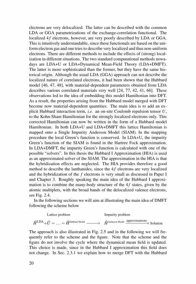
In the following sections we will aim at illustrating the main idea of DMFT

following the scheme below

Lattice problem Impurity problem

HLDA+U = . . .= HHubbard Model −−−−→ HAnderson Model approximations−−−−−−−−→ Solution

The approach is also illustrated in Fig. 2.5 and in the following we will fre-

quently refer to the scheme and the figure. Note that the scheme and the

figure do not involve the cycle where the dynamical mean field is updated.

This choice is made, since in the Hubbard I approximation this field does

not change. In Sec. 2.3.1 we explain how to merge DFT with the Hubbard

20

Energy

Intensity

+ =

6s6p5d

Energy

Intensity

4f

Energy

Intensity

4f

6s6p5d

Figure 2.4. The idea of the Hubbard I approximation is to combine the LDA (GGA)

description of the delocalized conduction electrons (light blue density of states) with

the atomic multiplets of the localized 4 f electrons (green solid multiplets).

model. In Sec. 2.3.2 the mapping procedure to the SIAM is explained. Finally

we explain how the Hubbard I approximation is implemented in RSPt [97]

in Sec. 2.3.3. The following sections are based mainly on the introductory

lectures of Antoine Georges [33] and the PhD thesis of Igor Di Marco [27].

Figure 2.5. In the Hubbard I approximation the lattice problem is mapped to an impu-

rity problem which is simplified into an atomic problem.

2.3.1 Effective Hubbard model

In this section we show how the Hubbard model is merged with DFT. This is

the blue part (left) of the illustrating scheme introduced previously



The LDA+DMFT approach is based on the idea of merging LDA and the

Hubbard model. In a heuristic way, one adds a Hubbard interaction term to

the DFT-LDA Hamiltonian for those orbitals where the description in LDA

21

is not good enough due to strong on-site Coulomb repulsion. The adjusted

Hamiltonian reads

HHUB = ∑Ri,R jχi,χ j

HLDARi,R jχi,χ j

c†Riχi

cR jχ j+

1

2∑R

∑ξ1,ξ2,ξ3,ξ4

Uξ1ξ2ξ3ξ4c†Rξ1

c†Rξ2

cRξ4cRξ3

−∑R

HDCR ,

(2.7)

where the LDA Hamiltonian is projected onto one-particle site-centered or-

bitals labeled by the Bravais lattice site vector R and the set of quantum num-

bers χ . The orbitals for which the local correction tensor U is added, are usu-

ally called the “correlated orbitals”. This set of orbitals is labeled by a general

orbital index ξ . Later on we will split ξ in more well-known quantum num-

bers, but in principle other classifications can be used. In an atomic-like basis

this would correspond to the spin-orbitals {l,m,σ}. The operators c†R and cR

are the creation and annihilation operators for electrons in the site-centered

or the correlated orbitals. Some of the correlation effects explicitly added by

the interaction term U are already (wrongly) taken into account in the LDA

Hamiltonian. The double counting term HDCR corrects for this by subtracting

these contributions from HHUB. This term has the form HDCR ∼ ∑ξ1

c†Rξ1

cRξ1

and is sometimes merged with the chemical potential. We will elaborate more

on this term in Fig. 2.7 and Sec. 2.3.5, but for the moment let us ignore it.

Written in this form, the corrected LDA Hamiltonian HHUB can be viewed

as a Hubbard model Hamiltonian. The hopping term

tR1χ1,R2χ2= HLDA

R1,R2χ1,χ2

=∫

dr〈R1χ1|r〉 HLDA(r)〈r|R2χ2〉 (2.8)

comes from the LDA problem and the on-site repulsive interaction U is added

on top of that. Note, however, that U is not the bare Coulomb repulsion, but an

effective interaction. This effective interaction is based on the Coulomb repul-

sion, but is screened by the other electrons. We will discuss the heuristically

added U-tensor in Sec. 2.3.4.

2.3.2 Effective Single impurity Anderson model

Now that we have a material-dependent Hubbard model Hamiltonian time has

come to solve it. An efficient way to obtain physical quantities from this

Hamiltonian is provided by the dynamical mean-field theory. In DMFT the

effective Hubbard model, introduced in Sec. 2.3.1, is mapped onto an effec-

tive model, the single impurity Anderson model (SIAM). The SIAM considers

a single impurity embedded in an effective field, as illustrated in the middle

of Fig. 2.5. This way of solving the Hubbard model corresponds to solving

the problem in a mean-field approach for the space degrees of freedom. The

quantum degrees of freedom at a single site are, however, still accounted ex-

actly. The mapping procedure is highlighted in the second part of the scheme

22

below


HLDA+U = . . .= HHubbard Model−−−−→ HAnderson Model approximations−−−−−−−−→ Solution

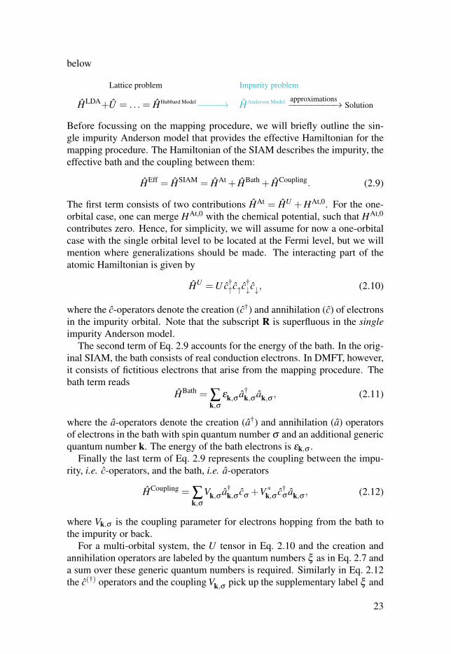
Before focussing on the mapping procedure, we will briefly outline the sin-

gle impurity Anderson model that provides the effective Hamiltonian for the

mapping procedure. The Hamiltonian of the SIAM describes the impurity, the

effective bath and the coupling between them:

HEff = HSIAM = HAt + HBath + HCoupling. (2.9)

The first term consists of two contributions HAt = HU +HAt,0. For the one-

orbital case, one can merge HAt,0 with the chemical potential, such that HAt,0

contributes zero. Hence, for simplicity, we will assume for now a one-orbital

case with the single orbital level to be located at the Fermi level, but we will

mention where generalizations should be made. The interacting part of the

atomic Hamiltonian is given by

HU =U c†↑c↑c

†↓c↓, (2.10)

where the c-operators denote the creation (c†) and annihilation (c) of electrons

in the impurity orbital. Note that the subscript R is superfluous in the singleimpurity Anderson model.

The second term of Eq. 2.9 accounts for the energy of the bath. In the orig-

inal SIAM, the bath consists of real conduction electrons. In DMFT, however,

it consists of fictitious electrons that arise from the mapping procedure. The

bath term reads

HBath = ∑k,σ

εk,σ a†k,σ ak,σ , (2.11)

where the a-operators denote the creation (a†) and annihilation (a) operators

of electrons in the bath with spin quantum number σ and an additional generic

quantum number k. The energy of the bath electrons is εk,σ .

Finally the last term of Eq. 2.9 represents the coupling between the impu-

rity, i.e. c-operators, and the bath, i.e. a-operators

HCoupling = ∑k,σ

Vk,σ a†k,σ cσ +V ∗k,σ c†

σ ak,σ , (2.12)

where Vk,σ is the coupling parameter for electrons hopping from the bath to

the impurity or back.

For a multi-orbital system, the U tensor in Eq. 2.10 and the creation and

annihilation operators are labeled by the quantum numbers ξ as in Eq. 2.7 and

a sum over these generic quantum numbers is required. Similarly in Eq. 2.12

the c(†) operators and the coupling Vk,σ pick up the supplementary label ξ and

23

the summation extends also over this generic quantum number. Additionally

the term HAt,0 in HAt in Eq. 2.9 is required to account for the energy of the

impurity electrons:

HAt,0 = ∑ξi,ξ j

εξiξ jc†

ξicξ j

, (2.13)

where the energy of the impurity electrons is obtained from the LDA Hamil-

tonian projected onto the correlated orbitals. As said, for the remainder of the

explanation of the SIAM, we focus on the single impurity Anderson model

with the impurity level positioned at zero.

In DMFT the mapping of the Hubbard model to the Single Impurity Ander-

son model is done such that the local Green’s function at a single site in the

lattice problem is the same as the impurity Green’s function of the effective

SIAM. To achieve this, the mapping parameters εk,σ and Vk,σ should be set

correctly. In reality these parameters are not needed explicitly. We will see

in the following that only the dynamical field Δσ should be found. The local

Green’s function at a single site in the lattice problem is defined as a function

of the creation and annihilation operators in the lattice problem. In DMFT the

focus is on the correlated orbitals ξ and the local Green’s function for these

orbitals reads:

GLocRR,σξ1ξ2

(τ− τ ′)≡−〈TcRξ1σ (τ)c†Rξ2σ (τ

′)〉 , (2.14)

where T denotes the time ordering operator and τ the imaginary time in the

Matsubara formalism. If τ > τ ′, an electron is created in orbital ξ2 by c†Rξ2σ (τ

′)at time τ ′, it propagates through the system until it is annihilated at time τin orbital ξ1 by cRξ1σ (τ). On the other hand, if τ ′ > τ , a hole is created in

orbital ξ1 by cRξ1σ (τ) which propagates until it is annihilated in orbital ξ2

by c†Rξ2σ (τ

′). In the SIAM, the impurity Green’s function is defined as the

Green’s function associated to the impurity operators c in Eqs. 2.10, 2.12

and 2.13. The impurity Green’s function reads:

GImp

ξ1ξ2σ (τ− τ ′)≡−〈Tcξ1σ (τ)c†ξ2σ (τ

′)〉 . (2.15)

In order to find the mapping parameters εk,σ and Vk,σ , it is convenient to

split this impurity Green’s function into a non-interacting impurity Green’s

function and a self-energy that contains the interactions. To obtain the non-

interacting part, the term in Eq. 2.10 is equated to zero. The following expres-

sion for the non-interacting part of the impurity Green’s function can be found

either by using the effective action functional integral formalism and integrat-

ing out the bath degrees of freedom [33], or by using the equations of motion

for the c and a operators [84]. The non-interacting impurity Green’s function

then reads:

G Imp,0σ =

[(iωn +μ)1− HAt,0−Δσ (iωn)

]−1, (2.16)

24

where Δσ is the hybridization function that contains the parameters εk,σ and

Vk,σ of the effective system

Δσ (iωn) = ∑k

|Vk,σ |2iωn− εk,σ

. (2.17)

With this, we can formally rewrite the effect of the two-particle term contained

in HU in the form of a self-energy function ΣImpσ (iωn). This function can

be determined by several techniques, named “solvers”. The Dyson equation

relates the interacting Green’s function to the non-interacting Green’s function

and the self-energy:

GImpσ (iωn) =

[(G Imp,0

σ (iωn))−1−ΣImp

σ (iωn)

]−1

. (2.18)

In DMFT, the approximation is made that the lattice self-energy is local or in

other words k-independent. With this approximation, the lattice self-energy

can be directly related to the impurity self-energy

ΣRR′,σ (iωn) = δRR′ΣImpσ (iωn). (2.19)

There are three limiting cases where the DMFT approximation is exact. The

first case is trivial and is the non-interacting limit. If U = 0, the self-energy is

zero and thus trivially local. The second exact limit was proven by Metzner

and Vollhardt [69] who showed that the DMFT approximation is exact in the

limit of infinite nearest neighbors or infinite dimensions. The third limit is the

atomic limit, where the hopping between nearest neighbors in Eq. 2.8 of the

Hubbard model becomes zero tR1,χ1,R2,χ2∼ δR1,R2

. This results in Δσ (iωn) = 0

which implies a self-energy that has only on-site components. The Hubbard I

approximation, which is an approximate solver to the SIAM in DMFT, is build

upon this limit. It involves an additional approximation on top of the DMFT

approximation that can be viewed in different ways. In the Hamiltonian of

the effective system, i.e. Eq. 2.9, the coupling between the bath and the im-

purity, is neglected. For the self-energy this boils down to approximating the

self-energy in the impurity problem by the atomic self-energy. Using this ap-

proximate solver for DMFT results in a lattice self-energy that is approximated

by the atomic self-energy

ΣRR′,σ (iωn) = δRR′ΣAtσ (iωn). (2.20)

The above described procedure, where the Hubbard model (Eq. 2.7) is mapped

onto the single impurity Anderson model (Eq. 2.9) and then approximated

by an atomic problem is schematically depicted in Fig. 2.6, which is an ex-

tended version of Fig. 2.5. The mapping procedure is no longer exact. In full

DMFT, one has to find εk,σ and Vk,σ and the resulting hybridization function

25

Δ and self-energy Σ that reproduce the correct GImpσ , such that GImp

σ (iωn) =GLoc

σ (iωn). This is the core ingredient of the mapping procedure in full DMFT.

In the HIA, however, the hybridization function is neglected and the atomic

self-energy is taken instead of the true self-energy. Hence, the hybridization

function needs not to be found self-consistently. The crucial approximation

(Vk,σ = 0) is made and this method can only give sensible results if the corre-

lated orbitals are close to atomic-like. Or, in other words, if the hybridization

is very small. In this thesis we only mention the Hubbard I Approximation as

an approximate solver for the SIAM in DMFT, since it is a good approxima-

tion for the rare earths. However, there are several other possible solver that

are appropriate for other particular cases. In the scheme that was leading in

this section, the solvers are the last part:



Figure 2.6. In the Hubbard I approximation the lattice problem is mapped to an impu-

rity problem which is simplified into an atomic problem. The self-energy is calculated

in the simplified case and the real self-energy is approximated by the atomic self-

energy.

2.3.3 Computational scheme

In Paper I we thoroughly investigated the Hubbard I approximation for the

elemental rare-earth metals and in Paper II we used this HIA to support the

calculations done with the 4 f -in-the-core method. In this section we briefly

outline the computational scheme of HIA that we used in these works, i.e. the

HIA implementation in the RSPt code [97].

As a guidance to the reader, we sketched the computational scheme for the

Hubbard I approximation in Fig. 2.7. First the Kohn-Sham Hamiltonian HLDA

26

Figure 2.7. Outline of the HIA cycle. The symbols are explained in the text.

27

coming from the DFT-LDA part in a global basis χ is projected onto the corre-

lated states denoted with a generic set of quantum numbers ξ on site R. In case

of the lanthanides, HLDA is projected onto the atomic-like 4 f states. This is

Eq. 2 in Fig. 2.7 or Eq. 2.13 in the previous section. The resulting Hamiltonian

HAt,0R is written on a many-body basis of Fock states and the on-site Coulomb

repulsion tensor U (Eq. 2.10 in the previous section) is added. The resulting

HAtR in Eq. 3 in Fig. 2.7 also contains the terms (μ+ΔμAt+μDC) that take into

account the chemical potential of the Green’s function coming in the first itera-

tion from the LDA calculation, the correction due to the fact that the hybridiza-

tion is ignored in the HIA and the double counting correction. In Sec. 2.3.5

we will elaborate a bit more on these terms. This Hamiltonian is diagonalized

and the eigenvalues Eν and the eigenstates |ν〉 are obtained. With the Lehman

representation, the interacting atomic Green’s function GAt (Eq. 5 in Fig. 2.7)

is constructed. Meanwhile the non-interacting atomic Green’s function is con-

structed from HAt,0R . The non-interacting Green’s function GAt,0 and the in-

teracting Green’s function GAt combined with the Dyson equation provide the

atomic self-energy ΣAt in Eq. 7 of Fig. 2.7. The self-energy includes, as usual,

the interactions of the system. The Hubbard I approximation consists in ap-

proximating the impurity self-energy with the atomic self-energy, as is done

in Eq. 8 in Fig. 2.7. To return back to the lattice problem, the self-energy has

to be up-folded to the global basis as in Eq. 2.19 or 2.20 in the previous sec-

tion. This self-energy in the global basis is used to construct the one-electron

Green’s function in the global basis, as is shown in Eq. 9 in Fig. 2.7. Here the

atomic features and the delocalized electrons are combined. The chemical po-

tential μ is adjusted to get the right amount of particles. To allow the itinerant

electrons to adjust to the changed potential of the correlated electrons, charge

self-consistency is required. The density of the delocalized electrons has to

be recalculated taking the new density of the localized electrons into account.

This results in a slightly different HLDA in Eq. 1 in Fig. 2.7. The loop has to

be repeated until the density and the self-energy do not change significantly

anymore between consecutive iterations.

The most important physical properties can be obtained through the lattice

Green’s function. A fundamental quantity to calculate is the spectral function,

which is given by

ρ(ω) =− 1

πIm [G(ω + iδ )] δ → 0, (2.21)

where δ approaches 0 from the positive side. In computations δ will never be

exactly zero and causes therefore a broadening in the spectrum.

2.3.4 Hubbard U and Hund’s JIn this section we will elaborate on the U tensor and its relation to the Hubbard

U and Hund’s J. In our code we work directly with the full U-tensor. Because

28

of the atomic-like orbitals, the U-tensor can be expanded with help of spherical

harmonics. The expansion [20, 27] is given by

Um1σ1,m2σ2,m3σ3,m4σ4= δσ1,σ3

δσ2,σ4

2l

∑n=0

an(m1,m3,m2,m4)Fn, (2.22)

where the δ s ensure that the interaction does not change the spin of the elec-

trons. The parameters an are integrals over products of three spherical har-

monics. Their form is such that they are only non-zero if n is even and n≤ 2l.The Slater integrals Fn are given by

Fn =∫ ∞

0

∫ ∞

0drdr′r2r′2|φ(r)|2|φ(r′)|2 rn

<

rn+1>

, (2.23)

where φ are the atomic radial wave functions and r< and r> denote the lesser

and the greater between r and r′. The zeroth Slater integral is heavily screened.

This means that a direct evaluation of Eq. 2.23 to obtain F0 is nonsensical.

However, for F2, F4 and F6 the screening is much smaller and the atomic

Slater integrals are already very good approximations. Using the atomic F2,

F4 and F6 has the advantage of not introducing an additional parameter to

account for the small screening of these Slater integrals.

In our code we use the full U-tensor to calculate the self-energy. However,

in Paper I and Paper II we frequently refer to the Hubbard U and Hund’s J.

These parameters are useful for an intuitive understanding of the effects of

adding the U tensor to the Hamiltonian. In the remainder of this section we

briefly comment on the physical meaning of the Hubbard U and Hund’s J.

For this, we consider two degenerate correlated orbitals in cubic symmetry

described by real valued wave functions. In this case, the Coulomb interaction

tensor can be rewritten as [44]:

1

2∑

ξ1,ξ2,ξ3,ξ4

Uξ1,ξ2,ξ3,ξ4c†

ξ1c†

ξ2cξ4

cξ3

−→ 1

2∑m,σ

Unmσ nmσ +1

2∑

m,m′,σ ,σ ′m�=m′

((U−2J)nmσ nm′σ ′ − Jnmσ nm′σ )

− 1

2∑

m,m′,σm�=m′

J(

c†mσ c†

mσ cm′σ cm′σ + c†mσ cmσ c†

m′σ cm′σ

). (2.24)

In this equation the general quantum number ξ of the correlated orbitals is

split in a principal quantum number n, an angular quantum number l, an or-

bital quantum number m, and a spin quantum number σ . The principal quan-

tum number and the angular quantum number subscripts are ignored since we

consider all correlated orbitals to have the same n and l. Note that n = c†c is

29

the number operator and σ is a spin opposite to σ . The Hubbard U and Hund’s

J are parts of the Coulomb interaction tensor

U =Ummmm Intraorbital interaction

U−2J =Umm′mm′ with m �= m′ Interorbital interaction (2.25)

J =Umm′m′m with m �= m′ Pair-hopping amplitude or exchange interaction.

The precise derivation of these relationships is not relevant here, since we only

use Eq. 2.24 for an intuitive understanding of these parameters. The interested

reader is referred to Refs. [44, 32, 62]. The meaning of U and J for the two-

orbital system is illustrated in Fig. 2.8. This figure is a schematic view of a

system consisting of two degenerate orbitals at zero energy and initially one

electron in orbital 1. The question is, what is the energy cost to add 1 electron

to this system? We could add this second electron in three ways and the energy

cost ΔE can be found by applying the Hamiltonian in Eq. 2.24 to the initial

Figure 2.8. Schematic view of how the Hubbard U and Hund’s J shift the “energy lev-

els". Energy levels are an intuitive way of understanding these numbers, but are a bit

difficult to grasp in case of a many-body state. For simplicity we take two degenerate

orbitals at zero energy. In the initial case we have one electron and two orbitals. In

the final case, we have two electrons and a many-body state, which might be a sort

of combination between the original two orbitals. This combination is denoted with a

wiggly line between the orbitals. The position of the many-body orbital is such that,

in order to obtain the energy of the system, you have to take the energy of the energy

level times the occupancy of the level. The most left plots correspond to the initial sit-

uation with one electron in orbital 1. In the second column an electron with opposite

spin is added to the second orbital. In the third column an electron with opposite spin

is added to the same orbital and in the last column an electron with same spin is added

to (of course) the other orbital. The top panels show the shift of the energy levels in the

situation where the Coulomb repulsion is taken into account. The bottom panels show

the situation where it is not taken into account, so the independent electron theory.

30

state and the final state. We neglected the terms in the last line of Eq. 2.24

which are considered to be small. This results in the following three possible

energy costs for adding an electron

1. With opposite spin in the 2nd orbital: ΔE = U122 + U21

2 =U−2J2. With opposite spin in the same orbital: ΔE = U11

2 + U112 =U

3. With the same spin in the 2nd orbital: ΔE = U12−J122 + U21−J21

2 =U−3JThese energy costs are illustrated in Fig. 2.8.

The preceding discussion offers an idea of the different contributions to the

U-matrix, but several approximations have been performed. These approxi-

mations where only made to simplify the understanding of the physics. In our

code we use the full U-tensor to calculate the self-energy. The different Slater

integrals are related by sum rules [20, 27] and can therefore be related to the

Hubbard U and Hund’s J. The former corresponds to the zeroth Slater integral

F0 =U and is usually heavily screened. The Hund’s J for f systems is given

by J = 16435(286F2 +195F4 +250F6) [20, 27].

2.3.5 Double counting

Finally we return to HDC in Eq. 2.7, which contains the last terms in Eq. 3of Fig. 2.7, i.e. (μ +ΔμAt + μDC). The first term μ is simply the chemi-cal potential obtained from the DFT-LDA calculation in the first iteration. Incharge self-consistent calculations it will be modified to account for the self-energy. The last term μDC is more tricky. As mentioned before the U-tensoris added to take into account the strong Coulomb interaction in the localizedorbitals. However, part of this Coulomb repulsion is already accounted for inthe DFT-LDA calculation, although not correctly. The double counting termμDC should correct for this. Moreover, in HIA, we neglect the coupling be-tween impurity and bath, when mapping the electronic structure problem ontothe SIAM. The term ΔμAt should in principle enforce the conservation of theparticle number between the SIAM and the atomic model obtained in HIA.However in practice this is not needed. These two terms ΔμAt and μDC havein common that they are rigid shifts. Therefore they are sometimes groupedtogether into one term. Unfortunately it is not straightforward to know whichcontributions are exactly double counted and hence the choice of the double-counting correction is a somewhat arbitrary procedure. Several schemes forthe double counting have been proposed and used in different situations. InTab. 2.1 we summarize the double-counting schemes relevant for the HIA andused in the Papers I and II. We will explain them briefly below.

Fix position of the first (un)occupied peakThis scheme acknowledges the fact that we do not know the exact expres-

sion for the double counting and introduces an additional parameter to fix this

lack of knowledge. This scheme is very convenient when comparing with ex-

perimental photoemission spectra. In this procedure, the position of the first

occupied or the first unoccupied peak from theory is aligned to the position

31

Table 2.1. Double counting corrections

Double counting scheme Input Determines

Position of the first NAt, EPeak (ΔμAt +μDC) = HDC(NAt,EPeak)(un)occupied peak μ is determined self-consistently

Fully Localized Limit (N) μDC +ΔμAt = HDC(N)μ is determined self-consistently

Fully Localized Limit (NAt) NAt μDC +ΔμAt = HDC(NAt)μ is determined self-consistently

of this peak obtained in experiment, which has to be given as an external pa-

rameter. This allows for an easy comparison of the relative positions of the

atomic multiplets. This double-counting correction is implemented such that

once μ has been determined to obtain the correct number of electrons in the

global system, ΔμAt + μDC is adjusted to get the correct number of f elec-

trons. Since the multiplets are well separated in energy, ΔμAt + μDC is still

undetermined within this range. Fixing the position of the first (un)occupied

peak to the experimental position determines ΔμAt +μDC univocally.

Fully localized limitA legitimate protest against the previously described scheme is that introduc-

ing an additional parameter is not very ab-initio. The fully localized limit

(FLL) double counting is an approximation that is without external parame-

ters and that is frequently used together with the HIA. In the fully localized

limit, the double counting energy is given by

EDC =1

2UN(N−1)− J

N2

(N2−1

), (2.26)

where N is the number of correlated electrons as calculated from the local

Green’s function. Alternatively one could choose the closest integer number

to N instead [82]. The latter we label NAt and is very close to N for a true

Hubbard I system.

The double counting Hamiltonian in Eq. 2.7, which is diagonal in ξ ,ξ ′, is

obtained through:

HDCR,ξ ,ξ ′ =

{δEDC

δ nRξif ξ = ξ ′,

0 if ξ �= ξ ′.(2.27)

32

3. Lanthanides

The rare earths perplex us in our researches, baffle us in our speculations,and haunt us in our very dreams. They stretch like an unknown sea before us,

mocking, mystifying, and murmuring strange revelations and possibilities.

— Sir William Crookes (1887)

THE lanthanides, which are the elements from Ba/La to Lu, or rare-

earth (RE) elements1 have very interesting properties, such as their

large magnetic moment and anisotropy. Many of the characteristics

of the REs arise from the very localized nature of the 4 f electrons.

The standard model of the lanthanides, which assumes a chemically inert 4 fshell and 4 f orbitals that are very close to atomic like, has been proven to

work very well to describe and explain experimental findings. However, it

has been difficult to connect ab initio electronic structure calculations to this

model. Density functional theory, with the commonly used parameterizations

of the exchange correlation functional (LDA/GGA), badly fails to correctly

describe the localized nature of the 4 f electrons and therefore most properties

of the REs. More sophisticated theories have been tried, such as LDA+U [4],

self-interaction correction (SIC) [81], orbital polarization [30], and a treat-

ment of the 4 f shell as core-like [88]. All these methods can describe certain

properties very well, but fail to provide a unified picture of the physics of the

REs. Especially a correct description of the valence band spectra is not within

the possibilities of these methods. In Paper I we study density functional the-

ory plus dynamical mean-field theory (DFT+DMFT) within the Hubbard I

approximation (HIA) to describe a wide range of properties of the REs.

In this chapter we will provide a background to some of these properties.

On the one hand this is a good introduction to Paper I and II, on the other hand

it intuitively shows why the standard model of the lanthanides is so success-

ful. We will focus in Sec. 3.1 on the electronic configuration of the REs, since

all physical properties originate from this. In Sec. 3.2 we will describe the

bonding properties of the REs. In Sec. 3.3 we mention the crystal structure of

the elemental RE metals and discuss the phase diagram of cerium as a back-

ground to Paper II. We will continue in Sec. 3.4 with the ground-state magnetic

moments of the lanthanides, which are very close the the atomic Hund’s rule

1The rare-earth elements also include Sc and Y, which are not part of the lanthanide series.

However, I use the term rare earths synonymously to lanthanides in this thesis.

33

derived moments. Finally we arrive at the valence-band (inverse) photoemis-

sion spectra in Sec. 3.5. This introduction to the rare earths is largely based on

Chapter 2 of my licentiate thesis [62].

At the end of this chapter we will summarize Paper I and II. In Paper I

is shown how accurately DFT+DMFT within HIA can describe the different

properties of the elemental rare earths. In Paper II we use this method to

calculate the stacking fault energies of γ-cerium.

3.1 Outer electronic configurationAcross the lanthanides the 4 f shell is gradually filled. The electronic config-

uration of an isolated atom with n electrons in the 4 f shell is [Xe]6s25d04 f n,

except for La, Gd and Lu that have a 5d electron more and one 4 f electron

less [7]. When the isolated atoms come together and form a solid, the discrete

6s, 6p and 5d energy levels hybridize into an [spd] band. A balance is found

between the Coulomb energy to pay when adding a localized f electron and

the kinetic energy to pay when adding an itinerant [spd] electron. For most

REs it is energetically favorable to promote one 4 f electron to the [spd]-band

in the solid phase, which results in three [spd] valence electrons. The excep-

tions to this are barium, europium and ytterbium that have an empty, half filled

or filled shell in the atomic configuration. The Coulomb energy to pay when

adding an f electron to obtain a half-filled or full shell is very small. These

elements, with two [spd] valence electrons are called divalent contrary to the

other trivalent elements. In the following table the outer electronic config-

uration of the rare earths is given for the atomic (A) and the crystalline (C)

phases.

La Ce Pr Nd Pm

A 5d16s2 4 f 25d06s2 4 f 35d06s2 4 f 45d06s2 4 f 55d06s2

C [spd]3 4 f 1[spd]3 4 f 2[spd]3 4 f 3[spd]3 4 f 4[spd]3

Sm Eu Gd Tb Dy

A 4 f 65d06s2 4 f 75d06s2 4 f 75d16s2 4 f 95d06s2 4 f 105d06s2

C 4 f 5[spd]3 4 f 7[spd]2 4 f 7[spd]3 4 f 8[spd]3 4 f 9[spd]3

Ho Er Tm Yb Lu

A 4 f 115d06s2 4 f 125d06s2 4 f 135d06s2 4 f 145d06s2 4 f 145d16s2

C 4 f 10[spd]3 4 f 11[spd]3 4 f 12[spd]3 4 f 14[spd]2 4 f 14[spd]3

3.2 Bonding propertiesThe equilibrium atomic volumes of the elemental RE metals, i.e. crystals

consisting of only one type of RE atoms, very intuitively show how the local-

34

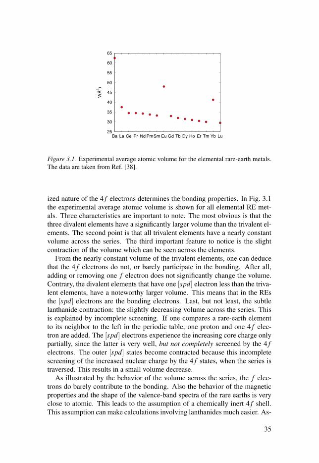
25

30

35

40

45

50

55

60

65

Ba La Ce Pr Nd PmSm Eu Gd Tb Dy Ho Er Tm Yb Lu

V(Å3 )

Figure 3.1. Experimental average atomic volume for the elemental rare-earth metals.

The data are taken from Ref. [38].

ized nature of the 4 f electrons determines the bonding properties. In Fig. 3.1

the experimental average atomic volume is shown for all elemental RE met-

als. Three characteristics are important to note. The most obvious is that the

three divalent elements have a significantly larger volume than the trivalent el-

ements. The second point is that all trivalent elements have a nearly constant

volume across the series. The third important feature to notice is the slight

contraction of the volume which can be seen across the elements.

From the nearly constant volume of the trivalent elements, one can deduce

that the 4 f electrons do not, or barely participate in the bonding. After all,

adding or removing one f electron does not significantly change the volume.

Contrary, the divalent elements that have one [spd] electron less than the triva-

lent elements, have a noteworthy larger volume. This means that in the REs

the [spd] electrons are the bonding electrons. Last, but not least, the subtle

lanthanide contraction: the slightly decreasing volume across the series. This

is explained by incomplete screening. If one compares a rare-earth element

to its neighbor to the left in the periodic table, one proton and one 4 f elec-

tron are added. The [spd] electrons experience the increasing core charge only

partially, since the latter is very well, but not completely screened by the 4 felectrons. The outer [spd] states become contracted because this incomplete

screening of the increased nuclear charge by the 4 f states, when the series is

traversed. This results in a small volume decrease.

As illustrated by the behavior of the volume across the series, the f elec-

trons do barely contribute to the bonding. Also the behavior of the magnetic

properties and the shape of the valence-band spectra of the rare earths is very

close to atomic. This leads to the assumption of a chemically inert 4 f shell.

This assumption can make calculations involving lanthanides much easier. As-

35

Figure 3.2. Top view of a close-packed lattice. If the first layer is formed by the green

atoms, site A, the second layer can be placed at site B (blue) or site C (yellow). The

order of the stacking determines the crystal structure.

Figure 3.3. Side view of the different close-packed stacking orders. The order of the

stacking determines the crystal structure.

suming a chemically inert 4 f -shell is often denoted as the standard model of

the lanthanides.

3.3 Structural stabilities

Also for the crystal structure of the RE metals, the localized nature of the

4 f electrons is decisive. Since the 4 f shell is very localized, the change in

4 f filling barely modifies the outer regions of the atom. This means that all

RE metals, except the divalent ones, have very similar properties, as we have

already seen for the equilibrium volume in Sec. 3.2. The crystal structures

of the trivalent elements are from light to heavy: fcc (Ce) → dhcp (Pr,Nd) →Sm-structure (Sm)→ hcp (Gd-Tm) [52], which are all close-packed structures

with different stacking of a layer where the atoms are arranged in triangles, see

Fig. 3.2. The order of the stacking determines the crystal structure as shown

in Fig. 3.3 for the crystal structures of the RE metals. The structural phase

diagrams of the RE metals are also very similar, as they all go through the

following sequence with increasing pressure hcp → Sm-structure → dhcp →fcc. This inspired B. Johansson and A. Rosengren [52] to compile a gener-

alized phase diagram for all elemental RE metals. In Paper I we address the

36

structural stabilities of Ce, Pr and Nd. In Paper II we also look in detail at

the different crystal phases of Ce, maybe the most intensively studied material

amongst the elemental RE metals. Precisely this element does not entirely fit

in the generalized phase diagram. Instead of the expected dhcp phase for low

temperatures and pressures, an fcc structure is found. Around room temper-

ature and only for low pressures, a small dhcp region is found and for higher

temperatures Ce takes again an fcc structure [99]. However, the most interest-

ing feature in the Ce phase diagram is the transition from the low pressure fcc

(γ-) phase to the high pressure fcc (α-) phase. This is an isostructural transi-

tion with a dramatic volume collapse of about 15% around room temperature.

Also the spectral weight changes from the γ- to the α-phase [44]. We will

return to this phase diagram in Sec. 3.6 and Fig. 3.9.

In Paper II we study the energies of the different crystal phases. These

energy differences are quite small, i.e. only tens of meV. From the energies

of the different hexagonal stacking orders (Fig. 3.3) we calculate the stacking

fault energies by using the axial interaction model [26, 21]. The stacking fault

energies are quite small and errors in the stacking fault are relatively easily

formed. The difference in the stacking fault energy in the γ and α phase gives

insight in the hysteretic effects in the α-γ transition.

3.4 MagnetismIn this section we will briefly describe the ground-state magnetic moments

of the REs. For the present we keep it simple and neglect crystal-field ef-

fects. Although, we will present a basic picture without crystal-field effects,

for some of the rare earths, like Pr, they are extremely important. More specif-

ically we will describe the coupling of spin and orbital moments as encoded

in Hund’s rules and the Russell-Saunders coupling scheme. In the end we will

mention the paramagnetic moment and the saturation moment that are found

in small and big fields respectively. For this section, and for my knowledge of

magnetism in the REs, Solid State Physics by Ashcroft and Mermin [7], Rareearth Magnetism by Jensen and Mackintosh [51] and the Master’s Thesis of

N.E. Koch [53] were very useful.

3.4.1 Coupling of spin and orbital moments

The moments of the rare earths are well described in the Russell-Saunders

(LS) coupling scheme, which is based on the assumption that spin-spin cou-

pling is stronger than orbit-orbit coupling, which is stronger than spin-orbit

coupling. The exchange interaction couples the spins si of the individual elec-

trons to a total spin angular momentum S, with total spin quantum number

S = ∑i mis where mi

s is the spin projection quantum number of electron i. Sim-

ilarly, the Coulomb interaction couples the orbital angular momenta li of the

37

individual electrons to a total orbital angular momentum L. The correspond-

ing total orbital angular momentum quantum number is L = ∑i mil , where the

magnetic quantum number mil specifies the projection of the orbital angular

momentum of electron i along the quantization axis. These two couplings are

summarized in Hund’s first two, out of three, rules. These three Hund’s rules

make it possible to find the ground state:

1. Maximize S, taking into account the Pauli principle.

2. Maximize L, while satisfying the first rule.

3. Minimize J for less than half filled shells (J = |L−S|) or maximize J for

more than half filled shells (J = |L+ S|), while satisfying the first two

rules.

The third Hund’s rule describes the coupling of the spin and orbital angular

momentum into the total angular momentum J. The corresponding total angu-

lar momentum quantum number is given by J = |L±S|. The spin and orbital

angular momenta are subtracted for less than half filled shells, since the en-

ergy is smallest for the state where Sz = S and Lz = −L have opposite sign.

Contrary for more than half filled shells, where the energy is smallest when

Sz = S and Lz = L have the same sign. In this case the spin and orbital angu-

lar momenta have to be added in order to obtain the total angular momentum

quantum number. Here and from now on we indicate the quantization axis as

the z-axis for sake of simplicity.

3.4.2 Moments arising from the spin, orbital and total angularmomenta

The moments associated to the spin and orbital angular momenta combine to

a moment associated to the total angular momentum vector. The spin moment

is:

μμμS =−gsμB

hS, (3.1)

with gyromagnetic factor of the electronic spin gs ≈ 2 and Bohr magneton

μB. The magnitude of this moment is μS = gsμB

√S(S+1)≈ 2μB

√S(S+1),

where we used that the eigenvalues of S2 are h2S(S+ 1). The magnitude of

the orbital moment is

μL = μB

√L(L+1), (3.2)

which is also directed opposite to L. Note that the gyromagnetic factor for the

orbital moment is gL = 1, which is why it does not appear in Eq. 3.2.

The coupled moment as a function of the total angular momentum J can be

written in a similar form

μJ = gJμB

√J(J+1), (3.3)

where the Landé factor gJ has a more complicated form, due to the factor two

in the spin moment that is not present in the orbital moment. The Landé factor

38

Figure 3.4. Vector representation of S, L and J, and the corresponding moments. The

vector representation is however a bit misleading, since we can not simultaneously

know all components of the vector.

is:

gJ = 1+J(J+1)+S(S+1)−L(L+1)

2J(J+1), (3.4)

which can be obtained as explained in the following. Fig. 3.4 illustrates in

a schematic way the “vector addition” of S, L to J and the addition of the

corresponding moments. As can be seen in Fig. 3.4 the sum of μμμS and μμμLdoes not lie along J, which is the unit vector in the J-direction. However, due

to the Wigner-Eckart theorem, the expectation value 〈μμμL +μμμS〉 should. The

total angular momentum J precesses around z, and the projection of μμμL +μμμSon the J-axis has length

μJ =μB

h

(L · J+2S · J) . (3.5)

Using L2 = (J− S)2 to obtain an expression for S · J and S2 = (J−L)2 to

obtain an expression for L · J leads to the gJ-factor in Eq. 3.4.

Note that we assumed that the field is not too strong so that S and L are

coupled to J. For strong fields, S and L would precess independently around

the direction of the external field.As a summary, the Hund’s rules ground state and the corresponding mag-

netic moments are listed in Tab. 3.1 for all rare earths. The ↑ and ↓ arrows in-dicate the ms occupation of the ml orbitals. The Hund’s rule ground state is, inzero field, (2J +1) fold degenerate and all states Jz =−J,−J +1, . . . ,J−1,Jhave the same energy. In the next section we will see how a magnetic fieldsplits this degeneracy. This leads to a magnetic moment that is different inweak or strong fields.

39

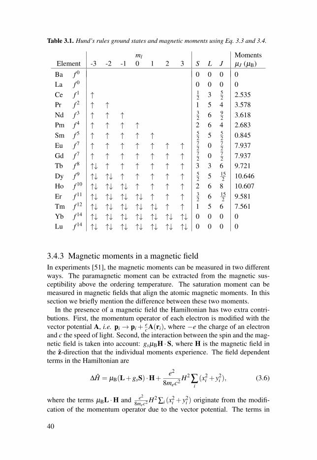
Table 3.1. Hund’s rules ground states and magnetic moments using Eq. 3.3 and 3.4.

ml Moments

Element -3 -2 -1 0 1 2 3 S L J μJ (μB)

Ba f 0 0 0 0 0

La f 0 0 0 0 0

Ce f 1 ↑ 12 3 5

2 2.535

Pr f 2 ↑ ↑ 1 5 4 3.578

Nd f 3 ↑ ↑ ↑ 32 6 9

2 3.618

Pm f 4 ↑ ↑ ↑ ↑ 2 6 4 2.683

Sm f 5 ↑ ↑ ↑ ↑ ↑ 52 5 5

2 0.845

Eu f 7 ↑ ↑ ↑ ↑ ↑ ↑ ↑ 72 0 7

2 7.937

Gd f 7 ↑ ↑ ↑ ↑ ↑ ↑ ↑ 72 0 7

2 7.937

Tb f 8 ↑↓ ↑ ↑ ↑ ↑ ↑ ↑ 3 3 6 9.721

Dy f 9 ↑↓ ↑↓ ↑ ↑ ↑ ↑ ↑ 52 5 15

2 10.646

Ho f 10 ↑↓ ↑↓ ↑↓ ↑ ↑ ↑ ↑ 2 6 8 10.607

Er f 11 ↑↓ ↑↓ ↑↓ ↑↓ ↑ ↑ ↑ 32 6 15

2 9.581

Tm f 12 ↑↓ ↑↓ ↑↓ ↑↓ ↑↓ ↑ ↑ 1 5 6 7.561

Yb f 14 ↑↓ ↑↓ ↑↓ ↑↓ ↑↓ ↑↓ ↑↓ 0 0 0 0

Lu f 14 ↑↓ ↑↓ ↑↓ ↑↓ ↑↓ ↑↓ ↑↓ 0 0 0 0

3.4.3 Magnetic moments in a magnetic field

In experiments [51], the magnetic moments can be measured in two different

ways. The paramagnetic moment can be extracted from the magnetic sus-

ceptibility above the ordering temperature. The saturation moment can be

measured in magnetic fields that align the atomic magnetic moments. In this

section we briefly mention the difference between these two moments.

In the presence of a magnetic field the Hamiltonian has two extra contri-

butions. First, the momentum operator of each electron is modified with the

vector potential A, i.e. pi → pi +ecA(ri), where −e the charge of an electron

and c the speed of light. Second, the interaction between the spin and the mag-

netic field is taken into account: gsμBH ·S, where H is the magnetic field in

the z-direction that the individual moments experience. The field dependent

terms in the Hamiltonian are

ΔH = μB(L+gsS) ·H+e2

8mec2H2 ∑

i(x2

i + y2i ), (3.6)

where the terms μBL ·H and e2

8mec2 H2 ∑i (x2i + y2

i ) originate from the modifi-

cation of the momentum operator due to the vector potential. The terms in

40

Eq. 3.6 induce energy shifts that are generally quite small and can be treated

with perturbation theory. For a state defined by the quantum numbers n ={J,L,S,Jz}, the energy shift is

ΔEn = μBH · 〈n|L+gsS|n〉+ ∑n′ �=n

| 〈n|μBH · (L+gsS)|n′〉 |2En−En′

+e2

8mc2H2 〈n|∑

ix2

i + y2i |n〉+ . . . (3.7)

We now focus on the case where J �= 0 in a small field in the z-direction. In this

case the first term in the above equation is usually dominant over the other two

which can be neglected. We assume that the separation between the zero field

ground-state multiplet, given by the Hund’s rules, and the first excited multi-

plet with a different J is much bigger than kBT and that only the (2J+1) states

within this ground-state multiplet will contribute to the moment. The energy

splitting, given in the above equation, then splits the (2J +1) fold degenerate

Hund’s rule ground state in states with Jz = −J,−J + 1, . . . ,J− 1,+J. The

(2J +1)-dimensional matrix 〈JLSJz|Lz +gsSz|JLSJ′z〉 can be simplified using

the Wigner-Eckart theorem

〈JLSJz|Lz +gsSz|JLSJ′z〉= g(JLS)JzδJzJ′z, (3.8)

where g(JLS) = gJ the same Landé gJ-factor as in Eq. 3.4. For clarity we

will skip the arguments (JLS) of the gJ-factor. Since Jz runs from −J to Jin integer steps, it follows from Eqs. 3.7 and 3.8 that the dominant energy

separation between the Jz levels in the ground-state J multiplet is gJμBH. The

paramagnetic and the saturation moment can be obtained in the case were

kBT � gJμBH and kBT � gJμBH respectively, as illustrated in the middle of

Fig. 3.5. In the following paragraphs we will calculate the paramagnetic and

the saturated moment.

Curie’s law kBT � gJμBHTo obtain the paramagnetic moment of a collection of identical atoms of an-

gular momentum J, one calculates the magnetic Helmholtz free energy F =− 1

β ln(Z ) for the excited states at energy En(H) = gJμBHJz, where Z is the

partition function. The exponentiated magnetic Helmholtz free energy is

e−βF = ∑n

e−βEn(H) =J

∑Jz=−J

e−βgJ μBHJz

=eβgJ μBH(J+1/2)− e−βgJ μBH(J+1/2)

eβgJ μBH/2− e−βgJ μBH/2. (3.9)

41

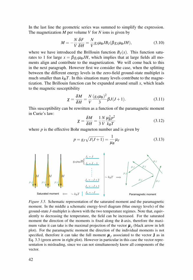
In the last line the geometric series was summed to simplify the expression.

The magnetization M per volume V for N ions is given by

M =−NV

δFδH

=NV

gJμBJBJ(βgJμBJH), (3.10)

where we have introduced the Brillouin function BJ(x). This function satu-

rates to 1 for large x = βgJμBJH, which implies that at large fields all mo-

ments align and contribute to the magnetization. We will come back to this

in the next paragraph. However first we consider the case, when the splitting

between the different energy levels in the zero-field ground-state multiplet is

much smaller than kBT . In this situation many levels contribute to the magne-

tization. The Brillouin function can be expanded around small x, which leads

to the magnetic susceptibility

χ =δMδH

=NV(gJμB)

2

3βJ(J+1). (3.11)

This susceptibility can be rewritten as a function of the paramagnetic moment

in Curie’s law:

χ =δMδH

=1

3

NV

μ2B p2

kBT(3.12)

where p is the effective Bohr magneton number and is given by

p = gJ√

J(J+1) =1

μBμJ (3.13)

Figure 3.5. Schematic representation of the saturated moment and the paramagnetic

moment. In the middle a schematic energy-level diagram (blue energy levels) of the

ground-state J-multiplet is shown with the two temperature regimes. Note that, equiv-

alently to decreasing the temperature, the field can be increased. For the saturated

moment the direction of the moments is fixed along the z-axis, therefore the maxi-

mum value it can take is the maximal projection of the vector μμμJ (black arrow in left

plot). For the paramagnetic moment the direction of the individual moments is not

specified, therefore it can take the full moment μμμJ associated to the vector J as in

Eq. 3.3 (green arrow in right plot). However in particular in this case the vector repre-

sentation is misleading, since we can not simultaneously know all components of the

vector.

42

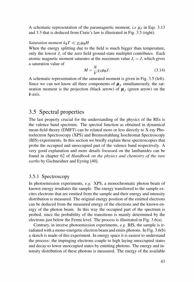
A schematic representation of the paramagnetic moment, i.e μJ in Eqs. 3.13

and 3.3 that is deduced from Curie’s law is illustrated in Fig. 3.5 (right).

Saturation moment kBT � gJμBHWhen the energy splitting due to the field is much bigger than temperature,

only the lowest Jz of the zero field ground-state multiplet contributes. Each

atomic magnetic moment saturates at the maximum value Jz = J, which gives

a saturation value of

M =NV

gJμBJ. (3.14)

A schematic representation of the saturated moment is given in Fig. 3.5 (left).

Since we can not know all three components of μμμJ simultaneously, the sat-

uration moment is the projection (black arrow) of μμμJ (green arrow) on the

z-axis.

3.5 Spectral properties

The last property crucial for the understanding of the physics of the REs is

the valence band spectrum. The spectral function as obtained in dynamical

mean-field theory (DMFT) can be related more or less directly to X-ray Pho-

toelectron Spectroscopy (XPS) and Bremsstrahlung Isochromat Spectroscopy

(BIS) experiments. In this section we briefly explain these spectroscopies that

probe the occupied and unoccupied part of the valence band respectively. A

very good explanation and more details focussed on the lanthanides can be

found in chapter 62 of Handbook on the physics and chemistry of the rareearths by Gschneidner and Eyring [40].

3.5.1 Spectroscopy

In photoemission experiments, e.g. XPS, a monochromatic photon beam of

known energy irradiates the sample. The energy transferred to the sample ex-

cites electrons that are emitted from the sample and their energy and intensity

distribution is measured. The original energy position of the emitted electrons

can be deduced from the measured energy of the electrons and the known en-

ergy of the photon beam. In this way the occupied part of the spectrum is

probed, since the probability of the transitions is mainly determined by the

electrons just below the Fermi level. The process is illustrated in Fig. 3.6(a).

Contrary, in inverse photoemission experiments, e.g. BIS, the sample is ir-

radiated with a mono-energetic electron beam and emits photons. In Fig. 3.6(b)

a sketch is made of this experiment. In energy space it is easiest to understand

the process: the impinging electrons couple to high laying unoccupied states

and decay to lower unoccupied states by emitting photons. The energy and in-

tensity distribution of these photons is measured. The energy of the available

43

(unoccupied) states just above the Fermi level can be deduced from the photon

energies and the energy of the incoming electron beam.

(a) XPS (b) BIS

Figure 3.6. Schematic view of a photoemission experiment (left) and of an inverse

photoemission experiment (right).

In the lanthanides, the spectra are mainly defined by the atomic 4 f multi-

plet structure. However, also the other angular momenta contribute and the

total spectrum is a superposition of the density of states for the different an-

gular momenta l weighted by their cross sections. The cross sections give the

probability for transitions from states with a certain angular momentum and

depend on the photon energy of the impinging beam. This difference in tran-

sition probability enhances or suppresses states of a given angular momentum

compared to states of a different angular momentum. This could change the

relative heights of the different peaks in the spectrum compared to the peaks

in the spectral function.

3.5.2 Experiment and theory

The photoemission spectroscopy data can be related more or less directly

to the spectral function calculated in DMFT. However, some differences are

worth noting. In a true atomic 4 f multiplet structure, one expects atomic

sharp lines. However, both in experiment and theory one finds broad peaks

instead. In the measurements there are two main reasons for this. The first

reason is the finite lifetime of the final state, that can be modeled theoretically

with a Lorentzian broadening. The second reason is the finite resolution of the

measurement apparatus, which can be theoretically simulated with a Gaus-

sian broadening, where the full width at half maximum (FWHM) is given by

the resolution of the measuring equipment. There might also be physical ef-

fects that are not taken into account by the theoretical description, such as

the possible presence of hybridization or the formation of electron-hole pairs

over the Fermi surface in metals. Also from the theoretical side broadening is

present. A technical source of broadening arises from the fact that we eval-

uate the imaginary part of the Green’s function just above the real axis, as

has been explained in Eq. 2.21. Both in theory and experiment, crystal field

44

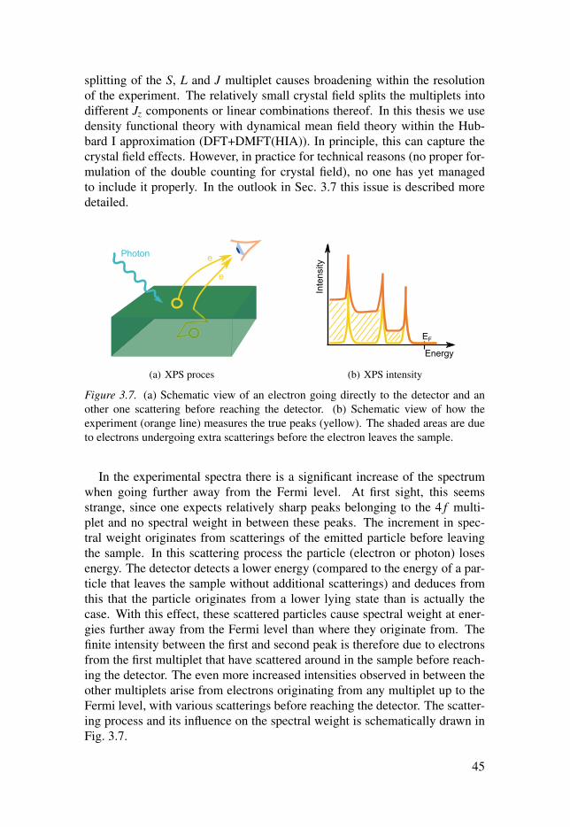
splitting of the S, L and J multiplet causes broadening within the resolution

of the experiment. The relatively small crystal field splits the multiplets into

different Jz components or linear combinations thereof. In this thesis we use

density functional theory with dynamical mean field theory within the Hub-

bard I approximation (DFT+DMFT(HIA)). In principle, this can capture the

crystal field effects. However, in practice for technical reasons (no proper for-

mulation of the double counting for crystal field), no one has yet managed

to include it properly. In the outlook in Sec. 3.7 this issue is described more

detailed.

(a) XPS proces (b) XPS intensity

Figure 3.7. (a) Schematic view of an electron going directly to the detector and an

other one scattering before reaching the detector. (b) Schematic view of how the

experiment (orange line) measures the true peaks (yellow). The shaded areas are due

to electrons undergoing extra scatterings before the electron leaves the sample.

In the experimental spectra there is a significant increase of the spectrum

when going further away from the Fermi level. At first sight, this seems

strange, since one expects relatively sharp peaks belonging to the 4 f multi-

plet and no spectral weight in between these peaks. The increment in spec-

tral weight originates from scatterings of the emitted particle before leaving

the sample. In this scattering process the particle (electron or photon) loses

energy. The detector detects a lower energy (compared to the energy of a par-

ticle that leaves the sample without additional scatterings) and deduces from

this that the particle originates from a lower lying state than is actually the

case. With this effect, these scattered particles cause spectral weight at ener-

gies further away from the Fermi level than where they originate from. The

finite intensity between the first and second peak is therefore due to electrons

from the first multiplet that have scattered around in the sample before reach-

ing the detector. The even more increased intensities observed in between the

other multiplets arise from electrons originating from any multiplet up to the

Fermi level, with various scatterings before reaching the detector. The scatter-

ing process and its influence on the spectral weight is schematically drawn in

Fig. 3.7.

45

3.5.3 Multiplet structure

With the photoemission experiments one measures transitions from the Hund’s

rule ground state with f n electrons and quantum numbers L, S and J to the

excited state with f n−1 electrons and quantum numbers L′, S′ and J′. The

inverse photoemission experiments probe f n → f n+1 transitions. Which of

the final states are accessible from the Hund’s rule ground state depends on

the selection rules [5]. For XPS, where one electron is removed, S− S′ = 12 .

The maximal amount of angular momentum which can leave the system is

±l, where l is the angular momentum quantum number of the shell where the

electron is removed from. Therefore |L−L′| ≤ l.As an illustrative example, we consider the XPS spectrum of Nd that probes

f 3 → f 2 transitions. The Hund’s rule ground state is denoted with the term

symbol 4I92. The possible final states can be found by determining all possible

ways to arrange 2 electrons over the −3≤ ml ≤ 3 and ms =±12 orbitals. This

is done in App. A and leads to the following multiplets: 1I6, 3H4,5,6, 1G4,1S0, 3F2,3,4, 1D2 and 3P0,1,2. From these multiplets only 3H4,5,6 and 3F2,3,4 are

compatible with the selection rules and can be found in the XPS spectrum.

These states will be slightly split by crystal field effects, but the separation of

the multiplet states is dominant [57].

A similar approach can be done for the BIS spectra, considering that adding

one electron is the same as removing one hole. The relative intensity of these

different multiplets can be calculated from the coefficients of fractional parent-

age, which is explained in Ref. [5] for XPS and Ref. [22] for BIS. The coef-

ficients of fractional parentage are tabulated in Ref. [5] for XPS and Chapter

62, Table I of Ref. [40] for BIS. In our work the spectra are directly calculated

from the imaginary part of the Green’s function in the DFT+DMFT(HIA) ap-

proach.

3.6 Summary of Papers I and II

Paper I: Standard model of the rare earths, analyzed from the Hubbard IapproximationIn the previous sections on the physical background of the various properties,

I tried to give an intuitive view why the standard model of the lanthanides,

that assumes a chemically inert 4 f shell, works so well. Several attempts

to apply ab-initio electronic structure calculations for real material-dependent

properties of the REs, had variable success. The typical parameterizations

of the exchange-correlation potential of DFT are inadequate to describe the

localized 4 f electrons. Theories like LDA+U [4], self-interaction correction

(SIC) [81], orbital polarization [30] and the 4 f -in-the-core approach [88] have

been tested on selected properties, and sometimes with great success. How-

ever, these methods are not able to describe a wide range of properties within

46

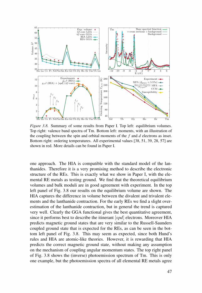
25

30

35

40

45

50

55

60

65

Ba La Ce Pr NdPmSm Eu Gd Tb Dy Ho Er TmYb Lu

VolumeA

3

-12 -10 -8 -6 -4 -2 0 2 4 6

Intensity

E (eV)

Tm

0

2

4

6

8

10

12

Ba La Ce Pr NdPmSm Eu Gd Tb Dy Ho Er TmYb Lu

mto

t Lf

Sf

SdLf

Sf

Sd

40

80

120

160

200

240

280

Gd Tb Dy Ho Er Tm

Ord

eringTem

peratu

reTN/C

(K)

Exp. volume4f -core LDA4f -core GGA

HIA LDAHIA GGA

Bare spectral function× cross sections +background

Background

ExperimentsgJJ (HIA)

gJJ (HIA) + [spd] (4f -core)

Experiment

MFA (dmax = 5.57a)(gJ−1)2J(J+1)

(Sfspd)2 MFA

CCM

Susceptibility

Figure 3.8. Summary of some results from Paper I. Top left: equilibrium volumes.

Top right: valence band spectra of Tm. Bottom left: moments, with an illustration of

the coupling between the spin and orbital moments of the f and d electrons as inset.

Bottom right: ordering temperatures. All experimental values [38, 51, 39, 28, 57] are

shown in red. More details can be found in Paper I.

one approach. The HIA is compatible with the standard model of the lan-

thanides. Therefore it is a very promising method to describe the electronic

structure of the REs. This is exactly what we show in Paper I, with the ele-

mental RE metals as testing ground. We find that the theoretical equilibrium

volumes and bulk moduli are in good agreement with experiment. In the top

left panel of Fig. 3.8 our results on the equilibrium volume are shown. The

HIA captures the difference in volume between the divalent and trivalent ele-

ments and the lanthanide contraction. For the early REs we find a slight over-

estimation of the lanthanide contraction, but in general the trend is captured

very well. Clearly the GGA functional gives the best quantitative agreement,

since it performs best to describe the itinerant [spd] electrons. Moreover HIA

predicts magnetic ground states that are very similar to the Russell-Saunders

coupled ground state that is expected for the REs, as can be seen in the bot-

tom left panel of Fig. 3.8. This may seem as expected, since both Hund’s

rules and HIA are atomic-like theories. However, it is rewarding that HIA

predicts the correct magnetic ground state, without making any assumption

on the mechanism of coupling angular momentum states. The top right panel

of Fig. 3.8 shows the (inverse) photoemission spectrum of Tm. This is only

one example, but the photoemission spectra of all elemental RE metals agree

47

very well with measured data. All multiplet features are captured and only a

small discrepancy is found in their energy positions. Additionally we use the

4 f -in-the-core approach to calculate the interatomic exchange parameters of

an effective spin Hamiltonian. We use these exchange parameters to calculate

the ordering temperatures for the heavy REs, as displayed in the bottom right

panel of Fig. 3.8. The calculated ordering temperatures agree within 20% with

measured data and capture the trent of decreasing ordering temperature across

the series. Additionally, the magnon dispersion of Gd can be used to show

the accuracy of the calculated exchange parameters. We think that the HIA

is, among the available state-of-the-art methods, the most promising one to

investigate the elemental REs or RE containing materials.

Paper II: Stacking fault energetics of α- and γ-cerium investigated with abinitio calculations

Figure 3.9. Phase diagram of Ce, data

taken from Paper II.

Cerium has a very interesting phase

diagram, see Fig. 3.9. At zero

pressure and low temperature, Ce

forms a low-volume fcc structure

(α-phase). With increasing tem-

perature a transition to the β -phase

which has a dhcp structure, occurs.

This dhcp region is rather small, and

around room temperature Ce under-

goes a new transition to the high-

volume fcc structure (γ-phase). With

moderately increased pressure the

dhcp phase disappears, and the low-

volume α-phase changes directly to

the high volume γ-phase with in-

creasing temperature [99]. Cycling

between the α and γ phase shows a hysteresis effect, where the γ → α transi-

tion occurs at a slightly lower temperature or slightly higher pressure than the

α → γ transition [100]. In Ref. [73] the authors argue that repeated cycling

would lead to dislocations. Several mechanical properties, such as hardening,

plasticity and deformations have been related to stacking fault energies, i.e.the energy needed to introduce a wrong stacking in the order of the layers.

This, together with the fact that fcc and dhcp structures are actually very sim-

ilar except for a stacking fault (see Fig. 3.3), motivates a thorough study of

stacking fault energies in Ce.

In Paper II we study the energy required for an intrinsic stacking fault, i.e. a

missing layer in the perfect fcc stacking, using both the supercell approach and

the axial interaction model. In the axial interaction model, the stacking fault

energy is related to the energies of the different possible stacking orders. We

find that the stacking fault energy for the γ-phase is much smaller than for the

48

α phase, which largely explains the hysteresis effect when cycling between

the two phases. Due to the low stacking fault energy for the γ phase, it is

very easy to introduce dislocations when going from γ → α . However, when

returning from α → γ , it is hard to introduce dislocations and therefore the

transition is delayed.

In this work the core of the calculations were done with plain DFT, since it

is computationally less demanding than the DFT+DMFT approaches that are

usually employed for Ce. The α phase was simulated with 4 f electrons as

part of the valence, which results in itinerant 4 f electrons and a small equi-

librium volume. The γ phase was simulated with the 4 f electrons as part of

the non-hybridizing core, which prevents the 4 f electrons from contributing

to the bonding and results in a bigger volume. The success of the Hubbard I

approximation for describing the γ phase of Ce, as tested in Paper I, was used

to confirm selected 4 f -in-the-core results. Both methods show very similar

stacking fault energies across the different volumes. DFT+DMFT with the

spin-polarized T-matrix fluctuation exchange (SPTF) solver was used to val-

idate the DFT calculations for the α phase. Here as well, the stacking fault

energies with both approaches were very similar.

In Paper II we model the two phases separately with two different meth-

ods. Note that in this way one can not model the phase transition itself. The

two separate stacking fault energy curves as a function of volume for the two

phases do not represent the reality in the region where the two phases coex-

ists. However, to model the stacking fault energies for the two phases sep-

arately gives theoretical insight, since this allows to describe the hysteresis

effects. DFT+DMFT with a quantum Monte-Carlo (QMC) solver could be

used to model the phase transition itself and would give a unified curve for

both phases.

3.7 Outlook

For both projects mentioned above, it would be interesting to address the co-

hesive properties in the magnetically ordered phases. The elemental REs have

an interesting magnetic phase diagram and the magnetic properties might in-

fluence the bonding properties. As mentioned in Paper I and above, both the

bonding properties and the stacking fault energies are rather sensitive quanti-

ties and mainly determined by the [spd] electrons. In DFT+DMFT a correct

description of the [spd] electrons requires a charge self-consistent calculation.

However, for charge self-consistent magnetic DFT+DMFT calculations, the

issue of the double counting, which was briefly mentioned in Sec. 2.3.5, be-

comes a problem. When combining spin-polarized DFT with DMFT the dou-

ble counting term should correct for the f - f exchange that is taken into ac-

count in both the DFT part and in U . However, it should not correct for the

f -d exchange, since this is not accounted for by U . The problem is that one

49

cannot disentangle the two, and therefore any choice becomes an unjustified

guess. This issue of the spin-polarized double counting needs to be addressed

and methodological advances for magnetic calculations are needed. This also

holds for other quantities related to magnetism such as the magnetic anisotropy

energy and related quantities. These quantities depend on a subtle balance be-

tween the crystal field effects and the spin-orbit coupling. A thorough study

is needed to investigate to what extend crystal field effects in the REs are cor-

rectly described with the HIA.

For the phase transition in Ce, related to Paper II it would be interesting

to use methods that can describe both the α and the γ phase. For this the

approximate HIA solver in the DFT+DMFT cycle is not sufficient and more

sophisticated (and costly) solvers such as the quantum Monte Carlo solver are

needed. However, a very accurate calculation of the total energy is required

for a proper assessment of the small energy differences between the different

structures.

50

4. Microscopic configuration after ultrafastmagnetization dynamics

One of the principal objects of theoretical research is to find the point of viewfrom which the subject appears in the greatest simplicity.

— Josiah Willard Gibbs (1994)

THIS chapter of my thesis is related to the field of ultrafast magneti-

zation dynamics. The kickoff of this field was given by Beaurepaire

et al. [12] in 1996 by probing for the first time the magnetization

dynamics in Ni on the femtosecond time scale. The pump-probe

experiments revealed a new type of dynamics: an ultrafast decrease of mag-

netization following a laser pulse. The experimental results were described by

modeling the material through three interacting reservoirs, belonging to the

electron system, the spin system and the lattice system. This phenomenolog-

ical model is referred to as the three temperature model. Since this first dis-

covery of ultrafast demagnetization, several other experiments have followed

and supported the findings of Beaurepaire et al. [12]. The field of ultrafast

magnetization dynamics was further investigated in various systems and new

insights were obtained. Some examples are the experimental observation of

spin transport during ultrafast magnetization dynamics in [Co-Pt]n multilay-

ers [63], the spin injection from Fe to Au on the femtosecond timescale [68]

and the discovery of ultrafast magnetization increase in Fe in a Ni/Ru/Fe tri-

layer [86].

During all these years of research, a leading question has been: what is the

underlying mechanism behind the ultrafast magnetization dynamics? In par-

ticular, where does the angular momentum related to the electron spins go?

In Fe, Ni and Co, the most commonly used materials in magnetization dy-

namics experiments, the orbital moment is quenched and the magnetization is

mainly attributed to the electron spins. Several possible mechanisms for ul-

trafast demagnetization have been proposed over the last years and they are

nicely summarized in Ref. [49]. All mechanisms consider in one way or the

other an angular-momentum transfer from the electron spins to somewhere

else. A direct contribution of the photon angular momentum in the polarized

laser beam on the demagnetization was found to be very small by experiments

in 2007 [23]. On the other hand it is of significant importance in, for ex-

ample, the inverse Faraday effect. Another possibility to carry away angular

momentum is given by the photons that are emitted during the ultrafast de-

magnetization. However it is generally believed that this effect is very small.

51

Koopmans et al. [55] suggested a model of demagnetization driven by spin-

phonon coupling, where the energy of the demagnetization comes from the

electrons, but the dissipative channel for the angular momentum is given by

the lattice. Spin-flips occur due to electron-phonon scattering. Note that this

mechanism relies on spin-orbit coupling. Another option to decrease the total

magnetization is given by transferring spin angular momentum to orbital an-

gular momentum through electron-electron scattering. The decrease of mag-

netization is then achieved, since the moment associated to the spin angular

momentum contains the gyromagnetic ratio g≈ 2. The transfer of spin to or-

bital angular momentum could also happen via electron-magnon scattering.

Battiato et al. [9] suggested that the ultrafast demagnetization and also the ul-

trafast increase of magnetization [86] are driven by superdiffusive transport

of spin. In this model the change of magnetization arrises from the differ-

ence in the mobility (velocity and lifetime) of the majority and minority spin

electrons that are excited by the laser pulse. This difference causes a net spin

transport. The model of superdiffusive spin transport was developed for met-

als, such as Ni and Fe, but later extended to semiconductors [10]. Many of the

above mentioned mechanisms are theoretically possible, but the question is to

what extent they contribute to the demagnetization process. This depends on

the specific case, the material and the geometry of the sample. It is becoming

more common to think of a coexistence of effects [95, 93].

The above mentioned experiments were done on transition metals, where

the magnetism arises from the d electrons. However, ultrafast magnetization

decrease has also been measured in Gd [19]. As mentioned in Chapter 3, the

magnetism in the REs arises from the localized 4 f electrons. This moment

exchange-couples to itinerant [6s6p5d] valence electrons inducing a moment

of about 0.6μB. The fact that the magnetism arises from two very different

types of electrons that only weakly interact adds complexity to how to describe

the magnetization dynamics.

However, even without this extra complexity, it is already very difficult to

find a good correspondence between theory and experiment. The field of ultra-

fast magnetization dynamics deals with strongly out-of-equilibrium situations.

Theoretically we can not treat this very complex out-of-equilibrium physics

directly and assumptions and simplifications have to be made. In order not to

over simplify the physics, but still be able to establish a connection between

fundamental microscopic quantities and experimentally observed quantities,

we move to the picosecond time scale in Paper III. This is the timescale when

the ultrafast magnetization dynamics process has ended1. We show that in

this time scale a partial thermal equilibrium is reached in which we can con-

nect theory and experiment. In the following I will present shortly the idea

1The exact times scales depend on several factors such as the material under investigation. For

simplicity we stick to the nomenclature of Paper III and name the sub picosecond time scale the

time during which the ultrafast magnetization dynamics take place. With the picosecond time

scale we intend the time after the ultrafast process.

52

of the work we have done in Paper III. This paper involves many different

fields of physics, arguments, and inferences, which makes it quite compli-

cated to follow the main idea. I therefore have chosen to give an overview

of this paper to illustrate the fundamental line of thoughts. As a result this

chapter is structured in a slightly different way than the previous chapter and

starts with a summary of Paper III. After that I will give some more details

on the magneto-optical effects that are used as experimental evidence for ul-

trafast magnetization dynamics. In the end I will present some preliminary

results related to the commonly used assumption that the magnetic asymmetry

measured in experiments is proportional to the magnetization.

4.1 Summary of Paper III: Microscopic configurationafter ultrafast magnetization dynamics

Although the underlying mechanism of the ultrafast magnetization dynamics

is an extremely interesting topic, it has been difficult to make a connection be-

tween measured quantities and microscopic properties. Therefore in Paper III,

we try to fill this gap by focussing on the microscopic electronic state directly

after the ultrafast process. As mentioned above, this is needed to avoid the

strong out-of-equilibrium situation during the process itself. After the ultra-

fast dynamics, the system attains a partial thermal equilibrium, which we can

address with known theoretical tools. This enables us to make a connection

between theory and experiment. The work in Paper III was inspired by various

experiments on ultrafast magnetization dynamics and in particular by the ex-

periments in Refs. [86, 93] on Fe and Ni. In these works the authors show that

ferromagnetic Fe can undergo both an ultrafast decrease and increase of mag-

netization (Fig. 4.1(a)). These processes result in two qualitatively different

experimentally observed transverse magneto-optical Kerr effect (T-MOKE)

spectra at the 3p absorption edge of Fe (Fig. 4.1(d)). We were wondering

whether this difference in the T-MOKE spectra, could be explained from the

magnetic state just after the ultrafast process. In Paper III we propose a model

to predict the microscopic electronic and magnetic configuration after ultrafast

magnetization dynamics and we indeed support the difference in the T-MOKE

spectra.

The main question of this work is: What is the magnetic configuration af-

ter ultrafast increased magnetization or after an ultrafast demagnetization on

a microscopic level? To address this question, we identify and classify all

possible microscopic states. The first step is to consider that in the picosec-

ond time scale one can already describe the system with well defined atomic

magnetic moments [6]. Examples of microstates classified with respect to

their magnetic moments are reported in Fig. 4.1(b), for both the magnetized

and demagnetized cases. Note that we only show here the magnetic part of the

configuration, as illustrated by the atomic magnetic moments, and not the elec-

53

Figure 4.1. Illustration of the main idea of the work in Paper III. (a). The experiments

showing the ultrafast increase (red) and decrease (blue) of the T-MOKE area in Fe

as reported in Ref. [93]. This T-MOKE area is related to the magnetization. (b).

Our identification of the microscopic states after the ultrafast dynamics. (c). The

off-diagonal components of the dielectric tensor for the proposed configurations for

several magnetizations Mtot. (d). The T-MOKE spectrum after an ultrafast increase of

magnetization as reported in Ref. [93] (top, red) and a sketch of the T-MOKE after an

ultrafast decrease of magnetization (bottom, blue), compared to the T-MOKE before

the laser excitation (yellow).

tronic part. For the demagnetized case (blue line in panel (a)), one can imagine

that the magnitude of the atomic spins would decrease, as illustrated by the

blue arrows in panel (b). Another option would be that the atomic moments

retain their length, but tilt in various directions, which effectively decreases

the total magnetization (illustrated by the yellow tilted arrows). Obviously, in-

termediate states are also possible. Similarly for increased magnetization, one

could imagine that the magnitude of the individual atomic magnetic moments

increases (illustrated by the straight red arrows in panel (b)). In case of tilted

moments, this increase must be even larger (illustrated by the tilted dark red

arrows in panel (b)).

In our model we integrate out the electronic degrees of freedom, which al-

lows us to identify the configurations in the green boxes (Fig. 4.1(b)) as the

most probable ones. For the demagnetized case, we predict that the atomic

magnetic moments retain their lengths, but magnon excitations cause a de-

crease of the total magnetic moment. In the case of increased magnetization

instead, we predict an increase of the magnitude of the individual atomic mag-

netic moments. These predictions are obtained through statistical arguments,

which are presented in Paper III and are summarized at the end of this para-

graph.

Starting from the magnetic configurations, we can calculate the dielectric

tensor. The T-MOKE spectrum measured in the experiments is proportional

to the off-diagonal element of the dielectric tensor, if this element is small.

Both these quantities are illustrated in Fig. 4.1(c) and (d). For the increased

magnetization case, denoted by the red lines compared to yellow (equilibrium)

54

lines in Fig. 4.1(c) and (d), we see that a shoulder develops just below the main

peak. The main peak itself retains its height. We recognize the same behavior

both in the off-diagonal element of the dielectric tensor, as well as in the T-

MOKE spectrum. A quite different behavior is seen for the demagnetized case,

where the main peak in the off-diagonal component of the dielectric tensor

decreases proportionally to the magnetic moment. Also the height of main

peak in the experimentally measured asymmetry decreases with decreasing

moment.

In Paper III one can find all details on the foundation of our model leading

to the predicted configurations. Since many different arguments and corollar-

ies come together in a complex way, I tried to outline them in the scheme in

Fig. 4.2. We describe how we characterize different time scales (illustrated

in panel (a) of Fig. 4.1), and how this allows us to consider a partial ther-

mal equilibrium just after the ultrafast magnetization dynamics. The “partial”

attribute refers to the system having a magnetization that is either bigger or

Figure 4.2. Outline of arguments, corollaries, assumptions and intermediate results of

Paper III. These apply to 3d electrons in Fe and Ni, but are likely to be generalized to

other systems as well.

55

smaller than the equilibrium magnetization. This partial equilibrium allows

us to use statistical arguments to predict the microscopic configuration. The

adiabatic approximation [6] allows us to separate the magnetic and electronic

degrees of freedom and to define the microstates by their magnetic and elec-

tronic configuration. For each total energy and total magnetic moment, we

group the microstates according to the magnetic configuration, i.e., the length

and orientation of the atomic magnetic moments. These groups of microstates

with the same magnetic configuration, but different electronic configurations,

we call mesostates. Then we compute the number of microstates within one

mesostate to identify the most probable mesostate. It turns out that the number

of microstates depends on the energy of the given magnetic configuration of

the mesostate for the lowest possible electronic configuration. Hence, we cal-

culate the energy of the magnetic configuration of the mesostates and identify

the most probable mesostate for each scenario. As mentioned above, this re-

sults in collinear atomic magnetic moments with increased magnitude for the

case with increased magnetization, and in gradually tilted atomic magnetic

moments with equilibrium magnitude after ultrafast demagnetization. The

model that we propose determines the magnetic configuration just after the

ultrafast magnetization dynamics, and makes it possible to compare the mea-

sured data to results that are calculated from microscopic properties. Hence

we can calculate the dielectric response around the 3p absorption edge of Fe

for the predicted configurations and compare this to the experimentally mea-

sured asymmetry in the T-MOKE spectra. As is shown in panel (d) of Fig. 4.1,

the T-MOKE spectrum of the increased magnetization case is qualitatively dif-

ferent from the decreased magnetization case. The dielectric tensor, calculated

from the states predicted in our model, shows exactly the same qualitative dif-

ference, as is shown in panel (c) of Fig. 4.1. Hence our model can explain the

qualitatively different behavior in the two cases.

In the next section we will briefly discuss the different MOKE experiments

and the experimental setup as used in for example Refs. [86, 93, 56]. There-

after, we will discuss the dielectric tensor and its relation to the MOKE prop-

erties briefly, because it is here where theory and experiment meet each other.

4.2 Magneto-optics

Magneto-optical effects were first discovered in the 19th century when Fara-

day found that the polarization vector of linearly polarized light rotates when

the light travels through a sample with a magnetization parallel to the propaga-

tion direction of the light [31]. Since this discovery also other magneto optical

effects where discovered, such as the Kerr effect. In this thesis we discuss

the magneto-optical Kerr effect (MOKE), which describes how light changes

upon reflecting from a magnetic surface. The review of H. Ebert [29] has been

very helpful for this section.

56

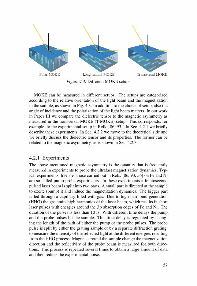
Figure 4.3. Different MOKE setups

MOKE can be measured in different setups. The setups are categorized

according to the relative orientation of the light beam and the magnetization

in the sample, as shown in Fig. 4.3. In addition to the choice of setup, also the

angle of incidence and the polarization of the light beam matters. In our work

in Paper III we compare the dielectric tensor to the magnetic asymmetry as

measured in the transversal MOKE (T-MOKE) setup. This corresponds, for

example, to the experimental setup in Refs. [86, 93]. In Sec. 4.2.1 we briefly

describe these experiments. In Sec. 4.2.2 we move to the theoretical side and

we briefly discuss the dielectric tensor and its properties. The former can be

related to the magnetic asymmetry, as is shown in Sec. 4.2.3.

4.2.1 Experiments

The above mentioned magnetic asymmetry is the quantity that is frequently

measured in experiments to probe the ultrafast magnetization dynamics. Typ-

ical experiments, like e.g. those carried out in Refs. [86, 93, 56] on Fe and Ni

are so-called pump-probe experiments. In these experiments a femtosecond

pulsed laser beam is split into two parts. A small part is directed at the sample

to excite (pump) it and induce the magnetization dynamics. The bigger part

is led through a capillary filled with gas. Due to high harmonic generation

(HHG) the gas emits high harmonics of the laser beam, which results in short

laser pulses with energies around the 3p absorption edges of Fe and Ni. The

duration of the pulses is less than 10 fs. With different time delays the pump

and the probe pulses hit the sample. This time delay is regulated by chang-

ing the length of the path of either the pump or the probe pulses. The probe

pulse is split by either the grating sample or by a separate diffraction grating,

to measure the intensity of the reflected light at the different energies resulting

from the HHG process. Magnets around the sample change the magnetization

direction and the reflectivity of the probe beam is measured for both direc-

tions. This process is repeated several times to obtain a large amount of data

and then reduce the experimental noise.

57

4.2.2 Dielectric tensor

The interaction between light (electromagnetic radiation) and a crystal can be

described by the dielectric tensor (or the related electric susceptibility) that

relates the electric field and the polarization field in Maxwell’s equations. The

magneto-optical properties can therefore be derived from the energy depen-

dent dielectric tensor ε(E). The form of this tensor is dictated by the sym-

metry of the system, which depends, amongst others, on the magnetization

direction. For a cubic system, with a finite magnetization in the z-direction,

only five components of the dielectric tensor have a finite value. The xx and yy-

component are the same, for symmetry reasons. The zz-component is slightly

different, since the magnetic moment is in the z-direction. Only two of the

off-diagonal components are non-zero. This results in a dielectric tensor of

the following form

ε(E) =

⎛⎝ εxx(E) εxy(E) 0

−εxy(E) εxx(E) 0

0 0 εzz(E)

⎞⎠ , (4.1)

where εxy(E) changes sign upon reversing the direction of the magnetic field.

Note also that the change in symmetry due to magnetization, only happens

due to the spin-orbit coupling. Therefore spin-orbit coupling is crucial for the

magneto-optical effects.

The dielectric tensor can be obtained from band-structure calculations in

combination with linear response theory using the Kubo formalism [83]. This

formalism relates the dielectric tensor to transitions from occupied to unoccu-

pied states. To get a feeling of how the dielectric tensor looks like, we show

the density of states and some parts of the dielectric tensor for Fe in Fig. 4.4.

In this thesis we are interested in the magneto optical effects around the 3p ab-

sorption edge of Fe and Ni. We therefore consider, as an example, Fe around

this energy, i.e. the interval 50-60 eV. The upper row displays the density

of states and several parts of the dielectric tensor in case no magnetization is

present. The bottom row displays the same quantities for equilibrium mag-

netization in Fe along the z-direction. For zero magnetization, the diagonal

components of the dielectric tensor have a finite value and are all the same,

see top middle panel of Fig. 4.4. The spin-dependent off-diagonal compo-

nents also have a finite value, but the majority and minority spins cancel each

other, see top rightmost panel of Fig. 4.4. This gives, for zero magnetization,

a purely diagonal dielectric tensor. It is interesting to compare the density of

states (leftmost panels in Fig. 4.4) to the dielectric tensor (rightmost panels in

Fig. 4.4) for this case. For zero magnetization, the two peaks in the density

of states due to the core levels are well defined and clearly separated. This

means that the dielectric tensor for this case bears a strong resemblance with

the density of states just above the Fermi level. One can see that the dielectric

58

Figure 4.4. Density of states (left) and dielectric tensor (middle and right) of Fe. Top

figures are for zero magnetization, bottom figures for equilibrium magnetization.

tensor probes somehow transitions from the 3p core level to the unoccupied

states in the valence.

For a finite magnetization in the z-direction, the zz-component is different

from the xx-component. For the off-diagonal elements, majority (down) and

minority (up) spins do not cancel anymore. One can see that transitions for

the majority spin electrons are less probable than those for the minority spin

electrons, since, just above the Fermi level, the density of states of the majority

spin electrons is much smaller than that of the minority spin electrons, see

bottom panels of Fig. 4.4.

The dielectric tensor can be used to calculate the magneto-optical effects.

In the next section we focus on the magnetic asymmetry in the T-MOKE setup,

since we compare our theoretical results of the dielectric tensor to the magnetic

asymmetry measured in ultrafast magnetization dynamics experiments [86,

93].

4.2.3 Relation asymmetry and dielectric tensor

The propagation of light in a medium is described by the Maxwell equations

together with some material relationships that relate the displacement field Dand the magnetizing field H to the electric field E and the magnetic field Brespectively, and Ohm’s law [18]. In our case it is sufficient to use the material

dependent dielectric tensor that relates the electric displacement to the electric

field. Or equivalently the conductivity tensor that relates the current density to

the electric field [18]. The Maxwell equations, the material relationships and

Ohm’s law can be combined into the Fresnel equations [18]. With the latter

and the boundary conditions, i.e. the continuity requirements for the Maxwell

equations, the MOKE spectra can be calculated. We are especially interested

in the magnetic asymmetry in the T-MOKE setup. This is given by the dif-

59

ference between the reflection of the (p polarized) beam from a sample with

the magnetization in the z-direction (R+) and in the −z-direction (R−), nor-

malized by the sum. For a single element layer and for a small off-diagonal

component εxy(E) of the dielectric tensor, the magnetic asymmetry is propor-

tional to εxy(E) itself [18, 65]:

A(E) =R+(E)−R−(E)R+(E)+R−(E)

≈ Re

(2ε0εxy(E)sin(2φ)

εxx(E)2 cos2(φ)− ε0εxx(E)+ ε20 sin2(φ)

), (4.2)

where ε0 is the vacuum dielectric permittivity and φ the angle of incidence

of the beam. For small moments, and hence small εxy(E), the asymmetry is

proportional to both the real and imaginary part of εxy(E). Various works addi-

tionally assume that εxy(E) is proportional to the magnetization [65] and hence

that the magnetic asymmetry is proportional to the magnetization. Or at least

that the magnetic asymmetry increases when the magnetic moment increases.

Therefore, they use the magnetic asymmetry to probe the magnetization of

the sample. Instead of using the approximate solution in Eq. 4.2, the Fresnel

equations can also be solved numerically [94, 98]. With this procedure one

could check the validity of the approximations made for the above equation.

This issue will be analyzed in more detail in the next section.

4.3 Is the magnetic asymmetry proportional to thesample magnetization?

In Paper III we predicted the microscopic state after the ultrafast magnetiza-

tion dynamics has taken place. We managed to qualitatively explain the differ-

ence between the T-MOKE spectrum after ultrafast demagnetization and the

spectrum after increase of magnetization. The development of the shoulder at

lower energies in the latter case is explained by our model, as well as the shape

conserving decrease of the peak in the former case. In this section I would like

to focus on some preliminary results on the quantitative relation between the

magnetic asymmetry and the magnetization of the sample. We investigate the

proportionality often assumed in experiments: A(E) ∝ M. This ongoing work

is in collaboration with the Molecular and Condensed Matter Physics group in

Uppsala and a preliminary draft is given in Paper IV.

4.3.1 Before the laser pulse: equilibrium situation

Before turning our attention to the relation between the magnetic asymmetry

and the magnetization, we investigate the correspondence between the the-

oretically calculated magnetic asymmetry and the experimentally measured

60

one. The dielectric tensor for the equilibrium state can be obtained using DFT

calculations as mentioned in Sec. 4.2.2. From this dielectric tensor we can

numerically solve the Fresnel equations [94, 98] to obtain the magnetic asym-

metry for a specific geometry. Before comparing the theoretically calculated

magnetic asymmetry to the experimental asymmetry, let us emphasize that the

theoretical calculations are strongly simplified with respect to the range of ef-

fects affecting a complex experiment. The effect of these simplifications is

not yet clear, but it would be very interesting to investigate it. Examples of

discrepancies between theory and experiment are

Bulk versus finite slab: The dielectric tensor is calculated for bulk material.

This means that the finite size of the slab enters only through the Fresnel

equations. Reconstruction near the surface or any surface roughness are

not taken into account. Neither is the change in the electronic structure

of surface states compared to bulk states taken into account.

Impurities: Impurities that might be present in the sample are not taken into

account in theory.

Core hole effects: We calculate the dielectric tensor with the Kubo formula,

that is based on excitations from occupied (3p levels) to unoccupied (va-

lence band) states. We neglect in this case the presence of a “core-hole”

that is left around the 3p levels after the excitation. The main effect of

taking into account a core-hole is probably a shift along the energy axis

to deeper energies of the dielectric tensor. This shift is material and level

dependent.

Strain in the sample: Since the samples are usually quite thin and are grown

on some substrate, strain may occur and the lattice parameter may vary

across the layer.

Substrate and capping layer: The optical properties of the substrate on which

the sample is grown or the capping layer of the sample are not taken into

account.

Born-Oppenheimer approximation: In the DFT calculations the nuclei are

treated as fixed. Electron-phonon coupling is therefore not taken into

account. We expect the influence of lattice vibrations in Fe or Ni to be

small and mainly a tiny broadening of the spectrum.

Correlation effects: The DFT treatment of Fe and Ni is for some quantities

not adequate. The 3d bandwidth and the spin splitting are slightly over-

estimated by LDA/GGA.

Despite all these simplifications, the theoretical asymmetry for a 100nm slab

of Ni is found to agree qualitatively well with the experimental asymmetry, see

Fig. 4.5. For low energies, the experimental asymmetry is found to be negative

and becomes more negative towards the absorption edge. In the absorption

edge the asymmetry is positive and after the edge it is close to zero. We find

these features also in theory. We found only two quantitative differences. The

first one is a shift of the features towards lower energies, which can most

probably be explained by the effect of the core hole. The second disagreement

61

-0.2-0.1

00.10.20.30.40.50.6

50 55 60 65 70 75

A=

R+−R−

R++R−+δ

E(eV)

-0.2

0

0.2

0.4

0.6

0.8

50 55 60 65 70 75

A=

R+−R−

R++R−+δ

E(eV)

Experiment

Theory

Figure 4.5. Magnetic asymmetry Ni (100 nm). Upper panel: asymmetry measured

with T-MOKE on 100 nm Ni as described in Sec. 4.2.1. The grey lines denote the

energy positions of the high harmonics and the green dots denote therefore the values

of the asymmetry. Lower panel: asymmetry calculated by solving the Fresnel equa-

tions for a 100 nm layer of Ni with an ab initio calculated bulk dielectric tensor. Note

that, in the upper panel only the green dots are relevant when comparing experiment

to theory.

is that the theoretical asymmetry is found to be about 1.5 times larger than the

experimentally measured one (the y-axes in Fig. 4.5 differ by a factor 1.5).

4.3.2 After the laser pulse: recovering the equilibriummagnetization

To investigate the relation between the asymmetry and the magnetization, we

focus on the process of recovery of the magnetization after the ultrafast demag-

netization. We focus on this process and not on the process of ultrafast demag-

netization itself, since the latter is governed by strongly out-of-equilibrium

physics and too complicated to describe for now. Moreover, in Paper III we

already investigated the microscopic state of the material just after the ultra-

fast magnetization dynamics has taken place, and hence we can build on those

results. During the process of recovering the equilibrium magnetization, the

system can be treated as quasistatic with a time-dependent macroscopic mag-

netization M(t) and energy E(t). This allows us to examine the relation be-

tween the asymmetry and the magnetization.

In Paper III we identified the microscopic magnetic configuration after ul-

trafast demagnetization as a state with gradually tilting moments. With this

we mean that all atomic magnetic moments are tilted from the z-axis with an

62

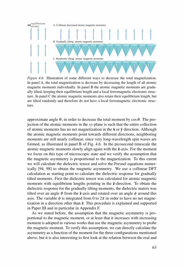
Figure 4.6. Illustration of some different ways to decrease the total magnetization.

In panel A, the total magnetization is decrease by decreasing the length of all atomic

magnetic moments individually. In panel B the atomic magnetic moments are gradu-

ally tilted, keeping their equilibrium length and a local ferromagnetic electronic struc-

ture. In panel C the atomic magnetic moments also retain their equilibrium length, but

are tilted randomly and therefore do not have a local ferromagnetic electronic struc-

ture.

approximate angle θ , in order to decrease the total moment by cosθ . The pro-

jection of the atomic moments in the xy-plane is such that the entire collection

of atomic moments has no net magnetization in the x or y direction. Although

the atomic magnetic moments point towards different directions, neighboring

moments are still nearly collinear, since very long-wavelength spin waves are

formed, as illustrated in panel B of Fig. 4.6. In the picosecond timescale the

atomic magnetic moments slowly align again with the z-axis. For the moment

we focus on this type of microscopic state and we verify the assumption that

the magnetic asymmetry is proportional to the magnetization. To this extent

we will calculate the dielectric tensor and solve the Fresnel equations numer-

ically [94, 98] to obtain the magnetic asymmetry. We use a collinear DFT

calculation as starting point to calculate the dielectric response for gradually

tilted moments. First the dielectric tensor was calculated for atomic magnetic

moments with equilibrium lengths pointing in the z-direction. To obtain the

dielectric response for the gradually tilting moments, the dielectric matrix was

tilted over an angle θ from the z-axis and rotated over an angle φ around this

axis. The variable φ is integrated from 0 to 2π in order to have no net magne-

tization in a direction other than z. This procedure is explained and supported

in Paper III and in particular in Appendix F.

As we stated before, the assumption that the magnetic asymmetry is pro-

portional to the magnetic moment, or at least that it increases with increasing

moment is adopted in various works that use the magnetic asymmetry to probe

the magnetic moment. To verify this assumption, we can directly calculate the

asymmetry as a function of the moment for the three configurations mentioned

above, but it is also interesting to first look at the relation between the real and

63

imaginary parts of εxy(E), and the magnetization. Let us start with this. For

the gradually tilting moments with varying θ this assumption is true. Indeed

Re [εxy(E)]/Re [εxy0(E)] = M/M0 and Im [εxy(E)]/Im [εxy0(E)] = M/M0 for

all energies, where the subscript 0 denotes the value at equilibrium magneti-

zation. This is actually true by construction, due to the way we calculated the

dielectric tensor for this case.

-0.15-0.1

-0.050

0.050.1

0.150.2

0.250.3

46 48 50 52 54 56 58 60

Ratio

E (eV)

0.40.5

0.60.7

0.8

0.91

0.811.21.41.61.822.2

0.40.50.60.70.80.91

A/A

0

Moment

Reduction of moment

|εxy |/|εxx|Re(εxy)/|εxx|Im(εxy)/|εxx|

(a) Fe

-0.05

0

0.05

0.1

0.15

56 58 60 62 64 66 68 70Ratio

E (eV)

0.40.5

0.60.7

0.8

0.91

0.20.30.40.50.6

0.40.50.60.70.80.91

A/A

0

Moment

Reduction of moment

|εxy |/|εxx|Re(εxy)/|εxx|Im(εxy)/|εxx|

(b) Ni

Figure 4.7. Non-linear relationship between magnetic asymmetry and magnetization

for gradually tilting moments. Top row: Ratio between off-diagonal and diagonal

components of the dielectric tensor. The grey lines denote the energies where the

asymmetry as a function of the magnetization is most non-linear. Bottom row: Rela-

tion between the asymmetry at a specific energy and the magnetization. The different

lines denote the different energies at which A/A0 is evaluated. The behavior of the

asymmetry was evaluated at all integer energies between 40-80 eV for Fe and be-

tween 50-80 eV for Ni. The dark blue line is a guide to the eye to illustrate the linear

relation A/A0 = M/M0. The most non-linear lines for Fe belong to E =54, 52, 51,

and 50 eV. The most non-linear lines for Ni belong to E =62, 61, 63, 64, 65, 60, 59,

58 and 66 eV

Secondly we can investigate the proportionality between the magnetic asym-

metry and the magnetization. We check this for all energies, by calculating

the asymmetry from the numerical solutions to the Fresnel equations. We find

that, for gradually tilting moments, where θ decreases to recover the original

magnetization, the approximate proportionality holds only for some energies,

whereas for energies in the absorption edge the asymmetry is not linearly pro-

portional to the magnetization. We show our results in Fig. 4.7. In the top

row, the ratio between the off-diagonal and diagonal components of the di-

64

electric tensor for Fe (left) and Ni (right) is shown. To obtain the asymmetry,

we solved the Fresnel equations numerically [94, 98] for a 100 nm layer of

Fe and a 100 nm layer of Ni for the scenario of gradually tilting moments.

In the bottom row of Fig. 4.7 we display the relation between the normalized

asymmetry A/A0 and the magnetic moment at several energies, calculated by

solving the Fresnel equations [94, 98]. Especially close to the absorption edge,

i.e. between 50-58 eV for Fe and between 58-68 eV for Ni, the off-diagonal

component of the dielectric tensor is not very small as can be seen in the top

row of Fig. 4.7. It is clear from our calculations that for energies in this range,

the relationship between the magnetic asymmetry and the magnetization is

non-linear.

In Paper III we identified microscopic states with gradually tilting moments

as the state just after the ultrafast magnetization dynamics has taken place

(panel B of Fig. 4.6). However, it is worth considering also a state where the

atomic magnetic moments are not gradually tilted, preserving the local ferro-

magnetic electronic structure, but are tilted randomly instead. We illustrated

this situation in panel C of Fig. 4.6. In this case the relation is expected to

be non-linear as well. For randomly titled moments, the electronic structure

is expected to change from the ferromagnetic case. This will influence the

dielectric tensor, where we expect that εxy(E) is no longer proportional to the

magnetization. This lead to the believe that the non-linearity in the asymmetry

is probably even stronger than in the case of gradually tilted atomic magnetic

moments. We are planning to investigate this scenario as well.

Finally, we would like to mention that also for the scenario with collinear

decreased atomic magnetic moments (panel A in Fig. 4.6), the relation be-

tween the asymmetry and the magnetization is not linear. We calculated the di-

electric response with a collinear constraint DFT calculation, where the atomic

magnetic moments are constraint to a value smaller than the equilibrium value.

We emphasize here that, for the collinearly decreased moments, the real and

imaginary parts of the off-diagonal component of the dielectric tensor are not

proportional to the magnetization. Around as well as in the absorption edge,

the relation between Re [εxy(E)] and the magnetic moment is strongly non-

linear. At some energies Re [εxy(E)] even increases with decreasing magneti-

zation. Similar behavior is found for Im [εxy(E)]. Also the magnetic asymme-

try is not at all linearly proportional to the magnetization.

Although we can not establish a perfect quantitative agreement between the

theoretical and experimental asymmetry, we can conclude that one should be

careful with assuming a linear relationship between the magnetic asymmetry

and the magnetization. In particular close to the absorption edge strong non-

linearities are found in the theoretical calculations. In experiment a small

difference is found in the A(t)/A0 behavior for the different harmonics, as

is shown in draft of Paper IV. If A(E) ∝ M for all energies, this would not be

possible. The non-linear relationship between A and M could explain these

65

differences. However, the non-linearity found in theory seems to be much

more pronounced than the differences found in experiment.

One could try to speculate about the relationship between the asymmetry

and the magnetization during the process of ultrafast magnetization dynamics,

i.e. in the sub picosecond timescale in the previously defined nomenclature.

However, one should be extremely careful with this. During the ultrafast mag-

netization process, i.e. before the partial thermal equilibration, one can not

use (quasi-) equilibrium physics to determine averages over the microscopic

quantities to obtain the macroscopic quantities.

4.4 Outlook

Paper III was inspired by the experimental works in Refs. [86, 93] on Fe and

Ni. In these materials the magnetism arises from the d electrons. It would be

interesting to generalize the model to more complicated cases, as for instance

Gd [19, 67]. In this case more care is required since the magnetism arises both

from the itinerant [spd] valence electrons and from the localized 4 f electrons.

The [spd] and f spins interact only weakly and the question arises if to treat

these moments always parallel, or only weakly coupled or as separate degrees

of freedom [87]. Another question is whether the partial equilibration, on

which our model is based, happens with two distinct constraints regarding

the d and f magnetic moments. The most probable magnetic configurations

are likely to be much more complicated than those proposed in Paper III for

Fe. Also both Refs. [87] and [78] emphasize the difference in the electronic

structure of the bulk and surface states in Gd. This implies that great care is

required when comparing to surface sensitive experiments.

As mentioned in Sec. 4.3 it would be very helpful if we could make a quan-

titative comparison between the theoretical and experimental magnetic asym-

metry. First of all the quantitative agreement for the equilibrium state should

be improved and understood. To this extent it would be insightful to investi-

gate the influences of the discrepancies between theory and experiment listed

on page 61. After this quantitative agreement has been accomplished one

could move on to the area of recovery of the equilibrium magnetization afterthe ultrafast magnetization dynamics and use the asymmetry to get a quanti-

tative knowledge of the magnetization. The extremely brave could proceed to

the even more uncertain territory of the ultrafast magnetization change itself

and could speculate about the relation of the magnetic asymmetry to the mag-

netization during this process. A good quantitative agreement would support

and quantify the use of the magnetic asymmetry to probe the magnetization of

the sample.

With the numerical solution to the Fresnel equations, one can also investi-

gate different geometries. One can study multilayer systems, and the influence

of the capping and separation layers. This is however not so trivial, since the

66

shift in energy of the theoretical absorption edge is material dependent. When

combining several materials, these should be aligned properly.

67

5. Analytic continuation

Nothing will work unless you do.

— Maya Angelou (1969)

IN this thesis, DFT+DMFT in the Hubbard I approximation is used and

this method was implemented to calculate the spectral function directly

on the real energy axis. However, for many other solvers of the im-

purity problem in DFT+DMFT the Green’s function is only calculated

as a function of imaginary time (τ) or imaginary frequencies, i.e. Matsubara

frequencies iωn. In order to compare to experimentally observable quantities,

the Green’s function (or a related quantity) is needed as a function of real fre-

quencies ω , and this is where the problem of analytic continuation comes into

play. One needs to continue the function known on the imaginary axis in the

complex plane, to the real axis, as illustrated in Fig. 5.1. In Sec. 5.1 we in-

troduce the problem of analytic continuation related to Green’s functions and

their corresponding spectral functions. In Sec. 5.2 we briefly describe the dif-

ferent methods that we use in our work in Papers V, VI and VII. We conclude

with a summary of these works and some questions and challenges for the

future.

5.1 Spectral functions

The quantity of interest is the spectral function A(ω) at real frequency ω .

This quantity can be measured via photoemission experiments. The spectral

function is related to the imaginary part of the single particle Green’s function

on the real axis and can be obtained from the Green’s function at the Matsubara

frequencies by

G(iωn) =∫ ∞

−∞dω

1

iωn−ωA(ω). (5.1)

The Green’s function in the above equation is a function of the fermionic

Matsubara frequencies iωn = i (2n+1)πβ , where β is the inverse temperature

and n is an integer. The Green’s function is analytic in the entire complex

plane, except on the real axis. The spectral function is proportional to the

discontinuity in the imaginary part of the Green’s function on the real axis

A(ω) =− 1π Im[G(ω + iδ+)], where δ+ indicates that we take the limit to zero

68

ω0 = (2∗0+1)πβ

ω1 = (2∗1+1)πβ

ωn = (2∗n+1)πβ

ω

Analytic continuation from

the imaginary to

the real axis

iωn

Im(G

(iωn))

ω

Im(G

(ω+iδ

+))

Figure 5.1. Schematic representation of the idea of analytic continuation

from above δ → 0+ . The Green’s function is often decomposed in a non-

interacting part and a part that contains the interactions, i.e. the self-energy,

see Sec. 2.3. Thus instead of continuing the Green’s function to the real axis,

one can also continue the self-energy.

An example of a one-particle Green’s function can be found in Sec. 2.3.2.

In Eq. 2.15, the one-particle impurity Green’s function of the single impu-

rity Anderson model is given as a function of imaginary time. The single

Anderson impurity model Hamiltonian is time independent and therefore the

Green’s function depends only on the time difference τ−τ ′. To obtain the cor-

responding spectral function A(ω) one could first Fourier transform Eq. 2.15

to Matsubara frequencies and subsequently use Eq. 5.1 to obtain the spectral

function. Alternatively one can also perform directly the analytic continuation

from imaginary time to real frequencies:

G(τ) =∫ ∞

−∞dω

e−τω

1+ e−βω A(ω). (5.2)

The previous discussion was focussed on one-particle Green’s functions, as

these are mainly considered in this thesis. In DMFT (and also in the Hubbard

I approximation) the one-particle Green’s function is a key quantity of the

method and the calculations. In Paper I we calculated the one-particle spectral

function of the elemental rare earth metals and compared it to the experimental

valence band spectra. In Papers V and VII we tested the analytic continuation

of one-particle Green’s functions. However, dynamic two-particle quantities

69

have also received more and more attention in recent years. These two-particle

Green’s functions are used to calculate the linear response of a system to a

small external perturbation. For example, a perturbation by a small electric

field gives information about the optical conductivity and by a small magnetic

field about the spin-susceptibility. In Paper VI, we therefore focussed on the

analytic continuation of two-particle quantities.

As an example, the two-particle Green’s function corresponding to the sin-

gle impurity Anderson model in Sec. 2.3.2 is:

G(τ1,τ2,τ3,τ4) =−〈Tcσ1(τ1)c†

σ2(τ2)cσ3

(τ3)c†σ4(τ4)〉. (5.3)

Since the Hamiltonian is time independent, the Green’s function actually de-

pends on time differences and in the above equation one imaginary time vari-

able can be eliminated. The four spin indices can be reduced to only two for

symmetry reasons. After Fourier transforming the two-particle Green’s func-

tion to imaginary frequencies, the three fermionic frequencies can be com-

bined into one bosonic frequency iωn = i 2nπβ and two fermionic frequencies.

For one-frequency Green’s functions (or susceptibilities), the three-frequency

Green’s function can be summed over the fermionic frequencies. The final

one-frequency Green’s function depends on a single bosonic frequency, see

Ref. [84] for a thorough introduction to n-particle Green’s functions.

Dynamical two-particle quantities have slightly different properties and sym-

metry relations, as described in Paper VI. The most important difference, com-

pared to the one-particle spectral function, is that, along the real energy axis,

the two-particle spectral function is odd, i.e. A(ω) = −A(−ω). Contrary to

the one-particle spectral function that is even, i.e. A(ω) = A(−ω). Therefore,

the asymptotic behavior for large n of the two-particle Green’s function is ω−2n

instead of the ω−1n behavior for one-particle Green’s functions.

5.2 Methods of analytic continuationThe relation between the Green’s function and the spectral function can be

rewritten as a Fredholm integral of the first kind1:

G(y) =∫

K(y,x)A(x)dx. (5.4)

Here G(y) are the known data, A(x) is the unknown model and K(y,x) is the

integral kernel that relates the model and the data. In relation to Eq. 5.1 the

1The inversion of this Fredholm integral is not only relevant for the analytic continuation of

Green’s functions, but also in completely different areas of science. Such as in the inverse

problem for electroencephalography (EEG) source localization, where the measured voltage

potential on the scalp should reveal current sources inside the brain [35], or in electrocardiogra-

phy (ECG) where on the body measured voltage potentials provide information about currents

in the heart muscle [17].

70

data are given by the Green’s function G(iωn), the model is the spectral func-

tion A(ω) and the Kernel takes the form 1iωn−ω . For the analytic continuation

from imaginary time to real frequencies, the data and the Kernel are slightly

different, as is also the case for the two-particle Green’s functions. The model

A(x) can be always written in such a form that A(x)≥ 0. For the odd bosonic

spectral function, this means for example that one obtains ωA(ω)≥ 0 and that

the Kernel is adjusted accordingly.

In the complex case, the Fredholm integral is easily separated into real and

imaginary parts, since the model A(x) is real. This means that the integral can

be split ∫[K1(y,x)+ iK2(y,x)]A(x)dx = G1(y)+ iG2(y) (5.5)

⇒{ ∫

K1(y,x)A(x)dx = G1(y)∫K2(y,x)A(x)dx = G2(y).

where the subscript 1 denotes the real part and 2 the imaginary part. Although

it looks as a simple equation, this is only apparent. Finding A given G is

an inverse problem and usually very complicated. Especially in real world

problems, where the data is known only on a finite number of points and only

with finite precision, it is generally an ill-posed problem. If there exists an

A(x) that produces the data G(y) there are usually infinitely many solutions,

and it is not clear which one to pick. Even more worrying, generally there is

no exact solution: there is no A that reproduces G. The aim of the analytic

continuation methods is finding the best possible A.

There are several quite different approaches to find A(ω) given G(iωn). The

methods that we use are illustrated in Fig. 5.2 and we will describe them in the

following of this chapter. For the general idea, it is convenient to divide the

methods into categories. One category of approaches consists in fitting a func-

tion to the known data G(iωn). In this G(z) can be obtained anywhere in the

complex plane and A(ω) is given by− 1π Im[G(ω + iδ+)] at a small distance δ

from the real axis. In the Padé approximant method of analytic continuation,

this approach is used with a fraction of polynomials as the fitting function. A

brief explanation of this approach is given in Sec 5.2.1. We thoroughly inves-

tigate the capabilities of the Padé method for fermionic Green’s functions and

self-energies in Paper V. In Paper VI we test it for two-particle Green’s func-

tions. Note that in this approach one uses the fact that A(ω) is proportional to

the imaginary part of the Green’s function, when evaluating the fitting func-

tion close to the real axis. This proportionality is not assumed in the other

methods, which are in this sense more general. That is, they are in principle

applicable to each Fredholm equation of the first kind, regardless of the kernel

or the relation between G and A.

A quite different category of approaches is based on random sampling

methods to make guesses of A(x). Eq. 5.4 is then used to obtain G(y), which

is compared to the known data set. According to an algorithm based on the

71

Figure 5.2. Illustration of the different categories of analytic continuation methods

described in this chapter, for details see text.

difference between the calculated and known G(y), the random changes in

A(x) are accepted or rejected in a Monte Carlo chain. The method of ana-

lytic continuation developed by Mishchenko et al. [70] is based on solving the

Fredholm equation in such a way. We will discuss this method in Sec. 5.2.2. In

Paper VII we implemented this method on a Graphics Processing Unit (GPU).

In Paper VI we compared this method to other methods for the analytic con-

tinuation of bosonic Green’s functions.

The last category that we will discuss includes least square minimization

methods. In these methods the problem in Eq. 5.4 is discretized and written in

a matrix from. This matrix equation gives rise to a least square minimization

problem. Because of the ill-posed nature of the inverse problem, regulariza-

tions are needed to obtain a unique solution that is not dominated by noise.

We will address regularizations used in the non-negative least square (NNLS)

approach, the non-negative Tikhonov (NNT) approach and the maximum en-

tropy method (MEM) in Sec. 5.2.3.

5.2.1 Padé approximant method

In the Padé approximant method a function G(z) is fitted to the input data

G(iωn). The analytic structure of the data is usually not known, but the Padé

method assumes that the function can be written as a fraction of two poly-

nomials P(z) and Q(z), with complex coefficients pi and qi respectively. To

obtain the correct asymptotic behavior, 1/z for one-particle Green’s functions

and 1/z2 for two-particle functions, the polynomial degree of Q(z) is respec-

tively one or two higher than the polynomial degree of P(z). For now we focus

on the fermionic case, but everything is easily extended to the bosonic case2.

2For bosonic Green’s functions the asymptotic behavior for large z is 1/z2, the fractional poly-

nomial can already have this form by assuming pr = 0.

72

The fractional polynomial can be explicitly written as:

G(z) =P(z)Q(z)

=p1 + p2z+ . . .+ przr−1

q1 +q2z+ . . .+qrzr−1 + zr . (5.6)

There are several schemes for finding the Padé approximant, such as Thiele’s

reciprocal difference method [8] or Beach’ algorithm [11]. We use the latter

approach for finding the Padé approximant. In Beach’ scheme the 2r unknown

complex coefficients, i.e. pi and qi, are calculated by specifying G(z = iωn) =G(iωn) for 2r Matsubara points. Using 2r Matsubara frequencies to calculate

2r unknown coefficients results in a set of 2r linear equations. Beach et al. [11]

conveniently casted these equations in a matrix form, by defining the column

vectors

(pq

)=

⎛⎜⎜⎜⎜⎜⎜⎜⎝

p1...

prq1...

qr

⎞⎟⎟⎟⎟⎟⎟⎟⎠∈ C2r and G =

⎛⎜⎜⎜⎝

Giω1(iω1)

r

Giω2(iω2)

r

...

Giω2r(iω2r)r

⎞⎟⎟⎟⎠ ∈ C2r. (5.7)

In the above definition we denote the datapoint at iωn with Giωn to avoid con-

fusion with multiplication by (iωn)r. With these definitions and the row vector

(1 z z2 . . . zr−1), the approximant G can be rewritten as:

G =(1 z z2 . . . zr−1) ·p

(1 z z2 . . . zr−1) ·q+ zr . (5.8)

This casts the set of 2r linear equations (Giωn = Giωn) into the following form:

⎛⎜⎜⎜⎝

1 iω1 . . . (iω1)r−1 −Giω1

. . . −Giω1(iω1)

r−1

1 iω2 . . . (iω2)r−1 −Giω2

. . . −Giω2(iω2)

r−1

......

......

...

1 iω2r . . . (iω2r)r−1 −Giω2r . . . −Giω2r(iω2r)

r−1

⎞⎟⎟⎟⎠(pq

)= G .

(5.9)

If we now denote the matrix in the above equation as K ∈ C2r×2r, the prob-

lem of finding the coefficients {pi} and {qi} boils down to an inverse matrix

problem: (pq

)= K −1G . (5.10)

Typically the condition number of this matrix is very high and it is very hard to

take a good numerical inverse. For an inverse of K that is a not dominated by

numerical errors, a fairly high numerical precision is needed. An estimate for

73

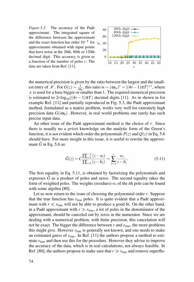
Figure 5.3. The accuracy of the Padé

approximant. The integrated square of

the difference between the approximant

and the exact function has order 10−F for

approximants obtained with input points

that have noise at the 20th, 80th or 120th

decimal digit. This accuracy is given as

a function of the number of poles r. The

data are taken from Ref. [11].

0

20

40

60

80

10 15 20 25 30 35 40 45 50

F

r

20th digit80th digit

120th digit

the numerical precision is given by the ratio between the largest and the small-

est entry of K . For G(z)∼ 1iωn

, this ratio is∼ (ω2r)r = [(4r−1)πT ]±r, where

± is used for a base bigger or smaller than 1. The required numerical precision

is estimated to 2r log10((4r− 1)πT ) decimal digits [11]. As in shown in for

example Ref. [11] and partially reproduced in Fig. 5.3, the Padé approximant

method, formulated as a matrix problem, works very well for extremely high

precision data G(iωn). However, in real world problems one rarely has such

precise input data.

An other issue of the Padé approximant method is the choice of r. Since

there is usually no a priori knowledge on the analytic form of the Green’s

function, it is not evident which order the polynomials P(z) and Q(z) in Eq. 5.6

should have. For more insight in this issue, it is useful to rewrite the approxi-

mant G in Eq. 5.6 as:

G(z) =C∏r−1

i=1 (z−ai)

∏ri=1 (z−bi)

=r

∑i=1

wi

z−bi. (5.11)

The first equality in Eq. 5.11, is obtained by factorizing the polynomials and

expresses G as a product of poles and zeros. The second equality takes the

form of weighted poles. The weights (residues) wi of the ith pole can be found

with some algebra [80].

Let us now return to the issue of choosing the polynomial order r. Suppose

that the true function has rtrue poles. It is quite evident that a Padé approxi-

mant with r� rtrue will not be able to produce a good fit. On the other hand,

in a Padé approximant with r� rtrue, a lot of poles in the denominator of the

approximant, should be canceled out by zeros in the numerator. Since we are

dealing with a numerical problem, with finite precision, this cancelation will

not be exact. The bigger the difference between r and rtrue, the more problems

this might give. However rtrue is generally not known, and one needs to make

an estimated guess of rtrue. In Ref. [11] the authors propose a method to esti-

mate rtrue and then use this for the procedure. However they advise to improve

the accuracy of the data, which is in real calculations, not always feasible. In

Ref. [80], the authors propose to make sure that r� rtrue and remove superflu-

74

ous poles from the approximant. They propose several methods to select this

spurious pole-zero pairs.

The problem of taking r� rtrue is that one fits the approximant partially to

numerical noise. This results in not exactly canceling pole-zero pairs which

gives rise to spurious features in the spectrum. In Paper V we try to tackle this

problem in two ways. First the over-fitting is reduced by considering more

input points than Padé coefficients. Second, an average is taken over several

continuations. Since one expects noise to be random, one also expects the spu-

rious features, i.e. the not exactly canceling zero-pole pairs to be distributed

randomly for different r. The average over several continuations with different

r should average out the spurious features. As to the first point, in order to have

more input points than Padé coefficients, the matrix problem should be refor-

mulated in a least-square minimization, as was already suggested in Ref. [79].

So instead of 2r Matsubara frequencies, we now consider M ≥ 2r data points

and the vector G in Eq. 5.7 becomes G ∈ CM . The matrix K in Eq. 5.9 will

have M rows, but still 2r columns, i.e. K ∈CM×2r. The coefficients are found

by least square minimization:

min‖K(pq

)−G ‖. (5.12)

Since there are “not enough” coefficient to precisely fit all M data points, the

data points are fitted as good as possible, and the risk of over-fitting to nu-

merical noise decreases. As to the second point, having the least square ap-

proach also allows us to have more continuations and to devise special aver-

aging schemes to improve the quality. These schemes are extensively covered

in Paper V, but a simple example is that all spectra with spurious features that

are clearly unphysical can be left out of the average. An example of a clearly

unphysical spectrum is a spectrum that is (partially) negative.

Finally we give a sneak-preview of our results. In Paper V and VI we use

this least square Padé approach together with a scheme where several contin-

uations with varying M and N = 2r, with N ≤M, are averaged. In Fig. 5.4 we

give an example from Paper VI of continuations for different (N, M) pairs. For

each pair it is denoted whether the continuation was physical i.e. A(ω)≥ 0 ∀ωor unphysical i.e. ∃ω |A(ω)≤ 0. Moreover the amount of physical continua-

tions for each averaging area is plotted. The averaging area was defined as Mand N between Mmax−47 and Mmax +1 in steps of 4, under the constraint of

not having more coefficients than Matsubara points. If Mmax−47 < 4, then 4

is used as the lower boundary instead. This figure illustrates that both much

too few and much too many poles in the approximant result with high proba-

bility in unphysical continuations. Therefore a big area with (N, M) pairs has

to be chosen to make optimal use of the averaging procedure.

In Paper V we compare this average least square Padé approach, to the

original Padé method and several other methods of analytic continuation for

fermionic functions.

75

0

20

40

60

80

100

120

140

160

0 20 40 60 80 100 120 140 160

M

N = 2r

0

20

40

60

80

100

120

140

160

0 10 20 30 40 50 60

maxim

um

M

# physical continuations

physical continuationsunphysical continuations

Figure 5.4. The least square Padé approach for M ≥ N = 2r. In the left panel we

sketched for the two-pole function of Paper VI the physical (yellow dots) and unphys-

ical (black crosses) continuations for different (N,M) pairs. The grey area denotes

an example of the averaging area for Mmax = 90. In the right panel, one sees how

the amount of physical continuations in the averaging area is varying with respect to

Mmax. Note, not all (N,M) pairs are displayed in the left plot

5.2.2 Stochastic Sampling

A very different approach is offered by the method introduced by Mishchenko

et al. [70]. This method is based on Monte-Carlo sampling. The main idea is

to build a random spectrum on the real axis and use this to calculate G(iωn)through Eq. 5.1 or the more general Eq. 5.4. This integral is easily done nu-

merically and is much easier than the inverse problem. The random spectrum

is accepted or rejected in the Monte-Carlo chain using an algorithm depend-

ing on the difference between the calculated G(iωn) and the known data on the

imaginary axis. This sampling method, hereafter referred to as Mishchenko’s

method, is good, but very time consuming. In Paper VII, we investigate the

possible advantages of a GPU implementation of Mishchenko’s method alter-

native to the original CPU version [70]. The basic structure of the method will

be outlined below.

In Mishchenko’s method, a random spectrum C(ω) on the real axis is gen-

erated by a sum of R rectangles

C(ω) =R

∑i

χPi(ω), (5.13)

where the set Pi = {hi,wi,ci} gives the height, width and center position of

the rectangle χPi , see also Fig. 5.5. At first iteration, these rectangles are ran-

domly generated and thereafter, they are randomly updated. Possible updates

are 1. a shift of the center position of a rectangle, 2. a change of the width and

height of a rectangle while keeping the weight, 3. a change the weight of two

rectangles, while keeping the total weight, 4. an addition of a new rectangle

76

Figure 5.5. Illustration of a configuration C(ω) composed by a set of rectangles, each

of which specified by hi, wi and ci.

and a reduction of the weight of an old, 5. a removal of a rectangle, and a

corresponding increase of the weight of an old, 6. a separation of a rectangle

into two parts, 7. a union of two rectangles. The total weight of the spectrum

is always kept constant. These changes are accepted or rejected according to

an algorithm that depends on the distance between the known Matsubara data,

and the function generated by C(ω) through Eq. 5.4. The algorithm accepts

updates that reduce the distance with a high probability and updates that in-

crease the distance with a lower probability. In this way, a series of E elemen-

tary updates is constructed. From this series, the trial spectrum Cr(ω) with

the smallest distance between the known Matsubara data, and the function

generated by Cr(ω) is picked to construct the next sequence of E elementary

updates. This in done L times, where L is the number of local updates. In

summary:

L

⎧⎪⎪⎪⎪⎨⎪⎪⎪⎪⎩

C0 →C1 → . . .→Cr →Cr+1 → . . .→CE�

C0 →C1 → . . .→Cr′ →Cr′+1 → . . .→CE

...

�

C0 → . . .→Cr′′ → . . .

⇓Ai(ω)

This procedure is repeated M times (number of global updates) and the result-

ing M global solutions Ai are averaged to obtain an A(ω). The advantage of

the averaging procedure is that the saw-tooth noise, inherent to the ill-posed

nature of the inversion problem, is averaged out.

More information on our GPU implementation of Mishchenko’s method,

can be found in the Bachelor thesis of Johan Nordström [74], and the code is

available through Ref. [75, 76].

77

5.2.3 Least square solutions and regularizations

To obtain the least square (LS) solutions3 of the inverse problem in Eq. 5.4, the

latter is discretized in one way or the other. The variable y is usually already

discretized by the known data, suppose over m points. In our case the Green’s

function is only given at the Matsubara frequencies. The range of the model,

i.e the range of the spectral function, can be discretized on a grid of n points

and the integral is numerically discretized

∫K(y j,x)A(x)dx≈

n

∑i=1

wiK(y j,xi)A(xi), (5.14)

where wi is the integration weight and A(xi) and K(y j,xi) are the discretized

versions of the model and the Kernel. The discretized version of Eq. 5.4 can

be written as a matrix equation. For this we use that the real and imaginary

part of the equation can be separated (Eq. 5.5) and we introduce the vectors

G ∈ R2m, A ∈ Rn and the matrix K ∈ R2m×n

G=

⎛⎜⎜⎜⎜⎜⎜⎜⎜⎜⎝

ReG(y1)ReG(y2)

...

ReG(ym)ImG(y1)

...

ImG(ym)

⎞⎟⎟⎟⎟⎟⎟⎟⎟⎟⎠

, A=√

wi

⎛⎜⎜⎜⎝

A(x1)A(x2)

...

A(xn)

⎞⎟⎟⎟⎠ and

K=√

wi

⎛⎜⎜⎜⎜⎜⎜⎜⎜⎜⎝

ReK(y1,x1) ReK(y1,x2) · · · ReK(y1,xn)ReK(y2,x1) ReK(y2,x2) · · · ReK(y2,xn)

......

. . ....

ReK(ym,x1) ReK(ym,x2) · · · ReK(ym,xn)ImK(y1,x1) ImK(y1,x2) · · · ImK(y1,xn)

......

. . ....

ImK(ym,x1) ImK(ym,x2) · · · ImK(ym,xn)

⎞⎟⎟⎟⎟⎟⎟⎟⎟⎟⎠

to obtain

⇒G=KA. (5.15)

Simply trying to solve this set of equations will not work, because of the ill-

posed nature of the inverse problem. There are generally two problems

1. K is not surjective ⇒ not for every data set G there exists a model A(because G including the noise falls outside the range of K)

3For this section on least square solutions, the master thesis of Ghanem [34] has been very

helpful

78

2. K has a non-trivial null space (kernel4) ⇒ if there is one (approximate)

solution A to the data G, there are immediately infinitely many solutions

Instead of finding the exact solution to Eq. 5.15, we try to find a model that

reproduces the data closest. This can be done by approaches that have the least

square solution as starting point. In the least square approach, the solution is

found by minimizing the Euclidean distance between the known data G and

the data produced by the model KA with respect to the model A

minA∈Rn

‖KA−G‖. (5.16)

Additionally the condition that the norm of A is minimal is added to obtain

a unique solution. This is needed because, the dimension of the vector space

spanned by the columns or rows of K is usually less than the lesser between

the number of rows and columns. In other words, K is rank deficient. This

implies that K is not surjective, but also that it has a non-trivial null space, as

mentioned before. Therefore there are infinitely many solutions to the min-

imization problem in Eq. 5.16, since adding or removing a vector from the

null space of K to the model A will not change KA. This minimization ap-

proach often gives a spectrum that is dominated by the noise. Adding prior

knowledge to the LS problem helps to solve the ill-posed problem. In the next

paragraphs we will discuss several of the regularization methods, namely the

Non-Negative Least Square (NNLS) approach, the Tikhonov regularization

and the regularization used in the MEM.

Non-Negative Least SquareThe LS solution can be improved by using the prior knowledge that the spec-

tral function is positive A ≥ 0. This leads to the non-negative least square

(NNLS) approach [58], where the additional constraint of positive A is added

to the minimization problem in Eq. 5.16.

Tikhonov regularizationTo understand the origin of the Tikhonov regularization it is useful arrive at

the least square solution in Eq. 5.16 by decomposing the matrix K in singular

values and constructing a pseudo inverse of K. Hence, before proceeding with

the Tikhonov regularization we will introduce the pseudo inverse of K with

help of the singular value decomposition of K.

The idea of creating a pseudo inverse of K is to circumvent the non-surjecti-

vity and non-injectivity of K by restricting K to a linear map K′ : (ker(K))⊥→Im(K), where (ker(K))⊥ is the orthogonal complement of the null space of

K and Im(K) is the image of K. With these restrictions K′ is injective and

surjective and can be inverted. The pseudo inverse K+ of K is now defined as

4Although the word kernel is frequently used to denote the null space, I think it will be highly

confusing in this context. I will therefore use the word null space, but the symbol will still be

ker(K).

79

the inverse of K′ on Im(K) and zero on (Im(K))⊥. This pseudo inverse can be

simply calculated with help of singular value decomposition, where the matrix

K is decomposed such that

K=USV T . (5.17)

Here U ∈ R2m×2m and V ∈ Rn×n are orthogonal matrices and S is a matrix in

R2m×n, with the singular values si on the “diagonal” (entry Sii) ordered from

big to small. Note that some of the singular values might be zero. The pseudo

inverse S+ of the “diagonal” matrix S is constructed by taking the inverse of

the non-zero singular values on the “diagonal”, keep the zero’s and transpose

the entire matrix. The pseudo inverse of K is now

K+ =V S+UT . (5.18)

The least square solution of Eq. 5.16 can now be obtained by A=K+G. From

the definition of K+ in Eq. 5.18 that contains the inverse of the singular values,

one can see that this solution is quite unstable, especially in numerical calcula-

tions. For example: how small should a singular value be, to be called “zero”?

The small singular values, i.e the values that become huge in the pseudo in-

verse, result in a LS spectrum that is dominated by noise. To diminish the

influence of noise, regularization methods are applied. From Eq. 5.18 one can

see that a very simple regularization is to zero all singular values smaller than

a parameter ε . This regularization is called truncated Singular Value Decom-

position.

A slightly more elaborate regularization is the Tikhonov regularization [92].

In this regularization the small singular values are not simply ignored, but in

the final solution they contribute less than the big singular values. To achieve

this, the inverted singular values s j in the pseudo inverse are multiplied by

hα(s j). This damping function in terms of parameter α is given by:

hα(si) =s2

i

s2i +α2

. (5.19)

Eqs. 5.18 and 5.19 show that the modes, i.e. the columns of U and V , in

Eq. 5.18 are damped according to the magnitude of their singular value. The

Tikhonov scheme can also be written as a regularized least square minimiza-

tion:

minA∈Rn

((‖KA−G‖)2 +α2 (‖A‖)2

). (5.20)

In this scheme a balance is found between minimizing ||KA−G|| and mini-

mizing the norm of A depending on the parameter α . This parameter can be

found with the L−curve method [43]. If now also the non-negativity constraint

is added, we find the non-negative Tikhonov (NNT) solution.

80

Maximum Entropy method (MEM)The maximum entropy regularization [50] uses the positiveness and the inte-

grability of the spectral function5 to interpret it as a probability distribution.

The maximum entropy method (MEM) approaches the problem of analytic

continuation with Bayesian probabilities. The main idea is to find a model or

spectrum A(x) that maximizes the conditional probability of finding A given

the input data G, i.e. P[A|G]. Using Bayes rule

P[A|G] = P[G|A]P[A]/P[G] (5.21)

the problem of finding P[A|G] changes to finding the likelihood function P[G|A]and the prior function P[A]. Since G is given, the P[G] =

∫DAP[G|A]P[A] is

mainly a normalization factor. The simplest approach is to ignore the proba-

bility P[A] and use the method of maximum likelihood [50]. By maximizing

the probability

P[A|G] ∝ P[G|A] ∝ e−L, where L =1

2‖G−KA‖2 ⇒ (5.22)

minA≥0

1

2‖KA−G‖2 (5.23)

we can arrive at exactly the same expression as in Eq. 5.16 together with the

non-negativity constraint of NNLS. In the above equation we discretized A(x),G(y) and K(y,x) as described before. However, in MEM, the prior function

P[A] is not ignored, but obtained from the principle of maximum entropy.

Therefore

P[A] ∝ eαS, where the entropy S = ∑i

[Ai−mi−Ai ln

(Ai

mi

)], (5.24)

with mi as default model. This default model should be positive, integrable

and normalized to 1. If there is additional knowledge on Ai the default model

can be chosen such as to favor solutions in agreement with this knowledge.

Maximizing the probability of finding A for a given G with this prior function

gives the following regularized minimization problem:

P[A|G] ∝ P[G|A]P[A] ∝ e−LeαS ⇒ minA≥0

(1

2‖KA−G‖2−αS[A]

). (5.25)

The value of α can be chosen in several ways [50]. The L-curve method is

straightforward and obtains α by minimizing:

minα‖KA−G‖ · ‖S[A]‖, (5.26)

where A and S depend on α .

5For fermions A(ω)≥ 0 and for bosons A(ω)ω ≥ 0

81

5.3 Remarks on performanceIn the preceding section, we highlighted some methods of analytic continua-

tion that we studied and/or developed in Papers V, VI and VII. In assessing

how “good” a method of analytic continuation is, not only the accuracy plays a

role. Green’s function data on the Matsubara axis could contain a large amount

of noise, especially when they are obtained using quantum Monte Carlo pro-

cedures. In these cases it is important that the method of choice performs

reasonably well even for noisy input data. Moreover all methods require some

method dependent parameters, such as the number of coefficients in the frac-

tional polynomial for the Padé approximant method, the number of Monte

Carlo updates in the stochastic sampling procedure or the discretization of the

real axis and the regularization parameters in the least square solutions. The

methods should be stable with respect to the choice of these parameters. Also

the computational time required to analytically continue a function might be

of significant importance. Here it is worth noting that analytic continuation is

needed in quite different situations. In DMFT approaches often it is needed

once at the end of the computational cycle: the entire DMFT computation

takes place on the Matsubara axis and only the final results need to be contin-

ued to real energies. In this case the restrictions on the computational time are

not too severe. However, in other occasions, the process of analytic continu-

ation is part of a bigger computational cycle and needs to be repeated several

times. Such is for example the case in EMTO+DMFT (exact muffin tin orbital)

or KKR+DMFT (Korringa-Kohn-Rostock) methods, where the LDA routines

are usually calculated on a contour in the complex plane. Then analytic con-

tinuation to either the real or the imaginary axis is needed when connecting

this part to the DMFT part of the cycle. In this case, a fast procedure without

arbitrariness or ad hoc analysis is desired.

5.4 Summary of Papers V, VI and VIIPaper V: Analytic continuation by averaging Padé approximantsThe Padé approximant method for analytic continuation works very well for

high precision data on the Matsubara axis [11]. In realistic cases it is however

rarely possible to obtain data with such high accuracy and precision. An other

problem, as was pointed out in Sec. 5.2.1, is that the true number of poles is

not known a priori. An overestimation of the number of poles gives rise to

pole-zero pairs that should cancel each other. Due to the presence of noise and

the finite numerical precision, this cancellation is often imperfect and leads to

spurious features in the spectrum. These spurious features may be even such

that they lead to clearly unphysical spectra that are negative in some frequency

range.

In Paper V we propose a combination of four remedies to cure these well-

known problems. The first remedy is to use less coefficients than input points,

82

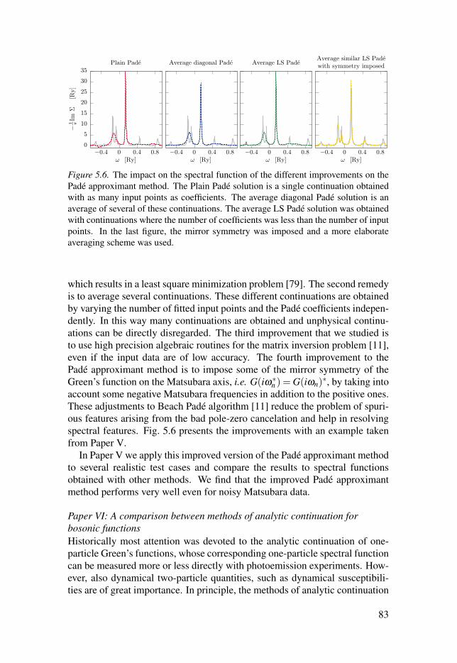
0

5

10

15

20

25

30

35

−0.4 0 0.4 0.8 −0.4 0 0.4 0.8 −0.4 0 0.4 0.8 −0.4 0 0.4 0.8

−1 πIm

Σ[R

y]

ω [Ry]

Plain Pade

ω [Ry]

Average diagonal Pade

ω [Ry]

Average LS Pade

ω [Ry]

Average similar LS Padewith symmetry imposed

Figure 5.6. The impact on the spectral function of the different improvements on the

Padé approximant method. The Plain Padé solution is a single continuation obtained

with as many input points as coefficients. The average diagonal Padé solution is an

average of several of these continuations. The average LS Padé solution was obtained

with continuations where the number of coefficients was less than the number of input

points. In the last figure, the mirror symmetry was imposed and a more elaborate

averaging scheme was used.

which results in a least square minimization problem [79]. The second remedy

is to average several continuations. These different continuations are obtained

by varying the number of fitted input points and the Padé coefficients indepen-

dently. In this way many continuations are obtained and unphysical continu-

ations can be directly disregarded. The third improvement that we studied is

to use high precision algebraic routines for the matrix inversion problem [11],

even if the input data are of low accuracy. The fourth improvement to the

Padé approximant method is to impose some of the mirror symmetry of the

Green’s function on the Matsubara axis, i.e. G(iω∗n ) = G(iωn)∗, by taking into

account some negative Matsubara frequencies in addition to the positive ones.

These adjustments to Beach Padé algorithm [11] reduce the problem of spuri-

ous features arising from the bad pole-zero cancelation and help in resolving

spectral features. Fig. 5.6 presents the improvements with an example taken

from Paper V.

In Paper V we apply this improved version of the Padé approximant method

to several realistic test cases and compare the results to spectral functions

obtained with other methods. We find that the improved Padé approximant

method performs very well even for noisy Matsubara data.

Paper VI: A comparison between methods of analytic continuation forbosonic functionsHistorically most attention was devoted to the analytic continuation of one-

particle Green’s functions, whose corresponding one-particle spectral function

can be measured more or less directly with photoemission experiments. How-

ever, also dynamical two-particle quantities, such as dynamical susceptibili-

ties are of great importance. In principle, the methods of analytic continuation

83

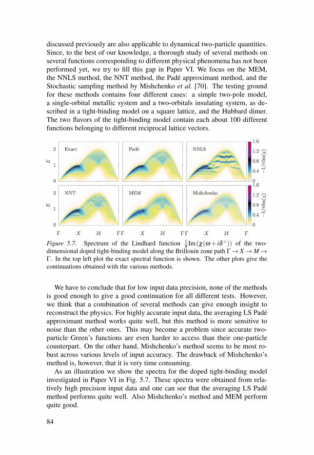
discussed previously are also applicable to dynamical two-particle quantities.

Since, to the best of our knowledge, a thorough study of several methods on

several functions corresponding to different physical phenomena has not been

performed yet, we try to fill this gap in Paper VI. We focus on the MEM,

the NNLS method, the NNT method, the Padé approximant method, and the

Stochastic sampling method by Mishchenko et al. [70]. The testing ground

for these methods contains four different cases: a simple two-pole model,

a single-orbital metallic system and a two-orbitals insulating system, as de-

scribed in a tight-binding model on a square lattice, and the Hubbard dimer.

The two flavors of the tight-binding model contain each about 100 different

functions belonging to different reciprocal lattice vectors.

Figure 5.7. Spectrum of the Lindhard function 1π Im(χ(ω + iδ+)) of the two-

dimensional doped tight-binding model along the Brillouin zone path Γ→ X →M→Γ. In the top left plot the exact spectral function is shown. The other plots give the

continuations obtained with the various methods.

We have to conclude that for low input data precision, none of the methods

is good enough to give a good continuation for all different tests. However,

we think that a combination of several methods can give enough insight to

reconstruct the physics. For highly accurate input data, the averaging LS Padé

approximant method works quite well, but this method is more sensitive to

noise than the other ones. This may become a problem since accurate two-

particle Green’s functions are even harder to access than their one-particle

counterpart. On the other hand, Mishchenko’s method seems to be most ro-

bust across various levels of input accuracy. The drawback of Mishchenko’s

method is, however, that it is very time consuming.

As an illustration we show the spectra for the doped tight-binding model

investigated in Paper VI in Fig. 5.7. These spectra were obtained from rela-

tively high precision input data and one can see that the averaging LS Padé

method performs quite well. Also Mishchenko’s method and MEM perform

quite good.

84

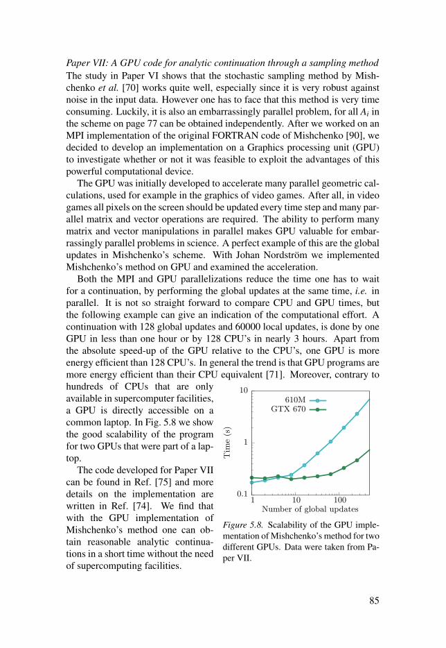
Paper VII: A GPU code for analytic continuation through a sampling methodThe study in Paper VI shows that the stochastic sampling method by Mish-

chenko et al. [70] works quite well, especially since it is very robust against

noise in the input data. However one has to face that this method is very time

consuming. Luckily, it is also an embarrassingly parallel problem, for all Ai in

the scheme on page 77 can be obtained independently. After we worked on an

MPI implementation of the original FORTRAN code of Mishchenko [90], we

decided to develop an implementation on a Graphics processing unit (GPU)

to investigate whether or not it was feasible to exploit the advantages of this

powerful computational device.

The GPU was initially developed to accelerate many parallel geometric cal-

culations, used for example in the graphics of video games. After all, in video

games all pixels on the screen should be updated every time step and many par-

allel matrix and vector operations are required. The ability to perform many

matrix and vector manipulations in parallel makes GPU valuable for embar-

rassingly parallel problems in science. A perfect example of this are the global

updates in Mishchenko’s scheme. With Johan Nordström we implemented

Mishchenko’s method on GPU and examined the acceleration.

Both the MPI and GPU parallelizations reduce the time one has to wait

for a continuation, by performing the global updates at the same time, i.e. in

parallel. It is not so straight forward to compare CPU and GPU times, but

the following example can give an indication of the computational effort. A

continuation with 128 global updates and 60000 local updates, is done by one

GPU in less than one hour or by 128 CPU’s in nearly 3 hours. Apart from

the absolute speed-up of the GPU relative to the CPU’s, one GPU is more

energy efficient than 128 CPU’s. In general the trend is that GPU programs are

more energy efficient than their CPU equivalent [71]. Moreover, contrary to

0.1

1

10

1 10 100

Tim

e(s)

Number of global updates

610MGTX 670

Figure 5.8. Scalability of the GPU imple-

mentation of Mishchenko’s method for two

different GPUs. Data were taken from Pa-

per VII.

hundreds of CPUs that are only

available in supercomputer facilities,

a GPU is directly accessible on a

common laptop. In Fig. 5.8 we show

the good scalability of the program

for two GPUs that were part of a lap-

top.

The code developed for Paper VII

can be found in Ref. [75] and more

details on the implementation are

written in Ref. [74]. We find that

with the GPU implementation of

Mishchenko’s method one can ob-

tain reasonable analytic continua-

tions in a short time without the need

of supercomputing facilities.

85

5.5 Outlook

In Paper V we showed that the Padé approximant method works very well

for one-particle Green’s functions and self-energies. We put a lot of effort

into improving the quality of the continuations even for low precision input

data. We would like to implement our Padé routine into our RSPt code [97]

for two purposes. Firstly, to continue the Green’s function resulting from the

DMFT cycle in order to obtain the spectral function. This feature is needed for

the quantum Monte Carlo and the spin polarized T-matrix fluctuation solver,

since these solvers obtain the Green’s function on the Matsubara axis. The

second application is of a more technical nature. For the exact diagonalization

solver, the hybridization function (see Eq. 2.17 in Sec. 2.3) is fitted with only

a few hybridization parameters. On the Matsubara axis, this function has rel-

atively little structure. It may therefore be worth to analytically continue the

hybridization function to the real axis, fit the few parameters to this function

and use it in the exact diagonalization solver.

Regarding technical improvements of the Padé approximant method, it may

be useful to investigate further the use of some negative Matsubara frequencies

to impose the mirror symmetry of the Green’s function. For the moment we

can say that taking into account some negative frequencies improves the con-

tinuation of one-particle Green’s functions that go to zero for small Matsubara

frequencies, such as the atomic self-energies of Sm and Pr in Paper V. For

metallic Green’s functions, such as the Green’s function of the Bethe lattice,

taking negative iωn into account does not improve the continuation. We be-

lieve that this originates from the discontinuity of the Green’s function when

going from positive to negative Matsubara frequencies for metallic systems

contrary to the continuity for insulating Green’s functions, see Fig. 5.9. Also

for two-particle Green’s functions, taking into account negative frequencies

did not improve the continuation. Relatively broad features are even described

Metallic

Matsubara axis

G(iωn)

Imag Real

Insulating

Matsubara axis

G(iωn)

Imag

Real

Figure 5.9. Sketch of the behavior of metallic and insulating one-particle Green’s

function around iωn = 0. The metallic Green’s function has a discontinuity in the

imaginary part when going from negative to positive Matsubara frequencies.

86

less accurately. We speculate that broad features are usually associated to

branch cuts, which are very difficult to describe with single poles close to the

real axis. We think it would be worth to investigate this issue further to really

pinpoint in which cases negative Matsubara frequencies improve the quality

of the continuations, or if there are other ways to impose mirror symmetry or

favor mirror symmetric solutions.

Although at the moment I do not have any idea on how, it would be impor-

tant to find a more reliable method of analytic continuation for two-particle

Green’s functions. This can be very relevant if one wants to address two-

particle Green’s functions with the three original frequencies (see Eq. 5.3).

In this case, errors associated to the continuation are going to be summed up

when passing to the next frequency.

From a computational point of view, we would like to improve our imple-

mentation [75] of the stochastic sampling method by Mishchenko et al. [70].

We think that using a GPU for this purpose can be highly beneficial, and that

further development of the code would be a good investment. We could also

consider to implement and test different kernels, related to Fredholm equations

in other areas of research.

87

Popular scientific summary

SINCE time immemorial, materials have been important for mankind.

Some prehistoric periods are named after commonly used materials

and the discovery of new materials has always held the potential

of changing the world. Even nowadays, the development of many

applications is restricted by the properties of the materials at our disposal. For

example, why do we not have a laptop that you crease in your pocket like a

handkerchief? Or why do we not have parasols covered with solar cells on

every sunny terrace? This are only a few examples for which we need new

materials with new desired properties. To find these materials, engineers as

well as experimental and theoretical material scientists try to understand the

physics behind these properties and try to figure out where we could find them.

Examples of such properties are transparency, the ability to conduct electric

current, the flexibility or the amount of magnetization. As theoretical material

scientists we aim to calculate these properties and we try to understand the

underlying physics from our calculations. To this aim, we need theoretical

methods. In this work, we try to improve, develop, and test such methods.

However, before describing the three methods and models in this work, we

turn our attention to the materials that we want to describe. All materials

consist of atoms, like lego pirate ships consist of lego bricks. However, atoms

are about 100 million times smaller than a lego brick6. In all materials in

the world, we find only about 100 different type of atoms. Similarly, with

many, but only 100 different types of lego bricks, one could build pirate ships

as well as giraffes or palm trees. The only difference is the way you put the

bricks together. An example on the atomic scale is that both diamond and the

graphite stick in your pencil, consist of solely carbon atoms. They differ only

by the stacking of these atoms! If we focus on the atoms again, they, in turn,

consists of a nucleus surrounded by electrons. The electrons are attracted by

the nucleus, but repelled by one an other. In this thesis we try to understand

and predict the properties of materials from this atomic scale, by describing

the behavior of the electrons.

This thesis consists of three parts, where we consider three different meth-

ods or models:

1. A method to describe the electronic structure of the rare earthsWhen we put atoms together, to build a material, these electrons can stay close

6The lego brick of course consists of atoms itself.

88

to the nucleus, or they can wander around in the material, hopping from nu-

cleus to nucleus. The behavior of the electrons depends on the type of atom

they belong to. In the rare-earth elements, which are a specific class of atoms,

some of the electrons wander around and some stay very close to their nu-

cleus. It turned out, that this is very hard to properly describe theoretically.

The common theoretical tool to describe the electronic structure of materials

is called density functional theory. This method works very well for many

types of atoms, but precisely for the rare earths is does not work so well. This

is due to the fact that the electrons that stay close to the nucleus feel a strong

repulsion from one an other. Density functional theory describes this repul-

sion only partially and for the rare earths this repulsion needs to be taken into

account explicitly. In this thesis we examined and analyzed a way to take this

into account: the Hubbard I approximation. In this work we show that this

method works very well to describe the rare-earth elements. These elements

are used in strong permanent magnets as can be found in, for example, wind-

mills and electric cars.

2. A model to predict the microscopic state after ultrafast magnetization dy-namicsSome atoms can act like a tiny magnet, with a south pole on one end, and a

north pole on the other end. All these tiny little magnets constitute a total mag-

netization in a material. Experimentalists can flash an ultrashort laser pulse

onto such a material, to probe its characteristics. By measuring the amount

of light that is reflected, they can measure the magnetization of the material.

It turns out that the material under some circumstances can lose part of its

magnetization and, in other circumstances, can gain additional magnetization

due to the ultrashort flash. The magnetization is a macroscopic quantity of

the entire sample, but to understand the physics, it is interesting to look at the

atomic scale. With our model, we predict what happens to the tiny atomic

magnetic moments in both cases, i.e. the growth and decrease of magnetiza-

tion. We find that the atomic magnetic moments increase in strength when

the total magnetization increases. When the total magnetization decreases, the

atomic magnetic moments keep their strength, but they tilt in various direc-

tions. We use our predictions on the atomic scale to calculate the macroscopic

quantities that the experimentalists measure. In this way the experiments can

confirm our model and our model can explain the experiments.

3. Different methods of analytic continuationMaterials are described by their electronic structure, the behavior of the elec-

trons around the nucleus. For materials where some of the electrons wander

around and some stay very close to their nucleus, is is not so easy to make

good theoretical predictions of this behavior. Most methods that aim to do

this, calculate the electronic structure as a function of imaginary time. This

sounds very fancy, but it is mainly a mathematical trick to make the calcula-

89

tions easier. However, to obtain real physical quantities, which are a function

of real energies, one needs a method of analytic continuation. In our work

we extensively tested several methods of analytic continuation and improved

some of them for the particular needs in this area of research.

With our work on these methods and models we hope to contribute to the

improvement of the state-of-the-art methods used in material science.

90

Populärvetenskaplig sammanfattning

SEDAN urminnes tider, har material varit viktiga för mänskligheten.

Några förhistoriska perioder är namngivna efter använda material

under den eran och upptäckten av nya material har alltid haft poten-

tialen att förändra världen. Även idag är utvecklingen av nya appli-

kationer begränsade av egenskaperna hos de material som finns tillgängliga.

Till exempel, varför har vi inte bärbara datorer som man kan vika ihop likt

en näsduk? Eller varför har vi inte parasoll som är täckta av solceller på var-

je solig terrass? Detta är bara några få exempel där vi behöver nya material

med nya materialegenskaper. För att upptäcka dessa material försöker ingen-

jörer och materialforskare förstå fysiken bakom dessa egenskaper. Exempel

på sådana egenskaper är genomskinlighet, elektrisk ledningsförmåga, flexi-

bilitet och magnetiseringsstyrka. Som teoretiska materialforskare försöker vi

beräkna dessa egenskaper och förstå den underliggande fysiken genom våra

beräkningar. För att lyckas med detta behöver vi teoretiska metoder. I denna

avhandling försöker vi förbättra, utveckla och testa sådana metoder.

Innan vi beskriver de tre metoderna och modellerna i denna avhandling

fokuserar vi först på materialen som vi vill beskriva. Alla material består av

atomer, likt piratskepp i lego består av legobitar. Dock är atomer ungefär 100

miljoner gånger mindre än en legobit7. I alla material i världen finner vi bara

ungefär 100 olika typer av atomer. I liknelsen med legor kan vi med enbart

dessa typer bygga piratskepp, giraffer eller palmträd, den enda skillnaden är

hur man sätter ihop bitarna. Ett exempel på atomskalan är att diamant och

blyertspennor båda bara består av kolatomer, de skiljer sig bara i hur atomerna

är strukturerade! Om vi återigen fokuserar på atomerna, består de i sin tur

av en atomkärna och omgivande elektroner. Elektronerna är attraherade till

atomkärnan, men repelleras av varandra. I denna avhandling försöker vi förstå

och förutsäga materialegenskaperna från denna atomskala genom att beskriva

elektronernas beteende.

Denna avhandling består av tre delar, innehållande tre metoder eller model-

ler:

1. En metod för att beskriva elektronstrukturen av de sällsynta jordartsmetal-lernaNär vi för samman atomer för att bygga material, kan dessa elektroner stanna

nära atomkärnan eller vandra omkring i materialet, hoppandes från atomkär-

na till atomkärna. Beteendet av elektronerna beror på vilken sorts atom de

7Legobiten består såklart själv av atomer.

91

tillhör. I de sällsynta jordartsmetallerna, vilka är en särskild klass av atomer,

kommer några elektroner att vandra omkring och några att stanna väldigt nä-

ra dess atomkärna. Detta har visat sig vara väldigt svårt att beskriva teore-

tiskt. En vanlig teoretisk metod för att beskriva elektronstrukturen av material

kallas täthetsfunktionalteori. Denna metod fungerar väldigt bra för många ty-

per av atomer, men inte för de sällsynta jordartsmetallerna. Detta beror på att

elektronerna som är nära atomkärnan känner en stark repulsion från varand-

ra. Täthetsfunktionalteori beskriver enbart delvis denna repulsion och för de

sällsynta jordartsmetallerna behöver man explicit behandla effekten av denna

repulsion. I denna avhandling studerar och analyserar vi ett tillvägagångsätt

för att göra detta: Hubbard I approximationen. I detta arbete visar vi att den-

na metod fungerar väldigt bra för att beskriva de sällsynta jordartsmetallerna.

Dessa ämnen används i starka permanent magneter, till exempel i vindkraft-

verk och i elektriska bilar.

2. En modell för att förutsäga det mikroskopiska tillståndet efter ultrasnabbmagnetiseringsdynamikVissa atomer kan bete sig som små magneter, med en sydpol och en nord-

pol. Alla dessa små magneter utgör en total magnetisering i materialet. Ex-

perimentalister kan stråla en ultrakort laserpuls på ett sådant material, för att

utröna dess egenskaper. Genom att mäta mängden ljus som reflekteras kan

de uppmäta magnetiseringen i materialet. Det visar sig att materialet under

vissa omständigheter kan förlora delar av sin magnetisering och under and-

ra förhållanden få en ökad magnetisering, på grund av den kort laserpulsen.

Magnetiseringen är en makroskopisk kvantitet för hela provbiten, men för att

förstå fysiken är det intressant att betrakta på den atomistiska skalan. Med

vår modell förutsäger vi vad som händer med de små magnetiska momenten

i båda fallen, det vill säga för ökad och minskad magnetisering. Vi inser att

de magnetiska momenten ökar då den totala magnetiseringen ökar. När den

totala magnetiseringen minskar, behåller de atomiska magnetiska momenten

sin styrka, men de vrider sig till olika riktningar. Vi använder våra förutsägel-

ser på den atomiska skalan för att beräkna de makroskopiska kvantiteter som

experimentalisterna mäter. På detta sätt kan experimenten bekräfta vår modell

och vår modell kan förklara experimenten.

3. Olika metoder för analytisk fortsättningMaterial beskrivs av dess elektronstruktur, det vill säga elektronernas beteen-

de omkring atomkärnan. För material där vissa elektroner vandrar omkring

och några är väldigt nära dess atomkärna är det svårt att göra bra teoretiska

förutsägelser för detta beteende. De flesta metoder som försöker modellera

detta beräknar elektronstrukturen som en funktion av imaginär tid. Detta låter

väldigt komplext men det är förförallt ett matematiskt trick för att förenkla

beräkningarna. Men för att erhålla verkliga kvantiteter, som beror på verkliga

energier, behöver man en metod för analytisk fortsättning. I vårt arbete har vi

92

noggrant testat flera metoder för analytisk fortsättning och förbättrat några av

dem, baserat på behoven i detta forskningsfält.

Med vårt arbete på dessa metoder och modeller hoppas vi bidra till att för-

bättra toppmoderna metoder i materialforskning.

93

Populair wetenschappelijke samenvatting

SINDS mensenheugenis zijn materialen belangrijk voor de mensheid.

Enkele prehistorische perioden zijn zelfs vernoemd naar veelgebruikte

materialen van die tijd. De ontdekking van nieuwe materialen kan

zorgen voor grote veranderingen in de wereld. Ook de ontwikkeling

van moderne technologie wordt nog steeds begrensd door de eigenschappen

van de materialen die we ervoor kunnen gebruiken. Waarom hebben we bij-

voorbeeld geen laptop die we als een zakdoek in onze broekzak kunnen from-

melen? Of waarom hebben we geen zonnecellen op de parasols op de vele

zonnige terrasjes? Dit zijn slechts enkele voorbeelden van toepassingen waar

we nieuwe materialen voor nodig zouden hebben met nieuwe gewenste eigen-

schappen. Om deze materiaaleigenschappen te vinden, proberen technici en

experimentele en theoretische materiaalwetenschappers de natuurkunde ach-

ter materialen te begrijpen. Zij proberen uit te zoeken waar we de gewenste

eigenschappen kunnen vinden. Enkele voorbeelden van dit soort eigenschap-

pen zijn transparantie, de mogelijkheid om elektrische stroom te geleiden, de

flexibiliteit van het materiaal of de hoeveelheid magnetisatie in het materiaal.

Het doel van theoretische materiaalwetenschappers is het berekenen van deze

eigenschappen en het begrijpen van de onderliggende natuurkunde vanuit deze

berekeningen. Om dit doel te bereiken hebben we theoretische modellen en

methodes nodig. In dit proefschrift proberen we dit soort methodes te verbe-

teren en te ontwikkelen.

Voordat we verder ingaan op de drie methodes en modellen in dit proef-

schrift, kijken we even naar de materialen die we uiteindelijk willen beschrij-

ven. Alle materialen bestaan uit atomen, net als legopiratenschepen bestaan

uit kleine legoblokjes. Atomen zijn echter ongeveer 100 miljoen keer kleiner

dan legoblokjes8. In alle materialen op aarde komen slechts ongeveer honderd

verschillende atomen voor. Zo kun je ook, met een doos legoblokjes waar

slecht honderd verschillende soorten blokjes inzitten, zowel een piratenschip

bouwen als ook een giraffe of een paar palmbomen. Het verschil zit ’m slechts

in hoe je de blokjes op elkaar drukt. Een voorbeeld op atomaire schaal is dat

zowel diamant als de grafietstaaf in je potlood, enkel uit koolstofatomen be-

staat. Het enige verschil is de manier waarop de atomen op elkaar gestapeld

zijn!

Wanneer we nu naar de atomen zelf kijken, zien we dat deze bestaan uit

een kern, omringd door elektronen. De elektronen worden aangetrokken door

8Legoblokjes bestaan natuurlijk zelf ook uit atomen.

94

de kern, maar stoten elkaar juist af. In dit proefschrift proberen we de eigen-

schappen van materialen op deze atomaire schaal te begrijpen en te voorspel-

len, door te kijken naar het gedrag van de elektronen.

Dit proefschrift bestaat uit drie delen waarin we drie verschillende metho-

des of modellen bekijken:

1. Een methode om de elektronenstructuur van de zeldzame aardmetalen tebeschrijvenWanneer we de atomen stapelen om een materiaal te vormen, kunnen de elek-

tronen dicht bij hun kern blijven, of juist vrij door het materiaal heen bewegen,

al springend van kern naar kern. Het gedrag van de elektronen hangt af van

het atoom waar ze toe behoren. De zeldzame aardmetalen zijn een bepaalde

groep atomen. Deze atomen worden bijvoorbeeld gebruikt in sterke perma-

nente magneten die hun toepassing vinden in, bijvoorbeeld, windmolens en

elektrische auto’s. Bij deze groep atomen zijn er enkele elektronen die zich

vrij door het gehele materiaal bewegen en enkele die dicht bij hun eigen kern

blijven. Het blijkt, dat het erg lastig is om dit theoretisch te beschrijven. De

meest gebruikte theoretische methode voor het beschrijven van de elektro-

nenstructuur van materialen heet dichtheidsfunctionaaltheorie. Deze methode

werk voor veel atoomsoorten heel goed, maar juist voor de zeldzame aard-

metalen niet zo goed. Dit komt omdat de elektronen die bij hun eigen kern

blijven ook dicht bij elkaar zijn en daarom een sterke afstotende kracht van

elkaar voelen. Dichtheidsfunctionaaltheorie beschrijft deze kracht slechts ge-

deeltelijk en voor de zeldzame metalen moet deze afstotende kracht expliciet

meegenomen worden in de berekeningen. In dit proefschrift onderzoeken en

analyseren we een manier om dit te doen: de Hubbard I benadering. We laten

zien dat deze methode goed werkt om de zeldzame aardmetalen te beschrijven.

2. Een model om de microscopische toestand na ultrasnelle magnetisatiedy-namica te voorspellenSommige atomen zijn net kleine magneetjes, met een zuidpool aan de ene kant

en een noordpool aan de andere kant. Al deze kleine magneetjes vormen te-

zamen de totale magnetisatie van het materiaal. Om de eigenschappen van

zo’n materiaal te onderzoeken, kunnen experimentelen een ultrakorte laser-

puls op zo’n materiaal flitsen. Door de hoeveelheid licht te meten die wordt

gereflecteerd, kunnen ze de magnetisatie van het materiaal bepalen. Het blijk

dat het materiaal, door een felle laserflits, een deel van zijn magnetisatie kan

verliezen, terwijl het onder andere omstandigheden juist extra magnetisatie

krijgt. De magnetisatie is een eigenschap van het hele materiaal, maar om de

natuurkunde te begrijpen is het interessant om op atomaire schaal te kijken

wat er gebeurt. Met ons model voorspellen we wat er gebeurt met de kleine

atomaire magneetjes in beide gevallen, namelijk tijdens de groei en de krimp

van de magnetisatie. We laten zien dat de atomaire magneetjes sterker worden

wanneer de totale magnetisatie groter wordt. Wanneer de totale magnetisatie

95

kleiner wordt, zullen de atomaire magneetjes even sterk blijven, maar naar ver-

schillende richtingen kantelen. We gebruiken onze voorspellingen op atomaire

schaal om de macroscopische grootheden te berekenen die de experimentelen

kunnen meten. Op deze manier kunnen experimentele metingen ons model

bevestigen en kan ons model de metingen verklaren.

3. Verschillende methodes voor analytische voortzettingMaterialen worden beschreven door hun elektronenstructuur, het gedrag van

de elektronen rond hun kern. Voor de materialen waar sommige elektronen

zich vrij rond bewegen en andere elektronen juist dicht bij hun kern blijven,

is het niet zo makkelijk om goede theoretische voorspellingen over dit gedrag

te doen. De meeste methodes die dit doen, berekenen de elektronenstructuur

as een functie van imaginaire tijd. Dit klinkt heel ingewikkeld, maar het is

slechts een wiskundig trucje om de berekeningen makkelijker te maken. Het

is echter wel belangrijk om aan het einde van de rit weer terug te keren naar

echte energie in plaats van imaginaire tijd en daarvoor hebben we een me-

thode voor analytische voortzetting nodig. In dit proefschrift testen we een

aantal methodes voor analytische voorzetting uitgebreid. We verbeteren en-

kele van deze methodes voor de specifieke behoeftes in dit onderzoeksgebied.

We hopen met het werk dat we in dit proefschrift hebben gedaan, een bij-

drage te leveren aan de “state-of-the-art” methodes in de materiaalwetenschap.

96

Acknowledgements

Iam extremely grateful when I reflect upon my time in Uppsala. I got so

lucky to meet so many friendly and inspiring people. Here follows only

a short list of them.

First of all I would like to thank my supervisors in Uppsala, Igor and

Olle. Igor, I think it was really great to work with you. Despite all obstacles,

you are always positive, happy and enthusiastic. You were always willing to

discuss, to give some new input and to help me. You gave me the feeling

that it was save to try and to fail and to try again. I always felt supported

and appreciated by you. I think we had a good collaboration, although, our

clocks, somehow, never showed the same time. And very important: we had

fun. Thanks a lot!

Olle, it was great to work on a project that lies so close to your heart. More-

over, I think you are the best boss I ever had or even will have. You are always

optimistic, enthusiastic and full of ideas. You have so many suggestions for

projects and collaborations that it is hard to choose the nicest. As important as

your scientific input, I think, is that you really care about your students, post-

docs and other colleagues. You care about their well-being and about their

future. You encourage social cohesion in our group. With this, I think, you

create a very nice atmosphere. I also would like to thank my supervisors for

encouraging me to do a joint doctorate with the Radboud University in Ni-

jmegen.

Also I would like to thank my supervisors Misha and Annalisa in Nijmegen.

Misha, with your vast amount of scientific knowledge and deep understanding

you can guide people in good directions. Annalisa, we did not collaborate

closely during my PhD, but you always cared about me and guided me in the

world of academia.

I think that the material theory group in Uppsala is really very special. I

would like to thank all people in my group, for making my work, the lunches

and the fika so enjoyable. I’m very grateful to all of you, but some people I

would like to thank personally. Iulia and Alex, thanks a lot for the nice jug-

gling hours. I would like to thank my office mates. Samara, I learned a lot

from you about Iran and also about myself. Johan, I really enjoyed working

with you on our analytic continuation projects. For me it was a lot of fun,

sitting together, going through your huge amount of data, structuring and or-

dering it in order to draw conclusions. Marco, you were also a bit an office

mate, but mainly a great collaborator. Your tendency to start an explanation at

the very beginning with, “Do you know what electrons are?”, was really great

97

when I just started my PhD and knew close to nothing. I really like your intu-

itive way of thinking and explaining. Your enthusiastic and passionate debates

together with Igor were funny and inspiring at the same time. In this list, I

finally would like to thank Yaroslav, you are among the kindest people I know.

You were always in for discussions and it was very nice to figure out things

together with you as we did, for example, with the multiplet structure of the

REs.

In Uppsala I, furthermore, would like to thank the DMFT subgroup. It is

very inspiring and useful when more people work on related problems with

similar methods. The same holds for my direct collaborators, many thanks to

all of you. A special thanks to Marco, Erik, Johan Nordström, Johan Schött,

Elin, Debora, Manuel, Anna, Somnath, Ronny and Yaroslav.

In Nijmegen I would like to thank the TCM department for hosting me.

Lars, Jaap en Alessandro thanks for the help, the discussions and the nice cof-

fee. Guus, Merel, Remko, Lennert, Erik, Koen, Linde and all group members,

thanks for the nice time we had.

Doing a PhD in Uppsala, is not only about science, but also about living

alone in Sweden for more than four years. This has not always been easy.

If it were not for the wonderful job I had, the great group I worked in, and

not the least all friends that supported me, I am not sure I would have done

it. I would like to thank all friends that visited me, sometimes even in winter

or in the dark November month. Dank je wel Margot, Dirk, Linde, Laura,

Lizzy, Jan, Heike, Rebekka, Nora, Maartje, Joost, Roos, Wim, Nadia, Maurits,

Merel, Jins, Lennert en Erik. Liebe Oma, Silke und Fritz, vielen Dank für euer

Besuch. I have many good memories of cups of warm tea, of great walks in

stadsskogen and Hågadalen-Nåstens nature, of swimming, of Stockholm, of

baking cookies and of hours of peaceful knitting. Linde, thanks a lot for all the

phone calls, I could always count on your advise and encouragement. Pappa,

mamma and Margot thanks a lot for jumping on the plane when I needed you

the most.

I would also like to thank the best roommates ever: Delphine, Kim, Maciej,

Wojciech and Sara. I have had so many good evenings, nice barbecues, good

backing experiences and cat-chat with you! Sasha and Yaroslav, here is a

special thanks to you, it is really great to have some friends that are there

when you need them. Everything is good in the end, but sometimes you need

friends to remind you.

Jord, thank you very much for all your support, for all the times you came

to visit me and for this four and a half years of waiting for me. From now on,

we will finally live together again.

98

Appendices

99

A. Finding the multiplets in Nd

Here we present a recipe to construct the multiplets in the valence band spec-

trum, with the XPS spectrum of Nd as example. The f 3 → f 2 transitions

are complicated enough to be able to extend it to more electrons, but simple

enough to keep the bookkeeping doable. I have probably learned the recipe

in my undergraduate studies, but unfortunately I have also forgotten it. . . For

me learning it again made a lot of things clearer. Therefore I wrote down the

example of Nd.

Step 1: Write down all the ways in which one can divide two electrons over7 orbitals or 14 spin orbitals. This can be done in 14∗13

2 = 91 ways, which are

listed compactly in Tab. A.1 by dividing them into 5 groups. The first group is

special, it contains a pair of spin up and spin down in one orbital, which can

be ml = −3,−2,−1,0,1,2 or 3. The second group considers two spin up in

different orbitals. The first spin up can be in ml =−3,−2,−1,0,1,2,3 and the

second can be in all possible orbitals with ml bigger than that of the first. The

other three groups have the same form, but with one up and one down, with

one down and one up, and finally with two spin down electrons.

Step 2: Construct a table denoting how many states we have for each Szand Lz. The Nd example is given in Tab. A.2.

Step 3: Obtain the possible S,L multiplets from the previous table. Start

with the highest possible Sz and Lz, subtract this from the table and continue

till all multiplets are specified and only zero’s are left in the table. In the

Nd example (Tab. A.3 till A.9) we take: L = 6 (highest possible Lz = 6) for

which we only have Sz = 0⇒ S = 0 (Tab. A.3→ A.4); S = 1, L = 5 (Tab. A.4

→ A.5); and so forth (Tab. A.5 till A.9). This procedure gave us the following

multiplets, which are highlighted in blue in the tables: 1I6, 3H4,5,6, 1G4, 1S0,3F2,3,4, 1D2 and 3P0,1,2.

100

Table A.1. All possible ways to divide two electrons in 7 orbitals denoted with −3≤ml ≤ 3. The states are grouped, such that the red arrow can be also in the position ofthe red dots. The total Sz and Lz are given in the subsequent columns. All possibilitiesfor Lz are listed, depending on where the red arrow is. In the last column the numberof states in this group is given. The total number of states is 21+21+21+21+7= 91

as expected.

-3 -2 -1 0 1 2 3 Sz Lz #

↑↓ . . . . . . . . . . . . . . . . . . 0 -6,-4, -2,0,2,4,6 7

↑ ↑ . . . . . . . . . . . . . . . 1 -5, -4,-3,-2,-1,0 21

↑ ↑ . . . . . . . . . . . . -3, -2, -1,0,1

↑ ↑ . . . . . . . . . -1,0,1,2

↑ ↑ . . . . . . 1,2,3

↑ ↑ . . . 3,4

↑ ↑ 5

Same for ↑ ↓ 0 -5,-4,-3,-2,-1,0, 21

-3,-2,-1,0,1,-1,0,1,2,

1,2,3,3,4,5

Same for ↓ ↑ 0 -5,-4,-3,-2,-1,0, 21

-3,-2,-1,0,1,-1,0,1,2,

1,2,3,3,4,5

Same for ↓ ↓ -1 -5,-4,-3,-2,-1,0, 21

-3,-2,-1,0,1,-1,0,1,2,

1,2,3,3,4,5

Table A.2. Number of states with all possible Sz and Lz.

Sz \Lz -6 -5 -4 -3 -2 -1 0 1 2 3 4 5 6

-1 0 1 1 2 2 3 3 3 2 2 1 1 0

0 1 2 3 4 5 6 7 6 5 4 3 2 1

1 0 1 1 2 2 3 3 3 2 2 1 1 0

Table A.3. S = 0 and L = 6 multiplet 1I6.

Sz \Lz -6 -5 -4 -3 -2 -1 0 1 2 3 4 5 6

-1 0 1 1 2 2 3 3 3 2 2 1 1 0

0 1 2 3 4 5 6 7 6 5 4 3 2 1

1 0 1 1 2 2 3 3 3 2 2 1 1 0

101

Table A.4. S = 1 and L = 5 multiplet 3H4,5,6.

Sz \Lz -6 -5 -4 -3 -2 -1 0 1 2 3 4 5 6

-1 0 1 1 2 2 3 3 3 2 2 1 1 0

0 0 1 2 3 4 5 6 5 4 3 2 1 0

1 0 1 1 2 2 3 3 3 2 2 1 1 0

Table A.5. S = 0 and L = 4 multiplet 1G4.

Sz \Lz -6 -5 -4 -3 -2 -1 0 1 2 3 4 5 6

-1 0 0 0 1 1 2 2 2 1 1 0 0 0

0 0 0 1 2 3 4 5 4 3 2 1 0 0

1 0 0 0 1 1 2 2 2 1 1 0 0 0

Table A.6. S = 1 and L = 3 multiplet 3F2,3,4.

Sz \Lz -6 -5 -4 -3 -2 -1 0 1 2 3 4 5 6

-1 0 0 0 1 1 2 2 2 1 1 0 0 0

0 0 0 0 1 2 3 4 3 2 1 0 0 0

1 0 0 0 1 1 2 2 2 1 1 0 0 0

Table A.7. S = 0 and L = 2 multiplet 1D2.

Sz \Lz -6 -5 -4 -3 -2 -1 0 1 2 3 4 5 6

-1 0 0 0 0 0 1 1 1 0 0 0 0 0

0 0 0 0 0 1 2 3 2 1 0 0 0 0

1 0 0 0 0 0 1 1 1 0 0 0 0 0

Table A.8. S = 1 and L = 1 multiplet 3P0,1,2.

Sz \Lz -6 -5 -4 -3 -2 -1 0 1 2 3 4 5 6

-1 0 0 0 0 0 1 1 1 0 0 0 0 0

0 0 0 0 0 0 1 2 1 0 0 0 0 0

1 0 0 0 0 0 1 1 1 0 0 0 0 0

Table A.9. S = 0 and L = 0 multiplet 1S0.

Sz \Lz -6 -5 -4 -3 -2 -1 0 1 2 3 4 5 6

-1 0 0 0 0 0 0 0 0 0 0 0 0 0

0 0 0 0 0 0 0 1 0 0 0 0 0 0

1 0 0 0 0 0 0 0 0 0 0 0 0 0

102

References

[1] http://elk.sourceforge.net/.

[2] O. K. Andersen. Linear methods in band theory. Phys. Rev. B, 12:3060–3083,

1975.

[3] O. K. Andersen and R. V. Kasowski. Electronic states as linear combinations

of muffin-tin orbitals. Phys. Rev. B, 4:1064–1069, 1971.

[4] Vladimir I. Anisimov, Jan Zaanen, and Ole K. Andersen. Band theory and

Mott insulators: Hubbard U instead of Stoner I. Phys. Rev. B, 44:943–954,

1991.

[5] P. Anthony Cox. Fractional parentage methods for ionisation of open shells of

d and f electrons. In Photoelectron Spectrometry, volume 24 of Structure andBonding, pages 59–81. Springer Berlin Heidelberg, 1975.

[6] V. P. Antropov, M. I. Katsnelson, B. N. Harmon, M. van Schilfgaarde, and

D. Kusnezov. Spin dynamics in magnets: Equation of motion and finite

temperature effects. Phys. Rev. B, 54:1019–1035, 1996.

[7] Neil W. Ashcroft and N. David Mermin. Solid state physics. Saunders

College, Philadelphia, 1976.

[8] G. A. Baker. Essentials of Padé Approximants. Academic Press, New York,

1975.

[9] M. Battiato, K. Carva, and P. M. Oppeneer. Superdiffusive spin transport as a

mechanism of ultrafast demagnetization. Phys. Rev. Lett., 105:027203, 2010.

[10] M. Battiato and K. Held. Ultrafast and gigantic spin injection in

semiconductors. Phys. Rev. Lett., 116:196601, 2016.

[11] K. S. D. Beach, R. J. Gooding, and F. Marsiglio. Reliable padé analytical

continuation method based on a high-accuracy symbolic computation

algorithm. Phys. Rev. B, 61:5147–5157, 2000.

[12] E. Beaurepaire, J.-C. Merle, A. Daunois, and J.-Y. Bigot. Ultrafast spin

dynamics in ferromagnetic nickel. Phys. Rev. Lett., 76:4250–4253, 1996.

[13] Francis Birch. Finite elastic strain of cubic crystals. Phys. Rev., 71:809–824,

1947.

[14] Torbjörn Björkman. Magnetic and Structural Properties of f-electron Systemsfrom First Principles Theory. PhD thesis, Uppsala University, 2009.

[15] Felix Bloch. Über die quantenmechanik der elektronen in kristallgittern.

Zeitschrift für Physik, 52(7-8):555–600, 1929.

[16] M. Born and R. Oppenheimer. Zur quantentheorie der molekeln. Ann. Phys.,389(20):457–484, 1927.

[17] D. H. Brooks and R. S. MacLeod. Electrical imaging of the heart. IEEE SignalProcessing Magazine, 14(1):24–42, 1997.

[18] K. H. J. Buschow. Handbook of magnetic materials. Vol. 13. Elsevier,

Amsterdam, 2001.

103

[19] Robert Carley, Kristian Döbrich, Björn Frietsch, Cornelius Gahl, Martin

Teichmann, Olaf Schwarzkopf, Philippe Wernet, and Martin Weinelt.

Femtosecond laser excitation drives ferromagnetic gadolinium out of magnetic

equilibrium. Phys. Rev. Lett., 109:057401, 2012.

[20] Stanislav Chadov. Application of many-body perturbation theory to the

description of correlated metals, 2007.

[21] C Cheng, R J Needs, and V Heine. Inter-layer interactions and the origin of

SiC polytypes. Journal of Physics C: Solid State Physics, 21(6):1049, 1988.

[22] P A Cox, J K Lang, and Y Baer. Study of the 4f and valence band density of

states in rare-earth metals. I. theory of the 4f states. Journal of Physics F:Metal Physics, 11(1):113, 1981.

[23] F. Dalla Longa, J. T. Kohlhepp, W. J. M. de Jonge, and B. Koopmans.

Influence of photon angular momentum on ultrafast demagnetization in nickel.

Phys. Rev. B, 75:224431, 2007.

[24] P. H. Dederichs, S. Blügel, R. Zeller, and H. Akai. Ground states of

constrained systems: Application to cerium impurities. Phys. Rev. Lett.,53:2512–2515, 1984.

[25] Anna Delin, Lars Fast, Börje Johansson, Olle Eriksson, and J. M. Wills.

Cohesive properties of the lanthanides: Effect of generalized gradient

corrections and crystal structure. Phys. Rev. B, 58:4345–4351, 1998.

[26] P J H Denteneer and W van Haeringen. Stacking-fault energies in

semiconductors from first-principles calculations. Journal of Physics C: SolidState Physics, 20(32):L883, 1987.

[27] Igor Di Marco. Correlation Effects in the Electronic Structure of TransitionMetals and Their Compounds. PhD thesis, Radboud University Nijmegen,

Ipskamp Drukkers, Enschede, The Netherlands, 2009.

[28] F Drymiotis, J Singleton, N Harrison, J C Lashley, A Bangura, C H Mielke,

L Balicas, Z Fisk, A Migliori, and J L Smith. Suppression of the γ-α structural

phase transition in Ce0.8La0.1Th0.1 by large magnetic fields. Journal ofPhysics: Condensed Matter, 17(7):L77, 2005.

[29] H Ebert. Magneto-optical effects in transition metal systems. Reports onProgress in Physics, 59(12):1665, 1996.

[30] Olle Eriksson, M. S. S. Brooks, and Börje Johansson. Orbital polarization in

narrow-band systems: Application to volume collapses in light lanthanides.

Phys. Rev. B, 41:7311–7314, 1990.

[31] Michael Faraday. Experimental researches in electricity. nineteenth series.

Philosophical Transactions of the Royal Society of London, 136:1–20, 1846.

[32] Raymond Frésard and Gabriel Kotliar. Interplay of mott transition and

ferromagnetism in the orbitally degenerate hubbard model. Phys. Rev. B,

56:12909–12915, 1997.

[33] Antoine Georges. Strongly correlated electron materials: Dynamical

mean-field theory and electronic structure. AIP Conference Proceedings,

715(1):3–74, 2004.

[34] Khaldoon Ghanem. Stochastic Mode Sampling (SMS) – An Efficient

Approach to the Analytic Continuation Problem. Ms, RWTH Aachen, 2013.

RWTH Aachen, Masterarbeit, 2013.

[35] Roberta Grech, Tracey Cassar, Joseph Muscat, Kenneth P Camilleri, Simon G

104

Fabri, Michalis Zervakis, Petros Xanthopoulos, Vangelis Sakkalis, and Bart

Vanrumste. Review on solving the inverse problem in EEG source analysis.

Journal of NeuroEngineering and Rehabilitation, 5:25–25, 2008.

[36] W. A. Grosshans and W. B. Holzapfel. Atomic volumes of rare-earth metals

under pressures to 40 GPa and above. Phys. Rev. B, 45:5171–5178, 1992.

[37] G. Grosso and G.P. Parravicini. Solid State Physics. Academic Press, 2000.

[38] K.A. Gschneidner. Physical properties of the rare earth metals. Bulletin ofAlloy Phase Diagrams, 11(3):216–224, 1990.

[39] Karl A. Gschneidner and LeRoy Eyring. Handbook on the physics andchemistry of rare earths. Vol. 1, Metals. Amsterdam, 1978.

[40] Karl A. jr. Gschneidner and LeRoy Eyring. Handbook on the physics andchemistry of rare earths. Vol. 10, High energy spectroscopy. Amsterdam, 1987.

[41] O. Gunnarsson, J. W. Allen, O. Jepsen, T. Fujiwara, O. K. Andersen, C. G.

Olsen, M. B. Maple, J.-S. Kang, L. Z. Liu, J.-H. Park, R. O. Anderson, W. P.

Ellis, R. Liu, J. T. Markert, Y. Dalichaouch, Z.-X. Shen, P. A. P. Lindberg,

B. O. Wells, D. S. Dessau, A. Borg, I. Lindau, and W. E. Spicer. Polarized

resonance photoemission for Nd2CuO4. Phys. Rev. B, 41:4811–4814, 1990.

[42] O. Gunnarsson, O. K. Andersen, O. Jepsen, and J. Zaanen. Density-functional

calculation of the parameters in the Anderson model: Application to Mn in

CdTe. Phys. Rev. B, 39:1708–1722, 1989.

[43] P. C. Hansen. The L-curve and its use in the numerical treatment of inverse

problems. In in Computational Inverse Problems in Electrocardiology, ed. P.Johnston, Advances in Computational Bioengineering, pages 119–142. WIT

Press, 2000.

[44] K. Held. Electronic structure calculations using dynamical mean field theory.

Advances in Physics, 56(6):829–926, 2007.

[45] P. Hohenberg and W. Kohn. Inhomogeneous electron gas. Phys. Rev.,136:B864–B871, 1964.

[46] J. Hubbard. Electron correlations in narrow energy bands. Proceedings of theRoyal Society of London A: Mathematical, Physical and Engineering Sciences,

276(1365):238–257, 1963.

[47] J. Hubbard. Electron correlations in narrow energy bands. II. the degenerate

band case. Proceedings of the Royal Society of London A: Mathematical,Physical and Engineering Sciences, 277(1369):237–259, 1964.

[48] J. Hubbard. Electron correlations in narrow energy bands. III. an improved

solution. Proceedings of the Royal Society of London A: Mathematical,Physical and Engineering Sciences, 281(1386):401–419, 1964.

[49] Christian Illg, Michael Haag, and Manfred Fähnle. Ultrafast demagnetization

after laser irradiation in transition metals: Ab initio calculations of the spin-flip

electron-phonon scattering with reduced exchange splitting. Phys. Rev. B,

88:214404, 2013.

[50] Mark Jarrell and J.E. Gubernatis. Bayesian inference and the analytic

continuation of imaginary-time quantum Monte Carlo data. Physics Reports,

269(3):133 – 195, 1996.

[51] Jens Jensen and Allan R. Mackintosh. Rare earth magnetism. Clarendon

Press, Oxford, 1991.

[52] Börje Johansson and Anders Rosengren. Generalized phase diagram for the

105

rare-earth elements: Calculations and correlations of bulk properties. Phys.Rev. B, 11:2836–2857, 1975.

[53] Neil Erich Koch. Crystal structures and electrical resistivities of new

YRu4Sn6-type rare-earth based compounds. Master’s thesis, University of

Johannesburg, South Africa, 2008.

[54] W. Kohn and L. J. Sham. Self-consistent equations including exchange and

correlation effects. Phys. Rev., 140:A1133–A1138, 1965.

[55] B. Koopmans, G. Malinowski, F. Dalla Longa, D. Steiauf, M. Fahnle, T. Roth,

M. Cinchetti, and M. Aeschlimann. Explaining the paradoxical diversity of

ultrafast laser-induced demagnetization. Nat Mater, 9(3):259–265, 2010.

[56] Chan La-O-Vorakiat, Emrah Turgut, Carson A. Teale, Henry C. Kapteyn,

Margaret M. Murnane, Stefan Mathias, Martin Aeschlimann, Claus M.

Schneider, Justin M. Shaw, Hans T. Nembach, and T. J. Silva. Ultrafast

demagnetization measurements using extreme ultraviolet light: Comparison of

electronic and magnetic contributions. Phys. Rev. X, 2:011005, 2012.

[57] J. K. Lang, Y. Baer, and P. A. Cox. Study of the 4f and valence band density of

states in rare-earth metals. II. experiment and results. Journal of Physics F:Metal Physics, 11(1):121, 1981.

[58] C. L. Lawson and R. J. Hanson. Solving Least Squares Problems. Society for

Industrial and Applied Mathematics Philadelphia, Philadelphia, 1995.

[59] S. Lebègue, A. Svane, M. I. Katsnelson, A. I. Lichtenstein, and O. Eriksson.

Multiplet effects in the electronic structure of heavy rare-earth metals. Journalof Physics: Condensed Matter, 18(27):6329, 2006.

[60] S. Lebègue, A. Svane, M. I. Katsnelson, A. I. Lichtenstein, and O. Eriksson.

Multiplet effects in the electronic structure of light rare-earth metals. Phys.Rev. B, 74:045114, 2006.

[61] Kurt Lejaeghere, Gustav Bihlmayer, Torbjörn Björkman, Peter Blaha, Stefan

Blügel, Volker Blum, Damien Caliste, Ivano E. Castelli, Stewart J. Clark,

Andrea Dal Corso, Stefano de Gironcoli, Thierry Deutsch, John Kay

Dewhurst, Igor Di Marco, Claudia Draxl, Marcin Dułak, Olle Eriksson,

José A. Flores-Livas, Kevin F. Garrity, Luigi Genovese, Paolo Giannozzi,

Matteo Giantomassi, Stefan Goedecker, Xavier Gonze, Oscar Grånäs, E. K. U.

Gross, Andris Gulans, François Gygi, D. R. Hamann, Phil J. Hasnip, N. A. W.

Holzwarth, Diana Iusan, Dominik B. Jochym, François Jollet, Daniel Jones,

Georg Kresse, Klaus Koepernik, Emine Küçükbenli, Yaroslav O. Kvashnin,

Inka L. M. Locht, Sven Lubeck, Martijn Marsman, Nicola Marzari, Ulrike

Nitzsche, Lars Nordström, Taisuke Ozaki, Lorenzo Paulatto, Chris J. Pickard,

Ward Poelmans, Matt I. J. Probert, Keith Refson, Manuel Richter, Gian-Marco

Rignanese, Santanu Saha, Matthias Scheffler, Martin Schlipf, Karlheinz

Schwarz, Sangeeta Sharma, Francesca Tavazza, Patrik Thunström, Alexandre

Tkatchenko, Marc Torrent, David Vanderbilt, Michiel J. van Setten, Veronique

Van Speybroeck, John M. Wills, Jonathan R. Yates, Guo-Xu Zhang, and

Stefaan Cottenier. Reproducibility in density functional theory calculations of

solids. Science, 351(6280), 2016.

[62] I. L. M. Locht. Cohesive and spectroscopic properties of the lanthanides

within the Hubbard I approximation. Available at http://uu.diva-portal.org/smash/get/diva2:872619/FULLTEXT02.pdf,

106

2015.

[63] G. Malinowski, F. Dalla Longa, J. H. H. Rietjens, P. V. Paluskar, R. Huijink,

H. J. M. Swagten, and B. Koopmans. Control of speed and efficiency of

ultrafast demagnetization by direct transfer of spin angular momentum. NatPhys, 4(11):855–858, 2008.

[64] Richard M. Martin. Electronic structure : basic theory and practical methods.

Cambridge University Press, Cambridge, New York, 2004.

[65] Stefan Mathias, Chan La o vorakiat, Justin M. Shaw, Emrah Turgut, Patrik

Grychtol, Roman Adam, Dennis Rudolf, Hans T. Nembach, Thomas J. Silva,

Martin Aeschlimann, Claus M. Schneider, Henry C. Kapteyn, and Margaret M.

Murnane. Ultrafast element-specific magnetization dynamics of complex

magnetic materials on a table-top. Journal of Electron Spectroscopy andRelated Phenomena, 189:164 – 170, 2013.

[66] A. K. McMahan, Richard M. Martin, and S. Satpathy. Calculated effective

hamiltonian for La2Cuo4 and solution in the impurity Anderson

approximation. Phys. Rev. B, 38:6650–6666, 1988.

[67] A. Melnikov, H. Prima-Garcia, M. Lisowski, T. Gießel, R. Weber, R. Schmidt,

C. Gahl, N. M. Bulgakova, U. Bovensiepen, and M. Weinelt. Nonequilibrium

magnetization dynamics of gadolinium studied by magnetic linear dichroism

in time-resolved 4 f core-level photoemission. Phys. Rev. Lett., 100:107202,

2008.

[68] Alexey Melnikov, Ilya Razdolski, Tim O. Wehling, Evangelos Th.

Papaioannou, Vladimir Roddatis, Paul Fumagalli, Oleg Aktsipetrov,

Alexander I. Lichtenstein, and Uwe Bovensiepen. Ultrafast transport of

laser-excited spin-polarized carriers in Au/Fe/MgO(001). Phys. Rev. Lett.,107:076601, 2011.

[69] Walter Metzner and Dieter Vollhardt. Correlated lattice fermions in d = ∞dimensions. Phys. Rev. Lett., 62:324–327, 1989.

[70] A. S. Mishchenko, N. V. Prokof’ev, A. Sakamoto, and B. V. Svistunov.

Diagrammatic quantum Monte Carlo study of the Fröhlich polaron. Phys. Rev.B, 62:6317–6336, 2000.

[71] Sparsh Mittal and Jeffrey S. Vetter. A survey of methods for analyzing and

improving GPU energy efficiency. ACM Comput. Surv., 47(2):19:1–19:23,

2014.

[72] S.K. Mohanta, S.N. Mishra, S.K. Srivastava, and M. Rots. First-principles

calculation of the electric field gradient and magnetic hyperfine field in

rare-earth metals (Gd to Lu) and dilute alloys with Cd. Solid StateCommunications, 150(37-38):1789 – 1793, 2010.

[73] K.T. Moore, L. Belhadi, F. Decremps, D.L. Farber, J.A. Bradley, F. Occelli,

M. Gauthier, A. Polian, and C.M. Aracne-Ruddle. Watching a metal collapse:

Examining cerium γ ↔ α transformation using x-ray diffraction of compressed

single and polycrystals. Acta Materialia, 59(15):6007 – 6016, 2011.

[74] Johan Nordström. GPU parallelization of the Mishchenko method for solving

Fredholm equations of the first kind, 2015.

[75] Johan Nordström, Johan Schött, Inka L.M. Locht, and Igor Di Marco.

https://github.com/ElsevierSoftwareX/SOFTX-D-16-00025, 2016.

[76] Johan Nordström, Johan Schött, Inka L.M. Locht, and Igor Di Marco. A GPU

107

code for analytic continuation through a sampling method. SoftwareX,

pages –, 2016.

[77] M. R. Norman and A. J. Freeman. Model supercell local-density calculations

of the 3d excitation spectra in NiO. Phys. Rev. B, 33:8896–8898, 1986.

[78] L. Oroszlány, A. Deák, E. Simon, S. Khmelevskyi, and L. Szunyogh.

Magnetism of gadolinium: A first-principles perspective. Phys. Rev. Lett.,115:096402, 2015.

[79] Žiga Osolin and Rok Žitko. Padé approximant approach for obtaining

finite-temperature spectral functions of quantum impurity models using the

numerical renormalization group technique. Phys. Rev. B, 87:245135, 2013.

[80] A. Östlin, L. Chioncel, and L. Vitos. One-particle spectral function and

analytic continuation for many-body implementation in the exact muffin-tin

orbitals method. Phys. Rev. B, 86:235107, 2012.

[81] J. P. Perdew and Alex Zunger. Self-interaction correction to density-functional

approximations for many-electron systems. Phys. Rev. B, 23:5048–5079, 1981.

[82] L. V. Pourovskii, B. Amadon, S. Biermann, and A. Georges. Self-consistency

over the charge density in dynamical mean-field theory: A linear muffin-tin

implementation and some physical implications. Phys. Rev. B, 76:235101,

2007.

[83] Helmut Rathgen and Mikhail I Katsnelson. Symmetry assumptions,

Kramers-Kronig transformation and analytical continuation in Ab Initiocalculations of optical conductivities. Physica Scripta, 2004(T109):170, 2004.

[84] G. Rohringer. New routes towards a theoretical treatment of nonlocal

electronic correlations. Available athttp://www.ifp.tuwien.ac.at/fileadmin/Arbeitsgruppen/

quantum_manybody_physics/docs/thesis/rohringerPhD.pdf, 2014.

[85] A.N. Rubtsov, M.I. Katsnelson, and A.I. Lichtenstein. Dual boson approach to

collective excitations in correlated fermionic systems. Annals of Physics,

327(5):1320 – 1335, 2012.

[86] Dennis Rudolf, Chan La-O-Vorakiat, Marco Battiato, Roman Adam, Justin M.

Shaw, Emrah Turgut, Pablo Maldonado, Stefan Mathias, Patrik Grychtol,

Hans T. Nembach, Thomas J. Silva, Martin Aeschlimann, Henry C. Kapteyn,

Margaret M. Murnane, Claus M. Schneider, and Peter M. Oppeneer. Ultrafast

magnetization enhancement in metallic multilayers driven by superdiffusive

spin current. Nat Commun, 3:1037, 2012.

[87] L. M. Sandratskii. Exchange splitting of surface and bulk electronic states in

excited magnetic states of Gd: First-principles study. Phys. Rev. B, 90:184406,

2014.

[88] Hans L. Skriver. Crystal structure from one-electron theory. Phys. Rev. B,

31:1909–1923, 1985.

[89] Per Söderlind, P. E. A. Turchi, A. Landa, and V. Lordi. Ground-state properties

of rare-earth metals: an evaluation of density-functional theory. Journal ofPhysics: Condensed Matter, 26(41):416001, 2014.

[90] Vidar Stiernström, Joakim Johansson, and Viktor Edward. Thanks to these

students that performed an MPI parallelization of Mishchenko’s stochastic

sampling method, 2014.

[91] P. Strange, A. Svane, W. M. Temmerman, Z. Szotek, and H. Winter.

108

Understanding the valency of rare earths from first-principles theory. Nature,

399:756–758, 1999.

[92] Andrej Nikolaevic Tichonov and Vasilij Ja. Arsenin. Solutions of ill-posedproblems. Washington, D.C., 1977.

[93] Emrah Turgut, Chan La-o vorakiat, Justin M. Shaw, Patrik Grychtol, Hans T.

Nembach, Dennis Rudolf, Roman Adam, Martin Aeschlimann, Claus M.

Schneider, Thomas J. Silva, Margaret M. Murnane, Henry C. Kapteyn, and

Stefan Mathias. Controlling the competition between optically induced

ultrafast spin-flip scattering and spin transport in magnetic multilayers. Phys.Rev. Lett., 110:197201, 2013.

[94] S. Valencia, A. Kleibert, A. Gaupp, J. Rusz, D. Legut, J. Bansmann, W. Gudat,

and P. M. Oppeneer. Quadratic x-ray magneto-optical effect upon reflection in

a near-normal-incidence configuration at the m edges of 3d-transition metals.

Phys. Rev. Lett., 104:187401, 2010.

[95] J. Wieczorek, A. Eschenlohr, B. Weidtmann, M. Rösner, N. Bergeard,

A. Tarasevitch, T. O. Wehling, and U. Bovensiepen. Separation of ultrafast

spin currents and spin-flip scattering in Co/Cu(001) driven by femtosecond

laser excitation employing the complex magneto-optical Kerr effect. Phys.Rev. B, 92:174410, 2015.

[96] J.M. Wills, O. Eriksson, M. Alouani, and D.L. Price. Full-potential LMTO

total energy and force calculations. In Electronic Structure and PhysicalProperies of Solids, volume 535 of Lecture Notes in Physics, pages 148–167.

Springer Berlin Heidelberg, 2000.

[97] John M. Wills, Mebarek Alouani, Per Andersson, Anna Delin, Olle Eriksson,

and Oleksiy Grechnyev. The full-potential electronic structure problem and

RSPt. In Full-Potential Electronic Structure Method, volume 167 of SpringerSeries in Solid-State Sciences, pages 47–73. Springer Berlin Heidelberg, 2010.

[98] Pochi Yeh. Optics of anisotropic layered media: A new 4×4 matrix algebra.

Surface Science, 96(1):41 – 53, 1980.

[99] D.A. Young. Phase diagrams of the elements. 1975.

[100] E. G. Zukas, R. A. Pereyra, and J. O. Willis. The γ to α phase transformation

in cerium. Metallurgical Transactions A, 18(1):35–42, 1987.

109

Acta Universitatis UpsaliensisDigital Comprehensive Summaries of Uppsala Dissertationsfrom the Faculty of Science and Technology 1461

Editor: The Dean of the Faculty of Science and Technology

A doctoral dissertation from the Faculty of Science andTechnology, Uppsala University, is usually a summary of anumber of papers. A few copies of the complete dissertationare kept at major Swedish research libraries, while thesummary alone is distributed internationally throughthe series Digital Comprehensive Summaries of UppsalaDissertations from the Faculty of Science and Technology.(Prior to January, 2005, the series was published under thetitle “Comprehensive Summaries of Uppsala Dissertationsfrom the Faculty of Science and Technology”.)

Distribution: publications.uu.seurn:nbn:se:uu:diva-308699

ACTAUNIVERSITATIS

UPSALIENSISUPPSALA

2017

Theoretical methods for the electronic structure …1050660/FULLTEXT01.pdfthe electronic structure...

Documents

Transcript of Theoretical methods for the electronic structure …1050660/FULLTEXT01.pdfthe electronic structure...