The valuation of turbo warrants under the CEV...
122
Instituto Superior de Ciˆ encias do Trabalho e da Empresa Faculdade de Ciˆ encias da Universidade de Lisboa Departamento de Finan¸cas do ISCTE Departamento de Matem´atica da FCUL The valuation of turbo warrants under the CEV Model Ana Domingues Master’s degree in Mathematical Finance 2012
Transcript of The valuation of turbo warrants under the CEV...

Instituto Superior de Ciencias do Trabalho e da Empresa
Faculdade de Ciencias da Universidade de Lisboa
Departamento de Financas do ISCTE
Departamento de Matematica da FCUL
The valuation of turbo warrants under the
CEV Model
Ana Domingues
Master’s degree in
Mathematical Finance
2012

Instituto Superior de Ciencias do Trabalho e da Empresa
Faculdade de Ciencias da Universidade de Lisboa
Departamento de Financas do ISCTE
Departamento de Matematica da FCUL
The valuation of turbo warrants under the
CEV Model
Ana Domingues
Dissertation submitted for obtaining the Master’s degree in
Mathematical Finance
Supervisors:
Professor Joao Pedro Vidal Nunes
Professor Jose Carlos Goncalves Dias
2012

Abstract
This thesis uses the Laplace transform of the probability distributions of the minimum and
maximum asset prices and of the expected value of the terminal payoff of a down-and-out
option to derive closed-form solutions for the prices of lookback options and turbo call
warrants, under the Constant Elasticity of Variance (CEV) and geometric Brownian
motion (GBM) models. These solutions require numerical computations to invert the
Laplace transforms. The analytical solutions proposed are implemented in Matlab and
Mathematica. We show that the prices of these contracts are sensitive to variations of the
elasticity parameter β in the CEV model.
Keywords: Turbo warrants, Lookback options, Constant Elasticity of Variance model,
Laplace transform.

Resumo
O trabalho desenvolvido nesta tese e baseado no artigo de Wong and Chan (2008) e
pretende determinar o preco de turbo call warrants segundo os modelos Constant Elasticity
of Variance (CEV) e geometric Brownian motion (GBM). Este derivado financeiro e um
contrato que tem o mesmo payoff que uma opcao de compra standard se uma determinada
barreira especificada nao for tocada. Se o preco do activo subjacente tocar a barreira
entao um novo contrato comeca com um novo payoff terminal (rebate) igual a diferenca
entre o valor mais baixo do activo registado durante o perıodo especificado para este novo
contrato e o preco de exercıcio.
Os turbo warrants sao casos especiais de opcoes barreira uma vez que o rebate e
calculado como outra opcao exotica. Estes contratos apareceram primeiro no fim de
2001 na Alemanha e nessa altura eram apenas opcoes barreira standard knock-out com o
nome ‘‘warrant’’. O mercado de turbo warrants tem tido grande evolucao desde a sua
introducao. Desde entao, existem alguns autores que tem estudado este tipo de contratos
segundo diversos modelos. Eriksson (2006) derivou formulas fechadas para o preco de
turbo warrants quando o activo subjacente segue um processo lognormal. Eriksson and
Persson (2006) compararam dois metodos distintos para calcular numericamente o preco
dos contratos turbo warrants da sociedade Societe Generale: o metodo de Monte Carlo e
o metodo de diferencas finitas. A avaliacao de turbo warrants segundo o modelo CEV
foi implementada por Wong and Chan (2008). Estes autores tambem consideram um
modelo cujo processo de volatilidade estocastica e fast mean-reverting e um modelo de
volatilidade time-scale. Wong and Lau (2008) obtiveram solucoes analıticas para os turbo
warrants segundo o modelo de difusao double exponential jump diffusion.
O preco dos contratos turbo warrants pode ser calculado com base na avaliacao de
opcoes barreira e lookback, ambas opcoes path-dependent. O payoff final deste tipo de
opcoes depende do preco do activo subjacente durante um certo perıodo de tempo. As
opcoes barreira podem terminar (knock-out) ou comecar (knock-in) se o preco do activo
subjacente atingir uma determinada barreira durante um certo perıodo de tempo. Sendo
assim existem oito opcoes barreira diferentes: opcoes de venda ou compra up-and-out,
i

down-and-out, up-and-in e down-and-in. Ja o payoff das opcoes lookback depende do
preco maximo ou mınimo do activo subjacente atingido durante a vida da opcao. Existem
dois tipos de opcoes lookback : opcoes fixed strike lookback e opcoes floating strike lookback.
Enquanto que as primeiras possuem um preco de exercıcio pre-especificado, as segundas
nao tem.
O primeiro modelo estudado para a avaliacao de opcoes barreira e opcoes lookback foi
o modelo de Black and Scholes (1973). Este modelo revolucionou os mercados financeiros.
No entanto, tem pressupostos que nao sao observados no mercado. O modelo de Black and
Scholes (1973) assume que o preco do activo subjacente segue uma distribuicao lognormal
e a sua volatilidade e constante, mas o mercado mostra que isto nao e verdade. A relacao
inversa entre o preco de exercıcio e a volatilidade implıcita, conhecida por volatility smile,
nao e capturada por este modelo. Sendo assim, outros modelos foram estudados. O modelo
CEV, que foi desenvolvido por Cox (1975), e um dos modelos que e consistente com a
existencia de correlacao negativa entre os retornos e a volatilidade (leverage effect) e
com a volatility smile. A comparacao entre os modelos de Black and Scholes (1973) e
de Cox (1975) foi feita por diversos autores. MacBeth and Merville (1980) concluiram
que os precos obtidos com o modelo CEV eram mais proximos dos precos de mercado,
especialmente quando o parametro de elasticidade do modelo e negativo. Boyle and Tian
(1999) concluiram que a diferenca de precos entre os dois modelos e maior para opcoes
path-dependent do que para opcoes standard.
Esta tese mostra que para a avaliacao de turbo warrants e necessario recorrer a avaliacao
de opcoes de compra floating strike lookback e de opcoes barreira de compra down-and-out.
Seguimos os resultados de Davydov and Linetsky (2001) para calcular os precos das opcoes
barreira e lookback e demonstramos os resultados relativos as opcoes lookback. Usamos a
transformada de Laplace da distribuicao de probabilidades dos precos mınimo e maximo
do activo e do valor esperado do payoff final de uma opcao barreira single knock-out para
derivar formulas fechadas para o preco de opcoes lookback e de turbo warrants, segundo os
modelos CEV e GBM. Utilizamos o algoritmo descrito por Abate and Whitt (1995) para
inverter estas transformadas de Laplace. As solucoes analıticas dos precos dos contratos
foram implementadas nos programas Matlab e Mathematica.
A tese encontra-se estruturada da seguinte forma: no capitulo 1 encontra-se um resumo
da literatura referente aos contratos referidos anteriormente: opcoes barreira, opcoes
lookback e turbo warrants e um resumo da tese. No capitulo 2 sao definidos os varios
tipos de opcoes lookback, descritos os seus payoffs finais e e feita a avaliacao deste tipo
de opcoes antes da maturidade segundo um processo de difusao unidimensional geral.
A mesma analise e feita para os contratos de turbo warrants no capitulo seguinte. No
ii
capıtulo 4, o modelo de Black-Scholes e introduzido e a as formulas fechadas para o preco
das opcoes lookback e dos turbo warrants segundo este modelo sao derivadas de duas
formas diferentes: usando as formulas dos capıtulos 2 e 3 e usando o formulario de Zhang
(1998). Os precos destes derivados segundo o modelo CEV sao determinados no capitulo 5,
onde tambem e descrito este modelo. Os resultados numericos encontram-se no capitulo
6, bem como um breve resumo do algoritmo proposto por Abate and Whitt (1995). As
conclusoes deste trabalho sao apresentadas no capıtulo 7.
Palavras-Chave: Turbo warrants, Opcoes lookback, Modelo de Constant Elasticity of
Variance, transformada de Laplace.
iii

Acknowledgements
First and foremost I would like to express my very great appreciation to my supervisors,
Professor Joao Pedro Vidal Nunes and Professor Jose Carlos Goncalves Dias, for theirs
guidance and support throughout my thesis. I would also like to thank Professor Joao
Pedro Vidal Nunes by the enthusiasm showed in their classrooms, that motivated me to
finish the curricular component of the course and to write this thesis.
I would like to thank Ana Casimiro and Sonia Gomes for the friendship and help
provided during the course.
Finally, I would like to thank Lia Domingues and Bruno Matos for their patience,
support and encouragement throughout my course.
iv

Contents
List of Tables vii
List of Figures viii
1 Introduction 1
2 Lookback Options 5
3 Turbo Warrants 11
4 GBM Model 20
4.1 Lookback options under the GBM Model . . . . . . . . . . . . . . . . . . . 21
4.2 Turbo Warrants under the GBM Model . . . . . . . . . . . . . . . . . . . 23
5 CEV Model 28
5.1 Lookback options under the CEV Model . . . . . . . . . . . . . . . . . . . 30
5.2 Turbo Warrants under the CEV Model . . . . . . . . . . . . . . . . . . . . 32
6 Numerical Analysis 36
6.1 Euler algorithm . . . . . . . . . . . . . . . . . . . . . . . . . . . . . . . . . 36
6.2 Numerical Results . . . . . . . . . . . . . . . . . . . . . . . . . . . . . . . . 38
6.2.1 Lookback Options . . . . . . . . . . . . . . . . . . . . . . . . . . . . 38
6.2.2 Turbo Warrants . . . . . . . . . . . . . . . . . . . . . . . . . . . . 43
7 Conclusion 48
Appendix 50
A Proof of Proposition 1 50
B Proof of Proposition 3 56
v

C Proof of equations (4.6) - (4.9) 59
D Proof of Proposition 5 66
E Proof of Proposition 7 68
Bibliography 111
vi
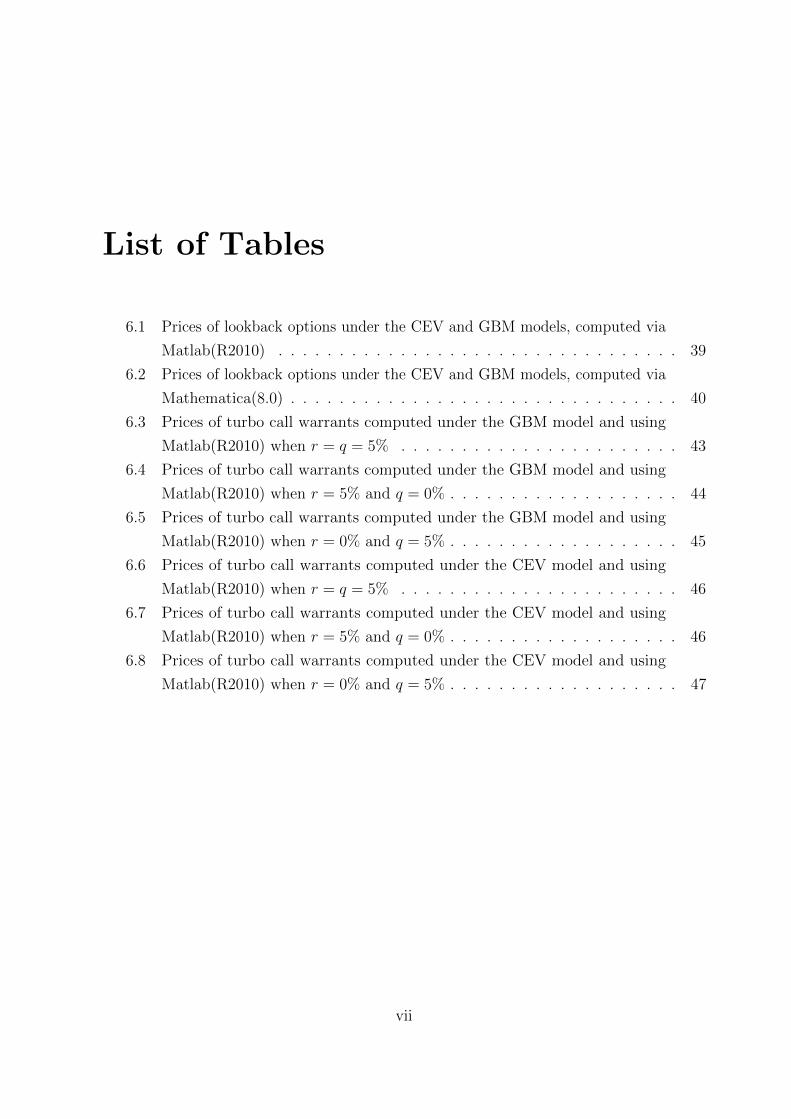
List of Tables
6.1 Prices of lookback options under the CEV and GBM models, computed via
Matlab(R2010) . . . . . . . . . . . . . . . . . . . . . . . . . . . . . . . . . 39
6.2 Prices of lookback options under the CEV and GBM models, computed via
Mathematica(8.0) . . . . . . . . . . . . . . . . . . . . . . . . . . . . . . . . 40
6.3 Prices of turbo call warrants computed under the GBM model and using
Matlab(R2010) when r = q = 5% . . . . . . . . . . . . . . . . . . . . . . . 43
6.4 Prices of turbo call warrants computed under the GBM model and using
Matlab(R2010) when r = 5% and q = 0% . . . . . . . . . . . . . . . . . . . 44
6.5 Prices of turbo call warrants computed under the GBM model and using
Matlab(R2010) when r = 0% and q = 5% . . . . . . . . . . . . . . . . . . . 45
6.6 Prices of turbo call warrants computed under the CEV model and using
Matlab(R2010) when r = q = 5% . . . . . . . . . . . . . . . . . . . . . . . 46
6.7 Prices of turbo call warrants computed under the CEV model and using
Matlab(R2010) when r = 5% and q = 0% . . . . . . . . . . . . . . . . . . . 46
6.8 Prices of turbo call warrants computed under the CEV model and using
Matlab(R2010) when r = 0% and q = 5% . . . . . . . . . . . . . . . . . . . 47
vii

List of Figures
6.1 Price of a floating strike lookback call under the CEV model when β = −1,
and for different values of n (number of terms used in the Euler method),
using Matlab(R2010) and Mathematica(8.0). . . . . . . . . . . . . . . . . . 41
viii
Chapter 1
Introduction
A turbo call (put) warrant is a contract which payoff is the same that the standard
call (put) option if a prespecified barrier has not been hit by the underlying asset price
before maturity. If the underlying asset price hits the barrier a rebate is paid. For turbo
call warrants the rebate is the difference between the lowest recorded stock-price during a
prespecified period after the barrier is hit and the strike price, and for turbo put warrants
the rebate is calculated as the difference between the strike price and the largest recorded
stock-price during a prespecified period after the barrier is hit.
Then turbo warrants are special types of barrier options because the rebate is calculated
as another exotic option. They first appeared in Germany at the end of 2001. Back then,
these contracts were only standard knock-out barrier options with the name ‘‘warrant’’.
The market segment for turbo warrants has had a big evolution since its introduction.
On February 2005, Societe Generale listed the first 40 turbo warrants on the Nordic
Derivatives Exchange. In Asia, the Hong Kong Exchange and Clearing Limited introduced
the callable bull/bear contracts, which are essentially turbo warrants.
Since then, there are some authors that studied these contracts under several models.
Eriksson (2006) derived closed-form solutions for the price of turbo warrants when the
underlying asset follows a lognormal process. Eriksson and Persson (2006) compared two
different methods to price numerically the turbo warrants offered by the Societe Generale:
Monte Carlo and finite difference methods. The valuation of turbo warrants under the
Constant Elasticity of Variance (CEV) model was implemented by Wong and Chan (2008).
These authors also consider a fast mean-reverting stochastic volatility process and two
time-scale volatility models. Further, Wong and Lau (2008) obtained analytical solutions
for turbo warrants under the double exponential jump diffusion model in terms of Laplace
transforms.
The price of turbo warrants can be obtained trough the valuation of barrier and
1
lookback options. Barrier options are probably the oldest path-dependent options. The
payoff of these options depends on the path of the underlying asset’s price. A barrier
option can become worthless or come into existence if the underlying asset price reaches
a certain level during a certain period of time. Snyder (1969) describes down-and-out
options as ‘‘limited risk special options’’. The lognormal assumption was covered by several
authors. The first pricing solution for down-and-out calls under the Black and Scholes
(1973) model1 were derived by Merton (1973), and geometric Brownian motion assumption
instituted the first step to the development of further studies on the pricing of barrier
options. Rubinstein and Reiner (1991), Benson and Daniel (1991) and Hudson (1991)
extended the analysis made by Merton (1973) for all eight types of single-barrier options2.
Still under the usual, a binomial method for barrier options was studied by Boyle and
Lau (1994). Kunitomo and Ikeda (1992) covered the valuation of double barrier options
expressing the probability density as a sum of normal density functions. Expressions
for the Laplace transform of a double barrier option price were derived by Geman and
Yor (1996). Pelsser (2000) derived analytical solutions to price double barriers using
a contour integration method. Further, Schroder (2000) derived the pricing formulas
of Kunitomo and Ikeda (1992) inverting the Laplace transforms derived in Geman and
Yor (1996). Based upon the Fourier series expansion, Lo and Hui (2007) proposed an
approach for computing accurate estimates of Black-Scholes double barrier option prices
with time-dependent parameters.
Although the Black and Scholes (1973) model revolutionized the financial markets, its
underlying assumptions are not observed in the market. The Black and Scholes (1973)
model assumes that the underlying asset price follows a lognormal distribution and its
volatility is constant, but the market shows that this is not true. For example, Schmalensee
and Trippi (1978) find a strong negative relationship between the stock prices changes
and changes in implied volatility. Jackwerth and Rubinstein (2001) show that the usual
geometric Brownian motion is unable to accommodate the negative skewness and the
high kurtosis that are usually implicit in empirical asset return distributions. The inverse
relation between the implied volatility and the strike price, known as volatility smile (see
Dennis and Mayhew, 2002), is not captured by the Black and Scholes (1973) model, and
therefore new models were studied.
The Constant Elasticity of Variance (CEV) model, which was developed by Cox (1975),
is one model that is consistent with the existence of a negative correlation between stock
returns and realized volatility, known as leverage effect (see Bekaert and Wu, 2000), and
1The Black and Scholes (1973) model assumes that the price of the underlying asset follows a geometricBrownian motion, and as a consequence the future underlying asset possesses a lognormal distribution.
2Up-and-out call or put, down-and-out call or put, up-and-in call or put and down-and-in call or put.
2
with the volatility smile (see Dennis and Mayhew, 2002). The pricing of barrier options
under the CEV model is done by various authors. Boyle and Tian (1999) used a trinomial
lattice to price single and double barrier options under this model. Davydov and Linetsky
(2001) derived analytical formulae for the prices of double barriers and lookback options
under the CEV model. Later, Davydov and Linetsky (2003) developed eigenfunctions
expansions for single and double barrier options, which were used to invert the Laplace
transforms of these contracts derived in Davydov and Linetsky (2001). Further, Lo et al.
(2009) derived the analytical kernels of the pricing formulae of the CEV knockout options
with time-dependent parameters for a parametric class of moving barriers.
Other models were used to price the barrier options. Under the Heston (1993) model,
Lipton (2001) and Faulhaber (2002) propose two different methods to price continuously
monitored double barrier options: the method of images and the eigenfunction expansion
approach. However, they have to assume two unrealistic assumption: a zero drift for the
underlying Ito process and the absence of correlation between the asset return and its
volatility. Still considering the Heston (1993) model, Griebsch and Wystup (2008) priced
discretely monitored barrier options through a multidimensional numerical integration
approach, avoiding the previous two assumptions described. Kuan and Webber (2003)
price single- and double-barrier options using the knowledge of the first passage time
density of the underlying asset price to the barrier level(s) under the geometric Brownian
motion assumption and one-factor interest rate models. However, the approach of Kuan
and Webber (2003) is the least efficient of the approaches under the lognormal assumption
(see Nunes and Dias, 2011). Under a one-dimensional diffusion process, Mijatovic (2010)
decomposed the price of double barrier options into a sum of integrals (along the time-
dependent barriers) of the option’s deltas. Finally, Nunes and Dias (2011) also decompose
the double barrier option price into a sum of integrals but over the first passage time
distributions of the (time-dependent) barriers. This last approach is based on a more
general multifactor and Markovian financial model, provides efficient pricing solutions, and
it is able to accommodate stochastic volatility, stochastic interest rates and endogenous
bankruptcy.
As a barrier option, a lookback option is also a path-dependent option. Its payoff
depends on the maximum or minimum stock price reached during the life of the option.
Lookback options were first studied by Goldman, Sosin and Shepp (1979a) and Goldman,
Sosin and Gatto (1979b) who derive closed-form pricing formulas under the lognormal
assumption. These analytical pricing formulas are re-derived and extended by Conze and
Viswanathan (1991). Babbs (2000) proposes a binomial model for floating strike lookback
options under the Black-Scholes assumptions. Using the arbitrage arguments of the Cox
3
et al. (1979) model, Cheuk and Vorst (1997) develope a binomial model for these options.
Further, Bermin (2000) shows how Malliavin calculus can be used to derive the hedging
strategy for any kind of path-dependent options, and in particular for lookback options.
Like in barrier options, the pricing of lookback options under the CEV model is done by
Boyle and Tian (1999) and Davydov and Linetsky (2001, 2003). Linetsky (2004) gives an
analytical characterization of lookback option prices in terms of spectral expansions, in
particular, under the CEV diffusion. Finally, Xu and Kwok (2005) derive general integral
price formulas for lookback option models using partial differential equation techniques.
The work developed in this thesis is based on the paper of Wong and Chan (2008)
and investigates the pricing of turbo warrants under the Black-Scholes and the CEV
models. To compute the price of turbo warrants, we follow the results of Davydov and
Linetsky (2001) for barrier and lookback options, including the proof of the results for the
lookback contracts. Thus, we use the Abate and Whitt (1995) algorithm in Matlab and
Mathematica to compute the necessary Laplace Transforms.
This thesis is organized as follow: In Chapter 2 we define the different types of lookback
options and their terminal payoffs. The value of a lookback option before maturity is
derived under a general one-dimensional diffusion process. The same analysis is done in
Chapter 3 but for turbo warrants. In Chapter 4, the Black-Scholes model is introduced and
its underlying assumptions are described. The formulae to compute the price of lookback
options and turbo warrants is derived in two different ways: using the formulae of Zhang
(1998) and using the formulas derived from the previous chapters 2 and 3. The price of
lookback options and turbo warrants under the CEV model is explained in Chapter 5
and the CEV model is described. In Chapter 6, we present numeric results for lookback
options and turbo warrants. The conclusions of this work are presented in Chapter 7.
4
Chapter 2
Lookback Options
European lookback options are exotic options whose terminal payoff depends on the
maximum or on the minimum attained by the underlying asset price during the life of
the option. There are two types of lookback options: floating and fixed strike lookback
options.
The option’s strike price of a floating strike lookback option is determined at maturity.
A floating strike lookback call gives the option holder the right to buy at the lowest price
recorded during the option’s life and a floating strike lookback put gives the holder the
right to sell at the highest price recorded during the option’s life.
A fixed strike lookback option has a prespecified strike price. The payoff of a fixed
strike call option is the maximum difference between the underlying asset’s highest price
(recorded during the option’s life) and the strike or zero, whichever is greater. The payoff
of a fixed strike put option is the maximum difference between the strike and underlying
asset’s lowest price (recorded during the option’s life) or zero, whichever is greater.
In next definitions, ST denotes the asset price at option’s maturity T , while m0,T and
M0,T denote the minimum and maximum asset prices recorded during the option’s life,
respectively.
Definition 1. The time-T value of a floating strike lookback call option on the asset S,
with a unit contract size, inception at time 0 and expiry date at time T (> 0) is:
LCfl(T ;ST ,m0,T , T ) = ST −m0,T . (2.1)
Definition 2. The time-T value of a floating strike lookback put option on the asset S,
with a unit contract size, inception at time 0 and expiry date at time T (> 0) is:
LPfl(T ;ST ,M0,T , T ) = M0,T − ST . (2.2)
5

Definition 3. The time-T value of a fixed strike lookback call option on the asset S, with
a unit contract size,a strike price equal to K, inception at time 0 and expiry date at time
T (> 0) is:
LCfx(T ;ST , K,M0,T , T ) = (M0,T −K)+ . (2.3)
Definition 4. The time-T value of a fixed strike lookback put option on the asset S, with
a unit contract size,a strike price equal to K, inception at time 0 and expiry date at time
T (> 0) is:
LPfx(T ;ST , K,m0,T , T ) = (K −m0,T )+ . (2.4)
Throughout this thesis, St will denote the stock-price process at time t. We take
an equivalent martingale measure (risk-neutral probability measure) Q as given (see
Duffie, 1996, p.923-924). Under Q, we suppose that the asset price is a time-homogeneous,
nonnegative diffusion process solving the stochastic differential equation
dSt = µSt + σ(St)dWt, t ≥ 0, S0 = S > 0, (2.5)
where Wt : t ≥ 0 is a standard Brownian motion defined on a filtered probability space
(Ω,F , Ftt≥0,Q), µ is a constant (µ = r − q, where r ≥ 0 and q ≥ 0 are the constant
risk-free interest rate and the constant dividend yield, respectively), and σ = σ(St) is a
given local volatility function, which is assumed to be continuous and strictly positive for
all S ∈ (0,∞). Note that σ = σ(St) is independent of t.
Using equations (2.1)-(2.4) and risk-neutral valuation, the time-t (0 ≤ t < T ) values of
the floating strike lookback call, the floating strike lookback put, the fixed strike lookback
call and the fixed strike lookback put are given by:
LCfl(t;St,m0,t, T ) = e−rτEQ [ST −m0,T |Ft] , (2.6)
LPfl(t;St,M0,t, T ) = e−rτEQ [M0,T − ST |Ft] , (2.7)
LCfx(t;St, K,M0,t, T ) = e−rτEQ[(M0,T −K)+|Ft
], (2.8)
LPfx(t;St, K,m0,T , T ) = e−rτEQ[(K −m0,T )+|Ft
], (2.9)
where all contracts are initiated at time zero, m0,t and M0,t are the minimum and maximum
asset prices recorded until date t, St is the current underlying asset price at time t, and
τ = T − t is the time remaining to expiration.
To obtain closed-form solutions for the prices of lookback options we need to find the
probability distributions of the maximum and minimum asset prices. The next result gives
6
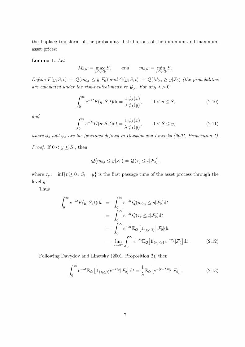
the Laplace transform of the probability distributions of the minimum and maximum
asset prices:
Lemma 1. Let
Ma,b := maxa≤u≤b
Su and ma,b := mina≤u≤b
Su
Define F (y;S, t) := Q(m0,t ≤ y|F0) and G(y;S, t) := Q(M0,t ≥ y|F0) (the probabilities
are calculated under the risk-neutral measure Q). For any λ > 0∫ ∞0
e−λtF (y;S, t)dt =1
λ
φλ(x)
φλ(y), 0 < y ≤ S, (2.10)
and ∫ ∞0
e−λtG(y;S, t)dt =1
λ
ψλ(x)
ψλ(y), 0 < S ≤ y, (2.11)
where φλ and ψλ are the functions defined in Davydov and Linetsky (2001, Proposition 1).
Proof. If 0 < y ≤ S , then
Q(m0,t ≤ y|F0
)= Q
(τy ≤ t|F0
),
where τy := inft ≥ 0 : St = y is the first passage time of the asset process through the
level y.
Thus ∫ ∞0
e−λtF (y;S, t)dt =
∫ ∞0
e−λtQ(m0,t ≤ y|F0)dt
=
∫ ∞0
e−λtQ(τy ≤ t|F0)dt
=
∫ ∞0
e−λtEQ[11τy≤t
∣∣F0]dt
= limr→0+
∫ ∞0
e−λtEQ[11τy≤te
−rτy |F0
]dt . (2.12)
Following Davydov and Linetsky (2001, Proposition 2), then∫ ∞0
e−λtEQ[11τy≤te
−rτy |F0
]dt =
1
λEQ[e−(r+λ)τy |F0
]. (2.13)
7
Hence, equations (2.12) and (2.13) yield
∫ ∞0
e−λtF (y;S, t)dt = limr→0+
(1
λEQ[e−(r+λ)τy |F0
])=
1
λEQ[e−λτy |F0
]=
1
λEQ[e−λτy11τy<∞|F0
], (2.14)
where the last equality arises because EQ[e−λτy
]= 0 when τy =∞.
Using Davydov and Linetsky (2001, Equation 2), it is well known that
EQ[e−λτy11τy<∞|F0
]=φλ(S)
φλ(y), S ≥ y . (2.15)
Therefore, combining equations (2.14) and (2.15),∫ ∞0
e−λtF (y;S, t)dt =1
λ
φλ(S)
φλ(y), S ≥ y .
If 0 < S ≤ y and assuming that the barrier at zero is an absorbing barrier, then
Q(M0,t ≥ y|F0) = Q(τy ≤ t ∧ τy < τ0) ,
where τa := inft ≥ 0 : St = a , a ∈ 0, y .
Thus, if τy < τ0, then∫ ∞0
e−λtG(y;S, t)dt =
∫ ∞0
e−λtQ(M0,t ≥ y|F0)dt
=
∫ ∞0
e−λtQ(τy ≤ t|F0)dt
=
∫ ∞0
e−λtEQ[11τy≤t|F0
]dt
= limr→0+
∫ ∞0
e−λtEQ[11τy≤te
−rτy |F0
]dt .
8
Using again equation (2.13), then
∫ ∞0
e−λtG(y;S, t)dt = limr→0+
(1
λEQ[e−(r+λ)τy |F0
])=
1
λEQ[e−λτy |F0
]=
1
λEQ[e−λτy11τy<τ0|F0
]+
1
λEQ[e−λτy11τy≥τ0|F0
]=
1
λEQ[e−λτy11τy<τ0|F0
], (2.16)
where the last equality arises because τy ≥ τ0 = ∅, since τ0 represents the default time
of the asset.
Using again Davydov and Linetsky (2001, Equation 2), it follows that
EQ[e−λτy11τy<τ0|F0
]=ψλ(S)
ψλ(y), S ≤ y . (2.17)
Hence, equations (2.16) and (2.17) can be combined into∫ ∞0
e−λtG(y;S, t)dt =1
λ
ψλ(S)
ψλ(y), S ≤ y .
The probability distributions of the minimum and maximum asset prices are recovered
by inverting the Laplace transforms. The next proposition provides closed-form solutions
to compute the lookback prices in terms of these probabilities.
Proposition 1. The prices of the floating strike lookback call, the floating strike lookback
put, the fixed strike lookback call and the fixed strike lookback put at some time 0 ≤ t < T
during the option’s life are:
LCfl(t;St,m0,t, T ) = e−qτSt − e−rτm0,t + e−rτ∫ m0,t
0
F (y;St, τ)dy (2.18)
LPfl(t;St,M0,t, T ) = e−rτM0,t − e−qτSt + e−rτ∫ ∞M0,t
G(y;St, τ)dy (2.19)
LCfx(t;St, K,M0,t, T ) =
e−rτ∫∞KG(y;St, τ)dy ⇐M0,t ≤ K
e−rτM0,t − e−rτK + e−rτ∫∞M0,t
G(y;St, τ)dy ⇐M0,t > K
(2.20)
9

LPfx(t;St, K,m0,t, T ) =
e−rτ∫ K
0F (y;St, τ)dy ⇐ m0,t ≥ K
e−rτK − e−rτm0,t + e−rτ∫ m0,t
0F (y;St, τ)dy ⇐ m0,t < K
(2.21)
where all contracts are initiated at time zero, m0,t andM0,t are the minimum and maximum
prices recorded until date t, St is the current underlying asset price at time t, τ = T − t isthe time remaining to expiration and F (y;St, τ) and G(y;St, τ) are defined in Lemma 1.
Proof. See Appendix A.
Finally, to compute the price of a lookback option it is only necessary to invert the
Laplace transforms offered by equations (2.10) and (2.11), and to plug-in the results into
equations (2.18) - (2.21), according to the lookback contract we need to value.
10

Chapter 3
Turbo Warrants
Let St be the underlying asset price at time t. The turbo warrants that we consider
can have the following payoffs:
• A turbo call warrant pays the option holder (ST −K)+ at maturity T , where K is
the option’s strike price, if a prespecified barrier H ≥ K has not been hit by St at
any time before the maturity. If St hits the barrier the contract is void and a new
contract starts. This new contract is a call option on the minimum process of St,
with the same strike price K, and time to maturity T0.
• A turbo put warrant pays (K−ST )+ at maturity T , where K is the option’s strike
price, if a prespecified barrier H ≤ K has not been hit by St at any time before the
maturity. If St hits the barrier the contract is void and a new contract starts. This
new contract is a put option on the maximum process of St, with the same strike
price K, and time to maturity T0.
From definition above, we can write the value of a turbo call warrant as a sum of two
parts. The first part is a down-and-out call option (DOC) with a zero rebate, and the
second part is a down and in lookback option (DIL).
Define
τH := inft ≥ 0 : St ≤ H and mτH ,τH+T0 := minτH≤u≤τH+T0
Su .
By risk-neutral valuation, the value of the DOC and DIL, respectively, is given at
time t < τH by the following expressions
DOC(t, S) = e−r(T−t)EQ[(ST −K)+11τH>T|Ft
], (3.1)
and
DIL(t, S, T0) = EQ[e−r(τH+T0−t)(mτH ,τH+T0 −K)+11τH≤T|Ft
]. (3.2)
11
The price of the turbo call at time t < τH is given by
TC(t, S) = DOC(t, S) +DIL(t, S, T0) . (3.3)
The next result gives the price of the turbo call, in closed-form.
Proposition 2. At t < τH , the model-free representation of the turbo call warrant price
is given by
TC(t, S) = DOC(t, S) + EQ[e−r(τH−t)11τH≤TLB(τH , SτH , T0)|Ft
], (3.4)
where
LB(τH , SτH , T0) = LCfl(τH ;SτH ,minSτH , K, τH + T0)− LCfl(τH ;SτH , SτH , τH + T0).
(3.5)
Proof. First, we can write (mτH ,τH+T0 −K)+ in other form. So,
(mτH ,τH+T0 −K)+
=
mτH ,τH+T0 −K ⇐ mτH ,τH+T0 > K
0 ⇐ mτH ,τH+T0 ≤ K
=
(SτH+T0 −K)− (SτH+T0 −mτH ,τH+T0) ⇐ mτH ,τH+T0 > K
(SτH+T0 −mτH ,τH+T0)− (SτH+T0 −mτH ,τH+T0) ⇐ mτH ,τH+T0 ≤ K
= SτH+T0 −K + (K −mτH ,τH+T0)11mτH,τH+T0≤K − (SτH+T0 −mτH ,τH+T0)
= SτH+T0 −K + (K −mτH ,τH+T0)+ − (SτH+T0 −mτH ,τH+T0) . (3.6)
Assuming that t < τH , using the tower expectation formula and equation (3.2), we get
DIL(t, S, T0) = EQe−r(τH−t)11τH≤TLB(τH , SτH , T0)|Ft
, (3.7)
where
LB(τH , SτH , T0) := EQ[e−rT0(mτH ,τH+T0 −K)+|FτH
]. (3.8)
12

Using equation (3.6),
LB(τH , SτH , T0) = EQ[e−rT0(mτH ,τH+T0 −K)+|FτH
]= EQ
[e−rT0
SτH+T0 −K + (K −mτH ,τH+T0)
+
−(SτH+T0 −mτH ,τH+T0)|FτH
]= e−rT0EQ
[SτH+T0
∣∣FτH]− e−rT0K + e−rT0EQ[(K −mτH ,τH+T0)
+∣∣FτH]
−e−rT0EQ[SτH+T0 −mτH ,τH+T0
∣∣FτH]= e−rT0SτHe
(r−q)T0 − e−rT0K + e−rT0EQ[(K −mτH ,τH+T0)
+∣∣FτH]
−e−rT0EQ[SτH+T0 −mτH ,τH+T0
∣∣FτH] . (3.9)
The last equation was obtained due to the fact that EQ(ST |Ft) = Ste(r−q)(T−t).
Comparing equation (2.6) with e−rT0EQ[SτH+T0 −mτH ,τH+T0
∣∣FτH], we conclude that
this expression is simply the value at time τH of a floating strike lookback call, on asset S,
inception at time τH and expiry date at time τH + T0. Thus,
e−rT0EQ[SτH+T0 −mτH ,τH+T0
∣∣FτH] = LCfl(τH ;SτH ,mτH ,τH , τH + T0) .
Notice that mτH ,τH = minτH≤u≤τH Su = SτH . Therefore,
e−rT0EQ[SτH+T0 −mτH ,τH+T0
∣∣FτH] = LCfl(τH ;SτH , SτH , τH + T0) . (3.10)
Comparing expression e−rT0EQ[(K −mτH ,τH+T0)
+∣∣FτH] with equation (2.9), we con-
clude that this expression is the value at time τH of a fixed strike lookback put, on asset
S, strike price equal to K, inception at time τH and expiry date at time τH + T0. Thus,
e−rT0EQ[(K −mτH ,τH+T0)
+∣∣FτH] = LPfx(τH ;SτH , K,mτH ,τH , τH + T0)
= LPfx(τH ;SτH , K, SτH , τH + T0) . (3.11)
Using equation (2.21), the last equation becomes
e−rT0EQ[(K −mτH ,τH+T0)
+∣∣FτH]
=
e−rT0
∫ K0F (y;SτH , T0)dy ⇐ SτH ≥ K
e−rT0K − e−rT0SτH + e−rT0∫ SτH
0F (y;SτH , T0)dy ⇐ SτH < K
, (3.12)
where F (y;SτH , T0) = Q(mτH ,τH+T0 ≤ y|FτH ).
13

Combining equations (3.9), (3.10) and (3.12), we get
LB(τH , SτH , T0)
=
e−qT0SτH − e−rT0K + e−rT0∫ K
0F (y;SτH , T0)dy
−LCfl(τH ;SτH , SτH , τH + T0) ⇐ SτH ≥ K
e−qT0SτH − e−rT0K + e−rT0K − e−rT0SτH+e−rT0
∫ SτH0
F (y;SτH , T0)dy − LCfl(τH ;SτH , SτH , τH + T0) ⇐ SτH < K
=
e−qT0SτH − e−rT0K + e−rT0∫ K
0F (y;SτH , T0)dy
−LCfl(τH ;SτH , SτH , τH + T0) ⇐ SτH ≥ K
e−qT0SτH − e−rT0SτH + e−rT0∫ SτH
0F (y;SτH , T0)dy
−LCfl(τH ;SτH , SτH , τH + T0) ⇐ SτH < K
= e−qT0SτH − e−rT0 minSτH , K+ e−rT0∫ minSτH ,K
0
F (y;SτH , T0)dy
−LCfl(τH ;SτH , SτH , τH + T0) .
Using equation (2.18), the last equation becomes
LB(τH , SτH , T0) = LCfl(τH ;SτH ,minSτH , K, τH + T0)− LCfl(τH ;SτH , SτH , τH + T0) .
(3.13)
Equations (3.3), (3.7) and (3.13) yield equation (3.4).
If the underlying asset price follows a stochastic process of continuous sample paths,
then we have SτH = H. So the next corollary simplifies the price of a turbo call warrant
under this condition.
Corollary 1. If the asset price follows a continuous diffusion process, then, at t < τH ,
the turbo call price reads
TC(t, S) = DOC(t, S) + EQ[e−r(τH−t)11τH≤TLB(τH , H, T0)|Ft
], (3.14)
where LB(τH , H, T0) is obtained by replacing SτH for H in equation (3.5).
Proof. Equation (3.14) follows from Proposition 2 because if the asset price follows a
continuous diffusion process, then SτH = H.
Corollary 1 can be applied to local volatility and stochastic volatility models. If the
asset price is a diffusion process like in equation (2.5) then the following result holds. Note
14

that the Black-Scholes and the CEV models are special cases of the time-independent
local volatility model.
Corollary 2. If the asset price follows a time-independent local volatility model, then, at
t < τH , the turbo call price reads
TC(t, S) = DOC(t, S) + LB(0, H, T0)EQ[e−r(τH−t)11τH≤T|Ft
], (3.15)
where
LB(0, H, T0) = LCfl(0;H,K, T0)− LCfl(0;H,H, T0) . (3.16)
Proof. Replacing SτH for H in equation (3.13), we get
LB(τH , H, T0) = LCfl(τH ;H,minH,K, τH + T0)− LCfl(τH ;H,H, τH + T0) .
According to the definition of a turbo warrant call, we know that H ≥ K. So, the last
equation becomes
LB(τH , H, T0) = LCfl(τH ;H,K, τH + T0)− LCfl(τH ;H,H, τH + T0). (3.17)
Using equation (2.18), the last equation can be written as
LB(τH , H, T0) = e−qT0H − e−rT0K + e−rT0∫ K
0
F (y;H,T0)dy
−e−qT0H + e−rT0H − e−rT0∫ H
0
F (y;H,T0)dy .
Simplifying, the last equation becomes
LB(τH , H, T0) = (H −K)e−rT0 − e−rT0∫ H
K
F (y;H,T0)dy . (3.18)
The function F (y;H,T0) is equal to Q(mτH ,τH+T0 ≤ y|FτH ), but can also be written as
Q(m0,T0 ≤ y|F0) given by Markovian nature of the pricing model under analysis, which
means that the only relevant information on the future of the process is its present value,
and its past is irrelevant. Therefore, equation (3.18) can be written as
LB(τH , H, T0) = (H −K)e−rT0 − e−rT0∫ H
K
Q(m0,T0 ≤ y|F0)dy ,
i.e.,
LB(τH , H, T0) = LB(0, H, T0). (3.19)
15

which is independent of τH . Replacing τH by 0 in equation (3.17) we get equation (3.16).
Combing equations (3.14) and (3.19), the turbo call price reads
TC(t, S) = DOC(t, S) + EQ[e−r(τH−t)11τH≤TLB(0, H, T0)|Ft
]= DOC(t, S) + LB(0, H, T0)EQ
[e−r(τH−t)11τH≤t|Ft
].
The last equation arises because LB(0, H, T0) is Ft - measurable.
To compute the price of the turbo warrant under a time-independent local volatility
model, we need to compute the DOC option, as well as the LB part and the expectation
EQ[e−r(τH−t)11τH≤t|Ft]. If the asset price is a diffusion process solving the stochastic
differential equation (2.5) and respecting all the assumptions that were referred in Chapter
2, then we can follow Davydov and Linetsky (2001) to compute both parts:
• The DOC component in the turbo call warrant is given by equation (3.1). Let
τ(H,U) := inft ≥ 0 : St /∈ (H,U). Then limU→∞ τ(H,U) = τH . Let
DBKO(t, S) = e−r(T−t)EQ[11τ(H,U)>T(ST −K)+|Ft] (3.20)
be the value of a double barrier knock out option at time t. To compute the DOC
option we need to take the limit of DBKO as U approaches infinity.
Davydov and Linetsky (2001) have obtained a closed-form solution for double barrier
options under a general one-dimensional diffusion, when the strike price is between
the lower and the upper barriers. To compute the DOC component in the turbo call
we have to modify their solution because the strike price is less than the downside
barrier and we have to take the limit U → ∞. Next result presents the expected
value of the terminal payoff of a double knock out option in terms of its Laplace
Transform, when the strike price is less than the downside barrier.
Proposition 3. The Laplace Transform of the expected value of the terminal payoff
of a double knock out option, when the strike price (K) is less than the downside
barrier (L) is given by:∫ ∞0
e−λTEQ[11τ(L,U)>T(ST −K)+]dT
=1
ωλ∆λ(L,U)
(∆λ(L, S)
[ψλ(U)Jλ(K,S, U)− φλ(U)Iλ(K,S, U)
]+∆λ(S, U)
[φλ(L)Iλ(K,L, S)− ψλ(L)Jλ(K,L, S)
]), (3.21)
16

where ωλ is defined in Davydov and Linetsky (2001, Equation 13) through the ODE
φλ(S)dψλdS
(S)− ψλ(S)dφλdS
(S) = s(S)wλ , (3.22)
and
∆λ(A,B) := φλ(A)ψλ(B)− ψλ(A)φλ(B) . (3.23)
Moreover,
Iλ(K,A,B) =
∫ B
A
(Y −K)ψλ(Y )m(Y )dY, (3.24)
and
Jλ(K,A,B) =
∫ B
A
(Y −K)φλ(Y )m(Y )dY, (3.25)
where m(Y ) is the speed density of the diffusion (2.5) that is defined by
m(Y ) :=2
σ2(Y )Y 2s(Y ). (3.26)
In equations (3.22) and (3.26), s(S) is the scale density of diffusion (2.5), which is
defined as
s(S) := exp
−∫
2µ
σ2(S)SdS
. (3.27)
Proof. See Appendix B.
Therefore, to compute the DOC option we need to take the limit U →∞ in equation
(3.20) and use the boundary properties of the functions φλ and ψλ defined in Davydov
and Linetsky (2001, Proposition 1). The useful boundary properties are
limS→∞
ψλ(S) = +∞ limS→∞
φλ(S) = 0 . (3.28)
Under certain conditions, we can get a simple expression of the DOC option. Next
result provides this expression.
Proposition 4. If
limU→∞
Jλ(K,S, U) < +∞ and limU→∞
Iλ(K,S, U) < +∞ , (3.29)
17
or if
limU→∞
Jλ(K,S, U) < +∞ and limU→∞
φλ(U)
ψλ(U)Iλ(K,S, U) = 0 (3.30)
then the Laplace transform of the expected value of the terminal payoff of a down-
and-out call option, when the strike price (K) is less than the downside barrier (L),
is given by ∫ ∞0
e−λTEQ[11τL>T(ST −K)+]dT
=1
ωλφλ(L)
(∆λ(L, S) lim
U→∞
(Jλ(K,S, U)
)+ φλ(S)
[φλ(L)Iλ(K,L, S)
−ψλ(L)Jλ(K,L, S)]), (3.31)
where τL := inft ≥ 0 : St = L.
Proof. Using equations (3.21) and (3.23), we get∫ ∞0
e−λTEQ[11τL>T(ST −K)+]dT
= limU→∞
1
ωλ(φλ(L)ψλ(U)− ψλ(L)φλ(U))(∆λ(L, S)
[ψλ(U)Jλ(K,S, U)− φλ(U)Iλ(K,S, U)
]+(φλ(S)ψλ(U)− ψλ(S)φλ(U)
)[φλ(L)Iλ(K,L, S)− ψλ(L)Jλ(K,L, S)
])= lim
U→∞
1
ωλ(φλ(L)− ψλ(L)φλ(U) 1
ψλ(U)
)(∆λ(L, S)
[Jλ(K,S, U)− φλ(U)
1
ψλ(U)Iλ(K,S, U)
]+
(φλ(S)− ψλ(S)φλ(U)
1
ψλ(U)
)[φλ(L)Iλ(K,L, S)− ψλ(L)Jλ(K,L, S)
])=
1
ωλφλ(L)
(∆λ(L, S) lim
U→∞
(Jλ(K,S, U)
)+ φλ(S)
[φλ(L)Iλ(K,L, S)
−ψλ(L)Jλ(K,L, S)]).
Therefore, to find the price of the DOC option we need to invert the Laplace
transform of equation (3.31) and multiply the result by e−r(T−t).
18
• The LB(0, H, T0) formula can be obtained using the following equation
LB(0, H, T0) = (H −K)e−rT0 − e−rT0∫ H
K
F (y;H,T0)dy , (3.32)
where F (y;H,T0) is obtained by inverting the Laplace transform of equation (2.10).
• The expectation EQ[e−r(τH−t)11τH≤T|Ft] can be computed using two results of
Davydov and Linetsky (2001). Let
DR(t, S) = EQ[e−r(τH−t)11τH≤T|Ft] . (3.33)
Using the fact that the asset price is a time-homogeneous diffusion process, then we
can write this in another way:
DR(t, S) = EQ[e−rτH11τH≤T|F0
]Using the result of Davydov and Linetsky (2001, Proposition 2),∫ ∞
0
e−λtDR(t, S)dt =1
λEQ[e−(r+λ)τH |F0
]=
1
λEQ[e−(r+λ)τH11τH<∞|F0
], (3.34)
because EQ[e−(r+λ)τH
]= 0 when τH = ∞. Using Davydov and Linetsky (2001,
Equation 2), we get
EQ[e−(r+λ)τH11τH<∞|F0
]=φr+λ(S)
φr+λ(H). (3.35)
Combining equations (3.34) and (3.35), we get the Laplace transform of DR:∫ ∞0
e−λtDR(t, S)dt =1
λ
φr+λ(S)
φr+λ(H). (3.36)
Therefore, the DR value is obtained by inverting the Laplace transform of the last
equation.
19

Chapter 4
GBM Model
In 1973, Black and Scholes (1973) and Merton (1973) published their papers on the
theory of option pricing. They developed the Black-Scholes model, which has had a huge
influence on the development of option and derivative industries.
The Black-Scholes risk-neutral formulation of the option pricing theory is attractive
due to the fact that the pricing formula of a derivative is a function of directly observable
parameters (with exception of the volatility parameter). The assumptions of this model
are:
i) The underlying asset price follows a geometric Brownian (GBM) motion:
dSt = rStdt+ σStdWQt ,
with r and σ constant.
ii) The short selling of securities with full use of proceeds is permitted.
iii) There are no transactions costs or taxes.
iv) The assets are perfectly divisible.
v) The asset pays no dividend.
vi) There are no riskless arbitrage opportunities.
vii) Trading takes place continuously in time.
viii) The risk-free rate of interest, r, is constant and the same for all maturities.
The Black and Scholes (1973) option pricing model can be extended to deal with
options on dividend-paying stocks:
dSt = µStdt+ σStdWQt , (4.1)
20

where Q is an equivalent martingale measure (risk-neutral probability measure). Under
Q, we suppose that the asset price is a time-homogeneous, nonnegative diffusion process;
WQt : t ≥ 0 is a standard Brownian motion defined on a filtered probability space
(Ω,F , Ftt≥0,Q) and µ is a constant (µ = r − q, where r ≥ 0 and q ≥ 0 are the constant
risk-free interest rate and the constant dividend yield, respectively). Under this model,
the stock return dStSt
in the small interval dt is normally distributed with mean µdt and
variance σ2dt.
Unfortunately, this model is not consistent with the empirical evidence, as explained
in Chapter 1. In the next chapter we will study the CEV model, wherein the prices are
closer to market quotes.
4.1 Lookback options under the GBM Model
We can compute the price of the lookback options under the Black-Scholes model in
two different ways: using equations (2.10) - (2.11) and (2.18) - (2.21), or using the pricing
formulae of Zhang (1998, p.341-352).
To compute the price of lookback options using equations (2.10) - (2.11) and (2.18) -
(2.21), functions ψλ and φλ can be replaced in equations (2.10) and (2.11) by closed-form
solutions. Functions ψλ and φλ are defined in Davydov and Linetsky (2001, equation 15):
ψλ = Sγ+ , (4.2)
and
φλ = Sγ− , (4.3)
where
γ± = −γ ±√γ2 +
2λ
σ2, (4.4)
with
γ =µ
σ2− 1
2. (4.5)
Using the pricing formulae of Zhang (1998, p. 346-352),1 the prices of the floating
strike lookback call, the floating strike lookback put, the fixed strike lookback call and the
1Equations (4.6)-(4.9) are different from Zhang (1998) when r = q, i.e. when the drift is zero. Theproof of these equations for the case r = q is given in Appendix C.
21

fixed strike lookback put at some time 0 ≤ t < T and during the option’s life are:
LCfl(t;St,m0,t, T )
=
Ste−qτΦ
[dbs1(St,m0,t)
]−m0,te
−rτΦ[dbs(St,m0,t)
]+St
δ
e−rτ
(Stm0,t
)−δΦ[dbs(m0,t, St)
]− e−qτΦ
[− dbs1(St,m0,t)
], ⇐ r 6= q
Ste−qτΦ
[dbs1(St,m0,t)
]−m0,te
−rτΦ[dbs(St,m0,t)
]+Ste
−rτσ√τf[− dbs1(St,m0,t)
]−Ste−rτ σ
2
2Φ[− dbs1(St,m0,t)
]2σ2 ln
(Stm0,t
)+ τ, ⇐ r = q
(4.6)
LPfl(t;St,M0,t, T )
=
M0,te−rτΦ
[− dbs(St,M0,t)
]− Ste−qτΦ
[− dbs1(St,M0,t)
]+St
δ
e−qτΦ
[dbs1(St,M0,t)
]− e−rτ
(StM0,t
)−δΦ[− dbs(M0,t, St)
], ⇐ r 6= q
M0,te−rτΦ
[− dbs(St,M0,t)
]− Ste−qτΦ
[− dbs1(St,M0,t)
]+Ste
−rτσ√τf[dbs1(St,M0,t)
]+Ste
−rτ σ2
2Φ[dbs1(St,M0,t)
]2σ2 ln
(StM0,t
)+ τ, ⇐ r = q
(4.7)
LCfx(t;St, K,M0,t, T )
=
e−rτ (M0,t −K)+ + Ste−qτΦ
[dbs1(St,maxM0,t, K)
]−maxM0,t, Ke−rτΦ
[dbs(St,maxM0,t, K)
]+St
δ
e−qτΦ
[dbs1(St,maxM0,t, K)
]−e−rτ
(St
maxM0,t,K
)−δΦ[− dbs(maxM0,t, K, St)
], ⇐ r 6= q
e−rτ (M0,t −K)+ + Ste−qτΦ
[dbs1(St,maxM0,t, K)
]−maxM0,t, Ke−rτΦ
[dbs(St,maxM0,t, K)
]+Ste
−rτσ√τf[dbs1(St,maxM0,t, K)
]+Ste
−rτ σ2
2Φ[dbs1(St,maxM0,t, K)
]2σ2 ln
(St
maxM0,t,K
)+ τ, ⇐ r = q
(4.8)
22
LPfx(t;St, K,m0,t, T )
=
e−rτ (K −m0,t)+ + minm0,t, Ke−rτΦ
[− dbs(St,minm0,t, K)
]−Ste−qτΦ
[− dbs1(St,minm0,t, K)
]+St
δ
− e−qτΦ
[− dbs1(St,minm0,t, K)
]+e−rτ
(St
minm0,t,K
)−δΦ[dbs(minm0,t, K, St)
], ⇐ r 6= q
e−rτ (K −m0,t)+ + minm0,t, Ke−rτΦ
[− dbs(St,minm0,t, K)
]−Ste−qτΦ
[− dbs1(St,minm0,t, K)
]+Ste
−rτσ√τf[− dbs1(St,minm0,t, K)
]−Ste−rτ σ
2
2Φ[− dbs1(St,minm0,t, K)
] 2σ2 ln
(St
minm0,t,K
)+ τ, ⇐ r = q
(4.9)
where Φ[.] is the normal cumulative distribution function, f [.] is the normal probability
density function,
dbs(Y,X) =ln(Y/X) + (r − q − σ2/2)τ
σ√τ
, (4.10)
dbs1(Y,X) = dbs(Y,X) + σ√τ , (4.11)
δ =2(r − q)σ2
, (4.12)
and where all contracts are initiated at time zero, m0,t and M0,t are the minimum and
maximum prices recorded until date t, St is the current underlying asset price at time t
and τ = T − t is the time remaining to expiration.
4.2 Turbo Warrants under the GBM Model
The explicit solution of turbo warrants under the Black-Scholes model can be obtained
by replacing functions ψλ and φλ given by equations (4.2) and (4.3), repectively, into
equations (3.31),2 (3.32) and (3.36). For the DOC component we have to find the
expression of speed density of diffusion (4.1) to compute in closed form the integrals (3.24)
and (3.25).
Then, the scale density is defined by (3.27). Replacing σ(S) for σ, the scale density
2See Proposition 5 in page 26 for the proof of conditions of Proposition 4.
23

becomes
s(S) = exp
− 2µ
σ2
∫1
SdS
= exp
ln(S−
2µ
σ2
)= S−
2µ
σ2 . (4.13)
Therefore, the speed density defined by equation (3.26) becomes
m(S) =2
σ2S2S−2µ
σ2
=2
σ2S2− 2µ
σ2
. (4.14)
Replacing the functions ψλ and φλ given by equations (4.2) and (4.3) and the speed
density in equation (4.14) in equation (3.22), the Wronskian of the functions ψλ and φλ
with respect of the scale density of equation (4.13) is given by
Sγ−Sγ+−1γ+ − Sγ+Sγ−−1γ− = S−2µ
σ2 ωλ
S−2γ−1
(2
√γ2 +
2λ
σ2
)= S−
2µ
σ2 ωλ . (4.15)
The last equation arises because γ± = −γ ±√γ2 + 2λ
σ2 . Using the fact that γ = µσ2 − 1
2,
equation (4.15) becomes
2S−2( µ
σ2− 1
2)−1
√γ2 +
2λ
σ2= S−
2µ
σ2 ωλ
2
√γ2 +
2λ
σ2= ωλ . (4.16)
The integrals Iλ and Jλ are defined in equations (3.24) and (3.25), respectively. Re-
placing the functions ψλ and φλ given by equations (4.2)-(4.3) and the speed density given
by equation (4.14) into equations (3.24) and (3.25), and using the definitions stated in
equations (4.4) and (4.5), these integrals become:
24

Iλ(K,A,B)
=
∫ B
A
(Y −K)Y γ+2
σ2Y 2− 2µ
σ2
dY
=2
σ2
(∫ B
A
Y γ+−1+ 2µ
σ2 dY −K∫ B
A
Y γ+−2+ 2µ
σ2 dY
)
=2
σ2
[Y γ++ 2µ
σ2
γ+ + 2µσ2
]BA
−K
[Y γ++ 2µ
σ2−1
γ+ + 2µσ2 − 1
]BA
=
2
σ2
Y
µ
σ2+ 1
2+√γ2+ 2λ
σ2
µσ2 + 1
2+√γ2 + 2λ
σ2
BA
−K
Yµ
σ2− 1
2+√γ2+ 2λ
σ2
µσ2 − 1
2+√γ2 + 2λ
σ2
BA
=
2
σ2
Y
1−(− µ
σ2+ 1
2−√γ2+ 2λ
σ2
)1−
(− µσ2 + 1
2−√γ2 + 2λ
σ2
)B
A
−K
Y−(− µ
σ2+ 1
2−√γ2+ 2λ
σ2
)−(− µσ2 + 1
2−√γ2 + 2λ
σ2
)B
A
=
2
σ2
[ Y 1−γ−
1− γ−
]BA
+K
[Y −γ−
γ−
]BA
(4.17)
Jλ(K,A,B)
=
∫ B
A
(Y −K)Y γ−2
σ2Y 2− 2µ
σ2
dY
=2
σ2
(∫ B
A
Y γ−−1+ 2µ
σ2 dY −K∫ B
A
Y γ−−2+ 2µ
σ2 dY
)
=2
σ2
[Y γ−+ 2µ
σ2
γ− + 2µσ2
]BA
−K
[Y γ−+ 2µ
σ2−1
γ− + 2µσ2 − 1
]BA
=
2
σ2
Y
µ
σ2+ 1
2−√γ2+ 2λ
σ2
µσ2 + 1
2−√γ2 + 2λ
σ2
BA
−K
Yµ
σ2− 1
2−√γ2+ 2λ
σ2
µσ2 − 1
2−√γ2 + 2λ
σ2
BA
=
2
σ2
Y
1−(− µ
σ2+ 1
2+√γ2+ 2λ
σ2
)1−
(− µ
σ2 + 12
+√γ2 + 2λ
σ2 )
BA
−K
Y−(− µ
σ2+ 1
2+√γ2+ 2λ
σ2
)−(− µ
σ2 + 12
+√γ2 + 2λ
σ2
)BA
=
2
σ2
[ Y 1−γ+
1− γ+
]BA
+K
[Y −γ+
γ+
]BA
. (4.18)
25
To apply the equation (3.31) we need to prove that the conditions in equation (3.30)
are true. Next proposition give us that proof and the closed-form for limU→∞ Jλ(K,S, U).
Proposition 5. Under GBM assumptions, for any S > 0 and for λ > 0 large such that
1 + γ −√γ2 +
2λ
σ2< 0, (4.19)
we have
limU→∞
φλ(U)
ψλ(U)Iλ(K,S, U) = 0 , (4.20)
and
limU→∞
Jλ(K,S, U) = − 2
σ2
(S1−γ+
1− γ+
+KS−γ+
γ+
), (4.21)
where γ+ and γ− are defined in equation (4.4) and γ is defined in equation (4.5).
Proof. See Appendix D.
Therefore, to compute the DOC component of the turbo call we need to replace ψλ,
φλ, ωλ, Iλ, Jλ and limU→∞ Jλ(K,S, U), defined (for this model) in equations (4.2), (4.3),
(4.16), (4.17), (4.18) and (4.21), respectively, into equation (3.31), using the definition of
∆(A,B) given in equation (3.23). After that, we have to invert the Laplace transform of
equation (3.31) and multiply the result by e−r(T−t).
For the LB component we have to invert the Laplace transform of equation (2.10),
replacing φλ defined in equation (4.3) into equation (2.10) to compute F (y;H,T0). The
result must be replace in equation (3.32).
The DR value is obtained by inverting the Laplace transform of equation (3.36),
replacing φλ defined in equation (4.3) into equation (3.36).
After computing the values of DOC, LB and DR, we have to replace them into
equation (3.15).
Another way to compute the Black-Scholes pricing formulas of the turbo call warrant
is combining equations (3.15)-(3.16) and (3.33):
TCBS(t, S) = DOC(t, S) +(LCfl(0;H,K, T0)− LCfl(0;H,H, T0)
)DR(t, S) , (4.22)
where the formula for the floating strike lookback call is given by equation (4.6) and the
pricing formulae of the DOC and DR components are obtained following Zhang (1998,
26

p.233 and p.240):
DOC(t, S) = Ste−qτΦ
[dbs1(St,maxH,K)
]−maxH,Ke−rτΦ
[dbs(St,maxH,K)
]−(H
St
)δ−1H2
Ste−qτΦ
[dbs1
(H2
St,maxH,K
)]
−maxH,Ke−rτΦ[dbs
(H2
St,maxH,K
)]
+ (maxH,K −K) e−rτ
Φ[dbs(St,maxH,K)
]−(H
S
)δ−1
Φ
[dbs
(H2
St,maxH,K
)], (4.23)
and
DR(t, S) =
(H
St
)α+
Φ
[θ
ln(HSt
)+ βτ
σ√τ
]+
(H
St
)α−Φ
[θ
ln(HSt
)− βτ
σ√τ
], (4.24)
where Φ[.] is the normal cumulative distribution function,
dbs(Y,X) =ln(Y/X) + (r − q − σ2/2)τ
σ√τ
,
dbs1(Y,X) = dbs(Y,X) + σ√τ ,
δ =2(r − q)σ2
,
θ = sign
[ln
(StH
)],
β =
√(r − q − σ2
2
)2
+ 2rσ2 ,
α± =r − q − σ2
2± β
σ2,
and all contracts are initiated at time zero, m0,t and M0,t are the minimum and maximum
prices recorded until date t, St is the current underlying asset price at time t and τ = T − tis the time remaining to expiration.
27

Chapter 5
CEV Model
Empirical evidence supports the hypothesis that the volatility changes with the stock
price. The plot of implied volatility, known as volatility smile (see Hull, 2002, figure
15.1) evidences that the volatility of the asset is related to the strike price. This effect of
volatility smile is not captured by the Black and Scholes (1973) model, since one of the
assumptions of this model is that the volatility of the underlying asset price is constant.
The constant elasticity of variance (CEV) model of Cox (1975) allows the instantaneous
conditional variance of asset returns to depend on the asset price level, thereby displaying
an implied volatility smile (or skew) similar to the volatility observed in practice. The
lognormal assumption with constant volatility does not capture the the so-called leverage
effect (i.e., the existence of a negative correlation between stock returns and realized
stock volatility) observed across a large range of markets and underlying assets. The CEV
framework is consistent with leverage effect.
The comparison between the Black and Scholes (1973) model and the CEV model
has been made by several authors. MacBeth and Merville (1980) concluded that the
prices obtained by the CEV model were closer to market quotes than the ones obtained
by the Black and Scholes (1973) model, specially in case of β < 0. Boyle and Tian
(1999) concluded that the difference of prices between the two models is greather for
path-dependent options than for standard options.
The CEV model assumes that the risk-neutral process for a stock price, St, is
dSt = µStdt+ δSβ+1t dWQ
t t ≥ 0, S0 = S > 0, (5.1)
where Q is an equivalent martingale measure (risk-neutral probability measure). Under
Q, we suppose that the asset price is a time-homogeneous, nonnegative diffusion process;
WQt : t ≥ 0 is a standard Brownian motion defined on a filtered probability space
28

(Ω,F , Ftt≥0,Q) and µ is a constant (µ = r − q, where r ≥ 0 and q ≥ 0 are the constant
risk-free interest rate and the constant dividend yield, respectively).
The CEV model acquired its name from the fact that the elasticity of variance of the
rate of return on St is constant. This means that the ratio of any proportional change in
St and the resulting proportional change in the variance of the rate of return on St will be
constant. Taking the ratio of these two quantities, and noting the variance of the rate of
return on St is Var(
dStSt
)= δ2S2β
t dt, yields the following relationship:
dVar(
dStSt
)Var
(dStSt
)dStSt
=dVar
(dSt
St
)dSt
St
Var(
dStSt
)= (2βδ2S2β−1
t dt)St
δ2S2βt dt
= 2β . (5.2)
Hence, the local volatility σ(St) = δSβt increases as the asset price increases when
β > 0. Note that when beta is less than zero then there is a decrease in the volatility
when the asset price increases.
The two model parameters β and δ can be interpreted as the elasticity of the local
volatility(dσ(St)
dSt= β σ(St)
St
)and the scale parameter fixing the initial instantaneous volatility
at time t = 0, σ(S0) = δSβ0 .
Cox (1975) originally studied the case β < 0 and Emanuel and MacBeth (1982) consider
the CEV process when β > 0. Since the equity markets usually exhibit volatility skews of
negative slope, the CEV process with β > 0 is rarely considered in the literature.
Unlike the geometric Brownian motion, a solution of equation (5.1) can become negative,
unless a constraint is imposed. This is clearly inappropriate for an asset price; therefore an
absorbing barrier should be imposed at zero, such that if St = 0 then Su = 0 for all u > t.
From equation (5.1) we can get other option pricing models as special cases:
• When β = 0 (zero elasticity case), the CEV model is the lognormal model of Black
and Scholes (1973);
• When β = −12
it yields the Cox and Ross (1976) square-root model;
• When β = −1 it corresponds to the Cox and Ross (1976) absolute model.
29

5.1 Lookback options under the CEV Model
To compute the prices of lookback options under the CEV model, we need to obtain
the solutions for the functions φλ and ψλ defined in Lemma 1 at Chapter 2 under the CEV
diffusion --- see Davydov and Linetsky (2001, Appendix A) or Ferreira (2009, Appendix
A) for the proof of the proposition.
Proposition 6. Suppose β 6= 0 and λ > 0 in the diffusion (5.1). The fundamental
increasing (ψλ(S)) and decreasing (φλ(S)) solutions of the CEV ordinary differential
equation (ODE)
1
2σ2(S)S2 d2u
dS2+ µS
du
dS− λu = 0 , S ∈ (0,∞) (5.3)
are (up to multiplicative constants):
ψλ(S) =
Sβ+ 1
2 eε2x(S)Mk,m(x(S)), β < 0, µ 6= 0,
Sβ+ 12 e
ε2x(S)Wk,m(x(S)), β > 0, µ 6= 0,
S12Iν(√
2λz(S)), β < 0, µ = 0,
S12Kν(
√2λz(S)), β > 0, µ = 0,
(5.4)
and
φλ(S) =
Sβ+ 1
2 eε2x(S)Wk,m(x(S)), β < 0, µ 6= 0,
Sβ+ 12 e
ε2x(S)Mk,m(x(S)), β > 0, µ 6= 0,
S12Kν(
√2λz(S)), β < 0, µ = 0,
S12Iν(√
2λz(S)), β > 0, µ = 0,
(5.5)
where Mk,m(x(S)) and Wk,m(x(S)) are the Whittaker functions defined in Abramowitz
and Stegun (1972, p.504), and Iν(√
2λz(S)) and Kν(√
2λz(S)) are the modified Bessel
functions also defined in Abramowitz and Stegun (1972, p.374), with:
x(S) =|µ|δ2 |β|
S−2β, (5.6)
z(S) =1
δ |β|S−β, (5.7)
ε = sign(µβ) =
1 ⇐ µβ > 0
−1 ⇐ µβ < 0, (5.8)
m =1
4 |β|, (5.9)
30
k = ε
(1
2+
1
4β
)− λ
2 |µβ|, (5.10)
ν =1
2 |β|. (5.11)
Moreover, the Wronskian of the functions ψλ and φλ with respect to the scale density
of the CEV diffusion,1 is
ωλ =
2|µ|Γ(2m+1)
δ2Γ(m+k− 12
)⇐ µ 6= 0,
|β| ⇐ µ = 0,(5.12)
where Γ(x) is the Euler Gamma function.
The lookback options are priced by equations (2.10) - (2.11) and (2.18) - (2.21),
replacing the functions φλ and φλ by the equations (5.4) and (5.5), respectively. The
functions F (y;St, τ) and G(y;St, τ) are obtained by inverting the Laplace transform of
equations (2.10) and (2.11), respectively, and the integrals in y in equations (2.18) - (2.21)
are computed numerically.
1See Davydov and Linetsky (2001) for the explicit formula of the scale density of the CEV diffusion
31

5.2 Turbo Warrants under the CEV Model
The explicit solution of turbo warrants under the CEV model can be obtained by
replacing functions ψλ and φλ as given by equations (5.4) and (5.5) into equations (3.31),2
(3.32) and (3.36). For the DOC component we have to find the expression of speed density
of the diffusion (5.1) to compute in closed form the integrals (3.24) and (3.25).
The speed density of the diffusion is
m(S) =2
δ2S2β+2exp(−εx(S)), (5.13)
where x(S) and ε are defined in equations (5.6) and (5.8). The proof can be seen in
(Ferreira, 2009, Appendix A).
The closed-form solutions for integrals Iλ and Jλ, which are defined in equations (3.24)
and (3.25), respectively, for the CEV model, are given by (see Ferreira (2009, Appendix
B) for details):
Iλ(K,A,B)
=
1
δ√|βµ|
[Y 1/2
2m+1exp
(x(Y )
2
)Mk+ 1
2,m+ 1
2
(x(Y )
)−2mKY −1/2
m−k− 12
exp(x(Y )
2
)Mk+ 1
2,m− 1
2
(x(Y )
)]BA
⇐ β < 0 ∧ µ > 0
1
δ√|βµ|
[Y 1/2
2m+1exp
(− x(Y )
2
)Mk− 1
2,m+ 1
2
(x(Y )
)+2mKY −1/2
m+k− 12
exp(− x(Y )
2
)Mk− 1
2,m− 1
2
(x(Y )
)]BA⇐ β < 0 ∧ µ < 0
1
δ√|βµ|
[Y 1/2 exp
(− x(Y )
2
)Wk− 1
2,m− 1
2
(x(Y )
)+KY −1/2 exp
(− x(Y )
2
)Wk− 1
2,m+ 1
2
(x(Y )
)]BA⇐ β > 0 ∧ µ > 0
1
δ√|βµ|
[Y 1/2
k−m+ 12
exp(x(Y )
2
)Wk+ 1
2,m− 1
2
(x(Y )
)−KY −1/2
m+k+ 12
exp(x(Y )
2
)Wk+ 1
2,m+ 1
2
(x(Y )
)]BA
⇐ β > 0 ∧ µ < 0
2δ√
2λ
[Y 1/2−βIν+1
(√2λz(Y )
)−KY −1/2−βIν−1
(√2λz(Y )
)]BA
⇐ β < 0 ∧ µ = 0
2δ√
2λ
[Y 1/2−βKν−1
(√2λz(Y )
)−KY −1/2−βKν+1
(√2λz(Y )
)]BA
⇐ β > 0 ∧ µ = 0
(5.14)
2See Proposition 7 in page 33 for the proof of conditions of Proposition 4.
32
Jλ(K,A,B)
=
1
δ√|βµ|
[Y 1/2
k+m+ 12
exp(x(Y )
2
)Wk+ 1
2,m+ 1
2
(x(Y )
)−KY −1/2
k−m+ 12
exp(x(Y )
2
)Wk+ 1
2,m− 1
2
(x(Y )
)]BA
⇐ β < 0 ∧ µ > 0
1
δ√|βµ|
[Y 1/2 exp
(− x(Y )
2
)Wk− 1
2,m+ 1
2
(x(Y )
)+KY −1/2 exp
(− x(Y )
2
)Wk− 1
2,m− 1
2
(x(Y )
)]BA⇐ β < 0 ∧ µ < 0
1
δ√|βµ|
[2mY 1/2
k+m− 12
exp(− x(Y )
2
)Mk− 1
2,m− 1
2
(x(Y )
)+KY −1/2
2m+1exp
(− x(Y )
2
)Mk− 1
2,m+ 1
2
(x(Y )
)]BA⇐ β > 0 ∧ µ > 0
1
δ√|βµ|
[2mY 1/2
k−m+ 12
exp(x(Y )
2
)Mk+ 1
2,m− 1
2
(x(Y )
)+KY −1/2
2m+1exp
(x(Y )
2
)Mk+ 1
2,m+ 1
2
(x(Y )
)]BA
⇐ β > 0 ∧ µ < 0
2δ√
2λ
[− Y 1/2−βKν+1
(√2λz(Y )
)+KY −1/2−βKν−1
(√2λz(Y )
)]BA
⇐ β < 0 ∧ µ = 0
2δ√
2λ
[− Y 1/2−βIν−1
(√2λz(Y )
)+KY −1/2−βIν+1
(√2λz(Y )
)]BA
⇐ β > 0 ∧ µ = 0
(5.15)
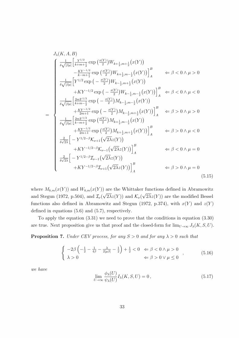
where Mk,m(x(Y )) and Wk,m(x(Y )) are the Whittaker functions defined in Abramowitz
and Stegun (1972, p.504), and Iν(√
2λz(Y )) and Kν(√
2λz(Y )) are the modified Bessel
functions also defined in Abramowitz and Stegun (1972, p.374), with x(Y ) and z(Y )
defined in equations (5.6) and (5.7), respectively.
To apply the equation (3.31) we need to prove that the conditions in equation (3.30)
are true. Next proposition give us that proof and the closed-form for limU→∞ Jλ(K,S, U).
Proposition 7. Under CEV process, for any S > 0 and for any λ > 0 such that−2β
(−1
2− 1
4β− λ
2|µβ| −12
)+ 1
2< 0 ⇐ β < 0 ∧ µ > 0
λ > 0 ⇐ β > 0 ∨ µ ≤ 0, (5.16)
we have
limU→∞
φλ(U)
ψλ(U)Iλ(K,S, U) = 0 , (5.17)
33
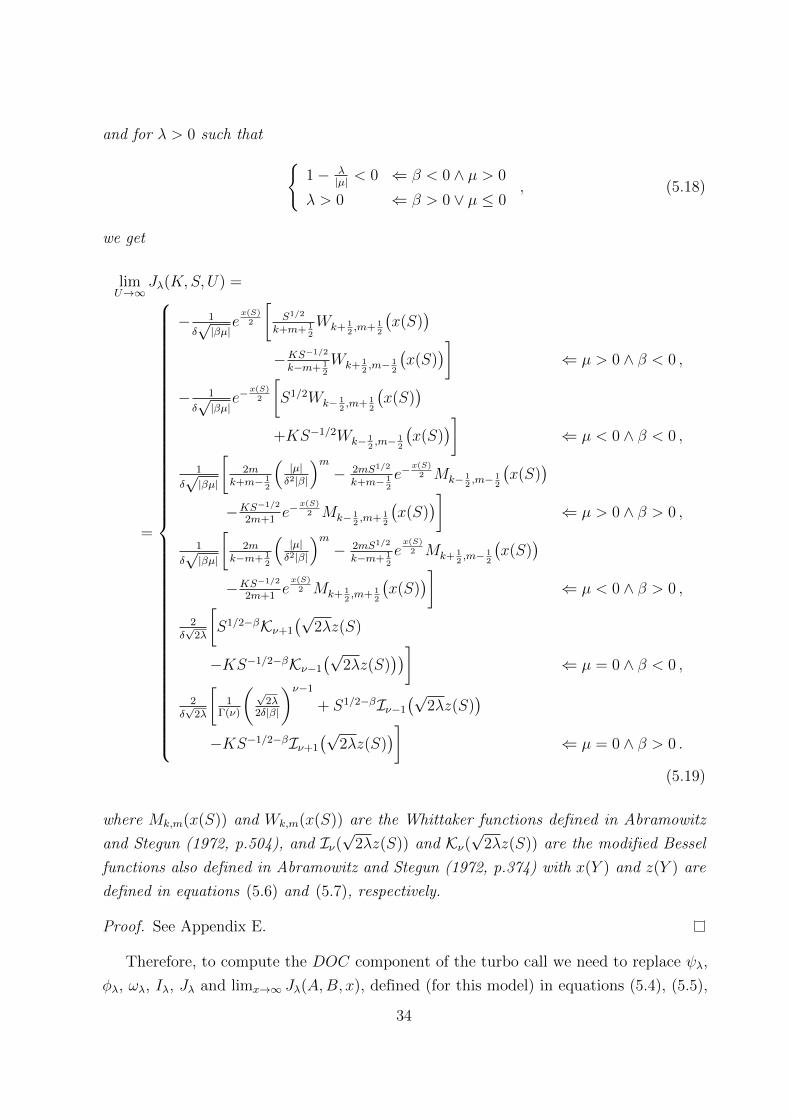
and for λ > 0 such that 1− λ
|µ| < 0 ⇐ β < 0 ∧ µ > 0
λ > 0 ⇐ β > 0 ∨ µ ≤ 0, (5.18)
we get
limU→∞
Jλ(K,S, U) =
=
− 1
δ√|βµ|
ex(S)2
[S1/2
k+m+ 12
Wk+ 12,m+ 1
2
(x(S)
)−KS−1/2
k−m+ 12
Wk+ 12,m− 1
2
(x(S)
)]⇐ µ > 0 ∧ β < 0 ,
− 1
δ√|βµ|
e−x(S)2
[S1/2Wk− 1
2,m+ 1
2
(x(S)
)+KS−1/2Wk− 1
2,m− 1
2
(x(S)
)]⇐ µ < 0 ∧ β < 0 ,
1
δ√|βµ|
[2m
k+m− 12
(|µ|δ2|β|
)m− 2mS1/2
k+m− 12
e−x(S)2 Mk− 1
2,m− 1
2
(x(S)
)−KS−1/2
2m+1e−
x(S)2 Mk− 1
2,m+ 1
2
(x(S)
)]⇐ µ > 0 ∧ β > 0 ,
1
δ√|βµ|
[2m
k−m+ 12
(|µ|δ2|β|
)m− 2mS1/2
k−m+ 12
ex(S)2 Mk+ 1
2,m− 1
2
(x(S)
)−KS−1/2
2m+1ex(S)2 Mk+ 1
2,m+ 1
2
(x(S)
)]⇐ µ < 0 ∧ β > 0 ,
2δ√
2λ
[S1/2−βKν+1
(√2λz(S)
−KS−1/2−βKν−1
(√2λz(S)
))]⇐ µ = 0 ∧ β < 0 ,
2δ√
2λ
[1
Γ(ν)
( √2λ
2δ|β|
)ν−1
+ S1/2−βIν−1
(√2λz(S)
)−KS−1/2−βIν+1
(√2λz(S)
)]⇐ µ = 0 ∧ β > 0 .
(5.19)
where Mk,m(x(S)) and Wk,m(x(S)) are the Whittaker functions defined in Abramowitz
and Stegun (1972, p.504), and Iν(√
2λz(S)) and Kν(√
2λz(S)) are the modified Bessel
functions also defined in Abramowitz and Stegun (1972, p.374) with x(Y ) and z(Y ) are
defined in equations (5.6) and (5.7), respectively.
Proof. See Appendix E.
Therefore, to compute the DOC component of the turbo call we need to replace ψλ,
φλ, ωλ, Iλ, Jλ and limx→∞ Jλ(A,B, x), defined (for this model) in equations (5.4), (5.5),
34
(5.12), (5.14), (5.15) and (5.19), into equation (3.31), using the definition of ∆(A,B) given
in equation (3.23). After that, we have to invert the Laplace transform of (3.31) and
multiply the result by e−r(T−t).
For the LB component we have to invert the Laplace transform of equation (2.10),
replacing φλ defined in equation (5.5) into equation (2.10) to compute F (y;H,T0). The
result must be replace in equation (3.32).
The DR value is obtained by inverting the Laplace transform of equation (3.36),
replacing φλ defined in equation (5.5) into equation (3.36).
Then we have to replace the values of DOC, LB and DR into equation (3.15).
35

Chapter 6
Numerical Analysis
Before presenting the numerical results for turbo warrants, it is necessary to explain
the method used to invert the Laplace transform of equations (2.10), (3.31) and (3.36)
which is required for pricing turbo warrants.
6.1 Euler algorithm
We follow Abate and Whitt (1995, p.37-39) to invert the Laplace transform of equations
(2.10), (3.31) and (3.36). The method described is called the Euler method by the authors
because this method employs Euler summation. Euler summation is one of the more
elementary acceleration techniques. The Euler method is based on the Bromwich contour
inversion integral, which can be expressed as the integral of a real-valued function of a
real variable by choosing a specific contour.
The objective of the Euler method is to calculate values of a real-valued function f(t)
of a positive variable t for various values of t from the Laplace transform
F (s) =
∫ ∞0
e−stf(t)dt ,
where s is a complex variable with a nonnegative real part. Its inversion formula is defined
as follows:
f(t) =1
2πi
∫ a+i∞
a−i∞estF (s)ds ,
where a > 0 is arbitrary, but must be chosen so that it is greater than the real parts of all
the singularities of F (s).
36

Following Abate and Whitt (1995), an approximation of f(t) can be obtained by
f(t) ≈ eA/2
2tRe(F )
(A
2t
)+eA/2
t
∞∑k=1
(−1)kRe(F )
(A+ 2kπi
2t
), (6.1)
where Re(s) is the real part of s and A = 2ta. The approximation above involves a
discretization error. As |f(t)| ≤ 1 for all t, then this error is bonded by
|ed| ≤e−A
1− e−A,
which is approximately equal to e−A when this quantity is small. If we need a discretization
error less than 10−γ, then we let A = γ log(10). In this thesis we use A = 8 log(10) to
achieve a 10−8 discretization error.
To apply the Euler method, we need to truncate the infinite series in equation (6.1) to
n terms. Let sn(t) be this truncation, i.e:
sn(t) =eA/2
2tRe(F )
(A
2t
)+eA/2
t
n∑k=1
(−1)kRe(F )
(A+ 2kπi
2t
). (6.2)
Then we apply the Euler summation to m terms after an initial n, i.e. we compute
the binomial average of the terms sn, sn+1, . . . , sn+m:
E(m,n, t) =m∑k=0
(m
k
)2−msn+k(t) . (6.3)
So, equation (6.3) is an approximation to equation (6.1).
37

6.2 Numerical Results
6.2.1 Lookback Options
Using the pricing formulae derived in sections 4.1 and 5.1 and the Euler algorithm
explained in section 6.1, we obtain the prices of lookback options under the GBM and
CEV models, that are illustrated in Tables 6.1 and 6.2. The first table contains the prices
computed with Matlab(R2010) and the second table contains the prices obtained with
Mathematica(8.0). In all tables, the number of extraterms used in Euler algorithm is
m = 11.
We adopted the same choice of parameters as Davydov and Linetsky (2001): the
initial asset price is S0 = S = 100; the instantaneous volatility at this price level is
σ0 = σ = 25% per annum; the risk-free interest rate is 10% per annum; the asset price
pays no dividend; and all options have six months to expiration (T = 0.5). In the
CEV model, we deploy seven values of β to show its effect on lookback options prices:
β ∈ −4,−3,−2,−1,−0.5, 0.5, 1. Following Davydov and Linetsky (2001), and to ensure
that option prices based on different values of β are comparable, the value of δ is readjusted
so that the initial instantaneous volatility is the same across different models. Then, the
value of δ to be used for the CEV model with different β values is adjusted to δ = σ0S−β0 .
Examination of Tables 6.1 and 6.2 reveals that floating strike lookback call and fixed
strike lookback put options under the CEV model with negative (positive) β are worth
more (less) than under the GBM model. In contrast, floating strike lookback put and fixed
strike lookback call options are worth less (more) under the CEV model with negative
(positive) β than under the GBM model. However, the prices of these contracts when β is
equal to 0.5 are nonsensical. Analysing the two tables we can conclude that the larger the
absolute value of β, the greater the price difference between CEV and GBM option prices.
In the CEV model, the value of β has a greater impact on the prices of lookback options.
Thus, a misspecified value of β may cause very large pricing errors.
Comparing the prices of lookback options under the GBM model, we notice that values
obtained using the Laplace transform are equal to values obtained with Zhang (1998)
formulae. However, if we use Zhang (1998) formulae, the computation time decreases.
If we compare the results of both softwares (Tables 6.1 and 6.2), the prices of lookback
options are almost equals, but we can observe some differences. The prices of fixed strike
lookback call and floating strike lookback put for the CEV model when β = −4 could
not be obtained with Matlab(R2010). The prices of floating strike lookback call and
fixed strike lookback put when β = −0.5 could not be obtained with Matlab(R2010) or
Mathematuca(8.0). Also in the CEV model, when β = −1, the prices obtained with Matlab
38

differ from the prices obtained with Mathematica by more than one tenth. However,
comparing our results with Davydov and Linetsky (2001, Table 2), their prices of lookback
options are closer to our prices obtained with Mathematica (the difference is less than one
hundredth, in this case).
Table 6.1: Prices of lookback options under the CEV and GBM models, computed viaMatlab(R2010)
CEV GBM
βS K -4 -3 -2 -1 -0.5 LT Zhang
Floating strike lookback call
100 N/A 19.5629 18.2922 17.0048 16.3131 NaN 15.6357 15.6357(n = 7) (n = 7) (n = 4) (n = 5) (n = 7) (n = 15)
Fixed strike lookback call
100 100 NaN 14.7988 15.3807 16.1395 16.6083 17.1598 17.1598(n = 7) (n = 7) (n = 7) (n = 7) (n = 7) (n = 15)
100 105 NaN 10.3599 10.9823 11.7748 12.2588 12.8246 12.8246(n = 7) (n = 7) (n = 7) (n = 7) (n = 7) (n = 15)
Floating strike lookback put
100 N/A NaN 9.9217 10.5037 11.2624 11.7312 12.2828 12.2828(n = 7) (n = 7) (n = 7) (n = 7) (n = 7) (n = 15)
Fixed strike lookback put
100 95 10.7897 9.4733 8.1378 7.0764 NaN 6.6631 6.6631(n = 7) (n = 7) (n = 4) (n = 7) (n = 7) (n = 15)
100 100 14.6859 13.4151 12.1277 11.4360 NaN 10.7587 10.7587(n = 7) (n = 7) (n = 4) (n = 5) (n = 7) (n = 15)
CPU time 207,994.05 1.6711 0.0017(in seconds)
The asset price S and the strike price K vary as indicated in first and second columns, respec-tively. The prices of lookback options under the CEV model were calculated with different elasticities,β ∈ −4,−3,−2,−1,−0.5. The number of terms n used in the Euler method is given in parenthesesbelow the corresponding option price. The penultimate and the last columns contain the prices obtained,under the GBM model, using the Laplace Transform (LT) and Zhang (1998) formulae (with the changesmade when r = q), respectively. The last row indicates the computation time for all contracts using theCEV model, the Laplace transform for the GBM model and using Zhang (1998) formulae. The parametersused in the calculations are: σ = 0.25, r = 0.1, q = 0, T = 0.5, m0,T = 100 and M0,T = 100.
39
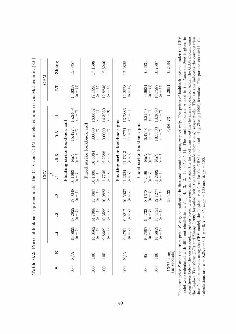
Table
6.2:
Pri
ces
oflo
okbac
kop
tion
sunder
the
CE
Van
dG
BM
mod
els,
com
pute
dvia
Mat
hem
atic
a(8.
0)
CEV
GBM
βS
K-4
-3-2
-1-0.5
0.5
1LT
Zhang
Floatingstrikelookbackcall
100
N/A
19.562
918
.292
217
.004
816
.166
3NaN
15.427
415
.246
815.6357
15.6357
(n=
7)
(n=
7)
(n=
7)
(n=
2)
(n=
7)
(n=
7)
(n=
7)
(n=
15)
Fixed
strikelookbackcall
100
100
14.356
214
.798
815
.380
716
.139
516
.608
40.00
0018
.665
717.1598
17.1598
(n=
7)
(n=
7)
(n=
7)
(n=
7)
(n=
7)
(n=
7)
(n=
1)
(n=
15)
100
105
9.86
6910
.359
910
.982
311
.774
812
.258
80.00
0014
.326
012.8246
12.8246
(n=
7)
(n=
7)
(n=
7)
(n=
7)
(n=
7)
(n=
7)
(n=
3)
(n=
15)
Floatingstrikelookbackput
100
N/A
9.47
919.92
1710
.503
711
.262
411
.731
3-4.877
113
.788
612.2828
12.2828
(n=
7)
(n=
7)
(n=
7)
(n=
7)
(n=
7)
(n=
7)
(n=
1)
(n=
15)
Fixed
strikelookbackput
100
9510
.789
79.47
338.13
787.24
96NaN
6.42
586.21
506.6631
6.6631
(n=
7)
(n=
7)
(n=
7)
(n=
2)
(n=
7)
(n=
7)
(n=
7)
(n=
15)
100
100
14.685
913
.415
112
.127
711
.289
2NaN
10.550
310
.369
810.7587
10.7587
(n=
7)
(n=
7)
(n=
7)
(n=
2)
(n=
7)
(n=
7)
(n=
7)
(n=
15)
CPU
time
595.33
3,48
0.73
1.2951
0.2484
(inseconds)
Theasset
priceSandthestrikepriceK
vary
asindicatedin
firstandsecondcolumns,
respectively.Thepricesoflookback
optionsunder
theCEV
model
werecalculatedwithdifferentelasticities,β∈−
4,−
3,−
2,−
1,−
0.5,0.5,1.
Thenumber
ofterm
snusedin
theEulermethodis
given
inparentheses
below
thecorrespondingoptionprice.Thepen
ultim
ate
andthelast
columnscontain
thepricesobtained
,under
theGBM
model,using
theLaplace
Transform
(LT)andZhang(1998)form
ulae(w
iththech
anges
madewhen
r=q),respectively.Thelast
row
indicatesthecomputation
timeforallcontracts
usingtheCEV
mod
el,theLap
lace
tran
sform
fortheGBM
mod
elan
dusingZhan
g(1998)
form
ulae.
Theparam
etersusedin
the
calculation
sare:σ=
0.25,r=
0.1,q=
0,T
=0.5,m
0,T
=100andM
0,T
=100.
40

Figure 6.1: Price of a floating strike lookback call under the CEV model whenβ = −1, and for different values of n (number of terms used in the Euler method),using Matlab(R2010) and Mathematica(8.0).
0
50
100
150
200
250
300
350
1 2 3 4 5 6 7 8 9 10 11 12 13 14 15
Pric
e of
floa
ting
strik
e lo
okba
ck c
all
n
Mathematica Matlab
(a)
12
16
20
24
28
32
1 2 3 4 5 6
Pric
e of
floa
ting
strik
e lo
okba
ck c
all
n
Matlab
Mathematica
(b)
The parameters used in the calculations are: S = 100, σ = 0.25, r = 0.1, q = 0, T = 0.5, m0,T = 100 andβ = −1. Graph (b) is a zoom of graph (a).
Figure 6.1 illustrates the relationship between the price of a floating strike lookback
call, under the CEV model with β = −1, and the number of terms in the Euler algorithm
(n). Observing Graph 6.2(a), we can notice that if n is a large number, the price of a
floating strike lookback call is nonsensical. In Figure 6.2(b), we observe that a misspecified
41
value of n may cause significant pricing errors, using Matlab(R2010) or Mathematica(8.0).
The same occurs also for fixed strike lookback put options when β = −1. For the case
β = −2, the specification of n is important for floating strike lookback call or fixed strike
lookback put options, when we use Matlab(R2010). The number of terms in the Euler
algorithm (n) used to compute the prices of fixed strike lookback call and floating strike
lookback put options shown in Table 6.2 when β = 1 were chosen so that the values make
sense. So, the methodology proposed by Davydov and Linetsky (2001) is not the best tool
to compute the price of lookback options due to the fact that if we want to know the price
of these contracts, we have to compute them with a large enough value of n for prices to
converge, and we proved that, in some cases, the price of lookback options converges to a
nonsensical value, so we have to choose a small value for n.
42

6.2.2 Turbo Warrants
Using the pricing formulae derived in sections 4.2 and 5.2 and the Euler algorithm
explained in section 6.1, we obtain the prices of turbo call warrants under the GBM
and CEV models, that are illustrated in Tables 6.3 - 6.8. In all tables, the number of
extraterms used in the Euler algorithm is m = 11.
Table 6.3: Prices of turbo call warrants computed under the GBM model and usingMatlab(R2010) when r = q = 5%
σ = 20% σ = 60%
K H T0 LT Zhang LT Zhang
8 9 0.2 1.5739 1.5739 1.1753 1.1753
8 9 0.8 1.4402 1.4402 1.0980 1.0980
7 9 0.2 2.4998 2.4998 1.6735 1.6735
7 9 0.8 2.1823 2.1823 1.3666 1.3666
7 8 0.2 2.7106 2.7106 2.2350 2.2350
7 8 0.8 2.6443 2.6443 2.1596 2.1596
6 8 0.2 3.6541 3.6541 2.8328 2.8328
6 8 0.8 3.5125 3.5125 2.5379 2.5379
CPU time 0.0500 0.0049 0.0540 0.0058(in seconds)
The strike price K and the barrier level H vary as indicated in first and second columns, respectively.The third column contains the time to maturity T0 of the LB component of the turbo call warrant. Thefourth and sixth columns contain the prices obtained under the GBM model, using the Laplace Transform(LT) for σ = 0.2 and σ = 0.6, respectively. The fifth and seventh columns contain the prices obtainedunder the GBM model, using Zhang (1998) formulae (with the changes made when r = q), for σ = 0.2and σ = 0.6, respectively. The last row indicates the computation time for all contracts using the Laplacetransform and Zhang (1998) formulae. The parameters used in the calculations are: S = 10, r = 5%,q = 5% and T = 1. The number of terms n used in the Euler method is 7.
For the GBM model, the parameters adopted are: the initial asset price is S0 = S = 10;
the instantaneous volatility at this price level is σ = 20% per annum or σ = 60%; and all
contracts have one year to expiration (T = 1). In Table 6.3 the risk-free interest rate (r)
and the dividend yield (q) are 5%, in Table 6.4 these parameters are r = 5% and q = 0%,
and in Table 6.5 we have r = 0% and q = 5%.
Examination of the results for the GBM model (Tables 6.3-6.5) reveals that when
increasing the volatility (σ), the price of the turbo call warrant is reduced. We also vary
the strike price (K ∈ 6, 7, 8) and the barrier level (H = 8 or H = 9). When we decrease
the strike price (K) or the barrier level (H), the price of turbo call warrant increases.
43

Table 6.4: Prices of turbo call warrants computed under the GBM model and usingMatlab(R2010) when r = 5% and q = 0%
σ = 20% σ = 60%
K H T0 LT Zhang LT Zhang
8 9 0.2 1.9582 1.9582 1.3366 1.3366
8 9 0.8 1.8508 1.8508 1.2602 1.2602
7 9 0.2 2.8933 2.8933 1.8509 1.8509
7 9 0.8 2.6539 2.6539 1.5511 1.5511
7 8 0.2 3.2019 3.2019 2.5204 2.5204
7 8 0.8 3.1565 3.1565 2.4470 2.4470
6 8 0.2 4.1490 4.1490 3.1365 3.1365
6 8 0.8 4.0578 4.0578 2.8531 2.8531
CPU time 0.0411 0.0050 0.0415 0.0052(in seconds)
The strike price K and the barrier level H vary as indicated in first and second columns, respectively.The third column contains the time to maturity T0 of the LB component of the turbo call warrant. Thefourth and sixth columns contain the prices obtained under the GBM model, using the Laplace Transform(LT) for σ = 0.2 and σ = 0.6, respectively. The fifth and seventh columns contain the prices obtainedunder the GBM model, using Zhang (1998) formulae, for σ = 0.2 and σ = 0.6, respectively. The last rowindicates the computation time for all contracts using the Laplace transform and Zhang (1998) formulae.The parameters used in the calculations are: S = 10, r = 5%, q = 0% and T = 1. The number of terms nused in the Euler method is 7.
These results make sense due to the fact that if the barrier is never touched, the value of
the turbo call warrant is greater. So, if we increase the volatility (or the strike price or
the barrier level), then the probability of the asset price (S) touching the barrier level is
greater. Therefore, the price of the turbo call warrant decreases. For the parameter T0,
we choose two values to compare the results: T0 = 0.2 and T0 = 0.8. This parameter is
the time to maturity of the LB component of the turbo call warrant (that starts when
the barrier level is touched), and is also an important factor because if we increase T0,
the price of a turbo call warrant decreases. This is explained by the increasing of the
probability of the minimum of asset price be less than the strike price (K), because the
time to expiration is bigger.
In the GBM model, the prices of turbo call warrants obtained using the Laplace
transform and Zhang (1998) formulae are equal, but the second method is the fastest.
Comparing the three tables with the GBM model’s results (Tables 6.3 - 6.5), we notice
that increasing the drift (µ = r − q), increases the price of turbo call warrants.
44

Table 6.5: Prices of turbo call warrants computed under the GBM model and usingMatlab(R2010) when r = 0% and q = 5%
σ = 20% σ = 60%
K H T0 LT Zhang LT Zhang
8 9 0.2 1.3057 1.3057 1.0798 1.0798
8 9 0.8 1.1460 1.1460 1.0021 1.0021
7 9 0.2 2.2512 2.2512 1.5728 1.5728
7 9 0.8 1.8513 1.8513 1.2612 1.2612
7 8 0.2 2.3722 2.3722 2.0743 2.0743
7 8 0.8 2.2797 2.2797 1.9969 1.9969
6 8 0.2 3.3542 3.3542 2.6722 2.6722
6 8 0.8 3.1468 3.1468 2.3663 2.3663
CPU time 0.0419 0.0066 0.0503 0.0088(in seconds)
The strike price K and the barrier level H vary as indicated in first and second columns, respectively.The third column contains the time to maturity T0 of the LB component of the turbo call warrant. Thefourth and sixth columns contain the prices obtained under the GBM model, using the Laplace Transform(LT) for σ = 0.2 and σ = 0.6, respectively. The fifth and seventh columns contain the prices obtainedunder the GBM model, using Zhang (1998) formulae, for σ = 0.2 and σ = 0.6, respectively. The last rowindicates the computation time for all contracts using the Laplace transform and Zhang (1998) formulae.The parameters used in the calculations are: S = 10, r = 0%, q = 5% and T = 1. The number of terms nused in the Euler method is 7.
For the CEV model, the parameters adopted are: the initial asset price is S0 = S = 10;
the instantaneous volatility at this price level is σ = 30%; the time to maturity of the LB
component is T0 = 0.8; and all contracts have one year to expiration (T = 1). We also
vary the risk-free interest rate (r) and the dividend-yield (q), studying three cases: r = 5%
and q = 5%, r = 5% and q = 0%, or r = 0% and q = 5%. We deploy seven values of β
to show its effect on lookback options prices: β ∈ −4,−3,−2,−1,−0.5, 0.5, 1. As for
lookback options, the value of δ is readjusted so that the initial instantaneous volatility is
the same across different models. Then, the value of δ to be used for the CEV model with
different β values is adjusted to δ = σS−β0 .
Examination of Tables 6.6 and 6.7 reveals that, in the CEV model with µ ≥ 0
(µ = r − q), when decreasing the strike price (K) or the barrier level (H), the price is
increased. This is explained by the decreasing of the probability of the asset price (S)
touch the barrier (H). There is no a priori rule to the impact on a turbo call price
when β increases or decreases. The value of β has a small impact on the prices of the
turbo warrants; however, a misspecified value of this parameter may cause pricing errors,
45
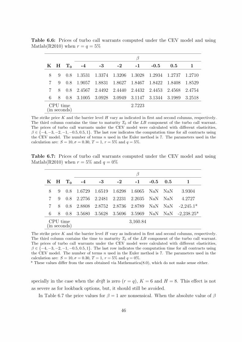
Table 6.6: Prices of turbo call warrants computed under the CEV model and usingMatlab(R2010) when r = q = 5%
β
K H T0 -4 -3 -2 -1 -0.5 0.5 1
8 9 0.8 1.3531 1.3374 1.3206 1.3028 1.2934 1.2737 1.2710
7 9 0.8 1.9057 1.8831 1.8627 1.8467 1.8422 1.8408 1.8529
7 8 0.8 2.4567 2.4492 2.4440 2.4432 2.4453 2.4568 2.4754
6 8 0.8 3.1005 3.0928 3.0949 3.1147 3.1344 3.1989 3.2518
CPU time 2.7223(in seconds)
The strike price K and the barrier level H vary as indicated in first and second columns, respectively.The third column contains the time to maturity T0 of the LB component of the turbo call warrant.The prices of turbo call warrants under the CEV model were calculated with different elasticities,β ∈ −4,−3,−2,−1,−0.5, 0.5, 1. The last row indicates the computation time for all contracts usingthe CEV model. The number of terms n used in the Euler method is 7. The parameters used in thecalculation are: S = 10, σ = 0.30, T = 1, r = 5% and q = 5%.
Table 6.7: Prices of turbo call warrants computed under the CEV model and usingMatlab(R2010) when r = 5% and q = 0%
β
K H T0 -4 -3 -2 -1 -0.5 0.5 1
8 9 0.8 1.6729 1.6519 1.6298 1.6065 NaN NaN 3.9304
7 9 0.8 2.2756 2.2481 2.2231 2.2035 NaN NaN 4.2727
7 8 0.8 2.8808 2.8752 2.8736 2.8789 NaN NaN -2,245.1*
6 8 0.8 3.5680 3.5628 3.5696 3.5969 NaN NaN -2,238.25*
CPU time 3,160.84(in seconds)
The strike price K and the barrier level H vary as indicated in first and second columns, respectively.The third column contains the time to maturity T0 of the LB component of the turbo call warrant.The prices of turbo call warrants under the CEV model were calculated with different elasticities,β ∈ −4,−3,−2,−1,−0.5, 0.5, 1. The last row indicates the computation time for all contracts usingthe CEV model. The number of terms n used in the Euler method is 7. The parameters used in thecalculation are: S = 10, σ = 0.30, T = 1, r = 5% and q = 0%.* These values differ from the ones obtained via Mathematica(8.0), which do not make sense either.
specially in the case when the drift is zero (r = q), K = 6 and H = 8. This effect is not
as severe as for lookback options, but, it should still be avoided.
In Table 6.7 the price values for β = 1 are nonsensical. When the absolute value of β
46

is close to zero, Matlab(R2010) and Mathematica(8.0) programs can not yield any real
values (the results with Mathematica are equal to the results from Maltab, so we decided
publish only the Matlab results). The results in Table 6.8 are completely absurd.
Table 6.8: Prices of turbo call warrants computed under the CEV model and usingMatlab(R2010) when r = 0% and q = 5%
β
K H T0 -4 -3 -2 -1 -0.5 0.5 1
8 9 0.8 -2.7212 -2.3066 -2.0766 -1.8289 NaN NaN 0.6350
7 9 0.8 -2.1959 -1.7883 -1.5624 -1.3135 NaN NaN 0.8951
7 8 0.8 -4.9142 -4.1646 -3.7402 -3.4086 NaN NaN -29.8330*
6 8 0.8 -4.2859 -3.5368 -3.1056 -2.7540 NaN NaN -30.2768*
CPU time 3,143.47(in seconds)
The strike price K and the barrier level H vary as indicated in first and second columns, respectively.The third column contains the time to maturity T0 of the LB component of the turbo call warrant.The prices of turbo call warrants under the CEV model were calculated with different elasticities,β ∈ −4,−3,−2,−1,−0.5, 0.5, 1. The last row indicates the computation time for all contracts usingthe CEV model. The number of terms n used in the Euler method is 7. The parameters used in thecalculation are: S = 10, σ = 0.30, T = 1, r = 0% and q = 5%.* These values differ from the ones obtained via Mathematica(8.0).
47
Chapter 7
Conclusion
This thesis studies the pricing of turbo warrants and lookback options under the GBM
and CEV models. Following Davydov and Linetsky (2001), we derived pricing solutions
for lookback options in closed-form, and following Wong and Chan (2008), we derived
pricing solutions for turbo call warrants also in closed-form.
For the GBM model, we compared two different methods to compute the prices of
lookback options: the Laplace transform of the probability distributions of the minimum
and maximum asset prices, and the Zhang (1998) formulae.1 We conclude that both
methods produce the same prices, but Laplace transform is the slowest method. We did
the same comparison for turbo call warrants: we compared Laplace transforms of the
probability distributions of the minimum and maximum asset prices and of the expected
value of the terminal payoff of a double knock out option against Zhang (1998) formulae.
The conclusion is the same: the Laplace transform methodology is the slowest one.
For the CEV model, the variation of β influences the price of lookback options: when
β is increased, the price of floating strike lookback call (put) and fixed strike lookback
put (call) options increases (decreases). For turbo warrants, the results did not provide
any pattern. Therefore, lookback options and turbo call warrants are sensitive to the
specification of the elasticity parameter β, and because of that errors can exist in the price
of these contracts if the estimation of β is incorrect.
Although we have obtained closed-form solutions to price these contracts under the
CEV model, the results are not good enough: in same cases, we had to choose a number
of terms (n) to invert the Laplace transform numerically different from the pre-specified
one, because the option price converges to a nonsensical number; in other cases, we did
not obtain prices for an absolute value of β near zero; for β > 0, not all the values made
sense; and when the risk-free rate is smaller than the dividend yield (r < q), the prices of
1However, for r = q this formulae is incorrect, so we had to derive the prices of these contracts.
48

turbo warrants were nonsensical.
49

Appendix A
Proof of Proposition 1
Before deriving equations (2.18) to (2.21), we need to follow some steps:
1. We need to show that
(X −m0,T )+ =
∫ X
0
11m0,T≤ydy ∀X ∈ R+ . (A.1)
Let y ∈ [0, X] and
11m0,T≤y =
1 ⇐ y ≥ m0,T
0 ⇐ y < m0,T
.
If X ≥ m0,T , then ∫ X
0
11m0,T≤ydy =
∫ X
m0,T
1dy
= X −m0,T .
If X < m0,T , then y ≤ X < m0,T and 11m0,T≤y = 0 . Thus,
∫ X
0
11m0,T≤ydy = 0 .
Hence, ∫ X
0
11m0,T≤ydy =
X −m0,T ⇐ X ≥ m0,T
0 ⇐ X < m0,T
= (X −m0,T )+ .
50
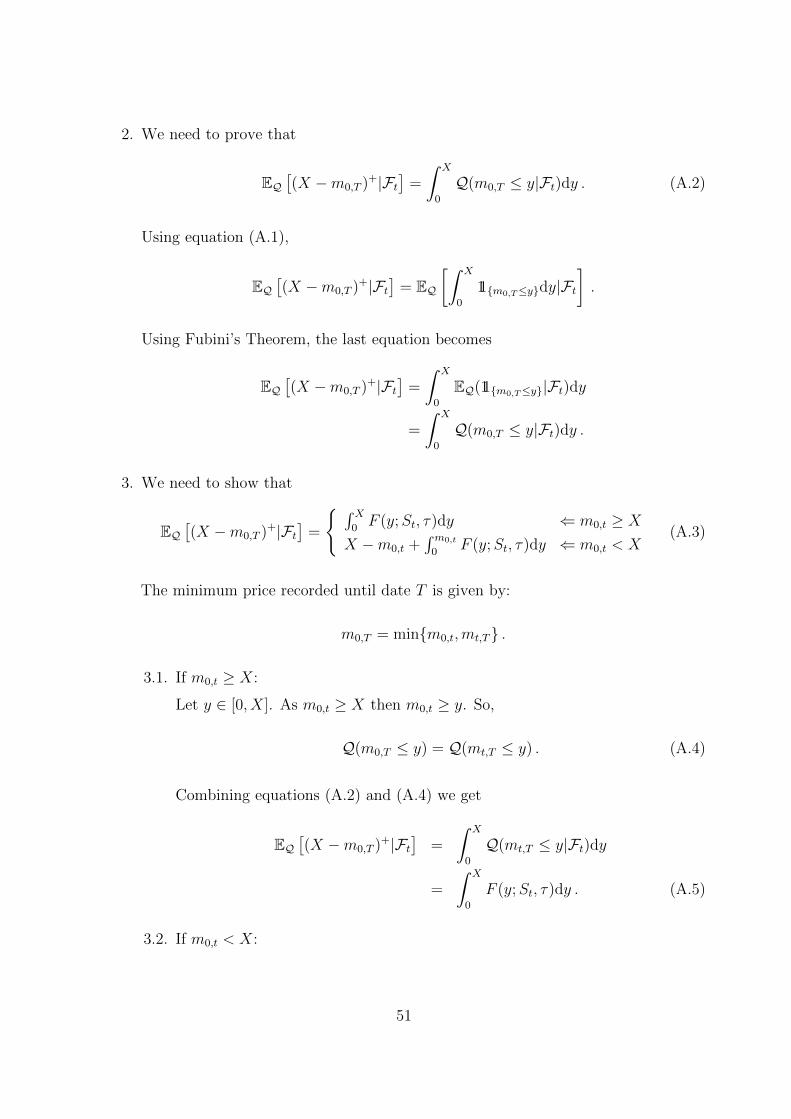
2. We need to prove that
EQ[(X −m0,T )+|Ft
]=
∫ X
0
Q(m0,T ≤ y|Ft)dy . (A.2)
Using equation (A.1),
EQ[(X −m0,T )+|Ft
]= EQ
[∫ X
0
11m0,T≤ydy|Ft].
Using Fubini’s Theorem, the last equation becomes
EQ[(X −m0,T )+|Ft
]=
∫ X
0
EQ(11m0,T≤y|Ft)dy
=
∫ X
0
Q(m0,T ≤ y|Ft)dy .
3. We need to show that
EQ[(X −m0,T )+|Ft
]=
∫ X0F (y;St, τ)dy ⇐ m0,t ≥ X
X −m0,t +∫ m0,t
0F (y;St, τ)dy ⇐ m0,t < X
(A.3)
The minimum price recorded until date T is given by:
m0,T = minm0,t,mt,T .
3.1. If m0,t ≥ X:
Let y ∈ [0, X]. As m0,t ≥ X then m0,t ≥ y. So,
Q(m0,T ≤ y) = Q(mt,T ≤ y) . (A.4)
Combining equations (A.2) and (A.4) we get
EQ[(X −m0,T )+|Ft
]=
∫ X
0
Q(mt,T ≤ y|Ft)dy
=
∫ X
0
F (y;St, τ)dy . (A.5)
3.2. If m0,t < X:
51

Using equation (A.2), then
EQ[(X −m0,T )+|Ft
]=
∫ X
0
Q(m0,T ≤ y|Ft)dy
=
∫ m0,t
0
Q(m0,T ≤ y|Ft)dy +
∫ X
m0,t
Q(m0,T ≤ y|Ft)dy
=
∫ m0,t
0
Q(m0,T ≤ y|Ft)dy +
∫ X
m0,t
1 dy .
The last equality arises because m0,T ≤ m0,t.
Let y ∈ [0,m0,t]. As m0,T = minm0,t,mt,T, then m0,T ≤ y ⇔ mt,T ≤ y.
Therefore,
EQ[(X −m0,T )+|Ft
]=
∫ m0,t
0
Q(mt,T ≤ y|Ft)dy +X −m0,t
=
∫ m0,t
0
F (y;St, τ)dy +X −m0,t . (A.6)
Combining the equations (A.5) and (A.6), equation (A.3) arises.
4. Proof of equations (2.18) and (2.21).
The terminal payoff of a floating strike lookback call on asset S and with expiry
date at time T is LCfl(T ;ST ,m0,T , T ) = ST −m0,T . The value at any time t < T of
the floating strike lookback call is:
LCfl(t;St,m0,t, T ) = e−rτEQ [ST −m0,T |Ft]
= e−rτ(EQ [ST −m0,t|Ft] + EQ [m0,t −m0,T |Ft]
)= e−rτEQ(ST |Ft)− e−rτm0,t + e−rτEQ(m0,t −m0,T |Ft)
= e−rτSte(r−q)τ − e−rτm0,t + e−rτEQ
[(m0,t −m0,T )+|Ft
].
(A.7)
The last equation was obtained due to the fact that EQ(ST |Ft) = Ste(r−q)τ and
m0,T ≤ m0,t.
Combining equations (A.7) and (A.3) and replacing X for m0,t,
LCfl(t;St,m0,t, T ) = e−qτSt − e−rτm0,t + e−rτ∫ m0,t
0
F (y;St, τ)dy ,
and equation (2.18) follows.
52
The terminal payoff of a fixed strike lookback put on asset S, with strike price K
and expiry date at time T is LPfx(T ;ST , K,m0,T , T ) = (K −m0,T )+.
The value at any time t < T of the fixed strike lookback put is obtained by replacing
X for K in equation (A.3) and discounting, which yields equation (2.21).
5. We need to show that
(M0,T −X)+ =
∫ ∞X
11M0,T≥ydy ∀X ∈ R+ . (A.8)
Let y ∈ [X,∞[ and
11M0,T≥y =
1 ⇐ y ≤M0,T
0 ⇐ y > M0,T
If X ≤M0,T , then ∫ ∞X
11M0,T≥ydy =
∫ M0,T
X
1dy
= M0,T −X .
If X > M0,T , then y ≥ X > M0,T and 11M0,T≥y = 0 . Thus,∫ ∞X
11M0,T≥ydy = 0 .
Hence, ∫ ∞X
11M0,T≥ydy =
M0,T −X ⇐ X ≤M0,T
0 ⇐ X > M0,T
= (M0,T −X)+ .
6. We need to prove that
EQ[(M0,T −X)+|Ft
]=
∫ ∞X
Q(M0,T ≥ y|Ft)dy . (A.9)
Using equation (A.8),
EQ[(M0,T −X)+|Ft
]= EQ
[∫ ∞X
11M0,T≥ydy|Ft].
53
Using Fubini’s Theorem, the last equation becomes
EQ[(M0,T −X)+|Ft
]=
∫ ∞X
EQ(11M0,T≥y|Ft)dy
=
∫ ∞X
Q(M0,T ≥ y|Ft)dy .
7. We need to show that
EQ[(M0,T −X)+|Ft
]=
∫∞XG(y;St, τ)dy ⇐M0,t ≤ X
M0,t −X +∫∞M0,t
G(y;St, τ)dy ⇐M0,t > X(A.10)
The maximum price recorded until date T is given by:
M0,T = maxM0,t,Mt,T
7.1. If M0,t ≤ X:
Let y ∈ [X,∞[. As M0,t ≤ X then M0,t ≤ y. So,
Q(M0,T ≥ y) = Q(Mt,T ≥ y) . (A.11)
Combining equations (A.9) and (A.11) we get
EQ[(M0,T −X)+|Ft
]=
∫ ∞X
Q(Mt,T ≥ y|Ft)dy
=
∫ ∞X
G(y;St, τ)dy . (A.12)
7.2. If M0,t > X:
Using equation (A.9), then
EQ[(M0,T −X)+|Ft
]=
∫ ∞X
Q(M0,T ≥ y|Ft)dy
=
∫ M0,t
X
Q(M0,T ≥ y|Ft)dy +
∫ ∞M0,t
Q(M0,T ≥ y|Ft)dy
=
∫ M0,t
X
1 dy +
∫ ∞M0,t
Q(M0,T ≥ y|Ft)dy .
The last equality arises because M0,T ≥M0,t.
54
Let y ∈ [M0,t,∞[. As M0,T = maxM0,t,Mt,T, then M0,T ≥ y ⇔ Mt,T ≥ y.
Therefore,
EQ[(M0,T −X)+|Ft
]= M0,t −X +
∫ ∞M0,t
Q(Mt,T ≥ y|Ft)dy
= M0,t −X +
∫ ∞M0,t
G(y;St, τ)dy . (A.13)
Combining the equations (A.12) and (A.13), equation (A.10) arises.
8. Proof of equations (2.19) and (2.20).
The terminal payoff of a floating strike lookback put on asset S and with expiry
date at time T is LPfl(T ;ST ,M0,T , T ) = M0,T − ST . The value at any time t < T
of the floating strike lookback call is:
LPfl(t;St,M0,t, T ) = e−rτEQ [M0,T − ST |Ft]
= e−rτ(EQ [M0,T −M0,t|Ft]
)+ e−rτ
(EQ [M0,t − ST |Ft]
)= e−rτEQ(M0,T −M0,t|Ft) + e−rτM0,t − e−rτEQ(ST |Ft)
= e−rτEQ[(M0,T −M0,t)
+|Ft]
+ e−rτM0,t − e−rτSte(r−q)τ .
(A.14)
This last equation was obtained due to the fact that EQ(ST |Ft) = Ste(r−q)τ and
M0,T ≥M0,t.
Combining equations (A.14) and (A.10) and replacing X for M0,t,
LPfl(t;St,M0,t, T ) = e−rτ∫ ∞M0,t
G(y;St, τ)dy + e−rτM0,t − e−qτSt ,
and equation (2.19) follows.
The terminal payoff of a fixed strike lookback call on asset S, with strike price K
and expiry date at time T is LCfx(T ;ST , K,M0,T , T ) = (M0,T −K)+.
The value at any time t < T of the fixed strike lookback call is obtained replacing
X for K in equation (A.10) and discounting, which yields equation (2.20).
55

Appendix B
Proof of Proposition 3
Following Davydov and Linetsky (2001),
τ(L,U) := inft ≥ 0 : St /∈ (L,U) ,
and, therefore,
∫ ∞0
e−λTEQ[11τ(L,U)>T(ST −K)+]dT =
∫ ∞0
e−λT
[∫ U
L
(Y −K)+p(T ;S;Y )dY
]dT ,
where p(t;S;Y ) is the transition density of the diffusion St : t ≥ 0, starting at S0 = S,
with respect to the speed measure (see Borodin and Salminen, 1996, p.13). We are
studying the case where the strike price (K) is less than the downside barrier (L), so we
get (Y −K)+ = Y −K because the Y is between the downside barrier (L) and upper
barrier (U). Using Fubbini’s Theorem:
∫ ∞0
e−λTEQ[11τ(L,U)>T(ST −K)+]dT =
∫ U
L
(Y −K)
[∫ ∞0
e−λTp(T ;S;Y )dT
]dY .
The second integral on the right-hand side of the previous equation is the Green’s
function, Gλ(S, Y ), defined in Borodin and Salminen (1996, p.19). Therefore,∫ ∞0
e−λTEQ[11τ(L,U)>T(ST −K)+]dT =
∫ U
L
(Y −K)Gλ(S, Y )dY . (B.1)
The Green’s function can be written as (see Ferreira (2009, p. 14-15) or Davydov and
56

Linetsky (2001, p. 962) for details):
Gλ(S, Y )dY =
m(Y )
ωλ∆λ(L,U)∆λ(L, S)∆λ(Y, U) if S ≤ Y
m(Y )ωλ∆λ(L,U)
∆λ(L, Y )∆λ(S, U) if S > Y. (B.2)
As S ∈ [L,U ] (by definition of the double barrier option), then∫ U
L
(Y −K)Gλ(S, Y )dY =
∫ S
L
(Y −K)Gλ(S, Y )dY +
∫ U
S
(Y −K)Gλ(S, Y )dY . (B.3)
When Y ∈ [L, S] then S > Y , and if Y ∈ [S, U ] then S ≤ Y. Applying equation (B.2) to
the first and second integrals on the right-hand side of equation (B.3), we get∫ U
L
(Y −K)Gλ(S, Y )dY =
∫ S
L
(Y −K)m(Y )
ωλ∆λ(L,U)∆λ(L, Y )∆λ(S, U)dY
+
∫ U
S
(Y −K)m(Y )
ωλ∆λ(L,U)∆λ(L, S)∆λ(Y, U)dY
=∆λ(S, U)
ωλ∆λ(L,U)
∫ S
L
(Y −K)m(Y )∆λ(L, Y )dY
+∆λ(L, S)
ωλ∆λ(L,U)
∫ U
S
(Y −K)m(Y )∆λ(Y, U)dY . (B.4)
Using equation (3.23), equation (B.4) can be written as∫ U
L
(Y −K)Gλ(S, Y )dY
=1
ωλ∆λ(L,U)
[∆λ(S, U)
∫ S
L
(Y −K)m(Y )(φλ(L)ψλ(Y )− ψλ(L)φλ(Y )
)dY
+∆λ(L, S)
∫ U
S
(Y −K)m(Y )(φλ(Y )ψλ(U)− ψλ(Y )φλ(U)
)dY]
=1
ωλ∆λ(L,U)
∆λ(S, U)
[φλ(L)
∫ S
L
(Y −K)m(Y )ψλ(Y )dY
−ψλ(L)
∫ S
L
(Y −K)m(Y )φλ(Y )dY]
+∆λ(L, S)[ψλ(U)
∫ U
S
(Y −K)m(Y )φλ(Y )dY
−φλ(U)
∫ U
S
(Y −K)m(Y )ψλ(Y ))dY]. (B.5)
57

Using definitions (3.24) and (3.25) as well as equations (B.1) and (B.5), it follows that∫ ∞0
e−λTEQ[11τ(L,U)>T(ST −K)+]dT
=1
ωλ∆λ(L,U)
[∆λ(S, U)
[φλ(L)Iλ(K,L, S)− ψλ(L)Jλ(K,L, S)
]+∆λ(L, S)
[ψλ(U)Jλ(K,S, U)− φλ(U)Iλ(K,S, U)
]],
which is exactly the equation (3.31).
58

Appendix C
Proof of equations (4.6) - (4.9)
To prove equations (4.6) - (4.9) for the case that r = q we determine the limit of these
equations when r 6= q as r − q approaches zero.
First, we need to show that
limr−q→0
(− dbs1(X, Y )
)= lim
r−q→0
(dbs(Y,X)
)(C.1)
Using equations (4.10) and (4.11), we get
limr−q→0
(− dbs1(X, Y )
)= lim
r−q→0
(− ln(X/Y ) + (r − q + σ2/2)τ
σ√τ
)=
ln(Y/X)− σ2
2τ
σ√τ
= limr−q→0
(ln(Y/X) + (r − q − σ2/2)τ
σ√τ
)= lim
r−q→0
(dbs(Y,X)
).
Then we can proceed to the calculation of the limit for the lookback options as r − qapproaches zero.
1. Proof of equation (4.6).
59
limr−q→0
LCfl(t;St,m0,t, T )
= limr−q→0
(Ste−qτΦ[dbs1(St,m0,t)]−m0,te
−rτΦ[dbs(St,m0,t)]
+Stδ
e−rτ
(Stm0,t
)−δΦ[dbs(m0,t, St)]− e−qτΦ[−dbs1(St,m0,t)]
)= Ste
−qτΦ[dbs1(St,m0,t)]−m0,te−rτΦ[dbs(St,m0,t)]
+Ste−rτ σ
2
2lim
r−q→0
(
Stm0,t
)− 2(r−q)σ2
Φ[dbs(m0,t, St)]− e(r−q)τΦ[−dbs1(St,m0,t)]
r − q
.
(C.2)
The last equation arises because δ = 2(r−q)σ2 . When we replace the expression r − q
by zero in the last equation we obtain an indeterminate 0/0 form. Applying the
L’Hospital’s rule, the indeterminate found becomes
limr−q→0
(
Stm0,t
)− 2(r−q)σ2
Φ[dbs(m0,t, St)]− e(r−q)τΦ[−dbs1(St,m0,t)]
r − q
= lim
r−q→0
− 2
σ2ln
(Stm0,t
)(Stm0,t
)− 2(r−q)σ2
Φ[dbs(m0,t, St)]
+
(Stm0,t
)− 2(r−q)σ2
f [dbs(m0,t, St)]
√τ
σ− τe(r−q)τΦ[−dbs1(St,m0,t)]
−e(r−q)τf [−dbs1(St,m0,t)]
(−√τ
σ
), (C.3)
where the last equation arises when we evaluate the derivatives of numerator and
denominator with respect to r − q. Note that the derivative of dbs(Y,X) and
dbs1(Y,X) are given by
∂dbs(Y,X)
∂(r − q)=
∂
∂(r − q)
(ln(Y/X) + (r − q − σ2/2)τ
σ√τ
)=
τ
σ√τ
=
√τ
σ, (C.4)
60
and
∂dbs1(Y,X)
∂(r − q)=
∂
∂(r − q)
(ln(Y/X) + (r − q + σ2/2)τ
σ√τ
)=
τ
σ√τ
=
√τ
σ. (C.5)
Using equation (C.1), and determining the limit of equation (C.3), we get
limr−q→0
(
Stm0,t
)− 2(r−q)σ2
Φ[dbs(m0,t, St)]− e(r−q)τΦ[−dbs1(St,m0,t)]
r − q
= − 2
σ2ln
(Stm0,t
)Φ[−dbs1(St,m0,t)] +
√τ
σf [−dbs1(St,m0,t)]
−τΦ[−dbs1(St,m0,t)] +
√τ
σf [−dbs1(St,m0,t)]
=2√τ
σf [−dbs1(St,m0,t)]− Φ[−dbs1(St,m0,t)]
2
σ2ln
(Stm0,t
)+ τ
.
Combining the last equation with equation (C.2), we get
limr−q→0
LCfl(t;St,m0,t, T )
= Ste−qτΦ[dbs1(St,m0,t)]−m0,te
−rτΦ[dbs(St,m0,t)]
+Ste−rτ σ
2
2
(2√τ
σf [−dbs1(St,m0,t)]− Φ[−dbs1(St,m0,t)]
2
σ2ln
(Stm0,t
)+ τ
)= Ste
−qτΦ[dbs1(St,m0,t)]−m0,te−rτΦ[dbs(St,m0,t)]
+Ste−rτσ√τf [−dbs1(St,m0,t)]
−Ste−rτσ2
2Φ[−dbs1(St,m0,t)]
2
σ2ln
(Stm0,t
)+ τ
,
which is the equation (4.6) when r = q.
61

2. Proof of equation (4.7).
limr−q→0
LPfl(t;St, K,M0,t, T )
= limr−q→0
(M0,te
−rτΦ[−dbs(St,M0,t)]− Ste−qτΦ[−dbs1(St,M0,t)]
+Stδ
e−qτΦ[dbs1(St,M0,t)]− e−rτ
(StM0,t
)−δΦ[−dbs(M0,t, St)]
)= M0,te
−rτΦ[−dbs(St,M0,t)]− Ste−qτΦ[−dbs1(St,M0,t)]
+Ste−rτ σ
2
2lim
r−q→0
e(r−q)τΦ[dbs1(St,M0,t)]−(
StM0,t
)− 2(r−q)σ2
Φ[−dbs(M0,t, St)]
r − q
,
(C.6)
using the definition of δ provided in equation (4.12). When we replace the expression
r − q by zero in the last equation we obtain an indeterminate 0/0 form. Applying
the L’Hospital’s rule, the indeterminate found becomes
limr−q→0
e(r−q)τΦ[dbs1(St,M0,t)]−(
StM0,t
)− 2(r−q)σ2
Φ[−dbs(M0,t, St)]
r − q
= lim
r−q→0
τe(r−q)τΦ[dbs1(St,M0,t)] + e(r−q)τf [dbs1(St,M0,t)]
(√τ
σ
)
−(− 2
σ2
)ln
(StM0,t
)(StM0,t
)− 2(r−q)σ2
Φ[−dbs(M0,t, St)]
−(
StM0,t
)− 2(r−q)σ2
f [−dbs(M0,t, St)]
(−√τ
σ
), (C.7)
where the last equation arises when we evaluate the derivatives of numerator and
denominator with respect to r − q. Note that the derivative of dbs(Y,X) and
dbs1(Y,X) are given by equations (C.4) and (C.5).
62

Using equation (C.1), the equation (C.7) becomes,
limr−q→0
e(r−q)τΦ[dbs1(St,M0,t)]−(
StM0,t
)− 2(r−q)σ2
Φ[−dbs(M0,t, St)]
r − q
= τΦ[dbs1(St,M0,t)] +
√τ
σf [dbs1(St,M0,t)]
+2
σ2ln
(StM0,t
)Φ[dbs1(St,M0,t)] +
√τ
σf [dbs1(St,M0,t)]
=2√τ
σf [dbs1(St,M0,t)] + Φ[dbs1(St,M0,t)]
2
σ2ln
(StM0,t
)+ τ
.
Combining the last equation with equation (C.6), we get
limr−q→0
LPfl(t;St, K,M0,t, T )
= M0,te−rτΦ[−dbs(St,M0,t)]− Ste−qτΦ[−dbs1(St,M0,t)]
+Ste−rτ σ
2
2
(2√τ
σf [dbs1(St,M0,t)] + Φ[dbs1(St,M0,t)]
2
σ2ln
(StM0,t
)+ τ
)= M0,te
−rτΦ[−dbs(St,M0,t)]− Ste−qτΦ[−dbs1(St,M0,t)]
+Ste−rτσ√τf [dbs1(St,M0,t)]
+Ste−rτ σ
2
2Φ[dbs1(St,M0,t)]
2
σ2ln
(StM0,t
)+ τ
, (C.8)
which is equation (4.7) for the case r = q.
3. Proof of equation (4.8).
Using the same arguments applied to the proofs of equations (4.6) and (4.7), we
obtain a similar result for the equation (4.8).
limr−q→0
LCfx(t;St, K,M0,t, T )
= limr−q→0
(e−rτ
(M0,t −K
)++ Ste
−qτΦ[dbs1(St,maxM0,t, K)]
−maxM0,t, Ke−rτΦ[dbs(St,maxM0,t, K)]
+Stδ
e−qτΦ[dbs1(St,maxM0,t, K)]
−e−rτ(
StmaxM0,t, K
)−δΦ[−dbs(maxM0,t, K, St)]
)
63

To simplify the expression, let M = maxM0,t, K. Then
limr−q→0
LCfx(t;St, K,M0,t, T )
= e−rτ(M0,t −K
)++ Ste
−qτΦ[dbs1(St,M)]−Me−rτΦ[dbs(St,M)]
+Ste−rτ σ
2
2lim
r−q→0
(e(r−q)τΦ[dbs1(St,M)]−
(StM
)− 2(r−q)σ2
Φ[−dbs(M,St)]
r − q
)= e−rτ
(M0,t −K
)++ Ste
−qτΦ[dbs1(St,M)]−Me−rτΦ[dbs(St,M)]
+Ste−rτ σ
2
2lim
r−q→0
(τe(r−q)τΦ[dbs1(St,M)] + e(r−q)τf [dbs1(St,M)]
(√τ
σ
)
−(− 2
σ2
)ln
(StM
)(StM
)− 2(r−q)σ2
Φ[−dbs(M,St)]
−(StM
)− 2(r−q)σ2
f [−dbs(M,St)]
(−√τ
σ
))= e−rτ
(M0,t −K
)++ Ste
−qτΦ[dbs1(St,M)]−Me−rτΦ[dbs(St,M)]
+Ste−rτ σ
2
2
(τΦ[dbs1(St,M)] +
√τ
σf [dbs1(St,M)] +
2
σ2ln
(StM
)Φ[dbs1(St,M)]
+
√τ
σf [dbs1(St,M)]
)= e−rτ
(M0,t −K
)++ Ste
−qτΦ[dbs1(St,M)]−Me−rτΦ[dbs(St,M)]
+Ste−rτσ
√(τ)f [dbs1(St,M)] + Ste
−rτ σ2
2Φ[dbs1(St,M)]
2
σ2ln
(StM
)+ τ
,
which is the equation (4.8), when r = q.
4. Proof of equation (4.9). Using the same arguments applied to the proofs of equations
(4.6) - (4.8), we obtain a similar result for the equation (4.9).
limr−q→0
LPfx(t;St, K,M0,t, T )
= limr−q→0
(e−rτ
(K −m0,t
)++ minm0,t, Ke−rτΦ[−dbs(St,minm0,t, K)]
−Ste−qτΦ[−dbs1(St,minm0,t, K)] +Stδ
− e−qτΦ[−dbs1(St,minm0,t, K)]
+e−rτ(
Stminm0,t, K
)−δΦ[dbs(minm0,t, K, St)]
)
64
To simplify the expression, let m = minm0,t, K. Therefore,
limr−q→0
LPfx(t;St, K,M0,t, T )
= e−rτ(K −m0,t
)++me−rτΦ[−dbs(St,m)]− Ste−qτΦ[−dbs1(St,m)]
+Ste−rτ σ
2
2lim
r−q→0
(−e(r−q)τΦ[−dbs1(St,m)] +(Stm
)− 2(r−q)σ2
Φ[dbs(m,St)]
r − q
)= e−rτ
(K −m0,t
)++me−rτΦ[−dbs(St,m)]− Ste−qτΦ[−dbs1(St,m)]
+Ste−rτ σ
2
2lim
r−q→0
− τe(r−q)τΦ[−dbs1(St,m)]
−e(r−q)τf [−dbs1(St,m)]
(−√τ
σ
)+
(− 2
σ2
)ln
(Stm
)(Stm
)− 2(r−q)σ2
Φ[dbs(m,St)]
+
(Stm
)− 2(r−q)σ2
f [dbs(m,St)]
(√τ
σ
)= e−rτ
(K −m0,t
)++me−rτΦ[−dbs(St,m)]− Ste−qτΦ[−dbs1(St,m)]
+Ste−rτ σ
2
2
− τΦ[−dbs1(St,m)] +
√τ
σf [−dbs1(St,m)]
− 2
σ2ln
(Stm
)Φ[−dbs1(St,m)] +
√τ
σf [−dbs1(St,m)]
= e−rτ
(K −m0,t
)++me−rτΦ[−dbs(St,m)]− Ste−qτΦ[−dbs1(St,m)]
+Ste−rτσ√τf [−dbs1(St,m)]− Ste−rτ
σ2
2Φ[−dbs(St,m)]
2
σ2ln
(Stm
)+ τ
,
which is the equation (4.9) for the case r = q.
65

Appendix D
Proof of Proposition 5
To prove Proposition 5 we will use equations (4.2), (4.3), (4.4), (4.5), (4.17) and (4.18):
limU→∞
φλ(U)
ψλ(U)Iλ(K,S, U) = lim
U→∞
Uγ−
Uγ+
2
σ2
(U1−γ−
1− γ−+K
U−γ−
γ−− S1−γ−
1− γ−−KS−γ−
γ−
)=
2
σ2limU→∞
U1−γ+(
1
1− γ−+K
U−1
γ−
)− 2
σ2
(S1−γ−
1− γ−+K
S−γ−
γ−
)limU→∞
Uγ−−γ+ . (D.1)
Using the definitions of γ− and γ+ provided in equation (4.4), we get
1− γ+ = 1 + γ −√γ2 +
2λ
σ2, (D.2)
i.e.
1− γ+ < 0 , (D.3)
as long as λ is large enough for inequality (4.19) to be verified.
And
γ− − γ+ = −γ −√γ2 +
2λ
σ2+ γ −
√γ2 +
2λ
σ2
= −2
√γ2 +
2λ
σ2, (D.4)
i.e.
γ− − γ+ < 0 . (D.5)
66
Using equations (D.3) and (D.5), the equation (D.1) becomes
limU→∞
φλ(U)
ψλ(U)Iλ(K,S, U) = 0 . (D.6)
For the integral Jλ(K,S, U), equation (5.15) yields:
limU→∞
Jλ(K,S, U) = limU→∞
2
σ2
(U1−γ+
1− γ+
+KU−γ+
γ+
− S1−γ+
1− γ+
−KS−γ+
γ+
)=
2
σ2limU→∞
(U1−γ+
1− γ+
+KU−γ+
γ+
)− 2
σ2
(S1−γ+
1− γ+
+KS−γ+
γ+
). (D.7)
Using the definition of γ+ provided in equation (4.4), it follows that
− γ+ = γ −√γ2 +
λ
σ2. (D.8)
As γ ≤√γ2 and
√γ2 <
√γ2 + 2λ
σ2 (because λ > 0), the expression −γ+ in equation
(D.8) is negative.
Using equations (D.8) and (D.3), equation (D.7) becomes
limU→∞
Jλ(K,S, U) = − 2
σ2
(S1−γ+
1− γ+
+KS−γ+
γ+
). (D.9)
67
Appendix E
Proof of Proposition 7
To prove Proposition 7 we will use equations (5.4)-(5.11), (5.14) and (5.15).
• If µ > 0 and β < 0
limU→∞
φλ(U)
ψλ(U)Iλ(K,S, U)
= limU→∞
Uβ+ 12 e
ε2x(U)Wk,m(x(U))
Uβ+ 12 e
ε2x(U)Mk,m(x(U))
1
δ√|βµ|
[U1/2
2m+ 1exp
(x(U)
2
)Mk+ 1
2,m+ 1
2
(x(U)
)−2mKU−1/2
m− k − 12
exp
(x(U)
2
)Mk+ 1
2,m− 1
2
(x(U)
)− S1/2
2m+ 1exp
(x(S)
2
)Mk+ 1
2,m+ 1
2
(x(S)
)+
2mKS−1/2
m− k − 12
exp
(x(S)
2
)Mk+ 1
2,m− 1
2
(x(S)
)]
=1
δ√|βµ|
limU→∞
Wk,m(x(U))
Mk,m(x(U))exp
(x(U)
2
)U1/2
[1
2m+ 1Mk+ 1
2,m+ 1
2
(x(U)
)− 2mKU−1
m− k − 12
Mk+ 12,m− 1
2
(x(U)
)]
− 1
δ√|βµ|
[S1/2
2m+ 1exp
(x(S)
2
)Mk+ 1
2,m+ 1
2
(x(S)
)−2mKS−1/2
m− k − 12
exp
(x(S)
2
)Mk+ 1
2,m− 1
2
(x(S)
)]limU→∞
(Wk,m(x(U))
Mk,m(x(U))
).
Using equations (13.1.32) and (13.1.33) of Abramowitz and Stegun (1972, p.505) the
68
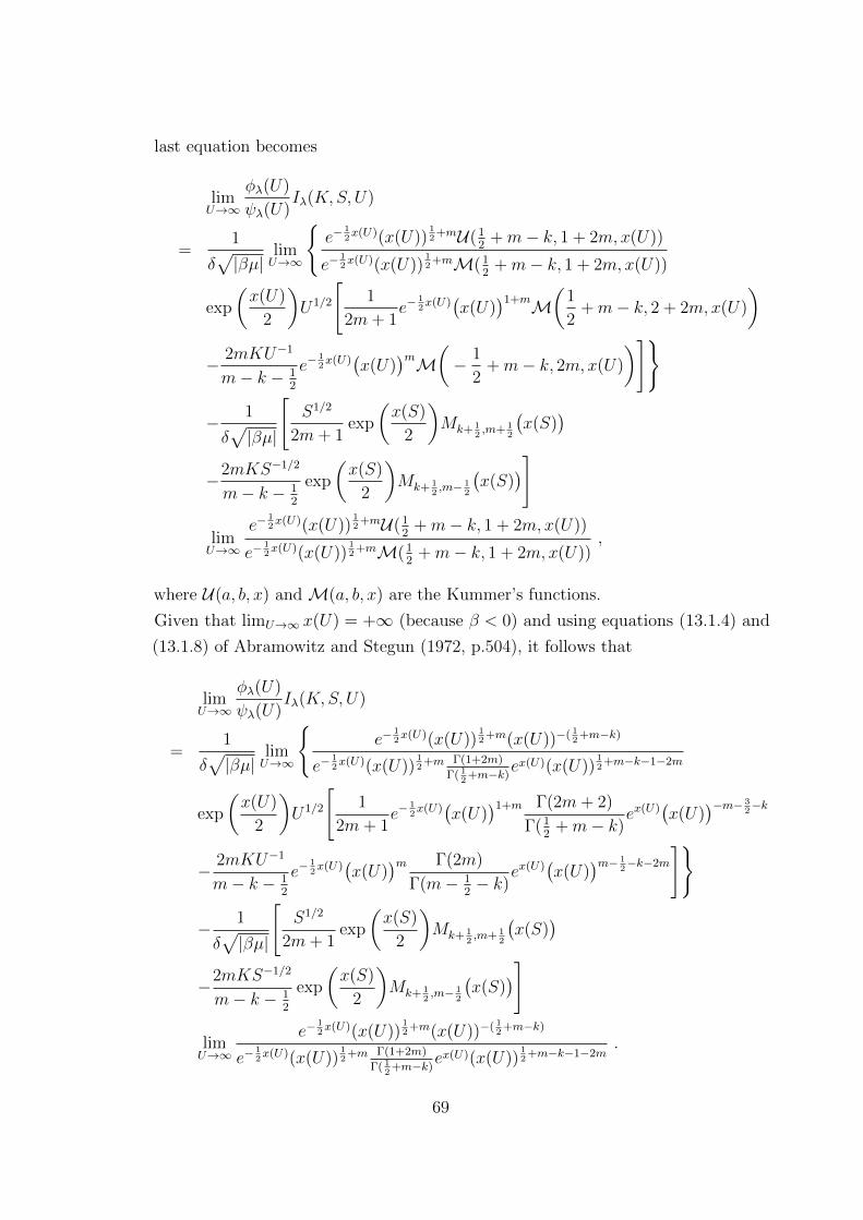
last equation becomes
limU→∞
φλ(U)
ψλ(U)Iλ(K,S, U)
=1
δ√|βµ|
limU→∞
e−
12x(U)(x(U))
12
+mU(12
+m− k, 1 + 2m,x(U))
e−12x(U)(x(U))
12
+mM(12
+m− k, 1 + 2m,x(U))
exp
(x(U)
2
)U1/2
[1
2m+ 1e−
12x(U)(x(U)
)1+mM(
1
2+m− k, 2 + 2m,x(U)
)
− 2mKU−1
m− k − 12
e−12x(U)(x(U)
)mM(− 1
2+m− k, 2m,x(U)
)]
− 1
δ√|βµ|
[S1/2
2m+ 1exp
(x(S)
2
)Mk+ 1
2,m+ 1
2
(x(S)
)−2mKS−1/2
m− k − 12
exp
(x(S)
2
)Mk+ 1
2,m− 1
2
(x(S)
)]
limU→∞
e−12x(U)(x(U))
12
+mU(12
+m− k, 1 + 2m,x(U))
e−12x(U)(x(U))
12
+mM(12
+m− k, 1 + 2m,x(U)),
where U(a, b, x) and M(a, b, x) are the Kummer’s functions.
Given that limU→∞ x(U) = +∞ (because β < 0) and using equations (13.1.4) and
(13.1.8) of Abramowitz and Stegun (1972, p.504), it follows that
limU→∞
φλ(U)
ψλ(U)Iλ(K,S, U)
=1
δ√|βµ|
limU→∞
e−
12x(U)(x(U))
12
+m(x(U))−( 12
+m−k)
e−12x(U)(x(U))
12
+m Γ(1+2m)
Γ( 12
+m−k)ex(U)(x(U))
12
+m−k−1−2m
exp
(x(U)
2
)U1/2
[1
2m+ 1e−
12x(U)(x(U)
)1+m Γ(2m+ 2)
Γ(12
+m− k)ex(U)
(x(U)
)−m− 32−k
− 2mKU−1
m− k − 12
e−12x(U)(x(U)
)m Γ(2m)
Γ(m− 12− k)
ex(U)(x(U)
)m− 12−k−2m
]
− 1
δ√|βµ|
[S1/2
2m+ 1exp
(x(S)
2
)Mk+ 1
2,m+ 1
2
(x(S)
)−2mKS−1/2
m− k − 12
exp
(x(S)
2
)Mk+ 1
2,m− 1
2
(x(S)
)]
limU→∞
e−12x(U)(x(U))
12
+m(x(U))−( 12
+m−k)
e−12x(U)(x(U))
12
+m Γ(1+2m)
Γ( 12
+m−k)ex(U)(x(U))
12
+m−k−1−2m.
69
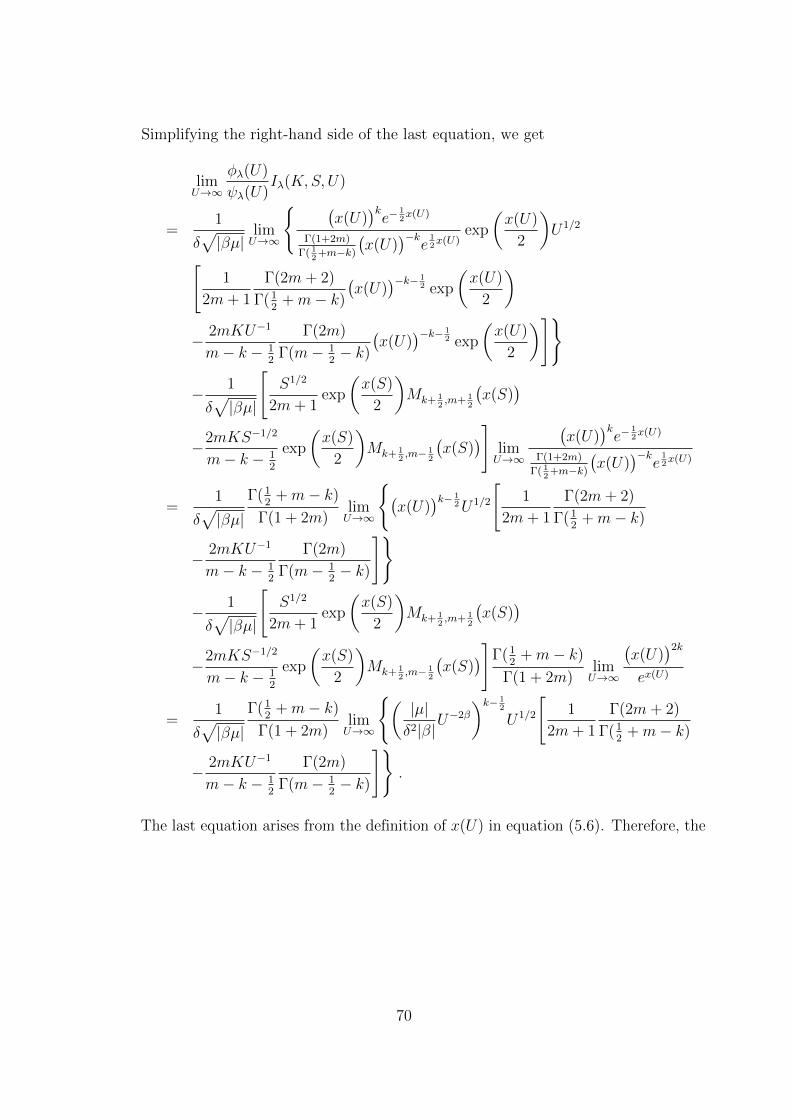
Simplifying the right-hand side of the last equation, we get
limU→∞
φλ(U)
ψλ(U)Iλ(K,S, U)
=1
δ√|βµ|
limU→∞
(x(U)
)ke−
12x(U)
Γ(1+2m)
Γ( 12
+m−k)
(x(U)
)−ke
12x(U)
exp
(x(U)
2
)U1/2
[1
2m+ 1
Γ(2m+ 2)
Γ(12
+m− k)
(x(U)
)−k− 12 exp
(x(U)
2
)
− 2mKU−1
m− k − 12
Γ(2m)
Γ(m− 12− k)
(x(U)
)−k− 12 exp
(x(U)
2
)]
− 1
δ√|βµ|
[S1/2
2m+ 1exp
(x(S)
2
)Mk+ 1
2,m+ 1
2
(x(S)
)−2mKS−1/2
m− k − 12
exp
(x(S)
2
)Mk+ 1
2,m− 1
2
(x(S)
)]limU→∞
(x(U)
)ke−
12x(U)
Γ(1+2m)
Γ( 12
+m−k)
(x(U)
)−ke
12x(U)
=1
δ√|βµ|
Γ(12
+m− k)
Γ(1 + 2m)limU→∞
(x(U)
)k− 12U1/2
[1
2m+ 1
Γ(2m+ 2)
Γ(12
+m− k)
− 2mKU−1
m− k − 12
Γ(2m)
Γ(m− 12− k)
]
− 1
δ√|βµ|
[S1/2
2m+ 1exp
(x(S)
2
)Mk+ 1
2,m+ 1
2
(x(S)
)−2mKS−1/2
m− k − 12
exp
(x(S)
2
)Mk+ 1
2,m− 1
2
(x(S)
)]Γ(12
+m− k)
Γ(1 + 2m)limU→∞
(x(U)
)2k
ex(U)
=1
δ√|βµ|
Γ(12
+m− k)
Γ(1 + 2m)limU→∞
(|µ|δ2|β|
U−2β
)k− 12
U1/2
[1
2m+ 1
Γ(2m+ 2)
Γ(12
+m− k)
− 2mKU−1
m− k − 12
Γ(2m)
Γ(m− 12− k)
].
The last equation arises from the definition of x(U) in equation (5.6). Therefore, the
70

last equation can be written as
limU→∞
φλ(U)
ψλ(U)Iλ(K,S, U)
=1
δ√|βµ|
Γ(12
+m− k)
Γ(1 + 2m)limU→∞
(|µ|δ2|β|
)k− 12
U−2β(k− 12
)+ 12
[1
2m+ 1
Γ(2m+ 2)
Γ(12
+m− k)
− 2mKU−1
m− k − 12
Γ(2m)
Γ(m− 12− k)
]. (E.1)
Assuming that λ > 0 is such that −2β(−12− 1
4β− λ
2|µβ| −12) + 1
2< 0, then equation
(E.1) is equal to zero.
For the integral Jλ(K,S, U), equation (5.15) yields:
limU→∞
Jλ(K,S, U)
= limU→∞
1
δ√|βµ|
[U1/2
k +m+ 12
exp
(x(U)
2
)Wk+ 1
2,m+ 1
2
(x(U)
)− KU−1/2
k −m+ 12
exp
(x(U)
2
)Wk+ 1
2,m− 1
2
(x(U)
)− S1/2
k +m+ 12
exp
(x(S)
2
)Wk+ 1
2,m+ 1
2
(x(S)
)+
KS−1/2
k −m+ 12
exp
(x(S)
2
)Wk+ 1
2,m− 1
2
(x(S)
)]
=1
δ√|βµ|
limU→∞
exp
(x(U)
2
)[U1/2
k +m+ 12
Wk+ 12,m+ 1
2
(x(U)
)− KU−1/2
k −m+ 12
Wk+ 12,m− 1
2
(x(U)
)]
− 1
δ√|βµ|
ex(S)2
[S1/2
k +m+ 12
Wk+ 12,m+ 1
2
(x(S)
)− KS−1/2
k −m+ 12
Wk+ 12,m− 1
2
(x(S)
)].
Using equation (13.1.33) of Abramowitz and Stegun (1972, p.505) the last equation
71

becomes
limU→∞
Jλ(K,S, U)
=1
δ√|βµ|
limU→∞
exp
(x(U)
2
)[U1/2
k +m+ 12
exp
(− x(U)
2
)(x(U)
)1+m
U(
1
2+m− k, 2 + 2m,x(U)
)− KU−1/2
k −m+ 12
exp
(− x(U)
2
)(x(U)
)mU(− 1
2+m− k, 2m,x(U)
)]
− 1
δ√|βµ|
ex(S)2
[S1/2
k +m+ 12
Wk+ 12,m+ 1
2
(x(S)
)− KS−1/2
k −m+ 12
Wk+ 12,m− 1
2
(x(S)
)],
where U(a, b, x) is the Kummer’s function.
Given that limU→∞ x(U) = +∞ (because β < 0) and using equation (13.1.8) of
Abramowitz and Stegun (1972, p.504), it follows that
limU→∞
Jλ(K,S, U)
=1
δ√|βµ|
limU→∞
U1/2
k +m+ 12
(x(U)
)1+m(x(U)
)− 12−m+k
− KU−1/2
k −m+ 12
(x(U)
)m(x(U)
) 12−m+k
]
− 1
δ√|βµ|
ex(S)2
[S1/2
k +m+ 12
Wk+ 12,m+ 1
2
(x(S)
)− KS−1/2
k −m+ 12
Wk+ 12,m− 1
2
(x(S)
)]
=1
δ√|βµ|
limU→∞
(x(U)
)k+ 12U1/2
[1
k +m+ 12
− KU−1
k −m+ 12
]
− 1
δ√|βµ|
ex(S)2
[S1/2
k +m+ 12
Wk+ 12,m+ 1
2
(x(S)
)− KS−1/2
k −m+ 12
Wk+ 12,m− 1
2
(x(S)
)]
=1
δ√|βµ|
limU→∞
(|µ|δ2|β|
U−2β
)k+ 12
U1/2
[1
k +m+ 12
− KU−1
k −m+ 12
]
− 1
δ√|βµ|
ex(S)2
[S1/2
k +m+ 12
Wk+ 12,m+ 1
2
(x(S)
)− KS−1/2
k −m+ 12
Wk+ 12,m− 1
2
(x(S)
)].
72

Simplifying the right-hand side of the last equation, we get
limU→∞
Jλ(K,S, U)
=1
δ√|βµ|
limU→∞
(|µ|δ2|β|
)k+ 12
U−2β(k+ 12
)+ 12
[1
k +m+ 12
− KU−1
k −m+ 12
]
− 1
δ√|βµ|
ex(S)2
[S1/2
k +m+ 12
Wk+ 12,m+ 1
2
(x(S)
)− KS−1/2
k −m+ 12
Wk+ 12,m− 1
2
(x(S)
)].
(E.2)
Using the definition of k provided in equation (5.10) the expression −2β(k + 12) + 1
2
can be written as
− 2β
(k +
1
2
)+
1
2= −2β
(− 1
2− 1
4β− λ
2|µβ|+
1
2
)+
1
2
=1
2− λ
|µ|+
1
2
= 1− λ
|µ|(E.3)
For λ > 0 large enough such that 1− λ|µ| < 0, equation (E.3) is negative and equation
(E.2) becomes
limU→∞
Jλ(K,S, U)
= − 1
δ√|βµ|
ex(S)2
[S1/2
k +m+ 12
Wk+ 12,m+ 1
2
(x(S)
)− KS−1/2
k −m+ 12
Wk+ 12,m− 1
2
(x(S)
)].
• If µ < 0 and β < 0, equations (5.4), (5.5) and (5.14) imply that
limU→∞
φλ(U)
ψλ(U)Iλ(K,S, U)
= limU→∞
Uβ+ 12 e
ε2x(U)Wk,m(x(U))
Uβ+ 12 e
ε2x(U)Mk,m(x(U))
1
δ√|βµ|
[U1/2
2m+ 1exp
(− x(U)
2
)Mk− 1
2,m+ 1
2
(x(U)
)+
2mKU−1/2
m+ k − 12
exp
(− x(U)
2
)Mk− 1
2,m− 1
2
(x(U)
)− S1/2
2m+ 1exp
(− x(S)
2
)Mk− 1
2,m+ 1
2
(x(S)
)−2mKS−1/2
m+ k − 12
exp
(− x(S)
2
)Mk− 1
2,m− 1
2
(x(S)
)],
73
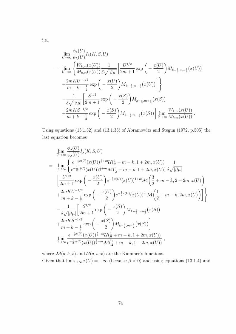
i.e.,
limU→∞
φλ(U)
ψλ(U)Iλ(K,S, U)
= limU→∞
Wk,m(x(U))
Mk,m(x(U))
1
δ√|βµ|
[U1/2
2m+ 1exp
(− x(U)
2
)Mk− 1
2,m+ 1
2
(x(U)
)+
2mKU−1/2
m+ k − 12
exp
(− x(U)
2
)Mk− 1
2,m− 1
2
(x(U)
)]
− 1
δ√|βµ|
[S1/2
2m+ 1exp
(− x(S)
2
)Mk− 1
2,m+ 1
2
(x(S)
)+
2mKS−1/2
m+ k − 12
exp
(− x(S)
2
)Mk− 1
2,m− 1
2
(x(S)
)]limU→∞
Wk,m(x(U))
Mk,m(x(U)).
Using equations (13.1.32) and (13.1.33) of Abramowitz and Stegun (1972, p.505) the
last equation becomes
limU→∞
φλ(U)
ψλ(U)Iλ(K,S, U)
= limU→∞
e−
12x(U)(x(U))
12
+mU(12
+m− k, 1 + 2m,x(U))
e−12x(U)(x(U))
12
+mM(12
+m− k, 1 + 2m,x(U))
1
δ√|βµ|[
U1/2
2m+ 1exp
(− x(U)
2
)e−
12x(U)(x(U))1+mM
(3
2+m− k, 2 + 2m,x(U)
)+
2mKU−1/2
m+ k − 12
exp
(− x(U)
2
)e−
12x(U)(x(U))mM
(1
2+m− k, 2m,x(U)
)]
− 1
δ√|βµ|
[S1/2
2m+ 1exp
(− x(S)
2
)Mk− 1
2,m+ 1
2
(x(S)
)+
2mKS−1/2
m+ k − 12
exp
(− x(S)
2
)Mk− 1
2,m− 1
2
(x(S)
)]limU→∞
e−12x(U)(x(U))
12
+mU(12
+m− k, 1 + 2m,x(U))
e−12x(U)(x(U))
12
+mM(12
+m− k, 1 + 2m,x(U)),
where M(a, b, x) and U(a, b, x) are the Kummer’s functions.
Given that limU→∞ x(U) = +∞ (because β < 0) and using equations (13.1.4) and
74

(13.1.8) of Abramowitz and Stegun (1972, p.504), it follows that
limU→∞
φλ(U)
ψλ(U)Iλ(K,S, U)
= limU→∞
e−
12x(U)(x(U))
12
+m(x(U))−12−m+k
e−12x(U)(x(U))
12
+m Γ(1+2m)
Γ( 12
+m−k)ex(U)(x(U))
12
+m−k−1−2m
1
δ√|βµ|[
U1/2
2m+ 1e−x(U)(x(U))1+m Γ(2 + 2m)
Γ(32
+m− k)ex(U)
(x(U)
) 32
+m−k−2−2m
+2mKU−1/2
m+ k − 12
e−x(U)(x(U))mΓ(2m)
Γ(12
+m− k)ex(U)
(x(U)
) 12
+m−k−2m]
− 1
δ√|βµ|
[S1/2
2m+ 1exp
(− x(S)
2
)Mk− 1
2,m+ 1
2
(x(S)
)+
2mKS−1/2
m+ k − 12
exp
(− x(S)
2
)Mk− 1
2,m− 1
2
(x(S)
)]limU→∞
e−12x(U)(x(U))
12
+m(x(U))−12−m+k
e−12x(U)(x(U))
12
+m Γ(1+2m)
Γ( 12
+m−k)ex(U)(x(U))
12
+m−k−1−2m
= limU→∞
Γ(1
2+m− k)
(x(U)
)ke−
x(U)2
Γ(1 + 2m)(x(U)
)−kex(U)2
1
δ√|βµ|[
U1/2
2m+ 1
Γ(2 + 2m)
Γ(32
+m− k)
(x(U)
)−k+ 12 +
2mKU−1/2
m+ k − 12
Γ(2m)
Γ(12
+m− k)
(x(U)
)−k+ 12
]
− 1
δ√|βµ|
[S1/2
2m+ 1exp
(− x(S)
2
)Mk− 1
2,m+ 1
2
(x(S)
)+
2mKS−1/2
m+ k − 12
exp
(− x(S)
2
)Mk− 1
2,m− 1
2
(x(S)
)]limU→∞
Γ(12
+m− k)(x(U)
)ke−
x(U)2
Γ(1 + 2m)(x(U)
)−kex(U)2
= limU→∞
Γ(1
2+m− k)
Γ(1 + 2m)
1
δ√|βµ|
(x(U)
)k+ 12 e−x(U)
[U1/2
2m+ 1
Γ(2 + 2m)
Γ(32
+m− k)
+2mKU−1/2
m+ k − 12
Γ(2m)
Γ(12
+m− k)
]
− 1
δ√|βµ|
[S1/2
2m+ 1exp
(− x(S)
2
)Mk− 1
2,m+ 1
2
(x(S)
)+
2mKS−1/2
m+ k − 12
exp
(− x(S)
2
)Mk− 1
2,m− 1
2
(x(S)
)]limU→∞
(Γ(1
2+m− k)
Γ(1 + 2m)
(x(U)
)2ke−x(U)
).
75

Using the definition of x(U) provided in equation (5.6), the last equation becomes
limU→∞
φλ(U)
ψλ(U)Iλ(K,S, U)
=Γ(1
2+m− k)
Γ(1 + 2m)
1
δ√|βµ|
limU→∞
(|µ|δ2|β|
U−2β
)k+ 12
e−x(U)U1/2
[1
2m+ 1
Γ(2 + 2m)
Γ(32
+m− k)+
2mKU−1
m+ k − 12
Γ(2m)
Γ(12
+m− k)
]=
Γ(12
+m− k)
Γ(1 + 2m)
1
δ√|βµ|
limU→∞
(|µ|δ2|β|
)k+ 12
e−x(U)U−2β(k+ 12
)+ 12[
1
2m+ 1
Γ(2 + 2m)
Γ(32
+m− k)+
2mKU−1
m+ k − 12
Γ(2m)
Γ(12
+m− k)
]. (E.4)
Using the definition of k provided in equation (5.10), the expression −2β(k + 12) + 1
2
can be written as
− 2β
(k +
1
2
)+
1
2= −2β
(1
2+
1
4β− λ
2|µβ|+
1
2
)+
1
2
= −2β − 1
2− λ
|µ|+
1
2
= −2β − λ
|µ|. (E.5)
Replacing equation (E.5) in equation (E.4), we get
limU→∞
φλ(U)
ψλ(U)Iλ(K,S, U)
=Γ(1
2+m− k)
Γ(1 + 2m)
1
δ√|βµ|
limU→∞
(|µ|δ2|β|
)k+ 12
e−x(U) δ2|β||µ|
|µ|δ2|β|
U−2βU−λ|µ|[
1
2m+ 1
Γ(2 + 2m)
Γ(32
+m− k)+
2mKU−1
m+ k − 12
Γ(2m)
Γ(12
+m− k)
]=
Γ(12
+m− k)
Γ(1 + 2m)
1
δ√|βµ|
limU→∞
(|µ|δ2|β|
)k+ 12 δ2|β||µ|
x(U)
ex(U)U−
λ|µ|[
1
2m+ 1
Γ(2 + 2m)
Γ(32
+m− k)+
2mKU−1
m+ k − 12
Γ(2m)
Γ(12
+m− k)
]= 0 .
76
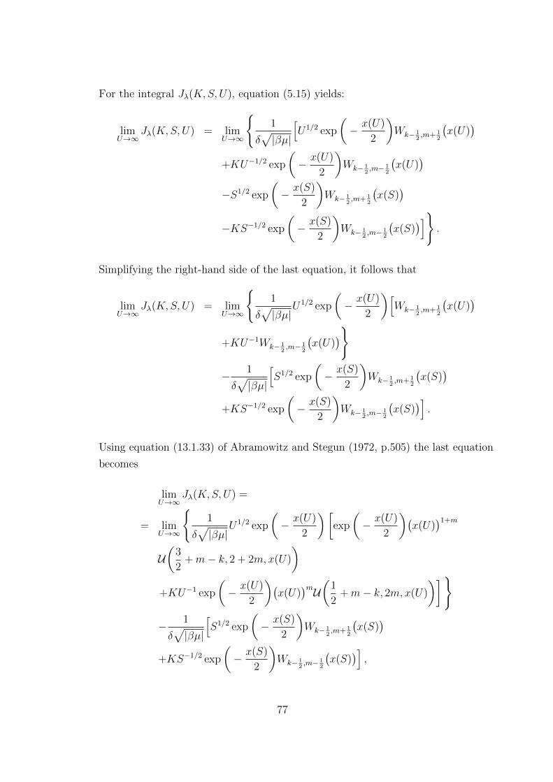
For the integral Jλ(K,S, U), equation (5.15) yields:
limU→∞
Jλ(K,S, U) = limU→∞
1
δ√|βµ|
[U1/2 exp
(− x(U)
2
)Wk− 1
2,m+ 1
2
(x(U)
)+KU−1/2 exp
(− x(U)
2
)Wk− 1
2,m− 1
2
(x(U)
)−S1/2 exp
(− x(S)
2
)Wk− 1
2,m+ 1
2
(x(S)
)−KS−1/2 exp
(− x(S)
2
)Wk− 1
2,m− 1
2
(x(S)
)].
Simplifying the right-hand side of the last equation, it follows that
limU→∞
Jλ(K,S, U) = limU→∞
1
δ√|βµ|
U1/2 exp
(− x(U)
2
)[Wk− 1
2,m+ 1
2
(x(U)
)+KU−1Wk− 1
2,m− 1
2
(x(U)
)
− 1
δ√|βµ|
[S1/2 exp
(− x(S)
2
)Wk− 1
2,m+ 1
2
(x(S)
)+KS−1/2 exp
(− x(S)
2
)Wk− 1
2,m− 1
2
(x(S)
)].
Using equation (13.1.33) of Abramowitz and Stegun (1972, p.505) the last equation
becomes
limU→∞
Jλ(K,S, U) =
= limU→∞
1
δ√|βµ|
U1/2 exp
(− x(U)
2
)[exp
(− x(U)
2
)(x(U)
)1+m
U(
3
2+m− k, 2 + 2m,x(U)
)+KU−1 exp
(− x(U)
2
)(x(U)
)mU(1
2+m− k, 2m,x(U)
)]
− 1
δ√|βµ|
[S1/2 exp
(− x(S)
2
)Wk− 1
2,m+ 1
2
(x(S)
)+KS−1/2 exp
(− x(S)
2
)Wk− 1
2,m− 1
2
(x(S)
)],
77

where U(a, b, x) is the Kummer’s function.
Given that limU→∞ x(U) = +∞ (because β < 0) and using equation (13.1.8) of
Abramowitz and Stegun (1972, p.504), we get
limU→∞
Jλ(K,S, U) = limU→∞
1
δ√|βµ|
U1/2e−x(U)[(x(U)
)1+m(x(U)
)− 32−m+k
+KU−1(x(U)
)m(x(U)
)− 12−m+k
− 1
δ√|βµ|
[S1/2 exp
(− x(S)
2
)Wk− 1
2,m+ 1
2
(x(S)
)+KS−1/2 exp
(− x(S)
2
)Wk− 1
2,m− 1
2
(x(S)
)]= lim
U→∞
1
δ√|βµ|
U1/2e−x(U)[(x(U)
)k− 12 +KU−1
(x(U)
)k− 12
− 1
δ√|βµ|
[S1/2 exp
(− x(S)
2
)Wk− 1
2,m+ 1
2
(x(S)
)+KS−1/2 exp
(− x(S)
2
)Wk− 1
2,m− 1
2
(x(S)
)]= lim
U→∞
1
δ√|βµ|
U1/2e−x(U)(x(U)
)k− 12
[1 +KU−1
]
− 1
δ√|βµ|
[S1/2 exp
(− x(S)
2
)Wk− 1
2,m+ 1
2
(x(S)
)+KS−1/2 exp
(− x(S)
2
)Wk− 1
2,m− 1
2
(x(S)
)].
Using the definition of x(U) provided in equation (5.6) the last equation becomes
limU→∞
Jλ(K,S, U) = limU→∞
1
δ√|βµ|
U1/2e−x(U)
(|µ|δ2|β|
U−2β
)k− 12[
1 +KU−1]
− 1
δ√|βµ|
[S1/2 exp
(− x(S)
2
)Wk− 1
2,m+ 1
2
(x(S)
)+KS−1/2 exp
(− x(S)
2
)Wk− 1
2,m− 1
2
(x(S)
)],
78

i.e.,
limU→∞
Jλ(K,S, U) = limU→∞
1
δ√|βµ|
U−2β(k− 12
)+ 12 e−x(U)
(|µ|δ2|β|
)k− 12 [
1 +KU−1]
− 1
δ√|βµ|
[S1/2 exp
(− x(S)
2
)Wk− 1
2,m+ 1
2
(x(S)
)+KS−1/2 exp
(− x(S)
2
)Wk− 1
2,m− 1
2
(x(S)
)]. (E.6)
Using the definition of k provided in equation (5.10) the expression −2β(k − 12) + 1
2
can be written as
− 2β
(k − 1
2
)+
1
2= −2β
(1
2+
1
4β− λ
2|µβ|− 1
2
)+
1
2
= −1
2− λ
|µ|+
1
2
= − λ
|µ|. (E.7)
Replacing equation (E.7) into equation (E.6), it follows that
limU→∞
Jλ(K,S, U) = limU→∞
1
δ√|βµ|
U−λ|µ| e−x(U)
(|µ|δ2|β|
)k− 12 [
1 +KU−1]
− 1
δ√|βµ|
[S1/2 exp
(− x(S)
2
)Wk− 1
2,m+ 1
2
(x(S)
)+KS−1/2 exp
(− x(S)
2
)Wk− 1
2,m− 1
2
(x(S)
)]= − 1
δ√|βµ|
[S1/2 exp
(− x(S)
2
)Wk− 1
2,m+ 1
2
(x(S)
)+KS−1/2 exp
(− x(S)
2
)Wk− 1
2,m− 1
2
(x(S)
)].
The last equation arises because λ > 0.
79

• If µ > 0 and β > 0, equations (5.4), (5.5) and (5.14) imply that
limU→∞
φλ(U)
ψλ(U)Iλ(K,S, U)
= limU→∞
Uβ+ 1
2 eε2x(U)Mk,m(x(U))
Uβ+ 12 e
ε2x(U)Wk,m(x(U))
1
δ√|βµ|[
U1/2 exp
(− x(U)
2
)Wk− 1
2,m− 1
2
(x(U)
)+KU−1/2 exp
(− x(U)
2
)Wk− 1
2,m+ 1
2
(x(U)
)−S1/2 exp
(− x(S)
2
)Wk− 1
2,m− 1
2
(x(S)
)−KS−1/2 exp
(− x(S)
2
)Wk− 1
2,m+ 1
2
(x(S)
)]=
1
δ√|βµ|
limU→∞
Mk,m(x(U))
Wk,m(x(U))exp
(− x(U)
2
)U1/2
[Wk− 1
2,m− 1
2
(x(U)
)+KU−1Wk− 1
2,m+ 1
2
(x(U)
)− 1
δ√|βµ|
[S1/2 exp
(− x(S)
2
)Wk− 1
2,m− 1
2
(x(S)
)+KS−1/2 exp
(− x(S)
2
)Wk− 1
2,m+ 1
2
(x(S)
)]limU→∞
Mk,m(x(U))
Wk,m(x(U)).
If β > 0 then limU→∞ x(U) = 0. Then, if we apply this result and equations (13.1.32)
80

and (13.1.33) of Abramowitz and Stegun (1972, p.505), the last equation becomes
limU→∞
φλ(U)
ψλ(U)Iλ(K,S, U)
=1
δ√|βµ|
limU→∞
e−
12x(U)(x(U)
) 12
+mM(
12
+m− k, 1 + 2m,x(U))
e−12x(U)(x(U)
) 12
+mU(
12
+m− k, 1 + 2m,x(U))
exp
(− x(U)
2
)U1/2
[exp
(− x(U)
2
)(x(U)
)mU(1
2+m− k, 2m,x(U)
)+KU−1 exp
(− x(U)
2
)(x(U)
)1+mU(
3
2+m− k, 2m+ 2, x(U)
)]
− 1
δ√|βµ|
[S1/2 exp
(− x(S)
2
)Wk− 1
2,m− 1
2
(x(S)
)+KS−1/2 exp
(− x(S)
2
)Wk− 1
2,m+ 1
2
(x(S)
)]limU→∞
e−12x(U)(x(U)
) 12
+mM(
12
+m− k, 1 + 2m,x(U))
e−12x(U)(x(U)
) 12
+mU(
12
+m− k, 1 + 2m,x(U)) ,
where M(a, b, x) and U(a, b, x) are the Kummer’s functions.
Simplifying the right-hand side of the last equation, it follows that
limU→∞
φλ(U)
ψλ(U)Iλ(K,S, U)
=1
δ√|βµ|
limU→∞
ex(U) limU→∞
M(12
+m− k, 1 + 2m,x(U))
U(
12
+m− k, 1 + 2m,x(U)) U1/2
[(x(U)
)mU(1
2+m− k, 2m,x(U)
)+KU−1
(x(U)
)1+mU(
3
2+m− k, 2m+ 2, x(U)
)]− 1
δ√|βµ|
[S1/2 exp
(− x(S)
2
)Wk− 1
2,m− 1
2
(x(S)
)+KS−1/2 exp
(− x(S)
2
)Wk− 1
2,m+ 1
2
(x(S)
)]limU→∞
M(
12
+m− k, 1 + 2m,x(U))
U(
12
+m− k, 1 + 2m,x(U)) .
81

i.e.,
limU→∞
φλ(U)
ψλ(U)Iλ(K,S, U)
=1
δ√|βµ|
limU→∞
M(12
+m− k, 1 + 2m,x(U))
U(
12
+m− k, 1 + 2m,x(U)) U1/2
[(x(U)
)mU(1
2+m− k, 2m,x(U)
)+KU−1
(x(U)
)1+mU(
3
2+m− k, 2m+ 2, x(U)
)]− 1
δ√|βµ|
[S1/2 exp
(− x(S)
2
)Wk− 1
2,m− 1
2
(x(S)
)+KS−1/2 exp
(− x(S)
2
)Wk− 1
2,m+ 1
2
(x(S)
)]limU→∞
M(
12
+m− k, 1 + 2m,x(U))
U(
12
+m− k, 1 + 2m,x(U)) .
(E.8)
Using equations (13.5.6)-(13.5.10) of Abramowitz and Stegun (1972, p.508) and
using the definition of m provided in equation (5.9), we can rewrite U(
12
+m−k, 1 +
2m,x(U))
, U(
12
+m− k, 2m,x(U))
and U(
32
+m− k, 2m+ 2, x(U))
as:
U(
1
2+m− k, 1 + 2m,x(U)
)
=
Γ(2m)
Γ( 12
+m−k)
(x(U)
)−2m+O(|x(U)|2m−1) ⇐ β < 1
2
Γ(1)Γ(1−k)
1x(U)
+O(| lnx(U)|) ⇐ β = 12
Γ(2m)
Γ( 12
+m−k)
(x(U)
)−2m+O(1) ⇐ β > 1
2
, (E.9)
U(
1
2+m− k, 2m,x(U)
)
=
Γ(2m−1)
Γ( 12
+m−k)
(x(U)
)1−2m+O(|x(U)|2m−2) ⇐ β < 1
4
Γ(1)
Γ( 32−k)
1x(U)
+O(| lnx(U)|) ⇐ β = 14
Γ(2m−1)
Γ( 12
+m−k)
(x(U)
)1−2m+O(1) ⇐ 1
4< β < 1
2
− 1Γ(1−k)
[ln(x(U)) + Ψ(1− k) + 2γ] +O(x(U) lnx(U)) ⇐ β = 12
Γ(1−2m)
Γ( 32−m−k)
+O(|x(U)|1−2m) ⇐ β > 12
,
(E.10)
82
and
U(
3
2+m− k, 2m+ 2, x(U)
)=
Γ(2m+ 1)
Γ(32
+m− k)
(x(U)
)−1−2m+O(|x(U)|2m) , (E.11)
where Ψ(x) is the logarithmic derivative of the gamma function and γ is the Euler’s
constant.
Replacing equations (E.9), (E.10) and (E.11) into equation (E.8), we get
I β < 14
limU→∞
φλ(U)
ψλ(U)Iλ(K,S, U)
=1
δ√|βµ|
limU→∞
M(12
+m− k, 1 + 2m,x(U))
Γ(2m)
Γ( 12
+m−k)
(x(U)
)−2m U1/2
[(x(U)
)m Γ(2m− 1)
Γ(12
+m− k)
(x(U)
)1−2m
+KU−1(x(U)
)1+m Γ(2m+ 1)
Γ(32
+m− k)
(x(U)
)−1−2m]
− 1
δ√|βµ|
[S1/2 exp
(− x(S)
2
)Wk− 1
2,m− 1
2
(x(S)
)+KS−1/2 exp
(− x(S)
2
)Wk− 1
2,m+ 1
2
(x(S)
)]limU→∞
M(
12
+m− k, 1 + 2m,x(U))
Γ(2m)
Γ( 12
+m−k)
(x(U)
)−2m
=1
δ√|βµ|
Γ(12
+m− k)
Γ(2m)limU→∞
M(
1
2+m− k, 1 + 2m,x(U)
)(x(U)
)2m
U1/2
[(x(U)
)1−m Γ(2m− 1)
Γ(12
+m− k)+KU−1
(x(U)
)−m Γ(2m+ 1)
Γ(32
+m− k)
]− 1
δ√|βµ|
[S1/2 exp
(− x(S)
2
)Wk− 1
2,m− 1
2
(x(S)
)+KS−1/2 exp
(− x(S)
2
)Wk− 1
2,m+ 1
2
(x(S)
)]limU→∞
M(
12
+m− k, 1 + 2m,x(U))
Γ(2m)
Γ( 12
+m−k)
(x(U)
)2m.
If β > 0 then limU→∞ x(U) = 0. Then, if we use this result and definition of
m in equation (5.9) and equation (13.5.5) of Abramowitz and Stegun (1972,
83

p.508), the last equation can be written as
limU→∞
φλ(U)
ψλ(U)Iλ(K,S, U)
=1
δ√|βµ|
Γ(12
+m− k)
Γ(2m)limU→∞
(x(U)
) 14|β|U1/2
[x(U)
Γ(2m− 1)
Γ(12
+m− k)+KU−1 Γ(2m+ 1)
Γ(32
+m− k)
].
Using the definition of x(U) provided in equation (5.6), the last equation
becomes
limU→∞
φλ(U)
ψλ(U)Iλ(K,S, U) =
=1
δ√|βµ|
Γ(12
+m− k)
Γ(2m)limU→∞
(|µ|δ2|β|
U−2β
) 14|β|
U1/2
[x(U)
Γ(2m− 1)
Γ(12
+m− k)+KU−1 Γ(2m+ 1)
Γ(32
+m− k)
]=
1
δ√|βµ|
Γ(12
+m− k)
Γ(2m)limU→∞
(|µ|δ2|β|
)m[x(U)
Γ(2m− 1)
Γ(12
+m− k)+KU−1 Γ(2m+ 1)
Γ(32
+m− k)
]= 0 . (E.12)
I β = 14
limU→∞
φλ(U)
ψλ(U)Iλ(K,S, U)
=1
δ√|βµ|
limU→∞
M(12
+ 1− k, 3, x(U))
Γ(2)
Γ( 12
+1−k)
(x(U)
)−2 U1/2
[x(U)
(Γ(1)
Γ(32− k)
1
x(U)+ | lnx(U)|
)+KU−1
(x(U)
)2 Γ(3)
Γ(32
+ 1− k)
(x(U)
)−3]
− 1
δ√|βµ|
[S1/2 exp
(− x(S)
2
)Wk− 1
2,1− 1
2
(x(S)
)+KS−1/2 exp
(− x(S)
2
)Wk− 1
2,1+ 1
2
(x(S)
)]limU→∞
M(
12
+ 1− k, 3, x(U))
Γ(2)
Γ( 12
+1−k)
(x(U)
)−2 ,
84
i.e.,
limU→∞
φλ(U)
ψλ(U)Iλ(K,S, U)
=1
δ√|βµ|
Γ(12
+ 1− k)
Γ(2)limU→∞
M(
1
2+ 1− k, 3, x(U)
)(x(U)
)2U1/2
[Γ(1)
Γ(32− k)
+ x(U)| lnx(U)|+KU−1(x(U)
)−1 Γ(3)
Γ(32
+ 1− k)
]− 1
δ√|βµ|
[S1/2 exp
(− x(S)
2
)Wk− 1
2,1− 1
2
(x(S)
)+KS−1/2 exp
(− x(S)
2
)Wk− 1
2,1+ 1
2
(x(S)
)]limU→∞
M(
12
+ 1− k, 3, x(U))
Γ(2)
Γ( 12
+1−k)
(x(U)
)2.
If β > 0 then limU→∞ x(U) = 0. Then, if we use this result and equation
(13.5.5) of Abramowitz and Stegun (1972, p.508), we get
limU→∞
φλ(U)
ψλ(U)Iλ(K,S, U)
=1
δ√|βµ|
Γ(12
+ 1− k)
Γ(2)limU→∞
(x(U)
)2U1/2
[Γ(1)
Γ(32− k)
+| lnx(U)|
1x(U)
+KU−1(x(U)
)−1 Γ(3)
Γ(32
+ 1− k)
].
Using the definition of x(U) provided in equation (5.6) as well as equation
(13.5.5) of Abramowitz and Stegun (1972, p.508), the last equation becomes
limU→∞
φλ(U)
ψλ(U)Iλ(K,S, U)
=1
δ√|βµ|
Γ(12
+ 1− k)
Γ(2)limU→∞
(|µ|δ2|β|
U−12
)2
U1/2
[Γ(1)
Γ(32− k)
+| lnx(U)|
1x(U)
+KU−1
(|µ|δ2|β|
U−12
)−1Γ(3)
Γ(32
+ 1− k)
]=
1
δ√|βµ|
Γ(12
+ 1− k)
Γ(2)limU→∞
(|µ|δ2|β|
)2
U−1/2
[Γ(1)
Γ(32− k)
+| lnx(U)|
1x(U)
+KU−1/2
(|µ|δ2|β|
)−1Γ(3)
Γ(32
+ 1− k)
].(E.13)
85

Equation (E.13) is equal to zero because limx→0| ln(x)|
1x
= 0 (this is easy to verify
using the L’Hospital’s rule).
I 14< β < 1
2
limU→∞
φλ(U)
ψλ(U)Iλ(K,S, U)
=1
δ√|βµ|
limU→∞
M(12
+m− k, 1 + 2m,x(U))
Γ(2m)
Γ( 12
+m−k)(x(U))−2m
U1/2
[(x(U)
)m( Γ(2m− 1)
Γ(12
+m− k)
(x(U)
)1−2m+ 1
)+KU−1
(x(U)
)1+m Γ(2m+ 1)
Γ(32
+m− k)
(x(U)
)−1−2m]
− 1
δ√|βµ|
[S1/2 exp
(− x(S)
2
)Wk− 1
2,m− 1
2
(x(S)
)+KS−1/2 exp
(− x(S)
2
)Wk− 1
2,m+ 1
2
(x(S)
)]limU→∞
M(
12
+m− k, 1 + 2m,x(U))
Γ(2m)
Γ( 12
+m−k)(x(U))−2m
Simplifying the right-hand side of the last equation, it follows that
limU→∞
φλ(U)
ψλ(U)Iλ(K,S, U)
=1
δ√|βµ|
limU→∞
M(12
+m− k, 1 + 2m,x(U))
Γ(2m)
Γ( 12
+m−k)
(x(U))2mU1/2
[Γ(2m− 1)
Γ(12
+m− k)
(x(U)
)1−m+(x(U)
)m+KU−1
(x(U)
)−m Γ(2m+ 1)
Γ(32
+m− k)
]− 1
δ√|βµ|
[S1/2 exp
(− x(S)
2
)Wk− 1
2,m− 1
2
(x(S)
)+KS−1/2 exp
(− x(S)
2
)Wk− 1
2,m+ 1
2
(x(S)
)]limU→∞
M(
12
+m− k, 1 + 2m,x(U))
Γ(2m)
Γ( 12
+m−k)
(x(U))2m .
Using equation (13.5.5) of Abramowitz and Stegun (1972, p.508) and using the
definitions of x(U) and m provided in equations (5.6) and (5.9), respectively,
86

the last equation becomes
limU→∞
φλ(U)
ψλ(U)Iλ(K,S, U)
=1
δ√|βµ|
Γ(12
+m− k)
Γ(2m)limU→∞
(|µ|δ2|β|
U−2β
)2m
U1/2
[Γ(2m− 1)
Γ(12
+m− k)
(x(U)
)1−m+(x(U)
)m+KU−1
(|µ|δ2|β|
U−2β
)−mΓ(2m+ 1)
Γ(32
+m− k)
]=
1
δ√|βµ|
Γ(12
+m− k)
Γ(2m)limU→∞
(|µ|δ2|β|
)2m
U−1/2
[Γ(2m− 1)
Γ(12
+m− k)
(x(U)
)1−m+(x(U)
)m+KU−1/2
(|µ|δ2|β|
)−mΓ(2m+ 1)
Γ(32
+m− k)
]= 0 . (E.14)
I β = 12
limU→∞
φλ(U)
ψλ(U)Iλ(K,S, U)
=1
δ√|βµ|
limU→∞
M(1− k, 2, x(U)
)Γ(1)
Γ(1−k)1
x(U)+ | lnx(U)|
U1/2
[(x(U)
) 12−1
Γ(1− k)
(ln(x(U)
)+ Ψ(1− k) + 2γ
)+KU−1
(x(U)
)1+ 12
Γ(2)
Γ(2− k)
(x(U)
)−2]
− 1
δ√|βµ|
[S1/2 exp
(− x(S)
2
)Wk− 1
2,0
(x(S)
)+KS−1/2 exp
(− x(S)
2
)Wk− 1
2,1
(x(S)
)]limU→∞
M(1− k, 2, x(U)
)Γ(1)
Γ(1−k)1
x(U)+ | lnx(U)|
.
87

Simplifying the right-hand side of last equation, we get
limU→∞
φλ(U)
ψλ(U)Iλ(K,S, U)
=1
δ√|βµ|
limU→∞
M(1− k, 2, x(U)
)Γ(1)
Γ(1−k)+ x(U)| lnx(U)|
U1/2x(U)[−1
Γ(1− k)
((x(U)
) 12 ln
(x(U)
)+(x(U)
) 12 Ψ(1− k) + 2γ
(x(U)
) 12
)+KU−1
(x(U)
)− 12
Γ(2)
Γ(2− k)
]− 1
δ√|βµ|
[S1/2 exp
(− x(S)
2
)Wk− 1
2,0
(x(S)
)+KS−1/2 exp
(− x(S)
2
)Wk− 1
2,1
(x(S)
)]limU→∞
M(1− k, 2, x(U)
)Γ(1)
Γ(1−k)+ | lnx(U)|
1x(U)
x(U) .
Using the equation (13.5.5) of Abramowitz and Stegun (1972, p.508) and the
definitions of x(U) and m, the last equation becomes
limU→∞
φλ(U)
ψλ(U)Iλ(K,S, U)
=1
δ√|βµ|
limU→∞
1
Γ(1)Γ(1−k)
+ x(U)| lnx(U)|U1/2 |µ|
δ2|β|U−1
[−1
Γ(1− k)
(ln(x(U)
)(x(U)
)− 12
+(x(U)
) 12 Ψ(1− k) + 2γ
(x(U)
) 12
)
+KU−1
(|µ|δ2|β|
U−1
)− 12 Γ(2)
Γ(2− k)
]=
1
δ√|βµ|
limU→∞
1
Γ(1)Γ(1−k)
+ x(U)| lnx(U)|U−1/2 |µ|
δ2|β|[1
Γ(1− k)
(− ln
(x(U)
)(x(U)
)− 12
−(x(U)
) 12 Ψ(1− k)− 2γ
(x(U)
) 12
)
+KU−1/2
(|µ|δ2|β|
)− 12 Γ(2)
Γ(2− k)
]= 0 . (E.15)
The last equation arises because limx→0− ln(x)(√x)−1 = 0 (this is easy to verify if we
apply the L’Hospital’s rule) and due to the fact that limU→0 x(U) = 0.
88

I β > 12
limU→∞
φλ(U)
ψλ(U)Iλ(K,S, U)
=1
δ√|βµ|
limU→∞
M(12
+m− k, 1 + 2m,x(U))
Γ(2m)
Γ( 12
+m−k)(x(U))−2m + 1
U1/2
[(x(U)
)m Γ(1− 2m)
Γ(32−m− k)
+KU−1(x(U)
)1+m Γ(2m+ 1)
Γ(32
+m− k)
(x(U)
)−1−2m]
− 1
δ√|βµ|
[S1/2 exp
(− x(S)
2
)Wk− 1
2,m− 1
2
(x(S)
)+KS−1/2 exp
(− x(S)
2
)Wk− 1
2,m+ 1
2
(x(S)
)]limU→∞
M(
12
+m− k, 1 + 2m,x(U))
Γ(2m)
Γ( 12
+m−k)(x(U))−2m + 1
=1
δ√|βµ|
limU→∞
M(12
+m− k, 1 + 2m,x(U))
Γ(2m)
Γ( 12
+m−k)+ (x(U))2m
(x(U)
)2mU1/2
[(x(U)
)m Γ(1− 2m)
Γ(32−m− k)
+KU−1(x(U)
)−m Γ(2m+ 1)
Γ(32
+m− k)
]− 1
δ√|βµ|
[S1/2 exp
(− x(S)
2
)Wk− 1
2,m− 1
2
(x(S)
)+KS−1/2 exp
(− x(S)
2
)Wk− 1
2,m+ 1
2
(x(S)
)]limU→∞
M(
12
+m− k, 1 + 2m,x(U))
Γ(2m)
Γ( 12
+m−k)+ (x(U))2m
(x(U)
)2m.
Using equation (13.5.5) of Abramowitz and Stegun (1972, p.508) and the
definitions of x(U) and m in equation (5.9), it follows that
limU→∞
φλ(U)
ψλ(U)Iλ(K,S, U)
=1
δ√|βµ|
limU→∞
1
Γ(2m)
Γ( 12
+m−k)+ (x(U))2m
(|µ|δ2|β|
U−2β
)2m
U1/2
[(x(U)
)m Γ(1− 2m)
Γ(32−m− k)
+KU−1
(|µ|δ2|β|
U−2β
)−mΓ(2m+ 1)
Γ(32
+m− k)
],
89
i.e.,
limU→∞
φλ(U)
ψλ(U)Iλ(K,S, U)
=1
δ√|βµ|
limU→∞
1
Γ(2m)
Γ( 12
+m−k)+ (x(U))2m
(|µ|δ2|β|
)2m
U−1/2
[(x(U)
)m Γ(1− 2m)
Γ(32−m− k)
+KU−1/2
(|µ|δ2|β|
)−mΓ(2m+ 1)
Γ(32
+m− k)
]= 0 . (E.16)
From equations (E.12) - (E.16) we conclude that
limU→∞
φλ(U)
ψλ(U)Iλ(K,S, U) = 0 , (E.17)
when µ > 0 and β > 0.
For the integral Jλ(K,S, U), equation (5.15) yields:
limU→∞
Jλ(K,S, U) = limU→∞
1
δ√|βµ|
[2mU1/2
k +m− 12
exp
(− x(U)
2
)Mk− 1
2,m− 1
2
(x(U)
)+KU−1/2
2m+ 1exp
(− x(U)
2
)Mk− 1
2,m+ 1
2
(x(U)
)− 2mS1/2
k +m− 12
exp
(− x(S)
2
)Mk− 1
2,m− 1
2
(x(S)
)−KS
−1/2
2m+ 1exp
(− x(S)
2
)Mk− 1
2,m+ 1
2
(x(S)
)]
=1
δ√|βµ|
limU→∞
2mU1/2
k +m− 12
exp
(− x(U)
2
)Mk− 1
2,m− 1
2
(x(U)
)+KU−1/2
2m+ 1exp
(− x(U)
2
)Mk− 1
2,m+ 1
2
(x(U)
)
− 1
δ√|βµ|
[2mS1/2
k +m− 12
exp
(− x(S)
2
)Mk− 1
2,m− 1
2
(x(S)
)+KS−1/2
2m+ 1exp
(− x(S)
2
)Mk− 1
2,m+ 1
2
(x(S)
)].
Using equation (13.1.32) of Abramowitz and Stegun (1972, p.505), the last equation
90

becomes
limU→∞
Jλ(K,S, U)
=1
δ√|βµ|
limU→∞
2mU1/2
k +m− 12
e−x(U)(x(U)
)mM(1
2+m− k, 2m,x(U)
)
+KU−1/2
2m+ 1e−x(U)
(x(U)
)1+mM(
3
2+m− k, 2 + 2m,x(U)
)
− 1
δ√|βµ|
[2mS1/2
k +m− 12
exp
(− x(S)
2
)Mk− 1
2,m− 1
2
(x(S)
)+KS−1/2
2m+ 1exp
(− x(S)
2
)Mk− 1
2,m+ 1
2
(x(S)
)]=
1
δ√|βµ|
limU→∞
e−x(U) limU→∞
2mU1/2
k +m− 12
(|µ|δ2|β|
U−2β
)mM(
1
2+m− k, 2m,x(U)
)
+1
δ√|βµ|
limU→∞
KU−1/2
2m+ 1e−x(U)
(x(U)
)1+mM(
3
2+m− k, 2 + 2m,x(U)
)
− 1
δ√|βµ|
[2mS1/2
k +m− 12
exp
(− x(S)
2
)Mk− 1
2,m− 1
2
(x(S)
)+KS−1/2
2m+ 1exp
(− x(S)
2
)Mk− 1
2,m+ 1
2
(x(S)
)],
where M(a, b, x) is the Kummer’s function. The last equation arises from the
definition of x(U) in equation (5.6).
If β > 0 then limU→∞ x(U) = 0. Using equation (13.5.5) of (Abramowitz and Stegun,
1972, p.508), it follows that
limU→∞
Jλ(K,S, U) =1
δ√|βµ|
limU→∞
2mU
12−2βm
k +m− 12
(|µ|δ2|β|
)m
− 1
δ√|βµ|
[2mS1/2
k +m− 12
exp
(− x(S)
2
)Mk− 1
2,m− 1
2
(x(S)
)+KS−1/2
2m+ 1exp
(− x(S)
2
)Mk− 1
2,m+ 1
2
(x(S)
)].
Using the definition of m provided in equation (5.9), the last equation can be written
91
as
limU→∞
Jλ(K,S, U) =1
δ√|βµ|
2m
k +m− 12
(|µ|δ2|β|
)m− 1
δ√|βµ|
[2mS1/2
k +m− 12
exp
(− x(S)
2
)Mk− 1
2,m− 1
2
(x(S)
)+KS−1/2
2m+ 1exp
(− x(S)
2
)Mk− 1
2,m+ 1
2
(x(S)
)].
• If µ < 0 and β > 0, equations (5.4), (5.5) and (5.14) imply that
limU→∞
φλ(U)
ψλ(U)Iλ(K,S, U)
= limU→∞
Uβ+ 1
2 eε2x(U)Mk,m(x(U))
Uβ+ 12 e
ε2x(U)Wk,m(x(U))
1
δ√|βµ|[
U1/2
k −m+ 12
exp
(x(U)
2
)Wk+ 1
2,m− 1
2
(x(U)
)− KU−1/2
m+ k + 12
exp
(x(U)
2
)Wk+ 1
2,m+ 1
2
(x(U)
)− S1/2
k −m+ 12
exp
(x(S)
2
)Wk+ 1
2,m− 1
2
(x(S)
)+
KS−1/2
m+ k + 12
exp
(x(S)
2
)Wk+ 1
2,m+ 1
2
(x(S)
)]=
1
δ√|βµ|
limU→∞
Mk,m(x(U))
Wk,m(x(U))
[U1/2
k −m+ 12
exp
(x(U)
2
)Wk+ 1
2,m− 1
2
(x(U)
)− KU−1/2
m+ k + 12
exp
(x(U)
2
)Wk+ 1
2,m+ 1
2
(x(U)
)]− 1
δ√|βµ|
[S1/2
k −m+ 12
exp
(x(S)
2
)Wk+ 1
2,m− 1
2
(x(S)
)− KS−1/2
m+ k + 12
exp
(x(S)
2
)Wk+ 1
2,m+ 1
2
(x(S)
)]limU→∞
Mk,m(x(U))
Wk,m(x(U)).
Using equations (13.1.32) and (13.1.33) of Abramowitz and Stegun (1972, p.505),
92

the last equation becomes
limU→∞
φλ(U)
ψλ(U)Iλ(K,S, U)
=1
δ√|βµ|
limU→∞
e−
12x(U)(x(U))
12
+mM(12
+m− k, 1 + 2m,x(U))
e−12x(U)(x(U))
12
+mU(12
+m− k, 1 + 2m,x(U))[U1/2
k −m+ 12
exp
(x(U)
2
)exp
(− x(U)
2
)(x(U)
)mU(m− k − 1
2, 2m,x(U)
)− KU−1/2
m+ k + 12
exp
(x(U)
2
)exp
(− x(U)
2
)(x(U)
)m+1
U(
1
2+m− k, 2 + 2m,x(U)
)]− 1
δ√|βµ|
[S1/2
k −m+ 12
exp
(x(S)
2
)Wk+ 1
2,m− 1
2
(x(S)
)− KS−1/2
m+ k + 12
exp
(x(S)
2
)Wk+ 1
2,m+ 1
2
(x(S)
)]limU→∞
e−12x(U)(x(U))
12
+mM(12
+m− k, 1 + 2m,x(U))
e−12x(U)(x(U))
12
+mU(12
+m− k, 1 + 2m,x(U))
=1
δ√|βµ|
limU→∞
M(12
+m− k, 1 + 2m,x(U))
U(12
+m− k, 1 + 2m,x(U))U1/2
(x(U)
)m[
1
k −m+ 12
U(m− k − 1
2, 2m,x(U)
)− KU−1
m+ k + 12
x(U)U(
1
2+m− k, 2 + 2m,x(U)
)]− 1
δ√|βµ|
[S1/2
k −m+ 12
exp
(x(S)
2
)Wk+ 1
2,m− 1
2
(x(S)
)− KS−1/2
m+ k + 12
exp
(x(S)
2
)Wk+ 1
2,m+ 1
2
(x(S)
)]limU→∞
M(12
+m− k, 1 + 2m,x(U))
U(12
+m− k, 1 + 2m,x(U)), (E.18)
where M(a, b, x) and U(a, b, x) are the Kummer’s functions.
Using equations (13.5.6) - (13.5.10) of Abramowitz and Stegun (1972, p.508) and the
definition of m in equation (5.9) and given that limU→∞ x(U) = 0, we can rewrite
U(m−k− 1
2, 2m,x(U)
), U(
12
+m−k, 2+2m,x(U))
and U(
12
+m−k, 1+2m,x(U))
93

as:
U(
1
2+m− k, 2m+ 2, x(U)
)=
Γ(2m+ 1)
Γ(12
+m− k)
(x(U)
)−1−2m+O(|x(U)|2m) , (E.19)
U(
1
2+m− k, 1 + 2m,x(U)
)
=
Γ(2m)
Γ( 12
+m−k)
(x(U)
)−2m+O(|x(U)|2m−1) ⇐ β < 1
2
Γ(1)Γ(1−k)
1x(U)
+O(| lnx(U)|) ⇐ β = 12
Γ(2m)
Γ( 12
+m−k)
(x(U)
)−2m+O(1) ⇐ β > 1
2
, (E.20)
U(m− k − 1
2, 2m,x(U)
)
=
Γ(2m−1)
Γ(m−k− 12
)
(x(U)
)1−2m+O(|x(U)|2m−2) ⇐ β < 1
4
Γ(1)
Γ( 12−k)
1x(U)
+O(| lnx(U)|) ⇐ β = 14
Γ(2m−1)
Γ(m−k− 12
)
(x(U)
)1−2m+O(1) ⇐ 1
4< β < 1
2
− 1Γ(−k)
[ln(x(U)) + Ψ(−k) + 2γ] +O(x(U) lnx(U)) ⇐ β = 12
Γ(1−2m)
Γ( 12−m−k)
+O(|x(U)|1−2m) ⇐ β > 12
,
(E.21)
where Ψ(x) is the logarithmic derivative of the gamma function and γ is the Euler’s
constant.
Replacing equations (E.19) - (E.21) into equation (E.18) and using equation (13.5.5)
of Abramowitz and Stegun (1972, p.508), we get (notice that limU→∞ x(U) = 0
because β > 0):
94
I β < 14
limU→∞
φλ(U)
ψλ(U)Iλ(K,S, U)
=1
δ√|βµ|
limU→∞
1
Γ(2m)
Γ( 12
+m−k)(x(U))−2m
U1/2(x(U)
)m[
1
k −m+ 12
Γ(2m− 1)
Γ(m− k − 12)
(x(U)
)1−2m
− KU−1
m+ k + 12
x(U)Γ(1 + 2m)
Γ(12
+m− k)
(x(U)
)−1−2m]
− 1
δ√|βµ|
[S1/2
k −m+ 12
exp
(x(S)
2
)Wk+ 1
2,m− 1
2
(x(S)
)− KS−1/2
m+ k + 12
exp
(x(S)
2
)Wk+ 1
2,m+ 1
2
(x(S)
)]limU→∞
1Γ(2m)
Γ( 12
+m−k)(x(U))−2m
.
Simplifying the right-hand side of the last equation, it follows that
limU→∞
φλ(U)
ψλ(U)Iλ(K,S, U)
=1
δ√|βµ|
Γ(12
+m− k)
Γ(2m)limU→∞
U1/2
(x(U)
)m[
1
k −m+ 12
Γ(2m− 1)
Γ(m− k − 12)x(U)− KU−1
m+ k + 12
Γ(1 + 2m)
Γ(12
+m− k)
].
Using the definitions of x(U) and m provided in equations (5.6) and (5.9),
respectively, the last equation becomes
limU→∞
φλ(U)
ψλ(U)Iλ(K,S, U)
=1
δ√|βµ|
Γ(12
+m− k)
Γ(2m)limU→∞
U1/2
(|µ|δ2|β|
U−2β
)m[
1
k −m+ 12
Γ(2m− 1)
Γ(m− k − 12)x(U)− KU−1
m+ k + 12
Γ(1 + 2m)
Γ(12
+m− k)
]=
1
δ√|βµ|
Γ(12
+m− k)
Γ(2m)limU→∞
(|µ|δ2|β|
)m[
1
k −m+ 12
Γ(2m− 1)
Γ(m− k − 12)x(U)− KU−1
m+ k + 12
Γ(1 + 2m)
Γ(12
+m− k)
]= 0 . (E.22)
95

I β = 14
limU→∞
φλ(U)
ψλ(U)Iλ(K,S, U)
=1
δ√|βµ|
limU→∞
1
Γ(2)
Γ( 32−k)
(x(U))−2U1/2x(U)
[1
k − 1 + 12
(Γ(1)
Γ(12− k)
1
x(U)+ | lnx(U)|
)− KU−1
1 + k + 12
x(U)Γ(3)
Γ(32− k)
(x(U)
)−3]
− 1
δ√|βµ|
[S1/2
k − 1 + 12
exp
(x(S)
2
)Wk+ 1
2,1− 1
2
(x(S)
)− KS−1/2
1 + k + 12
exp
(x(S)
2
)Wk+ 1
2,1+ 1
2
(x(S)
)]limU→∞
1Γ(2)
Γ( 32−k)
(x(U))−2.
Using the definition of x(U) provided in equation (5.6), the last equation can
be written as
limU→∞
φλ(U)
ψλ(U)Iλ(K,S, U)
=1
δ√|βµ|
limU→∞
1
Γ(2)
Γ( 32−k)
U1/2x(U)[1
k − 1 + 12
(Γ(1)
Γ(12− k)
x(U) +(x(U)
)2| lnx(U)|)− KU−1
1 + k + 12
Γ(3)
Γ(32− k)
]=
1
δ√|βµ|
limU→∞
1
Γ(2)
Γ( 32−k)
U1/2 |µ|δ2|β|
U−1/2
[1
k − 1 + 12
(Γ(1)
Γ(12− k)
x(U) +(x(U)
)2| lnx(U)|)− KU−1
1 + k + 12
Γ(3)
Γ(32− k)
]=
1
δ√|βµ|
1Γ(2)
Γ( 32−k)
|µ|δ2|β|
[1
k − 1 + 12
limU→∞
(Γ(1)
Γ(12− k)
x(U) +(x(U)
)2| lnx(U)|)− lim
U→∞
KU−1
1 + k + 12
Γ(3)
Γ(32− k)
]= 0 . (E.23)
The last equation arises because limU→∞ x(U) = 0 and limx→0 x2 lnx = 0
(aplying the L’Hospital’s rule).
96

I 14< β < 1
2
limU→∞
φλ(U)
ψλ(U)Iλ(K,S, U) =
=1
δ√|βµ|
limU→∞
1
Γ(2m)
Γ( 12
+m−k)
(x(U)
)−2mU1/2(x(U)
)m[
1
k −m+ 12
(Γ(2m− 1)
Γ(m− k − 12)
(x(U)
)1−2m+ 1
)− KU−1
m+ k + 12
x(U)Γ(1 + 2m)
Γ(12
+m− k)
(x(U)
)−1−2m]
− 1
δ√|βµ|
[S1/2
k −m+ 12
exp
(x(S)
2
)Wk+ 1
2,m− 1
2
(x(S)
)− KS−1/2
m+ k + 12
exp
(x(S)
2
)Wk+ 1
2,m+ 1
2
(x(S)
)]limU→∞
1Γ(2m)
Γ( 12
+m−k)
(x(U)
)−2m
=1
δ√|βµ|
limU→∞
1
Γ(2m)
Γ( 12
+m−k)
U1/2(x(U)
)m[
1
k −m+ 12
(Γ(2m− 1)
Γ(m− k − 12)x(U) +
(x(U)
)2m)
− KU−1
m+ k + 12
Γ(1 + 2m)
Γ(12
+m− k)
].
Using the definitions of x(U) and m provided in equations (5.6) and (5.9),
respectively, the last equation becomes
limU→∞
φλ(U)
ψλ(U)Iλ(K,S, U) =
1
δ√|βµ|
limU→∞
1
Γ(2m)
Γ( 12
+m−k)
U1/2
(|µ|δ2|β|
U−2β
)m[
1
k −m+ 12
(Γ(2m− 1)
Γ(m− k − 12)x(U) +
(x(U)
)2m)
− KU−1
m+ k + 12
Γ(1 + 2m)
Γ(12
+m− k)
]=
1
δ√|βµ|
limU→∞
1
Γ(2m)
Γ( 12
+m−k)
(|µ|δ2|β|
)m[
1
k −m+ 12
(Γ(2m− 1)
Γ(m− k − 12)x(U) +
(x(U)
)2m)
− KU−1
m+ k + 12
Γ(1 + 2m)
Γ(12
+m− k)
]= 0 . (E.24)
97

Equation (E.24) arises because limU→∞ x(U) = 0.
I β = 12
limU→∞
φλ(U)
ψλ(U)Iλ(K,S, U)
=1
δ√|βµ|
limU→∞
1
Γ(1)Γ(1−k)
1x(U)
+ | lnx(U)|U1/2
(x(U)
) 12
[1
k
(− 1
Γ(−k)
[ln(x(U)
)+ Ψ(−k) + 2γ
])−KU
−1
1 + kx(U)
Γ(2)
Γ(1− k)
(x(U)
)−2]
− 1
δ√|βµ|
[S1/2
kexp
(x(S)
2
)Wk+ 1
2,0
(x(S)
)−KS
−1/2
1 + kexp
(x(S)
2
)Wk+ 1
2,1
(x(S)
)]limU→∞
1Γ(1)
Γ(1−k)1
x(U)+ | lnx(U)|
=1
δ√|βµ|
limU→∞
1
Γ(1)Γ(1−k)
+ x(U)| lnx(U)|U1/2
(x(U)
) 32
[1
k
(− 1
Γ(−k)
[ln(x(U)
)+ Ψ(−k) + 2γ
])− KU−1
1 + k
(x(U)
)−1 Γ(2)
Γ(1− k)
].
Using the definitions of x(U) and m provided in equations (5.6) and (5.9),
respectively, it follows that
limU→∞
φλ(U)
ψλ(U)Iλ(K,S, U)
=1
δ√|βµ|
limU→∞
1
Γ(1)Γ(1−k)
+ x(U)| lnx(U)|U1/2
(|µ|δ2|β|
U−1
) 32
[1
k
(− 1
Γ(−k)
[ln(x(U)
)+ Ψ(−k) + 2γ
])−KU
−1
1 + k
(|µ|δ2|β|
U−1
)−1Γ(2)
Γ(1− k)
]=
1
δ√|βµ|
limU→∞
1
Γ(1)Γ(1−k)
+ x(U)| lnx(U)|
(|µ|δ2|β|
) 32
[1
k
(− U−1
Γ(−k)ln(x(U)
)− U−1
Γ(−k)[Ψ(−k) + 2γ]
)−KU
−1
1 + k
(|µ|δ2|β|
)−1Γ(2)
Γ(1− k)
].
98
Using again the definition of x(U), the last equation becomes
limU→∞
φλ(U)
ψλ(U)Iλ(K,S, U)
=1
δ√|βµ|
limU→∞
1
Γ(1)Γ(1−k)
+ | ln(x)|1
x(U)
(|µ|δ2|β|
) 32
[1
k
(− δ2|β|
Γ(−k)|µ|ln(x)
1x(U)
− U−1
Γ(−k)[Ψ(−k) + 2γ]
)−KU
−1
1 + k
(|µ|δ2|β|
)−1Γ(2)
Γ(1− k)
]= 0 . (E.25)
The last equation arises because limx→0| ln(x)|
1x(U)
= 0 and limx→0ln(x)
1x(U)
= 0 (these
are easy to verify using the L’Hospital Rule).
I β > 12
limU→∞
φλ(U)
ψλ(U)Iλ(K,S, U)
=1
δ√|βµ|
limU→∞
1
Γ(2m)
Γ( 12
+m−k)(x(U))−2m + 1
U1/2(x(U)
)m[
1
k −m+ 12
Γ(1− 2m)
Γ(12−m− k)
− KU−1
m+ k + 12
x(U)Γ(1 + 2m)
Γ(12
+m− k)
(x(U)
)−1−2m]
− 1
δ√|βµ|
[S1/2
k −m+ 12
exp
(x(S)
2
)Wk+ 1
2,m− 1
2
(x(S)
)− KS−1/2
m+ k + 12
exp
(x(S)
2
)Wk+ 1
2,m+ 1
2
(x(S)
)]limU→∞
1Γ(2m)
Γ( 12
+m−k)(x(U))−2m + 1
=1
δ√|βµ|
limU→∞
1
Γ(2m)
Γ( 12
+m−k)(x(U))−2m + 1
U1/2
(|µ|δ2|β|
U−2β
)m[
1
k −m+ 12
Γ(1− 2m)
Γ(12−m− k)
− KU−1
m+ k + 12
Γ(1 + 2m)
Γ(12
+m− k)
(|µ|δ2|β|
U−2β
)−2m].
99
The last equation arises from definition of x(U) provided in equation (5.6).
Using the definition of m given in equation (5.9), it follows that
limU→∞
φλ(U)
ψλ(U)Iλ(K,S, U)
=1
δ√|βµ|
limU→∞
1
Γ(2m)
Γ( 12
+m−k)(x(U))−2m + 1
(|µ|δ2|β|
)m[
1
k −m+ 12
Γ(1− 2m)
Γ(12−m− k)
− K
m+ k + 12
Γ(1 + 2m)
Γ(12
+m− k)
(|µ|δ2|β|
)−2m]= 0 . (E.26)
From equations (E.22) - (E.26) we conclude that
limU→∞
φλ(U)
ψλ(U)Iλ(K,S, U) = 0 , (E.27)
when µ < 0 and β > 0.
For the integral Jλ(K,S, U), and using equation (5.15)
limU→∞
Jλ(K,S, U)
= limU→∞
1
δ√|βµ|
[2mU1/2
k −m+ 12
exp
(x(U)
2
)Mk+ 1
2,m− 1
2
(x(U)
)+KU−1/2
2m+ 1exp
(x(U)
2
)Mk+ 1
2,m+ 1
2
(x(U)
)− 2mS1/2
k −m+ 12
exp
(x(S)
2
)Mk+ 1
2,m− 1
2
(x(S)
)−KS
−1/2
2m+ 1exp
(x(S)
2
)Mk+ 1
2,m+ 1
2
(x(S)
)]
=1
δ√|βµ|
limU→∞
2mU1/2
k −m+ 12
exp
(x(U)
2
)Mk+ 1
2,m− 1
2
(x(U)
)+KU−1/2
2m+ 1exp
(x(U)
2
)Mk+ 1
2,m+ 1
2
(x(U)
)
− 1
δ√|βµ|
[2mS1/2
k −m+ 12
exp
(x(S)
2
)Mk+ 1
2,m− 1
2
(x(S)
)+KS−1/2
2m+ 1exp
(x(S)
2
)Mk+ 1
2,m+ 1
2
(x(S)
)].
100

Using equation (13.1.32) of Abramowitz and Stegun (1972, p.505), we know that
Mk,m(z) = e−12zz
12
+mM(12
+ m − k, 1 + 2m, z), where M(a, b, x) is the Kummer’s
function. Then, the last equation becomes
limU→∞
Jλ(K,S, U)
=1
δ√|βµ|
limU→∞
2mU1/2
k −m+ 12
(x(U)
)mM(− 1
2+m− k, 2m,x(U)
)
+KU−1/2
2m+ 1
(x(U)
)1+mM(
1
2+m− k, 2 + 2m,x(U)
)
− 1
δ√|βµ|
[2mS1/2
k −m+ 12
exp
(x(S)
2
)Mk+ 1
2,m− 1
2
(x(S)
)+KS−1/2
2m+ 1exp
(x(S)
2
)Mk+ 1
2,m+ 1
2
(x(S)
)]=
1
δ√|βµ|
limU→∞
2mU1/2
k −m+ 12
(|µ|δ2|β|
U−2β
)mM(− 1
2+m− k, 2m,x(U)
)
+1
δ√|βµ|
limU→∞
KU−1/2
2m+ 1
(x(U)
)1+mM(
1
2+m− k, 2 + 2m,x(U)
)
− 1
δ√|βµ|
[2mS1/2
k −m+ 12
exp
(x(S)
2
)Mk+ 1
2,m− 1
2
(x(S)
)+KS−1/2
2m+ 1exp
(x(S)
2
)Mk+ 1
2,m+ 1
2
(x(S)
)].
The last equation arises from the definition of x(U) in equation (5.6).
If β > 0 then limU→∞ x(U) = 0. Using equation (13.5.5) of Abramowitz and Stegun
(1972, p.508), we get
limU→∞
Jλ(K,S, U) =1
δ√|βµ|
limU→∞
2mU
12−2βm
k −m+ 12
(|µ|δ2|β|
)m
− 1
δ√|βµ|
[2mS1/2
k −m+ 12
exp
(x(S)
2
)Mk+ 1
2,m− 1
2
(x(S)
)+KS−1/2
2m+ 1exp
(x(S)
2
)Mk+ 1
2,m+ 1
2
(x(S)
)].
Using the definition of m provided in equation (5.9) the exponent 12− 2βm is equal
101

to zero. Therefore, we get
limU→∞
Jλ(K,S, U) =1
δ√|βµ|
2m
k −m+ 12
(|µ|δ2|β|
)m− 1
δ√|βµ|
[2mS1/2
k −m+ 12
exp
(x(S)
2
)Mk+ 1
2,m− 1
2
(x(S)
)+KS−1/2
2m+ 1exp
(x(S)
2
)Mk+ 1
2,m+ 1
2
(x(S)
)].
• If µ = 0 and β < 0, equations (5.4), (5.5) and (5.14) yield:
limU→∞
φλ(U)
ψλ(U)Iλ(K,S, U)
= limU→∞
(U1/2Kν(
√2λz(U))
U1/2Iν(√
2λz(U))
2
δ√
2λ
[U1/2−βIν+1
(√2λz(U)
)−KU−1/2−βIν−1
(√2λz(U)
)− S1/2−βIν+1
(√2λz(S)
)+KS−1/2−βIν−1
(√2λz(S)
)])=
2
δ√
2λlimU→∞
(Kν(√
2λz(U))
Iν(√
2λz(U))
[U1/2−βIν+1
(√2λz(U)
)−KU−1/2−βIν−1
(√2λz(U)
)])− 2
δ√
2λ
[S1/2−βIν+1
(√2λz(S)
)−KS−1/2−βIν−1
(√2λz(S)
)]limU→∞
(Kν(√
2λz(U))
Iν(√
2λz(U))
).
Given that limU→∞ z(U) = +∞ (when β < 0) and using the asymptotic properties
of the modified Bessel functions (see Abramowitz and Stegun, 1972, p.377-378), the
102

last equation becomes
limU→∞
φλ(U)
ψλ(U)Iλ(K,S, U)
=2
δ√
2λlimU→∞
(√ π2√
2λz(U)e−√
2λz(U)
e√2λz(U)√
2π√
2λz(U)
[U1/2−β e
√2λz(U)√
2π√
2λz(U)
−KU−1/2−β e√
2λz(U)√2π√
2λz(U)
])− 2
δ√
2λ
[S1/2−βIν+1
(√2λz(S)
)
−KS−1/2−βIν−1
(√2λz(S)
)]limU→∞
√
π2√
2λz(U)e−√
2λz(U)
e√2λz(U)√
2π√
2λz(U)
=
2
δ√
2λlimU→∞
√
2π2√
2λz(U)√2√
2λz(U)e2√
2λz(U)
e√
2λz(U)√2π√
2λz(U)U1/2−β
[1−KU−1
]− 2
δ√
2λ
[S1/2−βIν+1
(√2λz(S)
)−KS−1/2−βIν−1
(√2λz(S)
)]limU→∞
√
2π2√
2λz(U)√2√
2λz(U)e2√
2λz(U)
=
2
δ√
2λ
√π
2√
2λlimU→∞
(U1/2−β√
z(U)e√
2λz(U)
)limU→∞
(1−KU−1
)− 2
δ√
2λ
[S1/2−βIν+1
(√2λz(S)
)−KS−1/2−βIν−1
(√2λz(S)
)]limU→∞
π
e2√
2λz(U).
Using the definition of z(U) provided in equation (5.7), the last equation becomes
limU→∞
φλ(U)
ψλ(U)Iλ(K,S, U)
=2
δ√
2λ
√π
2√
2λlimU→∞
U1/2−β√1δ|β|U
−β exp(√
2λ 1δ|β|U
−β)
=2
δ√
2λ
√π
2√
2λlimU→∞
U12−β
2√1δ|β| exp
(√2λ 1
δ|β|U−β) . (E.28)
To compute the limit in last equation, we have to apply the L’Hospital rule n times
103
such that β < − 12n−1
due to the fact that using n times the L’Hospital Rule, we get
limU→∞
U12−β
2√1δ|β| exp
(√2λ 1
δ|β|U−β) = lim
U→∞c
U12
+ 2n−12
β
exp(√
2λδ|β|U
−β) , (E.29)
where c is a constant (this is easy to verify using mathematical induction).
Therefore, if β < − 12n−1
then the exponent 12
+ 2n−12β is negative and the limit (E.29)
is zero.
Then equation (E.28) becomes
limU→∞
φλ(U)
ψλ(U)Iλ(K,S, U) = 0 .
For the integral Jλ(K,S, U), equation (5.15) yields:
limU→∞
Jλ(K,S, U)
=2
δ√
2λlimU→∞
[− U1/2−βKν+1
(√2λz(U)
)+KU−1/2−βKν−1
(√2λz(U)
)+S1/2−βKν+1
(√2λz(S)
)−KS−1/2−βKν−1
(√2λz(S)
)]=
2
δ√
2λlimU→∞
[− U1/2−β
√π
2√
2λz(U)e−√
2λz(U)
+KU−1/2−β√
π
2√
2λz(U)e−√
2λz(U)]
+2
δ√
2λ
(S1/2−βKν+1
(√2λz(S)
)−KS−1/2−βKν−1
(√2λz(S)
))=
2
δ√
2λ
√π
2√
2λlimU→∞
[√1
z(U)
U1/2−β
e√
2λz(U)
(− 1 +KU−1
)]
+2
δ√
2λ
(S1/2−βKν+1
(√2λz(S)
)−KS−1/2−βKν−1
(√2λz(S)
)).
The last equation arises if we apply equation (9.7.2) of Abramowitz and Stegun
(1972, p.378).
104

Using the definition of z(U) provided in equation (5.7), the last equation becomes
limU→∞
Jλ(K,S, U)
=2
δ√
2λ
√π
2√
2λlimU→∞
[√1
1δ|β|U
−βU1/2−β
exp(√
2λ 1δ|β|U
−β)
(− 1 +KU−1
)]
+2
δ√
2λ
(S1/2−βKν+1
(√2λz(S)
)−KS−1/2−βKν−1
(√2λz(S)
))=
2
δ√
2λ
√π
2√
2λlimU→∞
[U
12−β
2√1δ|β| exp(
√2λ 1
δ|β|U−β)
(− 1 +KU−1
)]
+2
δ√
2λ
(S1/2−βKν+1
(√2λz(S)
)−KS−1/2−βKν−1
(√2λz(S)
))=
2
δ√
2λ
(S1/2−βKν+1
(√2λz(S)
)−KS−1/2−βKν−1
(√2λz(S)
)). (E.30)
The last equation arises using the same arguments used in equation (E.29).
• If µ = 0 and β > 0, equations (5.4), (5.5) and (5.14) yield:
limU→∞
φλ(U)
ψλ(U)Iλ(K,S, U)
= limU→∞
(U1/2Iν(
√2λz(U))
U1/2Kν(√
2λz(U))
2
δ√
2λ
[U1/2−βKν−1
(√2λz(U)
)−KU−1/2−βKν+1
(√2λz(U)
)− S1/2−βKν−1
(√2λz(S)
)+KS−1/2−βKν+1
(√2λz(S)
)])=
2
δ√
2λlimU→∞
(Iν(√
2λz(U))
Kν(√
2λz(U))
[U1/2−βKν−1
(√2λz(U)
)−KU−1/2−βKν+1
(√2λz(U)
)])− 2
δ√
2λ
[S1/2−βKν−1
(√2λz(S)
)−KS−1/2−βKν+1
(√2λz(S)
)]limU→∞
(Iν(√
2λz(U))
Kν(√
2λz(U))
).
Given that limU→∞ z(U) = 0 (when β > 0) and using the limiting forms for small
arguments of the modified Bessel functions (see Abramowitz and Stegun, 1972,
105
p.375), the last equation becomes
limU→∞
φλ(U)
ψλ(U)Iλ(K,S, U)
=2
δ√
2λlimU→∞
( ( 12
√2λz(U))ν
Γ(ν+1)
12Γ(ν)(1
2
√2λz(U))−ν
[U1/2−β 1
2Γ(ν − 1)
(1
2
√2λz(U)
)−ν+1
−KU−1/2−β 1
2Γ(ν + 1)
(1
2
√2λz(U)
)−ν−1])− 2
δ√
2λ
[S1/2−βKν−1
(√2λz(S)
)−KS−1/2−βKν+1
(√2λz(S)
)]limU→∞
( ( 12
√2λz(U))ν
Γ(ν+1)
12Γ(ν)(1
2
√2λz(U))−ν
)
=4
δ√
2λΓ(ν)Γ(ν + 1)limU→∞
((1
2
√2λz(U)
)2ν1
2U1/2−β
(1
2
√2λz(U)
)−ν−1
[Γ(ν − 1)
(1
2
√2λz(U)
)2
−KU−1Γ(ν + 1)
])− 4
δ√
2λΓ(ν)Γ(ν + 1)
[S1/2−βKν−1
(√2λz(S)
)−KS−1/2−βKν+1
(√2λz(S)
)]limU→∞
(1
2
√2λz(U)
)2ν
.
Using the definitions of z(U) and ν provided in equations (5.7) and (5.11), respec-
tively, it follows that
limU→∞
φλ(U)
ψλ(U)Iλ(K,S, U)
=2
δ√
2λΓ(ν)Γ(ν + 1)limU→∞
((1
2
√2λ
1
δ|β|U−β
) 12|β|−1
U1/2−β
[Γ(ν − 1)
(1
2
√2λ
1
δ|β|U−β
)2
−KU−1Γ(ν + 1)
])
=2
δ√
2λΓ(ν)Γ(ν + 1)
(1
2
√2λ
1
δ|β|
) 12|β|−1
limU→∞
(Γ(ν − 1)
(1
2
√2λ
1
δ|β|U−β
)2
−KU−1Γ(ν + 1)
)= 0 .
106
For the integral Jλ(K,S, U), and using equation (5.15), we have
limU→∞
Jλ(K,S, U)
=2
δ√
2λlimU→∞
[− U1/2−βIν−1
(√2λz(U)
)+KU−1/2−βIν+1
(√2λz(U)
)+S1/2−βIν−1
(√2λz(S)
)−KS−1/2−βIν+1
(√2λz(S)
)]. (E.31)
Using equation (9.6.7) of Abramowitz and Stegun (1972, p.375), we get
limU→∞
Jλ(K,S, U)
=2
δ√
2λlimU→∞
[− U1/2−β (1
2
√2λz(U))ν−1
Γ(ν)+KU−1/2−β (1
2
√2λz(U))ν+1
Γ(ν + 2)
]+
2
δ√
2λ
(S1/2−βIν−1
(√2λz(S)
)−KS−1/2−βIν+1
(√2λz(S)
))=
2
δ√
2λlimU→∞
[U−1/2−β
(− U
(12
√2λz(U))ν−1
Γ(ν)+K
(12
√2λz(U))ν+1
Γ(ν + 2)
)]
+2
δ√
2λ
(S1/2−βIν−1
(√2λz(S)
)−KS−1/2−βIν+1
(√2λz(S)
)).
Using the definitions of z(U) and ν provided in equations (5.7) and (5.11), respec-
tively, the last equation becomes
limU→∞
Jλ(K,S, U)
=2
δ√
2λlimU→∞
[U−1/2−β
(− U
(12
√2λ 1
δ|β|U−β)
12|β|−1
Γ(ν)+K
(12
√2λz(U))ν+1
Γ(ν + 2)
)]
+2
δ√
2λ
(S1/2−βIν−1
(√2λz(S)
)−KS−1/2−βIν+1
(√2λz(S)
))
=2
δ√
2λlimU→∞
[(12
√2λ 1
δ|β|
)ν−1
Γ(ν)+KU−1/2−β
(12
√2λz(U)
)ν+1
Γ(ν + 2)
]
+2
δ√
2λ
(S1/2−βIν−1
(√2λz(S)
)−KS−1/2−βIν+1
(√2λz(S)
))=
2
δ√
2λ
[1
Γ(ν)
(√2λ
2δ|β|
)ν−1
+ S1/2−βIν−1
(√2λz(S)
)−KS−1/2−βIν+1
(√2λz(S)
)]. (E.32)
107
Bibliography
Abate, J. and W. Whitt, 1995, Numerical Inversion of Laplace Transforms of Probability
Distributions, ORSA Journal on Computing 7, 36--43.
Abramowitz, M. and I. Stegun, 1972, Handbook of Mathematical Functions (Dover
Publications, New York).
Babbs, S., 2000, Binomial valuation of lookback options, Journal of Economic Dynamics
& Control 24, 1499--1525.
Bekaert, G. and G. Wu, 2000, Asymmetric Volatility and Risk in Equity Markets, Review
of Financial Studies 13, 1--42.
Benson, R. and N. Daniel, 1991, Up, Over and Out, Risk 4.
Bermin, H., 2000, Hedging lookback and partial lookback options using Malliavin calculus,
Applied Mathematical Finance 7, 75--100.
Black, F. and M. Scholes, 1973, The Pricing of Options and Corporate Liabilities, Journal
of Political Economy 81, 637--654.
Borodin, A. and P. Salminen, 1996, Handbook of Brownian Motion - Facts and Formulae,
Probability and Its Applications (Birkhauser Verlag, Basel).
Boyle, P. and S. Lau, 1994, Bumping up against the Barrier with the Bumping up against
the Barrier with the Binomial Method, Journal of Derivatives.
Boyle, P. and Y. Tian, 1999, Pricing Lookback and Barrier Options under the CEV
Process, Journal of Financial and Quantitative Analysis 34, 241--264.
Cheuk, T. and T. Vorst, 1997, Currency lookback options and observation frequency: a
binomial approach, Journal of International Money and Finance 16, 173--187.
Conze, A. and R. Viswanathan, 1991, Path-dependent options: The case of lookback
options, Journal of Finance 46, 1893--1907.
108
Cox, J., 1975, Notes on Option Pricing I: Constant Elasticity of Variance Diffusions,
Working paper, Stanford University (reprinted in Journal of Portfolio Management,
1996, December, 15-17).
Cox, J. and S. Ross, 1976, The Valuation of Options for Alternative Stochastic Processes,
Journal of Financial Economics 3, 145--166.
Cox, J., S. Ross, and M. Rubinstein, 1979, Option Pricing: A Simplified Approach, Journal
of Financial Economics 7, 229--263.
Davydov, D. and V. Linetsky, 2001, Pricing and Hedging Path-Dependent Options Under
the CEV Process, Management Science 47, 949--965.
Davydov, D. and V. Linetsky, 2003, Pricing Options on Scalar Diffusions: An Eigenfunction
Expansion Approach, Operations Research 51, 185--209.
Dennis, P. and S. Mayhew, 2002, Risk-Neutral Skewness: Evidence from Stock Options,
Journal of Financial and Quantitative Analysis 37, 471--493.
Duffie, D., 1996, Swap Rates and Credit Quality, Journal of Finance 51, 921--949.
Emanuel, D. and J. MacBeth, 1982, Further Results on the Constant Elasticity of Variance
Call Option Pricing Model, Journal of Financial and Quantitative Analysis 17, 533--554.
Eriksson, Jonatan, 2006, Explicit Pricing Formulas for Turbo Warrants, Risk Magazine.
Eriksson, Jonatan and Jonas Persson, 2006, Pricing Turbo Warrants, Working paper,
Swedish Graduate School in Mathematics and Computing.
Faulhaber, O., Analytic Methods for Pricing Double Barrier Options in the Presence of
Stochastic Volatility, Master’s thesis, University of Kaiserslautern 2002.
Ferreira, S., Barrier options under the CEV diffusion, Master’s thesis, ISCTE and FCUL
2009.
Geman, H. and M. Yor, 1996, Pricing and Hedging Double Barrier Options: A Probabilistic
Approach, Mathematical Finance 6, 365--378.
Goldman, M., H. Sosin, and L. Shepp, 1979a, On contingent claims that insure ex-post
optimal stock market timing, Journal of Finance 34, 401--413.
Goldman, M., H. Sosin, and M. Gatto, 1979b, Path-dependent options, Journal of Finance
34, 1111--1127.
109

Griebsch, S. and U. Wystup, 2008, On the Valuation of Fader and Discrete Barrier Options
in Heston’s Stochastic Volatility Model, Working paper, Frankfurt School of Finance &
Management.
Heston, S., 1993, A Closed-Form Solution for Options with Stochastic Volatility with
Applications to Bond and Currency Options, Review of Financial Studies 6, 327--343.
Hudson, M., 1991, The Value in Going Out, Risk 4, 29 -- 33.
Hull, J., 2002, Options, Futures and Other Derivatives, fifth ed. (Prentice-Hall).
Jackwerth, J. and M. Rubinstein, 2001, Recovering Stochastic Processes from Option
Prices, Working paper, University of Konstanz and Haas School of Business.
Kuan, G. and N. Webber, 2003, Pricing Barrier Options with One-Factor Interest Rate
Models, Journal of Derivatives 10, 33--50.
Kunitomo, N. and M. Ikeda, 1992, Pricing Options with Curved Boundaries, Mathematical
Finance 2, 275--298.
Linetsky, V., 2004, Lookback options and diffusion hitting times: A spectral expansion
approach, Finance and Stochastics 8, 373--398.
Lipton, A., 2001, Mathematical Methods for Foreign Exchange, first ed. (World Scientific,
London).
Lo, C. F. and C. H. Hui, 2007, Valuing double barrier options with time-dependent
parameters by Fourier series expansion, IAENG International Journal of Applied
Mathematics 36.
Lo, C. F., H. Tang, K. C. Ku, and C. H. Hui, 2009, Valuing Time-Dependent CEV Barrier
Options, Journal of Applied Mathematics and Decision Sciences.
MacBeth, J. and L. Merville, 1980, Tests of the Black-Scholes and Cox Call Option
Valuation Models, Journal of Finance, 285--301.
Merton, R., 1973, The Theory of Rational Option Pricing, Bell Journal of Economics and
Management Science 4, 141--183.
Mijatovic, A., 2010, Local Time and the Pricing of Time-Dependent Barrier Options,
Finance and Stochastics 14, 13--48.
110
Nunes, J. and J. Dias, 2011, The Valuation of Double Barrier Options under Multifactor
Pricing Models, Working paper, BRU-UNIDE and ISCTE-IUL Business School.
Pelsser, A., 2000, Pricing Double Barrier Options Using Laplace Transforms, Finance and
Stochastics 4, 95--104.
Rubinstein, M. and E. Reiner, 1991, Breaking Down the Barriers, Risk 4, 28--35.
Schmalensee, R. and R. Trippi, 1978, Common Stock Volatility Expectations Implied by
Option Premia, Journal of Finance 33, 129--147.
Schroder, M., 2000, On the valuation of double-barrier options: Computational aspects,
Journal of Computational Finance 3.
Snyder, Gerard L., 1969, Alternative Forms of Options, Financial Analysts Journal 25,
93--99.
Wong, Hoi Ying and Chun Man Chan, 2008, Turbo Warrants under Stochastic Volatility,
Quantitative Financetive 8, 739--751.
Wong, Hoi Ying and Ka Yung Lau, 2008, Analytical Valuation of Turbo Warrants under
Double Exponential Jump Diffusion, Journal of Derivatives 15, 61--73.
Xu, C. and Y. Kwok, 2005, Integral Price Formulas for Lookback Options, Journal of
Applied Mathematics, 117--125.
Zhang, P., 1998, Exotic Options: A Guide to Second Generation Options, second ed.
(World Scientific, Singapore).
111