1

Gas Lift WorkshopGas Lift WorkshopDoha Doha –– QatarQatar

44--8 February 20078 February 2007

The Use of Dynamic SimulationThe Use of Dynamic SimulationTechniques in Gas Lift OptimisationTechniques in Gas Lift Optimisation

by Juan Carlos Mantecon

2

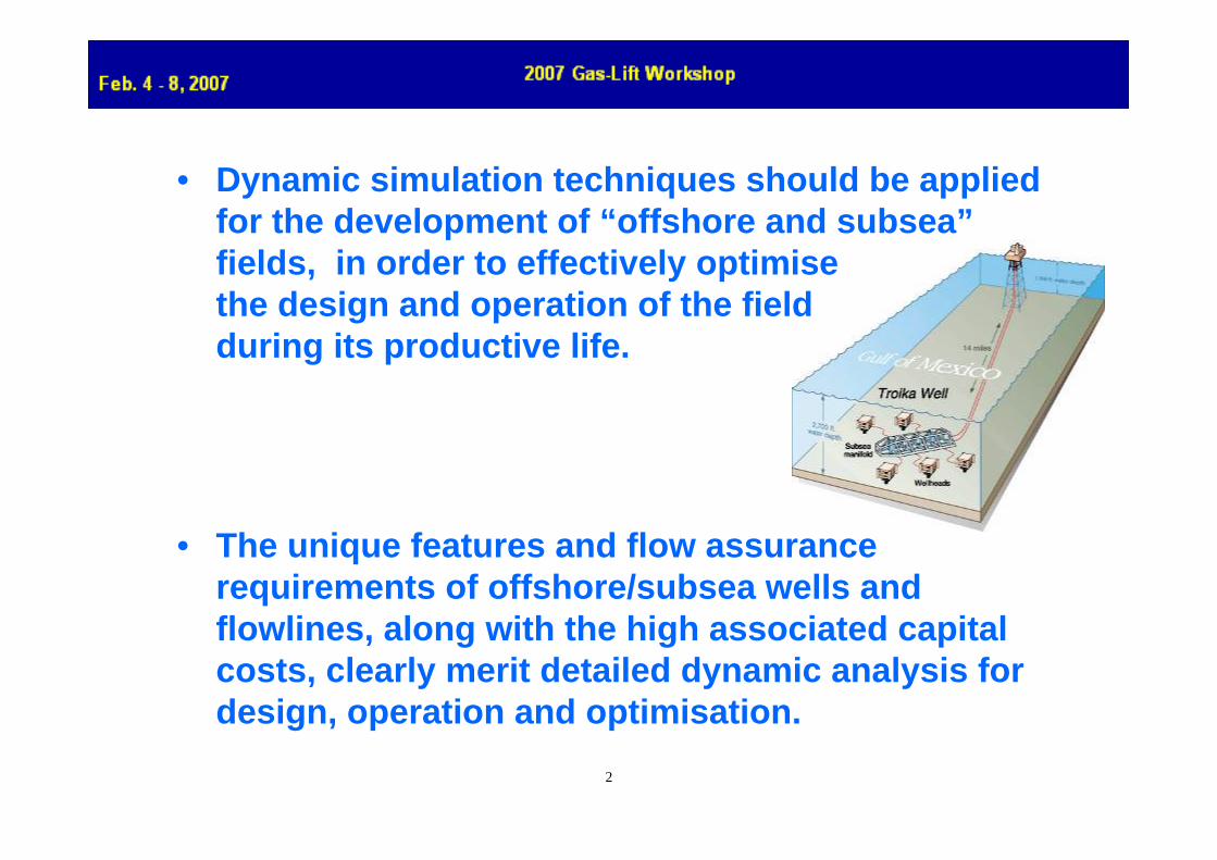
• Dynamic simulation techniques should be applied for the development of “offshore and subsea”fields, in order to effectively optimise the design and operation of the field during its productive life.

• The unique features and flow assurance requirements of offshore/subsea wells and flowlines, along with the high associated capital costs, clearly merit detailed dynamic analysis for design, operation and optimisation.

3

• Dynamic simulations provide valuable information for savings and reduction of potential problems (risk reduction) during well completions and production system kick-off operations.

• The knowledge of the minimum flow rates required to clean up the wells will have relevant implications on test equipment selection (size) and therefore cost minimisation.

• Furthermore, the ability to predict (what if cases) and be prepared to deal with potential problems (or GL need) not only can save millions of dollars but can minimise any environmental impact.

4

Dynamic Simulation

5

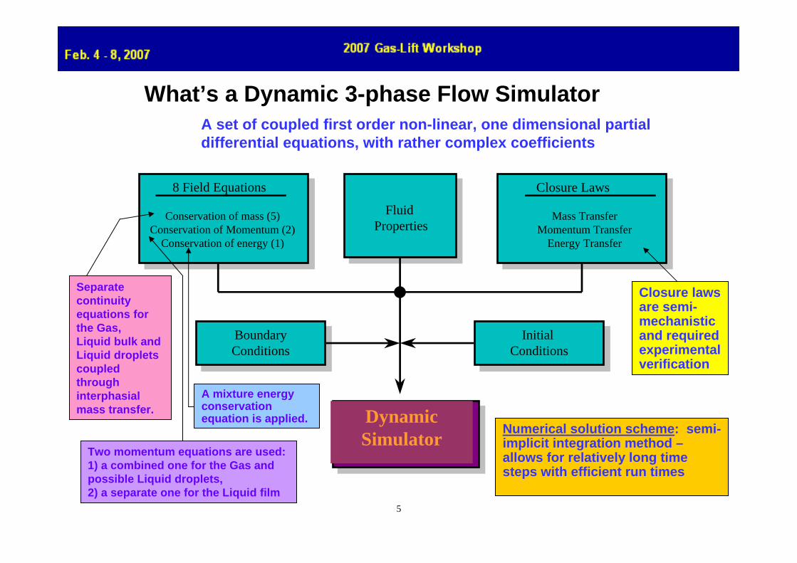
What’s a Dynamic 3-phase Flow Simulator

8 Field Equations

Fluid Properties

Conservation of mass (5)Conservation of Momentum (2)

Conservation of energy (1)

Closure Laws

Mass TransferMomentum Transfer

Energy Transfer

BoundaryConditions

Initial Conditions

A set of coupled first order non-linear, one dimensional partial differential equations, with rather complex coefficients

Numerical solution scheme: semi-implicit integration method –allows for relatively long time steps with efficient run times

Closure laws are semi-mechanistic and required experimental verification

Two momentum equations are used: 1) a combined one for the Gas and possible Liquid droplets, 2) a separate one for the Liquid film

Separate continuity equations for the Gas, Liquid bulk andLiquid dropletscoupled through interphasialmass transfer.

A mixture energy conservation equation is applied. Dynamic

Simulator

6

OLGA - Dynamic 3-phase Flow Simulator

• OLGA model has been tested against experimental data over a substancial range in:– geometrical scale

• diameters from 1” to 8”, some at 30”• pipeline length/diameter ratios up to 5000• pipe inclinations of –15 to +90 degrees)

– pressures (from 1 to 100 bar)– variety of different fluids

• The model has also been tested against a number of different oil-gas field lines. Predictions are in good agreement with the measurements

• Participants:Statoil, ConocoPhillips, Agis, Total, BP, Chevron, Shell Gas de France, ExxonMobil, Saudi Aramco

334 m

Mixing point 54 m

2 o

7

1 2 543

1 2 543

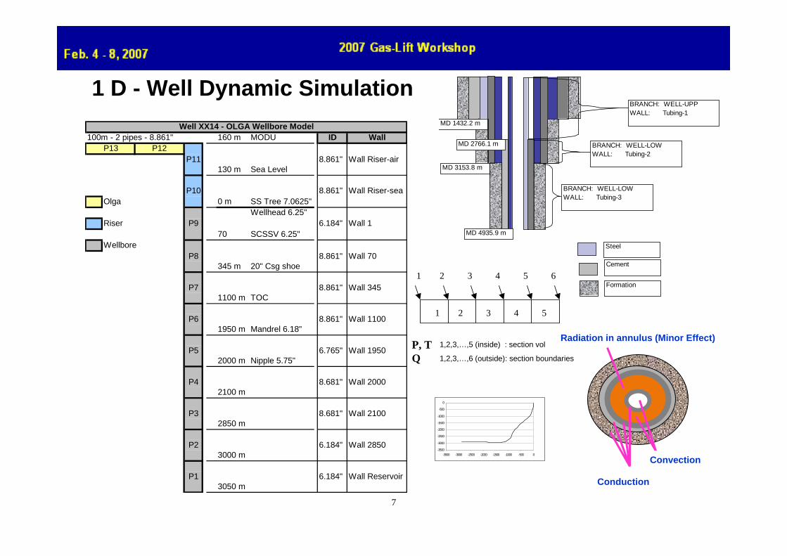
1,2,3,…,5 (inside) : section volumes

1,2,3,…,6 (outside): section boundaries

6

1 D - Well Dynamic Simulation

100m - 2 pipes - 8.861" 160 m MODU ID WallP13 P12

P11 8.861" Wall Riser-air130 m Sea Level

P10 8.861" Wall Riser-seaOlga 0 m SS Tree 7.0625"

Wellhead 6.25"Riser P9 6.184" Wall 1

70 SCSSV 6.25"Wellbore

P8 8.861" Wall 70345 m 20" Csg shoe

P7 8.861" Wall 3451100 m TOC

P6 8.861" Wall 11001950 m Mandrel 6.18"

P5 6.765" Wall 19502000 m Nipple 5.75"

P4 8.681" Wall 20002100 m

P3 8.681" Wall 21002850 m

P2 6.184" Wall 28503000 m

P1 6.184" Wall Reservoir3050 m

Well XX14 - OLGA Wellbore Model

Steel

Cement

Formation

MD 4935.9 m

MD 3153.8 m

BRANCH: WELL-LOWWALL: Tubing-3

MD 2766.1 m BRANCH: WELL-LOWWALL: Tubing-2

MD 1432.2 m

BRANCH: WELL-UPPWALL: Tubing-1

-3500

-3000

-2500

-2000

-1500

-1000

-500

0

-3500 -3000 -2500 -2000 -1500 -1000 -500 0

4

Convection

Conduction

Radiation in annulus (Minor Effect)P, T Q

8

Flow modeling framework

9

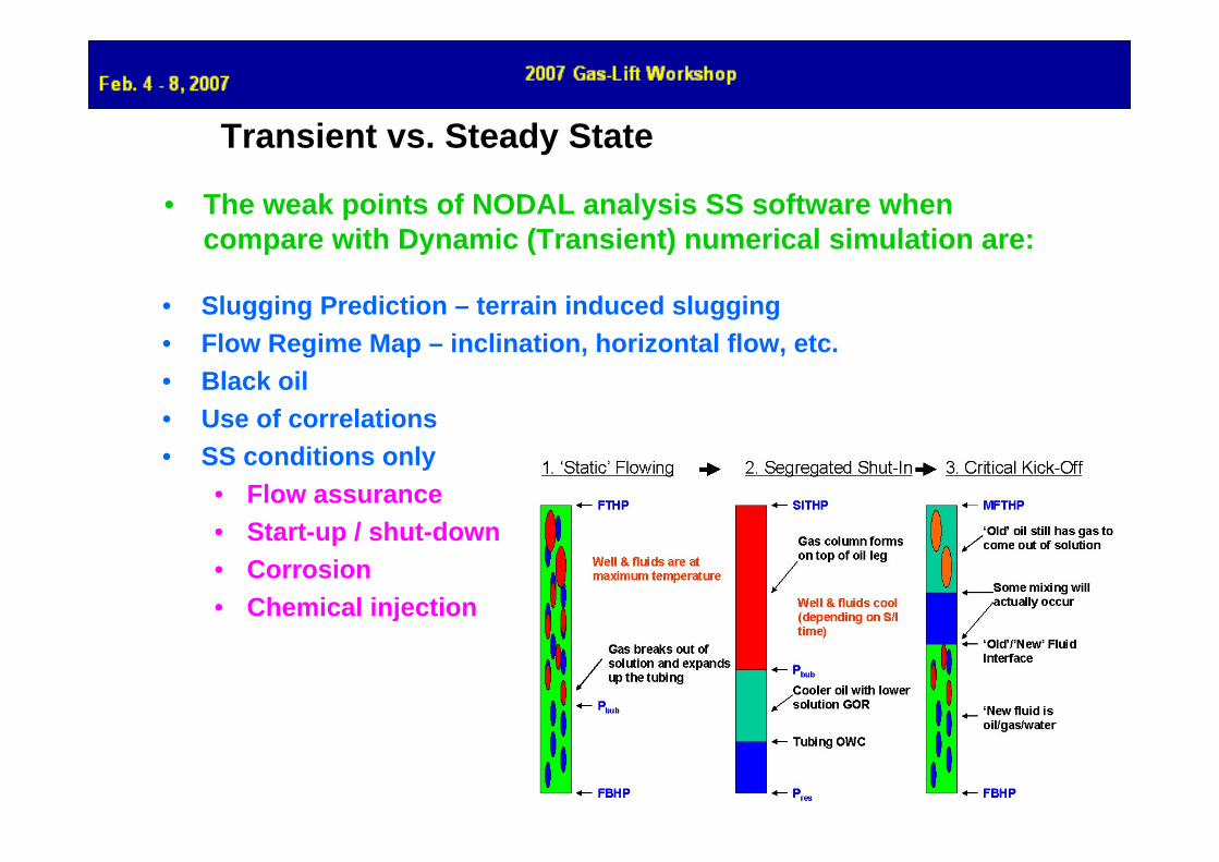
Transient vs. Steady State

• The weak points of NODAL analysis SS software when compare with Dynamic (Transient) numerical simulation are:

• Slugging Prediction – terrain induced slugging• Flow Regime Map – inclination, horizontal flow, etc.• Black oil• Use of correlations• SS conditions only

• Flow assurance• Start-up / shut-down• Corrosion• Chemical injection

10

OLGAS vs Beggs & BrillOLGAS VS Beggs & Brill

7.5" ID 1deg incl

0.00

0.10

0.20

0.30

0.40

0.50

0.60

0.70

0.80

0.00 0.10 0.20 0.30 0.40 0.50 0.60 0.70 0.80

MEASURED LIQUID HOLDUP

PRED

ICTE

D L

IQU

ID H

OLD

UP

OLGASBeggs & Brill

11

Prudhoe Bay 1978 Pressure Drop Data vs. OVIP 1/02 Models, Slug Tracking with DC=182

0

50

100

150

200

250

300

350

400

450

0 50 100 150 200 250 300 350 400 450

Measured Pressure Drop, psi

Pred

icte

d Pr

essu

re D

rop,

psi

Pressure drop prediction for oil pipeline

12

Simulation vs. field data

Northeast Frigg, Liquid Inventory Comparison

0

50

100

150

200

250

300

350

400

450

0.0 1.0 2.0 3.0 4.0 5.0 6.0 7.0Gas Rate, mmSCM/d

Liqu

id In

vent

ory,

m3

Measured

OLGA

13

Why use a transient simulator?

• Normal production– Sizing – diameter, insulation requirement– Stability - Is flow stable? – Gas Lifting / Compressors– Corrosion

• Transient operations– Shut-down and start-up, ramp-up (Liquid and Gas surges)– Depressurisation (tube ruptures, leak sizing, etc.)– Field networks (merging pipelines/well branches with different fluids)

• Thermal-Hydraulics – Rate changes– Shut-in, blow down and start-up / Well loading or unloading– Flow assurance: Wax, Hydrate, Scale, etc.

When things are frozen in time

When not to use dynamic simulation?

Photo: T. Husebø

When things are frozen in time

When not to use dynamic simulation?

Photo: T. Husebø

14

• Pipeline with many dips and humps:– high flow rates: stable flow is possible– low flow rates: instabilities are most likely

(i.e. terrain induced) • Wells with long horizontal sections – Extended Reach• Low Gas Oil Ratio (GOR):

– increased tendency for unstable flow• Gas-condensate lines (high GOR):

– may exhibit very long period transients due to low liquid velocities• Low pressure

– increased tendency for unstable flow • Gas Lift Injection

– Compressors problems, well interference, etc.• Production Chemistry Problems

– Changes in ID caused by deposition• Smart Wells – Control (Opening/Closing valves/sliding sleeves)

Unstable vs. Stable Flow Situations

Multiphase Flow is Transient !Multiphase Flow is Transient !Well Production is Dynamic!Well Production is Dynamic!

15

Usual Potential problems for Stable multiphase flow

• Inclination / Elevation • “Snake” profile• Risers• Rate changes• Condensate – Liquid content in gas• Shut-in / Start up

16

P/T Development – Flow AssuranceTotal System Integration

Oil

Gas Condensate

Pres

sure

Temperature

LIQUID

GAS

GAS + LIQUID

Typical phase envelopes

Gas OilReservoir Temperature

70 -110 oC /160 - 230oF

Emulsion 40oC/104o

F30oC/86oF

20oC/68oF

WaxWater

HydrateHydrate

< 0oC/32oF(Joule Thompson)

~ +4oC/39oF

Temperature effects

OLGA OLGA

OLGA RES ERVOIRS IM U LATOR(ECLIPS E)

OLGA/ D-S PICE

17

OPERATING ENVELOPE

0

100

200

300

400

500

600

700

800

900

1000

0 100 200 300 400 500 600 700 800 900 1000

STANDARD LIQUID RATE [Sm³]

GA

S O

IL R

AT

IO [S

m³/S

m³]

Stable Operating Envelope

Standard Liquid Rate [ Sm³/d]

Gas

Oil

Rat

io [S

m³/

Sm³]

Hydrate Formation Temp. – 18°C

Wax Appearance Temp. – 32°C

Riser Stability – ΔP = 1 bar

Riser Stability – ΔP = 6 bar

Reservoir Pressure – 80 bara Riser Stability – ΔP = 12 bar

Gas Velocity Limit – 12 m/s

Erosional Velocity Limits

18

WELL DYNAMICS • Minimum stable flow rates / Slug Mitigation• Tubing sizing• Flow assurance, Wax , Hydrates / Corrosion rates• Artificial Lift design and optimisation

– Gas Lift Unloading– Compressors shut-down– ESP sizing / Location

• Start-up/Shut-in• Commingling Fluids

– Multiple completions / Multilateral Wells / Smart Wells

• Loading/unloading – Condensate/Water• Well Clean-up• Water accumulation studies• Location of SCSSV• MeOH/Glycol requirements• Well Testing

– Wellbore Storage effects / Segregation effects

19

DYNAMIC GAS LIFT APPLICATIONS

• Well Clean-up using Gas Lift• Well Kick-off using Gas Lift• Gas Lift Unloading• Continuous Gas Lift• Subsea Wellhead Gas Lift• Riser Gas Lift• Single Point (Orifice) Gas Lift

O LG A O LG A

O LG A R ES ER V O IRS IM U L A T O R(EC LIP S E)

O LG A / D -S P IC E

T im e (m in .)

LIQ U ID F L O W IN T O S EP A R A T O R(m / s )3

S LU G F LO W

Fr o n t T a i l F r o n t

S e p a r a t e d f l o w D is p e r se db u b b le

20

Typical Gas Lift Well Configuration

Mud line

Sea level

Injection Gas

Production Fluid

Production Fluid + Injection Gas

Orifice at Injection Point

Unloading Valves

21

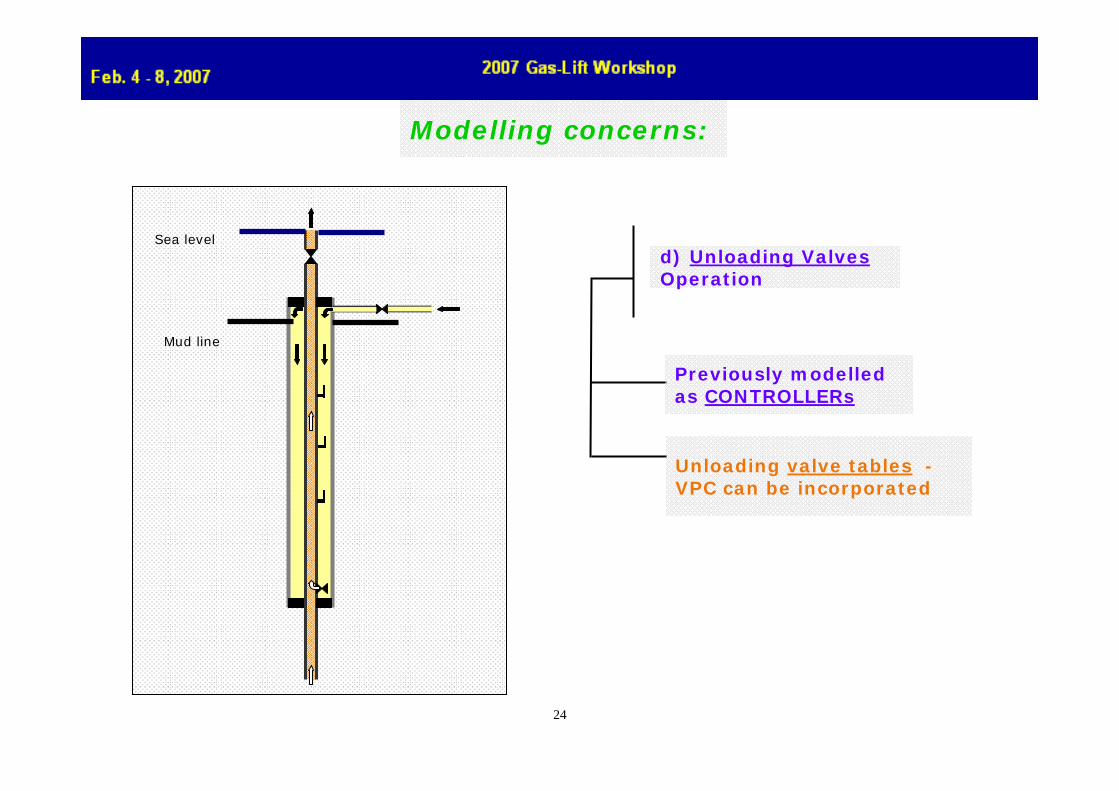
Modelling concerns:

Mud line

Sea level

a) Annular Flow

b) Heat Transfer

c) Non-constant Composition in Tubing above Injection Point

d) Unloading Valves Operation

Typical Gas Lift Well Configuration

Gas Lift is clearly a transient problem

22

Modelling concerns:

a) Annular Flow

b) Heat TransferProduction

Branch = “GASINJ”

Branch = “WELLH”NodeBranch = “WELLB”

Gas Injection

Casing

Full description of annular / tubingflow interactions for flow and heat transfer phenomena

ANNULUS flow model gives very exact counter-current heat exchange

23

c) Non-constant Composition in Tubing above Injection Point

Trend data

Standard OLGACompTrack OLGA

kg/s

40

35

30

25

20

15

10

5

0

Time [h]76.565.554.543.5

Liquid unloading (form of slugging) – Fluid composition varies

Liquid Flowrate at the Wellhead

CompTrack will better account for effects of changing composition in the tubing

Modelling concerns:

24

Mud line

Sea level

Previously modelled as CONTROLLERs

d) Unloading ValvesOperation

Unloading valve tables -VPC can be incorporated

Modelling concerns:

25

Well Unloading Dynamic Simulation

• Following a well workover, tubing and casing are frequently filled with liquid

• Liquid unloaded by injection of gas at casing-head

• Placement and sizing of unloading valves currently performed by approximate steady-state methods

• A transient multiphase simulation can permit more detailed simulation of unloading process

• Troubleshooting can be more efficient using dynamic simulation

26

AC PC

PT

PD

AD

AT

• Valve open when tubing above is full of liquid (liquid weight > opening pressure)

• Valve closes when liquid column weight above location is reduced (< closing pressure)

• Controlled (mostly) by casing pressure

• Valve closure “ripples” down string

• When well unloaded, only orifice at bottom open

Gas Lift Valves (Most Common Configuration)

27

Graphical Steady-State Method

P. Gradient in the Tubingat desired conditions

P. Gradient in the Casing (gas-filled)

P. Gradient of liquid-filledcolumn in the tubing

Safety MarginAPI

28

Gas Lift Valve Performance

Orifice RegionThrottling Region

1 curve per each Casing Injection Pressure

API

29

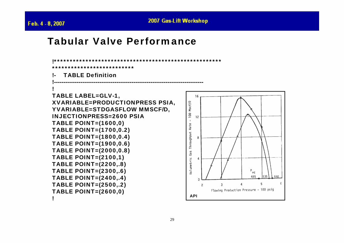
Tabular Valve Performance

!*******************************************************************************!- TABLE Definition!-------------------------------------------------------------------------------!TABLE LABEL=GLV-1, XVARIABLE=PRODUCTIONPRESS PSIA, YVARIABLE=STDGASFLOW MMSCF/D, INJECTIONPRESS=2600 PSIATABLE POINT=(1600,0)TABLE POINT=(1700,0.2)TABLE POINT=(1800,0.4)TABLE POINT=(1900,0.6)TABLE POINT=(2000,0.8)TABLE POINT=(2100,1)TABLE POINT=(2200,.8)TABLE POINT=(2300,.6)TABLE POINT=(2400,.4)TABLE POINT=(2500,.2)TABLE POINT=(2600,0)! API

30

0

1000

2000

3000

4000

5000

6000

0 5 10 15 20 25 30

Time [h]

Oil

rate

[bbl

/d]

0.0

0.5

1.0

1.5

2.0

2.5

Gas

lift

[MM

scfd

]

Gas lift rate Oil rate

Gas Lift – One Injection Point - CGLOil Production

60°F

250°F, 3300 psia and 3 bbl/psi

10000 ft

GOR = 500 scf/bbl

3 1/2”

5 1/2”

500 psia sep press

Choke at injection point

31

Conclusions• Steady-state methods do not capture the transients that inevitably

occur in an operating gas lifted well

• Transient well response occurs during:- Unloading the well - Well shut-down- Normal well operation- Compressor shut-down and injection fluctuations

• Dynamic Simulation can be used to simulate wellbore unloading (gas lift valve tables can be used as input)

• Hydraulics, heat transfer and changes in fluid composition are also taken into account

• Dynamic (flow) Modelling can be an invaluable tool when properly applied (flow assurance, predict fluid properties, etc.) – standard best practice recommendations are required

32

Integrated Modelling ApplicationGas Lift ExampleReservoir-Well-Gas Lift-Flowline-Riser-Separator-Facilities Pigging-405.plt

W1 W2 W3 W4

PCV

LCV

Production Separator

PC

LC

Gas Outlet

Liquid Outlet

Emergency Liquid Outlet

Emergency Drain Valve

ID=2 m, Length=6 mNLL=0.842 mHHLL=1.687LLLL=0.315

Riser

Annulus

Gas LiftID=8-in, Depth=120 m

ID=8-in, Length=4.6 km

Depth=2840 m

Tubing ID=0.1143 m

ID=0.2159 m

• Reservoir: incorporated explicitly

• Facilities: Simple model

33

be dynamic

Thank You! Any Questions?