Co-Investigators:

Parker MacCready, U. Wash.

Andrew Moore, UCSC

Bruce Cornuelle, UCSD

Fei Chai, U. Maine

Federal Partners:

Edward Myers (NOAA NOS CSDL)

Eric Bayler (NOAA JCSDA)

Avichal Mehra (NOAA NWS NCEP)

Igor Shulman (Naval Research Laboratory)

The US West Coast Component of the Coastal Ocean Modeling Testbed

Principal Investigators:

Alexander L. Kurapov, Oregon State University (OSU)

Christopher A. Edwards, University of California at Santa Cruz (UCSC)

Yi Chao, Remote Sensing Solutions, Inc.

Credit : Eric Mortenson, Doug Beghtel /The Oregonian, www.naturalbuy.com, USCG, http://i.livescience.com/, Grantham et al. (2002)

Uses and users of coastal ocean models/products:

Security of US borders / Safe navigation / Search & rescue /Environmental hazard response / Public health / Fisheries management & planning / Recreation / Scientific research

(a)

(b)

(c)

(a) UCSC/CenCCOOS 10-km res. ROMS, 4DVAR (b) RSI/CenCCOOS/SCCOOS 3-km res. ROMS, 3DVAR (c) OSU/NANOOS 2-km res. ROMS, 4DVAR

(d) UW (N. Banas / P. MacCready) .. domain sim. to (c), bio-phys. model

(a)

(b)

(c)

Transition to operations: NOAA West Coast Operational Ocean Forecast System

- Configurations for accurate prediction- Metrics for skill assessment- Data assimilation- Coupled physical bio-chemical OFS

Research questions (Year 3):

Milestones (year 3):

- Complete comparison of the three biochemical models coupled with the regional ocean circulation model

- Transfer tools for WCOFS model setup and evaluation to NOAA NOS CSDL - Provide recommendations to NOAA about the choice of the assimilation method

for WCOFS for based on comparison 4DVAR and hybrid methods, 3DVAR and EnKF

- Does the ensemble-variational hybrid approach to data assimilation improve accuracy of state estimates and forecasts in dynamic coastal ocean regions, compared to a more traditional approach (a variational method with a static initial condition covariance)?

- Can observation impact and observation sensitivity experiments reveal elements of the west coast observation network that provide particularly critical or quantitatively redundant data for state estimation as gauged by particular metrics?

- Does added ecosystem model complexity provide benefits for modeling the CCS ecosystem?

OR-WA model: traditional 4DVAR vs. ensemble-variational approach

(Kurapov and Pasmans)

4DVAR: dynamically-based smoothing over a larger time interval

Pros:- Transients are left in the past- Data error is filtered in time- Time-average data may be assimilated

Challenges:- Requires development and repeated implementation of the adjoint model

component- The IC error covariance is static (the same in each analysis interval)

timeAnalysis interval(correcting IC)

f

a

f

a f

Hybrid Ensemble - 4DVAR (Kurapov and Pasmans)

time

f

a

f

af

Obtain the IC error covariance from an ensemble of forecasts

Challenges: - Ensemble generation - Covariance localization (Pasmans & Kurapov, 2016, in prep.)

Analysis interval(correcting IC)

(incorporate in EnKF – DART ? .. Cornuelle et al.)

The ens-var method shows DA limitations predicting unassimilated fields, such as salinity in the far reach of the Columbia R. plume

SSS on 05/13/2011 before assimilation

(DA: GOES SST, HF radar uv and altimetry are assimilated)

SSS on 05/13/2011 before assimilation after assimilation

A negative 4DVAR correction (color)(contours show SSS) 05/04/2011

Negative correction in SST => (given strong negative covar. of T and S in the plume) positive SSS correction

Update on WCOFS

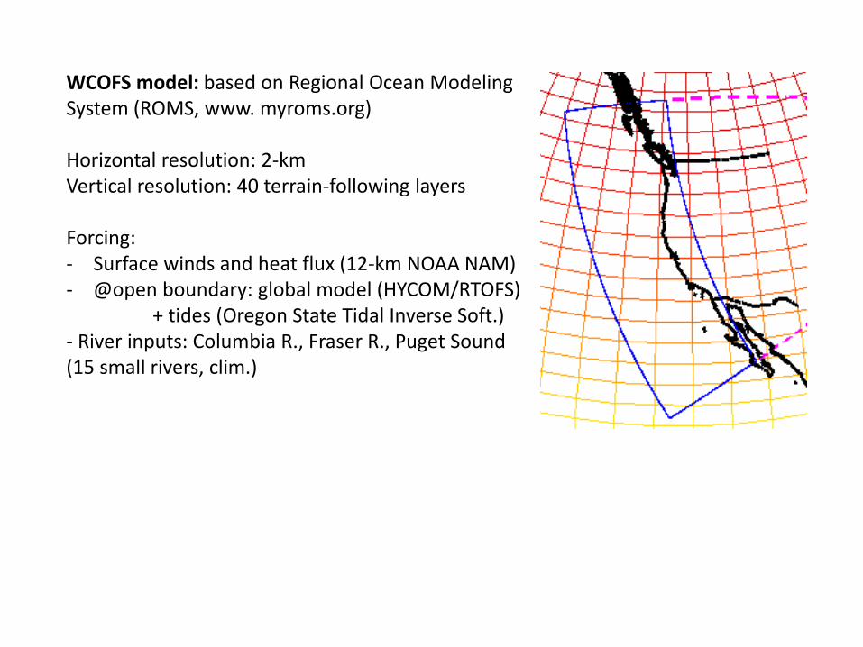
WCOFS model: based on Regional Ocean Modeling System (ROMS, www. myroms.org)

Horizontal resolution: 2-kmVertical resolution: 40 terrain-following layers

Forcing: - Surface winds and heat flux (12-km NOAA NAM)- @open boundary: global model (HYCOM/RTOFS)

+ tides (Oregon State Tidal Inverse Soft.) - River inputs: Columbia R., Fraser R., Puget Sound (15 small rivers, clim.)

WCOFS: present status / skill assessment / initial data assimilation steps

Model-data comparisons:- Coastal sea level (against tide gauge data)- Alongshore coastal currents (against HF radar)- SST (against moored time series, satellite)- Subsurface stratification (Argo floats, gliders)

Scientific analyses (using a 6-year, 2009-2014, simulation without assimilation)- Alongshore SSH coherence maps / esp. long-period motions- Warm anomaly in the NEP in 2014-2015- Seasonal and interannual variability in the slope properties (esp. undercurrent)

Initial DA efforts: - learn to use the ROMS 4DVAR machine, first in a small domain

Along-coast coherence in the coastal sea level (tide gauge vs. model): close in amplitude and phase

Coherence = spatial correlation for a specified frequency range

Shown here for the range of periods close to 10 days

w/ resp. to San Diego, CA w/ resp to Newport, OR

amplitude

phase (along-shore propagation)

Using the 6-year model solution, we can compute 2-dimenstional SSH coherence amplitude maps and learn about spatial structure of the long coastal trapped waves (conduits of the signal from south to north)

Frequency range centered on =1/5 d-1

Kurapov et al., Oc. Dyn., submitted

Frequency range centered on =1/10 d-1

Reference point

wave scattering and dissipation over complicated topography south of Santa Barbara Channel

The SSH coherence amplitude map

Frequency range centered on =1/60 d-1

(40-126 days)

The SSH coherence amplitude map

Reference point

Longer period coastal ocean signal propagates through the Santa Barbara Channel

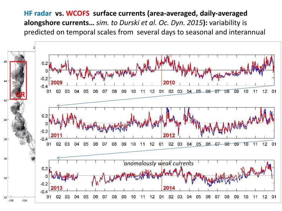
HF radar vs. WCOFS surface currents (area-averaged, daily-averaged alongshore currents… sim. to Durski et al. Oc. Dyn. 2015): variability is predicted on temporal scales from several days to seasonal and interannual

OR

anomalously weak currents

Near-surface T (NDBC shelf moorings) / WCOFS comparison:

off Newport, OR

off La Jolla, CA

WCOFS has predicted correctly the warming trend (Dec 2013 – Dec 2014)

Compared to sat. SST anomaly, WCOFS predicts the appearance of the warm blob by Jan 2014, and wide-spread warming along the US Coast by summer 2014

Satellite SSTA (OSTIA)

Model SSTA (WCOFS)

Anomaly w/ respect to 2009-2013 climatology (computed similarly for sat. and model)

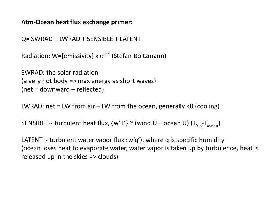
Atm-Ocean heat flux exchange primer:

Q= SWRAD + LWRAD + SENSIBLE + LATENT

Radiation: W=[emissivity] x T4 (Stefan-Boltzmann)

SWRAD: the solar radiation (a very hot body => max energy as short waves) (net = downward – reflected)

LWRAD: net = LW from air – LW from the ocean, generally <0 (cooling)

SENSIBLE turbulent heat flux, w’T’ ~ (wind U – ocean U) (TAIR-Tocean)

LATENT turbulent water vapor flux w’q’, where q is specific humidity (ocean loses heat to evaporate water, water vapor is taken up by turbulence, heat is released up in the skies => clouds)

ROMS SWRAD anomaly 2013 w resp to 2009-2013 clim (using 3-mo running ave)

Winter 2013-14: SWRAD not anomalously large

ROMS SWRAD anomaly 2014 w respect to 2009-2013 clim (using 3-mo running ave)

Anomalously large SWRAD in summer 2014

Latent, 2013 anomaly

Non-negligible (>40W/m2) negative anomaly in late summer

Latent, 2014 anomaly

Implication for WCOFS: presently, atm-oce salin. flux = 0. Cooling by latent heat flux is associated with evaporation (positive salinity flux). Can this cause convective mixing that will help to cool the surface b. layer?

Analyses on the =26.5 isopycnalsurface

6-year averaged properties along the meridional section

between 26.5 and 26.25

Dots: Argo floats

If we provide enough resolution, we start to see eddy generation and material exchange between slope and interior ocean

Shown is a snapshot of temperature on =26.5. 1 June 2012 / 2013 / 2014.

Analyses of slope properties on the isopycnalsurface =26.5 kg/m3

In the entire domain, for each day, at each grid point we obtain

- depth of the isopycnal surface, z(x,y,t)- T, S, u, v on this surface

Average properties in cross-shore direction offshore of the 200-m isobath (30-km wide)

e.g., z(s,t), T(s,t) where s = distance from southern boundary

T(s,t)= time_ave_T(s) + seasonal_T(s,t)+anomaly_T(s,t)

seasonal_T = harmonic fit (annual + semi-annual)

Effect of CTW? Effect of undercurrent?Climatology, anomalies?

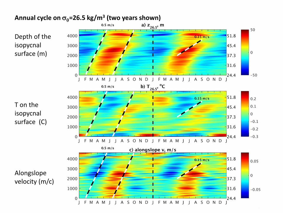
Annual cycle on =26.5 kg/m3 (two years shown)

Depth of the isopycnalsurface (m)

T on the isopycnalsurface (C)

Alongslopevelocity (m/c)

Initial assimilation tests: use JPSS VIIRS L3U, in the Central CA subdomain

(a) Over a given time interval (here, 3 days) use available observations and adjoint model to correct initial conditions for the forecast

-3d -2d -1d 0

(b) Run the model forecast using improved initial conditions

1 Jun 2 Jun 3 Jun

Example of SST coverage: JPSS L3U, in central CA, Jun 1-3 2014 (data: courtesy A. Ignatov)

DA: a dynamically based time-space interpolator (fills between gaps, facilitates accurate forecasts)

Assimilation methodology, 4DVAR:

The effect of SST assimilation on model SST:

06/02/16, 00:00:00 UTC

Model before assimilation / after assimilation

Tracks from 3 satellites (Jason2, Cryosat2, Altika) – 1-3 June 2014

SSH anomaly along the satellite track inside the CCA4 domain model SSH forecast along the same track

SSH depression: evidence of a cyclonic eddy

jun-1-2016

Next step: tests assimilating SST in combination with alongtrack altimetry

Data: RADS SSH (NESDIS/STAR, L. Miller et al.)

What does altimetry provide?- the non-tidal sea surface slope on horizontal scales 50 km and larger provides information on the “geostrophic” currents (characteristic of eddies, coastal currents) in the direction across the satellite pass.

Year 4 plans:

• Forecasts provided by our model systems will be compared to available in-situ and satellite observations (Kurapov, Edwards, Chao, MacCready)

• Carbon variables (Alkalinity and DIC) will be added to the 6-component NPZDO-Banas model, and compared with observations (MacCready)

• The OR-WA 4DVAR system will be tested with a new (ensemble-based) model error covariance suitable for anisotropic ocean conditions in the presence of the Columbia River (Kurapov)

• The impact of glider and mooring data on coastal ocean prediction will be tested (Kurapov, Chao)

• The data assimilation methods (e.g., 3DVAR, 4DVAR and ensemble Kalman Filter) will be compared and evaluated (Chao, Cornuelle, Moore)

• Observing system simulation experiments (OSSE) will be performed for the regional UCSC model using observation sensitivity and observation impact tools developed for ROMS (Moore)

• In conjunction with NOAA CSDL, key metrics for physical forecast evaluation and will be tested (all participants)

• Metrics for skill assessment of biogeochemical fields, including Hypoxia and OA, will be developed (Edwards, Chai, MacCready)

• Available solutions will be contributed to COMT CI (all participants)

Transition to NOAA operations:

• One or more biogeochemical components will be tested in the WCOFS configuration (all participants, year 4-5)

• Feasibility of using ROMS 4DVAR in WCOFS will be tested (Moore, Kurapov)