The U.S. Current Account and the Dollar

Olivier Blanchard Francesco Giavazzi Filipa Sa ∗

March 21, 2005

Abstract

There are two main forces behind the large U.S. current account deficits.First, an increase in the U.S. demand for foreign goods. Second, an increasein the foreign demand for U.S. assets.

Both forces have contributed to steadily increasing current account deficitssince the mid–1990s. This increase has been accompanied by a real dollarappreciation until late 2001, and a real depreciation since. The depreciationaccelerated in late 2004, raising the questions of whether and how muchmore is to come, and if so, against which currencies, the euro, the yen, orthe renminbi.

Our purpose in this paper is to explore these issues. Our theoretical contri-bution is to develop a simple model of exchange rate and current accountdetermination based on imperfect substitutability in both goods and as-set markets, and to use it to interpret the past and explore alternativescenarios for the future. Our practical conclusions are that substantiallymore depreciation is to come, surely against the yen and the renminbi, andprobably against the euro.

∗ MIT and NBER, MIT, NBER, CEPR and Bocconi, and MIT respectively. Preparedfor the BPEA meetings, April 2005. An earlier version, with the same title, was circulatedas MIT WP 05-02, January 2005. We thank Ricardo Caballero, Menzie Chinn, GuyDebelle, Ken Froot, Pierre Olivier Gourinchas, Maury Obstfeld, Helene Rey, Ken Rogoff,Nouriel Roubini for comments. We also thank Nigel Gault, Brian Sack, Catherine Mann,Gian Maria Milesi-Ferretti and Philip Lane for help with data.

1

There are two main forces behind the large U.S. current account deficits:

First, an increase in the U.S. demand for foreign goods, partly because ofrelatively higher U.S. growth, partly because of shifts in demand away fromU.S. goods towards foreign goods.

Second, an increase in the foreign demand for U.S. assets, starting withhigh foreign private demand for U.S. equities in the second half of the1990s, shifting to foreign private and then central bank demands for U.S.bonds in the 2000s.

Both forces have contributed to steadily increasing current account deficitssince the mid–1990s. This increase has been accompanied by a real dollarappreciation until late 2001, and a real depreciation since. The depreciationaccelerated in late 2004, raising the issues of whether and how much moreis to come, and if so, against which currencies, the euro, the yen, or therenminbi.

These are the issues we take up in this paper. We do so by developinga simple model of exchange rate and current account determination, andusing it to interpret the past and explore the future.

We start by developing the model. Its central assumption is of imperfectsubstitutability not only between U.S. and foreign goods, but also betweenU.S. and foreign assets. This allows us to discuss not only the effects of shiftsin the relative demand for goods, but also of shifts in the relative demandfor assets. We show that increases in U.S. demand for foreign goods lead toan initial depreciation, followed by further depreciation over time. Increasesin foreign demand for U.S. assets lead instead to an initial appreciation,followed by depreciation over time, to a level lower than before the shift.

The model provides a natural interpretation of the past. Increases in U.S.demand for foreign goods and increases in foreign demand for U.S. assetshave combined to increase the current account deficit. While the initial neteffect of the two shifts was to lead to a dollar appreciation, they both imply

2

an eventual depreciation. The United States appears to have entered thisdepreciation phase.

The model also provides a way of examining the future. How much depre-ciation is to come, and at what rate, depends on where we are, and on thefuture evolution of shifts in the demand for goods and the demand for as-sets. This raises two main issues. Can we expect the trade deficit to largelyreverse itself—at a given exchange rate? If it does, the needed deprecia-tion will obviously be smaller. Can we expect the foreign demand for U.S.assets to continue to increase? If it does, the depreciation will be delayed—although it will still have to come eventually. While there is substantialuncertainty about the answers, we conclude that neither scenario is likely.This leads us to anticipate, absent surprises, more dollar depreciation tocome, at a small but steady rate.

Surprises will however take place; only their sign is unknown... We againuse the model as a guide to discuss a number of alternative scenarios, fromthe abandonment of the peg of the renminbi to changes in the compositionof reserves by Asian Central Banks, to changes in U.S. interest rates.

This leads us to the last part of the paper, where we ask how much ofthe depreciation is likely to take place against the Euro, how much againstAsian currencies. We extend our model to allow for more than two coun-tries. We conclude that, absent surprises, the path of adjustment is likelyto be associated primarily with an appreciation of Asian currencies, butalso with a further appreciation of the euro vis a vis the dollar.

1 A Model of the Exchange Rate and the Current

Account

Much of the economists’ intuition about joint movements in the exchangerate and the current account is based on the assumption of perfect substi-

3

tutability between domestic and foreign assets. As we shall show, introduc-ing imperfect substitutability substantially changes the scene. Obviously, itallows us to think about the dynamic effects of shifts in asset preferences.But it also modifies the dynamic effects of shifts in preferences with respectto goods.

A note on the relation of our model to the literature: We are not the firstto insist on the potential importance of imperfect substitutability. Indeedthe model we present below builds on two old (largely and unjustly forgot-ten) papers, by Henderson and Rogoff [1982], and, especially, Kouri [1983].1

Both papers relax the interest parity condition and assume instead imper-fect substitutability of domestic and foreign assets. Henderson and Rogofffocus mainly on issues of stability. Kouri focuses on the effects of changesin portfolio preferences and the implications of imperfect substitutabilitybetween assets for shocks to the current account.

Our value added is in allowing for a richer description of gross asset posi-tions. By doing this, we are able to incorporate in the analysis the “val-uation effects” which have been at the center of recent empirical researchon gross financial flows—in particular by Gourinchas and Rey [2004] andLane and Milesi–Ferretti [2002], [2004]—, and play an important role in thecontext of U.S. current account deficits. Many of the themes we develop,from the role of imperfect substitutability and valuation effects, have alsobeen recently emphasized by Obstfeld [2004].

1. The working paper version of the paper by Kouri dates from 1976. One could arguethat there were two fundamental papers written that year on this issue, one by Dornbusch[1976], who explored the implications of perfect substitutability, the other by Kouri, whoexplored the implications of imperfect substitutability. The Dornbusch approach, and itspowerful implications, has dominated research since then. But imperfect substitutabilityseems central to the issues we face today.

4

The Case of Perfect Substitutability

To see how imperfect substitutability of assets matters, it is best to startfrom the well understood case of perfect substitutability.

Think of two countries, domestic (say the United States) and foreign (therest of the world). We can think of the current account and the exchangerate as being determined by two relations.

The first is the uncovered interest parity condition:

(1 + r) = (1 + r∗)E

Ee+1

where r and r∗ are U.S. and foreign real interest rates respectively (starsdenote foreign variables), E is the real exchange rate, defined as the relativeprice of U.S. goods in terms of foreign goods (so an appreciation is anincrease in the exchange rate), and Ee

+1 is the expected real exchange ratenext period. The condition states that expected returns on US and foreignassets must be equal.

The second is the equation giving net debt accumulation:

F+1 = (1 + r)F + D(E+1, z+1)

D(E, z) is the trade deficit. It is an increasing function of the real exchangerate (so DE > 0). All other factors—changes in U.S. or foreign levels ofspending, or shifts in U.S. or foreign relative demands at a given exchangerate and given activity levels—are captured by the shift variable z. Byconvention, an increase in z is assumed to worsen the trade balance, soDz > 0. F is the net debt of the United States, denominated in terms ofU.S. goods. The condition states that net debt next period is equal to netdebt this period times one plus the interest rate, plus the trade deficit nextperiod.

5

Assume that the trade deficit is linear in E and z, so D(E, z) = θE + z.Assume also, for convenience, that U.S. and foreign interest rates are equal,so r∗ = r, and constant. From the interest parity condition, it follows thatthe expected exchange rate is constant and equal to the current exchangerate. The value of the exchange rate is obtained in turn by solving out thenet debt accumulation forward and imposing the condition that net debtdoes not explode faster than the interest rate. Doing this gives:

E = −r

θ[F−1 +

11 + r

∞∑

0

(1 + r)−i ze+i ]

The exchange rate depends negatively on the initial net debt position andon the sequence of current and expected shifts to the trade balance.

Replacing the exchange rate in the net debt accumulation equation givesin turn:

F+1 − F = [z − r

1 + r

∞∑

0

(1 + r)−i ze+i ]

The change in the net debt position depends on the difference between thecurrent shift and the present value of future shifts to the trade balance.

For our purposes, these two equations have one main implication. Consideran unexpected, permanent, increase in z at time t by ∆z—say an increasein the U.S. demand for Chinese goods (at a given exchange rate). Then,from the two equations above:

E − E−1 = −∆z

θ; F+1 − F = 0

In words: Permanent shifts lead to a depreciation large enough to maintaincurrent account balance. By a similar argument, shifts that are expectedto be long lasting lead to a large depreciation, and only a small currentaccount deficit. As we shall argue later, this is not what has happenedin the United States over the last 10 years. The shift in z appears to be,

6

if not permanent, at least long lasting. Yet, it has not been offset by alarge depreciation, but has been reflected instead in a large current ac-count deficit. This we shall argue, is the result of two factors, both closelylinked to imperfect substitutability. The first is that, under imperfect sub-stitutability, the initial depreciation in response to increases in z is morelimited, leading initially to a current account deficit. The second is that,under imperfect substitutability, there can be shocks to asset preferences.These shocks lead to an initial appreciation and a current account deficit.And they have indeed played an important role since the mid 1990s.

Imperfect Substitutability and Portfolio Balance

We now introduce imperfect substitutability between assets. Let W denotethe wealth of U.S. investors, measured in units of U.S. goods. W is equalto the stock of U.S. assets, X, minus the net debt position of the UnitedStates, F :

W = X − F

Similarly, let W ∗ denote foreign wealth, and X∗ foreign assets, both interms of foreign goods. Then, the wealth of foreign investors, expressed interms of U.S. goods, is given by:

W ∗

E=

X∗

E+ F

Let R be the relative expected gross real rate of return on holding U.S.assets versus foreign assets:

R ≡ 1 + r

1 + r∗Ee

+1

E(1)

U.S. investors allocate their wealth W between U.S. and foreign assets.They allocate a share α to U.S. assets, and by implication a share (1− α)to foreign assets. Symmetrically, foreign investors invest a share α∗ of their

7

wealth W ∗ in foreign assets, and a share (1 − α∗) in U.S. assets. Assumethat these shares are functions of the relative rate of return, so

α = α(R, s), αR > 0, αs > 0 α∗ = α∗(R, s), α∗R < 0 α∗s < 0

A higher rate of return on U.S. assets increases the U.S. share in U.S. assets,and decreases the foreign share in foreign assets. s is a shift factor, standingfor all the factors which shift portfolio shares for a given relative return.By convention, an increase in s leads both U.S. and foreign investors toincrease the share of their portfolio in U.S. assets for a given relative rateof return.

An important parameter in the model is the degree of home bias in U.S. andforeign portfolios. We assume that there is indeed home bias, and capture itby assuming that the sum of portfolio shares falling on own-country assetsexceeds one:

α(R, s) + α∗(R, s) > 1

Equilibrium in the market for U.S. assets (and by implication, in the marketfor foreign assets) implies

X = α(R, s) W + (1− α∗(R, s))W ∗

E

The supply of U.S. assets must be equal to U.S. demand plus foreign de-mand. Given the definition of F introduced earlier, this condition can berewritten as

X = α(R, s)(X − F ) + (1− α∗(R, s)) (X∗

E+ F ) (2)

where R is given in turn by equation (1), and depends in particular on E

and Ee+1.

8

This gives us the first relation, which we shall refer to as the portfolio

balance relation, between net debt, F , and the exchange rate, E. Theslope of the relation between net debt and the exchange rate, evaluated atr = r∗ and Ee

+1 = E so R = 1, is given by

dE/E

dF= −α(1, s) + α∗(1, s)− 1

(1− α∗(1, s))X∗/E< 0

So, in the presence of home bias, higher net debt is associated with a lowerexchange rate. The reason is that, as wealth is transfered from the UnitedStates to the rest of the world, home bias leads to a decrease in the demandfor U.S. assets, which in turn requires a decrease in the exchange rate.

Imperfect Substitutability and Current Account Balance

Assume, as before, that U.S. and foreign goods are imperfect substitutes,and the U.S. trade deficit, in terms of U.S. goods, is given by:

D = D(E, z), DE > 0, Dz > 0

Turn now to the equation giving the dynamics of the U.S. net debt position.Given our assumptions, U.S. net debt is given by:

F+1 = (1−α∗(R, s))W ∗

E(1+r) − (1−α(R, s)) W (1+r∗)

E

E+1+ D(E+1, z+1)

Net debt next period is equal to the value of U.S. assets held by foreign in-vestors next period, minus the value of foreign assets held by U.S. investorsnext period, plus the trade deficit next period:

• The value of U.S. assets held by foreign investors next period isequal to their wealth in terms of U.S. goods this period, times the

9

share they invest in U.S. assets this period, times the gross rate ofreturn on U.S. assets in terms of U.S. goods.

• The value of foreign assets held by U.S. investors next period isequal to U.S. wealth this period, times the share they invest inforeign assets this period, times the realized gross rate of return onforeign assets in terms of U.S. goods.

The previous equation can be rewritten as

F+1 = (1+r)F +(1−α(R, z))(1+r)(1− 1 + r∗

1 + r

E

E+1)(X−F )+D(E+1, z+1)

(3)We shall call this the current account balance relation.

The first and last terms on the right are standard: Next period net debt isequal to this period net debt times the gross rate of return, plus the tradedeficit next period.

The term in the middle reflects valuation effects, recently stressed by Gour-inchas and Rey [2004], and Lane and Milesi–Ferretti [2004].2 Consider forexample an unexpected decrease in the price of U.S. goods, an unexpecteddecrease in Ee

+1 relative to E—a dollar depreciation for short.

This depreciation increases the dollar value of U.S. holdings of foreign as-sets, decreasing the net debt U.S. position. Put another way, a deprecia-tion improves the U.S. net debt position in two ways, the conventional onethrough the improvement in the trade balance, the second through asset

2. So long as the net debt position is the result of partly offsetting gross positions,valuation effects are present whether or not domestic and foreign assets are perfectsubstitutes. (Following standard practice, we ignored them in the model presented earlierby implicitly assuming that, if net debt was positive, U.S. investors did not hold foreignassets and net debt was therefore equal to the foreign holdings of U.S. assets.) Underperfect substitutability however, there is no guide as to what determines the alphas, andtherefore what determines the gross positions of U.S. and foreign investors.

10

revaluation. Note that:

• The strength of the valuation effects depends on gross rather thannet positions, and so on the share of the U.S. portfolio in foreignassets, (1− α), and on the size of U.S. wealth, X − F . It is presenteven if F = 0.

• The strength of valuation effects depends on our assumption thatU.S. gross liabilities are denoted in dollars, and so their value in dol-lars are unaffected by a dollar depreciation. Valuation effects wouldobviously be very different when, as is typically the case for emergingcountries, gross positions were smaller, and liabilities were denomi-nated in foreign currency.

Steady State and Dynamics

Assume the stocks of assets X, X∗, and the shift variables z and s, to beconstant. Assume also r and r∗ to be constant and equal to each other. Inthis case, the steady state values of net debt F and E are characterized bytwo relations:

The first is the portfolio balance equation (2). Given the equality of interestrates and the constant exchange rate, R = 1 and the relation takes the form:

X = α(1, s)(X − F ) + (1− α∗(1, s)) (X∗

E+ F )

The second is the current account balance equation (3). Given the equalityof interest rates and the constant exchange rate and net debt levels, therelation takes the form:

0 = rF + D(E, z)

The first relation implies a negative relation between net debt and theexchange rate: As we saw earlier, in the presence of home bias, higher U.S.net debt, which transfers wealth to foreign investors, shifts demand away

11

from U.S. assets, and thus lowers the exchange rate.

The second relation also implies a negative relation between net debt andthe exchange rate. The higher the net debt, the higher the trade surplusrequired in steady state to finance interest payments on the debt, thus thelower the exchange rate.3

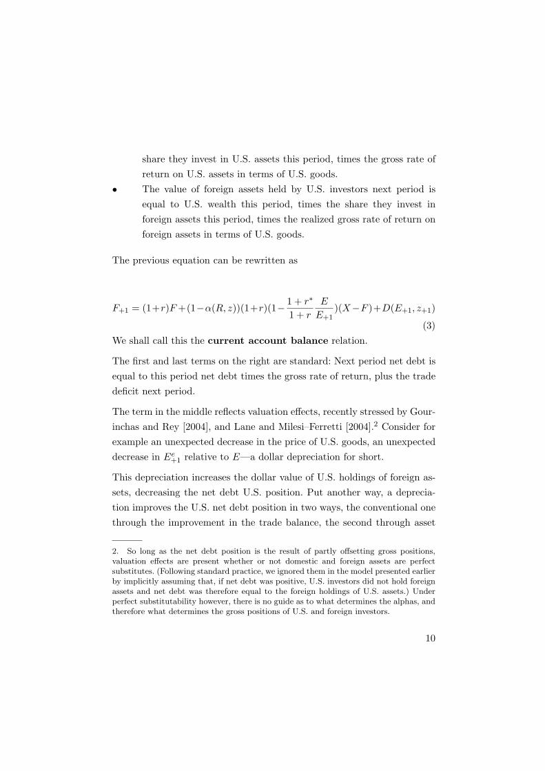
This raises the question of the stability of the system. The system is (locallysaddle point) stable if, as drawn in Figure 1, the portfolio balance relationis steeper than the current account balance equation.4 To understand thiscondition, consider an increase in U.S. net debt. This increase has twoeffects on the current account deficit, and thus on the change in net debt:It increases interest payments. It leads, through portfolio balance, to a lowerexchange rate, and thus a decrease in the trade deficit. For stability, thenet effect must be that the increase in net debt reduces the current accountdeficit. This condition appears to be satisfied for plausible parameter values(more in the next section), and we shall assume that it is satisfied here. Inthat case, the path of adjustment—the saddle path—is downward sloping,as drawn in Figure 1.

We can now characterize the effects of shifts in preferences for goods or forassets.

The Effects of a Shift Towards Foreign Goods

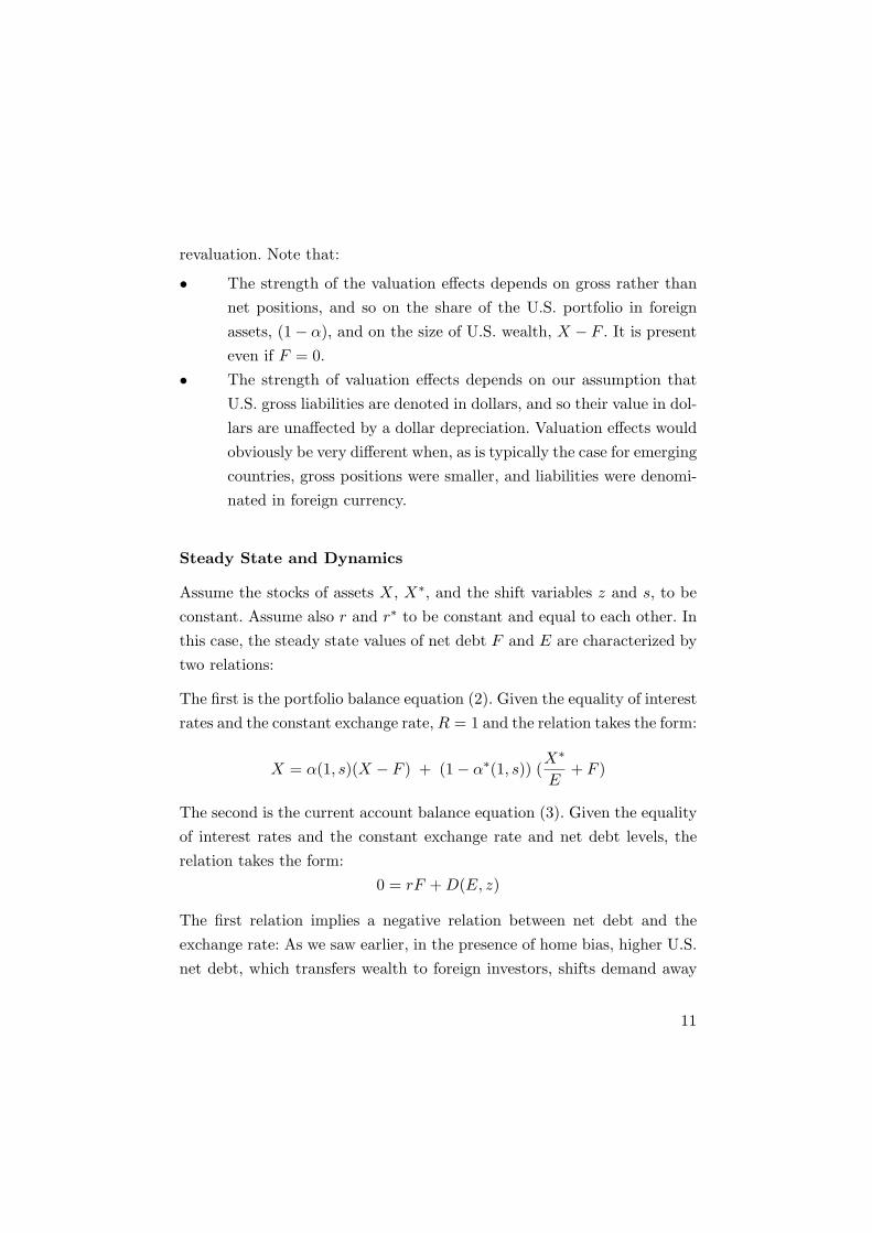
Figure 2a shows the effect of an (unexpected and permanent) increase in z.One can think of z as coming either from increases in U.S. activity relativeto foreign activity, or from a shift in exports or imports at a given level of

3. If we had allowed r and r∗ to differ, the relation would have an additional termand take the form: 0 = rF + (1 − α(R))(r − r∗)(X − F ) + D(E, z). This additionalterm implies that if, for example, a country pays a lower rate of return on its liabilitiesthan it receives on its assets, it may be able to combine positive net debt with positivenet income payments from abroad—the situation the United States was in until veryrecently.4. A characterization of the dynamics is given in the appendix.

12

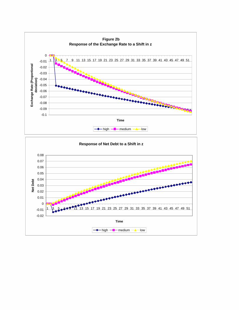
Figure 2b Response of the Exchange Rate to a Shift in z

-0.1

-0.09

-0.08

-0.07

-0.06

-0.05

-0.04

-0.03

-0.02

-0.01

01 3 5 7 9 11 13 15 17 19 21 23 25 27 29 31 33 35 37 39 41 43 45 47 49 51

Time

Exch

ange

Rat

e (P

ropo

rtio

nal

devi

atio

n)

high medium low

Response of Net Debt to a Shift in z

-0.02

-0.01

0

0.01

0.02

0.03

0.04

0.05

0.06

0.07

0.08

1 3 5 7 9 11 13 15 17 19 21 23 25 27 29 31 33 35 37 39 41 43 45 47 49 51

Time

Net

Deb

t

high medium low

activity and a given exchange rate; we defer a discussion of the sources ofthe actual shift in z over the past decade in the United States to later.

For a given level of net debt, current account balance requires a lowerexchange rate: The current account balance locus shifts down. The newsteady state is at point C, associated with a lower exchange rate and ahigher level of net debt.

Valuation effects imply that any unexpected depreciation leads to an unex-pected decrease in the net debt position. Denoting by ∆E the unexpectedchange in the exchange rate at the time of the shift, it follows from equa-tion (3) that the relation between the two at the time of the shift is givenby:

∆F = (1− α)(1 + r∗)(X − F )∆E

E(4)

The economy jumps initially from A to B, and then converges over timealong the saddle point path, from B to C. The shift in the trade deficit leadsto an initial, unexpected, depreciation, followed by further depreciation andnet debt accumulation over time until the new steady state is reached.

Note that the degree of substitutability between assets does not affectthe steady state (more formally: note that the steady state depends onα(1, s) and α∗(1, s), so changes in αR and α∗R which leave α(1, s) andα∗(1, s) unchanged do not affect the steady state.) In other words, theeventual depreciation is the same no matter how close substitutes U.S. andforeign assets are. But the degree of substitutability plays a central rolein the dynamics of adjustment, and in the respective roles of the initialunexpected depreciation and the anticipated depreciation thereafter. Thisis shown in Figure 2b, which shows the effects of three different values ofαR and α∗R, on the path of adjustment (The three simulations are basedon values for the parameters discussed and introduced in the next section.The purpose here is just to show qualitative properties of the paths. Weshall return to the quantitative implications later.)

13

The less substitutable U.S. and foreign assets are—the smaller αR andα∗R—the smaller the initial depreciation, and the larger the anticipatedrate of depreciation thereafter. To understand why, consider the extremecase where the shares do not depend on rates of return: U.S. and foreigninvestors want to maintain constant shares, no matter what the relativerate of return is. In this case, the portfolio balance equation (2) impliesthat there will be no response of the exchange rate to the unexpectedchange in z at the time it happens: Any movement in the exchange ratewould be inconsistent with equilibrium in the market for U.S. assets. Only,over time, as the deficit leads to an increase in net debt, will the exchangerate decline.

Conversely, the more substitutable U.S. and foreign assets are, the largerwill be the initial depreciation, and the smaller the anticipated rate ofdepreciation thereafter, the longer the time to reach the new steady state.The limit of perfect substitutability—corresponding to the model we sawat the start—is actually degenerate: The initial depreciation is such as tomaintain current account balance, and the economy does not move fromthere on, never reaching the new steady state (and so, the anticipated rateof depreciation is equal to zero.)

To summarize, in contrast to the case of perfect substitutability betweenassets we saw earlier, an increase in the U.S. demand for foreign goodsleads to a limited depreciation initially, a potentially large and long lastingcurrent account deficit, and a steady depreciation over time.

The Effects of a Shift Towards U.S. Assets

Figure 3a shows the effect of an (unexpected and permanent) increase ins, an increase in the demand for U.S. assets. Again, we defer a discussionof the potential factors behind such an increase in demand to later.

By assumption, the increase in s leads to an increase in α(1, s) and a

14

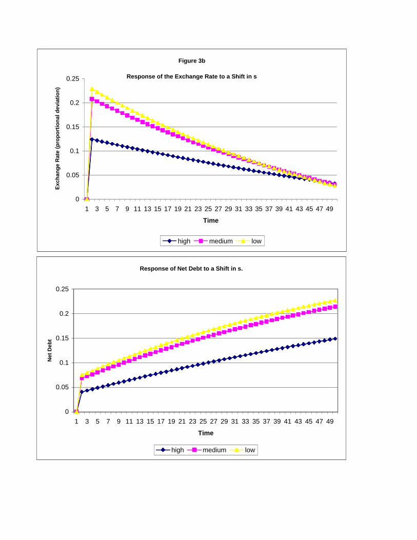
Figure 3b

Response of the Exchange Rate to a Shift in s

0

0.05

0.1

0.15

0.2

0.25

1 3 5 7 9 11 13 15 17 19 21 23 25 27 29 31 33 35 37 39 41 43 45 47 49

Time

Exch

ange

Rat

e (p

ropo

rtio

nal d

evia

tion)

high medium low

Response of Net Debt to a Shift in s.

0

0.05

0.1

0.15

0.2

0.25

1 3 5 7 9 11 13 15 17 19 21 23 25 27 29 31 33 35 37 39 41 43 45 47 49

Time

Net

Deb

t

high medium low

decrease in α∗(1, s). At a given level of net debt, portfolio balance requiresan increase in the exchange rate. The portfolio balance locus shifts up. Thenew steady state is at point C, associated with a lower exchange rate andhigher net debt.

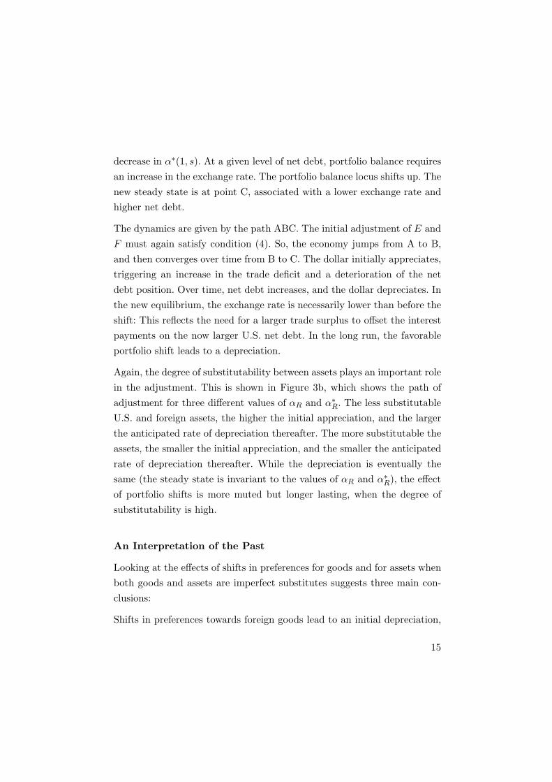
The dynamics are given by the path ABC. The initial adjustment of E andF must again satisfy condition (4). So, the economy jumps from A to B,and then converges over time from B to C. The dollar initially appreciates,triggering an increase in the trade deficit and a deterioration of the netdebt position. Over time, net debt increases, and the dollar depreciates. Inthe new equilibrium, the exchange rate is necessarily lower than before theshift: This reflects the need for a larger trade surplus to offset the interestpayments on the now larger U.S. net debt. In the long run, the favorableportfolio shift leads to a depreciation.

Again, the degree of substitutability between assets plays an important rolein the adjustment. This is shown in Figure 3b, which shows the path ofadjustment for three different values of αR and α∗R. The less substitutableU.S. and foreign assets, the higher the initial appreciation, and the largerthe anticipated rate of depreciation thereafter. The more substitutable theassets, the smaller the initial appreciation, and the smaller the anticipatedrate of depreciation thereafter. While the depreciation is eventually thesame (the steady state is invariant to the values of αR and α∗R), the effectof portfolio shifts is more muted but longer lasting, when the degree ofsubstitutability is high.

An Interpretation of the Past

Looking at the effects of shifts in preferences for goods and for assets whenboth goods and assets are imperfect substitutes suggests three main con-clusions:

Shifts in preferences towards foreign goods lead to an initial depreciation,

15

followed by further anticipated depreciation. Shifts in preferences towardsU.S. assets lead to an initial appreciation, followed by an anticipated de-preciation.

The empirical evidence suggests that both types of shifts have been at workin the recent past in the United States. The first shift, by itself, would haveimplied a steady depreciation in line with increased trade deficits, while weobserved an initial appreciation. The second shift can explain why theinitial appreciation has been followed by a depreciation. But it attributesthe increase in the trade deficit fully to the initial appreciation, whereasthe evidence is of a large adverse shift in the trade balance even aftercontrolling for the effects of the exchange rate. (This does not do justiceto an alternative, and more conventional, monetary policy explanation,high U.S. interest rates relative to foreign interest rates at the end of the1990s, leading to an appreciation, followed since by a depreciation. Relativeinterest rate differentials seem too small however to explain the movementin exchange rates.)

Both shifts lead eventually to a steady depreciation, a lower exchange ratethan before the shift. This follows from the simple condition that higher netdebt, no matter its origin, requires larger interest payments in steady state,and thus a larger trade surplus. The lower the degree of substitutabilitybetween U.S. and foreign assets, the higher the expected rate of deprecia-tion along the path of adjustment. We appear to have indeed entered thisdepreciation phase in the United States.

2 How Large a Depreciation? A Look at the Numbers

The model is simple enough that one can put in some values for the pa-rameters, and draw the implications for the future. More generally, themodel provides a way of looking at the data, and this is what we do in thissection.

16

Parameter Values

Consider first what we know about portfolio shares: In 2003, U.S. financialwealth, W , was equal to $35 trillion, or about three times U.S. GDP ($11trillion).5 Non–U.S. world financial wealth is harder to assess. Based ona ratio of financial assets to GDP of about 2 for Japan and for Europe,and a GDP for the non–U.S. world of approximately $18 trillion in 2003,a reasonable estimate for W ∗/E is $36 trillion—so roughly the same as forthe United States.6

The net U.S. debt position, F measured at market value, was equal to$2.7 trillion in 2003, up from approximate balance in the early 1990s.7 Byimplication, U.S. assets, X, were equal to W +F = $37.7 trillion (35+2.7),and foreign assets, X∗/E, were equal to W ∗/E − F = $33.3 trillion (36-2.7). Put another way, the ratio of U.S. net debt to U.S. assets, F/X, was7.1% (2.7/37.7); the ratio of U.S. net debt to U.S. GDP was equal to 25%(2.7/11).

In 2003, gross U.S. holdings of foreign assets, at market value, were equalto $8.0 trillion. Together with the value for W , this implies that the shareof U.S. wealth in U.S. assets, α, was equal to 0.77 (1 - 8.0/35). Grossforeign holdings of U.S. assets, at market value, were equal to $10.7 trillion.Together with the value of W ∗/E, this implies that the share of foreignwealth in foreign assets, α∗, was equal to 0.70 (1 - 10.7/36).

To get a sense of the implications of these values for α and α∗, note, fromequation (2) that a transfer of one dollar from U.S. wealth to foreign wealth

5. Source for financial wealth: Flow of Funds Accounts of the United States 1995-2003,Table L100, Board of Governors of the Federal Reserve Board, December 20046. For the Euro Area, financial wealth was about 16 trillion euros in 2003, with a GDPof 7.5 trillion (Source: Europe: ECB Bulletin, February 2005, Table 3.1). For Japan,financial wealth was about 900 trillion yen in 2004, with a GDP of 500 trillion. (Source:Flow of Funds, Bank of Japan website, http://www.boj.or.jp/en/stat/sj/sj.html).7. Source for the numbers in this and the next paragraph: BEA, International Trans-actions, Table 2, International Investment Position of the United States at Year End,1976-2003, October 2004

17

implies a decrease in the demand for U.S. assets of (α + α∗− 1) dollars, or47 cents.8

We would like to know not only the values of these shares, but also theirdependence on the relative rate of return—the value of the derivatives αR

and α∗R . Little is known about these values. Gourinchas and Rey [2004]provide indirect evidence of the relevance of imperfect substitutability byshowing that a combination of the trade deficit and the net debt positionhelp predict a depreciation of the exchange rate (we shall return to theirresults later); this would not be the case under perfect substitutability. It ishowever difficult to go from their results to estimates of αR and α∗R. Thus,when needed below, we shall derive results under alternative assumptionsabout these derivatives.

Table 1 summarizes the relevant numbers.

W W ∗/E X X∗/E F α α∗

$35 $36 $37.5 $33.3 $2.7 0.77 0.70

W, W ∗/E, X, X∗/E, F are in trillions of dollars

The next important parameter in our model is θ, the effect of the exchangerate on the trade balance. The natural starting point here is the MarshallLerner relation:

dD

dExports= [η im − η exp − 1]

dE

E

where ηim and ηexp are respectively the elasticities of imports and exportswith respect to the real exchange rate.

8. Note that this conclusion is dependent on the assumption we make in our modelthat marginal and average shares are equal. This may not be the case.

18

Estimates of the η’s based on estimated U.S. import and export equationsrange quite widely (see the survey by Chinn [2004]). In some cases, the es-timates imply that the Marshall–Lerner condition (the condition that theterm in brackets be positive, so a depreciation improves the trade balance)is barely satisfied. Estimates used in macroeconometric models imply avalue for the term in brackets between 0.5 and 0.9. Put another way, to-gether with the assumption that the ratio of U.S. exports to U.S. GDP isequal to 10%, they imply that a reduction of the ratio of the trade deficitto GDP of 1% requires a depreciation somewhere between 11 and 20%.

One may believe however that measurement error, complex lag structures,and mispecification all bias these estimates downwards. An alternative ap-proach is to derive the elasticities from plausible specifications about util-ity, and the pass-through behavior of firms. Using such an approach, and amodel with non tradable goods, tradable domestic goods, and foreign trad-able goods, Obstfeld and Rogoff [2004] find that a decrease in the tradedeficit to GDP of 1% requires a decrease in the real exchange rate some-where between 7% and 10%—thus, a smaller depreciation than implied bymacroeconometric models.

Which value to use is obviously crucial to assess the scope of the requiredexchange rate adjustment. We choose an estimate for the term in bracketsof 0.7—towards the high range of empirical estimates, but lower than theObstfeld Rogoff elasticities. This estimate, together with an export ratioof 10%, implies that a reduction of the ratio of the trade deficit to GDP of1% requires a depreciation of 15%.

A Simple Exercise

We have argued that a depreciation of the dollar has two effects, a con-ventional one through the trade balance, and the other through valuationeffects. To get a sense of the relative magnitudes of the two, consider the

19

effects of an unexpected depreciation in our model. More specifically, con-sider the effects of an unexpected 15% decrease in E+1 relative to E on netdebt, F+1, in equation (3).

The first effect of the depreciation is to improve the trade balance. Givenour earlier discussion and assumptions, such a depreciation reduces thetrade deficit by 1% of GDP (which is why we chose to look at a depreciationof 15%).

The second effect is to increase the dollar value of U.S. holdings of foreignassets (equivalently, reduce the foreign currency value of foreign holdingsof U.S. assets), and thus reduce the U.S. net debt position. From equation(3) (with both sides divided by U.S. output Y , to make the interpretationof the magnitudes easier), this effect is given by:

dF+1

Y= −(1− α)(1 + r∗)

X − F

Y

dE

E

From above, (1 − α) is equal to 0.23, (X − F )/Y to 3. Assume that r∗ isequal to 4%. The effect of the 15% depreciation is then to reduce the ratioof net debt to GDP by 10 percentage points (0.23 x 1.04 x 3 x 0.15).

This implies that, after the unexpected depreciation, interest paymentsare lower by 4% times 10%, or 0.4% of GDP. Putting things together, a15% depreciation improves the current account balance by 1.4% of GDP,roughly one third of it due to valuation effects.9

It is then tempting at this point to ask what size unexpected depreciationwould lead to a sustainable current account deficit today? Take the actualcurrent account deficit to be about 6%. What the “sustainable” currentaccount deficit is depends on the ratio of net debt to GDP the UnitedStates is willing to sustain and on the growth rate of GDP: If the growth

9. A similar computation is given by Lane and Milesi-Ferretti [2004] for a number ofcountries, although not for the United States.

20

rate of U.S. GDP is equal to g, the U.S. can sustain a current account deficitof gF/Y . Assuming for example a growth rate of 3%, and a ratio of net debtto GDP of 25% (the current ratio, but one which has no particular claimto being the right one for this computation) implies that the United Statescan run a current account deficit of 0.75% while maintaining a constantratio of net debt to GDP. In this case, the depreciation required to shiftfrom the actual to the sustainable current account deficit would be equalto roughly 56% ((6% -0.75%) times (15%/1.4%)).

This is a large number, and despite the uncertainty attached to the under-lying values of many of the parameters, it is a useful number to keep inmind. But one should be clear about the limitations of the computation:

First, the United States surely does not need to shift to sustainable currentaccount balance right away. The rest of the world is still willing to lend toit, if perhaps not at the current rate. The longer the United States waitshowever, the higher the ratio of net debt to GDP, and thus the higher theeventual required depreciation. In this sense, our computation gives a lowerbound on the eventual depreciation.

Second, the computation is based on the assumption that, at a currentexchange rate, the trade deficit will remain as large as it is today. If, forexample, we believed that part of the current trade deficit reflected thecombined effect of recent depreciations and J-curve effects, then the com-putation above would clearly overestimate the required depreciation.

The rest of the section deals with these issues. First, by returning to dynam-ics, to have a sense of the eventual depreciation, and of the rate at whichit may be achieved. Second, by looking at the evidence on the origins ofthe shifts in z and s.

21

Returning to Dynamics

How large is the effect of a given shift in z (or in s) on the accumulationof net debt and on the eventual exchange rate? And how long does it taketo get there?

The natural way to answer these questions is to simulate our model usingthe values of the parameters we derived earlier. This is indeed what thesimulations presented in Figure 2b and 3b the previous section did; we looknow more closely at their quantitative implications.

Both sets of simulations are based on the values of the parameters givenabove. Recognizing the presence of output growth (which we did not allowfor in the model), and rewriting the equation for net debt as an equationfor the ratio of net debt to output, we take the term in front of F in thecurrent account balance relation (3) to stand for the interest rate minusthe growth rate. We choose the interest rate to be 4%, the growth rate tobe 3%, so the interest rate minus the growth rate is equal to 1%. We writethe portfolio shares as:

α(R, s) = a + bR + s, α∗(R, s) = a∗ − bR− s

The simulations show the results for three values of the parameter b, b = 10,b = 1.0, and b = 0.1. A value of b of 1 implies that an increase in theexpected relative return on U.S. assets of 100 basis points increases thedesired shares in U.S. assets by one percentage point.

Figure 2b shows the effects of an increase in z of 1% of U.S. GDP. Figure3b shows the effects of an increase in s of 5%, leading to an increase inα and a decrease in α∗ of 5% at a given relative rate of return. Time ismeasured in years.

Figure 2b leads to two main conclusions. First, the effect of a permanentincrease in z by 1% is to eventually increase the ratio of net debt to GDP

22

by 17%, and require an eventual depreciation of 12.5% (Recall that thelong run effects are independent of the degree of substitutability betweenassets, independent of the value of b). Second, it takes a long time to getthere: The figure is truncated at 50 years; by then the adjustment is notyet complete.

Figure 3b leads to similar conclusions. The initial effect of the increase ins is to lead to an appreciation of the dollar, from 23% if b = 0.1, to 12% ifb = 10. The long run effect of the increase in s is to eventually lead to anincrease in the ratio of U.S. net debt to GDP of 35%, and a depreciationof 15%. But, even after 50 years, the adjustment is far from complete, andthe exchange rate is still above its initial level.

What should one conclude from these exercises? That, under the assump-tions that (1) there are no anticipated changes in z, and in α and α∗, (2)that investors have been and will be rational (the simulations are carriedout under rational expectations), and (3) that there are no surprises, thedollar will depreciate by a large amount, but at a steady and slow rate.There are good reasons to question each of these assumptions, and this iswhere we go next.

A Closer Look at the Trade Deficit

To think about the likely path of z, and thus the path of the trade deficit ata given exchange rate, it is useful to write the trade deficit as the differencebetween exports and the value of imports (in terms of domestic goods):

D(E, z) ≡ exp(E, Z∗, z∗)− E imp(E, Z, z)

We have decomposed z into two components, total U.S. spending Z, and z,shifts in the relative demand for U.S versus foreign goods, at a given level

23

of spending and a given exchange rate. z∗ is similarly decomposed betweenZ∗, and shifts in the relative demand for U.S. versus foreign goods, z∗.

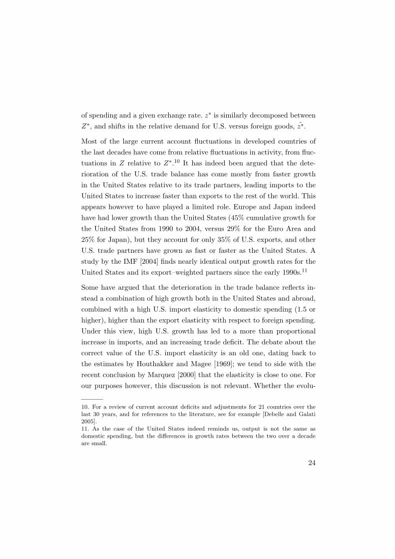
Most of the large current account fluctuations in developed countries ofthe last decades have come from relative fluctuations in activity, from fluc-tuations in Z relative to Z∗.10 It has indeed been argued that the dete-rioration of the U.S. trade balance has come mostly from faster growthin the United States relative to its trade partners, leading imports to theUnited States to increase faster than exports to the rest of the world. Thisappears however to have played a limited role. Europe and Japan indeedhave had lower growth than the United States (45% cumulative growth forthe United States from 1990 to 2004, versus 29% for the Euro Area and25% for Japan), but they account for only 35% of U.S. exports, and otherU.S. trade partners have grown as fast or faster as the United States. Astudy by the IMF [2004] finds nearly identical output growth rates for theUnited States and its export–weighted partners since the early 1990s.11

Some have argued that the deterioration in the trade balance reflects in-stead a combination of high growth both in the United States and abroad,combined with a high U.S. import elasticity to domestic spending (1.5 orhigher), higher than the export elasticity with respect to foreign spending.Under this view, high U.S. growth has led to a more than proportionalincrease in imports, and an increasing trade deficit. The debate about thecorrect value of the U.S. import elasticity is an old one, dating back tothe estimates by Houthakker and Magee [1969]; we tend to side with therecent conclusion by Marquez [2000] that the elasticity is close to one. Forour purposes however, this discussion is not relevant. Whether the evolu-

10. For a review of current account deficits and adjustments for 21 countries over thelast 30 years, and for references to the literature, see for example [Debelle and Galati2005].11. As the case of the United States indeed reminds us, output is not the same asdomestic spending, but the differences in growth rates between the two over a decadeare small.

24

tion of the trade deficit is the result of a high import elasticity or the resultof shifts in the z’s there are no obvious reasons to expect either the shiftto reverse, or growth in the United States to drastically decrease in thefuture.

One way of assessing the relative role of spending, the exchange rate, andother shifts, is to look at the performance of import and export equationsin detailed macroeconometric models. The numbers, using the macroecono-metric model of Global Insight (formerly the DRI model) are as follows:12

The U.S. trade deficit in goods increased from $221 billion in 1998:1 to $674billion in 2004:4. Of this $453 billion increase, $126 billion was due to theincrease in the value of oil imports, leaving $327 billion to be explained.Using the export and import equations of the model, activity variablesand exchange rates explain $202 billion, so about 60% of the increase.Unexplained time trends and residuals account for the remaining 40%, asubstantial amount.13

Looking to the future, whether growth rate differentials, or Houthakker-Magee effects, or unexplained shifts, are behind the increase in the tradedeficit is probably not essential. Lower growth in Europe or in Japan reflectsin large part structural factors, and neither Europe nor Japan are likely tomake up much of the cumulative growth difference since 1995 over the nextfew years. One can still ask how much an increase in growth in Europewould reduce the U.S. trade deficit. A simple computation is as follows.Suppose that Europe and Japan made up the roughly 20% growth gapthey have accumulated since 1990 vis a vis the United States—an unlikelyscenario in the near future—and so U.S. exports to Western Europe and

12. We thank Nigel Gault for communicating these results to us.13. The model has a set of disaggregated export and import equations. Most of the elas-ticities of the different components with respect to domestic or foreign spending are closeto one, so Houthakker-Magee effects play a limited role (except for imports and exportsof consumption goods, where the elasticity of imports with respect to consumption is1.5 for the United States, but the elasticity of exports with respect to foreign GDP is aneven higher 1.9).

25

Japan increased by 20%. Given that U.S. exports to these countries accountfor about 350 billion, the improvement would be 0.7% of U.S. GDP—notnegligible, but not major either.

There is however one place where one may hold more hope for a reductionin the trade deficit, namely the working out of the J- curve. Nominal de-preciations increase import prices, but these decrease imports only with alag. Thus, for a while, depreciations can increase the value of imports andworsen the trade balance, before improving it later. The reason to thinkthis may be important is the “dance of the dollar”, and the joint movementof the dollar and the current account during the 1980s:

From the first quarter of 1979 to the first quarter of 1985, the real exchangerate of the United States (measured by the trade weighted major currenciesindex constructed by the Federal Reserve Board) increased by 41%. Thisappreciation was then followed by a sharp depreciation, with the dollarfalling by 44% from the first quarter of 1985 to the first quarter of 1988.

The appreciation was accompanied by a steady deterioration in the currentaccount deficit, from rough balance in the early 1980s to a deficit of about2.5% when the dollar reached its peak in early 1985. The current accountcontinued to worsen however for more than two years, reaching a peak of3.5% in 1987. The divergent evolutions of the exchange rate and the currentaccount led a number of economists to explore the idea of hysteresis intrade (in particular [Baldwin and Krugman 1987]), the notion that onceappreciation had led to a loss of market shares, an equal depreciation maynot be sufficient to reestablish trade balance. Just as the idea was takinghold, the current account position rapidly improved, and trade was roughlyin balance by the end of the decade.14

14. These issues were discussed at length in the Brookings Papers then. (For exampleCooper [1986], Baldwin and Krugman [1987], Dornbusch [1987], Sachs and Lawrence[1988], with post-mortems by Lawrence [1990] and Krugman [1991].) Another muchdiscussed issue was the respective roles of deficit reduction and exchange rate adjustment.We return to it below.

26

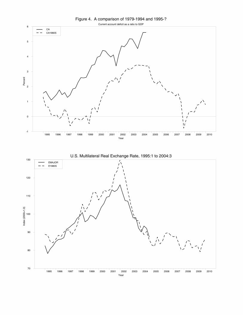
Figure 4. A comparison of 1979-1994 and 1995-?Current account deficit as a ratio to GDP

Year

Per

cent

1995 1996 1997 1998 1999 2000 2001 2002 2003 2004 2005 2006 2007 2008 2009 2010-1

0

1

2

3

4

5

6CA

CA1980S

U.S. Multilateral Real Exchange Rate, 1995:1 to 2004:3

Year

Inde

x (2

000=

1.0)

1995 1996 1997 1998 1999 2000 2001 2002 2003 2004 2005 2006 2007 2008 2009 201070

80

90

100

110

120

130EMAJOR

E1980S

The parallels with current evolutions are clear. They are made even clearerin Figure 4, which plots the evolution of the exchange rate and the currentaccount both during the 1980s and today. The two episodes are aligned sothat the dollar peak of 1985:1 coincides with the dollar peak of 2001:2. Thefigure suggests two conclusions:

If that episode in history is a reliable guide, and the lags similar to thosewhich prevailed in the 1980s, the current account deficit may start to turnaround soon. The deficit is however much larger than it was at its peakin 1987 (6% versus 3.5%) and the depreciation so far has been more lim-ited than in the 1980s (26% from 2001:2 to 2004:4, compared to 39% overthe equivalent period of time from 1985:1 to 1988:3). So one can surelynot conclude that the depreciation so far is enough to get back to a sus-tainable current account deficit. But it may be that in the computationwe went through earlier, one can start from a “J-curve” adjusted currentaccount deficit of 4-5% instead of 6%. If we choose 4%—a very optimisticassumption—then the remaining required depreciation (following the samesteps as we did earlier) is 34% ((4%-0.75%) times (15%/1.4%)).

A Closer Look at Portfolio Shares

One of the striking aspects of the simulations we presented above is howslow the depreciation was along the path of adjustment. This is in contrastwith predictions of much more abrupt falls in the dollar in the near future(for example [Roubini and Setser 2005]). This raises two issues: Can theanticipated depreciation be higher than in the simulations? Are there sur-prises under which the depreciation might be much faster (slower), and ifso which ones? We take both questions in turn.

To answer the first, we go back to the model. We noted earlier that theanticipated rate of depreciation is higher, the lower the degree of substi-tutability between assets. So, by assuming zero substitutability—i.e. con-

27

stant shares, except for changes coming from shifts in s—we can derivean upper bound on the anticipated rate of depreciation. Differentiatingequation (2) gives:

dE

E= −(α + α∗ − 1)X

(1− α∗)X∗/Ed (

F

X) +

(X − F ) dα + (X∗/E + F ) dα∗

(1− α∗)X∗/E

In the absence of anticipated shifts in shares—so the second term is equalto zero—the anticipated rate of depreciation depends on the change in theratio of U.S. net debt to U.S. assets: The faster the increase in net debt,the faster the decrease in the relative demand for U.S. assets, therefore thehigher the rate of depreciation needed to maintain portfolio balance. Usingthe parameters we constructed earlier, this equation implies:

dE

E= −1.6 d (

F

X) + 3.0 (dα− dα∗)

Suppose shares remain constant. If we take the annual increase in the ratioof net debt to U.S. GDP to be 5%, and the ratio of U.S. GDP to U.S.assets to be one third, this gives an anticipated annual rate of depreciationof 2.7% a year (1.6 times .05 divided by 3).15

If, however, shares in U.S. assets in the portfolios of either domestic orforeign investors are expected to decline, the anticipated depreciation canclearly be much larger. If for example, we anticipate the shares of U.S.assets in foreign portfolios to decline by 2% over the coming year, thenthe anticipated depreciation is 8.7% (2.7% from above, plus 3.0 times 2%).This is obviously an upper bound, as it assumes that the remaining in-

15. While a comparison is difficult, this rate appears lower than the rate of deprecia-tion implied by the estimates of Gourinchas and Rey [2004]. Their results imply that acombination of net debt and trade deficits two standard deviations from the mean—asituation which would appear to characterize well the United States today—implies ananticipated annual rate of depreciation of about 5% over the following two years.

28

vestors are willing to keep a constant share of their wealth in U.S. assetsdespite a large negative expected rate of return. Still, it implies that, underimperfect substitutability, and under the assumption that desired shares inU.S. assets will decrease, it is a logically acceptable statement to predict asubstantial depreciation of the dollar in the near future.

Are there good reasons to anticipate these desired shares to decrease in thenear future? This is the subject of a contentious debate:

Some argue that the United States can continue to finance current accountdeficits at the current level for a long time to come, at the same exchangerate. They argue that poor development of financial markets in Asia andelsewhere, and the need to accumulate international collateral, implies asteadily increasing relative demand for U.S. assets. They point to the latentdemand by Chinese private investors, currently limited by capital controls.In short, they argue that foreign investors will be willing to further increase(1 − α∗(R)), and/or that domestic investors will be willing to further in-crease α(R) for many years to come (for example, Dooley et al [2004],Caballero et al [2004]).

Following this argument, we can ask what increase in shares—say, whatincrease in (1 − α∗), the foreign share falling on U.S. assets—would beneeded to absorb the current increase in net debt at a given exchange rate.From the relation derived above, putting dE/E and dα equal to zero gives:

dα∗ = −(α∗ + α− 1)XX∗/E + F

d (F

X)

For the parameters we have constructed, this implies an increase in theshare of U.S. assets in foreign portfolios of about 2.5% a year (0.47 times5%), a large increase by historical standards.16

16. A related argument is that, to the extent that the rest of the world is growing fasterthan the United States, an increase in the ratio of net debt to GDP in the United States

29

We find more plausible the arguments that the relative demand for U.S.assets may actually decrease rather than increase in the future. This isbased in particular on the fact that much of the recent accumulation ofU.S. assets has taken the form of accumulation of reserves by the Japaneseand the Chinese central banks. Many worry that this will not last, that thepegging of the renminbi will come to an end, or that both central bankswill want to change the composition of their reserves away from U.S. assets,leading to further depreciation of the dollar. Our model provides a simpleway of discussing the issue and thinking about the numbers.

Consider pegging first. Pegging means that the foreign central bank buysdollar assets so as keep E = E.17 Let B denote the reserves (i.e the U.S.assets) held by the foreign central bank, so

X = B + α(1)(X − F ) + (1− α∗(1))(X∗

E+ F )

The dynamics under pegging are characterized in Figure 5. Suppose that,in the absence of pegging, the steady state is given by point A, and thatthe foreign central bank pegs the exchange rate at level E. At E, the U.S.current account is in deficit, and so F increases over time. Wealth getssteadily transfered to the foreign country, so the private demand for U.S.assets steadily decreases. To keep E unchanged, B must increase furtherover time. Pegging by the foreign central bank is thus equivalent to a con-tinuous outward shift in the portfolio balance schedule: What the foreigncentral bank is effectively doing is keeping world demand for U.S. assets un-

is consistent with a constant share of its portfolio in U.S. assets. The argument falls quan-titatively short. While Asian countries are growing fast, their weight and their financialwealth are still too small to absorb the U.S. current account deficit while maintainingconstant shares of U.S. assets in their portfolios.17. Our two-country model has only one foreign central bank, and so we cannot discusswhat happens if one foreign bank pegs and the others do not. The issue is howeverrelevant in thinking about the joint evolutions of the dollar–euro and the dollar–yenexchange rates. More on this in the next section.

30

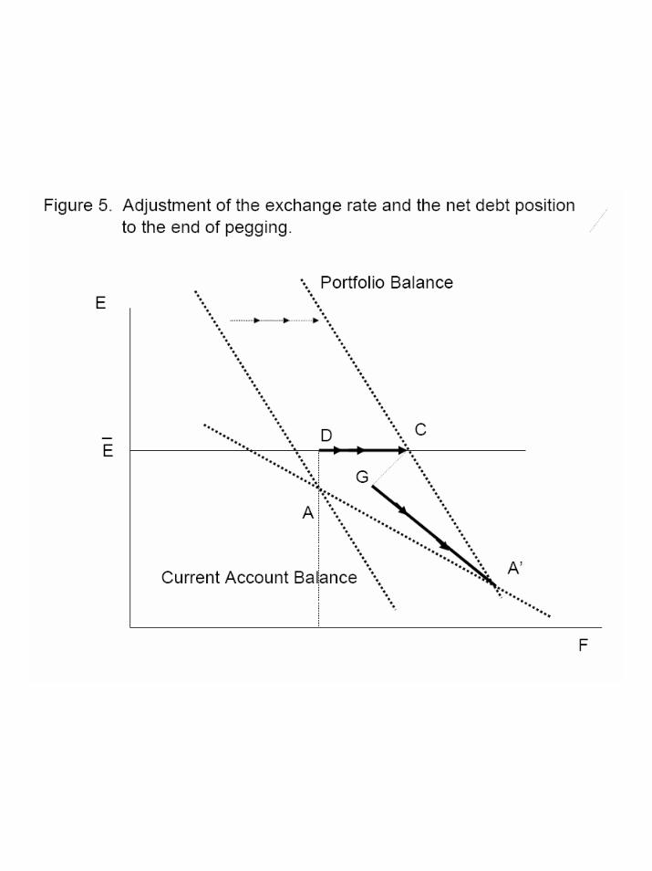
changed by offsetting the fall in private demand. Pegging leads to a steadyincrease in U.S. net debt, and a steady increase in reserves offsetting thesteady decrease in private demands for U.S. assets. This path is representedby the path DC in Figure 5. What happens when the foreign central bank(unexpectedly) stops pegging? The adjustment is represented in Figure 5.With the economy at point C just before the abandon of the peg, theeconomy jumps to G (recall that valuation effects lead to a decrease in netdebt—and therefore a capital loss for the foreign central bank—when thereis an unexpected depreciation), and the economy then adjusts along thesaddle point path DA′. The longer the peg lasts, the larger the initial andthe eventual depreciation.

In other words, an early end to the Chinese peg will obviously lead to adepreciation of the dollar (an appreciation of the renminbi). But the soonerit takes place, the smaller the required depreciation, both initially, and inthe long run. Put another way, the longer the Chinese wait to abandon thepeg, the larger the eventual appreciation of the renminbi.

The conclusions are very similar with respect to changes in the compo-sition of reserves. We can think of such changes as changes in portfoliopreferences, this time not by private investors but by central banks, so wecan apply our earlier analysis directly. A shift away from U.S. assets willlead to an initial depreciation, leading to a lower current account deficit, asmaller increase in net debt, and thus to a smaller depreciation in the longrun.

How large might these shifts be? Chinese reserves are currently equal to500 billion, Japanese reserves to 850 billion. Assuming that these reservesare now held mostly in dollars, and the People’s Bank of China (PBCfor short) and the Bank of Japan (BOJ) reduced their dollar holdings tohalf of their portfolio, this would represent a decrease in the share of U.S.assets in foreign (private and central bank) portfolios, (1− α∗), from 30%to 28%. The computations we presented earlier suggest that this would be

31

a substantial shift, leading to a decrease in the dollar possibly as large as8.7%.

To summarize: To avoid a depreciation of the dollar would require a steadyand substantial increase in shares of U.S. assets in U.S. or foreign portfoliosat a given exchange rate. This seems unlikely to hold for very long. Amore likely scenario is the opposite, a decrease in shares due in particularto diversification of reserves by central banks. If and when this happens,the dollar will depreciate. Note however that the larger the adverse shift,the larger initial depreciation, but the smaller the accumulation of debtthereafter, and therefore the smaller the eventual depreciation. “Bad news”on the dollar now may well be good news in the long run (and the otherway around).

The Path of Interest Rates

We took interest rates as given in our model, and have taken them asconstant so far in our discussion. Yield curves in the United States, Europe,and Japan indeed indicate little expected change in interest rates over thenear and medium term. It is however easy to think of scenarios whereinterest rates may play an important role, and this takes us to an issue wehave not discussed until now, the role of budget deficit reduction in theadjustment process.

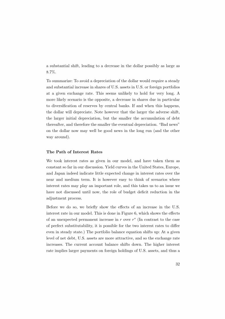
Before we do so, we briefly show the effects of an increase in the U.S.interest rate in our model. This is done in Figure 6, which shows the effectsof an unexpected permanent increase in r over r∗ (In contrast to the caseof perfect substitutability, it is possible for the two interest rates to differeven in steady state.) The portfolio balance equation shifts up: At a givenlevel of net debt, U.S. assets are more attractive, and so the exchange rateincreases. The current account balance shifts down. The higher interestrate implies larger payments on foreign holdings of U.S. assets, and thus a

32

larger trade surplus, a lower exchange rate. The adjustment path is givenby ABC. In response to the increase in r, the economy jumps from A toB, and then moves over time from B to C. As drawn, the exchange rateinitially appreciates, but, in general, the initial effect on the exchange rateis ambiguous: If gross liabilities are large for example, then the effect ofhigher interest payments on the current account balance may dominatethe more conventional “overshooting” effects of increased attractivenessand lead to an initial depreciation rather than an appreciation. In eithercase, the steady state effect is higher net debt accumulation, and thus alarger depreciation than if r had not increased.

Thus, under the assumption that an increase in interest rates leads initiallyto an appreciation, an increase in U.S. interest rates beyond what is alreadyimplicit in the yield curve would delay the depreciation of the dollar, at thecost of higher net debt accumulation, and a larger eventual depreciation.

A more relevant scenario however may be what happens in response toother shifts, for example in response to adverse portfolio shifts leading,at given interest rates, to a large depreciation of the dollar. As the dollardepreciates, relative demand shifts towards U.S. goods, reducing the tradedeficit, but also increasing the total demand for U.S. goods. Suppose alsothat initially output is at its natural level, i.e. the level associated with thenatural rate of unemployment—which appears to be a good description ofthe United States today. Three outcomes are possible:

• Interest rates and fiscal policy remain unchanged. The increase indemand leads to an increase in output, and an increase in importswhich partly offsets the effect of the depreciation on the trade bal-ance. (In terms of our model, it leads to an increase in domesticspending, Z, and thus to a shift in z.)

• Interest rates remain unchanged but fiscal policy is adjusted to offsetthe increase in demand and leave output at its natural level; inother words, the budget deficit is reduced so as to maintain internal

33

balance.• Fiscal policy remains unchanged but the Fed increases interest rates

so as to maintain output at its natural level. In this case, higher U.S.interest rates limit the extent of the depreciation and reduce thecurrent account deficit reduction. In doing so, they lead however tolarger net debt accumulation, and to a larger eventual depreciation.

In short, an orderly reduction of the current account deficit—that is, a de-crease in the current account deficit while maintaining internal balance—requires both a decrease in the exchange rate and a reduction in budgetdeficits.18 The two are not substitutes: The exchange rate depreciation isneeded to achieve current account balance, and the budget deficit reduc-tion is needed to maintain internal balance at the natural level of output.19

(Frequently heard statements that deficit reduction would reduce the needfor a dollar depreciation leave us puzzled). If the depreciation is not ac-companied by a reduction in budget deficits, one of two things can happen:An increase in demand, and the risk that the U.S. economy overheats. Or,and more likely, an increase in U.S. interest rates so as to maintain in-ternal balance. This increase would either limit or delay the depreciationof the dollar. As we have made clear, this is however a mixed blessing.Such a delay implies less depreciation in the short run, but more net debtaccumulation and more depreciation in the long run.

18. Many of the discussions at Brookings in the late 1980s were about the respectiveroles of budget deficit reduction and exchange rate adjustment. To take two examples:Sachs [1988] argued “the budget deficit is the most important source of the trade deficit.Reducing the budget deficit would help reduce the trade deficit [ while] an attempt toreduce the trade deficit by a depreciating exchange rate induced by easier monetary policywould produce inflation with little benefit on the current account”, a view consistentwith the third scenario above. Cooper [1986] in a discussion of the policy package bettersuited to eliminate the U.S. imbalances stated: “The drop in the dollar is an essentialpart of the policy package. The dollar’s decline will help offset the fiscal contractionthrough expansion of net exports and help maintain overall U.S. economic activity at asatisfactory level”, a view consistent with the second scenario.19. A similar point is emphasized by Obstfeld and Rogoff [2004].

34

3 The Euro, the Yen, and the Renminbi

So far, the real depreciation of the dollar since the peak of 2002, has beenvery unevenly distributed: 45 per cent against the Euro, 25 per cent againstthe Yen, zero against the Renminbi. In this section we return to the ques-tions asked in the introduction: If substantially more depreciation is tocome, against which currencies will the dollar fall? If China abandons thepeg, or if Asian banks diversify their reserves, how will the euro and theyen be affected?

The basic answer is simple. Along the adjustment path, what matters—because of home bias in asset preferences—is the reallocation of wealthacross countries, and thus the bilateral current account balances of theUnited States vis a vis its partners. Wealth transfers modify the rela-tive world demands for assets, thus requiring corresponding exchange ratemovements. Other things equal, countries with larger trade surpluses vis avis the United States will see a larger appreciation of their currency.

Other things may not be equal however. Depending on portfolio prefer-ences, a transfer of wealth from the United States to Japan for examplemay change the relative demand for Euro assets, and thus the euro ex-change rate. In that context, one can think of central banks as investorswith different asset preferences. For example, a central bank that holdsmost of its reserves in dollars can be thought of as an investor with strongdollar preferences. Any increase in its reserves is likely to lead to an increasein the relative demand for dollar assets, and thus an appreciation of thedollar. Any diversification of its reserves is likely to lead to a depreciationof the dollar.

There is no way we can construct and simulate a realistic multi-countryportfolio model in this paper. But we can make some progress in thinkingabout mechanisms and magnitudes. The first step is to extend our modelto allow for more countries.

35

Extending the Portfolio Model to Four Regions

In 2004, the U.S. trade deficit in goods (the only category for which adecomposition of the deficit by country is available) was $652 billion. Ofthis, $160 was with China, $75 billion with Japan, $71 with the Euro area,and the remainder with the rest of the world.

We shall ignore the rest of the world here, and think of the world as com-posed of four countries (regions), the United States (indexed 1), Europe(indexed 2), Japan (indexed 3), and China (indexed 4). We shall thereforethink of China as accounting for roughly one half of the U.S. current ac-count deficit, and Europe and Japan as accounting each for roughly onefourth.

We extend our portfolio model as follows. We assume that the share ofasset j in the portfolio of country i is given by

αij(.) = aij + βj({Ri})

where the Ris is the expected gross real rate of return, in dollars, fromholding assets of country i (so Ri denotes a rate of return, not a relativerate of return as in our two-country model). Note that this specificationimplies that differences in portfolio preferences across countries show uponly as different constant terms, while derivatives with respect to rates ofreturn are the same across countries.

The following restrictions apply: From the budget constraint, it follows that∑

j aij = 1 and∑

j βj(.) = 0. The home bias assumption takes the form:∑

i aii > 1. The βj(.) functions are assumed to be homogenous of degreezero in expected gross rates of return.

Domestic interest rates, in domestic currency, are assumed to be equaland constant, all equal to (1 + r). Exchange rates, Ei, are defined as theprice of U.S. goods in terms of foreign goods (so E1 = 1). It follows that

36

the expected gross real rate of return, in dollars, from holding assets ofcountry i is given by Ri = (1 + r)Ei/Ee

i,+1.

In steady state, Ri = (1 + r)Ei/Eei,+1 = (1 + r), so βj({Ri}i) = 0 and

we can concentrate on the aij s. The portfolio balance conditions, absentcentral bank intervention, are given by:

Xj

Ej=

∑

i

aij (Xi

Ei− Fi)

where Fi denotes the net foreign debt position of country i, so∑

i Fi = 0.

So far, we have treated all four countries symmetrically. China is howeverspecial in two dimensions: It enforces strict capital controls, and pegs theexchange rate between the renminbi and the dollar. We capture these twofeatures as follows:

• We formalize capital controls as the assumption that a4i = ai4 = 0for all i 6= 4, i.e. capital controls prevent Chinese residents frominvesting in foreign assets, but also prevent investors outside Chinafrom acquiring Chinese assets.20

• To peg the exchange rate (E4 = 1), the PBC passively acquires allthe dollars flowing into China: the wealth transfer from the U.S. tothe Euro area and Japan is thus the U.S. current account minus thefraction that is financed by the PBC: dF1 + dF4 = −dF2 − dF3.

Some Simple Computations

Assume that a share γ of the U.S. net debt is held by China. Assume theremaining portion is held by the Euro area and Japan according to sharesx and(1− x), so

20. This ignores FDI inflows into China, but since we are considering the financing ofthe U.S. current account deficit, this assumption is inconsequential for our analysis.

37

dF2 = −x(1− γ)dF1, dF3 = −(1− x)(1− γ)dF1, dF4 = −γdF1

Assume that China imposes capital controls and pegs the renminbi. Assumethat the remaining three countries are of the same size, and that the matrixof aij is symmetric in the following way. aii = a and aij = b = (1− a)/2 <

a for i 6= j. In other words, investors want to put more than one third oftheir portfolio into domestic assets (the conditions above imply a > 1/3)and allocates the rest of their portfolio equally among foreign assets.21

Under these assumptions, dE4 = 0 (because of pegging) and dE2 and dE3

are given by:

dE2

dF= −(a− b)(1− γ)[x(1− a) + b(1− x)]

(1− a)2 − b2+

bγ

1− a− b

dE3

dF= −(a− b)(1− γ)[xb + (1− a)(1− x)]

(1− a)2 − b2+

bγ

1− a− b

Consider first the effects of γ. The higher γ, the smaller the appreciationof the euro and the yen vis a vis the dollar. This is hardly surprising:the higher γ, the smaller the transfer of wealth from the United States toEurope and to Japan, thus the smaller the pressure on the euro or the yento appreciate. The interesting term however is the first. To see why, considerthe case where γ = 1, so net debt accumulation is only vis a vis China. Inthis case, the euro and the yen depreciate vis a vis the dollar! This result issurprising but the explanation is straightforward, and is found in portfoliopreferences. The transfer of wealth from the United States to China is atransfer of wealth from U.S. investors, who are willing to hold dollar, euroand yen assets, to the PBC, who only holds dollars. This transfer to an

21. The assumption of equal size countries allows us to specify the matrix in a simpleway. Allowing countries to differ in size—as they obviously do—would lead to a morecomplex size adjusted matrix; but the results we derive below would be unaffected.

38

investor with extreme dollar preferences leads to a relative increase in thedemand for dollars, an appreciation of the dollar vis a vis the euro and theyen.

Consider now the effects of x. For simplicity, put γ equal to zero. Considerfirst the case where x = 0, so the trade deficit is entirely vis a vis Japan.In this case, it follows that dE3 = 2 dE2. Both the yen and the euroappreciate vis a vis the dollar, with the yen appreciating twice as much asthe euro. This result might again be surprising: Why should a transfer ofwealth from the United States to Japan lead to a change in the relativedemand for euros? The answer is that it does not. The euro goes up visa vis the dollar, but down vis a vis the yen. The real effective exchangerate of the euro remains unchanged. If x = 1/2, which seems to correspondroughly the ratio of trade deficits today, then obviously the euro and theyen appreciate in the same proportion vis a vis the dollar.

This simple framework also allows us to think what would happen if Chinastopped pegging, and/or diversified its reserves away from dollars, and/orrelaxed capital controls on Chinese and foreign investors.

Suppose China stopped pegging, while maintaining capital controls. Givencapital controls, the renminbi would have to appreciate vis a vis the dollarin order to eliminate the trade deficit vis a vis the United States. From thenon, reserves of the PBC would remain constant. So as the United Statescontinued to accumulate net debt vis a vis Japan and Europe, relativenet debt vis a vis China would decrease. In terms of our model, γ—theproportion of U.S. net debt held by China—would decrease.22 Building onour results, this would lead to a decrease in the role of an investor withextreme preferences, namely the PBC, and would lead to an appreciationof the euro and the yen. Suppose instead that China diversified its reservesaway from dollars. Then, again, the demand for euros and for yens would

22. Marginal γ, the proportion of the increase in U.S. net debt falling on China, wouldbe equal to zero.

39

increase, leading to an appreciation of the euro and the yen vis a vis thedollar.

To summarize: The trade deficits vis a vis Japan and the Euro area implyan appreciation of both currencies vis a vis the dollar. This effect is partiallyoffset by the Chinese policies of pegging and keeping most of its reservesin dollars. If China were to give up its peg, or diversify its reserves, theeuro and the yen would appreciate further vis a vis the dollar. This lastargument is at odds with an often heard statement that the Chinese peghas “increased the pressure on the euro” and that therefore, the abandonof the peg would remove some of the pressure, leading to a depreciation ofthe euro. We do not understand the logic behind that statement.

Two Simulations and a Look at Portfolios

We have looked so far at equilibrium for a given distribution of F s. Thisdistribution is endogenous in our model, determined by trade deficits andportfolio preferences. We now show the result of a simulation of our ex-tended model.

The assumptions are as follows. We consider a shift in the U.S. trade deficit,falling for one half on China, for one fourth on Japan, and for one fourth onthe Euro area. We assume that each country only trades with the UnitedStates, so we can focus on the bilateral balances with the United States. Theparameters are the same for all countries. We do the simulation under twoalternative assumptions about China. In both, we assume capital controls.In the first, we assume that China pegs the renminbi. In the second, weassume that the renminbi floats; together with the assumption of capitalcontrols, this implies a zero Chinese trade deficit.

The results are shown in Figure 7. Because of symmetry, the response ofthe euro and the yen are identical, and thus represented by the same line.The bottom line shows the depreciation of the dollar vis a vis the euro

40

Figure 7. The effects of a U.S. trade shock on the Euro/$ and the Yen/$ exchange rates, with or without Chinese peg.

Response of the Exchange Rate to a Trade Shock

-0.06

-0.05

-0.04

-0.03

-0.02

-0.01

0

1 4 7 10 13 16 19 22 25 28 31 34 37 40 43 46

Time

Exc

hang

e R

ate

(pro

port

iona

l dev

iatio

n)

Pegging with capital controls Floating with capital controls

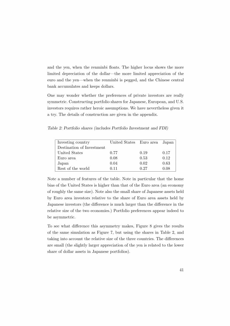
and the yen, when the renminbi floats. The higher locus shows the morelimited depreciation of the dollar—the more limited appreciation of theeuro and the yen—when the renminbi is pegged, and the Chinese centralbank accumulates and keeps dollars.

One may wonder whether the preferences of private investors are reallysymmetric. Constructing portfolio shares for Japanese, European, and U.S.investors requires rather heroic assumptions. We have nevertheless given ita try. The details of construction are given in the appendix.

Table 2: Portfolio shares (includes Portfolio Investment and FDI)

Investing country United States Euro area JapanDestination of InvestmentUnited States 0.77 0.19 0.17Euro area 0.08 0.53 0.12Japan 0.04 0.02 0.63Rest of the world 0.11 0.27 0.08

Note a number of features of the table. Note in particular that the homebias of the United States is higher than that of the Euro area (an economyof roughly the same size). Note also the small share of Japanese assets heldby Euro area investors relative to the share of Euro area assets held byJapanese investors (the difference is much larger than the difference in therelative size of the two economies.) Portfolio preferences appear indeed tobe asymmetric.

To see what difference this asymmetry makes, Figure 8 gives the resultsof the same simulation as Figure 7, but using the shares in Table 2, andtaking into account the relative size of the three countries. The differencesare small (the slightly larger appreciation of the yen is related to the lowershare of dollar assets in Japanese portfolios).

41

Figure 8. The effects of a U.S. trade shock on the Euro/$ and the Yen/$ exchange rates, with or without Chinese peg. (using actual portfolio shares)

Response of the Exchange Rate to a Trade Shock

-0.07

-0.06

-0.05

-0.04

-0.03

-0.02

-0.01

0

1 3 5 7 9 11 13 15 17 19 21 23 25 27 29 31 33 35 37 39 41 43 45 47

Time

Exch

ange

Rat

e (p

ropo

rtio

nal d

evia

tion)

dollar-euro (Pegging with capital controls) dollar-yen (Pegging with capital controls)dollar-euro (Floating with capital controls) dollar-yen (Floating with capital controls)

Summary and Conclusions

We have argued that there have been two main forces behind the largeU.S. current account deficits which have developed over the past 10 years:an increase in the U.S. demand for foreign goods and an increase in theforeign demand for U.S. assets. The path of the dollar since the late 1990’scan be explained as the reaction to these shocks.

The shift in portfolio preferences towards U.S. assets came first (in the late1990s) in the form of a high private demand for U.S. equities, more recentlyin the form of high central bank demands for U.S. bonds.

The shift in demand away from U.S. goods is often related to higher growthin the U.S. relative to its trading partners. This appears however to haveplayed only a limited role: the performance of import and export equationsin macroeconometric models shows that activity variables and exchangerates explain only about 60% of the increase in the U.S. trade deficit:Unexplained time trends and residuals account for the remaining 40%. Weinterpret this as evidence of a shift in the U.S. trade balance.

Either shift could only have induced the path of the dollar and the U.S.current account that we have experienced in a world where financial assetsare imperfect substitutes. The shift in asset preferences, because it wouldbe meaningless in a world where assets are perfect substitutes. The shift inthe U.S. trade balance, because with perfect substitutability such a shift—provided it were perceived as long lasting—would have induced a quickerand stronger depreciation of the exchange rate, and a smaller increase inthe current account.

To organize thoughts about the U.S. current account deficit and the dollarwe have thus studied a simple model characterized by imperfect substi-tutability both among goods and among assets. The model allows for valu-ation effects, whose relevance has recently been emphasized in a number ofpapers: The explicit integration of valuation effects in a model of imperfect

42

substitutability is, we believe, novel.

We find that the degree of substitutability between assets does not affectthe steady state. In other words, the eventual dollar depreciation inducedby either shift is the same no matter how close substitutes U.S. and foreignassets are. But the degree of substitutability plays a central role in thedynamics of adjustment.

In contrast to the case of perfect substitutability between assets, an in-crease in the U.S. demand for foreign goods leads to a limited depreciationinitially, a potentially large and long lasting current account deficit, anda slow and steady depreciation over time. An increase in the foreign de-mand for U.S. assets leads to an initial appreciation, followed by a slowand steady depreciation thereafter.

The slow rate of dollar depreciation implied by imperfect substitutabilityis in contrast with many predictions of much more abrupt falls in the dollarin the near future. We show that in the absence of anticipated portfolioshifts, the anticipated rate of depreciation depends on the change in theratio of U.S. net debt to U.S. assets: The faster the increase in net debt,the faster the decrease in the relative demand for U.S. assets, therefore thehigher the rate of depreciation needed to maintain portfolio balance. If wetake the annual increase in the ratio of net debt to U.S. GDP to be 5%,we derive an upper bound on the anticipated annual rate of depreciationof 2.7% a year.

If shares in U.S. assets in the portfolios of either U.S. or foreign investorsare instead expected to decline, the anticipated depreciation can be muchlarger. If for example, we anticipate the shares of U.S. assets in foreignportfolios to decline by 2% over the coming year, then the upper boundon the anticipated depreciation is 8.7%. This is obviously only an upperbound, derived by assuming that the remaining investors are willing tokeep a constant share of their wealth in U.S. assets despite a large negative

43

rate of return. Still, it implies that, under imperfect substitutability, andunder the assumption that desired shares in U.S. assets will decrease, itis a logically acceptable statement to predict a substantial depreciation ofthe dollar in the near future.

On the contrary, a further shift in investors’ preferences towards dollarassets would slow down, or even reverse, the path of dollar depreciation.The relief, however, would only be temporary. It would lead to an initialappreciation, but the accompanying loss of competitiveness would speed upthe accumulation of foreign debt. The long run value of the dollar wouldbe even lower. Thus the argument that the United States, thanks to theattractiveness of its assets, can keep running large current account deficitswith no effect on the dollar, appears to overlook the long run consequencesof a large accumulation of external liabilities.

For basically the same reason, an increase in interest rates would be selfdefeating. It might temporarily strengthen the dollar, but the depreciationeventually needed to restore equilibrium in the current account would beeven larger—both because (as in the case of a shift in portfolio preferences)the accumulation of foreign liabilities would accelerate, and because even-tually the U.S. would need to finance a larger flow of interest paymentsabroad. A better mix would be a decrease in interest rates, and a reduc-tion in budget deficits to avoid overheating. (To state the obvious: Tighterfiscal policy is needed to reduce the current account deficit, but is not asubstitute for the dollar depreciation. Both are needed.)

The same will happen so long as China keeps pegging the exchange rate.One should think of the PBC as a special investor whose presence hasthe effect of raising the portfolio share that the rest of the world investsin dollar assets. The longer the PBC intervenes, the higher the share ofrest-of-world wealth invested in U.S. assets. Sooner or later, however—asin the case of Korea in the late 1980’s—the PBC will find it increasinglydifficult to sterilize the accumulation of reserves. Eventually, when the peg

44

is abandoned, the depreciation of the dollar will be larger the longer thepeg will have lasted, because in the process the U.S. will have accumulatedlarger quantities of foreign liabilities. Thus, if China is worried by a loss ofcompetitiveness, pegging may be a myopic choice.

What would an abandonment of the peg imply for the Euro and the Yen?Contrary to a common argument, when the Renminbi is left to float, bothcurrencies are likely to appreciate further relative to the dollar. The reasonis that, when the PBC stops intervening, the market effectively loses aninvestor with extreme dollar preferences, who will be replaced by privateinvestors with less extreme preferences. A similar argument holds if thePBC diversifies its reserves away from dollar assets.

For Europe and Japan, however, what matters are effective exchange ratesand these may well depreciate even if the bilateral dollar exchange rateappreciates.

We end with one more general remark. A large fall in the dollar is notby itself a catastrophe for the United States. It leads to higher demandand higher output, and it offers the opportunity to reduce budget deficitswithout triggering a recession. The danger is much more serious for Japanand Western Europe, although it would be alleviated by an abandonmentof the Chinese peg.

45

Appendix 1. Dynamics of the Model

The dynamics of the system composed of equations (2) and (3) are moreeasily characterized by taking the continuous time limit. In continuoustime, the portfolio and current account balance equations become:

X = α(1+ r− r∗+Ee

E, s) (X −F )+ (1−α∗(1+ r− r∗+

Ee

E), s) (

X∗

E+F )

F = rF + (1− α(1 + r + r∗ +Ee

E), s)

E

E(X − F ) + D(E, z)

Note the presence of both expected and actual depreciation in the currentaccount balance relation. Expected appreciation determines the share ofthe U.S. portfolio put in foreign assets; actual appreciation determines thechange in the value of that portfolio, and in turn the change in the U.S.net debt position.

We limit ourselves to a characterization of the equilibrium and local dy-namics, using a phase diagram. (Global dynamics are more complex. Thenon linearities imbedded in the equations imply that the economy is likelyto have two equilibria, only one of them potentially saddle point stable.This is the equilibrium we focus on.) We do so here under the additionalassumption that r = r∗. The extension to different interest rates, which weuse to construct Figure 6 in the text, is straightforward.

The locus (E = Ee = 0) is obtained from the portfolio balance equation,and is downward sloping: In the presence of home bias, an increase innet debt shifts wealth abroad, decreasing the demand for U.S. assets, andrequiring a depreciation.

The locus (F = 0) is obtained by assuming (Ee = E) in the current accountbalance relation and replacing (Ee) by its implied value from the portfolio

46

balance equation. This locus is also downward sloping: A depreciation leadsto a smaller trade deficit, and thus allows for a larger net debt positionconsistent with current account balance.

Note that the locus (F = 0) is not the same as the current account balancelocus in Figure 1 in the text; that locus is derived under the assumptionthat both the F and E are equal to zero.

The derivatives αR and α∗R do not affect the slope of the E = 0 locus. Theydo however affect the slope of the F = 0. The smaller these derivatives (thelower the degree of substitutability between assets), the closer the locus(F = 0) is to the (E = 0). In the limit, if the degree of substitutabilitybetween U.S. and foreign assets is equal to zero, the two loci coincide. Thelarger these derivatives (the higher the degree of substitutability betweenassets), the closer the (F = 0) locus is to the current account balance locus:0 = rF + D(E).

The condition for the equilibrium to be saddle point stable is that the locus(E = 0) be steeper than the (F = 0) locus (which turns out to be the sameas the condition given in the text, that the portfolio balance relation besteeper than the current account balance relation). For this to hold, thefollowing condition must be satisfied:

r

EDE<

α + α∗ − 1(1− α∗)X∗/E

The interpretation was given in the text. The condition is more likely tobe satisfied, the lower the interest rate, the larger the home bias, and thelarger the response of the trade balance to the exchange rate. If the condi-tion is satisfied, the dynamics are as shown in Figure A1. The saddle path isdownward sloping, implying that the adjustment to the steady state frombelow is associated with an expected depreciation, the adjustment fromabove with an expected appreciation. Valuation effects imply that unex-

47

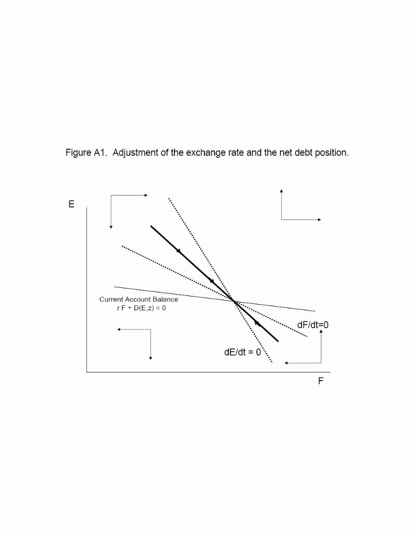
pected shifts in z or s are associated with initial changes in F , accordingto:

∆F = (1− α)(1 + r∗)(X − F )∆E

E

The effect of the degree of substitutability on the dynamics is as follows:

The smaller αR and α∗R, the closer the locus (F = 0) is to the (E = 0), andso the closer the saddle point path is to the (E = 0). In the limit, if thedegree of substitutability between U.S. and foreign assets is equal to zero,the two loci and the saddle point path coincide, and the economy remainson and adjusts along the (E = 0), the portfolio balance relation.

The larger αR and α∗R, the closer the (F = 0) locus is to the locus givenby 0 = rF + D(E), and the closer the saddle point path is to that locusas well. Also the larger αR and α∗R, the slower the adjustment of F and E

over time. The slow adjustment of F comes from the fact that we are closeto current account balance. The slow adjustment of E comes from the factthat, the larger the elasticities, the smaller is E for a given distance fromthe E = 0 locus.

The limiting case of perfect substitutability is degenerate. The rate of ad-justment to (unexpected, permanent) shifts in z goes to zero. The economyis always on the locus 0 = rF + D(E). For any level of net debt, the ex-change rate adjusts so net debt remains constant, and, in the absence ofshocks, the economy stays at that point. There is no unique steady state,and where the economy is depends on history.

Appendix 2. Construction of the Shares

The portfolio shares underlying Table 1 refer both to portfolio investmentnarrowly defined and to foreign direct investment positions.

48

Data on the country allocation of gross portfolio investments are from theIMF Coordinated Portfolio Survey for 2002. Data for the country allocationof direct investment are from the OECD and also refer to 2002. Financialwealth for the USA, the Euro area and Japan, which we need to computethe home bias of portfolios, are from the Flow of Funds.23

The aij are then constructed in two steps. First we compute the geograph-ical allocation of net foreign investment positions by weighting the share ofportfolio assets and fdi’s allocated to country j by the relative importanceof portfolio and direct investment in country i’s total investments abroad.We then scale these shares by the share of total foreign investment (1−aii),so that

aij = [(pfi/(pfi + fdii)) aij,p + (fdii/(pfi + fdii))aij,fdi] ∗ (1− ajj)

23. Source for Japan: http://www.boj.or.jp/en/stat/sj/sj.html); for theEuro area, ECB Economic Bulletin (released February, 2005), orhttp://www.ecb.int/pub/html/index.en.html).

49

References

[Baldwin and Krugman1987] Baldwin, R. and Krugman, P., 1987, Thepersistence of the u.s. trade deficit, Brookings Papers on Economic Ac-

tivity 1, 1–55.[Caballero et al.2004] Caballero, R., Farhi, E., and Hammour, M., 2004,

Speculative growth: Hints from the U.S. economy, mimeo, MIT.[Chinn2004] Chinn, M., 2004, Incomes, exchange rates and the U.S. trade

deficit, once again, International Finance 7(3), 451–469.[Cooper] Cooper, R., Dealing with the trade deficit in a floating rate

system, Brookings Papers on Economic Activity.[Debelle and Galati2005] Debelle, G. and Galati, G., 2005, Current ac-

count adjustment and capital flows, BIS working papers (169), Monetaryand Economic Department, Bank of International Settlements.

[Dornbusch1976] Dornbusch, R., 1976, Expectations and exchange ratedynamics, Journal of Political Economy 84, 1161–1176.

[Gourinchas and Rey2004] Gourinchas, P.-O. and Rey, H., 2004, Interna-tional financial adjustment, mimeo, Berkeley.

[Henderson and Rogoff1982] Henderson, D. and Rogoff, K., 1982, Negativenet foreign asset positions and stability in a world portfolio balancemodel, Journal of International Economics 13, 85–104.

[Hooper et al.2001] Hooper, P., Johnson, P., and Marguez, J., 2001, Tradeelasticities for the G7 countries, Princeton Studies in International Fi-

nance 87.[Houthakker and Magee1969] Houthakker, H. and Magee, S., 1969, Income

and price elasticities in world trade, Review of Economics and Statistics

51(1), 111–125.[International Monetary Fund2004] International Monetary Fund, 2004,

U.S. selected issues, Article IV United States Consultation-Staff Report.[Kouri1976] Kouri, P., 1976, Capital flows and the dynamics of the ex-

50

change rate, Seminar paper 67, Institute for International EconomicStudies, Stockholm.

[Kouri1983] Kouri, P., 1983, Balance of payments and the foreign exchangemarket: A dynamic partial equilibrium model, pp. 116–156, in Economic

Interdependence and Flexible Exchange Rates, J. Bhandari and B. Put-nam eds, MIT Press, Cambridge, Mass.

[Krugman1991] Krugman, P., 1991, Introduction, pp. 1–13, in “Inter-national Adjustment and Financing”, Fred Bergsten ed, Institute forInternational Economics, Washington D.C.

[Lane and Milesi-Ferretti2002] Lane, P. and Milesi-Ferretti, G., 2002, Longterm capital movements, NBER Macroeconomics Annual pp. 73–115.

[Lane and Milesi-Ferretti2004] Lane, P. and Milesi-Ferretti, G., 2004, Fi-nancial globalization and exchange rates, CEPR DP 4745.

[Lawrence and Hooper1990] Lawrence, R. and Hooper, P., 1990, U.S. cur-rent account adjustment: An appraisal, Brookings Papers on Economic

Activity 2, 343–392.[Mann1999] Mann, C., 1999, Is the U.S. trade deficit sustainable?, Institute

for International Economics, Washington.[Marquez2000] Marquez, J., 2000, The puzzling income elasticity of U.S.

imports, mimeo, Federal Reserve Board.[Obstfeld2004] Obstfeld, M., 2004, External adjustment, Review of World

Economics 140(4), 541–568.[Obstfeld and Rogoff2004] Obstfeld, M. and Rogoff, K., 2004, The unsus-

tainable U.S. current account revisited, 10869, NBER Working Paper.[Sachs and Lawrence1988] Sachs, J. and Lawrence, R., 1988, Global ad-

justment to a shrinking U.S. trade deficit, Brookings Papers on Economic

Activity 2, 639–674.

51