14.452 Economic Growth: Overlapping Generations · 14.452 Economic Growth: Lecture 7, Overlapping...

14.452 Economic Growth: Lecture 7, Overlapping Generations

Daron Acemoglu

MIT

November 17, 2009.

Daron Acemoglu (MIT) Economic Growth Lecture 7 November 17, 2009. 1 / 54

Growth with Overlapping Generations Growth with Overlapping Generations

Growth with Overlapping Generations

In many situations, the assumption of a representative household is not appropriate because

1

2

households do not have an infinite planning horizon new households arrive (or are born) over time.

New economic interactions: decisions made by older “generations” will affect the prices faced by younger “generations”. Overlapping generations models

1

2

3

4

5

Capture potential interaction of different generations of individuals in the marketplace; Provide tractable alternative to infinite-horizon representative agent models; Some key implications different from neoclassical growth model; Dynamics in some special cases quite similar to Solow model rather than the neoclassical model; Generate new insights about the role of national debt and Social Security in the economy.


Growth with Overlapping Generations Problems of Infinity

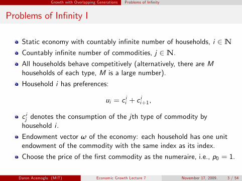
Problems of Infinity I

Static economy with countably infinite number of households, i ∈ N

Countably infinite number of commodities, j ∈ N.

All households behave competitively (alternatively, there are M households of each type, M is a large number).

Household i has preferences:

ui = cii + ci i +1,

icj denotes the consumption of the jth type of commodity by household i .

Endowment vector ω of the economy: each household has one unit endowment of the commodity with the same index as its index.

Choose the price of the first commodity as the numeraire, i.e., p0 = 1.



Problems of Infinity II

Proposition In the above-described economy, the price vector p̄ such that p̄j = 1 for all j ∈ N is a competitive equilibrium price vector and induces an equilibrium with no trade, denoted by x̄ .

Proof:

At p̄, each household has income equal to 1. Therefore, the budget constraint of household i can be written as

cii + ci

i +1 ≤ 1.

This implies that consuming own endowment is optimal for each household, Thus p̄ and no trade, x̄ , constitute a competitive equilibrium.



Problems of Infinity III

However, this competitive equilibrium is not Pareto optimal. Consider alternative allocation, x̃ :

Household i = 0 consumes its own endowment and that of household 1. All other households, indexed i > 0, consume the endowment of than neighboring household, i + 1. All households with i > 0 are as well off as in the competitive equilibrium (p̄, x̄). Individual i = 0 is strictly better-off.

Proposition In the above-described economy, the competitive equilibrium at (p̄, x̄) is not Pareto optimal.



Problems of Infinity IV

Source of the problem must be related to the infinite number of commodities.

Extended version of the First Welfare Theorem covers infinite number ∗of commodities, but only assuming ∑∞

j =0 pj ωj < ∞ (written with the aggregate endowment ωj ).

∗Here theonly endowment is labor, and thus p = 1 for all j ∈ N, so j∗that ∑j

∞ =0 pj ωj = ∞ (why?).

This abstract economy is “isomorphic” to the baseline overlapping generations model.

The Pareto suboptimality in this economy will be the source of potential ineffi ciencies in overlapping generations model.



Problems of Infinity V

∗Second Welfare Theorem did not assume ∑∞ =0 pj ωj < ∞.j

Instead, it used convexity of preferences, consumption sets and production possibilities sets.

This exchange economy has convex preferences and convex consumption sets:

Pareto optima must be decentralizable by some redistribution of endowments.

Proposition In the above-described economy, there exists a reallocation of the endowment vector ω to ~ω, and an associated competitive equilibrium (p̄, x̃) that is Pareto optimal where x̃is as described above, and p̄ is such that p̄j = 1 for all j ∈ N.



Proof of Proposition

Consider the following reallocation of ω: endowment of household i ≥ 1 is given to household i − 1.

At the new endowment vector ~ = 0 has one unit of good ω, household i j = 0 and one unit of good j = 1. Other households i have one unit of good i + 1.

At the price vector p̄, household 0 has a budget set

c00 + c1 ≤ 2,1

0 0thus chooses c = c = 1.0 1

All other households have budget sets given by

cii + ci

i +1 ≤ 1,

Thus it is optimal for each household i > 0 to consume one unit of the good ci i +1 Thus x̃ is a competitive equilibrium.


The Baseline OLG Model Environment

The Baseline Overlapping Generations Model

Time is discrete and runs to infinity.

Each individual lives for two periods.

Individuals born at time t live for dates t and t + 1.

Assume a general (separable) utility function for individuals born at date t,

U (t) = u (c1 (t)) + βu (c2 (t + 1)) , (1)

u : R+ → R satisfies the usual Assumptions on utility.

c1 (t): consumption of the individual born at t when young (at date t).

c2 (t + 1): consumption when old (at date t + 1).

β ∈ (0, 1) is the discount factor.



Demographics, Preferences and Technology I

Exponential population growth,

L (t) = (1 + n)t L (0) . (2)

Production side same as before: competitive firms, constant returns to scale aggregate production function, satisfying Assumptions 1 and 2:

Y (t) = F (K (t) , L (t)) .

Factor markets are competitive.

Individuals can only work in the first period and supply one unit of labor inelastically, earning w (t).



Demographics, Preferences and Technology II

Assume that δ = 1.

k ≡ K /L, f (k) ≡ F (k, 1), and the (gross) rate of return to saving, which equals the rental rate of capital, is

1 + r (t) = R (t) = f � (k (t)) , (3)

As usual, the wage rate is

w (t) = f (k (t)) − k (t) f � (k (t)) . (4)


The Baseline OLG Model Consumption Decisions

Consumption Decisions I

Savings by an individual of generation t, s (t), is determined as a solution to

max c1 (t),c2 (t+1),s(t)

u (c1 (t)) + βu (c2 (t + 1))

subject to c1 (t) + s (t) ≤ w (t)

and c2 (t + 1) ≤ R (t + 1) s (t) ,

Old individuals rent their savings of time t as capital to firms at time t + 1, and receive gross rate of return R (t + 1) = 1 + r (t + 1)

Second constraint incorporates notion that individuals only spend money on their own end of life consumption (no altruism or bequest motive).



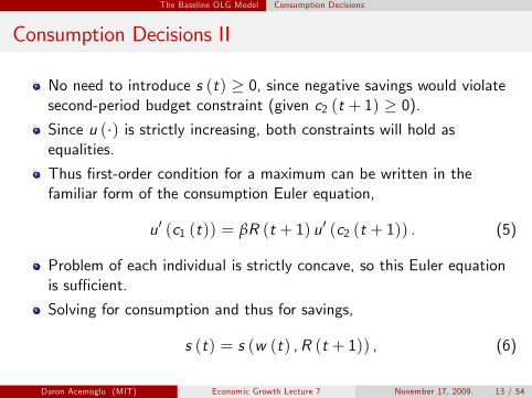
Consumption Decisions II

No need to introduce s (t) ≥ 0, since negative savings would violate second-period budget constraint (given c2 (t + 1) ≥ 0).

Since u (·) is strictly increasing, both constraints will hold as equalities.

Thus first-order condition for a maximum can be written in the familiar form of the consumption Euler equation,

u� (c1 (t)) = βR (t + 1) u� (c2 (t + 1)) . (5)

Problem of each individual is strictly concave, so this Euler equation is suffi cient.

Solving for consumption and thus for savings,

s (t) = s (w (t) , R (t + 1)) , (6)



Consumption Decisions III

s : R2 → R is strictly increasing in its first argument and may be + increasing or decreasing in its second argument.

Total savings in the economy will be equal to

S (t) = s (t) L (t) ,

L (t) denotes the size of generation t, who are saving for time t + 1.

Since capital depreciates fully after use and all new savings are invested in capital,

K (t + 1) = L (t) s (w (t) , R (t + 1)) . (7)


The Baseline OLG Model Equilibrium

Equilibrium I

Definition A competitive equilibrium can be represented by a sequence of aggregate capital stocks, individual consumption and factor prices,

∞{K (t) , c1 (t) , c2 (t) , R (t) , w (t)} =0, such that the factor t∞price sequence {R (t) , w (t)} =0 is given by (3) and (4), t ∞individual consumption decisions {c1 (t) , c2 (t)} =0 are tgiven by (5) and (6), and the aggregate capital stock,

∞{K (t)} =0, evolves according to (7). t

Steady-state equilibrium defined as usual: an equilibrium in which k ≡ K /L is constant. To characterize the equilibrium, divide (7) by L(t + 1) = (1 + n) L (t),

s (w (t) , R (t + 1)) k (t + 1) = .

1 + n



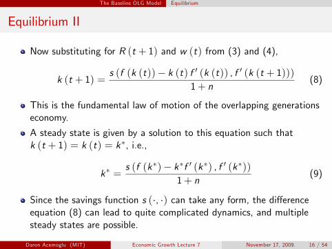
Equilibrium II

Now substituting for R (t + 1) and w (t) from (3) and (4),

s (f (k (t)) − k (t) f � (k (t)) , f � (k (t + 1))) k (t + 1) = (8)

1 + n

This is the fundamental law of motion of the overlapping generations economy.

A steady state is given by a solution to this equation such that k (t + 1) = k (t) = k∗, i.e.,

s (f (k∗) − k∗f � (k∗) , f � (k∗)) k∗ = (9)

1 + n

Since the savings function s (·, ·) can take any form, the difference equation (8) can lead to quite complicated dynamics, and multiple steady states are possible.



Equilibrium III


Courtesy of Princeton University Press. Used with permission.Fig. 9.1 in Acemoglu, Daron. Introduction to Modern Economic Growth.Princeton, NJ: Princeton University Press, 2009. ISBN: 9780691132921.

http://press.princeton.edu/titles/8764.html

� �

The Baseline OLG Model Special Cases

Restrictions on Utility and Production Functions I

Suppose that the utility functions take the familiar CRRA form:

1−θ 1−θ c1 (t) − 1 c2 (t + 1) − 1U (t) = + β , (10)

1 − θ 1 − θ

where θ > 0 and β ∈ (0, 1).

Technology is Cobb-Douglas,

f (k) = kα

The rest of the environment is as described above.

The CRRA utility simplifies the first-order condition for consumer optimization,

c2 (t + 1) 1/θ= (βR (t + 1)) . c1 (t)



Restrictions on Utility and Production Functions II

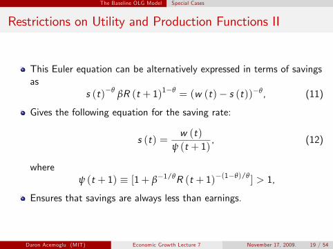
This Euler equation can be alternatively expressed in terms of savings as

−θ 1−θ s (t) βR (t + 1) = (w (t) − s (t))−θ , (11)

Gives the following equation for the saving rate:

w (t)s (t) =

ψ (t + 1) , (12)

where −(1−θ)/θψ (t + 1) ≡ [1 + β−1/θR (t + 1) ] > 1,

Ensures that savings are always less than earnings.


� �


Restrictions on Utility and Production Functions III

The impact of factor prices on savings is summarized by the following and derivatives:

∂s (t) 1 sw ≡ = ∈ (0, 1) ,

∂w (t) ψ (t + 1) ∂s (t) 1 − θ −1/θ s (t)

sR ≡ = (βR (t + 1)) . ∂R (t + 1) θ ψ (t + 1)

Since ψ (t + 1) > 1, we also have that 0 < sw < 1.

Moreover, in this case sR > 0 if θ > 1, sR < 0 if θ < 1, and sR = 0 if θ = 1.

Refiects counteracting infiuences of income and substitution effects.

Case of θ = 1 (log preferences) is of special importance, may deserve to be called the canonical overlapping generations model.



Restrictions on Utility and Production Functions IV

Equation (8) implies

s(t)k (t + 1) = (13)

(1 + n) w (t)

=(1 + n)ψ (t + 1)

,

Or more explicitly,

f (k (t)) − k (t) f � (k (t)) k (t + 1) = (14)−(1−θ)/θ(1 + n) [1 + β−1/θf � (k(t + 1)) ]

The steady state then involves a solution to the following implicit equation:

f (k∗) − k∗f � (k∗)k∗ = .

(1 + n) [1 + β−1/θf �(k∗)−(1−θ)/θ ]


� �


Restrictions on Utility and Production Functions V

Now using the Cobb-Douglas formula, steady state is the solution to the equation � � �(θ−1)/θ

� (1 + n) 1 + β−1/θ α(k∗ )α−1 = (1 − α)(k∗ )α−1 . (15)

For simplicity, define R∗ ≡ α(k∗)α−1 as the marginal product of capital in steady-state, in which case, (15) can be rewritten as

1 − α(θ−1)/θ(1 + n) 1 + β−1/θ (R∗ ) = R∗ . (16)α

Steady-state value of R∗, and thus k∗, can now be determined from equation (16), which always has a unique solution. To investigate the stability, substitute for the Cobb-Douglas production function in (14)

α(1 − α) k (t)k (t + 1) = . (17)−(1−θ)/θ(1 + n) [1 + β−1/θ (αk(t + 1)α−1) ]



Restrictions on Utility and Production Functions VI

Proposition In the overlapping-generations model with two-period lived households, Cobb-Douglas technology and CRRA preferences, there exists a unique steady-state equilibrium with the capital-labor ratio k∗ given by (15), this steady-state equilibrium is globally stable for all k (0) > 0.

In this particular (well-behaved) case, equilibrium dynamics are very similar to the basic Solow model

Figure shows that convergence to the unique steady-state capital-labor ratio, k∗, is monotonic.


Canonical OLG Model Canonical Model

Canonical Model I

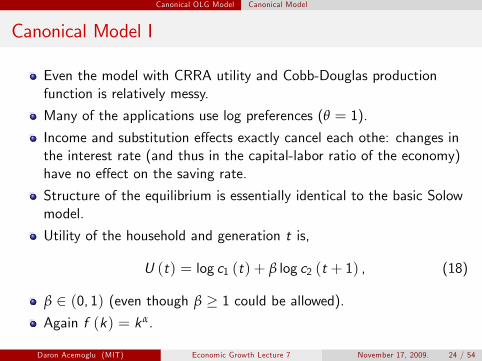
Even the model with CRRA utility and Cobb-Douglas production function is relatively messy.

Many of the applications use log preferences (θ = 1).

Income and substitution effects exactly cancel each othe: changes in the interest rate (and thus in the capital-labor ratio of the economy) have no effect on the saving rate.

Structure of the equilibrium is essentially identical to the basic Solow model.

Utility of the household and generation t is,

U (t) = log c1 (t) + β log c2 (t + 1) , (18)

β ∈ (0, 1) (even though β ≥ 1 could be allowed).

Again f (k) = kα .



Canonical Model II

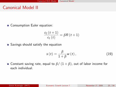
Consumption Euler equation:

c2 (t + 1) = βR (t + 1)

c1 (t)

Savings should satisfy the equation

β s (t) = w (t) , (19)

1 + β

Constant saving rate, equal to β/ (1 + β), out of labor income for each individual.



Canonical Model III

Combining this with the capital accumulation equation (8),

s(t)k (t + 1) =

(1 + n) βw (t)

= (1 + n) (1 + β)

αβ (1 − α) [k(t)]=

(1 + n) (1 + β) ,

Second line uses (19) and last uses that, given competitive factor αmarkets, w (t) = (1 − α) [k(t)] .

There exists a unique steady state with � � 1 β (1 − α) 1−α

k∗ = . (20)(1 + n) (1 + β)

Equilibrium dynamics are identical to those of the basic Solow model and monotonically converge to k∗ .



45°

k*

k*k(0) k’(0)0

k(t+1)

k(t)

Figure: Equilibrium dynamics in the canonical overlapping generations model.


Courtesy of Princeton University Press. Used with permission.Fig. 9.2 in Acemoglu, Daron. Introduction to Modern Economic Growth.Princeton, NJ: Princeton University Press, 2009. ISBN: 9780691132921.

http://press.princeton.edu/titles/8764.html


Canonical Model IV

Proposition In the canonical overlapping generations model with log preferences and Cobb-Douglas technology, there exists a unique steady state, with capital-labor ratio k∗ given by (20). Starting with any k (0) ∈ (0, k∗), equilibrium dynamics are such that k (t) ↑ k∗, and starting with any k � (0) > k∗ , equilibrium dynamics involve k (t) ↓ k∗ .


Overaccumulation and Policy Overaccumulation and Pareto Optimality

Overaccumulation I

Compare the overlapping-generations equilibrium to the choice of a social planner wishing to maximize a weighted average of all generations’utilities.

Suppose that the social planner maximizes

βt SU (t) t=0

βS is the discount factor of the social planner, which refiects how she values the utilities of different generations.

∞

∑



Overaccumulation II

∞

∑

Substituting from (1), this implies:

βtS (u (c1 (t)) + βu (c2 (t + 1))) t=0

subject to the resource constraint

F (K (t) , L (t)) = K (t + 1) + L (t) c1 (t) + L (t − 1) c2 (t) .

Dividing this by L (t) and using (2),

c2 (t)f (k (t)) = (1 + n) k (t + 1) + c1 (t) + .1 + n



Overaccumulation III

Social planner’s maximization problem then implies the following first-order necessary condition:

u� (c1 (t)) = βf � (k (t + 1)) u� (c2 (t + 1)) .

Since R (t + 1) = f � (k (t + 1)), this is identical to (5).

Not surprising: allocate consumption of a given individual in exactly the same way as the individual himself would do.

No “market failures” in the over-time allocation of consumption at given prices.

However, the allocations across generations may differ from the competitive equilibrium: planner is giving different weights to different generations

In particular, competitive equilibrium is Pareto suboptimal when k∗ > kgold ,



Overaccumulation IV

When k∗ > kgold , reducing savings can increase consumption for every generation.

More specifically, note that in steady state

∗ −1 ∗f (k∗ ) − (1 + n)k∗ = c1 + (1 + n) c2 ∗≡ c ,

First line follows by national income accounting, and second defines ∗ c .

Therefore ∗ ∂c = f � (k∗ ) − (1 + n)

∂k∗

kgold is defined as f � (kgold ) = 1 + n.



Overaccumulation V

Now if k∗ > kgold , then ∂c ∗/∂k∗ < 0: reducing savings can increase (total) consumption for everybody.

If this is the case, the economy is referred to as dynamically ineffi cient– it involves overaccumulation.

Another way of expressing dynamic ineffi ciency is that

∗ r < n,

Recall in infinite-horizon Ramsey economy, transversality condition required that r > g + n.

Dynamic ineffi ciency arises because of the heterogeneity inherent in the overlapping generations model, which removes the transversality condition.

Suppose we start from steady state at time T with k∗ > kgold .



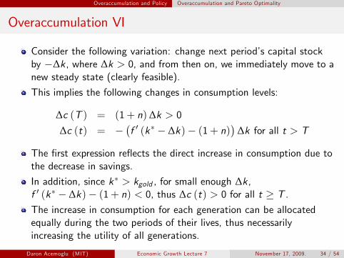
Overaccumulation VI

Consider the following variation: change next period’s capital stock by −Δk, where Δk > 0, and from then on, we immediately move to a new steady state (clearly feasible).

This implies the following changes in consumption levels:

Δc (T ) = (1 + n) Δk > 0

Δc (t) = − � f � (k∗ − Δk) − (1 + n)

� Δk for all t > T

The first expression refiects the direct increase in consumption due to the decrease in savings.

In addition, since k∗ > kgold , for small enough Δk, f � (k∗ − Δk) − (1 + n) < 0, thus Δc (t) > 0 for all t ≥ T .

The increase in consumption for each generation can be allocated equally during the two periods of their lives, thus necessarily increasing the utility of all generations.



Pareto Optimality and Suboptimality in the OLG Model

Proposition In the baseline overlapping-generations economy, the competitive equilibrium is not necessarily Pareto optimal.

∗More specifically, whenever r < n and the economy is dynamically ineffi cient, it is possible to reduce the capital stock starting from the competitive steady state and increase the consumption level of all generations.

Pareto ineffi ciency of the competitive equilibrium is intimately linked with dynamic ineffi ciency.



Interpretation

Intuition for dynamic ineffi ciency:

Individuals who live at time t face prices determined by the capital stock with which they are working. Capital stock is the outcome of actions taken by previous generations. Pecuniary externality from the actions of previous generations affecting welfare of current generation. Pecuniary externalities typically second-order and do not matter for welfare. But not when an infinite stream of newborn agents joining the economy are affected. It is possible to rearrange in a way that these pecuniary externalities can be exploited.



Further Intuition

Complementary intuition:

Dynamic ineffi ciency arises from overaccumulation. Results from current young generation needs to save for old age. However, the more they save, the lower is the rate of return and may encourage to save even more. Effect on future rate of return to capital is a pecuniary externality on next generation If alternative ways of providing consumption to individuals in old age were introduced, overaccumulation could be ameliorated.


Overaccumulation and Policy Role of Social Security

Role of Social Security in Capital Accumulation

Social Security as a way of dealing with overaccumulation

Fully-funded system: young make contributions to the Social Security system and their contributions are paid back to them in their old age.

Unfunded system or a pay-as-you-go: transfers from the young directly go to the current old.

Pay-as-you-go (unfunded) Social Security discourages aggregate savings.

With dynamic ineffi ciency, discouraging savings may lead to a Pareto improvement.


Overaccumulation and Policy Fully Funded Social Security

Fully Funded Social Security I

Government at date t raises some amount d (t) from the young, funds are invested in capital stock, and pays workers when old R (t + 1) d (t).

Thus individual maximization problem is,

max c1 (t),c2 (t+1),s(t)

u (c1 (t)) + βu (c2 (t + 1))

subject to c1 (t) + s (t) + d (t) ≤ w (t)

and c2 (t + 1) ≤ R (t + 1) (s (t) + d (t)) ,

for a given choice of d (t) by the government.

Notice that now the total amount invested in capital accumulation is s (t) + d (t) = (1 + n) k (t + 1).



Fully Funded Social Security II

No longer the case that individuals will always choose s (t) > 0. ∞As long as s (t) is free, whatever {d (t)} =0, the competitive t

equilibrium applies.

When s (t) ≥ 0 is imposed as a constraint, competitive equilibrium ∞ ∞applies if given {d (t)} =0, privately-optimal {s (t)} =0 is such that t t

s (t) > 0 for all t.



Fully Funded Social Security III

Proposition Consider a fully funded Social Security system in the above-described environment whereby the government collects d (t) from young individuals at date t.

1 Suppose that s (t) ≥ 0 for all t. If given the feasible ∞ sequence {d (t)} =0 of Social Security payments, the t ∞utility-maximizing sequence of savings {s (t)} =0 ist

such that s (t) > 0 for all t, then the set of competitive equilibria without Social Security are the set of competitive equilibria with Social Security.

2 Without the constraint s (t) ≥ 0, given any feasible ∞ sequence {d (t)} =0 of Social Security payments, the t

set of competitive equilibria without Social Security are the set of competitive equilibria with Social Security.

Moreover, even when there is the restriction that s (t) ≥ 0, a funded Social Security program cannot lead to the Pareto improvement.


Overaccumulation and Policy Unfunded Social Security

Unfunded Social Security I

Government collects d (t) from the young at time t and distributes to the current old with per capita transfer b (t) = (1 + n) d (t) Individual maximization problem becomes

max c1 (t),c2 (t+1),s(t)

u (c1 (t)) + βu (c2 (t + 1))

subject to c1 (t) + s (t) + d (t) ≤ w (t)

and c2 (t + 1) ≤ R (t + 1) s (t) + (1 + n) d (t + 1) ,

for a given feasible sequence of Social Security payment levels ∞{d (t)}t=0.

Rate of return on Social Security payments is n rather than r (t + 1) = R (t + 1) − 1, because unfunded Social Security is a pure transfer system.



Unfunded Social Security II

Only s (t)– rather than s (t) plus d (t) as in the funded scheme– goes into capital accumulation.

It is possible that s (t) will change in order to compensate, but such an offsetting change does not typically take place.

Thus unfunded Social Security reduces capital accumulation.

Discouraging capital accumulation can have negative consequences for growth and welfare.

In fact, empirical evidence suggests that there are many societies in which the level of capital accumulation is suboptimally low.

But here reducing aggregate savings may be good when the economy exhibits dynamic ineffi ciency.



Unfunded Social Security III

Proposition Consider the above-described overlapping generations economy and suppose that the decentralized competitive equilibrium is dynamically ineffi cient. Then there exists a feasible sequence of unfunded Social Security payments

∞{d (t)} =0 which will lead to a competitive equilibrium tstarting from any date t that Pareto dominates the competitive equilibrium without Social Security.

Similar to way in which the Pareto optimal allocation was decentralized in the example economy above.

Social Security is transferring resources from future generations to initial old generation.

But with no dynamic ineffi ciency, any transfer of resources (and any unfunded Social Security program) would make some future generation worse-off.


OLG with Impure Altruism Impure Altruism

Overlapping Generations with Impure Altruism I

Exact form of altruism within a family matters for whether the representative household would provide a good approximation.

Parents care about certain dimensions of the consumption vector of their offspring instead of their total utility or “impure altruism.”

A particular type, “warm glow preferences”: parents derive utility from their bequest.

Production side given by the standard neoclassical production function, satisfying Assumptions 1 and 2, f (k).

Economy populated by a continuum of individuals of measure 1.

Each individual lives for two periods, childhood and adulthood.

In second period of his life, each individual begets an offspring, works and then his life comes to an end.

No consumption in childhood (or incorporated in the parent’s consumption).



Overlapping Generations with Impure Altruism II

No new households, so population is constant at 1.

Each individual supplies 1 unit of labor inelastically during is adulthood.

Preferences of individual (i , t), who reaches adulthood at time t, are

log (ci (t)) + β log (bi (t)) , (21)

where ci (t) denotes the consumption of this individual and bi (t) is bequest to his offspring.

Offspring starts the following period with the bequest, rents this out as capital to firms, supplies labor, begets his own offspring, and makes consumption and bequests decisions.

Capital fully depreciates after use.



Overlapping Generations with Impure Altruism III

Maximization problem of a typical individual can be written as

max log (ci (t)) + β log (bi (t)) , (22) ci (t),bi (t)

subject to

ci (t) + bi (t) ≤ yi (t) ≡ w (t) + R (t) bi (t − 1) , (23)

where yi (t) denotes the income of this individual. Equilibrium wage rate and rate of return on capital

w (t) = f (k (t)) − k (t) f � (k (t)) (24)

R (t) = f � (k (t)) (25)

Capital-labor ratio at time t + 1 is: � 1 k (t + 1) = bi (t) di , (26)

0



Overlapping Generations with Impure Altruism IV

Measure of workers is 1, so that the capital stock and capital-labor ratio are identical. Denote the distribution of consumption and bequests across households at time t by [ci (t)]i ∈[0,1] and [bi (t)]i ∈[0,1].

Assume the economy starts with the distribution of wealth (bequests) � 1at time t given by [bi (0)]i ∈[0,1], which satisfies bi (0) di > 0.0

Definition An equilibrium in this overlapping generations economy with warm glow preferences is a sequence of consumption and bequest levels for each household,� �∞ [ci (t)]i ∈[0,1] , [bi (t)]i ∈[0,1] , that solve (22) subject to

t=0 ∞(23), a sequence of capital-labor ratios, {k (t)} =0, given by t(26) with some initial distribution of bequests [bi (0)]i ∈[0,1],

∞and sequences of factor prices, {w (t) , R (t)} =0, that tsatisfy (24) and (25).



Overlapping Generations with Impure Altruism V

Solution of (22) subject to (23) is straightforward because of the log preferences,

bi (t) = β

1 + β yi (t)

= β

1 + β [w (t) + R (t) bi (t − 1)] , (27)

for all i and t.

Bequest levels will follow non-trivial dynamics.

bi (t) can alternatively be interpreted as “wealth” level: distribution of wealth that will evolve endogenously.

This evolution will depend on factor prices.

To obtain factor prices, aggregate bequests to obtain the capital-labor ratio of the economy via equation (26).



Overlapping Generations with Impure Altruism VI

Integrating (27) across all individuals, � 1 k (t + 1) = bi (t) di

0 � 1β = [w (t) + R (t) bi (t − 1)] di

1 + β 0

β = f (k (t)) . (28)

1 + β � 1The last equality follows from the fact that 0 bi (t − 1) di = k (t) and because by Euler’s Theorem, w (t) + R (t) k (t) = f (k (t)).

Thus dynamics are straightforward and again closely resemble Solow growth model.

Moreover dynamics do not depend on the distribution of bequests or income across households.



Overlapping Generations with Impure Altruism VII

Solving for the steady-state equilibrium capital-labor ratio from (28),

k∗ = β

f (k∗ ) , (29)1 + β

Uniquely defined and strictly positive in view of Assumptions 1 and 2. Moreover, equilibrium dynamics again involve monotonic convergence to this unique steady state. We know that k (t) → k∗, so the ultimate bequest dynamics are given by steady-state factor prices.

∗Let these be denoted by w = f (k∗) − k∗f � (k∗) and R∗ = f � (k∗). Once the economy is in the neighborhood of the steady-state capital-labor ratio, k∗ ,

∗bi (t) = β

[w + R∗bi (t − 1)] .1 + β



Overlapping Generations with Impure Altruism VIII

When R∗ < (1 + β) /β, starting from any level bi (t) will converge to a unique bequest (wealth) level

∗ b∗ =

βw . (30)

1 + β (1 − R∗)

Moreover, it can be verified that R∗ < (1 + β) /β,

R∗ = f � (k∗ )

< f (k∗) k∗

1 + β =

β ,

Second line exploits the strict concavity of f (·) and the last line uses the definition of k∗ from (29).



Overlapping Generations with Impure Altruism IX

Proposition Consider the overlapping generations economy with warm glow preferences described above. In this economy, there exists a unique competitive equilibrium. In this equilibrium the aggregate capital-labor ratio is given by (28) and monotonically converges to the unique steady-state capital-labor ratio k∗ given by (29). The distribution of bequests and wealth ultimately converges towards full equality, with each individual having a bequest (wealth) level

∗of b∗ given by (30) with w = f (k∗) − k∗f � (k∗) and R∗ = f � (k∗).


Conclusions Conclusions

Conclusions

Overlapping generations of the more realistic than infinity-lived representative agents. Models with overlapping generations fall outside the scope of the First Welfare Theorem:

they were partly motivated by the possibility of Pareto suboptimal allocations.

Equilibria may be “dynamically ineffi cient” and feature overaccumulation: unfunded Social Security can ameliorate the problem. Declining path of labor income important for overaccumulation, and what matters is not finite horizons but arrival of new individuals. Overaccumulation and Pareto suboptimality: pecuniary externalities created on individuals that are not yet in the marketplace. Not overemhasize dynamic ineffi ciency: major question of economic growth is why so many countries have so little capital.


For information about citing these materials or our Terms of Use, visit: http://ocw.mit.edu/terms.

MIT OpenCourseWare http://ocw.mit.edu

14.452 Economic Growth Fall 2009

For information about citing these materials or our Terms of Use,visit: http://ocw.mit.edu/terms.

http://ocw.mit.edu

http://ocw.mit.edu/terms

14.452 Economic Growth: Overlapping Generations · 14.452 Economic Growth: Lecture 7, Overlapping...

Documents

Transcript of 14.452 Economic Growth: Overlapping Generations · 14.452 Economic Growth: Lecture 7, Overlapping...