The Two-sample Rank-sum Test: … journal articles attribute the origin of the two-sample rank-sum...

Journ@l électronique d’Histoire des Probabilités et de la Statistique/ Electronic Journal for History of Probability and Statistics . Vol.8, Décembre/December 2012

Journ@l Electronique d’Histoire des Probabilités et de la Statistique

Electronic Journ@l for History of Probability and Statistics

Vol 8; Décembre/December 2012

www.jehps.net

The Two-sample Rank-sum Test: Early

DevelopmentKENNETH J. BERRY,1 PAUL W. MIELKE, Jr.,2 and JANIS E.

JOHNSTON3,4

ResumeNous etudions l’histoire du test statistique de la somme des rangs pour un double echantillon. Alorsque la plupart des textes attribuent sa creation a Wilcoxon (1945) ou/et a Mann et Whitney (1947),le test a ete developpe independamment par au moins six chercheurs a la fin des annees 1940 etau debut des annees 1950. En complement de Wilcoxon et Mann et Whitney, Festinger (1946),Whitfield (1947), Haldane and Smith (1948), et van der Reyden (1952) ont publie de facon autonomedes versions equivalentes, quoique differant par leur methodologie, du test du rang. Dans cet article,nous decrivons et comparont le developpement de ces six approches.

AbstractThe historical development of the two-sample rank-sum test is explored. While most textbooksand journal articles attribute the origin of the two-sample rank-sum test to Wilcoxon (1945) and/orMann and Whitney (1947), the test was independently developed by at least six researchers in thelate 1940s and early 1950s. In addition to Wilcoxon and Mann and Whitney, Festinger (1946),Whitfield (1947), Haldane and Smith (1948), and van der Reyden (1952) autonomously publishedmethodologically distinct, but equivalent versions of the two-sample rank-sum test. In this articlethe historical development of the six approaches are described and compared.

Key names: L. Festinger, J. B. S. Haldane, H. B. Mann, D. van der Reyden, C. A. B. Smith, J.W. Whitfield, D. R. Whitney, F. Wilcoxon

Keywords: Combinatoric Methods, History of Statistics, Partitions, Two-sample Rank-sumTest

1Department of Sociology, Colorado State University, Fort Collins, CO 80523–1784, USA. e-mail:[email protected].

2Department of Statistics, Colorado State University, Fort Collins, CO 80523–1877, USA.3Food and Nutrition Service, United States Department of Agriculture, Alexandria, VA 22302–1500, USA.4The views expressed in this article are those of the author and do not necessarily reflect the position or policy

of the United States Department of Agriculture or the United States Government.


1 IntroductionIn the 1930s and 1940s it was widely recognized that when extreme values (outliers) werepresent in sets of data, the assumption of normality underlying conventional parametric testssuch as t tests, analysis of variance, and correlation was untenable and the results were there-fore questionable (cf. Vankeerberghen, Vandenbosch, Smeyers-Verbeke, & Massart, 1991). Inresponse, a number of non-parametric distribution-free counterparts to existing parametric testswere developed, typically based on converting raw measurements to rank values, notwithstand-ing the potential loss of information in reducing numerical values to ranks. Rank tests such asKendall’s measure of rank correlation (Kendall, 1938), Friedman’s two-way analysis of vari-ance by ranks (Friedman, 1937), and the Kruskal–Wallis one-way analysis of variance by ranks(Kruskal & Wallis, 1952) are very robust to outliers (Potvin & Roff, 1993). The non-parametriccounterpart to the two-sample t test is the two-sample rank-sum test based on the sums ofthe ranks in the two samples, independently developed by Wilcoxon (1945), Festinger (1946),Mann and Whitney (1947), Whitfield (1947), Haldane and Smith (1948), and van der Reyden(1952).

The logic underlying the two-sample rank-sum test is straightforward. The data consistof two independent samples drawn from identically distributed populations. Let x1, x2, . . . , xn

denote the first random sample of size n and let y1, y2, . . . , ym denote the second random sampleof size m. Assign the ranks 1 to n + m to the combined observations from smallest to largestwithout regard to sample membership and let Rk denote the rank assigned to the n +m obser-vations for k = 1, . . . , n + m. Let Tx and Ty denote the sums of the ranks from the first andsecond samples, respectively, and let T = Tx. Finally, note that

Tx + Ty =(n+m)(n+m+ 1)

2.

The null hypothesis simply states that each of the possible arrangements of the n + mobservations to the two samples with n values in the first sample and m values in the secondsample occurs with equal probability. The exact lower (upper) one-sided probability value of anobserved value of T , To, is the proportion of all possible

(n+mn

)T values less (greater) than or

equal to To.For example, consider n + m = 10 graduate students in a graduate seminar with n = 5

males and m = 5 females. Fig. 1 contains the raw data where xi and yj represent current agesin years. Fig. 2 lists the numerical ages, sex (M, F), and associated ranks of the n + m = 10

Males: 20, 22, 23, 28, 32Females: 24, 25, 27, 30, 45

Fig. 1: Current ages of n = 5 male and m = 5 female graduate students.

graduate students based on the data in Fig. 1. For the data in Fig. 2, To = Tx = 22, Ty = 33,and only 39 (224) of the

(n+m

n

)=

(n+m)!

n!m!=

(5 + 5)!

5! 5!= 252

2


1 IntroductionIn the 1930s and 1940s it was widely recognized that when extreme values (outliers) werepresent in sets of data, the assumption of normality underlying conventional parametric testssuch as t tests, analysis of variance, and correlation was untenable and the results were there-fore questionable (cf. Vankeerberghen, Vandenbosch, Smeyers-Verbeke, & Massart, 1991). Inresponse, a number of non-parametric distribution-free counterparts to existing parametric testswere developed, typically based on converting raw measurements to rank values, notwithstand-ing the potential loss of information in reducing numerical values to ranks. Rank tests such asKendall’s measure of rank correlation (Kendall, 1938), Friedman’s two-way analysis of vari-ance by ranks (Friedman, 1937), and the Kruskal–Wallis one-way analysis of variance by ranks(Kruskal & Wallis, 1952) are very robust to outliers (Potvin & Roff, 1993). The non-parametriccounterpart to the two-sample t test is the two-sample rank-sum test based on the sums ofthe ranks in the two samples, independently developed by Wilcoxon (1945), Festinger (1946),Mann and Whitney (1947), Whitfield (1947), Haldane and Smith (1948), and van der Reyden(1952).

The logic underlying the two-sample rank-sum test is straightforward. The data consistof two independent samples drawn from identically distributed populations. Let x1, x2, . . . , xn

denote the first random sample of size n and let y1, y2, . . . , ym denote the second random sampleof size m. Assign the ranks 1 to n + m to the combined observations from smallest to largestwithout regard to sample membership and let Rk denote the rank assigned to the n +m obser-vations for k = 1, . . . , n + m. Let Tx and Ty denote the sums of the ranks from the first andsecond samples, respectively, and let T = Tx. Finally, note that

Tx + Ty =(n+m)(n+m+ 1)

2.

The null hypothesis simply states that each of the possible arrangements of the n + mobservations to the two samples with n values in the first sample and m values in the secondsample occurs with equal probability. The exact lower (upper) one-sided probability value of anobserved value of T , To, is the proportion of all possible

(n+mn

)T values less (greater) than or

equal to To.For example, consider n + m = 10 graduate students in a graduate seminar with n = 5

males and m = 5 females. Fig. 1 contains the raw data where xi and yj represent current agesin years. Fig. 2 lists the numerical ages, sex (M, F), and associated ranks of the n + m = 10

Males: 20, 22, 23, 28, 32Females: 24, 25, 27, 30, 45

Fig. 1: Current ages of n = 5 male and m = 5 female graduate students.

graduate students based on the data in Fig. 1. For the data in Fig. 2, To = Tx = 22, Ty = 33,and only 39 (224) of the

(n+m

n

)=

(n+m)!

n!m!=

(5 + 5)!

5! 5!= 252

2

Age: 20, 22, 23, 24, 25, 27, 28, 30, 32, 45Sex: M, M, M, F, F, F, M, F, M, FRank: 1, 2, 3, 4, 5, 6, 7, 8, 9, 10

Fig. 2: Age, sex, and corresponding rank of n = 5 male and m = 5 female graduate students.

Table 1: Listing of the 39 combinations of ranks with T values less than or equal to To = 22.

Number Ranks T Number Ranks T Number Ranks T

1 1 2 3 4 5 15 14 1 2 3 5 9 20 27 1 3 4 6 7 212 1 2 3 4 6 16 15 1 2 3 6 8 20 28 2 3 4 5 7 213 1 2 3 4 7 17 16 1 2 4 5 8 20 29 1 2 3 6 10 224 1 2 3 5 6 17 17 1 2 4 6 7 20 30 1 2 3 7 9 225 1 2 3 4 8 18 18 1 3 4 5 7 20 31 1 2 4 5 10 226 1 2 3 5 7 18 19 2 3 4 5 6 20 32 1 2 4 6 9 227 1 2 4 5 6 18 20 1 2 3 5 10 21 33 1 2 4 7 8 228 1 2 3 4 9 19 21 1 2 3 6 9 21 34 1 2 5 6 8 229 1 2 3 5 8 19 22 1 2 3 7 8 21 35 1 3 4 5 9 22

10 1 2 3 6 7 19 23 1 2 4 5 9 21 36 1 3 4 6 8 2211 1 2 4 5 7 19 24 1 2 4 6 8 21 37 1 3 5 6 7 2212 1 3 4 5 6 19 25 1 2 5 6 7 21 38 2 3 4 5 8 2213 1 2 3 4 10 20 26 1 3 4 5 8 21 39 2 3 4 5 7 22

possible values of T are less (greater) than or equal to To = 22. For clarity, the 39 T values lessthan or equal to To = 22 are listed in Table 1. Thus, for the data in Figs. 1 and 2, the exact lower(upper) one-sided probability of To = 22 is 39/252 .

= 0.1548 (224/252 .= 0.8889).

2 Development of the Two-sample Rank-sum TestStigler’s law of eponymy states that “[n]o scientific discovery is named after its original discov-erer” (Stigler, 1999, p. 277). Stigler observed that names are not given to scientific discoveriesor inventions by historians of science, but by the community of practicing scientists, most ofwhom have no historical expertise. Moreover, the award of an eponym must be made on thebasis of the scientific merit of originality and not upon personal friendship, national affiliation,or political pressure (Stigler, 1999, pp. 280–281).

The two-sample rank-sum test, commonly referenced with the eponym “Wilcoxon–Mann–Whitney test,” was invented and reinvented by a number of researchers in the late 1940s andearly 1950s (considering co-authors as a single contributor): F. Wilcoxon in 1945, L. Festingerin 1946, H. B. Mann and D. R. Whitney in 1947, J. W. Whitfield in 1947, J. B. S. Haldane andC. A. B. Smith in 1948, and D. van der Reyden in 1952. Because Festinger (1946) publishedhis version of the two-sample rank-sum test in Psychometrika, Haldane and Smith (1948) pub-lished their version in The Annals of Eugenics, and van der Reyden (1952) published his version

3


in The Rhodesia Agricultural Journal, their work was largely overlooked by statisticians at thetime. Although Whitfield (1947) published his version in Biometrika, which was widely read bystatisticians, the article contained no references to earlier work on the two-sample rank-sum testand was, in fact, simply an examination of rank correlation between two variables, one dichoto-mous and one ranked, utilizing a pairwise procedure previously developed by M. G. Kendall(1938).

The development of the two-sample rank-sum test has never been adequately documented.In 1957 Kruskal (1957) published a short note titled “Historical notes on the Wilcoxon unpairedtwo-sample test” that discussed early contributions by Deuchler (1914), Lipmann (1908), Whit-field (1947), Gini (1916/1959), and Ottaviani (1939), most of which appeared many years priorto Wilcoxon’s seminal article in 1945. What is missing from the literature is a detailed treatmentof the six major developers of the two-sample rank-sum test, each of which used a different ap-proach to generate exact frequency distributions, and four of which have been largely ignoredin the literature. The six contributors are Wilcoxon (1945), Festinger (1946), Mann and Whit-ney (1947), Whitfield (1947), Haldane and Smith (1948), and van der Reyden (1952), and theneglected four are, of course, Festinger, Haldane and Smith, Whitfield, and van der Reyden.

The history of the development of the two-sample rank-sum test provides an opportunityto give the six contributors their due recognition. Prior to the age of computers, researchersrelied on innovative and, oftentimes, very clever methods for computation. Each of these sixinvestigators developed very different alternative computational methods that are interestingboth from a statistical and a historical perspective. A common notation, detailed descriptions,and example analyses will hopefully provide researchers with an appreciation of the rich, butneglected, history of the development of the two-sample rank-sum test.

3 Wilcoxon’s Rank-sum TestFrank Wilcoxon earned a B.Sc. degree from Pennsylvania Military College in 1917, a M.S. de-gree in chemistry from Rutgers University in 1921, and a Ph.D. in chemistry from Cornell Uni-versity in 1924. Wilcoxon spent most of his life as a chemist working for the Boyce ThompsonInstitute for Plant Research, the Atlas Powder Company, and the American Cyanamid Com-pany. While at the Boyce Thompson Institute, Wilcoxon, together with chemist William John(Jack) Youden and biologist F. E. Denny led a group in studying Fisher’s newly publishedStatistical Methods for Research Workers (Fisher, 1925). This introduction to statistics had aprofound effect on the subsequent careers of Wilcoxon and Youden as both became leadingstatisticians of the time. Wilcoxon retired from the American Cyanamid Company in 1957 andmoved to Florida. Three years later, at the invitation of Ralph Bradley, Wilcoxon joined thefaculty at Florida State University where he helped to develop the Department of Statistics. AsBradley related, he and Wilcoxon had met several times at Gordon Research Conferences, andin 1959 Bradley was recruited from Virginia Polytechnic Institute to create and head a newdepartment of statistics at Florida State University in Tallahassee. Since Wilcoxon was livingin Florida, Bradley persuaded Wilcoxon to come out of retirement and join the department.Wilcoxon agreed to a half-time position as he wanted time off to kayak and ride his motorcycle(Hollander, 2000). Wilcoxon died on 18 November 1965 after a brief illness at the age of 73(Bradley, 1966, 1997; Bradley & Hollander, 2001).

4


in The Rhodesia Agricultural Journal, their work was largely overlooked by statisticians at thetime. Although Whitfield (1947) published his version in Biometrika, which was widely read bystatisticians, the article contained no references to earlier work on the two-sample rank-sum testand was, in fact, simply an examination of rank correlation between two variables, one dichoto-mous and one ranked, utilizing a pairwise procedure previously developed by M. G. Kendall(1938).

The development of the two-sample rank-sum test has never been adequately documented.In 1957 Kruskal (1957) published a short note titled “Historical notes on the Wilcoxon unpairedtwo-sample test” that discussed early contributions by Deuchler (1914), Lipmann (1908), Whit-field (1947), Gini (1916/1959), and Ottaviani (1939), most of which appeared many years priorto Wilcoxon’s seminal article in 1945. What is missing from the literature is a detailed treatmentof the six major developers of the two-sample rank-sum test, each of which used a different ap-proach to generate exact frequency distributions, and four of which have been largely ignoredin the literature. The six contributors are Wilcoxon (1945), Festinger (1946), Mann and Whit-ney (1947), Whitfield (1947), Haldane and Smith (1948), and van der Reyden (1952), and theneglected four are, of course, Festinger, Haldane and Smith, Whitfield, and van der Reyden.

The history of the development of the two-sample rank-sum test provides an opportunityto give the six contributors their due recognition. Prior to the age of computers, researchersrelied on innovative and, oftentimes, very clever methods for computation. Each of these sixinvestigators developed very different alternative computational methods that are interestingboth from a statistical and a historical perspective. A common notation, detailed descriptions,and example analyses will hopefully provide researchers with an appreciation of the rich, butneglected, history of the development of the two-sample rank-sum test.

3 Wilcoxon’s Rank-sum TestFrank Wilcoxon earned a B.Sc. degree from Pennsylvania Military College in 1917, a M.S. de-gree in chemistry from Rutgers University in 1921, and a Ph.D. in chemistry from Cornell Uni-versity in 1924. Wilcoxon spent most of his life as a chemist working for the Boyce ThompsonInstitute for Plant Research, the Atlas Powder Company, and the American Cyanamid Com-pany. While at the Boyce Thompson Institute, Wilcoxon, together with chemist William John(Jack) Youden and biologist F. E. Denny led a group in studying Fisher’s newly publishedStatistical Methods for Research Workers (Fisher, 1925). This introduction to statistics had aprofound effect on the subsequent careers of Wilcoxon and Youden as both became leadingstatisticians of the time. Wilcoxon retired from the American Cyanamid Company in 1957 andmoved to Florida. Three years later, at the invitation of Ralph Bradley, Wilcoxon joined thefaculty at Florida State University where he helped to develop the Department of Statistics. AsBradley related, he and Wilcoxon had met several times at Gordon Research Conferences, andin 1959 Bradley was recruited from Virginia Polytechnic Institute to create and head a newdepartment of statistics at Florida State University in Tallahassee. Since Wilcoxon was livingin Florida, Bradley persuaded Wilcoxon to come out of retirement and join the department.Wilcoxon agreed to a half-time position as he wanted time off to kayak and ride his motorcycle(Hollander, 2000). Wilcoxon died on 18 November 1965 after a brief illness at the age of 73(Bradley, 1966, 1997; Bradley & Hollander, 2001).

4

In 1945 Wilcoxon introduced a two-sample test statistic, W , for rank order statistics.1 Thestated purpose was to develop methods in which ranks 1, 2, 3, . . . are substituted for the actualnumerical values in order to obtain a rapid approximation of the significance of the differencesin two-sample paired and unpaired experiments (Wilcoxon, 1945, p. 80). In this very brief paperof only three pages, Wilcoxon considered the case of two samples of equal sizes and provided atable of exact probabilities for values of the lesser of the two sums of ranks for both two-samplepaired and two-sample unpaired experiments. In the case of the two-sample unpaired test, a tableprovided exact probability values for 5 to 10 replicates in each sample. Bradley has referred tothe unpaired and paired rank tests as the catalysts for the flourishing of non-parametric statistics(Hollander, 2000, p. 88).

Wilcoxon (1945) showed that in the case of unpaired samples with rank numbers from 1to 2q, where q denotes the number of ranks (replicates) in each sample, the minimum sum ofranks possible is given by q(q + 1)/2, where W is the sum of ranks in one sample, continuingby steps up to the maximum sum of ranks given by q(3q + 1)/2. For example, consider twosamples of q = 5 measurements ranked from 1 to 2q = 10. The minimum sum of ranks foreither group is {1 + 2 + 3 + 4 + 5} = 5(5 + 1)/2 = 15 and the maximum sum of ranks is{6+7+8+9+10} = 5[(3)(5)+1]/2 = 40. Wilcoxon explained that these two values could beobtained in only one way, but intermediate sums could be obtained in more than one way. Forexample, the sum of T = 20 could be obtained in q = 5-part seven ways, with no part greaterthan 2q = 10: {1, 2, 3, 4, 10}, {1, 2, 3, 5, 9}, {1, 2, 3, 6, 8}, {1, 2, 4, 5, 8}, {1, 2, 4, 6, 7},{1, 3, 4, 5, 7}, and {2, 3, 4, 5, 6}. The number of ways each sum could arise is given by thenumber of q-part, here 5-part, partitions of T = 20, the sum in question.2

This was not a trivial problem to solve, as calculating the number of partitions is quitedifficult, even today with the availability of high-speed computing. In general, the problem isknown as the “subset-sum problem” and requires a generating function to solve. The difficultyis in finding all subsets of a set of distinct numbers that sum to a specified total. The approachthat Wilcoxon took was ingenious and is worth examining, as the technique became the basicmethod for other researchers as well as the basis for several computer algorithms in later years.Wilcoxon showed that the required partitions were equinumerous with another set of partitions,r, that were much easier to enumerate. He defined r as the serial number of T in the possi-ble series of sums, beginning with 0, i.e., 0, 1, 2, . . . , r. This was a technique that Wilcoxonapparently came across while reading a book on combinatorial analysis by Percy AlexanderMacMahon (MacMahon, 1916). MacMahon’s monumental two-volume work on CombinatoryAnalysis, published in 1916, contained a section in Volume II, Chapter III, on “Ramanujan’sIdentities” in which MacMahon demonstrated the relationship between the number of q-partunequal partitions without repetitions with no part greater than 2q and the number of partitionswith repetitions with no part greater than q (MacMahon, 1916, pp. 33–48).

For example, consider as previously, q = 5 replications of measurements on two samples

1Most textbooks and articles use the letter W to indicate the Wilcoxon two-sample rank-sum test statistic.Actually, Wilcoxon never used W in either his 1945 or 1947 articles; he always used T to indicate the total (sum)of the ranks.

2Wilcoxon’s use of the term “partitions” here is a little misleading. These are actually sums of T = 20, eachsum consisting of five integer values between 1 and 2q = 10 with no integer value repeated e.g., {1, 2, 3, 4, 10} =20 which consists of five non-repeating integer values, but not {5, 7, 8} = 20 which consists of only three integervalues, nor {1, 3, 3, 5, 8} = 20 which contains multiple values of 3.

5


Table 2: Illustrative table comparing the q = 5-part partitions of T = 20 with the correspondingpartitions of r = 5.

PartitionNumber q = 5, T = 20 r = 5

1 1 2 3 4 10 1 1 1 1 12 1 2 3 5 9 1 1 1 23 1 2 3 6 8 1 2 24 1 2 4 5 8 1 1 35 1 2 4 6 7 2 36 1 3 4 5 7 1 47 2 3 4 5 6 5

and assign ranks 1 through 2q = 10 to the data: {1, 2, 3, 4, 5, 6, 7, 8, 9, 10}. Recall that thelowest possible sum is 15 and the highest possible sum is 40. Then the question is: In howmany ways can a total of T = 20 be obtained, i.e., how many unequal q = 5-part partitions ofT = 20 exist, having no part greater than 10 and no repetition of values? As shown in Table2, there are seven such partitions. Now, 20 is sixth in the possible series of totals, as shownin Fig. 3. Therefore, r = 5 and the total number of partitions that sum to T = 20 is equiv-

T : 15, 16, 17, 18, 19, 20, 21, 22, 23, . . . , 40r: 0, 1, 2, 3, 4, 5, 6, 7, 8, . . . , 25

Fig. 3: Values of T up to and including T = 23 with corresponding values of r.

alent to the total number of partitions with repetitions that sum to 5 with no part greater thanq = 5; specifically, {5}, {1, 4}, {2, 3}, {1, 1, 3}, {1, 2, 2}, {1, 1, 1, 2}, and {1, 1, 1, 1, 1}.3

Wilcoxon capitalized on the relationship between the subset-sum problem with T = 20 and thepartition problem with r = 5, to enumerate the partitions of r = 5 from an available table ofpartitions by Whitworth (1942), which then corresponded to the more difficult enumeration ofthe 5-part partitions of T = 20.

The exact lower one-sided probability (P ) value of T = 20 is given by

P =

{1 +

r∑i=1

q∑j=1

Pij −

r−q∑k=1

[(r − q − k + 1)Pq−2+k

q−1

]}/(2q)!

(q!)2, (3.1)

where P ij represents the number of j-part partitions of i; r is the serial number of possible rank

totals, 0, 1, 2, . . . , r; and q is the number of replicates (Wilcoxon, 1945, p. 82). If q ≥ r, the

3These are, of course, true partitions consisting of one to five integer values between 1 and 5, summing to 5with repetitions allowed.

6


Table 2: Illustrative table comparing the q = 5-part partitions of T = 20 with the correspondingpartitions of r = 5.

PartitionNumber q = 5, T = 20 r = 5

1 1 2 3 4 10 1 1 1 1 12 1 2 3 5 9 1 1 1 23 1 2 3 6 8 1 2 24 1 2 4 5 8 1 1 35 1 2 4 6 7 2 36 1 3 4 5 7 1 47 2 3 4 5 6 5

and assign ranks 1 through 2q = 10 to the data: {1, 2, 3, 4, 5, 6, 7, 8, 9, 10}. Recall that thelowest possible sum is 15 and the highest possible sum is 40. Then the question is: In howmany ways can a total of T = 20 be obtained, i.e., how many unequal q = 5-part partitions ofT = 20 exist, having no part greater than 10 and no repetition of values? As shown in Table2, there are seven such partitions. Now, 20 is sixth in the possible series of totals, as shownin Fig. 3. Therefore, r = 5 and the total number of partitions that sum to T = 20 is equiv-

T : 15, 16, 17, 18, 19, 20, 21, 22, 23, . . . , 40r: 0, 1, 2, 3, 4, 5, 6, 7, 8, . . . , 25

Fig. 3: Values of T up to and including T = 23 with corresponding values of r.

alent to the total number of partitions with repetitions that sum to 5 with no part greater thanq = 5; specifically, {5}, {1, 4}, {2, 3}, {1, 1, 3}, {1, 2, 2}, {1, 1, 1, 2}, and {1, 1, 1, 1, 1}.3

Wilcoxon capitalized on the relationship between the subset-sum problem with T = 20 and thepartition problem with r = 5, to enumerate the partitions of r = 5 from an available table ofpartitions by Whitworth (1942), which then corresponded to the more difficult enumeration ofthe 5-part partitions of T = 20.

The exact lower one-sided probability (P ) value of T = 20 is given by

P =

{1 +

r∑i=1

q∑j=1

Pij −

r−q∑k=1

[(r − q − k + 1)Pq−2+k

q−1

]}/(2q)!

(q!)2, (3.1)

where P ij represents the number of j-part partitions of i; r is the serial number of possible rank

totals, 0, 1, 2, . . . , r; and q is the number of replicates (Wilcoxon, 1945, p. 82). If q ≥ r, the

3These are, of course, true partitions consisting of one to five integer values between 1 and 5, summing to 5with repetitions allowed.

6

summation∑r−q

k=1 is assumed to be zero. For the example data, Eq. 3.1 is

P =

{1 +

5∑i=1

5∑j=1

Pij −

5−5∑k=1

[(5− 5− k + 1)P5−2+k

5−1

]}/10!

(5!)2,

and the exact lower one-sided probability value is

P = {1 + 1 + 2 + 3 + 5 + 7− 0} /[3,628,800/(120)2

]= 19/252 = 0.0754.

The equivalence between the number of unequal q-part partitions of T with no part greaterthan 2q and the number of partitions of r with no part greater than q used by Wilcoxon greatlyreduced the calculations required.

4 Festinger’s Rank-sum TestLeon Festinger earned his B.Sc. degree in psychology from City College of New York in1939, then moved to the University of Iowa to earn his Ph.D. in psychology in 1942 underthe renowned social psychologist Kurt Lewin. Festinger is best known for his work in socialpsychology and, especially, his theory of cognitive dissonance, but he was also an accom-plished statistician, working in the area of non-parametric statistics. After earning his Ph.D.,Festinger worked as a Research Associate at the University of Iowa, then joined the Universityof Rochester as a senior statistician in 1943. In 1945, Festinger moved to the MassachusettsInstitute of Technology, the University of Michigan in 1948, the University of Minnesota in1951, Stanford University in 1955, and finally to the New School for Social Research (now,New School University) in 1968 where he remained until his death from liver cancer on 11February 1989 at the age of 69 (Moscovici, 1989).

In 1946 Festinger introduced a statistical test of differences between two independentmeans by first converting raw scores to ranks, then testing the difference between the means ofthe ranks (Festinger, 1946). The stated purpose of the new test was the need for a statistic thatcould be applied without making any assumption concerning the distribution function in the par-ent population (Festinger, 1946, p. 97). Festinger provided tables for tests of significance basedon exact probabilities for the 0.05 and 0.01 confidence levels for n = 2, . . . , 15, the smallerof the two samples, and m = 2, . . . , 38, the larger sample. Apparently, Festinger’s solution tothe two-sample rank problem was developed independently of Wilcoxon’s solution; moreover,Festinger’s tables considered both equal and unequal sample sizes, whereas Wilcoxon’s methodallowed for only m = n (Wilcoxon, 1945). In addition, the approach that Festinger took wasquite different from that of Wilcoxon. While both approaches generated all possible permuta-tions of outcomes, Festinger’s procedure was considerably simpler to implement and was basedon a unique and ingenious recursive generation method.

Consider two independent samples x1, x2, . . . , xm and y1, y2, . . . , yn with n ≤ m. Com-bining the samples x and y and assigning ranks to each case from 1 to m + n structures thequestion as to the probability of obtaining any specified difference between sample ranks ifboth samples are drawn at random from the same population. Stated in terms of sums of ranks:What is the probability of obtaining any specified sum of ranks of n cases selected at random

7


from the total of m + n cases? The problem for Festinger was to generate exact probabilitydistributions for sums of ranks for specified values of m and n.

For simplicity, consider first m = 2 and n = 2. The possible combinations of m + n =2 + 2 = 4 considered n = 2 at a time are {1, 2}, {1, 3}, {1, 4}, {2, 3}, {2, 4}, and {3, 4},yielding sums of 3, 4, 5, 5, 6, and 7, respectively. Thus, the frequency distribution of the sumsis 3(1), 4(1), 5(2), 6(1), and 7(1), where the frequencies are enclosed in parentheses. If eachcase is independent of every other case and equally likely to be drawn, then each combina-tion is equiprobable. However, as Festinger showed, there is an alternative way to generatethis frequency distribution of sums. The frequency distribution of sums for

(m+nn

)can be con-

structed from the frequency distributions of sums for(m+n−1

n

)and

(m+n−1n−1

), as illustrated in

Table 3.4 The frequency distribution of(m+n−1

n

)=

(2+2−1

2

)=

(32

)is listed in Column 1 of Table

3 and the frequency distribution of sums for(m+n−1n−1

)=

(2+2−12−1

)=

(31

)is listed in Column 2

of Table 3. Note that the frequency distribution of sums for(31

)is offset from the frequency

distribution of sums for(32

). Since the sum of ranks below the value 5 would not be affected by

the addition of a 4th case to the ranks of(32

), only the totals of 5, 6, and 7 would be augmented

by one or more possibilities. In general, the starting value for frequency distribution(m+n−1n−1

)is

given by n(n + 1)/2 + m; in this case, 2(2 + 1)/2 + 2 = 5. Thus, the frequency distributionof sums for

(m+nn

)=

(42

)in Column 3 is constructed from the frequency distributions of sums

for(m+n−1

n

)=

(32

)and

(m+n−1n−1

)=

(31

)in Columns 1 and 2 in Table 3, respectively, by simply

adding across Columns 1 and 2 to obtain the frequency distribution of sums for(42

)in Column

3.Once the exact frequency distributions of sums for m+n ranks considered n = 2 at a time

are established, it is relatively straightforward to construct exact frequency distributions of sumsfor m + n ranks considered n = 3 at a time, using the same approach. This method allowedFestinger to recursively generate exact frequency distributions of sums for any combination ofm+ n and n.

Finally, Festinger proposed a convenient alternative for summarizing and presenting thefrequency distributions of sums. He replaced the sums of ranks of the smaller of the two sampleswith the absolute deviation (d ) of the mean of the ranks of the smaller sample from the meanof the ranks of the total group, using

d =

∣∣∣∣∑n

i=1 Ri

n− m+ n+ 1

2

∣∣∣∣ , (4.1)

where n is the number of cases in the smaller sample, m + n is the number of cases in bothsamples combined, and

∑ni=1 Ri is the sum of the ranks of the cases in the smaller of the two

samples. The last term in Eq. 4.1 is, of course, the mean of the m + n ranks. Festinger thenpresented two tables containing the d values necessary for tests of significance at the 0.01 and0.05 levels of confidence. For values of n from 2 to 12, the Festinger tables listed values of dfrom m = 2 to m = 38.

4The decomposition(nr

)=

(n−1r

)+

(n−1r−1

)has been well known since Blaise Pascal’s Traite du triangle

arithmetique was published in 1665, three years after his death (Pascal, 1665/1959). Thus, considering any oneof n objects,

(n−1r−1

)gives the number of combinations that include it and

(n−1r

)the number of combinations that

exclude it.

8


from the total of m + n cases? The problem for Festinger was to generate exact probabilitydistributions for sums of ranks for specified values of m and n.

For simplicity, consider first m = 2 and n = 2. The possible combinations of m + n =2 + 2 = 4 considered n = 2 at a time are {1, 2}, {1, 3}, {1, 4}, {2, 3}, {2, 4}, and {3, 4},yielding sums of 3, 4, 5, 5, 6, and 7, respectively. Thus, the frequency distribution of the sumsis 3(1), 4(1), 5(2), 6(1), and 7(1), where the frequencies are enclosed in parentheses. If eachcase is independent of every other case and equally likely to be drawn, then each combina-tion is equiprobable. However, as Festinger showed, there is an alternative way to generatethis frequency distribution of sums. The frequency distribution of sums for

(m+nn

)can be con-

structed from the frequency distributions of sums for(m+n−1

n

)and

(m+n−1n−1

), as illustrated in

Table 3.4 The frequency distribution of(m+n−1

n

)=

(2+2−1

2

)=

(32

)is listed in Column 1 of Table

3 and the frequency distribution of sums for(m+n−1n−1

)=

(2+2−12−1

)=

(31

)is listed in Column 2

of Table 3. Note that the frequency distribution of sums for(31

)is offset from the frequency

distribution of sums for(32

). Since the sum of ranks below the value 5 would not be affected by

the addition of a 4th case to the ranks of(32

), only the totals of 5, 6, and 7 would be augmented

by one or more possibilities. In general, the starting value for frequency distribution(m+n−1n−1

)is

given by n(n + 1)/2 + m; in this case, 2(2 + 1)/2 + 2 = 5. Thus, the frequency distributionof sums for

(m+nn

)=

(42

)in Column 3 is constructed from the frequency distributions of sums

for(m+n−1

n

)=

(32

)and

(m+n−1n−1

)=

(31

)in Columns 1 and 2 in Table 3, respectively, by simply

adding across Columns 1 and 2 to obtain the frequency distribution of sums for(42

)in Column

3.Once the exact frequency distributions of sums for m+n ranks considered n = 2 at a time

are established, it is relatively straightforward to construct exact frequency distributions of sumsfor m + n ranks considered n = 3 at a time, using the same approach. This method allowedFestinger to recursively generate exact frequency distributions of sums for any combination ofm+ n and n.

Finally, Festinger proposed a convenient alternative for summarizing and presenting thefrequency distributions of sums. He replaced the sums of ranks of the smaller of the two sampleswith the absolute deviation (d ) of the mean of the ranks of the smaller sample from the meanof the ranks of the total group, using

d =

∣∣∣∣∑n

i=1 Ri

n− m+ n+ 1

2

∣∣∣∣ , (4.1)

where n is the number of cases in the smaller sample, m + n is the number of cases in bothsamples combined, and

∑ni=1 Ri is the sum of the ranks of the cases in the smaller of the two

samples. The last term in Eq. 4.1 is, of course, the mean of the m + n ranks. Festinger thenpresented two tables containing the d values necessary for tests of significance at the 0.01 and0.05 levels of confidence. For values of n from 2 to 12, the Festinger tables listed values of dfrom m = 2 to m = 38.

4The decomposition(nr

)=

(n−1r

)+

(n−1r−1

)has been well known since Blaise Pascal’s Traite du triangle

arithmetique was published in 1665, three years after his death (Pascal, 1665/1959). Thus, considering any oneof n objects,

(n−1r−1

)gives the number of combinations that include it and

(n−1r

)the number of combinations that

exclude it.

8

Table 3: Generation of frequency arrays for 3, 4, 5, 6, and 7 objects considered n = 2 at a time.

Column1 2 3 4 5 6 7 8 9

Sum(32

) (31

) (42

) (41

) (52

) (51

) (62

) (61

) (72

)

3 1 1 1 1 14 1 1 1 1 15 1 1 2 2 2 26 1 1 1 2 2 27 1 1 1 2 1 3 38 1 1 1 2 1 39 1 1 1 2 1 3

10 1 1 1 211 1 1 1 212 1 113 1 1

5 Mann and Whitney’s Rank-sum TestHenry Berthold Mann received his Ph.D. in mathematics from the University of Vienna in1935, then emigrated from Austria to the United States in 1938. In 1942 he was the recipientof a Carnegie Fellowship for the study of statistics at Columbia University where he had theopportunity to work with Abraham Wald in the Department of Economics, which at the timewas headed by Harold Hotelling. This likely would have put him in contact with other membersof the Statistical Research Group (SRG) at Columbia University such as W. Allen Wallis, JacobWolfowitz, Milton Friedman, Jimmie Savage, Frederick Mosteller, and Churchill Eisenhart.

In 1946 Mann accepted a position at The Ohio State University, remaining there until hisretirement in 1964, at which point he moved to the U.S. Army’s Mathematics Research Center atthe University of Wisconsin. In 1971, Mann moved again to the University of Arizona, retiringfrom there a second time in 1975. Mann remained in Arizona until his death on 1 February 2000at the age of 94 (Olson, c. 2000).

While Mann was at The Ohio State University, one of his graduate students was DonaldRansom Whitney. Whitney had earned his B.A. degree in mathematics from Oberlin Collegein 1936 and his M.S. degree in mathematics from Princeton University in 1939. After servicein the Navy during World War II, Whitney enrolled in the Ph.D. program at The Ohio StateUniversity in 1946, where eventually he came to work under Henry Mann. After receivinghis Ph.D. in mathematics in 1949, Whitney remained at The Ohio State University, eventuallybecoming Chair of the newly established Department of Statistics in 1974. Whitney retired fromThe Ohio State University in 1982, whereupon he received the University Distinguished ServiceAward. Whitney died on 16 August 2007 at the age of 92 (Willke, 2008).

In 1947 Mann and Whitney, acknowledging the previous work by Wilcoxon on the two-sample rank sum test (Wilcoxon, 1945), proposed an equivalent test statistic, U , based on the

9


relative ranks of two samples denoted by {x1, x2, . . . , xn} and {y1, y2, . . . , ym} and for whichthey computed exact probability values (Mann & Whitney, 1947). Like Festinger, Mann andWhitney utilized a recurrence relation involving n and m and, using this relation, computedtables of exact probability values for U up to n = m = 8, many more, they noted, than the fewprobability values provided by Wilcoxon. As Mann and Whitney explained, let the measure-ments {x1, x2, . . . , xn} and {y1, y2, . . . , ym} be arranged in order and let U count the numberof times a y precedes an x. For example, given n = 4 x values and m = 2 y values, consider thesequence {x, y, x, x, y, x} where U = 4: the first y precedes three x values and the second yprecedes one x value; thus, U = 3 + 1 = 4. Also, let the Wilcoxon statistic, W , be the sum ofthe m rank order statistics {y1, y2, . . . , ym}. The relationship between Wilcoxon’s W statisticand Mann and Whitney’s U statistic can be expressed as

U = mn+m(m+ 1)

2−W

and 0 ≤ U ≤ mn. Mann and Whitney noted that since Wilcoxon only considered the case ofn = m, it seemed worthwhile to extend this important work to n �= m and larger values of nand m, apparently unaware of the 1946 article by Festinger who also considered n �= m.

Consider again the ordered sequences of n x and m y values, replace each x with a 0 andeach y with a 1, let U denote the number of times a 1 precedes a 0, and let pn,m(U) represent thenumber of sequences of n 0s and m 1s in each of which a 1 precedes a 0 U times. For example,suppose the sequence is {1, 1, 0, 0, 1, 0}, then U = 7 as the first 1 precedes three 0 values, thesecond 1 precedes the same three 0 values, and the third 1 precedes only one 0 value. Mann andWhitney then developed the recurrence relation:

pn,m(U) = pn−1,m(U −m) + pn,m−1(U) , (5.1)

where pn−1,m(U −m) = 0 if U ≤ m.An example of the recurrence relation illustrates the Mann–Whitney procedure. Table 4

lists all the sequences of 0s and 1s and corresponding values of U for pn,m(U), pn−1,m(U−m),and pn,m−1(U) for n = 4 and m = 2. There are

(m+nm

)=

(2+42

)= 15 values of U in the

first sequence of 0s and 1s in Table 4,(m+n−1

m

)=

(2+4−1

2

)= 10 values of U in the second

sequence of 0s and 1s, and(m−1+nm−1

)=

(2−1+42−1

)= 5 values of U in the third sequence of 0s

and 1s.5 To illustrate the recurrence procedure with U = 3, pn,m(3) = 2, as there are twooccurrences of U = 3 (in Rows 4 and 7) in the leftmost column of sequences in Table 4. Then,pn−1,m(U − m) = p4−1, 2(3 − 2) = 1, as there is only a single occurrence of U = 1 (in Row2) in the middle column of sequences in Table 4, and pn,m−1(U) = p4, 2−1(3) = 1, as there isonly a single occurrence of U = 3 (in Row 4) in the rightmost column of sequences in Table 4.Then, following Eq. 5.1, 2 = 1 + 1.

Given that under the null hypothesis each of the (n+m)!/(n! m!) sequences of n 0s andm 1s is equally likely, let pn,m(U) represent the probability of a sequence in which a 1 precedesa 0 U times. For example, for U = 3 in Table 4,

pn,m(U)× n! m!

(n+m)!= p4, 2(3)×

4! 2!

(4 + 2)!=

2

15= 0.1333 .

5Here, the decomposition is identical to that of Festinger (1946).

10


relative ranks of two samples denoted by {x1, x2, . . . , xn} and {y1, y2, . . . , ym} and for whichthey computed exact probability values (Mann & Whitney, 1947). Like Festinger, Mann andWhitney utilized a recurrence relation involving n and m and, using this relation, computedtables of exact probability values for U up to n = m = 8, many more, they noted, than the fewprobability values provided by Wilcoxon. As Mann and Whitney explained, let the measure-ments {x1, x2, . . . , xn} and {y1, y2, . . . , ym} be arranged in order and let U count the numberof times a y precedes an x. For example, given n = 4 x values and m = 2 y values, consider thesequence {x, y, x, x, y, x} where U = 4: the first y precedes three x values and the second yprecedes one x value; thus, U = 3 + 1 = 4. Also, let the Wilcoxon statistic, W , be the sum ofthe m rank order statistics {y1, y2, . . . , ym}. The relationship between Wilcoxon’s W statisticand Mann and Whitney’s U statistic can be expressed as

U = mn+m(m+ 1)

2−W

and 0 ≤ U ≤ mn. Mann and Whitney noted that since Wilcoxon only considered the case ofn = m, it seemed worthwhile to extend this important work to n �= m and larger values of nand m, apparently unaware of the 1946 article by Festinger who also considered n �= m.

Consider again the ordered sequences of n x and m y values, replace each x with a 0 andeach y with a 1, let U denote the number of times a 1 precedes a 0, and let pn,m(U) represent thenumber of sequences of n 0s and m 1s in each of which a 1 precedes a 0 U times. For example,suppose the sequence is {1, 1, 0, 0, 1, 0}, then U = 7 as the first 1 precedes three 0 values, thesecond 1 precedes the same three 0 values, and the third 1 precedes only one 0 value. Mann andWhitney then developed the recurrence relation:

pn,m(U) = pn−1,m(U −m) + pn,m−1(U) , (5.1)

where pn−1,m(U −m) = 0 if U ≤ m.An example of the recurrence relation illustrates the Mann–Whitney procedure. Table 4

lists all the sequences of 0s and 1s and corresponding values of U for pn,m(U), pn−1,m(U−m),and pn,m−1(U) for n = 4 and m = 2. There are

(m+nm

)=

(2+42

)= 15 values of U in the

first sequence of 0s and 1s in Table 4,(m+n−1

m

)=

(2+4−1

2

)= 10 values of U in the second

sequence of 0s and 1s, and(m−1+nm−1

)=

(2−1+42−1

)= 5 values of U in the third sequence of 0s

and 1s.5 To illustrate the recurrence procedure with U = 3, pn,m(3) = 2, as there are twooccurrences of U = 3 (in Rows 4 and 7) in the leftmost column of sequences in Table 4. Then,pn−1,m(U − m) = p4−1, 2(3 − 2) = 1, as there is only a single occurrence of U = 1 (in Row2) in the middle column of sequences in Table 4, and pn,m−1(U) = p4, 2−1(3) = 1, as there isonly a single occurrence of U = 3 (in Row 4) in the rightmost column of sequences in Table 4.Then, following Eq. 5.1, 2 = 1 + 1.

Given that under the null hypothesis each of the (n+m)!/(n! m!) sequences of n 0s andm 1s is equally likely, let pn,m(U) represent the probability of a sequence in which a 1 precedesa 0 U times. For example, for U = 3 in Table 4,

pn,m(U)× n! m!

(n+m)!= p4, 2(3)×

4! 2!

(4 + 2)!=

2

15= 0.1333 .

5Here, the decomposition is identical to that of Festinger (1946).

10

Table 4: Sequences of n = 4 0s and m = 2 1s for pn,m(U), pn−1,m(U −m), and pn,m−1(U).

pn,m(U) pn−1,m(U −m) pn,m−1(U)

Row Sequence U Sequence U Sequence U

1 0 0 0 0 1 1 0 0 0 0 1 1 0 0 0 0 0 1 02 0 0 0 1 0 1 1 0 0 1 0 1 1 0 0 0 1 0 13 0 0 1 0 0 1 2 0 1 0 0 1 2 0 0 1 0 0 24 0 1 0 0 0 1 3 1 0 0 0 1 3 0 1 0 0 0 35 1 0 0 0 0 1 4 0 0 1 1 0 2 1 0 0 0 0 46 0 0 0 1 1 0 2 0 1 0 1 0 37 0 0 1 0 1 0 3 1 0 0 1 0 48 0 1 0 0 1 0 4 0 1 1 0 0 49 1 0 0 0 1 0 5 1 0 1 0 0 5

10 0 0 1 1 0 0 4 1 1 0 0 0 611 0 1 0 1 0 0 512 1 0 0 1 0 0 613 0 1 1 0 0 0 614 1 0 1 0 0 0 715 1 1 0 0 0 0 8

Mann and Whitney also provided a recurrence relation for the probability values of U given by

pn,m(U) =n

n+mpn−1,m(U −m) +

m

n+mpn,m−1(U) ,

where

pn−1,m(U −m) = pn−1,m(U −m)× (n− 1)! m!

(n+m− 1)!

and

pn,m−1(U) = pn,m−1(U)× n! (m− 1)!

(n+m− 1)!.

Thus, for U = 3 in Table 4,

p4,2(3) =4

4 + 2p4−1, 2(3− 2) +

2

4 + 2p4, 2−1(3)

2

15=

(4

6

)(1

10

)+

(2

6

)(1

5

)

2

15=

1

15+

1

15.

Mann and Whitney used this recurrence relation to construct tables of exact probability valuesup to and including n = m = 8. Finally, from the recurrence relation Mann and Whitneyderived explicit expressions for the mean, variance, and various higher moments for U , andnoted that the limit of the distribution is normal if min(n,m) → ∞ (Mann & Whitney, 1947).

11


It should be noted that in 1914 Gustav Deuchler suggested an approach that was essen-tially the same as that used by Mann and Whitney in their treatment of the two-sample ranksum test (Deuchler, 1914). Deuchler’s work in this area seems to have been neglected, butW. H. Kruskal attempted to redress this neglect in a 1957 article on “Historical notes on theWilcoxon unpaired two-sample test” in the Journal of the American Statistical Association(Kruskal, 1957). In their 1952 article W. H. Kruskal and W. A. Wallis provided a list of in-dependent discoveries of the Wilcoxon two-sample test (Kruskal & Wallis, 1952) and this 1957article is, in part, an attempt to update that list. Also mentioned in the 1957 article, but omittedin the 1952 article, was a 1947 article by J. W. Whitfield (1947) who essentially independentlydiscovered the Mann–Whitney test.

6 Whitfield’s Rank-sum TestLittle is known about John W. Whitfield other than that for most of his career he was attached tothe Applied Psychology Research Unit (Medical Research Council) at the University of Cam-bridge. In 1947 Whitfield proposed a measure of rank correlation between two variables, one ofwhich was ranked and the other dichotomous (Whitfield, 1947). While not presented as a rank-sum test per se, the article by Whitfield is of historical importance as it is occasionally cited asan independent discovery of the two-sample rank-sum test (e.g., Kruskal, 1957, pp. 358–359).

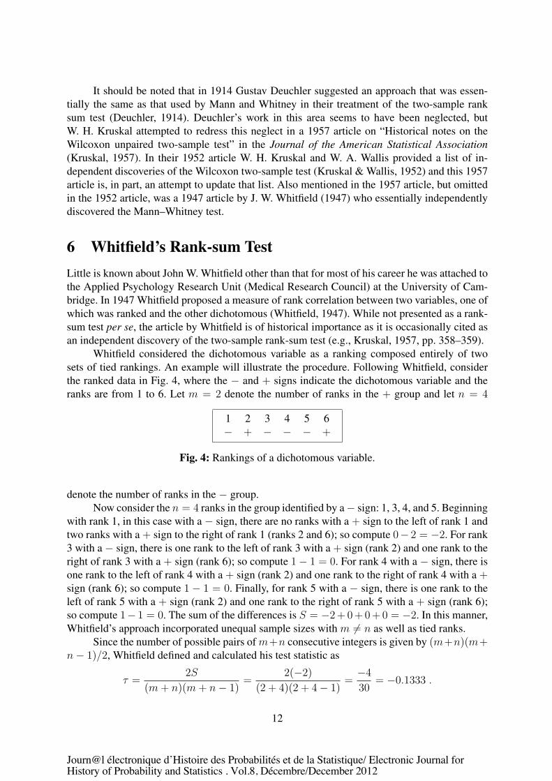
Whitfield considered the dichotomous variable as a ranking composed entirely of twosets of tied rankings. An example will illustrate the procedure. Following Whitfield, considerthe ranked data in Fig. 4, where the − and + signs indicate the dichotomous variable and theranks are from 1 to 6. Let m = 2 denote the number of ranks in the + group and let n = 4

1 2 3 4 5 6− + − − − +

Fig. 4: Rankings of a dichotomous variable.

denote the number of ranks in the − group.Now consider the n = 4 ranks in the group identified by a − sign: 1, 3, 4, and 5. Beginning

with rank 1, in this case with a − sign, there are no ranks with a + sign to the left of rank 1 andtwo ranks with a + sign to the right of rank 1 (ranks 2 and 6); so compute 0− 2 = −2. For rank3 with a − sign, there is one rank to the left of rank 3 with a + sign (rank 2) and one rank to theright of rank 3 with a + sign (rank 6); so compute 1− 1 = 0. For rank 4 with a − sign, there isone rank to the left of rank 4 with a + sign (rank 2) and one rank to the right of rank 4 with a +sign (rank 6); so compute 1 − 1 = 0. Finally, for rank 5 with a − sign, there is one rank to theleft of rank 5 with a + sign (rank 2) and one rank to the right of rank 5 with a + sign (rank 6);so compute 1− 1 = 0. The sum of the differences is S = −2+0+0+0 = −2. In this manner,Whitfield’s approach incorporated unequal sample sizes with m �= n as well as tied ranks.

Since the number of possible pairs of m+n consecutive integers is given by (m+n)(m+n− 1)/2, Whitfield defined and calculated his test statistic as

τ =2S

(m+ n)(m+ n− 1)=

2(−2)

(2 + 4)(2 + 4− 1)=

−4

30= −0.1333 .

12


It should be noted that in 1914 Gustav Deuchler suggested an approach that was essen-tially the same as that used by Mann and Whitney in their treatment of the two-sample ranksum test (Deuchler, 1914). Deuchler’s work in this area seems to have been neglected, butW. H. Kruskal attempted to redress this neglect in a 1957 article on “Historical notes on theWilcoxon unpaired two-sample test” in the Journal of the American Statistical Association(Kruskal, 1957). In their 1952 article W. H. Kruskal and W. A. Wallis provided a list of in-dependent discoveries of the Wilcoxon two-sample test (Kruskal & Wallis, 1952) and this 1957article is, in part, an attempt to update that list. Also mentioned in the 1957 article, but omittedin the 1952 article, was a 1947 article by J. W. Whitfield (1947) who essentially independentlydiscovered the Mann–Whitney test.

6 Whitfield’s Rank-sum TestLittle is known about John W. Whitfield other than that for most of his career he was attached tothe Applied Psychology Research Unit (Medical Research Council) at the University of Cam-bridge. In 1947 Whitfield proposed a measure of rank correlation between two variables, one ofwhich was ranked and the other dichotomous (Whitfield, 1947). While not presented as a rank-sum test per se, the article by Whitfield is of historical importance as it is occasionally cited asan independent discovery of the two-sample rank-sum test (e.g., Kruskal, 1957, pp. 358–359).

Whitfield considered the dichotomous variable as a ranking composed entirely of twosets of tied rankings. An example will illustrate the procedure. Following Whitfield, considerthe ranked data in Fig. 4, where the − and + signs indicate the dichotomous variable and theranks are from 1 to 6. Let m = 2 denote the number of ranks in the + group and let n = 4

1 2 3 4 5 6− + − − − +

Fig. 4: Rankings of a dichotomous variable.

denote the number of ranks in the − group.Now consider the n = 4 ranks in the group identified by a − sign: 1, 3, 4, and 5. Beginning

with rank 1, in this case with a − sign, there are no ranks with a + sign to the left of rank 1 andtwo ranks with a + sign to the right of rank 1 (ranks 2 and 6); so compute 0− 2 = −2. For rank3 with a − sign, there is one rank to the left of rank 3 with a + sign (rank 2) and one rank to theright of rank 3 with a + sign (rank 6); so compute 1− 1 = 0. For rank 4 with a − sign, there isone rank to the left of rank 4 with a + sign (rank 2) and one rank to the right of rank 4 with a +sign (rank 6); so compute 1 − 1 = 0. Finally, for rank 5 with a − sign, there is one rank to theleft of rank 5 with a + sign (rank 2) and one rank to the right of rank 5 with a + sign (rank 6);so compute 1− 1 = 0. The sum of the differences is S = −2+0+0+0 = −2. In this manner,Whitfield’s approach incorporated unequal sample sizes with m �= n as well as tied ranks.

Since the number of possible pairs of m+n consecutive integers is given by (m+n)(m+n− 1)/2, Whitfield defined and calculated his test statistic as

τ =2S

(m+ n)(m+ n− 1)=

2(−2)

(2 + 4)(2 + 4− 1)=

−4

30= −0.1333 .

12

Whitfield’s S is directly related to the U statistic of Mann and Whitney (1947) and, hence, to theW statistic of Wilcoxon (1945).6 Compare statistic S with the U statistic of Mann and Whitney.There are m = 2 + signs and n = 4 − signs in Fig. 4, so considering the lesser of the two (them = 2 + signs), the first + sign (rank 2) precedes three − signs (ranks 3, 4, and 5) and thesecond + sign precedes no − signs, so U = 3+0 = 3. The relationship between Whitfields’s Sand Mann and Whitney’s U is given by S = 2U −mn (Jonckheere, 1954; Kruskal, 1957); thus,S = 2(3)− (2)(4) = 6− 8 = −2. For the example data in Fig. 4, the Wilcoxon test statistic forthe smaller of the two sums (with the m = 2 + signs) is W = 2 + 6 = 8 and the relationshipwith S is given by S = m(m+n+1)− 2W ; thus, S = 2(2+4+1)− (2)(8) = 14− 16 = −2.

As Whitfield noted, the calculation of S was fashioned after a procedure first introducedby Kendall in 19457 and Whitfield was apparently unaware of the work by Wilcoxon, Festinger,and Mann and Whitney, as they are not referenced in the Whitfield article. Kendall (1945)considered the number of concordant (C) and discordant (D) pairs, of which there are a totalof (m + n)(m + n − 1)/2 pairs when there are no ties in the m + n consecutive integers. Forthe example data in Fig. 4 there are (2 + 4)(2 + 4 − 1)/2 = 15 pairs. Table 5 numbers andlists the 15 pairs, the concordant/discordant classification of pairs, and the pair values, whereconcordant pairs (−,− and +,+) are given a value of 0, and discordant pairs (+,− and −,+)are given values of +1 and −1, respectively. The sum of the pair values in Table 5 for the 15pairs is S = −5 + 3 = −2.

Today it is well known, although poorly documented, that when one classification is adichotomy and the other is ordered, with or without tied values, the S test of Kendall is equiva-lent to the Mann–Whitney U test (Burr, 1960; Moses, 1956). Whitfield was apparently the firstto discover the relationship between S, the statistic underlying Kendall’s τ correlation coeffi-cient, and U , the Mann–Whitney statistic for two independent samples. However, it was Jon-ckheere that was the first to make the relationship explicit (Jonckheere, 1954, p. 138). Becausethe Jonckheere–Terpstra test, when restricted to two independent samples, is mathematicallyidentical in reverse application to the Wilcoxon and Mann–Whitney tests (Leach, 1979, p. 183;Randles & Wolfe, 1979, p. 396), the two-sample rank-sum test is sometimes referred to as theKendall–Wilcoxon–Mann–Whitney–Jonckheere–Festinger test (Moses, 1956, p. 246).

Whitfield concluded his article with derivations of the variances of S for both untied andtied rankings and included a correction for continuity. For untied ranks the variance of S, asgiven by Kendall (1945), is σ2

S = {(m + n)(m + n − 1)[2(m + n) + 5]}/18 and the desiredprobability value is obtained from the asymptotically N(0, 1) distribution when min(m,n) →∞. For the example data listed in Fig. 4, the variance of S is σ2

S = {(2 + 4)(2 + 4 − 1)[2(2 +4) + 5]}/18 = 28.3333 and τ = S/σS = −2/

√28.3333 = −0.3757, with an approximate

lower one-sided probability value of 0.3536.An example will serve to illustrate the approach of Whitfield. It is common today to

transform a Pearson correlation coefficient between two variables (rxy) into Student’s pooled t

6Kraft and van Eeden show how Kendall’s τ can be computed as a sum of Wilcoxon W statistics (Kraft & vanEeden, 1968, pp. 180–181).

7Whitfield lists the date of the Kendall article as 1946, but the article was actually published in Biometrika in1945.

13


Table 5: Fifteen paired observations with concordant/discordant (C/D) pairs and associatedpair values.

Number Pair C/D Value Number Pair C/D Value1 1–2 −,+ −1 9 2–6 +,+ 02 1–3 −,− 0 10 3–4 −,− 03 1–4 −,− 0 11 3–5 −,− 04 1–5 −,− 0 12 3–6 −,+ −15 1–6 −,+ −1 13 4–5 −,− 06 2–3 +,− +1 14 4–6 −,+ −17 2–4 +,− +1 15 5–6 −,+ −18 2–5 +,− +1

test for two independent samples and vice-versa, i.e.,

t = rxy

√m+ n− 2

1− r2xyand rxy =

t√t2 +m+ n− 2

,

where m and n indicate the number of observations in Samples 1 and 2, respectively. It appearsthat Whitfield was the first to transform Kendall’s rank-order correlation coefficient τ into Mannand Whitney’s two-sample rank-sum statistic U for two independent samples. Actually, since

τ =2S

(m+ n)(m+ n− 1),

Whitfield established the relationship between the variable part of τ , Kendall’s S, and Mannand Whitney’s U . To illustrate just how Whitfield accomplished this, consider the data listed inFig. 5. The data consist of m = 12 adult ages from Sample A and n = 5 adult ages from SampleB, with associated ranks. The sample membership of the ages/ranks is indicated by an A or aB immediately beneath the rank score. Now, arrange the two samples into a contingency table

Age: 20 20 20 20 22 23 23 24 25 25 25 25 27 29 29 35 35

Rank: 212

212

212

212

5 612

612

9 1012

1012

1012

1012

13 1412

1412

1612

1612

Sample: A A A A B A A B A A A A B A A B B

Fig. 5: Listing of the m+ n = 17 raw age and rank scores from Samples A and B.

with two rows and columns equal to the frequency distribution of the combined samples, as inFig. 6. Here the first row of frequencies in Fig. 6 represents the runs in the list of ranks in Fig. 5labeled as A, i.e., there are four values of 21

2, no value of 5, two values of 61

2, no value of 9, four

values of 1012, and so on. The second row of frequencies in Fig. 6 represents the runs in the list

of ranks in Fig. 5 labeled as B, i.e., there is no value of 212

labeled as B, one value of 5, no value

14


Table 5: Fifteen paired observations with concordant/discordant (C/D) pairs and associatedpair values.

Number Pair C/D Value Number Pair C/D Value1 1–2 −,+ −1 9 2–6 +,+ 02 1–3 −,− 0 10 3–4 −,− 03 1–4 −,− 0 11 3–5 −,− 04 1–5 −,− 0 12 3–6 −,+ −15 1–6 −,+ −1 13 4–5 −,− 06 2–3 +,− +1 14 4–6 −,+ −17 2–4 +,− +1 15 5–6 −,+ −18 2–5 +,− +1

test for two independent samples and vice-versa, i.e.,

t = rxy

√m+ n− 2

1− r2xyand rxy =

t√t2 +m+ n− 2

,

where m and n indicate the number of observations in Samples 1 and 2, respectively. It appearsthat Whitfield was the first to transform Kendall’s rank-order correlation coefficient τ into Mannand Whitney’s two-sample rank-sum statistic U for two independent samples. Actually, since

τ =2S

(m+ n)(m+ n− 1),

Whitfield established the relationship between the variable part of τ , Kendall’s S, and Mannand Whitney’s U . To illustrate just how Whitfield accomplished this, consider the data listed inFig. 5. The data consist of m = 12 adult ages from Sample A and n = 5 adult ages from SampleB, with associated ranks. The sample membership of the ages/ranks is indicated by an A or aB immediately beneath the rank score. Now, arrange the two samples into a contingency table

Age: 20 20 20 20 22 23 23 24 25 25 25 25 27 29 29 35 35

Rank: 212

212

212

212

5 612

612

9 1012

1012

1012

1012

13 1412

1412

1612

1612

Sample: A A A A B A A B A A A A B A A B B

Fig. 5: Listing of the m+ n = 17 raw age and rank scores from Samples A and B.

with two rows and columns equal to the frequency distribution of the combined samples, as inFig. 6. Here the first row of frequencies in Fig. 6 represents the runs in the list of ranks in Fig. 5labeled as A, i.e., there are four values of 21

2, no value of 5, two values of 61

2, no value of 9, four

values of 1012, and so on. The second row of frequencies in Fig. 6 represents the runs in the list

of ranks in Fig. 5 labeled as B, i.e., there is no value of 212

labeled as B, one value of 5, no value

14

of 612, one value of 9, and so on. Finally, the column marginal totals are simply the sums of

the two rows. This contingency arrangement permitted Whitfield to transform a problem of thedifference between two independent samples into a problem of correlation between two rankedvariables.

A 4 0 2 0 4 0 2 0 12B 0 1 0 1 0 1 0 2 5

4 1 2 1 4 1 2 2 17

Fig. 6: Contingency table of the frequency of ranks in Fig. 5.

Denote by X the r × c table in Fig. 6 with r = 2 and c = 8 and let xij indicate a cellfrequency for i = 1, . . . , r and j = 1, . . . , c. Then, S can be expressed as the algebraic sum ofall second-order determinants in X (Burr, 1960):

S =r−1∑i=1

r∑j=i+1

c−1∑k=1

c∑l=k+1

(xikxjl − xilxjk) .

Thus, for the data listed in Fig. 6 there are c(c − 1)/2 = 8(8 − 1)/2 = 28 second-orderdeterminants:

S =

∣∣∣∣4 00 1

∣∣∣∣ +

∣∣∣∣4 20 0

∣∣∣∣ +

∣∣∣∣4 00 1

∣∣∣∣ +

∣∣∣∣4 40 0

∣∣∣∣ +

∣∣∣∣4 00 1

∣∣∣∣ +

∣∣∣∣4 20 0

∣∣∣∣ +

∣∣∣∣4 00 2

∣∣∣∣ + · · ·+∣∣∣∣2 00 2

∣∣∣∣ .

Therefore,

S = (4)(1)− (0)(0) + (4)(0)− (2)(0) + (4)(1)− (0)(0) + (4)(0)− (4)(0)

+ (4)(1)− (0)(0) + (4)(0)− (2)(0) + (4)(2)− (0)(0) + (0)(0)− (2)(1)

+ (0)(1)− (0)(1) + (0)(0)− (4)(1) + (0)(1)− (0)(1) + (0)(0)− (2)(1)

+ (0)(2)− (0)(1) + (2)(1)− (0)(0) + (2)(0)− (4)(0) + (2)(1)− (0)(0)

+ (2)(0)− (2)(0) + (2)(2)− (0)(0) + (0)(0)− (4)(1) + (0)(1)− (0)(1)

+ (0)(0)− (2)(1) + (0)(2)− (0)(1) + (4)(1)− (0)(0) + (4)(0)− (2)(0)

+ (4)(2)− (0)(0) + (0)(0)− (2)(1) + (0)(2)− (0)(1) + (2)(2)− (0)(0)

and S = 4 + 0 + 4 + · · ·+ 4 = 28.Alternatively, as Kendall (1948) has shown, the number of concordant pairs is given by

C =r−1∑i=1

c−1∑j=1

xij

(r∑

k=i+1

c∑l=j+1

xkl

)

and the number of discordant pairs is given by

D =r−1∑i=1

c−1∑j=1

xi,c−j+1

(r∑

k=i+1

c−j∑l=1

xkl

).

15


Thus for X in Fig. 6, C is calculated by proceeding from the upper-left cell with frequencyx11 = 4 downward and to the right, multiplying each cell frequency by the sum of all cellfrequencies below and to the right, and summing the products, i.e.,

C = (4)(1 + 0 + 1 + 0 + 1 + 0 + 2) + (0)(0 + 1 + 0 + 1 + 0 + 2)

+ (2)(1 + 0 + 1 + 0 + 2) + (0)(0 + 1 + 0 + 2)

+ (4)(1 + 0 + 2) + (0)(0 + 2) + (2)(2)

= 20 + 0 + 8 + 0 + 12 + 0 + 4 = 44 ,

and D is calculated by proceeding from the upper-right cell with frequency x18 = 0 downwardand to the left, multiplying each cell frequency by the sum of all cell frequencies below and tothe left, and summing the products, i.e.,

D = (0)(0 + 1 + 0 + 1 + 0 + 1 + 0) + (2)(1 + 0 + 1 + 0 + 1 + 0)

+ (0)(0 + 1 + 0 + 1 + 0) + (4)(1 + 0 + 1 + 0)

+ (0)(0 + 1 + 0) + (2)(1 + 0) + (0)(0)

= 0 + 6 + 0 + 8 + 0 + 2 + 0 = 16 .

Then, as defined by Kendall, S = C −D = 44− 16 = 28.To calculate Mann and Whitney’s U for the data listed in Fig. 5, the number of A ranks

to the left of (less than) the first B is 4; the number of A ranks to the left of the second B is6; the number of A ranks to the left of the third B is 10; and the number of A ranks to theleft of the fourth and fifth B are 12 each. Then U = 4 + 6 + 10 + 12 + 12 = 44. Finally,S = 2U −mn = (2)(44)− (12)(5) = 28. Thus Kendall’s S statistic, as redefined by Whitfield,includes as special cases Yule’s Q test for association in 2×2 contingency tables and the Mann–Whitney U test for larger contingency tables.

It is perhaps not surprising that Whitfield established a relationship between Kendall’s Sand Mann and Whitney’s U as Mann published a test for trend in 1945 that was identical toKendall’s S, as Mann noted (Mann, 1945). The Mann test is known today as the Mann–Kendalltest for trend where for n values in an ordered time series x1, . . . , xn,

S =n−1∑i=1

n∑j=i+1

sgn (xi − xj) ,

where

sgn(·) =

+1 if xi − xj > 0 ,

0 if xi − xj = 0 ,

−1 if xi − xj < 0 .

7 Haldane and Smith’s Rank-sum TestJohn Burton Sanderson Haldane was educated at Eton and New College, University of Oxford,and was a commissioned officer during World War I. At the conclusion of the war, Haldane was

16


Thus for X in Fig. 6, C is calculated by proceeding from the upper-left cell with frequencyx11 = 4 downward and to the right, multiplying each cell frequency by the sum of all cellfrequencies below and to the right, and summing the products, i.e.,

C = (4)(1 + 0 + 1 + 0 + 1 + 0 + 2) + (0)(0 + 1 + 0 + 1 + 0 + 2)

+ (2)(1 + 0 + 1 + 0 + 2) + (0)(0 + 1 + 0 + 2)

+ (4)(1 + 0 + 2) + (0)(0 + 2) + (2)(2)

= 20 + 0 + 8 + 0 + 12 + 0 + 4 = 44 ,

and D is calculated by proceeding from the upper-right cell with frequency x18 = 0 downwardand to the left, multiplying each cell frequency by the sum of all cell frequencies below and tothe left, and summing the products, i.e.,

D = (0)(0 + 1 + 0 + 1 + 0 + 1 + 0) + (2)(1 + 0 + 1 + 0 + 1 + 0)

+ (0)(0 + 1 + 0 + 1 + 0) + (4)(1 + 0 + 1 + 0)

+ (0)(0 + 1 + 0) + (2)(1 + 0) + (0)(0)

= 0 + 6 + 0 + 8 + 0 + 2 + 0 = 16 .

Then, as defined by Kendall, S = C −D = 44− 16 = 28.To calculate Mann and Whitney’s U for the data listed in Fig. 5, the number of A ranks

to the left of (less than) the first B is 4; the number of A ranks to the left of the second B is6; the number of A ranks to the left of the third B is 10; and the number of A ranks to theleft of the fourth and fifth B are 12 each. Then U = 4 + 6 + 10 + 12 + 12 = 44. Finally,S = 2U −mn = (2)(44)− (12)(5) = 28. Thus Kendall’s S statistic, as redefined by Whitfield,includes as special cases Yule’s Q test for association in 2×2 contingency tables and the Mann–Whitney U test for larger contingency tables.

It is perhaps not surprising that Whitfield established a relationship between Kendall’s Sand Mann and Whitney’s U as Mann published a test for trend in 1945 that was identical toKendall’s S, as Mann noted (Mann, 1945). The Mann test is known today as the Mann–Kendalltest for trend where for n values in an ordered time series x1, . . . , xn,

S =n−1∑i=1

n∑j=i+1

sgn (xi − xj) ,

where

sgn(·) =

+1 if xi − xj > 0 ,

0 if xi − xj = 0 ,

−1 if xi − xj < 0 .

7 Haldane and Smith’s Rank-sum TestJohn Burton Sanderson Haldane was educated at Eton and New College, University of Oxford,and was a commissioned officer during World War I. At the conclusion of the war, Haldane was

16

awarded a fellowship at New College, University of Oxford, and then accepted a readership inbiochemistry at Trinity College, University of Cambridge. In 1932 Haldane was elected a Fel-low of the Royal Society and a year later, became Professor of Genetics at University College,London. In 1956, Haldane immigrated to India where he joined the Indian Statistical Instituteat the invitation of P. C. Mahalanobis. In 1961 he resigned from the Indian Statistical Instituteand accepted a position as Director of the Genetics and Biometry Laboratory in Orissa, India.Haldane wrote 24 books, including science fiction and stories for children, more than 400 sci-entific research papers, and innumerable popular articles (Mahanti, 2007). Haldane died on 1December 1964, whereupon he donated his body to Rangaraya Medical College, Kakinada.

Cedric Austen Bardell Smith attended University College, London. In 1935, Smith re-ceived a scholarship to Trinity College, Unniversity of Cambridge, where he earned his Ph.D.in 1942. In 1946 Smith was appointed Assistant Lecturer at the Galton Laboratory, UniversityCollege, London, where he met J. B. S. Haldane. In 1964 Smith accepted an appointment asthe Weldon Professor of Biometry at University College, London. Cedric Smith clearly hada sense of humor and was known to occasionally sign his correspondence as “U. R. BlancheDescartes, Limit’d,” which was an anagram of Cedric Austen Bardell Smith (Morton, 2002).Over his career, Smith contributed to many of the classical topics in statistical genetics, includ-ing segregation ratios in family data, kinship, population structure, assortative mating, geneticcorrelation, and estimation of gene frequencies (Morton, 2002).8 Smith died on 10 January2002, just a few weeks shy of his 85th birthday (Edwards, 2002; Morton, 2002).

In 1948 Haldane and Smith introduced an exact test for birth-order effects (Haldane &Smith, 1948). They had previously observed that in a number of hereditary diseases and ab-normalities, the probability that any particular member of a sibship had a specified abnormalitydepended in part on his or her birth-rank (Haldane & Smith, 1948, p. 117). Specifically, theyproposed to develop a quick and simple test of significance of the effect of birth-rank based onthe sum of birth ranks of all affected cases in all sibships. In a classic description of a permu-tation test, Haldane and Smith noted that if in each sibship the numbers of normal and affectedsiblings were held constant, then if birth-rank had no effect, every possible order of normal andaffected siblings would be equally probable. Accordingly, the sum of birth-ranks for affectedsiblings would have a definite distribution, free from unknown parameters, providing “a ‘condi-tional’ and ‘exact’ test for effect of birth-rank” (Haldane & Smith, 1948, p. 117). Finally, theyobserved that this distribution would be very nearly normal in any practically occurring casewith a mean and variance that were easily calculable.

Consider a single sibship of k births, h of which are affected.9 Let the birth-ranks of theaffected siblings be denoted by a1, a2, . . . , ah and their sum by A =

∑hr=1 ar. Then, there are

(k

h

)=

k!

h!(k − h)!

equally-likely ways of distributing the h affected siblings. Of these, the number of ways ofdistributing them, Ph, k(A), so that their birth-ranks sum to A is equal to the number of partitions

8Cedric Smith, Roland Brooks, Arthur Stone, and William Tutte met at Trinity College, University of Cam-bridge, and were known as the Trinity Four. Together they published mathematical papers under the pseudonymBlanche Descartes, much in the tradition of the putative Peter Ørno, John Rainwater, and Nicolas Bourbaki.

9Haldane and Smith used k for the number of births and h for the number of affected births, instead of themore conventional n and r, respectively.

17


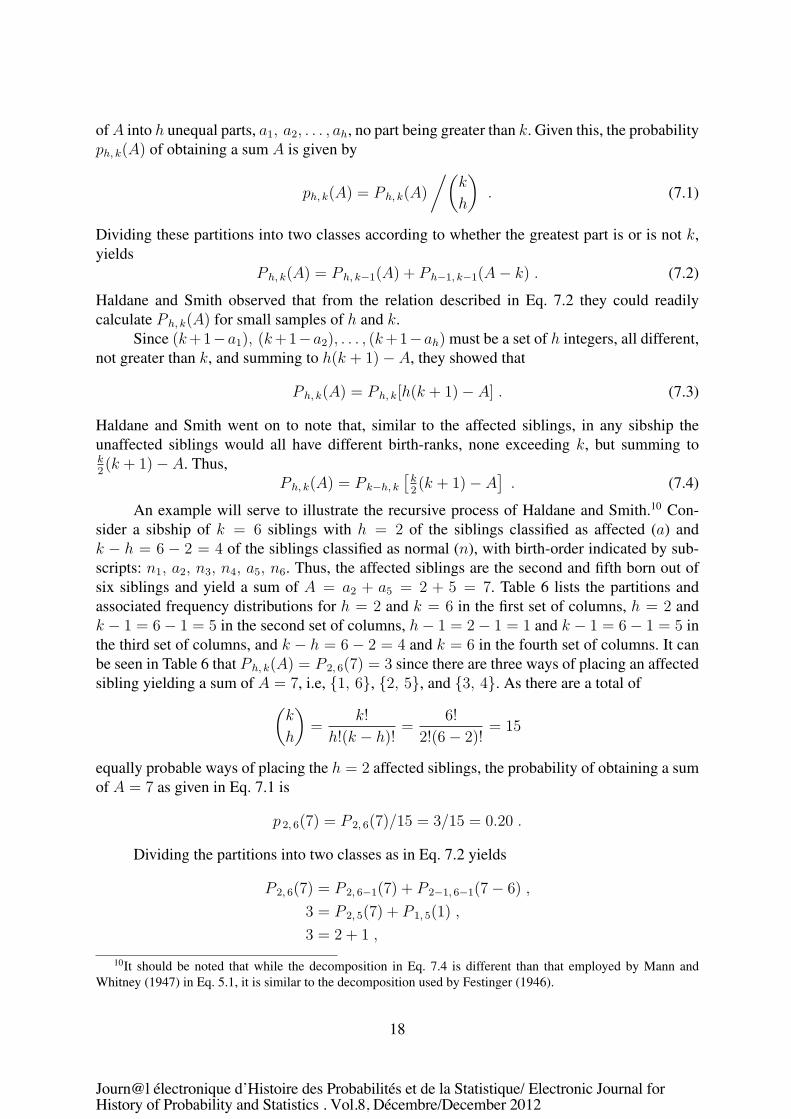
of A into h unequal parts, a1, a2, . . . , ah, no part being greater than k. Given this, the probabilityph, k(A) of obtaining a sum A is given by

ph, k(A) = Ph, k(A)

/(k

h

). (7.1)

Dividing these partitions into two classes according to whether the greatest part is or is not k,yields

Ph, k(A) = Ph, k−1(A) + Ph−1, k−1(A− k) . (7.2)

Haldane and Smith observed that from the relation described in Eq. 7.2 they could readilycalculate Ph, k(A) for small samples of h and k.

Since (k+1−a1), (k+1−a2), . . . , (k+1−ah) must be a set of h integers, all different,not greater than k, and summing to h(k + 1)− A, they showed that

Ph, k(A) = Ph, k[h(k + 1)− A] . (7.3)

Haldane and Smith went on to note that, similar to the affected siblings, in any sibship theunaffected siblings would all have different birth-ranks, none exceeding k, but summing tok2(k + 1)− A. Thus,

Ph, k(A) = P k−h, k

[k2(k + 1)− A

]. (7.4)

An example will serve to illustrate the recursive process of Haldane and Smith.10 Con-sider a sibship of k = 6 siblings with h = 2 of the siblings classified as affected (a) andk − h = 6 − 2 = 4 of the siblings classified as normal (n), with birth-order indicated by sub-scripts: n1, a2, n3, n4, a5, n6. Thus, the affected siblings are the second and fifth born out ofsix siblings and yield a sum of A = a2 + a5 = 2 + 5 = 7. Table 6 lists the partitions andassociated frequency distributions for h = 2 and k = 6 in the first set of columns, h = 2 andk − 1 = 6− 1 = 5 in the second set of columns, h− 1 = 2− 1 = 1 and k − 1 = 6− 1 = 5 inthe third set of columns, and k − h = 6− 2 = 4 and k = 6 in the fourth set of columns. It canbe seen in Table 6 that Ph, k(A) = P 2, 6(7) = 3 since there are three ways of placing an affectedsibling yielding a sum of A = 7, i.e, {1, 6}, {2, 5}, and {3, 4}. As there are a total of

(k

h

)=

k!

h!(k − h)!=

6!

2!(6− 2)!= 15

equally probable ways of placing the h = 2 affected siblings, the probability of obtaining a sumof A = 7 as given in Eq. 7.1 is

p 2, 6(7) = P 2, 6(7)/15 = 3/15 = 0.20 .

Dividing the partitions into two classes as in Eq. 7.2 yields

P 2, 6(7) = P 2, 6−1(7) + P 2−1, 6−1(7− 6) ,

3 = P 2, 5(7) + P 1, 5(1) ,

3 = 2 + 1 ,

10It should be noted that while the decomposition in Eq. 7.4 is different than that employed by Mann andWhitney (1947) in Eq. 5.1, it is similar to the decomposition used by Festinger (1946).

18


of A into h unequal parts, a1, a2, . . . , ah, no part being greater than k. Given this, the probabilityph, k(A) of obtaining a sum A is given by

ph, k(A) = Ph, k(A)

/(k

h

). (7.1)

Dividing these partitions into two classes according to whether the greatest part is or is not k,yields

Ph, k(A) = Ph, k−1(A) + Ph−1, k−1(A− k) . (7.2)

Haldane and Smith observed that from the relation described in Eq. 7.2 they could readilycalculate Ph, k(A) for small samples of h and k.

Since (k+1−a1), (k+1−a2), . . . , (k+1−ah) must be a set of h integers, all different,not greater than k, and summing to h(k + 1)− A, they showed that

Ph, k(A) = Ph, k[h(k + 1)− A] . (7.3)

Haldane and Smith went on to note that, similar to the affected siblings, in any sibship theunaffected siblings would all have different birth-ranks, none exceeding k, but summing tok2(k + 1)− A. Thus,

Ph, k(A) = P k−h, k

[k2(k + 1)− A

]. (7.4)

An example will serve to illustrate the recursive process of Haldane and Smith.10 Con-sider a sibship of k = 6 siblings with h = 2 of the siblings classified as affected (a) andk − h = 6 − 2 = 4 of the siblings classified as normal (n), with birth-order indicated by sub-scripts: n1, a2, n3, n4, a5, n6. Thus, the affected siblings are the second and fifth born out ofsix siblings and yield a sum of A = a2 + a5 = 2 + 5 = 7. Table 6 lists the partitions andassociated frequency distributions for h = 2 and k = 6 in the first set of columns, h = 2 andk − 1 = 6− 1 = 5 in the second set of columns, h− 1 = 2− 1 = 1 and k − 1 = 6− 1 = 5 inthe third set of columns, and k − h = 6− 2 = 4 and k = 6 in the fourth set of columns. It canbe seen in Table 6 that Ph, k(A) = P 2, 6(7) = 3 since there are three ways of placing an affectedsibling yielding a sum of A = 7, i.e, {1, 6}, {2, 5}, and {3, 4}. As there are a total of

(k

h

)=

k!

h!(k − h)!=

6!

2!(6− 2)!= 15

equally probable ways of placing the h = 2 affected siblings, the probability of obtaining a sumof A = 7 as given in Eq. 7.1 is

p 2, 6(7) = P 2, 6(7)/15 = 3/15 = 0.20 .

Dividing the partitions into two classes as in Eq. 7.2 yields

P 2, 6(7) = P 2, 6−1(7) + P 2−1, 6−1(7− 6) ,

3 = P 2, 5(7) + P 1, 5(1) ,

3 = 2 + 1 ,

10It should be noted that while the decomposition in Eq. 7.4 is different than that employed by Mann andWhitney (1947) in Eq. 5.1, it is similar to the decomposition used by Festinger (1946).

18

Table 6: Partitions (P ), sums (A), and frequencies (f ) for Ph, k(A) = P 2, 6(7), Ph, k−1(A) =P 2,5(7), Ph−1, k−1(A− k) = P 1, 5(1), and P k−h, k[

k2(k + 1)− A] = P 4,6(14).

P 2, 6(7) P 2, 5(7) P 1, 5(1) P4, 6(14)

P A f P A f P A f P A f

1, 2 3 1 1, 2 3 1 1 1 1 1, 2, 3, 4 10 11, 3 4 1 1, 3 4 1 2 2 1 1, 2, 3, 5 11 11, 4 5 2 1, 4 5 2 3 3 1 1, 2, 3, 6 12 21, 5 6 2 1, 5 6 2 4 4 1 1, 2, 4, 5 13 21, 6 7 3 2, 3 7 2 5 5 1 1, 2, 4, 6 14 32, 3 8 2 2, 4 8 1 1, 2, 5, 6 15 22, 4 9 2 2, 5 9 1 1, 3, 4, 5 16 22, 5 10 1 3, 4 1, 3, 4, 6 17 12, 6 11 1 3, 5 1, 3, 5, 6 18 13, 4 4, 5 1, 4, 5, 63, 5 2, 3, 4, 53, 6 2, 3, 4, 64, 5 2, 3, 5, 64, 6 2, 4, 5, 65, 6 3, 4, 5, 6

as illustrated in Table 6, where P2, 6(7) in the first set of columns is associated with a frequencyof 3, P 2,5(7) in the second set of columns is associated with a frequency of 2, and P1, 5(7−6) =P 1, 5(1) in the third set of columns is associated with a frequency of 1; thus, 3 + 2 + 1. Notethat once again, the decomposition observed in the discussion of Festinger and the two-samplerank sum test appears wherein

(k

h

)=

(k − 1

h

)+

(k − 1

h− 1

),

(6

2

)=

(6− 1

2

)+

(6− 1

2− 1

),

(6

2

)=

(5

2

)+

(5

1

),

15 = 10 + 5 .

This decomposition can be observed in Table 6, where the column of frequencies for P 2, 6(A)in the first set of columns sums to 15, the column of frequencies for P 2, 5(A) in the second setof columns sums to 10, the column of frequencies for P 1,5(A − k) in the third set of columnssums to 5, and 15 = 10 + 5.

From Eqs. 7.3 and 7.4, Haldane and Smith were able to construct a table of values ofPh, k(A) and

(kh

), giving the exact distribution for all values of k up to and including 12, noting

that values not explicitly given in the table could readily be derived by the use of Eqs. 7.3

19


and 7.4. Additionally, Haldane and Smith investigated the approximate distribution of A. Theyfound it more efficient to test 6A instead of A and showed that the theoretical mean of 6A was3h(k+1) and the theoretical variance was 3h(k+1)(k−h), and thus provided a table of meansand variances for h = 1, . . . , 18 and k = 2, . . . , 20. They observed that since A is made upof a number of independent components, the distribution of A would be approximately normaland, therefore, if an observed value of A exceeded the mean by more than twice the standarddeviation, siblings born later were most likely to be affected, but if the observed value of Afell short of the mean by the same amount, siblings born earlier were most likely to be affected(Haldane & Smith, 1948, p. 121). They concluded the paper with an example analysis based ondata from Munro on phenylketonuria from forty-seven British families (Munro, 1947).

8 van der Reyden’s Rank-sum TestLittle is known about D. van der Reyden other than that he was a statistician for the TobaccoResearch Board of Southern Rhodesia.11 In 1952 van der Reyden independently developed atwo-sample rank-sum test equivalent to the tests of Wilcoxon (1945), Festinger (1946), Mannand Whitney (1947), Whitfield (1947), and Haldane and Smith (1948), although none of these isreferenced; in fact, the article by van der Reyden contains no references whatsoever. The statedpurpose of the proposed test was to provide a simple exact test of significance using sums ofranks in order to avoid computing sums of squares (van der Reyden, 1952, p. 96). In a novelapproach, van der Reyden utilized a tabular format involving rotations of triangular matrices togenerate permutation distribution frequencies and published tables for tests of significance atthe 0.05, 0.02, and 0.01 levels (van der Reyden, 1952).

Table 7 illustrates the van der Reyden tabular procedure with values of n = 1, 2, 3,m = 1, . . . , 6, and sums of frequencies from T = 1 to T = 15. Looking first at the columnheaded n = 1 in Table 7, note that when m = 1 and n = 1, T = 1; when m = 2 and n = 1,T = 1 or 2; when m = 3 and n = 1, T = 1, 2, or 3; and when m = 4 and n = 1, T = 1,2, 3, or 4. Simply put, taking all samples of one item from m items, all values of T will havea frequency of 1. In this case, each T has a frequency of 1 and each frequency sums to

(mn

),

e.g., for m = 4 and n = 1 the frequency distribution is {1, 1, 1, 1} with a sum of 4, which is(41

)= 4. To obtain the frequencies for samples of n = 2 items, rotate all frequencies for n = 1

clockwise through 45◦, shifting the whole distribution downward to

T =

(n+ 1

2

)=

n(n+ 1)

2.

Thus in Table 7, the frequencies obtained for n = 1 are transposed with the first row nowconstituting the fourth column, the second row constituting the third column, and so on. Thenthis transposed matrix is shifted downward so it begins at T = n(n + 1)/2 = 2(2 + 1)/2 = 3.Finally, the frequencies are added together horizontally in the same manner as Festinger (1946),as follows.

Consider the frequency distributions listed under n = 2 in Table 7. There are two setsof frequency distributions under n = 2, one on the left and one on the right, both labeled

11Southern Rhodesia was shortened to Rhodesia in 1965 and renamed the Republic of Zimbabwe in 1980.

20


and 7.4. Additionally, Haldane and Smith investigated the approximate distribution of A. Theyfound it more efficient to test 6A instead of A and showed that the theoretical mean of 6A was3h(k+1) and the theoretical variance was 3h(k+1)(k−h), and thus provided a table of meansand variances for h = 1, . . . , 18 and k = 2, . . . , 20. They observed that since A is made upof a number of independent components, the distribution of A would be approximately normaland, therefore, if an observed value of A exceeded the mean by more than twice the standarddeviation, siblings born later were most likely to be affected, but if the observed value of Afell short of the mean by the same amount, siblings born earlier were most likely to be affected(Haldane & Smith, 1948, p. 121). They concluded the paper with an example analysis based ondata from Munro on phenylketonuria from forty-seven British families (Munro, 1947).

8 van der Reyden’s Rank-sum TestLittle is known about D. van der Reyden other than that he was a statistician for the TobaccoResearch Board of Southern Rhodesia.11 In 1952 van der Reyden independently developed atwo-sample rank-sum test equivalent to the tests of Wilcoxon (1945), Festinger (1946), Mannand Whitney (1947), Whitfield (1947), and Haldane and Smith (1948), although none of these isreferenced; in fact, the article by van der Reyden contains no references whatsoever. The statedpurpose of the proposed test was to provide a simple exact test of significance using sums ofranks in order to avoid computing sums of squares (van der Reyden, 1952, p. 96). In a novelapproach, van der Reyden utilized a tabular format involving rotations of triangular matrices togenerate permutation distribution frequencies and published tables for tests of significance atthe 0.05, 0.02, and 0.01 levels (van der Reyden, 1952).

Table 7 illustrates the van der Reyden tabular procedure with values of n = 1, 2, 3,m = 1, . . . , 6, and sums of frequencies from T = 1 to T = 15. Looking first at the columnheaded n = 1 in Table 7, note that when m = 1 and n = 1, T = 1; when m = 2 and n = 1,T = 1 or 2; when m = 3 and n = 1, T = 1, 2, or 3; and when m = 4 and n = 1, T = 1,2, 3, or 4. Simply put, taking all samples of one item from m items, all values of T will havea frequency of 1. In this case, each T has a frequency of 1 and each frequency sums to

(mn

),

e.g., for m = 4 and n = 1 the frequency distribution is {1, 1, 1, 1} with a sum of 4, which is(41

)= 4. To obtain the frequencies for samples of n = 2 items, rotate all frequencies for n = 1

clockwise through 45◦, shifting the whole distribution downward to

T =

(n+ 1

2

)=

n(n+ 1)

2.

Thus in Table 7, the frequencies obtained for n = 1 are transposed with the first row nowconstituting the fourth column, the second row constituting the third column, and so on. Thenthis transposed matrix is shifted downward so it begins at T = n(n + 1)/2 = 2(2 + 1)/2 = 3.Finally, the frequencies are added together horizontally in the same manner as Festinger (1946),as follows.

Consider the frequency distributions listed under n = 2 in Table 7. There are two setsof frequency distributions under n = 2, one on the left and one on the right, both labeled

11Southern Rhodesia was shortened to Rhodesia in 1965 and renamed the Republic of Zimbabwe in 1980.

20

Table 7: Generation of frequency arrays for n = 1, n = 2, and n = 3 as described by van derReyden.

n = 1 n = 2 n = 3

T/m 1 2 3 4 2 3 4 5 2 3 4 5 3 4 5 6 3 4 5 61 1 1 1 12 1 1 13 1 1 1 1 1 1 14 1 1 1 1 15 1 1 1 2 26 1 1 1 2 1 1 1 1 17 1 1 1 2 1 1 1 18 1 1 1 1 1 2 29 1 1 1 1 1 1 2 3

10 2 1 2 311 1 2 1 312 1 2 1 313 2 214 1 115 1 1

m = 2, 3, 4, 5. So, for example, to create the frequency distribution listed under n = 2, m = 3on the right, add together the frequency distribution listed under n = 2, m = 2 on the right andthe frequency distribution under n = 2, m = 3 on the left. To create the frequency distributionlisted under n = 2, m = 4 on the right, add together the frequency distribution listed undern = 2, m = 3 on the right and the frequency distribution under n = 2, m = 4 on the left.To create the frequency distribution listed under n = 2, m = 5 on the right, add together thefrequency distribution listed under n = 2, m = 4 on the right and the frequency distributionunder n = 2, m = 5 on the left. The process continues in this manner, recursively generatingthe required frequency distributions.

For a final example, consider the frequency distributions listed under n = 3 in Table 7.Again there are two sets of frequency distributions, one on the left and one on the right. Thedistribution on the left is created by rotating the distribution created under n = 2 on the right,and shifting it downward so it begins at T = n(n + 1)/2 = 3(3 + 1)/2 = 6. To create thefrequency distribution listed under n = 3, m = 6 on the right, add together the frequencydistribution listed under n = 3, m = 5 on the right and the frequency distribution under n =3, m = 6 on the left. The frequency distributions of sums in Table 7 can be compared with thefrequency distributions of sums in Table 3 that were generated with Festinger’s method. In thisrecursive manner van der Reyden created tables for T from n = 2, . . . , 12 and m = 10, . . . , 30for the α = 0.05, 0.02, and 0.01 levels of significance.

21


9 Further DevelopmentsIt would be remiss not to mention a later contribution by S. Siegel and J. W. Tukey. In 1960Siegel and Tukey developed a non-parametric two-sample test based on differences in variabilitybetween the two unpaired samples, rather than the more conventional tests for differences inlocation (Siegel & Tukey, 1960). The Siegel–Tukey test was designed to replace parametric Ftests for differences in variances that depended heavily on normality, such as Bartlett’s F andHartley’s Fmax tests for homogeneity of variance (Bartlett, 1937; Hartley, 1950). Within thisarticle Siegel and Tukey provided tables of one- and two-sided critical values based on exactprobabilities for a number of levels of significance.

Let the two sample sizes be denoted by n and m with n ≤ m and assign ranks to then + m ordered observations with low ranks assigned to extreme observations and high ranksassigned to central observations. Since the sum of the ranks is fixed, Siegel and Tukey chose towork with the sum of ranks for the smaller of the two samples, represented by Rn. They alsoprovided a table with one- and two-sided critical values of Rn for n ≤ m ≤ 20 for variouslevels of α.

Siegel and Tukey noted that their choice of ranking procedure, with low ranks assignedto extreme observations and high ranks assigned to central observations, allowed the use of thesame tables as were used for the Wilcoxon two-sample rank-sum test for location. Thus, asthey explained, their new test “[might] be considered a Wilcoxon test for spread in unpairedsamples” (Siegel & Tukey, 1960, p. 432). Alternatively, as they noted, the Siegel–Tukey tableswere equally applicable to the Wilcoxon (1945), Festinger (1946), Mann–Whitney (1947), andWhite (1952) rank-sum procedures for relative location of two unpaired samples, and wereappropriate linear transformations of the tabled values presented by Auble (1953).

In addition, a number of tables of exact probability values and/or tests of significancewere explicitly constructed for the two-sample rank-sum test in succeeding years, all basedon either the Wilcoxon or the Mann–Whitney procedure. By 1947 Wilcoxon had already pub-lished extended probability tables for the Wilcoxon W statistic (Wilcoxon, 1947). In 1952 C.White utilized the “elementary methods” of Wilcoxon to develop tables for the Wilcoxon Wstatistic when the numbers of items in the two independent samples were not necessarily equal(White, 1952). In 1953 D. Auble published extended tables for the Mann–Whitney U statistic(Auble, 1953) and in 1955 E. Fix and J. L. Hodges published extended tables for the WilcoxonW statistic (Fix & Hodges, 1955). In 1963 J. E. Jacobson published extensive tables for theWilcoxon W statistic (Jacobson, 1963) and in 1964 R. C. Milton published an extended tablefor the Mann–Whitney U statistic (Milton, 1964).

There were a number of errors in several of the published rank-sum tables that werecorrected in later articles; see especially the 1963 article by L. R. Verdooren (Verdooren, 1963)that contained corrections for the tables published by White (White, 1952) and Auble (Auble,1953), and an erratum to the 1952 article by Kruskal and Wallis (Kruskal & Wallis, 1952) thatcorrected errors in the tables published by White (White, 1952) and van der Reyden (van derReyden, 1952). By the mid-1960s tables of exact probability values were largely supplanted byefficient computer algorithms.

22


9 Further DevelopmentsIt would be remiss not to mention a later contribution by S. Siegel and J. W. Tukey. In 1960Siegel and Tukey developed a non-parametric two-sample test based on differences in variabilitybetween the two unpaired samples, rather than the more conventional tests for differences inlocation (Siegel & Tukey, 1960). The Siegel–Tukey test was designed to replace parametric Ftests for differences in variances that depended heavily on normality, such as Bartlett’s F andHartley’s Fmax tests for homogeneity of variance (Bartlett, 1937; Hartley, 1950). Within thisarticle Siegel and Tukey provided tables of one- and two-sided critical values based on exactprobabilities for a number of levels of significance.

Let the two sample sizes be denoted by n and m with n ≤ m and assign ranks to then + m ordered observations with low ranks assigned to extreme observations and high ranksassigned to central observations. Since the sum of the ranks is fixed, Siegel and Tukey chose towork with the sum of ranks for the smaller of the two samples, represented by Rn. They alsoprovided a table with one- and two-sided critical values of Rn for n ≤ m ≤ 20 for variouslevels of α.

Siegel and Tukey noted that their choice of ranking procedure, with low ranks assignedto extreme observations and high ranks assigned to central observations, allowed the use of thesame tables as were used for the Wilcoxon two-sample rank-sum test for location. Thus, asthey explained, their new test “[might] be considered a Wilcoxon test for spread in unpairedsamples” (Siegel & Tukey, 1960, p. 432). Alternatively, as they noted, the Siegel–Tukey tableswere equally applicable to the Wilcoxon (1945), Festinger (1946), Mann–Whitney (1947), andWhite (1952) rank-sum procedures for relative location of two unpaired samples, and wereappropriate linear transformations of the tabled values presented by Auble (1953).

In addition, a number of tables of exact probability values and/or tests of significancewere explicitly constructed for the two-sample rank-sum test in succeeding years, all basedon either the Wilcoxon or the Mann–Whitney procedure. By 1947 Wilcoxon had already pub-lished extended probability tables for the Wilcoxon W statistic (Wilcoxon, 1947). In 1952 C.White utilized the “elementary methods” of Wilcoxon to develop tables for the Wilcoxon Wstatistic when the numbers of items in the two independent samples were not necessarily equal(White, 1952). In 1953 D. Auble published extended tables for the Mann–Whitney U statistic(Auble, 1953) and in 1955 E. Fix and J. L. Hodges published extended tables for the WilcoxonW statistic (Fix & Hodges, 1955). In 1963 J. E. Jacobson published extensive tables for theWilcoxon W statistic (Jacobson, 1963) and in 1964 R. C. Milton published an extended tablefor the Mann–Whitney U statistic (Milton, 1964).

There were a number of errors in several of the published rank-sum tables that werecorrected in later articles; see especially the 1963 article by L. R. Verdooren (Verdooren, 1963)that contained corrections for the tables published by White (White, 1952) and Auble (Auble,1953), and an erratum to the 1952 article by Kruskal and Wallis (Kruskal & Wallis, 1952) thatcorrected errors in the tables published by White (White, 1952) and van der Reyden (van derReyden, 1952). By the mid-1960s tables of exact probability values were largely supplanted byefficient computer algorithms.

22

ReferencesAuble, D. (1953) Extended tables for the Mann–Whitney statistic, Bulletin of the Institute ofEducational Research, 1, 1–39.

Bartlett, M. S. (1937) Properties of sufficiency and statistical tests. Proceedings of the RoyalSociety of London, Series A (Mathematical and Physical Sciences), 160, 268–282.

Bradley, R. A. (1966) Frank Wilcoxon, Biometrics, 22, 192–194.

(1997) Frank Wilcoxon. In N. L. Johnson, and S. Kotz (eds.) Leading Personali-ties in Statistical Sciences: From the Seventeenth Century to the Present, Wiley: New York, pp.339–341.

and M. Hollander (2001) Wilcoxon, Frank. In C. C. Heyde and E. Seneta (eds.)Statisticians of the Centuries, Springer–Verlag: New York, pp. 420–424.

Burr, E. J. (1960) The distribution of Kendall’s score S for a pair of tied rankings. Biometrika,47, 151–171.

Deuchler, G. (1914) Uber die methoden der korrelationsrechnung in der padogogik und psy-chologie, Zeitschrift fur Padagogische Psychologie und Experimentelle Padagogik, 15, 114–131, 145–159, and 229–242.

Edwards, A. W. F. (2002) Professor C. A. B. Smith, 1917 – 2002, Journal of the Royal Statisti-cal Society, Series D (The Statistician), 51, 404–405.

Festinger, L. (1946) The significance of differences between means without reference to thefrequency distribution function, Psychometrika, 11, 97–105.

Fisher, R. A. (1925) Statistical Methods for Research Workers, Oliver and Boyd: Edinburgh.

Fix, E. and J. L. Hodges (1955) Significance probabilities of the Wilcoxon test, The Annals ofMathematical Statistics, 26, 301–312.

Friedman, M. (1937) The use of ranks to avoid the assumption of normality implicit in the anal-ysis of variance, Journal of the American Statistical Association, 32, 675–701.

Gini, C. (1916/1959) Il concetto di “Transvariazione” e le sue prime applicazioni, Giornaledegli economisti e Rivista di Statistica, 53, 13–43. Reproduced in Gini, C. (1959) Transvarizione.Memorie de Metodologia Statistica: Volume Secundo: a cura di Giuseppe Ottaviani, LibreriaGoliardia: Rome.

Haldane, J. B. S. and C. A. B. Smith (1948) A simple exact test for birth-order effect, Annals ofEugenics, 14, 117–124.

23


Hartley, H. O. (1950) The use of range in analysis of variance, Biometrika, 37, 271–280.

Hollander, M. (2000) A conversation with Ralph A. Bradley, Statistical Science, 16, 75–100.

Jacobson, J. E. (1963) The Wilcoxon two-sample statistic: Tables and bibliography, Journal ofthe American Statistical Association, 58, 1086–1103.

Jonckheere, A. R. (1954) A distribution-free k-sample test against ordered alternatives. Biometrika,41, 133–145.

Kendall, M. G. (1938) A New Measure of Rank Correlation, Biometrika, 30, 81–93.

(1945) The treatment of ties in ranking problems, Biometrika, 33, 239–251.

(1948) Rank Correlation Methods, Charles Griffin: London.

Kruskal, W. H. (1957) Historical notes on the Wilcoxon unpaired two-sample test, Journal ofthe American Statistical Association, 52, 356–360.

and W. A. Wallis (1952) Use of ranks in one-criterion variance analysis, Journalof the American Statistical Association, 47, 583–621. Erratum: Journal of the American Statis-tical Association, 48, 907–911 (1953).

Leach, C. (1979) Introduction to Statistics: A Nonparametric Approach for the Social Sciences,John Wiley & Sons: New York.

Lipmann, O. (1908) Eine methode zur vergleichung zwei kollektivgegenstanden, Zeitschrift furPsychologie, 48, 421–431.

MacMahon, P. A. (1916) Combinatory Analysis, Vol. II, Cambridge University Press: Cam-bridge.

Mahanti, S. (2007) John Burdon Sanderson Haldane: The ideal of a polymath, Vigyan PrasarScience Portal. Accessed on 20 January 2012 at http://www.vigyanprasar.gov.in/scientists/JBSHaldane.htm.

Mann, H. B. (1945) Nonparametric test against trend, Econometrica, 13, 245–259.

and D. R. Whitney (1947) On a test of whether one of two random variables isstochastically larger than the other, The Annals of Mathematical Statistics, 18, 50–60.

Milton, R. C. (1964) An extended table of critical values for the Mann–Whitney (Wilcoxon)two-sample dtatistic, Journal of the American Statistical Association, 59, 925–934.

24


Hartley, H. O. (1950) The use of range in analysis of variance, Biometrika, 37, 271–280.

Hollander, M. (2000) A conversation with Ralph A. Bradley, Statistical Science, 16, 75–100.

Jacobson, J. E. (1963) The Wilcoxon two-sample statistic: Tables and bibliography, Journal ofthe American Statistical Association, 58, 1086–1103.

Jonckheere, A. R. (1954) A distribution-free k-sample test against ordered alternatives. Biometrika,41, 133–145.

Kendall, M. G. (1938) A New Measure of Rank Correlation, Biometrika, 30, 81–93.

(1945) The treatment of ties in ranking problems, Biometrika, 33, 239–251.

(1948) Rank Correlation Methods, Charles Griffin: London.

Kruskal, W. H. (1957) Historical notes on the Wilcoxon unpaired two-sample test, Journal ofthe American Statistical Association, 52, 356–360.

and W. A. Wallis (1952) Use of ranks in one-criterion variance analysis, Journalof the American Statistical Association, 47, 583–621. Erratum: Journal of the American Statis-tical Association, 48, 907–911 (1953).

Leach, C. (1979) Introduction to Statistics: A Nonparametric Approach for the Social Sciences,John Wiley & Sons: New York.

Lipmann, O. (1908) Eine methode zur vergleichung zwei kollektivgegenstanden, Zeitschrift furPsychologie, 48, 421–431.

MacMahon, P. A. (1916) Combinatory Analysis, Vol. II, Cambridge University Press: Cam-bridge.

Mahanti, S. (2007) John Burdon Sanderson Haldane: The ideal of a polymath, Vigyan PrasarScience Portal. Accessed on 20 January 2012 at http://www.vigyanprasar.gov.in/scientists/JBSHaldane.htm.

Mann, H. B. (1945) Nonparametric test against trend, Econometrica, 13, 245–259.

and D. R. Whitney (1947) On a test of whether one of two random variables isstochastically larger than the other, The Annals of Mathematical Statistics, 18, 50–60.

Milton, R. C. (1964) An extended table of critical values for the Mann–Whitney (Wilcoxon)two-sample dtatistic, Journal of the American Statistical Association, 59, 925–934.

24

Morton, N. (2002) Cedric Smith (1917 – 2002), International Statistical Institute Newsletter,26, 9–10.

Moscovici, S. (1989) Obituary: Leon Festinger, European Journal of Social Psychology, 19,263–269.

Moses, L. E. (1956) Statistical theory and research design. Annual Review of Psychology, 7,233–258.

Munro, T. A. (1947) Phenylketonuria: Data on forty-seven British families, Annals of HumanGenetics, 14, 60–88.

Olson, J. (c. 2000) Henry Berthold Mann, Department of Mathematics, The Ohio State Univer-sity. Accessed on 20 January 2012 at http://www.math.osu.edu/history/biographies/mann.

Ottaviani, G. S. (1939) Probabilita che una prova su due variabili casuali X e Y verifichi ladisuguaglianza X < Y e sul Corrispondente Scarto Quadratico Medio, Giornale dell’IstitutoItaliano degli Attuari, 10, 186–192.

Pascal, B. (1665/1959) Traite du triangle arithmetique (Treatise on the arithmetical triangle). InD. E. Smith (ed.) A Source Book in Mathematics, Vol. 1, Dover, New York, pp. 67–79. Trans-lated by A. Savitsky.

Potvin, C. and D. A. Roff (1993) Distribution-free and robust statistical methods: Viable alter-natives to parametric statistics, Ecology, 74, 1615–1628.

Randles, R. H. and D. A. Wolfe (1979) Introduction to the Theory of Nonparametric Statistics,John Wiley & Sons: New York.

Siegel, S. and J. W. Tukey (1960) A nonparametric sum of ranks procedure for relative spreadin unpaired samples, Journal of the American Statistical Association, 55, 429–445.

Stigler, S. M. (1999) Statistics on the Table: The History of Statistical Concepts and Methods,Harvard University Press: Cambridge, MA.

van der Reyden, D. (1952) A simple statistical significance test, The Rhodesia AgriculturalJournal, 49, 96–104.

Vankeerberghen, P., C. Vandenbosh, J. Smeyers-Verbeke, and D. L. Massart (1991) Some robuststatistical procedures applied to the analysis of chemical data, Chemometrics and IntelligentLaboratory Systems, 12, 3–13.

Verdooren, L. R. (1963) Extended tables of critical values for Wilcoxon’s test statistic, Biometrika,50, 177–186.

25


White, C. (1952) The use of ranks in a test of significance for comparing two treatments, Bio-metrics, 8, 33–41.

Whitfield, J. W. (1947) Rank correlation between two variables, one of which is ranked, theother dichotomous, Biometrika, 34, 292–296.

Whitworth, W. A. (1942) Choice and Chance, New York: G. E. Stechert.

Wilcoxon, F. (1945) Individual comparisons by ranking methods, Biometrics Bulletin, 1, 80–83.

(1947) Probability tables for individual comparisons by ranking methods, Biomet-rics, 3, 119–122.

Willke, T. (2008) In Memoriam – Ransom Whitney, The Ohio State University, Departmentof Statistics News, 16. Accessed on 17 January 2012 at http://www.stat.osu.edu/sites/default/files/news/statnews2008.pdf.

26

The Two-sample Rank-sum Test: … journal articles attribute the origin of the two-sample rank-sum...

Documents

Transcript of The Two-sample Rank-sum Test: … journal articles attribute the origin of the two-sample rank-sum...