The Trend is the Cycle: Job Polarization and Jobless ... · The Trend is the Cycle: Job...

NBER WORKING PAPER SERIES

THE TREND IS THE CYCLE:JOB POLARIZATION AND JOBLESS RECOVERIES

Nir JaimovichHenry E. Siu

Working Paper 18334http://www.nber.org/papers/w18334

NATIONAL BUREAU OF ECONOMIC RESEARCH1050 Massachusetts Avenue

Cambridge, MA 02138August 2012

We thank David Andolfatto, Mark Aguiar, Susanto Basu, Paul Beaudry, Larry Christiano, MatiasCortes, Erik Hurst, Marianna Kudlyak, Ryan Michaels, Richard Rogerson, Aysegul Sahin, RobertShimer, Chris Taber, Marcelo Veracierto, Gianluca Violante, as well as numerous conference andseminar participants for helpful discussions. Domenico Ferraro provided expert research assistance.Siu thanks the Social Sciences and Humanities Research Council of Canada for support. The viewsexpressed herein are those of the authors and do not necessarily reflect the views of the National Bureauof Economic Research.

NBER working papers are circulated for discussion and comment purposes. They have not been peer-reviewed or been subject to the review by the NBER Board of Directors that accompanies officialNBER publications.

© 2012 by Nir Jaimovich and Henry E. Siu. All rights reserved. Short sections of text, not to exceedtwo paragraphs, may be quoted without explicit permission provided that full credit, including © notice,is given to the source.

The Trend is the Cycle: Job Polarization and Jobless RecoveriesNir Jaimovich and Henry E. SiuNBER Working Paper No. 18334August 2012, Revised March 2014JEL No. E0,J0

ABSTRACT

Job polarization refers to the recent shrinking concentration of employment in occupations in the middleof the skill distribution. Jobless recoveries refers to the slow rebound in aggregate employment followingrecent recessions, despite recoveries in aggregate output. We show how these two phenomena arerelated. First, essentially all employment loss in middle-skill occupations occurs in economic downturns;in this sense, job polarization has an important cyclical component. Second, jobless recoveries in theaggregate are accounted for by jobless recoveries in the middle-skill occupations that are disappearing.

Nir JaimovichDepartment of EconomicsDuke University213 Social Services BuildingDurham, NC 27708and [email protected]

Henry E. SiuDepartment of EconomicsUniversity of British Columbia1873 East Mall #997Vancouver, BC V6T 1Z1Canadaand [email protected]

1 Introduction

In the past 25 to 30 years, the US labor market has seen the emergence of two new phenomena:

job polarization and jobless recoveries. Job polarization refers to the increasing concentration

of employment in the highest- and lowest-wage occupations, as jobs in middle-skill occupations

disappear. Jobless recoveries refer to periods following recessions in which rebounds in aggregate

output are accompanied by much slower recoveries in aggregate employment. We argue that

these two phenomena are related.

Consider first the phenomenon of job polarization. Acemoglu (1999), Autor et al. (2006),

Goos and Manning (2007), and Goos et al. (2009) (among others) document that employment

is becoming concentrated at the tails of the occupational skill distribution. This process has

accelerated since the 1980s, as per capita employment in middle-skill jobs disappears. This

hollowing out of the middle is linked to the disappearance of occupations focused on “routine”

tasks—those activities that can be performed by following a well-defined set of procedures. Autor

et al. (2003) and the subsequent literature demonstrates that job polarization is due to “routine

biased technological change:” progress in technologies that substitute for labor in routine tasks.1

In this same time period, Gordon and Baily (1993), Groshen and Potter (2003), Bernanke

(2003), and Bernanke (2009) (among others) discuss the emergence of jobless recoveries. In the

past three recessions (of 1991, 2001, and 2009), aggregate employment continues to decline for

years following the turning point in aggregate income and output. No consensus has yet emerged

regarding the source of these jobless recoveries.

In this paper, we demonstrate that the two phenomena are related. We report two related

findings. First, the disappearance of per capita employment in routine occupations associated

with job polarization is not simply a gradual phenomenon: the loss is concentrated in economic

downturns. Specifically, 88% of the job loss in these occupations since the mid-1980s occurs

within a 12 month window of NBER dated recessions (that have all been characterized by

jobless recoveries). In this sense, the long-run or “trend” change in the skill distribution of

employment has an important business “cycle” component. A number of researchers have noted

that the polarization process has been accelerated by the Great Recession (see Autor (2010); and

Brynjolfsson and McAfee (2011)). Our first point is that routine employment loss has happened

almost entirely in the last three recessions.

Our second point is that job polarization accounts for jobless recoveries. This argument is

based on three facts. First, employment in the routine occupations identified by Autor et al.

(2003), Autor and Dorn (2012), and others account for a significant fraction of aggregate em-

ployment; averaged over the jobless recovery era, these jobs account for about 50% of total

1See also Firpo et al. (2011), Goos et al. (2011), and the references therein regarding the role of outsourcingand offshoring in job polarization.

2

employment. Second, essentially all of the contraction in per capita aggregate employment

during NBER dated recessions can be attributed to recessions in these middle-skill, routine oc-

cupations. Third, jobless recoveries are observed only in these disappearing, middle-skill jobs.

The high- and low-skill occupations to which employment is polarizing either do not experience

contractions, or if they do, rebound soon after the turning point in aggregate output. Hence, job-

less recoveries can be traced to the disappearance of routine occupations in recessions. Finally,

it is important to note that jobless recoveries were not observed in routine occupations—nor in

aggregate employment—prior to the era of job polarization.

In Section 2, we present data on jobless recoveries and job polarization. In Section 3, we

present data documenting our two principal findings, that these two phenomena are related. In

Section 4, we present a search-and-matching model of the labor market in which routine biased

technological change is a trend phenomenon. Nonetheless, middle-skill job loss is concentrated

in downturns, and recoveries from these events are jobless. Section 5 concludes.

2 Two Labor Market Phenomena

2.1 Jobless Recoveries

Figures 1 and 2 plot the cyclical behavior of aggregate per capita employment in the US during

the past six recessions and subsequent recoveries.2 Aggregate per capita employment is that

of all civilian non-institutionalized individuals aged 16 years and over (seasonally adjusted),

normalized by the population.3 Because the monthly employment data are “noisy,” the data

are logged and band pass filtered to remove only fluctuations at frequencies higher than 18

months (business cycle fluctuations are traditionally defined as those between frequencies of 18

and 96 months).4 On the x-axis of each figure, the trough of the recession, as identified by the

NBER, is indicated as date 0; we plot data for two years around the trough date. The shaded

regions indicate the NBER peak-to-trough periods. Employment is normalized to zero at the

trough of each recession. Hence, the y-axis measures the percent change in employment relative

2The 1980 recession is omitted since it is followed closely by a recession beginning in 1981, limiting our abilityto study its recovery. Throughout the paper, recessions are referred to by their trough year, e.g., the recessionthat began in December 2007 and ended in June 2009 is referred to as the 2009 recession.

3Data are taken from the Labor Force Statistics of the CPS, downloaded from the BLS website(http://www.bls.gov/data/). See Appendix A for detailed description of all data sources. Employment dataat the aggregate and occupational level are available dating back to 1959. However, there are well-documentedissues with the early CPS data, especially during the 1961 recession; see, for instance, the 1962 report of thePresident’s Committee to Appraise Employment and Unemployment Statistics entitled “Measuring Employmentand Unemployment.” The recommendations of this report (commonly referred to as the Gordon report) led tomethodological changes adopted by the BLS beginning in 1967 (see Stein (1967)). As such, our analysis uses databeginning in July 1967.

4We implement this using the band pass filter proposed by Christiano and Fitzgerald (2003), who discuss themerits of their method for isolating fluctuations outside the traditional business cycle frequencies and near theendpoints of datasets.

3

http://www.bls.gov/data/

Figure 1: Aggregate Employment around Early NBER Recessions

Notes: Data from the Bureau of Labor Statistics, Current Population Survey. See Appendix A for details.

4

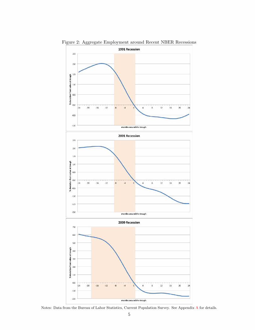
Figure 2: Aggregate Employment around Recent NBER Recessions


5

to its value in the NBER trough.

Figure 1 displays the 1970, 1975, and 1982 recessions. In each case, aggregate employment

begins to expand within six months of the trough. The fact that employment recovers within

two quarters of the recovery in aggregate output and income is typical of the business cycle prior

to the mid-1980s (see for instance, Schreft and Singh (2003); Groshen and Potter (2003)).

This contrasts sharply from the 1991, 2001, and 2009 recessions. As displayed in Figure 2,

these recoveries were jobless: despite expansions in other measures of economic activity (such as

RGDP and real gross domestic income) following the trough, aggregate per capita employment

continued to contract for many months. In 1991, employment continues to fall for 17 months

past the trough before turning around; employment does not reach its pre-recession level until

five years later, in 1996. In 2001, employment falls for 23 months past the trough before turning

around; it does not return to its pre-recession level before the subsequent recession. Following

the Great Recession of 2009, employment takes 23 months to begin recovery. Hence, the jobless

recovery is a phenomenon characterizing recent recessions (see also Groshen and Potter (2003)

and Bernanke (2003)).

Table 1 summarizes these differences, presenting several measures of the speed of recovery

following early and recent recessions. Panel A concerns the recoveries in aggregate per capita

employment. The first row lists the number of months it takes for employment to turn around

(stop contracting), relative to the NBER trough date. The second row indicates the number of

months it takes from the trough date for employment to return to its level at the trough. The

third row lists a “half-life” measure: the number of months it takes from the trough date to

regain half of the employment lost during the NBER-defined recession.

As is obvious, there has been a marked change in the speed of employment recoveries.

Averaged over the three early recessions, employment turns around approximately four months

after the NBER trough date; in the recent recessions, the average turnaround time is 21 months.

Averaged over the early recessions, employment returns to its trough level within approximately

10 months. In the 1991 and 2001 recessions, this takes 31 and 55 months, respectively; as of

December 2013, employment has yet to return to the trough level since the end of the 2009

recession. Finally, while it takes at most 27 months from the trough date to regain half of the

employment lost in the three early recessions, it takes at least 38 months in the recent recessions;

indeed, employment never regained half of its loss following the 2001 recession, and has yet to

do so after the Great Recession.

This contrasts with the nature of recoveries in aggregate output. Panel B presents the

same recovery measures for per capita RGDP; to obtain monthly measures, we use the monthly

data of Stock and Watson (see Appendix A for details). Given the NBER Dating Committee’s

emphasis on RGDP and real gross domestic income in determining cyclical turning points, it is

perhaps not surprising that aggregate output begins recovery on the NBER trough dates (see

6

Table 1: Measures of Recovery following Early and Recent Recessions

Early Recent

1970 1975 1982 1991 2001 2009

A. Employment

months to turn around 6 4 2 17 23 23

months to trough level 16 10 4 31 55 NA

half-life (in months) 27 23 10 38 NA NA

B. Output

months to turn around 0 0 0 0 0 0

months to trough level 0 0 0 0 0 0

half-life (in months) 7 10 5 9 3 15

Notes: Data from the Bureau of Labor Statistics, Current Population Survey; Bureau ofEconomic Analysis, National Income and Product Accounts; and James Stock and MarkWatson. See Appendix A for details.

http://www.nber.org/cycles/recessions faq.html). This is true for both the early and recent

recessions, as indicated by the first two rows of Panel B. In the early recessions, it takes on

average seven months from the trough date for output to regain half of its recessionary loss;

in the recent recessions, the average time taken is nine months, only slightly greater.5 Hence,

there has been no marked change in the speed of recovery for aggregate output across early

and recent recessions. The differences in the speed of recovery in employment following recent

recessions—without corresponding differences in the recovery speed of output—characterize the

jobless recovery phenomenon.

2.2 Job Polarization

The structure of employment has changed dramatically in the past 25 to 30 years. One of the

most pervasive aspects of change has been within the skill distribution: employment has become

polarized, with employment share shifting away from middle-skill occupations towards both the

high- and low-skill tails of the distribution (see, for instance, Acemoglu and Autor (2011), and

the references therein).

To see this, we disaggregate total employment by occupational groups. In Appendix A,

we discuss the occupational classification in detail; Appendix B discusses robustness of our

results to alternative classifications used in the literature. For brevity, we include a summary

5Because the monthly RGDP estimates of Stock and Watson are “noisy,” the data are band pass filtered toremove fluctuations at frequencies higher than 18 months (as with the employment data) in producing the half-lifestatistics.

7

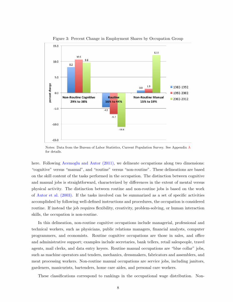
http://www.nber.org/cycles/recessions_faq.html

Figure 3: Percent Change in Employment Shares by Occupation Group

Notes: Data from the Bureau of Labor Statistics, Current Population Survey. See Appendix Afor details.

here. Following Acemoglu and Autor (2011), we delineate occupations along two dimensions:

“cognitive” versus “manual”, and “routine” versus “non-routine”. These delineations are based

on the skill content of the tasks performed in the occupation. The distinction between cognitive

and manual jobs is straightforward, characterized by differences in the extent of mental versus

physical activity. The distinction between routine and non-routine jobs is based on the work

of Autor et al. (2003). If the tasks involved can be summarized as a set of specific activities

accomplished by following well-defined instructions and procedures, the occupation is considered

routine. If instead the job requires flexibility, creativity, problem-solving, or human interaction

skills, the occupation is non-routine.

In this delineation, non-routine cognitive occupations include managerial, professional and

technical workers, such as physicians, public relations managers, financial analysts, computer

programmers, and economists. Routine cognitive occupations are those in sales, and office

and administrative support; examples include secretaries, bank tellers, retail salespeople, travel

agents, mail clerks, and data entry keyers. Routine manual occupations are “blue collar” jobs,

such as machine operators and tenders, mechanics, dressmakers, fabricators and assemblers, and

meat processing workers. Non-routine manual occupations are service jobs, including janitors,

gardeners, manicurists, bartenders, home care aides, and personal care workers.

These classifications correspond to rankings in the occupational wage distribution. Non-

8

routine cognitive occupations tend to be high-skill occupations and non-routine manual occu-

pations low-skilled. Routine occupations—both cognitive and manual—tend to be middle-skill

occupations (see, for instance, Autor (2010); and Firpo et al. (2011)). Given this, we combine

the routine cognitive and routine manual occupations into one group.6

Figure 3 displays data relating to job polarization. We present data by decade, as is common

in the literature (see, for instance, Autor (2010)). Each bar represents the percent change in an

occupation group’s share of total employment. Over time, the share of employment in high-skill

(non-routine cognitive) and low-skill (non-routine manual) jobs has been growing. This has

been accompanied by a hollowing out of the middle-skill, routine occupations. Hence, there

has been a polarization in employment away from routine, middle-skill jobs toward non-routine

cognitive and manual jobs. In 1982, routine occupations accounted for approximately 56% of

total employment; in 2012, this share has fallen to 44%.

3 Linking the Two Phenomena

3.1 Occupational Employment: The Bigger Picture

In this subsection, we ask how the process of job polarization has unfolded over time. In particu-

lar, has it occurred gradually, or is polarization “bunched up” within certain time intervals? To

investigate this, Figure 4 displays time series for per capita employment in the three occupational

groups at a monthly frequency from July 1967 to December 2013.

As is evident from the figure, both of the non-routine occupational groups are growing

over time. Per capita employment in non-routine cognitive occupations displays a 53 log point

increase during this period. After declining from 1967 to 1972, non-routine manual employment

displays a 19 log point increase. Recessions have temporarily halted these occupations’ growth

to varying extents, but have not abated the upward trends.

This stands in stark contrast to the routine occupational group. In per-capita terms, routine

employment was relatively constant until the late-1980s, and has fallen 29 log points from the

local peak in 1990 to present.

The trend growth of per capita employment in non-routine jobs (coupled with the lack of

growth in routine jobs) makes it clear that the share of employment in routine occupations has

been in decline since at least 1967. Hence, the job polarization era that began in the 1980s does

not simply represent a relative decline in routine employment, but the obvious acceleration of this

decline. This acceleration is due to the fact that per capita routine employment is disappearing

6For brevity, the analogs of all of our figures with the routine occupations split into two groups can be foundin an earlier version of this paper, available at http://faculty.arts.ubc.ca/hsiu/research/polar20120331.pdf. Noneof our substantive results are changed when considering the routine cognitive and manual occupations separately.

9

http://faculty.arts.ubc.ca/hsiu/research/polar20120331.pdf

Figure 4: Employment in Occupational Groups: 1967 – 2013


10

in absolute terms. As such, and given our interest in jobless recoveries in per capita aggregate

employment, we focus on the decline of per capita employment in routine occupations.

What is equally clear in Figure 4 is that routine job loss has not occurred steadily during the

past 25 or 30 years. The decline in routine occupations is concentrated in economic downturns.

This occurred in essentially three steps. Following its peak in 1990, per capita employment in

these occupations fell 3.5% to the trough of the 1991 recession, and a further 1.8% during the

subsequent jobless recovery. After a minor rebound, employment was essentially flat until the

2001 recession. In the two year window around the 2001 trough, this group shed 6.2% of its

employment, before leveling off again. Routine employment has plummeted again in the Great

Recession—11.3% in the two year window around the trough—with no subsequent recovery.

To state this slightly differently, 88% of the 29 log point fall in per capita routine employment

that occurred from 1990 to present occurred within a 12 month window of NBER recessions (six

months prior to the peak and six months after the trough). Hence, this stark element of job

polarization is observed during recessions; it is a business cycle phenomenon.

3.2 Occupational Employment: Business Cycle Snapshots

During the polarization period, per capita employment in routine occupations disappeared dur-

ing recessions. Moreover, as Figure 4 makes clear, prior to job polarization, routine employment

always recovered following recessions. In this subsection, we investigate whether job polariza-

tion has contributed to the jobless recoveries following the three most recent recessions. This is

quantitatively plausible since routine occupations account for a substantial fraction of aggregate

employment.

To do this, we “zoom in” on recessionary episodes; Figures 5 and 6 plot per capita em-

ployment for the routine and non-routine occupational groups around NBER recessions. These

figures are constructed in the same manner as Figures 1 and 2.7

Figure 5 displays the early recessions of 1970, 1975, and 1982 and their subsequent recoveries.

Contractions in employment are clearly observed in the routine occupations. In the non-routine

occupational group, employment was either flat or growing during these recessions and recoveries.

Hence, the contractions in per capita aggregate employment displayed in Figure 1, are due almost

exclusively to the routine occupations; this is true, despite the fact that routine occupations

account for only 58% of total employment, averaged over the 1967–1982 period. Measuring from

NBER peak to trough, 97% of all job loss in both the 1970 and 1975 recessions was accounted

for by job loss in routine occupations. In the 1982 recession, job loss in routine occupations

accounted for 145% of the aggregate, as employment actually grew in the non-routine group.

7For the analogous figures with the non-routine cognitive and non-routine manual groups displayed separately,see Appendix B.

11

Figure 5: Occupational Employment around Early NBER Recessions


12

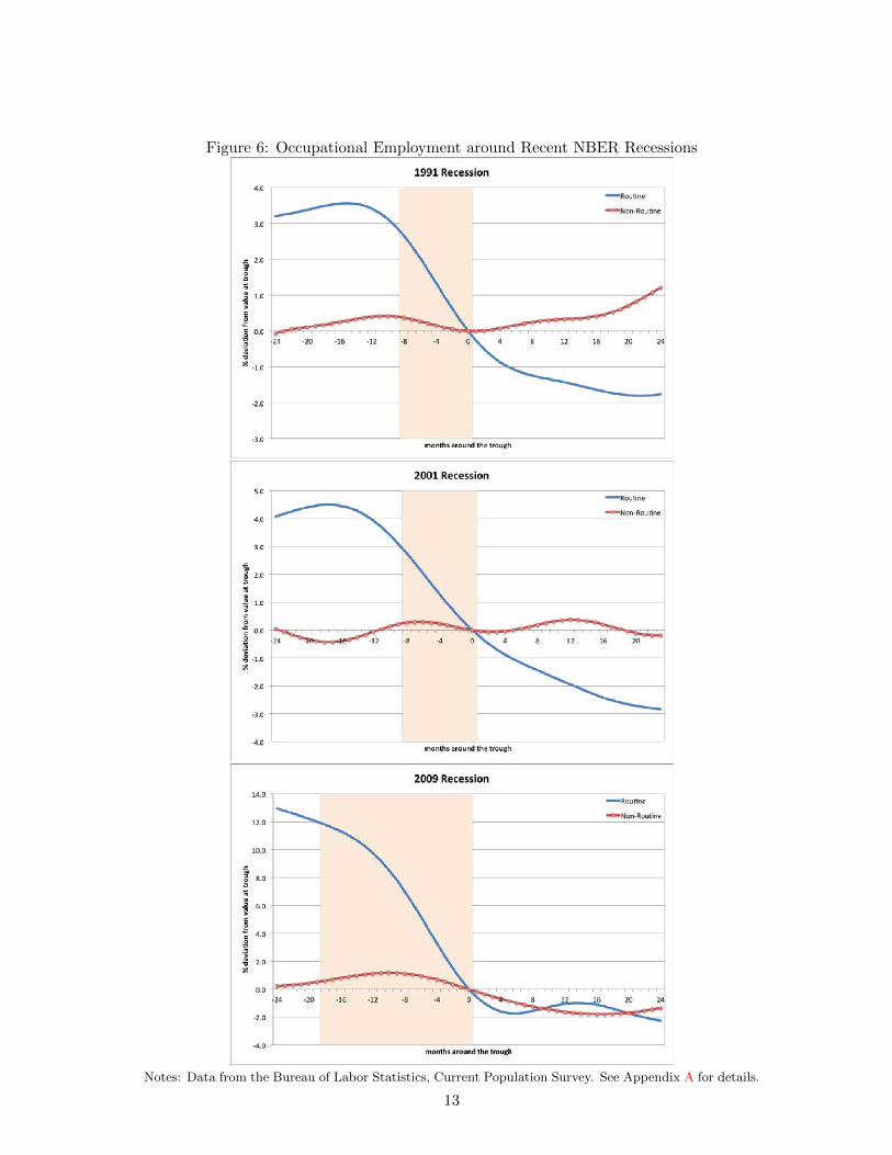
Figure 6: Occupational Employment around Recent NBER Recessions


13

Moreover, no jobless recoveries were observed in the routine occupational group. Following

these recessions, routine employment begins recovering within 7 months of the trough. This

mirrors the lack of jobless recoveries at the aggregate level displayed in Figure 1. Comparing

Figures 1 and 5, it is clear that the cyclical dynamics of aggregate employment in the 1970,

1975, and 1982 episodes are driven by the dynamics of routine employment.

Comparing Figures 2 and 6, it is again clear that the recession and recovery dynamics of

aggregate employment in 1991, 2001, and 2009 are driven by the dynamics of routine employ-

ment. Consider, for instance, the 1991 recession displayed in the uppermost panels. In the 15

months prior to the trough, per capita aggregate employment falls by 2.0%, and falls a further

0.5% during the 24 month window after the recession displayed in Figure 2. Figure 6 indicates

that this pattern is not exhibited in non-routine occupations. During this time window, per

capita non-routine employment rises, with only a mild (0.4%) contraction and clear recovery

beginning on the NBER trough date. Only routine employment exhibits the same pattern as in

the aggregate, with a 3.5% fall in the 15 months prior to the trough, and a further 1.8% decline

in the 24 month recovery period.

Indeed, Figure 6 indicates that routine occupations experience jobless recoveries in all three

episodes in the job polarization era. Per capita routine employment experience clear contractions

during each recession. As with the early episodes, these occupations account for the bulk of the

contraction in aggregate employment. In the 1991, 2001, and 2009 recessions, routine jobs

account for 89%, 91%, and 94% of all job loss, respectively. This is despite the fact that routine

occupations account for approximately 50% of total employment, averaged over 1983–2013.

More importantly, routine occupations show no recoveries in Figure 6. As discussed above,

employment in routine occupations falls a further 1.8% in the 24 months following the end of the

1991 recession. A similar picture emerges for the 2001 recession: large employment losses leading

up to the trough are followed by a further 2.8% loss afterward. In 2009, these occupations are

hit especially hard, falling 11.8% from the NBER peak to trough, and a further 2.3% in the two

years after. Indeed, per capita routine employment shows no recovery to date, down 3.5% from

the recession’s trough to December 2013.

To summarize, jobless recoveries are evident in only the three most recent recessions and

are only clearly evident in routine occupations. In this occupational group, employment never

recovers—in the short-, medium- or long-term. These occupations are disappearing. By contrast,

non-routine occupations either experience no contractions or only mild contractions in recessions,

and no jobless recoveries afterwards. In this sense, the jobless recovery phenomenon is due to

the disappearance of routine jobs.

14

3.3 A Counterfactual Experiment

To make this final point clear, we perform a simple accounting experiment to investigate, at a

first pass, the role of job polarization—specifically, the disappearance of routine employment—in

accounting for jobless recoveries. This is an informative exercise since recessions in aggregate

employment are due almost entirely to recessions in routine occupations, as discussed above. We

ask what would have happened in recent recessions if the post-recession behavior of employment

in routine occupations had looked more similar to the early recessions. Would the economy still

have experienced jobless recoveries in the aggregate?8

For the 1991, 2001, and 2009 recessions, we replace the per capita employment in routine

occupations following the trough with their average response following the troughs of the 1970,

1975, and 1982 recessions. We do this in a way that matches the magnitude of the fall in

employment after each recent recession, but follows the time pattern of the early recessions.

In particular, we ensure that the turning point in routine employment comes 5 months after

the trough, as in the average of those recoveries. We then sum up the actual employment in

non-routine occupations with the counterfactual employment in routine occupations to obtain a

counterfactual aggregate employment series. The behavior of these counterfactual series around

the recent NBER trough dates is displayed in Figure 7. Further details regarding the construction

of the counterfactuals is discussed in Appendix C.

Figure 7 makes clear that had it not been for the disappearance of routine jobs that occurs

during recessions, we would not have observed jobless recoveries. Aggregate employment would

have experienced clear turning points 5, 5, and 7 months after the troughs of the 1991, 2001, and

2009 recessions, respectively. In the 1991 and 2001 recessions, employment would have exceeded

its value at the NBER-dated trough within 10 months. In the case of the 2009 recession, recovery

back to the trough level would have taken 18 months. This is due to the fact that the recent, and

far more severe, Great Recession was experienced more broadly across occupations, and because

routine employment represents a shrinking share of total employment over time.9 Nonetheless,

employment would have recovered, as opposed to declining in the 24 months following the end

of the recession.

Finally, we note again that jobless recoveries cannot be accounted for by a change in the

post-recession behavior of employment in non-routine occupations. This is, perhaps, not surpris-

ing given that the dynamics of non-routine employment play little role in the that of aggregate

8In spite of the results presented in subsection 3.2, we note that the answer to this is not immediate since,in the jobless recovery period, routine jobs account for only 50% of aggregate employment. Reversing joblessrecoveries in routine employment may not be quantitatively important enough to reverse them in the aggregate.

9Interestingly, while employment in non-routine occupations suffered only mild contraction during the recession(falling 1.1% in the ten months prior to the trough), it continued to contract by 1.8% in the sixteen monthsfollowing the NBER trough date. Hence, and perhaps not surprisingly, the malaise in the labor market followingthe 2009 recession is not solely accounted for by routine occupations.

15

Figure 7: Actual and Counterfactual Employment around Recent NBER Recessions

Notes: Actual data from the Bureau of Labor Statistics, Current Population Survey; counterfactualsdescribed in Appendix C.

16

employment during recessions, as discussed in subsection 3.2. Nonetheless, we have performed

the same counterfactual as above, but replacing the employment response in non-routine occu-

pations following the recent recessions with their average response following the early recessions.

Though not displayed here for brevity, we find that this generates no clear recovery in aggre-

gate employment beyond its trough value in any of the recent episodes. By contrast, aggregate

employment recovers beyond its trough value within 10, 10, and 18 months in the 1991, 2001,

and 2009 episodes, respectively, in the counterfactual with routine employment.

3.4 Further Discussion

In this subsection, we offer a few points of clarification regarding job polarization and jobless

recoveries by discussing the role of the goods-producing industries and educational composition

in accounting for these two phenomena. Appendix B contains additional discussion on the

robustness of our key results to further disaggregation of routine occupations into cognitive and

manual components, and alternative categorizations of routine occupations.

3.4.1 Manufacturing and Construction

This paper emphasizes the business cycle properties of job polarization. Given this, it is possible

that our emphasis on recessionary job losses in routine occupations is simply a relabeling of losses

in the cyclically sensitive goods-producing industries, namely manufacturing and construction.

This, however, is not the case.

In particular, consider the three early recessions of 1970, 1975, and 1982. Taking a simple

average across these recessions, manufacturing and construction accounted for 82% of the ag-

gregate per capita employment lost from NBER peak to trough. Averaging across the three

recent recessions of 1991, 2001, and 2009, 50% of total job loss was accounted for by these in-

dustries. Hence, while the goods-producing industries account for a disproportionate fraction of

recessionary job losses, it is clear that a significant fraction occurs in service-production as well,

especially recently. But as discussed in subsection 3.2, routine occupations accounted for 113%

and 91% of aggregate job loss when averaged across the three early and three recent recessions,

respectively. Hence, while categorizing across goods- and service-producing industries provides

a useful distinction in studying cyclical fluctuations in employment, a more valuable categoriza-

tion exists in distinguishing between routine and non-routine occupations: recessionary job loss

is experienced across all industries, namely in routine occupations across industries.

More specifically, it is possible that the phenomena of job polarization and jobless recoveries

simply reflect the employment dynamics of manufacturing and construction. In manufacturing,

it is well-known that employment is more “routine-intensive” compared to the economy as a

whole; as of 2013, for instance, the routine occupation share manufacturing employment is 68%,

17

as compared to 44% economy-wide. Moreover, employment dynamics in manufacturing, during

both early and recent recessions, follow a similar pattern to that of routine occupations (across

all industries). Manufacturing employment displayed strong cyclical rebounds prior to the mid-

1980s; in the three recent recessions, employment has failed to recover following rebounds in

manufacturing (and aggregate) output.

We first note that job loss in manufacturing accounts for only a fraction of job polariza-

tion. Across all industries, routine employment has fallen 29 log points from 1990 to present, as

displayed in Figure 4. In levels, this reflects a per capita employment loss of 0.081. But manufac-

turing aside, all other sectors of the economy have also experienced a pronounced polarization.

Routine employment in sectors outside of manufacturing has fallen 21 log points during the same

period. This represents a per capita employment loss of 0.050. Hence, manufacturing accounts

for only 0.031/0.081 = 38% of the observed job polarization. This point has also been made by

Autor et al. (2003) and Acemoglu and Autor (2011), who demonstrate that job polarization is

due largely to shifts in occupational composition (away from routine, towards non-routine jobs)

within industries, as opposed to shifts in industrial composition (away from routine-intensive,

towards non-routine-intensive industries).

Secondly, jobless recoveries experienced in the past 25-30 years cannot be explained simply by

jobless recoveries in the manufacturing sector. While the post-recession behavior of employment

in manufacturing mimics that of routine occupations, it plays only a small part in generating

jobless recoveries. This is due to the fact that manufacturing accounts for a quantitatively

small share of total employment (approximately 18% in the mid-1980s and 9% in 2012). To

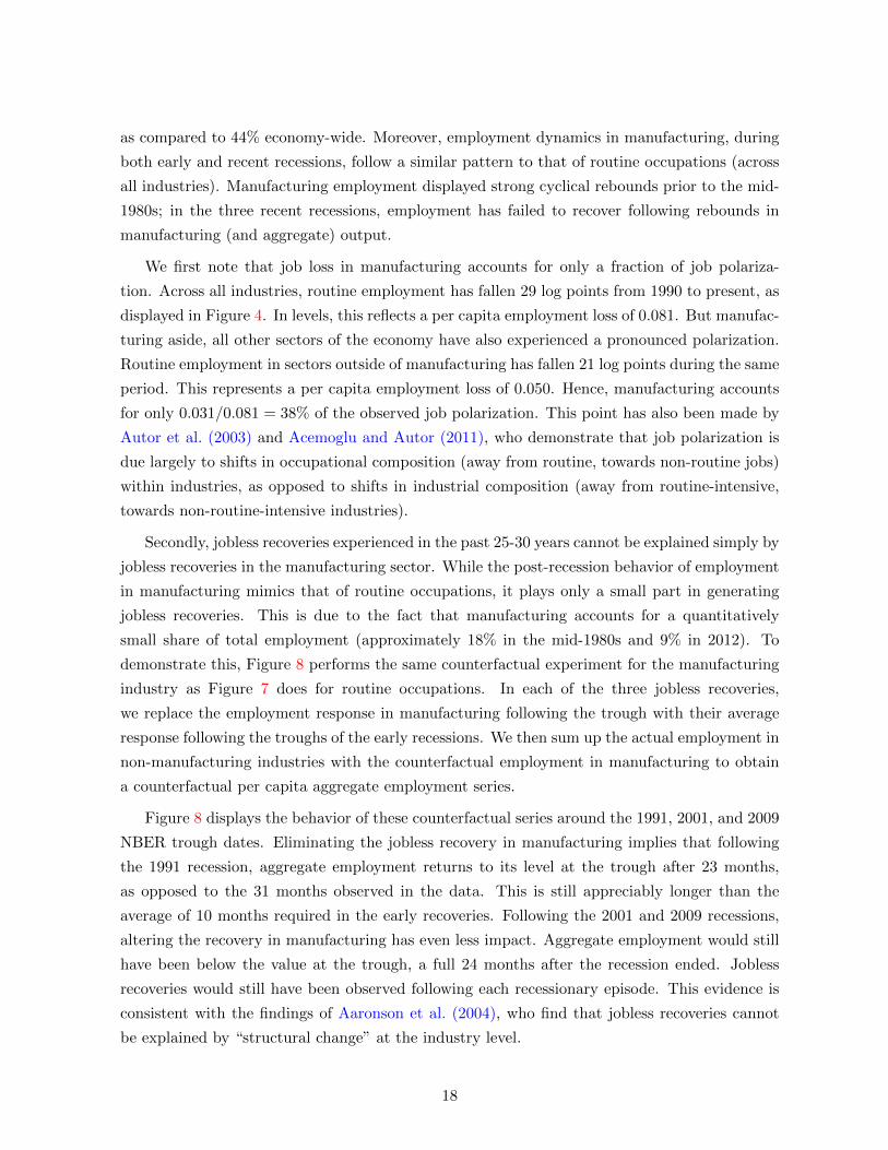
demonstrate this, Figure 8 performs the same counterfactual experiment for the manufacturing

industry as Figure 7 does for routine occupations. In each of the three jobless recoveries,

we replace the employment response in manufacturing following the trough with their average

response following the troughs of the early recessions. We then sum up the actual employment in

non-manufacturing industries with the counterfactual employment in manufacturing to obtain

a counterfactual per capita aggregate employment series.

Figure 8 displays the behavior of these counterfactual series around the 1991, 2001, and 2009

NBER trough dates. Eliminating the jobless recovery in manufacturing implies that following

the 1991 recession, aggregate employment returns to its level at the trough after 23 months,

as opposed to the 31 months observed in the data. This is still appreciably longer than the

average of 10 months required in the early recoveries. Following the 2001 and 2009 recessions,

altering the recovery in manufacturing has even less impact. Aggregate employment would still

have been below the value at the trough, a full 24 months after the recession ended. Jobless

recoveries would still have been observed following each recessionary episode. This evidence is

consistent with the findings of Aaronson et al. (2004), who find that jobless recoveries cannot

be explained by “structural change” at the industry level.

18

Figure 8: Actual and Counterfactual Employment around Recent NBER Recessions: the Man-

ufacturing case

Notes: Actual data from the Bureau of Labor Statistics, Current Employment Statistics Survey;counterfactuals described in Appendix C.

19

Finally, we note that neither phenomena are due to employment dynamics in construction.

With respect to job polarization, of the total job losses in routine occupations from 1990 to

present, only 6% are accounted for by construction. And while not displayed here for brevity,

we have performed the same counterfactual experiment for the construction industry that Figure

8 does for manufacturing. Following each of the recent recessions, replacing the employment

response in construction with their average response following the early recessions has essen-

tially no effect on per capita aggregate employment. Construction plays essentially no role in

accounting jobless recoveries since the industry accounts for a very small share (approximately

5%) of total employment.10

3.4.2 Education

Here, we clarify the role of education in accounting for job polarization and jobless recoveries.

The share of low educated workers in the labor force (i.e., those with high school diplomas or

less) has declined in the last 25 years, and these workers exhibit greater business cycle sensitivity

than those with higher education. It is thus possible to conjecture that the terms “routine” and

“low education” are interchangeable. In what follows, we show that this is not the case.

In particular, it is true that education is correlated with occupation. However, as discussed in

Acemoglu and Autor (2011), educational attainment is more closely aligned with the distinction

between cognitive versus manual occupations, with high (low) educated workers tending to

work in cognitive (manual) jobs. As such, job polarization – the disappearance of employment

in routine occupations relative to non-routine occupations – cannot be explained simply by

the change in educational composition. To make this clear, consider the case of high school

graduates, who make up the majority of low educated workers. In levels, their per capita

employment has fallen 0.057 from 1990 to present. However, this fall is highly concentrated,

with 91% of the loss occurring in routine occupations. In contrast, employment among high

school graduates in non-routine jobs has remained essentially constant, falling by only 0.005

during the polarization period.11

Similarly, jobless recoveries are not simply a phenomenon reflecting the post-recession dy-

namics of low education employment. In particular, business cycle fluctuations for high school

educated workers differ greatly across occupational groups. For these workers, per capita employ-

ment in routine occupations fell 3.6%, 4.0%, and 13.2% in the 1991, 2001, and 2009 recessions,

10See also Charles et al. (2013) for a discussion of housing and manufacturing employment during the mostrecent business cycle boom and bust.

11The importance of the routine/non-routine distinction is further illustrated by the “some college” group –those with more than high school attainment, but less than a college degree. Per capita employment in this grouphas risen 7% since 1990. However, it has only risen in non-routine occupations (by 24%); routine employmenthas actually fallen 7% for the some college group, reflecting polarization among these relatively high educatedworkers. See also the discussion in Autor et al. (2003).

20

respectively. And indeed, it is this group that is disappearing and not recovering: averaged

across the three recessions, employment is down a further 1.5% from the level at the NBER

trough, a full 24 months into the economic recovery. By contrast, employment of high school

graduates in non-routine occupations experience extremely mild contractions – of 0.9%, 0.2%,

and 0.5% in the three recent recessions – and no long term disappearance. Thus, among these

low educated workers, jobless recoveries are only to be found in routine occupations.

4 A Simple Model

In this section, we present a simple analytical model linking the phenomena of job polarization

and jobless recoveries. We show how a simple model can qualitatively capture the following

observations: (a) routine biased technological change (RBTC hereafter) leading to job polariza-

tion, (b) routine job loss being “bunched” in recessions despite a “smooth” RBTC process, (c)

aggregate job loss in recessions being concentrated in routine occupations, (d) jobless recoveries

caused by the disappearance of routine employment, and (e) absent RBTC, non-jobless recov-

eries in routine and aggregate employment. In Subsection 4.3.1 we demonstrate how the key

mechanisms embodied in the model conform with data on transition rates across labor market

states, and how these have changed across pre- and post-job polarization eras.

Our analytical framework is a search-and-matching model of the labor market with occupa-

tional choice and RBTC. The search-and-matching framework of Diamond (1982), Mortensen

(1982), and Pissarides (1985) (hereafter, the DMP framework) is well-suited for our analysis

since it emphasizes the dynamic, multi-period nature of employment and occupational choice.

Our goal is to determine the minimum perturbations to an otherwise standard DMP model that

are required to generate features (a) through (e).

The model’s explicit consideration of frictional unemployment also allows us to address the

recent discussion of shifts in the Beveridge Curve (see, for instance, Weidner and Williams

(2011) and Daly et al. (2012)), as well as “mismatch” in the labor market (see, for instance,

Kocherlakota (2010) and Sahin et al. (2012)) since the end of the Great Recession. Specifically,

we show how jobless recoveries caused by job polarization can cause an outward shift of the

Beveridge Curve. Nonetheless, such an episode need not result in any increased mismatch

between vacancies and unemployed workers.

We present a model with only non-routine cognitive (or “high-skill”) occupations and routine

(“middle-skill”) occupations. RBTC is modelled as a trend increase in the productivity of high-

skill occupations relative to middle-skill occupations.12 In the face of RBTC, middle-skill workers

choose whether to remain in a routine occupation for which they are currently well-suited, or

12See, for instance, Acemoglu and Autor (2011) who document a widening wage gap between high- and middle-skill earnings since about 1980, and a narrowing gap between middle- and low-skill earnings since the 1990s.

21

attempt to become a high-skill worker. If middle-skill workers leave the market for routine

work, then we have a disappearance of middle-skill employment.13 We use this simple model

to illustrate how a temporary, recessionary shock can accelerate this disappearance, and how

recessions during a phase of job polarization can lead to jobless recoveries.

4.1 Description

Workers differ in their ability in performing occupational tasks, and this ability is reflected in

the output in a worker-firm match. Workers are of three types: (1) “high-skill” workers who

have the ability to perform non-routine cognitive tasks, (2) “middle-skill” workers who have the

ability to perform routine tasks but currently lack the ability to perform non-routine cognitive

tasks, and (3) middle-skill workers who are in the process of acquiring the skills to do non-routine

cognitive work. The process of gaining the ability to do high-skill work requires experience on

the job, as emphasized in the learning-by-doing literature. Firms post vacancies for workers of

different types in separate labor markets.

As emphasized in the DMP framework, labor markets feature a search friction in the match-

ing process between unemployed workers and vacancy posting firms. We let θ denote the ratio of

vacancies to unemployed workers, the so-called “tightness ratio,” in a given labor market. The

tightness ratio determines the match probabilities in that market. Let q (θ) denote the proba-

bility that a firm vacancy matches with an unemployed worker (the job filling probability), and

p(θ) be the probability that a worker matches with a vacancy (the job finding probability). We

assume that the matching process has the usual properties, so that p(θ) is a strictly increas-

ing function of θ; q(θ) is strictly decreasing in θ; and q(θ) = p(θ)/θ. As discussed below, the

one crucial perturbation to an otherwise standard DMP model that we consider is allowing the

search friction to be more severe in one labor market relative to the others.

We begin by describing the market for high-skill workers, which is essentially identical to

the model of Pissarides (1985). Firms maintain (or “post”) vacancies to recruit these workers.

Vacancy posting must satisfy the following free entry condition:

κ = βq (θHt) JHt+1. (1)

Here, κ is the cost of maintaining such a vacancy, β is the one-period discount factor, and JH is

the firm’s surplus from being matched with a high-skill worker. Again, q (θH) is the probability

that the firm’s vacancy, posted in the high-skill market, is matched with an unemployed high-

skill worker (the only type of worker searching in this market). We adopt the usual timing

convention whereby matches formed at date t become productive at date t+ 1.

13See also Cortes (2012) and Cortes et al. (2013) for evidence on the quantitative importance of the rise inoccupational switching probabilities during the job polarization period. Note also that our model omits low-skill(i.e. non-routine manual) work; we defer greater discussion of this to Subsection 4.4.

22

Firm surplus is given by:

JHt = fHt − ωHt + β(1− δ)JHt+1, (2)

where fH is the output (or revenue) produced in a high-skill worker-firm match, ωH is the

compensation paid to the worker, and δ is the exogenous separation rate.

An unemployed, high-skill worker receives a flow value of unemployment, z, and matches

with a high-skill vacancy at rate p(θH). If a match occurs, the worker begins employment in

the following period; otherwise she remains unemployed. The present discounted value of being

unemployed for such a worker is:

UHt = z + β [p(θHt)WHt+1 + (1− p(θHt))UHt+1] , (3)

where WH is the value of being a matched, high-skill worker. This latter value is given by:

WHt = ωHt + β [(1− δ)WHt+1 + δUHt+1] . (4)

Worker compensation is determined via generalized Nash bargaining. Let τ represent the

worker’s bargaining weight in a match. In equilibrium, firm surplus is a fraction, (1−τ), of total

match surplus; worker surplus, W −U , is the complementary fraction, τ . Total surplus is simply

TS ≡ J+W−U ; this imposes the free entry condition, with the firm’s value of being unmatched

normalized to zero. We maintain the assumption of Nash bargaining over compensation, with

identical bargaining weight, in all markets in the model.

In the market for routine, middle-skill workers, firms post vacancies such that the free entry

condition holds:

κ = βq (θMt) JMt+1. (5)

The tightness ratio and firm surplus in this market is subscripted with an M to reinforce the

fact that the M market is distinct from the H market. Note also, that the job filling probability,

q(·), as a function of the tightness ratio is identical in this market to the high-skill market.

Middle-skill workers have the choice to search either in the routine market or in an alternative,

“switching market” to become a high-skill worker (described below).

Firm surplus in such a match is given by:

JMt = max {fMt − ωMt + β(1− δ)JMt+1 , 0} . (6)

Here, fM is the output produced in a middle-skill match, and ωM is the compensation paid to

the worker. The firm may choose to separate from the match, if the surplus is non-positive.14

14This is technically a possibility in the high-skill market as well; however, we assume parameter values aresuch that this uninteresting case does not occur.

23

The value function for a middle-skill worker while employed is:

WMt = max {ωMt + β [(1− δ)WMt+1 + δUMt+1] , UMt} . (7)

The worker can endogenously separate from the match if the value of being unemployed, UM ,

exceeds the value of remaining in the match. With Nash bargaining, separations are efficient

since firm and worker surplus in a match are proportional.

When unemployed, the middle-skill worker faces an occupational choice. First, it may choose

to remain in the market for routine work. In this case, the value of unemployment is given by:

UMMt = z + β [p(θMt)WMt+1 + (1− p(θMt))UMt+1] , (8)

where p(θM ) is the job finding rate in the market for routine work. Otherwise, the worker may

search for a job which permits the switching from routine to non-routine occupations:

UMSt = z + β [p̃(θSt)WSt+1 + (1− p̃(θSt))UMt+1] . (9)

Here, p̃(θS) is the job finding rate in the “switching market,” and WS is the value of being

employed in such a match. We assume that the efficiency of the matching technology in the

switching market is less than that of either the H or M market: p̃(·) = εp(·) with ε ≤ 1. We

view this as a natural assumption, as workers seeking to switch occupations are likely to search

less efficiently (for instance, because they have fewer connections in the new occupation) than

those seeking to return to the same occupation.

The unemployed middle-skill worker chooses where to search according to:

UMt = max {UMMt , UMSt} . (10)

Note that in the case of an unsuccessful job search at date t, the worker is free to search in

either market at date t+ 1.

It remains to define the value functions associated with the switching market. The value of

being employed is given by:

WSt = ωSt + β [(1− δ)WHt+1 + δUHt+1] . (11)

When employed in a switching match, workers receive compensation ωS and acquire skills to-

wards becoming a high-skill worker. For simplicity, we assume the worker learns the ability to

perform non-routine cognitive tasks after one period on the job.15 If the match remains intact,

with probability (1−δ), the worker continues as a high-skill worker with value WH . If the match

is separated, with probability δ, she enters the next period as an unemployed high-skill worker,

15It is obviously possible to allow for stochastic or multi-period learning in switching matches; this would notchange the nature of our results.

24

with value UH . Skills that the worker acquires on-the-job are retained when unemployed and can

be applied to future matches; in other words, occupational skill is not firm- or match-specific.

To close the model, the free entry condition in the switching market is given by:

κ = βq̃(θSt)JSt+1, (12)

where

JSt = fSt − ωSt + β(1− δ)JHt+1. (13)

Again, the severity of the search friction is greater in this market relative to the H and M

markets: q̃(·) = εq(·), ε ≤ 1; fS denotes output in a switching match.

To summarize, our model features two skill levels of workers and three labor markets. Un-

employed high-skill workers choose to search in the high-skill market. Unemployed middle-skill

workers choose to search in one of two markets: the middle-skill market (in which case, their

skills remain the same) or the switching market (in which case, employment in a match allows

them to become high-skill). Combining equations (8)-(10), we obtain:

UMt = max {p(θMt) (WMt+1 − UMt+1) , p̃(θSt) (WSt+1 − UMt+1)} . (14)

Hence, this choice depends on the markets’ relative costs (as summarized by the job finding

rates) and benefits (as summarized by the worker surpluses).

Finally, we note that the model has been specified so that the only exogenous elements that

differ across markets are: (i) match productivities, represented as fHt, fMt, and fSt in high-

skill, middle-skill, and switching matches, respectively, and (ii) search frictions, represented as

p(·) and q(·) in the high- and middle-skill markets, and p̃(·) and q̃(·) in the switching market.

Element (i) is an asymmetry across markets that allows us to model RBTC in a simple manner.

Element (ii) is the single, natural asymmetry that the model requires to match all of the facts

and features discussed in the introduction to Section 4.16

4.2 Results

To understand the model’s implications for occupational choice, we begin with a steady state

analysis. We then analyze the model’s perfect foresight dynamics to demonstrate the implica-

tions for job polarization and jobless recoveries.

4.2.1 Steady State

Suppose output in all matches is constant at the values fH , fM , and fS over time. This allows

us to consider a steady state equilibrium in which all worker and firm values are constant over

16As we discuss below in Subsection 4.2.3, alternative approaches exist that deliver the same analytical result;our point is simply that the model requires just one such asymmetry across markets.

25

time. Equilibrium in each market is summarized by the free entry conditions (1), (5), and (12);

we write them here in a generic format for market i as:

κ = qi(θi)β(1− τ)TSi. (15)

The term (1 − τ)TS is simply firm surplus, given Nash bargaining. Hence, the tightness ratio,

θ, is increasing in the profit conditional on being matched, β(1− τ)TS.

High-Skill Market Steady state total surplus in a high-skill match is standard and given

by:

TSH =fH − z − τ̂κθH

1− β(1− δ), (16)

where τ̂ ≡ τ/(1 − τ). The numerator in equation (16) gives the contemporaneous surplus

from a match; this consists of the output (fH) net of the flow value (z) and option value

(τ̂κθH) of foregone unemployment. The total surplus is simply the present discounted value of

contemporaneous surpluses. The value of being an unemployed high-skill worker in steady state

is given by:

UH =z + τ̂κθH

1− β. (17)

Middle-Skill Markets For middle-skill workers, the total surplus and the value of being

unemployed depend on which market the unemployed search in. Consider the case when middle-

skill workers search in the routine market, so that UM = UMM . Steady state total surplus in a

routine match is:

TSM =fM − z − τ̂κθM

1− β(1− δ), (18)

and the value of unemployment is:

UMM =z + τ̂κθM

1− β. (19)

These have the same interpretations given above for the H market.

In a steady state with unemployed middle-skill workers searching in the switching market

(UM = UMS), the value of unemployment is:

UMS =z + τ̂κθS

1− β. (20)

The expression for total surplus in a switching match is best understood in the following form:

TSS = fS − z − τ̂κθS + β [(1− δ)TSH + (UH − UM )] . (21)

The contemporaneous surplus is simply fS − z − τ̂κθS . However, relative to type H and M

matches, the continuation value of a switching match differs in two ways. First, conditional on

26

surviving exogenous separation, the surplus continues as TSH , reflecting the learning of high-

skill tasks. Second, regardless of whether the match survives or not, total surplus involves the

additional term, β(UH − UM ); this reflects a capital gain to the worker from the acquisition of

high-skill ability.

In steady state, the search decision of unemployed type M workers depends on the relative

magnitudes of UMM versus UMS . From equations (19) and (20), this simplifies to the comparison

of θM ≷ θS .

It is easy to see that either steady state can emerge, depending on parameter values. We

first consider a steady state in which the unemployed search in the switching market. To do

this, suppose that fS = fH and ε = 1. This eliminates all asymmetries in exogenous elements

between the high-skill and switching markets, simplifying the analysis. In this case, the following

result obtains.

Proposition 1 Suppose fS > fM . In steady state equilibrium, UMS > UMM .

The proof is contained in Appendix D. The intuition is straightforward. Since output is greater in

switching matches than in routine matches, worker surplus is greater in the S market. Moreover,

because search frictions are identical across markets, the job finding rate is greater in the S

market than in the M market. Hence, unemployed middle-skill workers prefer to search in the

S market since matches arrive at a faster rate, and matches provide greater surplus.

It is also possible that unemployed middle-skill workers would choose to search in the routine

market, even when fS > fM . This occurs when the search friction in the switching market is

sufficiently large relative to that in the routine market.

Proposition 2 Suppose fS > fM . There exists a (unique) cut-off value, ε∗ < 1, such that for

all ε < ε∗, UMM > UMS in steady state equilibrium.

Because the proof is trivial, we do not detail it here for brevity, and make it available upon

request. Intuitively, fS > fM implies that worker surplus in a switching match exceeds that in a

routine match. However, as discussed in relation to condition (14), the value of unemployment

depends also on the probability of entering into a match, the job finding rate. Lower matching

efficiency implies lower job finding rates. Hence, for sufficiently small ε, the cost of facing a lower

job finding rate outweighs the benefit of higher worker surplus in the S market. As a result,

workers prefer to search in the M market.

4.2.2 Job Polarization

We now consider dynamics in an economy that experiences RBTC. Specifically, suppose the

economy starts at date t = 0 in a steady state where middle-skill workers prefer to work and

27

search in the routine, M market. In the initial steady state, productivity is such that fH >

fM > fS . In addition, we follow the logic of the Subsection 4.2.1 and assume that ε is sufficiently

small so that, initially, UMM > UMS and the S market is not operative.

At date t = 1, agents learn that, due to RBTC, productivity in a high-skill match, fH ,

rises at a constant rate to a new value over time; all other match productivities, and crucially,

productivity in a routine match, fM , remains constant. As a result, middle-skill workers even-

tually prefer to search in the S market in order to become high-skilled, and the labor market

polarizes. Given the recursive nature of the model, we can map out the model’s perfect foresight

dynamics.17

As fH rises, so too does the total surplus in S matches. This, of course, is because switching

matches become high-skill matches after one period. From the free entry condition, this implies

that the tightness ratio, θS , rises too. This in turn implies a rise in the value of unemployed

search in the switching market, UMS . Given that RBTC has no effect on productivity in routine

matches, fM , there is little effect on total surplus, TSM , early on and unemployed middle-skill

workers continue to search in that market, UM = UMM .

But as RBTC progresses, and the value of unemployed search in the switching market rises,

the economy reaches a point when UMS > UMM . This initiates the disappearance of routine

employment. Once the economy enters this polarization phase, there is a marked change in

the “occupation of destination” of unemployed middle-skill workers: they switch from searching

solely in the M -market to searching solely in the S-market. As θS continues to rise, so too

does the job finding rate in that market, p̃(θS), and the upgrading of middle-skill to high-skill

workers. In the long-run, routine employment disappears, and the entire workforce becomes

high-skill.

In what follows we illustrate these dynamics in an example. The initial steady state has half

of all workers (working or searching) in the H market, and the remaining half in the M market

(again, the S market is initially not operative).

Figure 9 depicts the perfect foresight paths for UMMt and UMSt. Agents in this example

learn at period 1 that RBTC causes fH to grow at a constant rate over time, reaching a new

steady state level in period 200. Initially, unemployed middle-skill workers prefer to search for

work in the routine market. In period 75, this switches and they prefer searching in the switching

market. This marks the onset of the job polarization era. Even though no observable, discrete

“shock” has occurred to productivity, all unemployed middle-skill workers switch in response

to the “trend” change in relative productivity. This, of course, is accompanied by a change in

vacancy creation: during the polarization era, firms no longer post vacancies in the M market

and post only in the S market.

17Specifically, we first solve for the terminal, post-RBTC steady state. We then work backwards, period-by-period, to the initial steady state, solving for the value functions and tightness ratios along the transition path.

28

Figure 9: Middle-Skill Worker’s Value of Unemployment

Notes: The blue line denotes the value of an unemployed middle-skill worker searching for routineemployment. The green line denotes the value of an unemployed middle-skill worker searching inthe switching market. The red dot indicates the period in which the value of unemployment in theswitching market crosses above that in the routine market.

In this example, total surplus in routine matches, TSM , remains positive even in the terminal

steady state. Hence, during the job polarization era, there is no endogenous separation of

middle-skill matches. The only M -type workers switching from the M market to the S market

are those that find themselves unemployed. Hence, the disappearance of routine employment

happens gradually as such matches exogenously separate at the rate δ; upon separation, all

unemployed middle-skill workers choose to search for a switching match.

Figure 10 depicts the share of H-, S-, and M -type workers in the economy. In periods 1

through 75, the composition of worker types remains unchanged despite the underlying RBTC

trend in relative match productivities: high-skill workers remain as such, and routine workers

have no incentive to switch. But in period 75, all unemployed middle-skill workers leave the

routine market and begin searching in the switching market. In all subsequent periods, workers

who exogenously separate from routine matches also choose to search in the switching market;

routine workers gradually disappear.

4.2.3 Polarization, Recessions, and Jobless Recoveries

It is also possible to see how a recession accelerates the disappearance of routine employment.

In our framework, a recession is modelled as an unanticipated, temporary fall in aggregate

productivity (i.e., a fall in the productivity of all matches).

29

Figure 10: Evolution of Worker Types During Job Polarization

Notes: The process of RBTC begins in period 1. Job Polarization begins in period 75, asmiddle-skill workers leave the routine market for the switching market, and eventually becomehigh-skill workers.

Suppose the process of RBTC is at a stage such that the economy has entered the polarization

era (UM = UMS > UMM ) so that unemployed middle-skill workers search in the switching mar-

ket. If the recessionary fall in productivity is sufficiently large, total surplus in routine matches

becomes non-positive, TSM ≤ 0, while total surplus in all other matches remain positive.18

This is the case that we consider. When TSM ≤ 0, routine matches endogenously separate.

The matched firm prefers to become a vacancy, and the matched routine worker prefers to be

unemployed; in particular, these workers choose unemployment in the S market, in order to

switch occupations.

This is depicted in Figure 11. As in Figures 9 and 10, the disappearance of the routine

18It is easy to see that there always exists a negative productivity shock such that this happens. For simplicity,consider a one-period shock that occurs in the last period before the UMS > UMM switch. This allows us todisregard the S market, which is not yet operative. The total surplus in the two active markets is given by:

TSM = fM − z − τ̂κθM + β(1 − δ)TS′M ,

TSH = fH − z − τ̂κθH + β(1 − δ)TS′H .

The fact that fH > fM (and that the gap is increasing due to RBTC) implies that TSH > TSM at all points intime. Hence, for an additive productivity shock (dropping fH and fM by the same amount in level terms), it iseasy to find a shock that causes TSM ≤ 0, leaving TSH > 0. In the case of a multiplicative shock, one simplyneeds to find a factor, x, such that xfM − z − τ̂κθM + β(1 − δ)TS′M = 0. Applied to the H-type match, it mustbe that xfH − z − τ̂κθH + β(1 − δ)TS′H > 0.

30

Figure 11: Job Polarization Accelerated by Recession

Notes: The process of RBTC begins in period 1. Job Polarization begins in period 75, and isaccelerated by a temporary recession that begins in period 75.

market begins in period 75. To make things exceedingly clear, we introduce an unanticipated,

temporary, negative shock to aggregate productivity in exactly period 75 that lasts for 10 periods.

At the onset of the recession, all unemployed middle-skill workers move from searching in the

M market to the S market; moreover, all employed middle-skill workers endogenously separate

to unemployment in the S market.

Productivity returns to its non-recession level in period 85. At this point, the values of

employment, unemployment, firm surplus, and total surplus in all markets return to their non-

recession, perfect foresight paths. Total surplus in routine matches returns to positive. However,

this is irrelevant as the economy has already entered the job polarization phase where UMS >

UMM . Despite positive total surplus in routine matches, there are no unemployed middle-skill

workers who choose to search in the M market. Hence, in this simple example, all of the

disappearance of routine employment occurs in recessions.

More generally, during an era of job polarization (any period after t = 75 in our example),

recessions accelerate the disappearance of routine jobs. This acceleration occurs not because

recessions change the occupational choice of unemployed M -type workers: once the job polar-

ization era begins, all unemployed middle-skill workers search solely in the S market, regardless

of whether the economy is in boom or recession. Instead, recessions accelerate the disappearance

of routine employment because of the spike in endogenous separations of M -type matches.

31

Moreover, the recovery from such a recession can be jobless. In period 85, aggregate pro-

ductivity returns to its pre-recession level. This implies an immediate jump in match output,

and thus, in aggregate output. However, this is not accompanied by a jump in employment. In

the recession, job separations were concentrated among the middle-skill, routine workers. The

recovery in aggregate employment then depends disproportionately on the post-recession job

finding rate of these workers now searching in the S market.19 If this job finding rate is low, the

rebound in employment will be sluggish: the economic recovery is jobless.

This is precisely the case in our model. The left panel of Figure 12 depicts the dynamics

of aggregate output and employment around the recession. Both are normalized to unity in

the initial period of the recession, period 75. When productivity rebounds in period 85, output

recovers. However, there is no corresponding rebound in employment, as the middle-skill workers

who became unemployed in the recession face low job finding rates in their preferred search

market, the S market.

This low job finding rate is achieved in our model in a simple way: by setting the relative

matching efficiency in the switching market, ε, low. This captures the natural idea that workers

search less efficiently when they are switching occupations than otherwise. Indeed, it is possible

to show that this single asymmetry across labor markets is all that is required to generate a

jobless recovery.

Proposition 3 Suppose ε = 1. Then the model does not exhibit jobless recoveries.

Moreover, this is not the only asymmetry that can generate a jobless recovery in our model.

Allowing for different vacancy posting costs or different Nash bargaining weights across markets

would lead to the same result. These alternatives, as well as the proof of Proposition 3, are

discussed in Appendix D. More broadly, a jobless recovery involves a slow transition into em-

ployment from any source of non-employment. Hence, the middle-skill worker’s time spent in the

S market could be viewed as a stand-in for a temporary spell of labor force non-participation to

relocate or re-train in order to switch occupations. Of course, this would require extending the

standard DMP framework to include an additional labor force state (out of the labor market),

and is beyond the scope of this paper.

4.2.4 No Polarization, No Jobless Recoveries

Here we analyze the effects of a recessionary shock absent job polarization. In such an economy,

middle-skill workers are not searching in the S market when unemployed. As a result, recoveries

19The employment recovery does not depend exclusively on the job finding rate in the S market, however. Thisis because the recession affected productivity in all matches, even high-skill ones. Hence, the recession depressesvacancy creation in the H market; despite the lack of endogenous separations of H-type matches, the recessionincreases the unemployment rate among H-type workers.

32

Figure 12: Recoveries With and Without Job Polarization

Notes: The blue line denotes aggregate output, the red line aggregate employment. Both are normalized to 1in the initial period of recession. A temporary fall in aggregate productivity in period 75 generates a recession;productivity returns in period 85. The left panel displays the case with job polarization, leading to a joblessrecovery. The right panel displays the case with no job polarization, leading to a recovery in both output andemployment.

would not be jobless.

This is illustrated in the right panel of Figure 12. Here we consider an identical model, except

there are no underlying trends in fH . As a result, unemployed high-skill workers search in the

H market and unemployed middle-skill workers search in the M market. No workers choose to

search in the low matching efficiency S market. In period 75 there is a temporary, unanticipated

drop in productivity, lowering match surplus. As before, there is a spike in separations of middle-

skill matches, and vacancy creation falls. Hence, both output and employment fall at the onset

of recession.

But as the right panel makes clear, absent the force for job polarization, there would be no

jobless recovery. When the recession ends, employment rebounds along with output. Indeed,

employment leads output out of the recession; this is because we are studying perfect foresight

paths, and job creation is forward-looking, anticipating the recovery in productivity. Crucially,

because no unemployed workers search in the low efficiency S market, the rebound in job creation

results in a strong rebound in the aggregate job finding rate, and thus, a recovery in employment.

4.3 Labor Market Implications

In this subsection, we document that our model is consistent with a number of key facts regarding

the cyclical behavior of aggregate labor market flows. First, as documented in Section 3.2, the

bulk of the job loss in recessions is in routine occupations. In our model, this is precisely the case

as all endogenous separations occur in M -type matches in the recession. Second, as documented

in Fujita and Ramey (2009) and Elsby et al. (2009), the onset of US recessions feature a spike

33

in the aggregate separation rate; this too occurs in our model.

Third, after the initial spike in separations, employment dynamics are determined by the job

finding rate. In the data, as in our model, jobless recoveries are characterized by a low aggregate

job finding rate, relative to that observed in recoveries of the 1970s and early 1980s. In our

model, the low job finding rate is due to unemployed middle-skill workers who are switching

occupations, and no longer returning routine employment.20 We discuss this in greater detail in

the next subsection.

Fourth, jobless recoveries are associated with outward shifts in the model’s Beveridge Curve.21

This is illustrated in Figure 13, for the case considered in Figure 11 and the left panel of Figure

12. The horizontal axis displays the unemployment rate, u, while the vertical axis displays the

model’s vacancy rate, v. The (u, v) pairs for periods 1 through 74 are displayed as the point

marked as an ‘x’ in the upper-left (northwest) corner. Prior to the job polarization era, la-

bor markets are in steady state: all employed workers are separating from matches at rate δ,

unemployed H-type workers are matching at rate p(θH), and unemployed M -type workers are

matching at rate p(θM ); no workers are searching in the S market.

The recession begins in period 75. This is indicated by the solid diamond in Figure 13. As

productivity in all matches fall, vacancy creation in all markets fall; this, and the spike in endoge-

nous separations of M -type matches, generates a rise in unemployment. The economy moves

to the most southeasterly point in the figure, moving “along” a downward sloping Beveridge

Curve, as is typical in recessions.22

Match productivity returns to trend in period 85, marking the onset of the (jobless) re-

covery. These periods are plotted as the circles. Note that the Beveridge Curve has shifted

outward, indicating a higher unemployment rate at any given vacancy rate. Over time, the

(u, v) observations move to the northwest, mapping out a new Beveridge Curve, as the recovery

progresses.

This shift is due to the compositional change in the pool of vacancies and unemployed

workers. As discussed above, the onset of the recession generates a spike in separations among

middle-skill matches. This generates a dramatic change in the composition of unemployed work-

ers, with a sudden increase in the fraction of M -type workers. In the job polarization era, these

workers search in the S market. Hence, the recession shifts the composition of unemployment

20By construction, this fall is very stark in the model, as workers cease searching in the M market permanently,in favor of the S market, once the economy enters the polarization phase.

21For discussion related to the period following the most recent recession, see for instance Weidner and Williams(2011) and Daly et al. (2012).

22The remaining recessionary periods (periods 76 through 84) are indicated by the hollow diamonds. Vacanciesbegin to rise while unemployment begins to fall. The swift recovery in job creation is due entirely to the fact thatwe study perfect foresight dynamics of our example: agents know that the recession ends in period 85, so thatvacancies are created in anticipation of the return to trend productivity in the near future. In more complicatedexamples where the duration of the recession is uncertain, vacancies remain low throughout the recession.

34

Figure 13: Jobless Recovery and Shift Out of Beveridge Curve

Notes: A temporary fall in aggregate productivity in period 75 (solid diamond) generatesa recession; productivity returns in period 85 (circle).

and vacancies toward the market with low matching efficiency. From the aggregate perspective,

the efficiency of the economy’s matching process has fallen: for any given vacancy rate, workers

find it harder to find matches, resulting in higher unemployment. This generates the outward

shift of the Beveridge Curve.

Finally, we note that jobless recoveries in our model are not accompanied by increased

“mismatch” in the labor market. Though there are a number of working definitions of mismatch

in the literature, the common idea is summarized by Kocherlakota (2010): “Firms have jobs,

but can’t find appropriate workers. The workers want to work, but can’t find appropriate jobs.”

This does not occur in our model. While recessions result in a large number of separations in

middle-skill matches, these unemployed workers choose to search in the switching market. There

are no middle-skill workers searching “inappropriately” for vacancies in the M market that do

not exist. Similarly, because firms are free to create vacancies in any market, firms do not post

vacancies in the M market inappropriately to attract unemployed workers who prefer to become

high-skill workers; new vacancies are created in the S market where unemployed middle-skill

workers are searching. Therefore, there is no more mismatch during a jobless recovery than

there was before.

Obviously, our simple search-and-matching model is not a wholly accurate representation of

the real world. Nonetheless, it presents an environment in which equilibrium arguments result

in jobless recoveries, driven by RBTC and job polarization, without increased mismatch. As

35

such, the model is consistent with the weak evidence for increased mismatch following the most

recent recession (see, for example, Sahin et al. (2012)).

4.3.1 Implications for Labor Market Flows

Our final exercise is to provide further empirical evidence regarding the two key mechanisms

in our model. The first relates to the role of occupational switching in job polarization. The

second relates to the role of job finding rates in generating jobless recoveries. To do so, we study

data on flows across labor market states, and how these have changed as job polarization has

progressed over time.

We analyze the Current Population Survey (CPS) micro-files, from which we obtain monthly

data from 1976 to 2012. In the CPS, households are surveyed for four consecutive months, then

leave the sample during the next eight months, and then are surveyed again for a final four

months. Each household member is uniquely identified. As such, we obtain a longitudinal

record for each person which allows us to study individual labor market experiences over time.

We track monthly transitions across states of employment, unemployment, and labor force non-

participation. When a person is employed, we are able to observe the individual’s occupation

and classify that occupation as either routine or non-routine. When a person is unemployed, we

are able to observe the individual’s most recent occupation.23

With this data, we first consider our model’s emphasis on occupational choice in job polariza-

tion. Once RBTC reaches a critical value, all unemployed routine workers switch occupations.

That is, in the model’s pre-polarization era, unemployed middle-skill workers search in the M

market; in the post-polarization era all unemployed middle-skill workers search in the S market.

Hence, our model predicts a very stark change in the occupational switching rate of unem-

ployed routine workers: prior to job polarization, conditional on finding a job, the probability

of becoming employed in a non-routine occupation is zero; after job polarization begins, the

probability of switching to non-routine employment is unity. Moreover, our model predicts that

this switching rate is acyclical. By definition, UMMt > UMSt in the pre-polarization era, so the

switching rate is always zero; UMSt > UMMt in the post-polarization era, so the switching rate

is always one; this holds regardless of whether the economy is in boom or recession.

These predictions are borne out, qualitatively, in the CPS data. We compute the occupa-

tional switching rate for unemployed routine workers, conditional on finding a job. Between any

two months t−1 and t, this is simply the ratio of unemployed individuals in t−1 with a previous

routine occupation who transition to employment in a non-routine occupation in t, relative to

the number unemployed individuals in t− 1 with a previous routine occupation who transition

23Unfortunately, the CPS does not record the most recent occupation for those out of the labor force. For acomplete description of the longitudinal data, see Nekarda (2009) and Cortes et al. (2013).

36

Figure 14: Fraction of Job Finding Transitions for Unemployed Routine that are to Non-Routine

Employment

Notes: Data from the Bureau of Labor Statistics, Current Population Survey. See Ap-pendix A for details.

to employment in any occupation in t. This switching rate is plotted in Figure 14. Because the

monthly transition rate data are noisy, the switching rate has been band pass filtered to remove

fluctuations at frequencies higher than 18 months.

As can be seen, the probability that an unemployed routine worker switches to a non-routine

job (either cognitive or manual) when he or she finds employment is rising as job polarization has

unfolded over time. In fact, from 1976 to present the switching rate has increased approximately

45%.24 Moreover, as predicted by our model, occupation switching is not only rising, but is also

acyclical. While monthly transition rates exhibit noticeable high frequency fluctuations (even

after band pass filtering), these are not related to periods of boom, recession, and recovery.

When we consider the business cycle components of the switching rate and monthly RGDP

(fluctuations with frequency between 18 and 96 months), we find the correlation to be −0.05.

Hence, the switching rate in the data displays no clear cyclical pattern.

It is worth noting that the rising switching rate in Figure 14 does not simply reflect greater

24Recall in our model, middle-skill workers are switching “up,” from routine jobs to higher productivity, non-routine cognitive jobs. Taking our model literally would imply a rising switching rate for unemployed routineworkers to non-routine cognitive employment. Though not pictured here for brevity, we find that this predic-tion holds in the data as well; in fact, the switching rate into non-routine cognitive employment increases byapproximately 80% during the same time period. By contrast, the switching rate into non-routine manual jobshas increased by only 7%. Hence, job polarization has been associated with essentially no change in occupationalswitching of unemployed routine workers “down” in the CPS data.

37

“churning” between routine and non-routine occupations. Though not displayed for brevity, the

switching rate of unemployed non-routine workers to routine occupations during the same time

period has fallen by 37%.25 To gain greater insight into this, note that this switching rate is

the number of unemployed workers with a previous non-routine occupation who transition to

routine employment, divided by the number of unemployed non-routine workers who transition

to either routine or non-routine employment. Dividing both the numerator and denominator by

the number of unemployed non-routine workers, the switching rate can be expressed as:

switching rateUNR =ρUNR,R

ρUNR,R + ρUNR,NR, (22)

where ρUNR,R is the job finding rate of unemployed non-routine workers into routine employ-

ment, and ρUNR,NR is the job finding rate of unemployed non-routine workers into non-routine

employment. We find that the falling switching rate of unemployed non-routine workers is due to

a change in both job finding rates. Specifically, averaged across pre- and post-polarization eras:

(i) ρUNR,R has fallen, while (ii) ρUNR,NR has risen. Likewise, the switching rate of unemployed

routine workers to non-routine occupations can be expressed as:

switching rateUR =ρUR,NR

ρUR,R + ρUR,NR, (23)

where ρUR,NR is the job finding rate of unemployed routine workers into non-routine employ-

ment, and ρUR,R is the job finding rate into routine employment. The rising switching rate of

unemployed routine workers in Figure 14 is also due to a change in both job finding rates. Av-

eraged across pre- and post-polarization eras: (i) ρUR,NR has risen, while (ii) ρUR,R has fallen.

Hence, job polarization has exhibited an important change in the “occupational direction” of job

finding: job finding rates— for all unemployed workers, regardless of previous occupation—into

routine jobs is falling, while job finding rates into non-routine jobs is rising.26,27

The second model implication that we investigate relates to jobless recoveries. As discussed

in Subsection 4.2.4, absent job polarization, recessions are followed by strong employment re-

coveries. This is because routine workers displaced in a recession choose to return to their

25The switching rate of unemployed non-routine cognitive workers to routine jobs has fallen by 76%.26In Cortes et al. (2013), we further analyze the changes in job finding rates, and other key labor market

transition rates, observed since job polarization. Using standard decomposition techniques, we study the extentto which these changes are accounted for by changes in demographic composition (so called, explained effects) orchanges in the behavior of individuals with particular demographic characteristics (unexplained effects). We findthat the changes in job finding rates into both routine employment and non-routine employment are overwhelmingdue to changes in unexplained effects.

27While our baseline model is able to address the occupational direction of job finding of unemployed routineworkers, it cannot do so for unemployed non-routine workers. This is because non-routine, H-type workers alwayschoose to remain in the H market. This can be addressed, however, with a simple extension of the model.Suppose that upon separation from a match, H-type workers face a constant, exogenous probability of losingtheir skill. Upon skill loss, such workers become unemployed M -type workers (with previous non-routine jobs).Thus, prior to job polarization all such workers choose to switch occupations and search in the M market. Butin the polarization era, these unemployed workers choose to return to their previous occupation and search in theS market. Hence, this extended version of the model would capture the change in the occupational direction ofjob finding for all unemployed workers found in the data, without altering any of the substantive predictions.

38

previous occupation, and search in the high efficiency M market. When the recession ends and

job creation rebounds, so too does the job finding rate into routine occupations. But this is

not the case after the onset of polarization. Routine workers displaced in a recession choose to

switch occupations. When the recession ends and job creation rebounds, vacancies are posted

in the low efficiency S market. As a result, the recovery in the aggregate job finding rate is

much weaker. Jobless recoveries in our model are due to the lack of recovery in job finding into

routine occupations.

This prediction is consistent with the data as well. To show this, we perform a counterfactual

exercise with the job finding rate into routine occupations, similar to that considered in Subsec-

tion 3.3. To understand this, consider the following law-of-motion describing the evolution of

routine employment:

Rt+1 = NRtρNR,Rt + URtρ

UR,Rt + UNRtρ

UNR,Rt +NLFtρ

NLF,Rt

+Rt(1− ρR,NRt − ρR,UR

t − ρR,NLFt ). (24)

Here, ρX,Yt denotes the transition rate between dates t and t + 1, from labor market state X

to labor market state Y , and R and NR denote per capita employment in routine and non-

routine occupations, respectively. Similarly, UR and UNR denote per capita unemployment

with previous job in either the routine or non-routine occupational groups, respectively. Finally,

NLF denotes non-participation in the labor force. Hence, the evolution of routine employment

is governed by the inflows from non-routine employment, unemployment, and non-participation,

relative to the reverse outflows. Though not displayed here, analogous laws-of-motion govern

the evolution of NR, UR, UNR, and NLF .

Our interest is in whether jobless recoveries would have occurred after recent recessions if the

post-recession behavior of job finding rates into routine employment had behaved as they did

following the early recessions. For the 1991, 2001, and 2009 episodes, we generate counterfactual

time series for R, NR, UR, UNR, and NLF using equation (24) and the four analogous laws-

of-motion. In each of these laws-of-motion, we replace the observed response of the transition

rates from unemployment into routine employment—ρUR,R and ρUNR,R—with counterfactual

values. These counterfactual values replicate the strong rebound in the job finding rates into

routine jobs exhibited following the 1982 recession.28 We then sum up R and NR generated

in this manner to obtain a counterfactual series for aggregate employment in each recessionary

episode. The behavior of these series are displayed in Figure 15. Further details regarding the

construction of the counterfactuals is discussed in Appendix C.

Figure 15 makes clear that if job finding into routine occupations had rebounded as it did

in the 1982 recovery, we would not have observed jobless recoveries in either the 1991 or 2001

28Because the CPS micro-data are only available beginning in 1976, we are unable to observe the behavior ofjob finding rates at the occupational level in the recoveries following the 1970 and 1975 recessions.

39

Figure 15: Actual and Counterfactual Employment around Recent NBER Recessions: Job

Finding Rates

Notes: Data from the Bureau of Labor Statistics, Current Population Survey; counterfactuals de-scribed in Appendix C.

40

episode. Aggregate employment would have recovered beyond its value at the NBER trough date

shortly after the end of each recession. In the case of 2009, the turn around in employment would

have been similarly quick. However, within the 24 month period, the counterfactual exhibits

no clear recovery beyond its NBER trough value.29 Nonetheless, restoring the recovery in job

finding into routine employment would have resulted in a gain of approximately 2% in aggregate

employment relative to its observed value, and prevented its continued decline in the recovery

period. Hence, consistent with our model, we find an important role in the lack of recovery in

job finding rates into routine occupations in accounting for the jobless recovery phenomenon.

4.4 Summary

To summarize, our simple model generates a number of the key features characterizing the US

labor market. It predicts that the disappearance of routine employment is bunched in recessions

despite a gradual, trend process in RBTC. In recessions, job losses are concentrated in routine

occupations. Following recessions, recoveries are jobless and caused by the disappearance of

routine employment. This is due to a low job finding rate among those who are displaced

following a recession. In our model, this occurs for unemployed middle-skill workers who switch

occupations. Absent job polarization, unemployed workers would not switch occupations, and

the recovery would not be jobless.

To match these facts, our model takes an otherwise standard search-and-matching framework

and augments it in two ways. First, we allow the trends in match productivities to differ

across H-, M -, and S-type matches, to capture routine biased technological change and job

polarization. Second, we allow the severity of search frictions to differ across labor markets,

generating the lower job finding rate for workers who switch occupations. We find that these

key mechanisms of our model are consistent with data on micro-level labor market flows.

We note that because our model is so simple, it generates a number of overly stark predic-

tions. For instance, once the job polarization era begins, a single recession generates a complete

disappearance of routine jobs. This obviously is not the case in the data, as each of the 1991,

2001, and 2009 recessions has resulted in successive reductions in routine employment. However,

this shortcoming is easily remedied by introducing heterogeneity among middle-skill workers,

either in their productivity in routine matches, or in their ability to acquire the skills to become

a non-routine cognitive worker. This would also dampen the stark increase in occupational

switching predicted by the model, discussed in Subsection 4.3.1: instead of jumping discretely

from zero to unity, the switching rate would increase more gradually, as in Figure 14. Finally,

we note that our model features only switching from middle-skill to high-skill occupations due

to RBTC, with no treatment of low-skill (non-routine manual) workers. But as discussed in

29This is, perhaps, not surprising given the nature of the Great Recession; see our discussion of Figure 7 andin footnote 9.

41

Subsection 4.3.1, job polarization has not been accompanied by an increase in switching from

routine to non-routine manual jobs. As such, we believe that modeling low-skill workers is not of

first-order importance in understanding the link between job polarization and jobless recoveries.

5 Conclusions

In the last 25 to 30 years the US labor market has been characterized by job polarization and

jobless recoveries. In this paper we demonstrate how these are related. We first show that the

loss of middle-skill, routine employment is concentrated in economic downturns. Second, we

show that job polarization accounts for jobless recoveries. This is based on the fact that almost

all of the contraction in aggregate employment during recessions can be attributed to job losses

in routine occupations (that account for a substantial fraction of total employment), and that

jobless recoveries are observed only in these disappearing jobs since polarization began.

We then propose a simple search-and-matching model of the labor market with occupational

choice to rationalize these facts. We show how a trend in routine-biased technological change can

lead to job polarization that is concentrated in downturns, and recoveries from these recessions

that are jobless. Moreover, we find that the model captures a number of key facts regarding

labor market flows.

These findings illustrate how tenuous it can be to dichotomize “trend” and “cycle” in eco-

nomic analysis. The nature of job polarization and the disappearance of routine employment—a

long-run, or “trend” phenomenon—is informed by an analysis of its business cycle properties.

Moreover, an understanding of jobless recoveries—a “cyclical” phenomenon—requires consider-

ation of the job polarization trend in the labor market.

42

Appendix: For Online Publication

A Data Sources

A.1 Aggregate Data

The population measure is the civilian non-institutional population, 16 years and over, takenfrom the Current Population Survey, Bureau of Labor Statistics. Aggregate employment is totalemployment within this population. Estimates of RGDP at a monthly frequency are those ofJames Stock and Mark Watson (http://www.princeton.edu/ mwatson/mgdp gdi.html). Thesedata end in June 2010; data from July 2010 are interpolated from quarterly RGDP data, takenfrom the FRED Database, Federal Reserve Bank of St. Louis.

In Subsection 3.4, data for industrial employment are from the Current Employment Statis-tics survey of the BLS, taken from the FRED Database. Aggregate employment refers to “allemployees: total nonfarm,” manufacturing employment is “all employees: manufacturing,” andconstruction employment is “all employees: construction.” Data for employment delineated byeducation and occupation are from 1989 to 2012 and were obtained from the Basic MonthlyFiles of the CPS, from the NBER website.

A.2 Disaggregated Data

We consider an occupational classification system that provides ease of data access and repli-cation, and allows for the most comprehensive time series coverage possible, extending backto 1967. Beginning in 1983, our classification is based on the categorization of occupations inthe 2000 Standard Occupational Classification system. Specifically, data for January 1983 toDecember 2013 are taken from FRED. Non-routine cognitive workers are those employed in“management, business, and financial operations occupations” and “professional and relatedoccupations”. Routine cognitive workers are those in “sales and related occupations” and “of-fice and administrative support occupations”. Routine manual occupations are “productionoccupations”, “transportation and material moving occupations”, “construction and extractionoccupations”, and “installation, maintenance, and repair occupations”. Non-routine manualoccupations are “service occupations”.

Data on employment at the occupational group level from July 1967 to December 1982 istaken from the Employment and Earnings, Bureau of Labor Statistics, various issues. Non-routine cognitive workers are those employed in “professional and technical” and “managers,officials, and proprietors” occupations. Routine cognitive workers are those classified as “clericalworkers” and “sales workers”. Routine manual workers are “craftsmen and foremen”, “oper-atives”, and “nonfarm labourers”. Non-routine manual workers are “service workers”. “Farmworkers” (farmers, farm managers, farm labourers and farm foremen) are excluded from theemployment data at the occupational level.

Finally, we note that employment at the occupational group level displays a break between1982 and 1983. This is due to the extensive reclassification of occupations undertaken withthe 1980 Census codes (see, for instance, Rytina and Bianchi (1984) and Meyer and Osborne

43

http://www.princeton.edu/~mwatson/mgdp_gdi.html

(2005)), and implemented in the CPS beginning in January 1983.30 As such, we have adjustedthe data prior to 1983 to remove the discontinuity. Because the adoption of the 1980 occupationcodes occurs only one month from the start of the recovery following the 1982 recession (NBERtrough date on November 1982), the timing of the break does not affect our analysis regardingthe nature of recoveries in employment.

B Robustness

B.1 Classifying Routine Occupations

Here we demonstrate that the key results of our analysis are robust to various definitions ofper capita employment in routine occupations. Specifically, we show that the key “staircase”pattern of routine employment observed in the past 25 years that is responsible for both of ourfindings is a robust feature of the data.

The job polarization literature considers a number of alternative methods to classify em-ployment at the occupational level. Perhaps the most comprehensive is that of Autor andDorn (2012), who first take the Census Occupation Codes from 1970, 1980, 1990, and 2000and map them into a single, consistent set of occupation codes. This “crosswalk” of occu-pation codes is based on the work of Meyer and Osborne (2005). These consistent occupa-tions are then allocated to occupational groups. They generate six broad categories based onan occupation’s degree of emphasis on abstract (i.e., cognitive), routine, and manual tasks:(1) Managers / Professional / Technician / Finance / Public Safety, (2) Production / Craft, (3)Transport / Construction / Mechanic / Mining / Farm, (4) Machine Operators / Assemblers, (5)Clerical / Retail Sales, and (6) Service.

Autor and Dorn (2012) find that groups (2) through (5) are those with routine task usagegreater than the average across all occupations. Hence, one definition of routine occupationswould be these occupational groups. And indeed, our classification system is one in whichroutine occupations are essentially identical to such a definition. Specifically, our non-routinecognitive occupations are group (1), routine manual occupations are groups (2) through (4),routine cognitive occupations are group (5), and non-routine manual occupations are group(6).31 Hence, redoing our analysis defining routine occupations as Autor and Dorn (2012)’sgroups (2) through (5) generates essentially identical results.

A second alternative definition can be derived from the routine task-intensity index, or RTI,derived in Autor and Dorn (2012). Conceptually, the RTI identifies those occupations that havethe greatest routine task emphasis relative to abstract and manual tasks. Based on this measure,routine occupations are those in groups (2), (4) and (5); despite the fact that occupations ingroup (3) involve more routine task emphasis than the average, they are not considered routinebased on the RTI because of their high degree of manual tasks.

The first panel of Figure 16 displays the dynamics of our benchmark measure of per capita

30This is true of any occupational classification system, including the one we consider and that of Autor andDorn (2012).

31In particular, using their consistent occupation codes, we find that of the 330 occupations considered by Autorand Dorn (2012), the two classification systems differ with respect to the routine/non-routine delineation for only15 occupations.

44

routine employment since the job polarization era.32 The second panel displays the measurebased on the RTI. As is obvious, both measures display the key staircase pattern with routineemployment loss concentrated in recessions.

The third panel of Figure 16 further demonstrates robustness; in this case we remove theconstruction-related occupations from our baseline measure of routine occupations. This is moti-vated by the fact that construction is highly sensitive to the business cycle, and has experiencedno long-run decline as a share of total employment. Again, we find that key staircase patternobserved in the other measures of per capita routine employment remain.

Finally, the fourth and fifth panels plot the per capita employment dynamics of routinecognitive and routine manual occupations, respectively, since the job polarization era. As isclear, both cognitive and manual occupations are disappearing over time, and job loss in bothgroups is concentrated in recessions.

B.2 Business Cycle Snapshots: 3 Occupational Groups

Figure 17 plots per capita employment for the routine, non-routine cognitive, and non-routinemanual occupational groups around NBER recessions.

32Again, a measure based on Autor and Dorn (2012)’s groups (2) through (5) would be essentially identical.

45

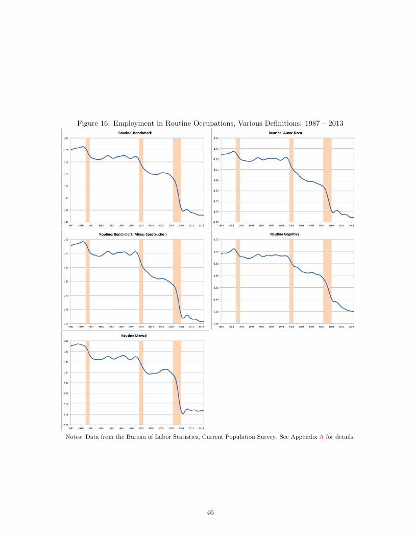
Figure 16: Employment in Routine Occupations, Various Definitions: 1987 – 2013


46

Figure 17: Occupational Employment around Early and Recent NBER Recessions


47

C Counterfactuals

C.1 Subsection 3.3

Using the data for routine occupations displayed in Figure 5, we derive the percentage deviationin employment for the 24 months following the trough of each of the early recessions. Wethen take the average of these deviations and refer to this as the “average response” of routineemployment during early recoveries. This is displayed as the (last half of the) solid line in theupper-left panel of Figure 18. In the 1991, 2001, and 2009 recessions, we replace the post-troughdynamics of routine employment with a re-scaled version of the average response. In particular,we re-scale the average response to match the magnitude of the fall in actual routine employmentwithin the first 5 months of the trough. We choose 5 months, since this is the turning point ofthe average response.

The counterfactual for routine employment is displayed for the example of the 2009 recessionas the hatched line in the upper-left panel of Figure 18. Because the actual fall after the 2009trough was greater than that in the average of the early recessions, the average response had tobe magnified. After 11 months, the average response turns positive. The magnification factorwould then imply a very sharp rebound in the counterfactual. Hence, to be conservative, we setthe counterfactual for months 12 through 24 to be exactly the average response. In the casesof the 1991 and 2001 recessions, the average response fell more sharply than did actual routineemployment. In these cases, the counterfactual was derived by attenuating the average responseby the appropriate factor. To be conservative on the strength of the recovery, after the averageresponse turns positive, we maintained the attenuation factor.

These counterfactuals in log deviations were then used to derive counterfactuals for routineemployment levels. These were then added to the actual employment levels in non-routineoccupations to obtain counterfactual aggregate employment series. These counterfactuals in theaggregate were then expressed as log deviations from their value at the recession troughs toobtain Figure 7.

Finally, in the upper-right, lower-left panel, and lower-right panels of Figure 18, we presentthe results of the same counterfactual experiment for the 1970, 1975, and 1982 recessions. Thesepanels demonstrate that the nature of the early recoveries – which were not jobless – are notfundamentally altered by the exercise. That is, they continue to display recoveries in aggregateemployment with roughly the same magnitude and timing.

C.2 Subsection 4.3.1

For the recent recessionary episodes, we let R, NR, UR, UNR, and NLF evolve as observeduntil the NBER trough date. Counterfactuals for these five time series are generated as follows.

From the 1982 recessionary episode, we are able to observe the job finding rate from: (i)unemployment with a previous routine occupation into employment in a routine occupation,ρUR,R; and (ii) unemployment with a previous non-routine occupation into employment in aroutine occupation, ρUNR,R. From this data, we compare the growth rate of these job findingrates from the 1982 recession to the 24 month period following the trough date. In particular,because the CPS transition rate data are noisy and exhibit pronounced high frequency fluctua-tions, we compute a “growth factor” for ρUR,R as the ratio of its average value in the 24 months

48

Figure 18: Constructing Counterfactual Employment

following the trough date to its average value during the recession. We compute a growth factorfor ρUNR,R in the 1982 recovery period in the same manner.

For each of the 1991, 2001, and 2009 episodes, we generate counterfactual time series for the24 month recovery period using equation (24) and the four analogous laws-of-motion forNR, UR,UNR, and NLF . In the laws-of-motion, we replace the observed values of ρUR,R and ρUNR,R

with counterfactual ones, leaving all other transition rates the same.33 These counterfactualvalues for the job finding rates into routine employment are constructed by multiplying theobserved average values in each recession with their respective growth factors. This allows us toreplicate the recoveries in ρUR,R and ρUNR,R exhibited following the 1982 recession. We thensum up the counterfactual R and NR series to obtain counterfactual aggregate employmentseries for the recent recessionary episode.

D Derivations for Section 4

D.1 Proof of Proposition 1

The proof is by contradiction. Suppose UMM > UMS so that the unemployed search in theroutine market. From equations (19) and (20) this implies that θM > θS . From the free entry

33This implies that the counterfactual exercise also adjusts the probabilities of remaining unemployed, ρUR,UR

and ρUNR,UNR, to ensure that transition probabilities sum to one.

49

condition (15), this implies that TSM > TSS , or:

fM − z − τ̂κθM + β(1− δ)TSM > fS − z − τ̂κθS + β(1− δ)TSH + β(UH − UM ). (25)

Rewriting:

[fM − fS + τ̂κ(θS − θM )] + [β(1− δ)(TSM − TSH)] + β(UM − UH) > 0. (26)

The first term in square brackets [fM − fS + τ̂κ(θS − θM )] < 0 by assumption. Given equations(16) through (19), it is easy to show that (TSM − TSH) < 0 and (UM − UH) < 0. Hence, theleft-hand side of equation (26) is negative, a contradiction.

D.2 Proof of Proposition 3

We first demonstrate that ε < 1 allows for jobless recoveries due to job polarization. Firstnote that a jobless recovery in our model requires a low job finding rate for unemployed M -typeworkers in the S market relative to the M market. That is, it requires p̃(θSt) ≡ εp(θSt) < p(θMt).

Simultaneously, our model features UMSt > UMMt in the job polarization phase. Fromequations (8) and (9), this implies:

z + β [p̃(θSt)WSt+1 + (1− p̃(θSt))UMt+1] > z + β [p(θMt)WMt+1 + (1− p(θMt))UMt+1] (27)

p̃(θSt)(WSt+1 − UMt+1) > p(θMt)(WMt+1 − UMt+1) (28)

p̃(θSt)τ̂JSt+1 > p(θMt)τ̂JMt+1 (29)

θStq̃(θSt)τ̂JSt+1 > θMtq(θMt)τ̂JMt+1 (30)

θSt > θMt. (31)

Going from the second line to the third uses Nash bargaining. Going from the third to thefourth uses the definition of the matching function. Going from the fourth to the fifth uses thefree entry conditions. If ε ≥ 1, equation (31) would imply a higher finding rate in the S marketrelative to the M market. Hence, ε < 1 is required to simultaneously satisfy p̃(θSt) < p(θMt)and equation (31).

From here, it is easy to see how introducing other asymmetries would also allow the modelto generate a jobless recovery. For instance, suppose ε = 1 (so that p̃(·) = p(·)), but allow theNash bargaining weight in the S market, τS , to be greater than that in the other markets, τ , sothat τ̂S > τ̂ . In this case, equation (31) would be replaced by:

τ̂SθSt > τ̂θMt, (32)

and it would still be possible to satisfy this with p(θSt) < p(θMt).

Finally, suppose that both ε = 1 and τS = τ , but κS > κ. In this case, equation (31) wouldbe replaced by:

κSθSt > κθMt, (33)

and it would still be possible to satisfy this with p(θSt) < p(θMt).

50

References

Aaronson, D., E. R. Rissman, and D. G. Sullivan (2004). Can sectoral reallocation explain the

jobless recovery? Economic Perspectives, Federal Reserve Bank of Chicago 28 (2), 36–49.

Acemoglu, D. (1999). Changes in unemployment and wage inequality: An alternative theory

and some evidence. American Economic Review 89 (5), 1259–1278.

Acemoglu, D. and D. Autor (2011). Skills, tasks and technologies: Implications for employ-

ment and earnings. In O. Ashenfelter and D. Card (Eds.), Handbook of Labor Economics,

Volume 4B, Chapter 12, pp. 1043–1171. Elsevier.

Autor, D. (2010, April). The Polarization of Job Opportunities in the U.S. Labor Market:

Implications for Employment and Earnings. Center for American Progress and The Hamilton

Project.

Autor, D. H. and D. Dorn (2012). The growth of low skill service jobs and the polarization of

the us labor market. American Economic Review , forthcoming.

Autor, D. H., L. F. Katz, and M. S. Kearney (2006). The polarization of the u.s. labor market.

American Economic Review: Papers & Proceedings 96 (2), 189–194.

Autor, D. H., F. Levy, and R. J. Murnane (2003). The skill content of recent technological

change: An empirical exploration. Quarterly Journal of Economics 118 (4), 1279–1333.

Bernanke, B. S. (2003). The jobless recovery. http://www.federalreserve.gov/boarddocs/speeches/

2003/200311062/default.htm.

Bernanke, B. S. (2009). On the outlook for the economy and policy.

http://www.federalreserve.gov/newsevents/speech/bernanke20091116a.htm.

Brynjolfsson, E. and A. McAfee (2011). Race Against The Machine: How the Digital Revolution

is Accelerating Innovation, Driving Productivity, and Irreversibly Transforming Employment

and the Economy. Digital Frontier Press.

Charles, K. K., E. Hurst, and M. J. Notowidigdo (2013, April). Manufacturing decline, housing

booms, and non-employment. University of Chicago.

Christiano, L. J. and T. J. Fitzgerald (2003). The band pass filter. International Economic

Review 44, 435–465.

Cortes, G. M. (2012, October). Where have the routine workers gone? a study of polarization

using panel data. University of Manchester.

51

Cortes, G. M., N. Jaimovich, C. J. Nekarda, and H. E. Siu (2013, November). The micro and

macro of disappearing routine jobs: a flows approach. University of British Columbia.

Daly, M. C., B. Hobijn, A. Sahin, and R. G. Valletta (2012). A search and matching approach

to labor markets: Did the natural rate of unemployment rise? Journal of Economic Perspec-

tives 26 (3), 3–26.

Diamond, P. A. (1982). Aggregate demand management in search equilibrium. Journal of

Political Economy 90 (5), 881–894.

Elsby, M. W. L., R. Michaels, and G. Solon (2009). The ins and outs of cyclical unemployment.

American Economic Journal: Macroeconomics 1 (1), 84–110.

Firpo, S., N. M. Fortin, and T. Lemieux (2011, February). Occupational tasks and changes in

the wage structure. University of British Columbia.

Fujita, S. and G. Ramey (2009). The cyclicality of separation and job finding rates. International

Economic Review 50 (2), 415–430.

Goos, M. and A. Manning (2007). Lousy and lovely jobs: The rising polarization of work in

britain. Review of Economics and Statistics 89 (1), 118–133.

Goos, M., A. Manning, and A. Salomons (2009). Job polarization in europe. American Economic

Review: Papers & Proceedings 99 (2), 58–63.

Goos, M., A. Manning, and A. Salomons (2011, November). Explaining job polarization: The

roles of technology, offshoring and institutions. University of Leuven.

Gordon, R. J. and M. N. Baily (1993). The jobless recovery: Does it signal a new era of

productivity-led growth? Brookings Papers on Economic Activity 1993 (1), 271–316.

Groshen, E. L. and S. Potter (2003). Has structural change contributed to a jobless recovery?

Current Issues in Economics and Finance, Federal Reserve Bank of New York 9 (8), 1–7.

Kocherlakota, N. (2010, August). Inside the FOMC.

http://www.minneapolisfed.org/news events/pres/speech display.cfm?id=4525.

Meyer, P. B. and A. M. Osborne (2005). Proposed category system for 1960-2000 census occu-

pations. Bureau of Labor Statistics Working Paper 383.

Mortensen, D. T. (1982). Property rights and efficiency in mating, racing, and related games.

American Economic Review 72 (5), 968–979.

Nekarda, C. J. (2009, May). A longitudinal analysis of the current population survey: Assessing

the cyclical bias of geographic mobility.

52

Pissarides, C. A. (1985). Short-run equilibrium dynamics of unemployment, vacancies, and real

wages. American Economic Review 75 (4), 676–690.

Rytina, N. F. and S. M. Bianchi (1984). Occupational reclassification and changes in distribution

by gender. BLS Monthly Labor Review 107 (3), 11–17.

Sahin, A., J. Song, G. Topa, and G. L. Violante (2012, August). Mismatch unemployment.

NBER Working Paper No. 18265.

Schreft, S. L. and A. Singh (2003). A closer look at jobless recoveries. Economic Review, Federal

Reserve Bank of Kansas City Second Quarter, 45–72.

Stein, R. L. (1967). New definitions for employment and unemployment. Employment and

Earnings and Monthly Report on the Labor Force 14 (2), 3–27.

Weidner, J. and J. C. Williams (2011). What is the new normal unemployment rate? FRBSF

Economic Letter 2011-5.

53

The Trend is the Cycle: Job Polarization and Jobless ... · The Trend is the Cycle: Job...

Documents

Transcript of The Trend is the Cycle: Job Polarization and Jobless ... · The Trend is the Cycle: Job...