The Term Structure of Expected Bond Returns*

Zvika Afik The Guilford Glazer Faculty of Business and Management

Ben-Gurion University of the Negev, Israel afikzv@bgu.ac.il

Simon Benninga Faculty of Management

Tel Aviv University, Israel benninga@post.tau.ac.il

This version: January 3, 2012

Abstract We present a discrete time model of expected bond returns (EBR). These are ex-ante expectations implied by the market prices and the data set available when bond prices are quoted. The model can be used to estimate the rating-adjusted EBR, its risk premium components, including a certainty equivalence premium which is related to the systematic risk of the CAPM. We implement the model using corporate bond transaction data from the United States and a rating agency transition matrix to extract the zero-coupon term structure of EBR and its components and the term structure of risk-neutral default probabilities.

JEL Classification: G12, G24, G32, G33

Keywords: expected returns, corporate bonds, credit risk

* This paper is based on Zvika Afik’s dissertation at Tel Aviv University. We thank Edward Altman, Gady Jacoby and Fan Yu for helpful comments. Responsibility for the paper is of course ours. We have benefited from a grant from the Israel Institute of Business Research at Tel Aviv University.

The Term Structure of Expected Bond Returns*

Abstract We present a discrete time model of expected bond returns (EBR). These are ex-ante expectations implied by the market prices and the data set available when bond prices are quoted. The model can be used to estimate the rating-adjusted EBR, its risk premium components, including a certainty equivalence premium which is related to the systematic risk of the CAPM. We implement the model using corporate bond transaction data from the United States and a rating agency transition matrix to extract the zero-coupon term structure of EBR and its components and the term structure of risk-neutral default probabilities.

1

The Term Structure of Expected Bond Returns

1. Introduction In this paper we propose a model to estimate ex-ante expected bond returns (EBR), implied by market prices and the information-set available to the public when bond prices are quoted. We believe our model adds a useful perspective and tool-set to fixed income research, valuation, and trading. This paper presents a methodology for term structure estimation of EBR and develops analytic expressions of bond yield components. In addition to computing the EBR, we also show how to decompose bond yields into credit risk premium (CRP) and a certainty equivalence premium (CEP). We discuss the practical estimation issues and present results using the Fixed Income Securities Database (FISD) data, a sample of straight corporate bond transactions in the period of September-December 2004, to derive rating-adjusted expected return term structures and the CEP which embodies the systematic risk premium of the market. Asset pricing theory typically focuses on expected returns. Good examples are the single-factor capital asset pricing model (CAPM) and the multi-factor arbitrage pricing model (APT); in these models the expected return is derived from the appropriate risk factor loadings. Due to low liquidity of corporate bonds and data availability, empirical research of corporate bonds using such models are relatively rare (in contrast to the equity market research). Gebhardt, Hvidkjaer, and Swaminathan (GHS, 2003) explore factor models for corporate bond expected returns, formulating beta sorted portfolios in the sense often found in stock returns analysis. However, typical to such models, the GHS “expected” returns are actually ex-post realized returns that are regressed on various factors and bond characteristics. For additional cross section bond realized returns analysis see also Fama and French (1993) and Elton et al (2001). Our model, on the other hand, assumes that the expectations are embodied in ex-ante (“forward looking”) observables such as bond rating and market price.1

Whereas the stock pricing literature focuses on expected returns, the bond literature deals predominantly with yield to maturity and spreads. The yield to maturity (ytm) of a defaultable bond is its promised return based on promised future cash flows, if the bond is held to maturity and its issuer doesn’t default. Given the positive probabilities of default on these bonds, it is clear that ytm is quite different from the bond’s expected return. Campello et al. (2008) focus on the expected returns of equity. However to avoid using ex-post averaged returns as a proxy for ex-ante expected returns, as most researchers do (e.g. Fama and French and their follower), they use the link between corporate equity and debt value. They propose an estimation methodology for expected excess bond returns, which are used to estimate the excess equity returns. They define the expected excess return on a corporate bond as the difference between the bond yield spread and the sum of the expected default loss rate and the expected tax compensation. Their bond excess return model is based on Jarrow (1978) which assumes a diffusion process of the bond yield to maturity (a geometrical Brownian motion). We aim to avoid assuming a canonical smooth distribution

1 We share a similar view to that of Elton (1999): “Developing better measures of expected return and alternative ways of testing asset pricing theories that do not require using realized returns have a much higher payoff than any additional development of statistical tests that continue to rely on realized returns as a proxy for expected returns.”

2

for the returns on risky bonds and thus we cannot benefit from similar elegant formulation and Ito’s calculus.

Another approach is to infer the expected returns from the current market price combined with a projection of future cash-flows. If one has a projection of expected cash-flows, the discount rate that matches the current market price (i.e. the IRR) is by definition the expected returns on these risky cash-flows. Obviously, the computed expected return is as good as the cash-flow projection is. Hence, in the equity market, where the future cash-flows are usually unknown, the implementation of this approach is highly questionable. In the bond market, on the other hand, we know the promised payoffs.2 Hence ytm, the promised returns, is very useful for bonds while there is no such parallel value in the equity market since “the promised” payoffs of a common stock are unknown. Our proposed model of EBR uses this approach. It calculates the discount rate that matches the current bond price to the expected bond payoffs. It calculates these expected payoffs using the promised payoffs and a term structure of default probability. We suggest using a Markov process of rating transition matrices to estimate the default probability term structure.

Although the literature on bond credit risk is vast, there are very few papers that focus on the expected returns of risky bonds modeling and estimation. A notable exception is Yu (2002), who develops a continuous-time expected returns model based on Jarrow, Lando and Yu (2005). Yu’s model is relatively complex, using the one-factor CIR interest rate dynamics under the physical and the risk-neutral measure and an exponentially affine model of bond prices. Our model, on the other hand, is very simple, intuitive, easy to understand and to implement.

Bond ratings and their transition dynamics are a critical input in our model. Bond ratings are under significant scrutiny by practitioners and academics. Their accuracy, consistency, and timely update are controversial and doubtful, even long before the recent market crisis.3 Although we use the S&P ratings in this paper, our model could work with other ratings transition matrices. The literature supports the contention that there are only modest differences between the various rating systems, so that we regard our choice of S&P ratings as insignificant for the purpose of this paper (see, for example, Schuermann and Jafry 2003).

Rating transition matrices (TM) are a key ingredient in many credit risk related models and thus are widely discussed in the literature. We mention here only a handful of sources that we find useful in our work. Schuermann (2007) provides an excellent introduction to major matters and a survey of key papers. Lando and Skødeberg (2002) emphasize the importance of continuous time estimation compared to the cohort method. Jafry and Schuermann (2004) introduce a new measure for TM comparison. Israel, Rosenthal, and Wei (2001) research the finding of generators for Markov chains via empirical TM's. The estimation accuracy of the TM has challenged researchers and practitioners, recent examples are research of confidence interval for default rates by Hanson, and Schuermann (2006), and Cantor, Hamilton, and Tennat (2007).

The model of this paper assumes a homogeneous Markov model for a bond rating and its default probability. We take the transition matrix for the Markov chain as an exogenous input from the rating agencies, S&P in this paper, Vazza and Aurora (2004). The time homogeneity is also assumed by Jarrow, Lando, and Turnbull (JLT) (1997). JLT propose a procedure to convert the physical transition probabilities to risk-neutral probabilities and use

2 This is surely the case for straight bonds 3 Recent examples of bond-rating scepticism are John, Ravid, and Reisel (2005) and Löffler (2004, 2005).

3

these for the valuation of risky assets. We, on the other hand, use the historical probability transition matrix to calculate the physical measure of default to estimate the yield components. When we need the risk-neutral probabilities, we estimate these from the market price of bonds without using the transition matrix. Similar to JLT, we assume that the credit migration Markov model is independent of the spot rate of interest rates.

Our assumption of Markov stationarity of the transition matrix is not without problems. Parnes (2005) surveys the Markov rating transition literature and compares the homogeneous Markov model to several non-homogeneous alternative models. Especially intriguing are findings such as of Nickell, Perraudin and Varotto (2000) concluding: “Business cycle effects make an important difference especially for lowly graded issuers. Default probabilities in particular depend strongly on the stage of the business cycle.” The “momentum effect” in bond rating transitions would challenge the assumption that transitions are Markovian (see for example Bahar and Nagpal 2001).

Upon default, our model assumes a final payment to the bond holder in the amount of a recovery-rate times the bond face value. Uhrig-Homburg (2002) and Bakshi , Madan, and Zhang (2004) describe common definitions of the recovery rate. We use this term to express the value of the bond at default. This definition is consistent with the study of Altman and Kishore (1996) and Moody's publications that use market value of defaulted bonds. However, recoveries may relate to the value of the bond at the end of the distressed-reorganization period (see Altman and Eberhart 1994). We ignore the effect of value changes after default on a bond yield.

We believe this model has a few merits. It provides a practical method to estimate expected bond returns implied by market information. These returns are forward looking and are based on the information set available to an investor ex-ante. It bridges the gap between promised and expected yields of bonds. 4 The paper presents the composition of the bond spread and links its risk-aversion component (premium) to the CAPM market risk premium. Furthermore, we believe this model could be useful for research, such as Campello et al. (2008) that requires expected bond returns as an input, and for practical applications of practitioners.5

The structure of the remainder of the paper is as follows: In Section 2 we present the model and develop the relations among its components. Section 3 addresses practical implementation issues, describes the data, presents and discusses a sample of estimation results. Section 4 concludes.

4 An example of the inappropriateness of the ytm is the computation of the weighted average cost of capital

( )1E DE DWACC r r TV V

= + −

. Whereas the cost of equity rE is typically computed from the security

market line and hence represents the expected return to equity holders, the cost of debt rD is usually computed as the ytm of the firm’s debt. These two measures are incompatible. A more consistent measure of the cost of debt is the debt’s expected return. 5 For example, we have some initial promising results of using abnormal credit risk premium for an implied bond rating application. This issue is beyond the scope of this paper.

4

2. The discrete-time term-structure model of expected bond returns and yield decomposition In this section we develop a simple tree-like model for the estimation of expected bond returns (EBR), bond spreads and premia. The model also provides an intuitive economic meaning to the yield decomposition, including the credit risk premium (CRP) and the certainty equivalence premium (CEP) embedded in risky bond yields. We start with a single period model which we then extend to a multiple period one, under some often used assumptions.

Expected Bond Returns introduction and basic relations We present below the basic definitions and relations that are used in our model. The bond yield to maturity (ytm) is commonly defined as the solution to equation (1):

(1) ( )0

1 (1 )

Ttt

t

prom CFprice

ytm=

=+∑

where:

t = 1,…,T are the payment dates

prom(CFt) is the promised cash flow at date t (typically coupon payment when t<T and coupon plus principal at t = T)

price0 is the bond market price at t = 0.

We define the expected bond return (EBR) as the solution to equation (2):

(2) [ ]( )0

1 1

Tt

tt

E CFprice

EBR=

=+

∑

where E(CFt) is the expected cash flow of the bond at time t. The expectation is with respect to the “real” (often called “physical”) probability measure and not the “risk neutral” probabilities. The EBR is thus the discount factor that prices the expected payments.

Since the default risk is the only effect that we include in the expected payoffs, the EBR differs from the bond’s ytm by a credit risk premium (CRP):

(3) ytm = EBR + CRP

It is easy to show that CRP ≥ 0 by equating the price at t = 0 in equations (1) and (2), since prom(CFt) ≥ E(CFt). CRP = 0 when the expected payoffs equal the promised payments, in a (credit) risk free bond. EBR as we define it is not the risk free rate since it is based on the bond’s market price and it is a risk-adjusted discount rate. Therefore CRP is not the commonly used bond spread; it is a new measure of credit risk.

To simplify the discussion we assume below a frictionless market in which all securities are perfectly liquid and traded without transaction costs.6 In a risk-neutral world EBR would equal the risk free rate. However, in a risk averse world, where investors prefer a certain

6 These assumptions are used to develop the model in this section. In our data analysis we compensate for this assumption partially (by using AAA returns as a proxy to the risk-free rate).

5

payment over a lottery with the same expected payment, the EBR is higher than the risk free rate, r. We call the resultant return difference the certainty equivalence premium (CEP).7

(4) EBR = r + CEP

It follows that we can rewrite equation (2) as:

(5) [ ]( )

[ ]( )

[ ]( )0

1 1 11 1 1

T T Tt t t

t t tt t t

E CF E CF E CFprice

EBR ytm CRP r CEP= = =

= = =+ + − + +

∑ ∑ ∑

Using equation (5) it is easy to see that CEP represents the systematic risk in a CAPM framework (see Appendix A).

We use these definitions in the model below.

Single Period Tree Model To establish some essential intuitions, we start with a single-period model where we observe two traded bonds described graphically in Figures 1a and b:

R is the risk free rate for the period (1 + r)

p is the price of the risky bond

π is the physical (“real”) probability of default

δ is the recovery rate on the risky bond.

There are a few common definitions of recovery rate. We use a widely accepted definition: the residual value of the bond, immediately after the credit event, normalized by its face value

[INSERT FIGURE 1a,b]

Theorem 1: In a frictionless one-period world the following relations hold:

• The expected bond return is given by:

(10) [ ] 1 11 1E payoff

EBRp p p

δπ −

= − = − −

• The credit risk premium is given by:

(11) 1CRP ytm EBRpδπ

−= − =

• The certainty equivalent premium is given by:

(12) 1 1CEP Rp p

δπ −

= − −

Proof: Equation (10) follows directly from the definition of EBR and the setup of Figure 1:

7 We adopted this term since adding this premium to the risky lottery return makes the investor indifferent between receiving E[CF] for sure (at risk free rate) and the expected value of the stochastic, risky lottery outcome, CF (at risk free rate + CEP).

6

[ ] 1 (1 ) 1 11E payoff

EBRp p p p

π δ π δπ ⋅ − + ⋅ −

+ = = = −

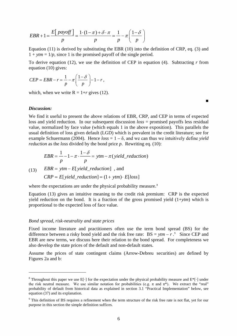
Equation (11) is derived by substituting the EBR (10) into the definition of CRP, eq. (3) and 1 + ytm = 1/p, since 1 is the promised payoff of the single period.

To derive equation (12), we use the definition of CEP in equation (4). Subtracting r from equation (10) gives:

1 1 1CEP EBR r rp p

δπ −= − = − − −

,

which, when we write R = 1+r gives (12).

■

Discussion: We find it useful to present the above relations of EBR, CRP, and CEP in terms of expected loss and yield reduction. In our subsequent discussion loss = promised payoffs less residual value, normalized by face value (which equals 1 in the above exposition). This parallels the usual definition of loss given default (LGD) which is prevalent in the credit literature; see for example Schuermann (2004). Hence loss = 1 – δ, and we can thus we intuitively define yield reduction as the loss divided by the bond price p. Rewriting eq. (10):

(13)

1 11 ( _ )

[ _ ] , and[ _ ] (1 ) [ ]

EBR ytm yield reductionp p

EBR ytm E yield reductionCRP E yield reduction ytm E loss

δπ π

−= − − ⋅ = −

= −

= = + ⋅

where the expectations are under the physical probability measure.8

Equation (13) gives an intuitive meaning to the credit risk premium: CRP is the expected yield reduction on the bond. It is a fraction of the gross promised yield (1+ytm) which is proportional to the expected loss of face value.

Bond spread, risk-neutrality and state prices Fixed income literature and practitioners often use the term bond spread (BS) for the difference between a risky bond yield and the risk free rate: BS = ytm – r .9 Since CEP and EBR are new terms, we discuss here their relation to the bond spread. For completeness we also develop the state prices of the default and non-default states.

Assume the prices of state contingent claims (Arrow-Debreu securities) are defined by Figures 2a and b:

8 Throughout this paper we use E[·] for the expectation under the physical probability measure and E*[·] under the risk neutral measure. We use similar notation for probabilities (e.g. π and π*). We extract the “real” probability of default from historical data as explained in section 3.1 “Practical Implementation” below, see equation (37) and its explanation. 9 This definition of BS requires a refinement when the term structure of the risk free rate is not flat, yet for our purpose in this section the simple definition suffices.

7

[INSERT FIGURE 2a,b]

The law of one price requires:

(14) 1

u dq qR= + and u dp q qδ= + ⋅

From the prices of these two traded securities we can easily calculate the state prices:

(15) / 1 1/,1 1u d u

p R R pq q qR

δδ δ

− −= = − =

− −

The state prices are positive and well defined when 1/p > R > δ/p and δ < 1. The risk neutral probability of a “down” state is given by:

(16) 1 1 /

*1 1 / /d

p R p R u Rq R

p p u dπ

δ δ− ⋅ − −

= ⋅ = = =− − −

,

where: u = 1/p and d = δ/p are the “up” and “down” gross returns of the risky bond.10 Rearranging the above and using the definitions of BS and yield reduction :

(17) 1(1 )

*_p

ytm R BS

yield reductionδπ

−

+ −= =

hence

(18) [ ]*BS E yield reduction= ,

where E* denotes expectations under the risk-neutral measure. Comparing BS with CRP, we see that both are expected values of the yield reduction, under the risk-neutral and physical probabilities respectively:

(19) [ ] [ ] ( )( )* * 1 /BS CRP E yield reduction E yield reduction pπ π δ− = − = − −

Rearranging (12) and using our definition of expected yield reduction (13):

1 1 1[ _ ]CEP R R E yield reduction

p p p

δπ

−= − − ⋅ = − −

1/p – R is the bond spread (by definition) and equals the risk-neutral expected yield reduction by (18). Therefore:

(20a) [ _ ] [ _ ]CEP E yield reduction E yield reduction∗= −

and

(20b) CEP BS CRP= −

It is also easy to show that:

10 These results and definitions are identical to those of binomial trees used in option pricing where d < R < u , otherwise admitting arbitrage opportunities. Thus π* and 1- π* are non-negative and smaller than 1, forming the RN probability set which is defined uniquely by the market price of the risky zero-coupon bond, its recovery rate and the market risk-free rate for the period.

8

(21) 1 1 ( )(1 )

1 (1 )CEP R R

p p

δ π π δπ

π δ

∗

∗

− − −= − ⋅ − =

− −

This result shows clearly that CEP which embodies the risk aversion premium is monotonically increasing with the difference between the risk neutral and the physical probabilities of default. It is also directly (though not linearly) related to the relative loss given default (1-δ) on the bond.

Multiple Period Tree Model We now show that the results of the previous sub-section can be extended to a multi-period framework. There is a vast volume of research and publications on tree models for bond pricing. We mention just a few of them. Black, Derman, and Toy (1990) impose a structure of a risk free interest tree based on market observed prices and volatilities. Jarrow and Turnbull (1995) focus on the default process and its integration into an interest rate (bond price) tree. Broadie and Kaya (2007) construct a binomial tree that can incorporate various “real-life” features, yet it is actually a versatile and practical implementation of structural models whereas our model is of the reduced-form type.

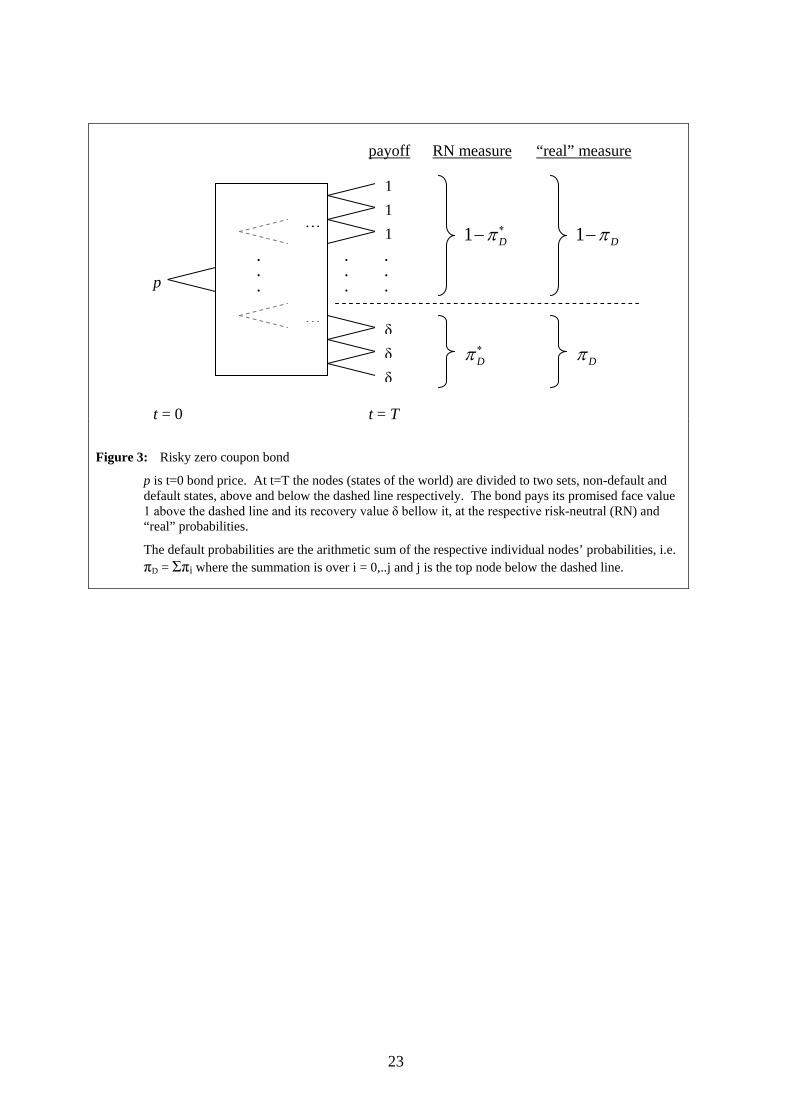
Consider a zero coupon bond which can default at maturity.11 Figure 3 describes a zero coupon risky bond that pays the promised face value 1 if it does not default and its recovery value δ if it defaults. We assume here that the bond value upon default is a constant δ representing the recovery percentage. What makes this model attractive and tractable is its simplicity. It divides the world into two major states: the nodes above the dashed line and the nodes below it (in Figure 3). The states above the dashed line are no-default states, and since they have identical payoffs their probabilities can be added when calculating expectations under the RN or real measure. The same rationale applies to the default nodes below the line. Thus we do not need to know the probability of an individual node to calculate the expected payoff at bond maturity. It suffices to know that the bond defaults at a probability πD and does not default at a probability 1- πD.

[INSERT FIGURE 3]

The same tree is relevant for the case where default might occur prior to T and the recovery is adjusted to the money market at T.12 We also assume that the (gross) risk-free interest rate for the period t=0 to t=T is RT.

Theorem 2: Consider a T-period zero-coupon bond. Denote the probability of default at time T by πD, the bond price by p, the recovery rate by δ, and the current one-period gross (i.e., one plus) interest rate by R1.13 Then the following relations hold:

11 We briefly explain later when and how this assumption can be relaxed and adapted to allow default at any time. 12 This is known as the “Recovery of Treasury” model, where bondholders recover a fraction of the present value of face. For this definition and others including further references see for example Uhrig-Homburg, M., 2002, “Valuation of defaultable claims: A survey,” Schmalenbach Business Review, 54, 24-57. This discussion is beyond the scope of this paper. To analyze such a case we need additional assumptions that we avoid in our present model and to be prudent about the probability measure (for applying this model to default before maturity T).

9

• The expected bond return is given by:

(22) ( )

1/1 1

1

T

DEBRp

π δ− −= −

• The credit risk premium is given by:

(23) ( ) 1/

1/

1 1 1D

T

TpCRP ytm EBR

π δ− − −= − =

• The certainty equivalent premium is given by:

(24) ( )

1/

1

1 1T

DCEP Rp

π δ− −= −

Proof: Equation (22) follows directly from the definition of EBR and the setup of Figure 3:

( ) ( )1/ 1/

1 1 1 11 1

T T

D D DEBRp p

π δ π π δ⋅ + − ⋅ − −= − = −

To derive (23) we required an expression for ytm which by its definition is given by:

(25)

1/1

1T

ytmp

= −

Using (22) and (25) and the definition of CRP results in equation (23):

( )[ ] ( )[ ]1/1/ 1/

1/

1 1 1 1 11TT

D D

T

TCRP ytm EBR

p p p

π δ π δ− − − − −= − = − =

.

Equation (24) then follows directly from the relation of EBR and the risk-free rate in a frictionless world:

( )1/

1 1

1 11

T

DCEP EBR r EBR R Rp

π δ− −= − = + − = −

■

The above and subsequent relations hold for the general case, where the term structures are not flat. Each return and premium value is a function of the maturity T which is omitted in our expressions for ease of notation.

13 In the prior section we use R for the single period gross risk free rate for single period model. Here we use R1 in the multiperiod model to avoid confusion with RT. Actually R1 = (RT)1/T. Thus when the term structure is not flat R1 ≠ R = a one period ahead rate.

10

Discussion: We start with the bond price using risk-neutral pricing:

(26) ( )

( )

* *

*

1 1

1 1

D D T

D T

p

p

R

R

δ

δ

π π

π

= ⋅ + − ⋅

= − −

Hence p = PV{1 – E*[loss]} for a unit face value, where PV is the present value using the risk-free rate and E* denotes the expected value under the RN probabilities.

The economic meaning of the nominator of (22) is simply {1 – E[loss]}, where E denotes the expected value under the “real” probabilities. Hence the gross EBR ( = 1+ EBR) of a zero coupon bond has an intuitive meaning of a per-period expected gross return on the initial investment (the time 0 price of the risky bond) and it is linearly related to the gross risk-free rate:

(27) ( ) { } ( )1 [ ] 1 [ ] 1 [ ]1

1 [ ] 1 [ ]1T TE loss E loss E loss

EBRp PV E loss E loss

r∗ ∗

− − −+ = =

− −= ⋅ +

The single period credit risk premium (CRP) is the fraction of the gross promised yield (1+ytm) which is proportional to the expected loss of face value, see equation (13). The multi-period expression in (23) is the "per period" equivalent of (13) and has similar interpretation.14

Equation (24) for the certainty equivalence premium can be rewritten, translating its components to yields and expected loss:

(28) ( )1/

11 [ ] (1 )TCEP E loss ytm R= − + − .

Equation (28) shows that a risk averse investor requires a premium over the risk free rate which is linearly related to the product of the gross promised return and the “per period” expected payoff. Again the expectations are with regards to the “real” probabilities and the payoffs are rates since they are normalized by the face value of the bond (which is 1 in our case). This can be interpreted as if the investors expect that promised returns (1+ytm) will not be fully realized. They expect that only a fraction will be actually gained. This fraction is embodied in (1-E[loss]). When T increases. this factor grows (for a constant E[loss]) and increases CEP for the same promised returns.15

To conclude, it can be easily shown that the bond-spread decomposition of equation (20a, b), of the single period tree, which states that BS is the arithmetic sum of CRP and CEP, holds in our multiple period “black box” tree model for zero coupon bonds. That is, in a frictionless world:

14 Using the relation (25) between 1+ytm and 1/p. The expression in the square brackets equals the expected payoffs at T, thus its Tth root can be viewed (intuitively) as the per-period expected payoff and its difference from 1 is the per period expected loss value. 15 As T grows substantially, ceteris paribus, this fraction approaches 1. This result is obviously extreme and irrelevant since E[loss] also increases with T and thus the above sensitivity analysis should serve our intuition only for relatively small changes in the parameters. Furthermore, the model of (24) and (28) of zero coupon bond does not hold for unbounded maturity. The default probability approaches 1 and the price of a very distant future, highly risky payment of $1 (that would materialize at a miniscule probability), approaches zero as T increases.

11

ytm = r + CRP + CEP

Intuitive interpretation Additional insight can be gained by writing the multi-period expressions of Theorem 2 in a form that approximates the one-period expressions of Theorem 1. The general binomial theorem (see Appendix C) gives the following approximation:

(29) ( ) ( )1/ 1

1 1 1 1D D

T

Tπ δ π δ− − ≈ − −

The Tth root of a bond price (equation 26) can be approximated by the present value (discounting at one-plus the one-period risk free rate R1) the face value less "average single period" expected loss (expectations under risk-neutral probability).

(30) 1/1/ * *

1 1

1 1 11 (1 ) 1 (1 )

TT

D DpR R T

π δ π δ= − − ≈ − −

Substituting the same binomial approximation in EBR and CRP results in:

(31) 1

1*1

1 (1 )1

1 (1 )DT

DT

EBR Rπ δ

π δ

− −≈ −

− −

(32) 1

1*1

(1 )1 (1 )

T D

T D

CRP Rπ δπ δ

−≈

− − .

When the second term, the risk-neutral expected per-period loss rate, in the denominator of (32) is sufficiently small, then CRP is approximately linear in the expected per-period loss rate. In the general case, the relation is not linear and CRP grows monotonically with the expected per-period loss rate, as can be seen in (32b):

(32b)

1 1

1 1* *1 1 1

1

11

(1 ) (1 )1 (1 ) 1 (1 ) (1 )

(1 )1 (1 ) (1 )

( )

/

T TD D

T T TD D D D

T D

T D

CRP R R

RCEP ytm

π δ π δπ δ π δ π π δ

π δπ δ

− −≈

− − − − − −

−− − − +

= =−

=

where the last term in the denominator follows from (34). Another interesting expression results from rearranging (32):

(33) ( )1

1* 1/1

(1 ) [ ] / [ ] 11 (1 )

DTT

DT

E loss T E lossCRP R ytmp T

π δπ δ

−≈ = = +

− −

Where the loss in this expression is actually a loss-rate since it is a fraction of $1 face value. Equation (33) is the T-period equivalent of the single period expression (13).

Expression (31) shows that EBR is the risk-free rate when the physical measure equals the risk-neutral measure. This agrees with our earlier discussion of risk neutral investors, requiring just a risk free rate in a frictionless world. When the recovery is complete (δ=1)

12

there is no risk and again EBR = risk free rate. Otherwise EBR+1 is R1 multiplied by the ratio of the per-period expected residual values where the physical expectation is divided by the risk neutral one.

Using (31) to approximate EBR in (4), we find (34), which shows how the risk aversion expressed by the CEP is related to the difference between the risk-neutral and physical probabilities of default, the per-period average loss, and the gross required yield ( = 1+ ytm which equals Rf divided by the denominator of (34), as can be seen above).

1

1 1*1

1 (1 )1 1

1 (1 )T D

T D

CEP EBR r EBR R Rπ δπ δ

− −= − = + − ≈ −

− −

(34)

( )1

1 1

(1 )

1 (1 )T D D

T D

CEP Rδ π π

π δ

∗

∗

− −≈

− −

3. Empirical results We present below practical estimation method and empirical results of Section 2 model and relations.

3.1 Practical Implementation We discuss below three implementation matters: extracting the zero-coupon term structure of interest rates (TSIR), the “real” probability of default term structure, and selecting a proxy for the risk free rate.

Zero coupon term structure of interest rates estimation Fitting a “best” term structure to the noisy numerical data of interest rate has been discussed by many researchers and practitioners. Subramanian (2001) describes the main functional forms that have been used in the literature: polynomial, exponential and B-splines, exponential polynomial forms for the forward rate, and roughness penalty methods. These and additional methods are discussed by Hagan and West (2006) who also offer additional insights and interpolation procedures for hedging applications.

We use Nelson and Siegel (NS) (1987) model for the representation and interpolation of our results. This method is often the procedure of choice by practitioners and was found superior to alternative methods by Subramanian (2001) and others.16 NS parameters can be linked to common factors affecting bond returns, namely level, steepness, and curvature of Litterman and Scheinkman (1991). They found that these three factors explain on average more than 98% of the variations in bond returns. The percentages change with bond maturity and on average level, steepness, and curvature account for 89.5%, 8.5%, and 2% of the variations respectively. Similar results are confirmed for later periods, Ramaswamy (2004) for example, shows similar results by principal components analysis on 1999-2002 data set (pp. 58-59).

16 S&P proposal (dated 19 Feb 2004) to the Israeli government (tender 8/2003) for modelling and provision of term structures of interest rate for national mutual funds, provident funds, and insurance companies.

13

NS 1987 was also scrutinized for allowing arbitrage, e.g. Bjork and Christensen (1999). Coroneo et al (2008) investigated this matter statistically and concluded that the Nelson and Siegel yield curve model is compatible with arbitrage-freeness.

For the sake of completeness we repeat NS model below:

(35) ( ) ( ) ( )0 1 2 2

1 exp /( ) exp /

/m

r m mm

τβ β β β τ

τ− −

= + + ⋅ − ⋅ −

Where:

m is the time variable

β0 and (β0+β1) are the long-term and short-term rates respectively

τ is a parameter that specifies the position of the hump

β2 is the medium term component which determines the magnitude and the direction (up or down) of the hump or trough in the yield curve.

We need to estimate a term structure of interest rate (TSIR) for each rating category. This poses two issues:

a) An unconstrained NS curve fit often results in TSIR curve crossing, i.e. a higher rating might have a higher return than a lower rating at certain maturity ranges. This obviously has no reasonable economic support and is regarded as an undesirable artifact of the NS curve fit and data noise. A practical remedy to this issue is using a constrained NS curve fit as follows:17

• Allow only monotonic non-decreasing term structure (monotonicity).

• At any maturity the lower rating TSIR should be no lower than the next higher rating TSIR (no-crossing).

• Start the curve fit with the highest rating (AAA in our case) adhering to the monotonicity requirement only. Then, one at a time, move to the nearest lower rating requiring both monotonicity and no-crossing.

b) Preferably, the curve fit is a daily one, based on a single day rich transaction data, for each day of our sample. Our data however is scattered over a period of four months. We have thus chosen to use a TSIR representative of the four month period, a single curve for each rating category. All curves are referenced to the same day (see details below). We are not aware of others that have adopted the same mechanism, yet under the assumptions of time invariant TSIR for the data period of four months we believe our methodology is theoretically sound.

For the curve fit we use the constrained optimization function of MatLab (fmincon). The goal is to minimize the error function which is the sum of the absolute pricing errors of all the transaction quotes of the specific rating during the data period. The pricing error of a bond is its market (quoted) dirty price less its calculated price based on the TISR given by the estimated NS curve. For consistency the market and calculated prices are discounted to the reference date of the NS curve (1 Sep. 2004 in our case). We tried minimizing sum of squared pricing errors and selected the sum of absolute errors to avoid emphasizing the effect of outliers in our noisy data. 17 This method is widely adopted by S&P and was implemented in “Shaarey Ribit” the national standard in Israel for the TSIR of government and corporate bonds (as of 2004).

14

Term structure of “real” default probability We use the commonly accepted (de facto) “standard” of rating transition matrices, published by the rating agencies, to estimate the physical default probability. We generate a series of the time t state vector st:

(36) 0t

ts s′ ′= ⋅Π

where the ith component of st is the probability that the bond is in state (rating), i = 1,…N, and where s’ is the transpose of vector s. The πi,j element of the transition matrix Π is the probability that a bond which has a rating i at the beginning of the period t would have the rating j at its end. Hence:

(36a) 1 1,...t ts s t T−′ ′= ⋅Π ∀ =

assuming a time invariant Π, where T is the maturity of the bond. Since st is a vector of probabilities assigned to exclusive states (ratings) at time t, ι’· st = 1, where ι is the vector of ones. We define the states 1,.., N-2 to be the solvent ratings (AAA,…, C for the case of S&P ratings), the N-1 state is a default state (for a default event at time τ = t) and the Nth state is a post default state (where default occurred in the past, at time τ < t). The above definitions and process lead to a simple calculation of the “real” probability of default (πD) at the end of any time period t:

(37) πD,t = st,N-1 + st,N

where N-1 and N subscripts denote the last two elements of the state vector st.

Risk free rate The US government bond TSIR is often used as a benchmark risk free rate. We do not propose a better benchmark. However, we need to control for the effects of liquidity premium and taxes to improve our estimates of the risk-neutral default probability term structure. Afik-Benninga (AB, 2010) demonstrate that the credit premium and real default probabilities are almost negligible for AAA rated bonds, yet they command a significant “other” premia above the treasury TSIR. Thus, we adopt the AAA TSIR as our risk-free benchmark, assuming it nets out (at least partially) the liquidity and tax effects of the other ratings.

We acknowledge that there are liquidity differences among the various ratings and that taxes may affect differently speculative bonds and investment grade ones, yet we ignore these secondary effects in our current research.

3.2. Sample results and discussion The following describes and discusses our results of estimating the above yields, premia, and default probability measures for a dataset of US corporate bonds transactions.

15

The data A complete and reliable corporate bond data remains one of the challenges in our research. For the current research we use The Fixed Income Securities Database (FISD) for academia on Wharton’s site. It covers over 100,000 corporate, U.S. Agency, U.S. Treasury and supranational debt securities and includes more than 400 fields or data items. FISD might be biased to bond portfolio activity of insurance companies including infrequent trading, biased to initial offer, large volumes, long term holding periods, and other specific sample and price biases. The Wharton database is a subset of FISD database intended for academic research. Amongst its drawbacks is the absence of recent data. We processed and analyzed the transactions of a four month period spanning September to December 2004. At the time of our analysis the coupon payment frequency was not included in the Wharton database and we used a private database to complete our data set (identifying the individual bonds by their ISIN codes).

We used only corporate bonds that pay fixed coupons semiannually. All other were excluded from our data set. We also excluded other data including:

• Bonds not rated by S&P

• Callable, putable, and convertible bonds

• Bonds with less than 3 coupons remaining and longer than 40 years to maturity. (Thus including 1 < maturities ≤ 40 years in our data set.)

• Transaction data without a price quotation (or non positive price)

• Bonds for which we failed matching a complete set of inputs required for our calculations.

Our initial raw data includes 115,507 transaction lines. After filtering and fusion of data from other tables we have 11,209 transaction lines with complete data sets for our analysis. Filtering these transactions of US government agencies bonds results in a net of 6,445 transactions that are usable for our calculations.18 The statistics of the net final set are presented in Appendix D.

We looked at S&P500 as a proxy for the equity market behavior during our sampled period. We believe it shows that it has been typically a steady and relatively uneventful period compared to the two year preceding the sampled period and the two years that have followed it. Since it is widely accepted that the corporate bond market is strongly linked with the equity market performance, empirically, and explained by various structural models, we cannot rule out that our bond data results are typical of a steady growing market without outstanding booms and without significant crashes.

Results examples and discussion

Zero-coupon bond term structure of returns First we estimate the TSIR of the S&P rating categories for our data set.

18 The 4,764 US government related bonds filtered in the last stage do not represent their relative size in the total transaction number. These are just the residual that were not filtered earlier in the query of the FISD database. They were filtered out by their CUSIP (after noticing their outstanding results compared to the bulk of corporate bonds).

16

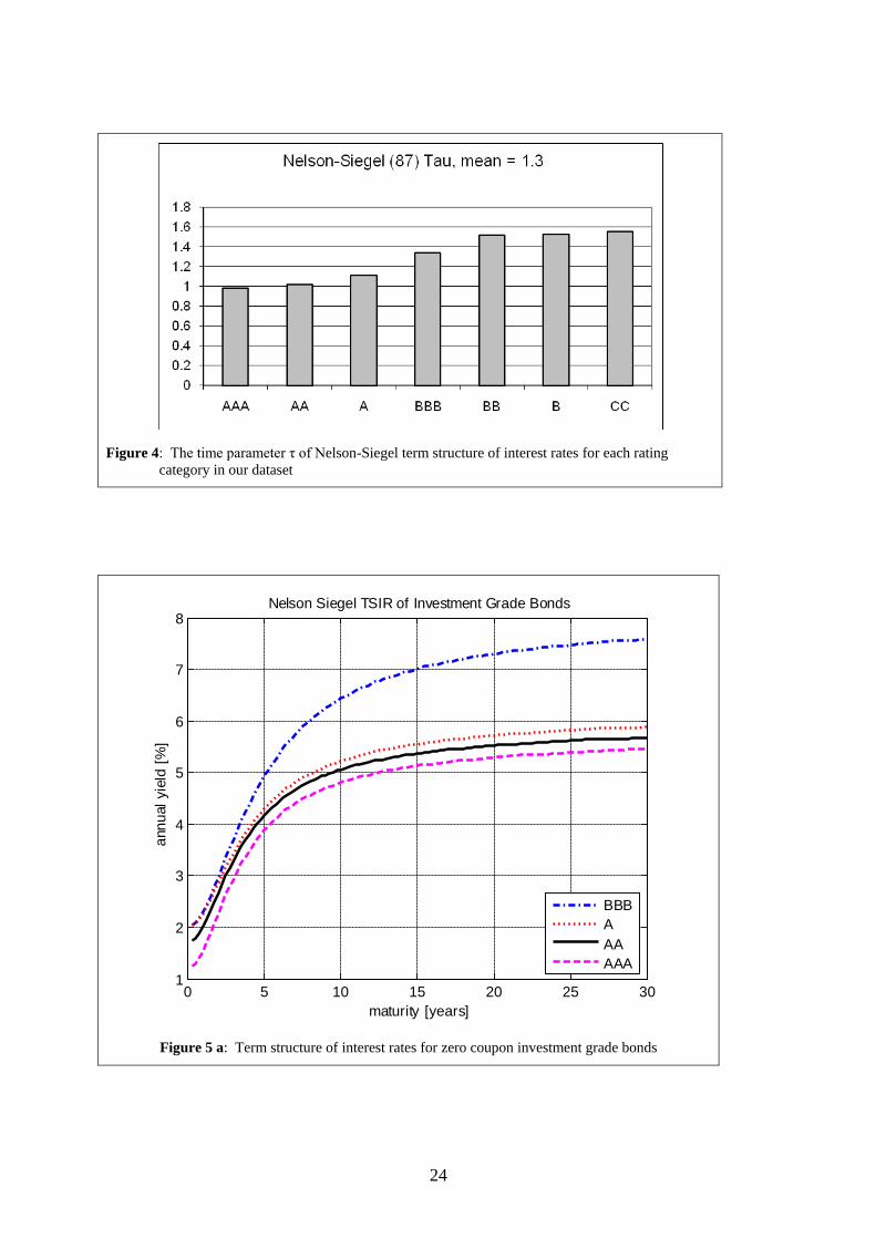
As explained above, for each rating we estimate the four NS parameters defining the rating TSIR. To avoid undesirable crossing of fitted curves we impose certain constrains in our estimation process as explained above,. Others, such as Diebold and Li (2006) have chosen to estimate a linear model of NS β0÷β2 parameters and imposed a constraint on the fourth (non-linear) parameter τ = 1.3684.19 This value is not remote from our results, see Table 1 and Figure 4, yet we do not see a reason to impose this constraint in our case.

[INSERT FIGURE 4]

[INSERT TABLE 1]

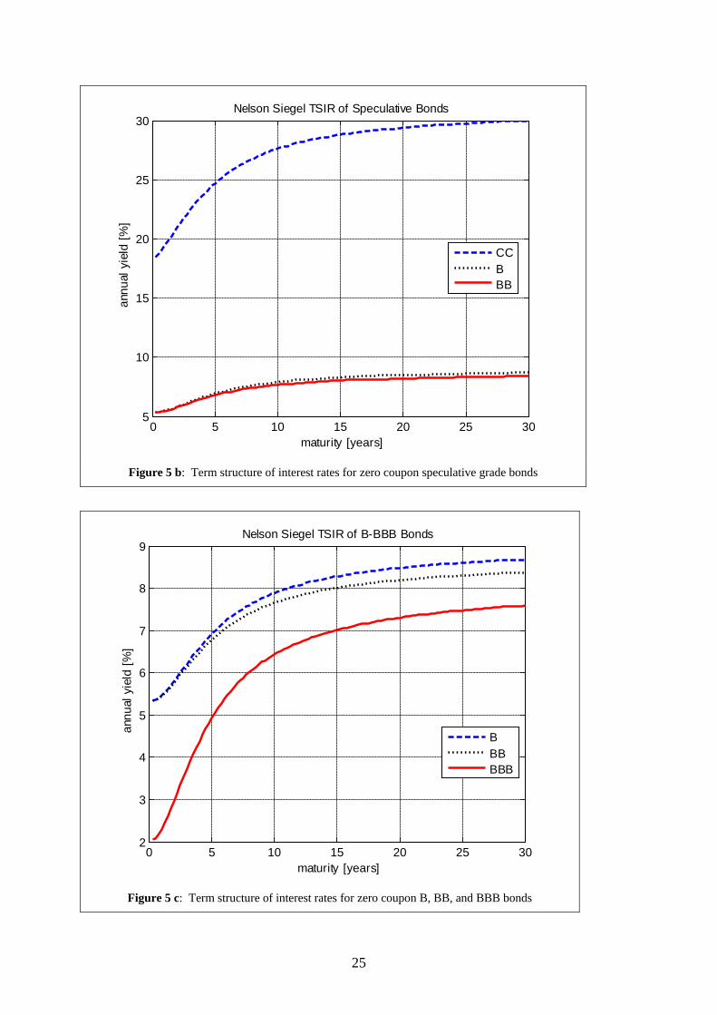
Remembering that β0 and (β0+β1) are the long-term and short-term rates respectively, the results of Table 1 seem economically reasonable. Figures 5a and 5b show the TSIR of our NS fit for zero coupon bonds extracted from our data for investment and speculative grade respectively. Figure 5b shows that the C-CCC graded bonds actually form a separate class in our data set. We therefore added Figure 5c that depicts more clearly the B-BBB TSIR’s. These figures show that in our dataset there is a distinct clustering of the TSIR’s to the three major rating categories A, B, and C, with pronounced spreads between them compared to the intra-group spreads.

[INSERT FIGURE 5a,b,c]

Default probabilities term structure We compute πD “real” probabilities as explained in section 3.1 above using S&P transition matrix (see Appendix B). For the calculations of risk-neutral (RN) default probabilities πD* we use equation (26). It expresses the relation among the transaction price p, observed in the market, the risk free rate RT, which we assume is proxied by the AAA TSIR, the recovery rate δ, which we assume equals 40% for all ratings, and the estimated πD*. More robust estimation is proposed for the RN expected loss: E*[loss] = πD*·(1- δ), which does not require an assumed recovery rate.

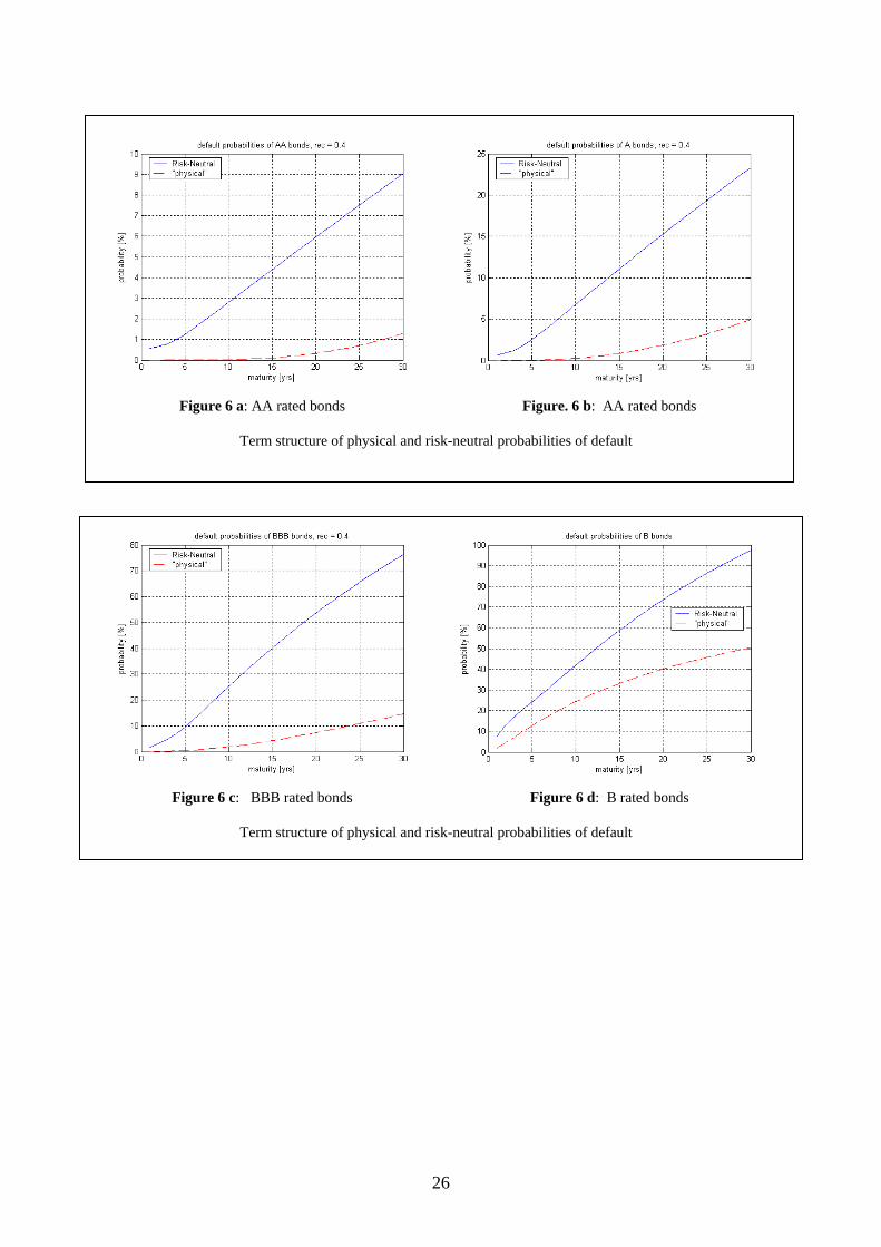
Figures 6a-d show a sample of “real” and RN default probabilities of AA, A, BBB, and B bonds. The results for BB bonds are intermediate between those of BBB and B bonds. The results for C bonds are based on a small sample, 16 transactions only, and thus are unreliable (especially in comparison to the other rating samples).

[INSERT FIGURE 6a,b,c,d]

These results are in agreement with results obtained by Delianedis and Geseke (2003) who compute risk-neutral default probabilities using the option-pricing based models of Merton (1974) and Geske (1977). They show, not surprisingly, that their estimates for the risk-neutral default probabilities from both models exceed rating-migrations based physical default probabilities.

[INSERT FIGURE 7]

[INSERT FIGURE 8a,b,c,d]

Bond yield decomposition Using the above estimated zero-coupon returns and default probability term structures of each of the rating categories, we estimate the expected bond returns (EBR), the credit risk 19 Diebold and Li (2006) quote an inverse value on a monthly basis (p. 347), λ = 0.0609. Since we use the original parameter τ of the NS model on annualized time periods this number is inverted and multiplied by 12.

17

premium (CRP) and the certainty equivalence premium (CEP) term structures using equations (22), (23), and (24) respectively.

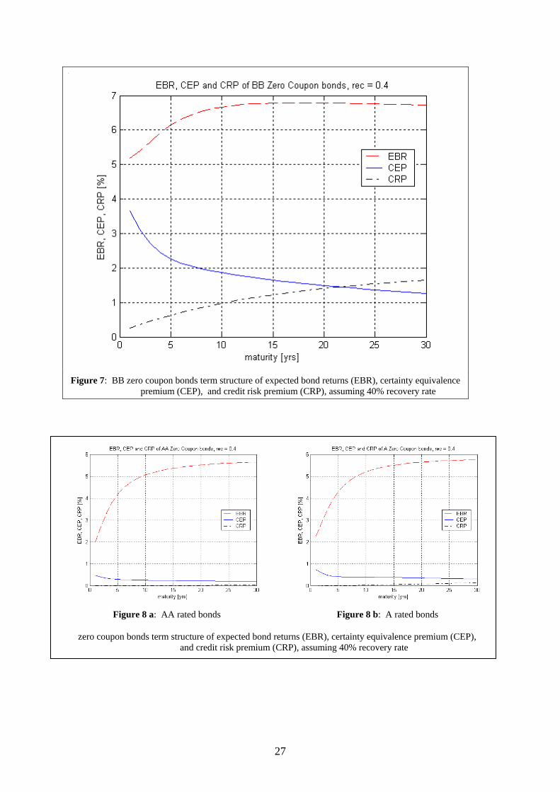
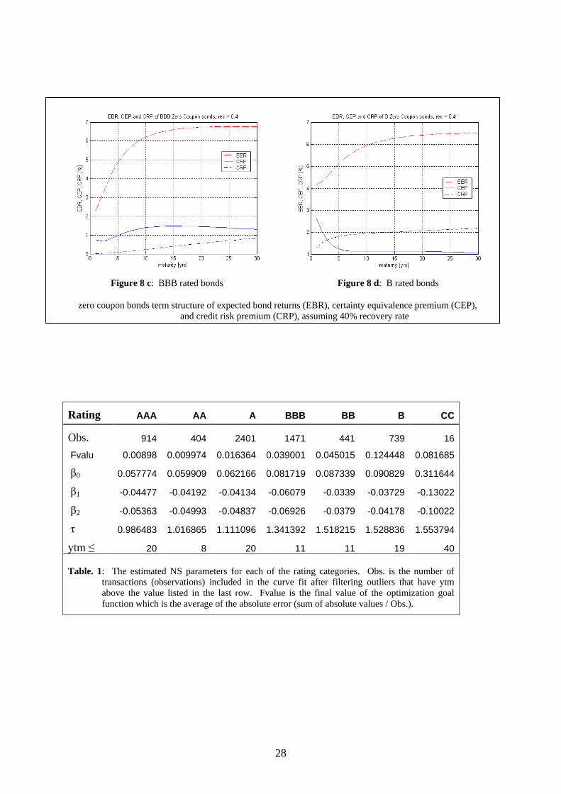
Figure 7 shows the term-structures of EBR, CEP, and CRP of zero coupon bonds rated BB. Figures 8a-d show similar charts for ratings AA, A, BBB, and B respectively.

It is worthwhile recalling that (1+EBR)T = (1 – E[loss])/p = (1+ytm)T - E[loss])/p where the expectations are under the “real” probability measure. CRP is the difference between ytm and EBR and thus expresses a per-period related expected loss rate (of the promised gross yield 1+ytm), see the approximation in equation (33). The CEP in a frictionless world is the difference between EBR and the risk-free rate. In our estimation we assume that the market friction premia (mainly liquidity, transaction cost, bid-ask, and tax effects) are embodied in AAA rated zero coupon bond returns. Thus we estimate CEP of rating j bonds by:

CEPj(T) = EBRj(T) – ytmAAA(T) for each maturity T.

EBR increases monotonically with declining bond rating, and usually with maturity (except for BB bonds that exhibit a slowly decreasing term structure at long maturities). While CRP monotonically increases with maturity and with decreasing bond rating, CEP generally decreases with maturity, exhibiting a humped shape for BBB rated bonds. CEP increases with decreasing bond rating for investment grade bonds. There is no clear order for CEP of speculative graded bonds. Since the CEP expresses the risk aversion to the lottery, the additional discount investors demand of EBR above the risk-free rate, it seems that the perceived “lottery” risk is not significantly magnified by the decreasing rating. We postulate that this happens because the investors are compensated by a significantly higher CRP for lower grade bonds.

It is worth mentioning that CEP is related to the CAPM “systematic risk”. This relation is presented in Appendix A. The above finding that CEP does not vary materially among speculative graded bonds is maybe an evidence that their risk differences are not materially related by market participants to systematic risk differences.

4. Conclusions and Further Research Directions We developed a simple, intuitive, and practical framework for modeling and estimating the term structure of zero-coupon expected bond returns and the decomposition of bond yields.

We estimated these yields and premia using US corporate straight-coupon-bond market data of the period September-December 2004. As a by-product of this process we also estimated a term structure of default probabilities for each bond rating under the risk neutral and the “physical” measures.

This paper extends a single period tree into a multiple period “black box” tree, avoiding the structural assumptions often required for “open box” trees. This is possible since we focus mainly on zero coupon returns and spreads. Despite its simplicity, this approach also enables better understanding of EBR and its components. Our model avoids a specific structure and assumptions regarding the process dynamics (of state variables) and the relation among the parameters of the inner nodes of the tree. Yet this is done “at the cost” of remaining more abstract - the interim periods prior to maturity remain a blackbox. We also impose, similar to many other models, a fixed recovery rate upon default.

Since we estimate the expected bond returns (EBR), the credit risk premium (CRP), and the certainty equivalence premium (CEP) from market prices and the information set available to the investor, EBR, CRP, and CEP are implied by the market information and may change as a

18

result of market prices for example. We do not regard such dependence on prices as a weakness. On the contrary, assuming market prices embody the collective expectations of future payoffs, our model “calibrates” the ex-ante term structures of EBR, CRP, CEP, and risk-neutral default probabilities to these expectations.

Our model also bridges the gap between the literature of equities and bonds. By defining the CRP and calculating EBR the two literatures are comparable in terms of expected returns. Additionally, CAPM systematic risk has been adopted mainly for equities. The CEP term structure provides a forward looking, ex-ante implied systematic credit risk of bonds (for each rating category). The clear breakdown of bond spread to CRP, CEP, and other premia (the sum of liquidity, tax, transaction cost, etc.) helps clarify and estimate the components of this important and useful spread.

Jarrow, Lando, and Turnbull (JLT) (1997), and follow on works, estimate a risk-neutral set of transition matrices based on the "physical" measure transition matrix of a rating agency and bond market data. Their estimation assumes certain structure and relations between the risk-neutral and the "physical" matrices. We avoid these assumptions and we estimate the risk-neutral default probability term structure of various rating groups directly from the zero coupon term structure of interest rates of the relevant rating groups. We estimate the required term structures from bond market data. Though our method does not estimate a complete risk-neural set of transition matrices, we believe our model is more robust, less noisy, and requires lesser assumptions than JLT.

Coupon bond EBR and CRP estimation follow the definition of equations (2) and (3). The details of the estimation process and examples from the US corporate bond market are beyond the scope of this paper.20

We have focused our work on developing the model and the empirical estimation process. Therefore our empirical results are limited to a relatively short period. We plan on expanding our data set and explore the model results on additional periods. We also believe that this paper model provide a basis for further research and applications such as implied recovery and implied rating, which will be presented in subsequent papers.

We demonstrated the estimation using unconditional rating transition matrices. A similar estimation seems feasible using conditional default probabilities that can be estimated using hazard models. We believe that these open new opportunities for researchers and practitioners.

20 These are included in a separate, currently a working paper whose earlier draft Afik and Benninga (2010) is available on SSRN.

19

References Afik, Z., and S. Benninga, 2010. “Expected Bond Returns: a Markov model and market

data.” Working paper (available on SSRN, No. 1564001).

Altman, E.I. and Allan C. Eberhart, 1994. “Do Seniority Provisions Protect Bondholders’ Investments?” Journal of Portfolio Management, Vol 20, no 4 (Summer): 67-65.

Altman, E., and V.M. Kishore, 1996. “Almost Everything You Wanted to Know about Recoveries on Defaulted Bonds,” Financial Analysts Journal, (November/December): 57-64.

Bahar R. and K. Nagpal, 2001. “Dynamics of Rating Transition”, Algo Research Quarterly, 4 (Mar/Jun), Pages 71-92.

Bakshi G., D.B. Madan, and F.X. Zhang, 2004. “Understanding the Role of Recovery in Default Risk Models: Empirical Comparisons and Implied Recovery Rates,” EFA 2004 Maastricht Meetings Paper No. 3584; AFA 2004 San Diego Meetings; FEDS Working Paper No. 2001-37.

Bjork, T., and B.J. Christensen, 1999. "Interest Rate Dynamics and Consistent Forward Rate Curves." Mathematical Finance 9, 323–348.

Black, F., E. Derman, W. Toy 1990. “A One-Factor Model of Interest Rates and Its Application to Treasury Bond Options.” Financial Analysts Journal (Jan/Feb), 46, 1.

Broadie, M. and O. Kaya, 2007. “A Binomial Lattice Method for Pricing Corporate Debt and Modeling Chapter 11.” Journal of Financial and Quantitative Analysis (Jun), 42, 2.

Campello, M., L. Chen, and L. Zhang, 2008. “Expected returns, yield spreads, and asset pricing tests.” Review of Financial Studies, 21(3), 1297-1338.

Cantor, R., D.T. Hamilton, and J. Tennat, 2007. "Confidence Intervals for Corporate Default Rates." SSRN.

Coroneo, L., K. Nyholm, and R. Vidova-Koleva, 2008. "How Arbitrage-Free is the Nelson-Siegel Model." Working Paper No. 874 (February), European Central Bank.

Delianedis, G. and R.L. Geske, 2003. "Credit risk and risk neutral default probabilities: information about rating migrations and defaults." UCLA Working Paper.

Diebold, F. X. and C. Li, 2006. “Forecasting the Term Structure of Government Bond Yields.” Journal of Econometrics, 130, 337-364.

Elton, E. J., 1999. “Expected return, realized return, and asset pricing tests.” Journal of Finance, 54: 1199-1220.

Elton, E.J., M.J. Gruber, D. Agrawal, and C. Mann, 2001. "Explaining the rate spread on corporate bonds." Journal of Finance, Vol. 56, No. 10, 247-277.

Fama, E. and K.R. French, 1993. “Common risk factors in the returns of stocks and bonds.” Journal of Financial Economics, 33, 3–56.

Gebhardt W.R., S. Hvidkjaer, and B. Swaminathan, 2003. “The Cross-Section of Expected Corporate Bond Returns: Betas or Characteristics?” SSRN

Geske, R., 1977. "The Valuation of Corporate Liabilities as Compound Options." Journal of Financial and Quantitative Analysis, 541-552

20

Hagan, P., and G. West, 2006. “Interpolation methods for yield curve construction.” Applied Mathematical Finance, Vol. 13, No. 2, 89–129

Hanson, S., and T. Schuermann, 2006. "Confidence intervals for probabilities of default." Journal of Banking & Finance, 30, 2281–2301

Israel, R.B., J.S. Rosenthal, and J.Z.Wei, 2001. "Finding Generators for Markov Chains via Empirical Transition Matrices with Applications to Credit Ratings." Mathematical Finance, (April), 245-265.

Jafry, Y. and T. Schuermann, 2003. “Metrics for Comparing Credit Migration Matrices,” Wharton Financial Institutions Working Paper #03-08.

Jafry, Y. and T. Schuermann, 2004. "Measurement, Estimation and Comparison of Credit Migration Matrices." Journal of Banking & Finance, 28, 2603-2639.

Jarrow, R., 1978, “The relationship between yield, risk, and return of corporate bonds, Journal of Finance,” 33, 1235-1240.

Jarrow, R.A., D. Lando, and S.M. Turnbull, 1997. “A Markov model for the term structure of credit spreads” Review of Financial Studies, 10 , 481–523.

Jarrow, R.A., D. Lando, and F. Yu, 2005. “Default Risk and Diversification: Theory and Applications,” Mathematical Finance, 1, (January), 1-26

Jarrow, R.A., and S.M. Turnbull, 1995, “Pricing derivatives on financial securities subject to credit risk,” Journal of Finance, 50, 53-85.

John, K. S., A. Ravid, and N. Reisel, 1995. “Senior and Subordinated Issues, Debt Ratings and price Impact,” working paper.

Lando, D. and T. Skødeberg, 2002. "Analyzing Ratings Transitions and Rating Drift with Continuous Observations." Journal of Banking & Finance 26, 423-444.

Litterman, R. and J. Scheinkman, 1991. "Common Factors Affecting Bond Returns." Journal of Fixed Income, (June), 54-61.

Löffler, G., 2004. “An anatomy of rating through the cycle.” Journal of Banking and Finance, 28, 695-720.

Löffler G. 2005. “Avoiding the Rating Bounce: Why Rating Agencies Are Slow to React to New Information.” Journal of Economic Behavior & Organization, Vol. 56, Issue 3 (Mar), pp. 365-381.

Merton, R. 1974. “On the Pricing of Corporate Debt: The Risk Structure of Interest Rates.” Journal of Finance 2(2): 449-470.

Nelson, C. and Siegel, A. 1987. “Parsimonious Modeling of Yield Curves.” Journal of Business 60: 473-489.

Nickell P., Perraudin W. and Varotto S., 2000. “Stability of Rating Transitions.” Journal of Banking and Finance, 24: 203-227.

Parnes, D. 2005. “Homogeneous Markov Chain, Stochastic Economic, and Non-Homogeneous Models for Measuring Corporate Credit Risk,” working paper

Ramaswamy, S. 2004. Managing Credit Risk in Corporate Bond Portfolios - A Practitioners Guide, Wiley, New Jersey.

Schuermann, T. 2004. “What do we know about loss-given-default,” Wharton Financial Institutions Center Working Paper #04-01.

21

Schuermann, T. 2007. "Credit Migration Matrices," Risk-Encyclopedia.

Schuermann, T. and Y. Jafry, 2003. “Measurement and Estimation of Credit Migration Matrices,” Wharton Financial Institutions Center Working Paper #03-09.

Subramanian, K.V., 2001. “Term Structure Estimation in illiquid Markets,” The Journal of Fixed Income, (June): 77-86.

Uhrig-Homburg, M., 2002, “Valuation of defaultable claims: A survey,” Schmalenbach Business Review, 54, 24-57.

Vazza, D. and D. Aurora, 2004. “S&P Quarterly Default Update & Rating Transitions.” S&P Global Fixed Income Research, (October)

Yu, F., 2002. “Modeling Expected Return on Defaultable Bonds,” Journal of Fixed Income 12(2): 69-81

22

Figures and tables

Figure 1a: A risk free bond Figure 1b: A risky bond

R is the risk free rate, p is the bond price, δ the recovery rate, and π the default probability (physical measure)

Figure 2a: security paying $1 at “up” state Figure 2b: security paying $1 at “down” state

qu and qd are the state prices of up (no default) and down (default) state respectively π* is the risk-neutral default probability

qd

0

1

1-π*

π*

qu

1

0

1-π*

π*

p

1

δ π

1-π

1

R

R

23

Figure 3: Risky zero coupon bond

p is t=0 bond price. At t=T the nodes (states of the world) are divided to two sets, non-default and default states, above and below the dashed line respectively. The bond pays its promised face value 1 above the dashed line and its recovery value δ bellow it, at the respective risk-neutral (RN) and “real” probabilities.

The default probabilities are the arithmetic sum of the respective individual nodes’ probabilities, i.e. πD = Σπi where the summation is over i = 0,..j and j is the top node below the dashed line.

.

.

.

…

…

p

1

1 1

.

.

.

.

.

.

payoff RN measure “real” measure

δ

δ

δ

1 Dπ∗− 1 Dπ−

Dπ∗

Dπ

t = T t = 0

24

Figure 4: The time parameter τ of Nelson-Siegel term structure of interest rates for each rating

category in our dataset

0 5 10 15 20 25 301

2

3

4

5

6

7

8

maturity [years]

ann

ual y

ield

[%]

Nelson Siegel TSIR of Investment Grade Bonds

BBBAAAAAA

Figure 5 a: Term structure of interest rates for zero coupon investment grade bonds

25

0 5 10 15 20 25 305

10

15

20

25

30

maturity [years]

ann

ual y

ield

[%]

Nelson Siegel TSIR of Speculative Bonds

CCBBB

Figure 5 b: Term structure of interest rates for zero coupon speculative grade bonds

0 5 10 15 20 25 302

3

4

5

6

7

8

9

maturity [years]

ann

ual y

ield

[%]

Nelson Siegel TSIR of B-BBB Bonds

BBBBBB

Figure 5 c: Term structure of interest rates for zero coupon B, BB, and BBB bonds

26

Figure 6 a: AA rated bonds Figure. 6 b: AA rated bonds

Term structure of physical and risk-neutral probabilities of default

Figure 6 c: BBB rated bonds Figure 6 d: B rated bonds

Term structure of physical and risk-neutral probabilities of default

27

Figure 7: BB zero coupon bonds term structure of expected bond returns (EBR), certainty equivalence

premium (CEP), and credit risk premium (CRP), assuming 40% recovery rate

Figure 8 a: AA rated bonds Figure 8 b: A rated bonds

zero coupon bonds term structure of expected bond returns (EBR), certainty equivalence premium (CEP), and credit risk premium (CRP), assuming 40% recovery rate

28

Figure 8 c: BBB rated bonds Figure 8 d: B rated bonds

zero coupon bonds term structure of expected bond returns (EBR), certainty equivalence premium (CEP), and credit risk premium (CRP), assuming 40% recovery rate

Rating AAA AA A BBB BB B CC

Obs. 914 404 2401 1471 441 739 16

Fvalu 0.00898 0.009974 0.016364 0.039001 0.045015 0.124448 0.081685

β0 0.057774 0.059909 0.062166 0.081719 0.087339 0.090829 0.311644

β1 -0.04477 -0.04192 -0.04134 -0.06079 -0.0339 -0.03729 -0.13022

β2 -0.05363 -0.04993 -0.04837 -0.06926 -0.0379 -0.04178 -0.10022

τ 0.986483 1.016865 1.111096 1.341392 1.518215 1.528836 1.553794

ytm ≤ 20 8 20 11 11 19 40

Table. 1: The estimated NS parameters for each of the rating categories. Obs. is the number of transactions (observations) included in the curve fit after filtering outliers that have ytm above the value listed in the last row. Fvalue is the final value of the optimization goal function which is the average of the absolute error (sum of absolute values / Obs.).

29

Appendix A: CEP as a measure of market systematic risk

Beta is an ingredient of a single period model - the CAPM. The certainty equivalence permium (CEP), and generally most bond premia, are related to multiple period models, as the payments are spread over years, often many years. To bridge this difference we restrict our “formal” discussion and comparison to a single period (zero coupon) bond.

The time t value of an asset paying a cashflow of CF(t+1) the next period is:

(A.1) [ ( 1)]( )1tE CF tV t

r rp+

=+ +

Where Et is the expectation conditional on the information available at time t, r is the risk free rate, and rp is the risk premium demanded for bearing the risk of the uncertain cashflow at time t+1. We further assume that CF(t+1) represents the entire value of the asset (including interest, sales proceeds, etc.). All rates are on a per-period basis. Under the CAPM assumptions, the risk premium is:

(A.2) ( )[ ( 1)]mrp E r t rβ= ⋅ + −

where we apply the usual notation of β and the return on the market portfolio rm.

For a single period bond we use the following relations (by definition):

(A.3) [ ( 1)] [ ( 1)]( )

1 1promised CF t E CF tp t

y EBR+ +

= =+ +

We explain (in the paper) that in a world without taxes, liquidity cost, and transaction cost EBR differs from the risk-free rate by a certainty equivalence premium (CEP):

(A.4) EBR = r + CEP

CEP is required by investors for accepting the risky lottery whose uncertain payoff CF(t+1) are not guaranteed at the expected level of E[CF(t+1)], they might be higher or lower. In a risk-neutral world CEP = 0 whereas for risk averse investors CEP > 0.

Comparing the general case CAPM valuation of equations (A.1) and (A.2) with the specific definitions for a single period bond of equations (A.3) and (A.4) it is obvious that the risk premium required under CAPM is rp = CEP. Hence, for a single period bond (zero coupon), under a frictionless market and the CAPM assumptions, (A.5) holds.

(A.5) [ ( ) ]mCEP E r rβ= ⋅ −

30

Appendix B: Transition Matrix Data

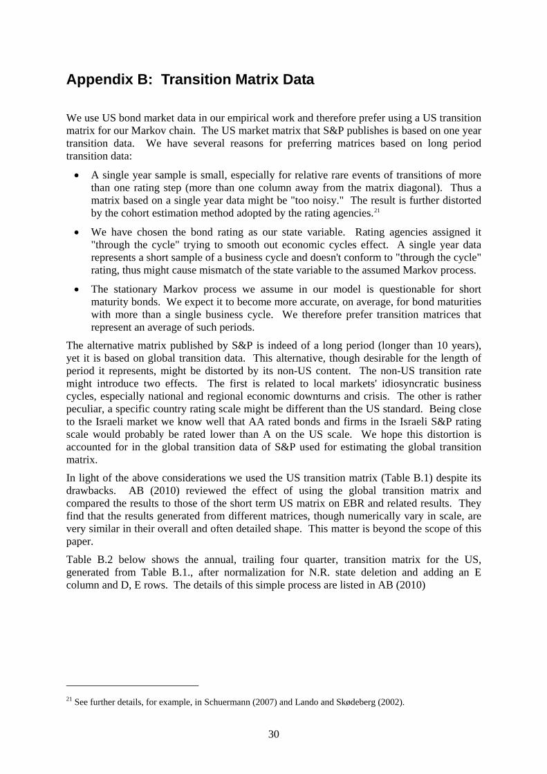
We use US bond market data in our empirical work and therefore prefer using a US transition matrix for our Markov chain. The US market matrix that S&P publishes is based on one year transition data. We have several reasons for preferring matrices based on long period transition data:

• A single year sample is small, especially for relative rare events of transitions of more than one rating step (more than one column away from the matrix diagonal). Thus a matrix based on a single year data might be "too noisy." The result is further distorted by the cohort estimation method adopted by the rating agencies.21

• We have chosen the bond rating as our state variable. Rating agencies assigned it "through the cycle" trying to smooth out economic cycles effect. A single year data represents a short sample of a business cycle and doesn't conform to "through the cycle" rating, thus might cause mismatch of the state variable to the assumed Markov process.

• The stationary Markov process we assume in our model is questionable for short maturity bonds. We expect it to become more accurate, on average, for bond maturities with more than a single business cycle. We therefore prefer transition matrices that represent an average of such periods.

The alternative matrix published by S&P is indeed of a long period (longer than 10 years), yet it is based on global transition data. This alternative, though desirable for the length of period it represents, might be distorted by its non-US content. The non-US transition rate might introduce two effects. The first is related to local markets' idiosyncratic business cycles, especially national and regional economic downturns and crisis. The other is rather peculiar, a specific country rating scale might be different than the US standard. Being close to the Israeli market we know well that AA rated bonds and firms in the Israeli S&P rating scale would probably be rated lower than A on the US scale. We hope this distortion is accounted for in the global transition data of S&P used for estimating the global transition matrix.

In light of the above considerations we used the US transition matrix (Table B.1) despite its drawbacks. AB (2010) reviewed the effect of using the global transition matrix and compared the results to those of the short term US matrix on EBR and related results. They find that the results generated from different matrices, though numerically vary in scale, are very similar in their overall and often detailed shape. This matter is beyond the scope of this paper.

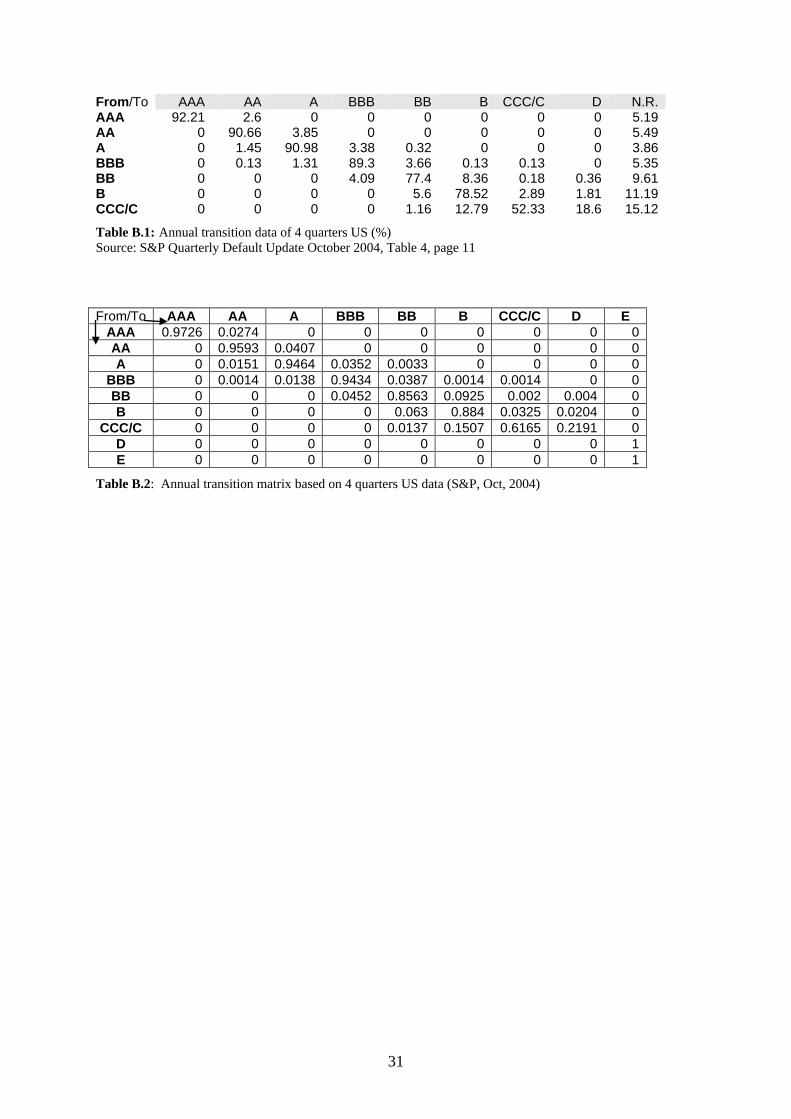
Table B.2 below shows the annual, trailing four quarter, transition matrix for the US, generated from Table B.1., after normalization for N.R. state deletion and adding an E column and D, E rows. The details of this simple process are listed in AB (2010)

21 See further details, for example, in Schuermann (2007) and Lando and Skødeberg (2002).

31

From/To AAA AA A BBB BB B CCC/C D N.R. AAA 92.21 2.6 0 0 0 0 0 0 5.19 AA 0 90.66 3.85 0 0 0 0 0 5.49 A 0 1.45 90.98 3.38 0.32 0 0 0 3.86 BBB 0 0.13 1.31 89.3 3.66 0.13 0.13 0 5.35 BB 0 0 0 4.09 77.4 8.36 0.18 0.36 9.61 B 0 0 0 0 5.6 78.52 2.89 1.81 11.19 CCC/C 0 0 0 0 1.16 12.79 52.33 18.6 15.12

Table B.1: Annual transition data of 4 quarters US (%) Source: S&P Quarterly Default Update October 2004, Table 4, page 11

From/To AAA AA A BBB BB B CCC/C D E

AAA 0.9726 0.0274 0 0 0 0 0 0 0 AA 0 0.9593 0.0407 0 0 0 0 0 0 A 0 0.0151 0.9464 0.0352 0.0033 0 0 0 0

BBB 0 0.0014 0.0138 0.9434 0.0387 0.0014 0.0014 0 0 BB 0 0 0 0.0452 0.8563 0.0925 0.002 0.004 0 B 0 0 0 0 0.063 0.884 0.0325 0.0204 0

CCC/C 0 0 0 0 0.0137 0.1507 0.6165 0.2191 0 D 0 0 0 0 0 0 0 0 1 E 0 0 0 0 0 0 0 0 1

Table B.2: Annual transition matrix based on 4 quarters US data (S&P, Oct, 2004)

32

Appendix C: Simplifying expressions including 1/T power Our aim in the following is to simplify the expressions that include the 1/T power using the general Binomial Theorem22:

(C.1) 0

(1 )v k

k

vx x

k

∞

=

+ =

∑ for v∈R ,

the series converges when |x|<1 which holds in our case where x = - probability ·(1-δ) in any practical case since probability and (1-δ) each ∈[0,1] , and probability <1.

The binomial coefficients (in the general case when v is not an integer) are defined by:23

(C.2) !

!( )!v vk k v k

= − and z! = Γ(z + 1)

(C.3) 2

0(1 ) 1 ... 1

2v k

k

v vx x v x x v x

k

∞

=

+ = = + ⋅ + + ≈ + ⋅

∑

Rational for the above approximation:

v = 1/T thus the binomial coefficient diminishes from k = 2 term (see Figure C.1 below) and:

|x| = probability of default times (1-δ) < 0.2·(1-0.2) ≈ 0.15 for a speculative-grade bond with two years to maturity and a low recovery rate of 0.2.24 Typical recovery rates are 0.4 and πD < 0.02 (for a B bond), hence typically |x| < 0.008. Therefore typically k=2 series element is smaller than 10-5 and is below 0.003 for the above speculative-grade bond with two years to maturity and a very low recovery rate. The k=3 series element is much smaller.

We therefore use the following approximation:

(C.4) ( ) ( )1/ 11 1 1 1

T

D DTπ δ π δ − − ≈ − −

An example for a “large error: (1- 0.2·0.8)0.5 = 0.9165 whereas the approximation 1 – 0.5· 0.2·0.8 = 0.9200 differs only by 0.0035 from the accurate result. Typically the error is much smaller (e.g. <1.5·10-5 for 10 years to maturity with recovery of 0.4).

22 See for example: http://mathworld.wolfram.com/BinomialTheorem.html where additional information and references are provided. 23 See for example: http://mathworld.wolfram.com/BinomialCoefficient.html 24 See Figure C.2 for default probabilities of various bonds.

33

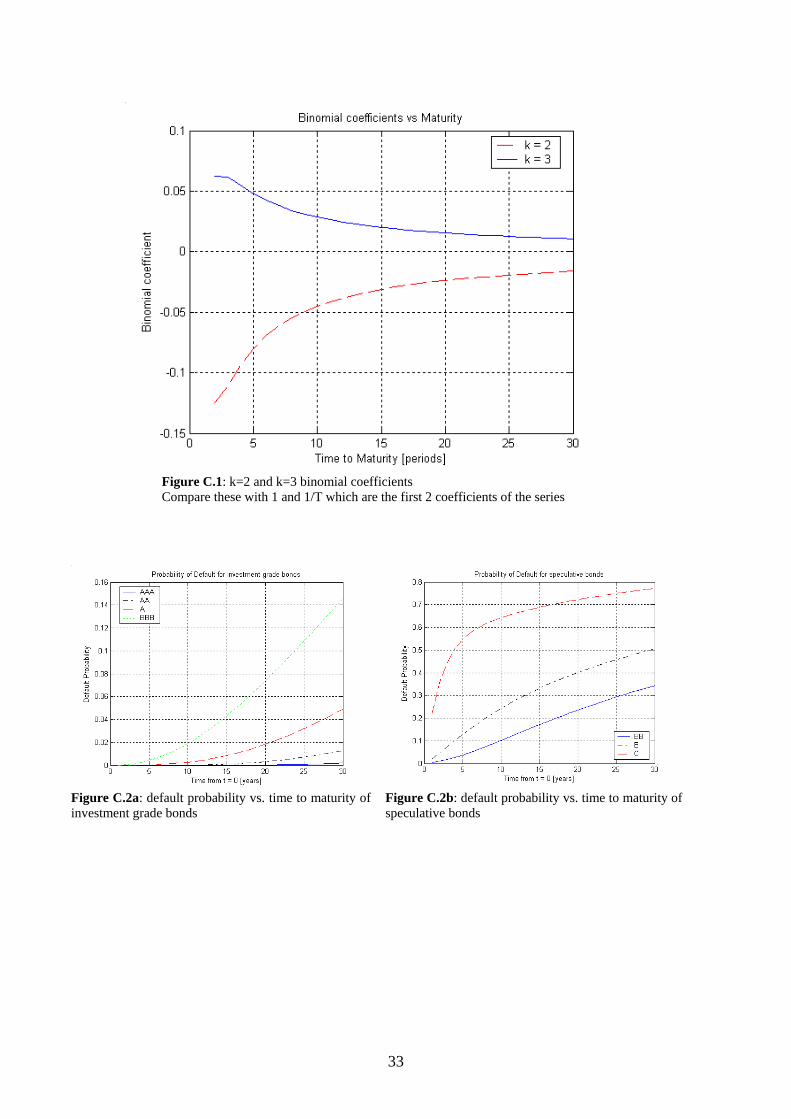
Figure C.1: k=2 and k=3 binomial coefficients Compare these with 1 and 1/T which are the first 2 coefficients of the series

Figure C.2a: default probability vs. time to maturity of investment grade bonds

Figure C.2b: default probability vs. time to maturity of speculative bonds

34

Appendix D: Input Data Characteristics

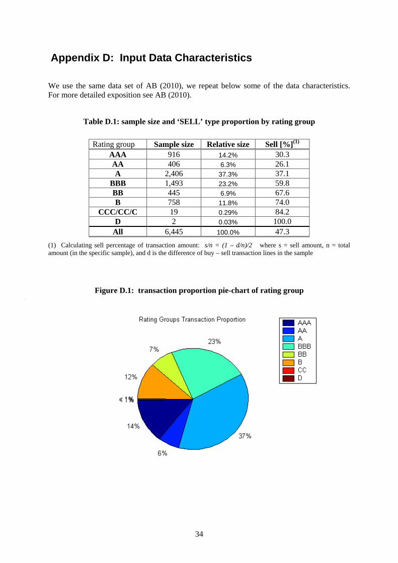
We use the same data set of AB (2010), we repeat below some of the data characteristics. For more detailed exposition see AB (2010).

Table D.1: sample size and ‘SELL’ type proportion by rating group

Rating group Sample size Relative size Sell [%](1) AAA 916 14.2% 30.3 AA 406 6.3% 26.1 A 2,406 37.3% 37.1

BBB 1,493 23.2% 59.8 BB 445 6.9% 67.6 B 758 11.8% 74.0

CCC/CC/C 19 0.29% 84.2 D 2 0.03% 100.0

All 6,445 100.0% 47.3 (1) Calculating sell percentage of transaction amount: s/n = (1 – d/n)/2 where s = sell amount, n = total amount (in the specific sample), and d is the difference of buy – sell transaction lines in the sample

Figure D.1: transaction proportion pie-chart of rating group

35

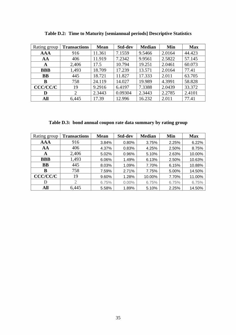
Table D.2: Time to Maturity [semiannual periods] Descriptive Statistics

Rating group Transactions Mean Std-dev Median Min Max AAA 916 11.361 7.1559 9.5466 2.0164 44.423 AA 406 11.919 7.2342 9.9561 2.5822 57.145 A 2,406 17.5 10.794 19.251 2.0461 60.073

BBB 1,493 18.709 17.239 13.571 2.0164 77.41 BB 445 18.721 11.827 17.333 2.011 63.705 B 758 24.119 14.027 19.989 4.3991 58.828

CCC/CC/C 19 9.2916 6.4197 7.3388 2.0439 33.372 D 2 2.3443 0.09304 2.3443 2.2785 2.4101

All 6,445 17.39 12.996 16.232 2.011 77.41

Table D.3: bond annual coupon rate data summary by rating group

Rating group Transactions Mean Std-dev Median Min Max AAA 916 3.84% 0.80% 3.75% 2.25% 6.22% AA 406 4.37% 0.83% 4.25% 2.50% 8.75% A 2,406 5.02% 0.96% 5.10% 2.63% 10.00%

BBB 1,493 6.06% 1.49% 6.13% 2.50% 10.63% BB 445 8.03% 1.09% 7.70% 6.15% 10.88% B 758 7.59% 2.71% 7.75% 5.00% 14.50%

CCC/CC/C 19 9.60% 1.28% 10.00% 7.70% 11.00% D 2 6.75% 0.00% 6.75% 6.75% 6.75%

All 6,445 5.58% 1.89% 5.10% 2.25% 14.50%

36

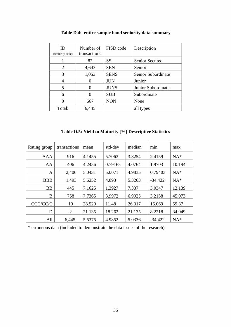
Table D.4: entire sample bond seniority data summary

ID (seniority code)

Number of transactions

FISD code Description

1 82 SS Senior Secured 2 4,643 SEN Senior 3 1,053 SENS Senior Subordinate 4 0 JUN Junior 5 0 JUNS Junior Subordinate 6 0 SUB Subordinate 0 667 NON None

Total: 6,445 all types

Table D.5: Yield to Maturity [%] Descriptive Statistics

Rating group transactions mean std-dev median min max

AAA 916 4.1455 5.7063 3.8254 2.4159 NA*

AA 406 4.2456 0.79165 4.0764 1.9703 10.194

A 2,406 5.0431 5.0071 4.9835 0.79403 NA*

BBB 1,493 5.6252 4.893 5.3263 -34.422 NA*

BB 445 7.1625 1.3927 7.337 3.0347 12.139

B 758 7.7365 3.9972 6.9025 3.2158 45.073

CCC/CC/C 19 28.529 11.48 26.317 16.069 59.37

D 2 21.135 18.262 21.135 8.2218 34.049

All 6,445 5.5375 4.9852 5.0336 -34.422 NA*

* erroneous data (included to demonstrate the data issues of the research)

37

Appendix E: List of Abbreviations

BS bond spread

CDS credit default swap

CEP certainty equivalence premium

CRP credit risk premium

CUSIP Committee on Uniform Securities Identification Procedures

EBR expected bond return

FISD Fixed Income Securities Database

ISIN International Securities Identification Number

JLT Jarrow, Lando, and Turnbull

NASD The National Association of Securities Dealers

NR not rated

NS Nelson-Siegel

RN risk-neutral

S&P Standard and Poor's

SIC Standard Industrial Classification

TM transition matrix

TRACE Trade Reporting and Compliance Engine

TS term structure

TSIR term structure of interest rates

ytm yield to maturity