The Cross-Section of Expected Corporate

Bond Returns∗

Jennie Bai† Turan G. Bali‡ Quan Wen§

Abstract

This study constructs risk factors that are important for the pricing of corporate bond.We find that expected corporate bond returns are related cross-sectionally to downsiderisk, credit risk, liquidity risk, and bond market risk. Based on these risk proxies, weconstruct three bond-implied risk factors: DRF, CRF, and LRF. Our new factors rely onthe unique features of corporate bonds that distinguish from stocks, hence have superiorperformance in explaining the cross-section of expected bond returns, than all establishedstock and bond market factor models.

This Version: May 2016

Keywords :

JEL Classification: G10, G11, C13.

∗We thank...for their extremely helpful comments and suggestions. We also thank Kenneth French, LubosPastor, and Robert Stambaugh for making a large amount of historical data publicly available in their onlinedata library. All errors remain our responsibility.†Assistant Professor of Finance, McDonough School of Business, Georgetown University, Washington, D.C.

20057. Phone: (202) 687-5695, Fax: (202) 687-4031, Email: Jennie.Bai@georgetown.edu‡Robert S. Parker Chair Professor of Finance, McDonough School of Business, Georgetown University,

Washington, D.C. 20057. Phone: (202) 687-5388, Fax: (202) 687-4031, Email: Turan.Bali@georgetown.edu§Assistant Professor of Finance, McDonough School of Business, Georgetown University, Washington, D.C.

20057. Phone: (202) 687-6530, Fax: (202) 687-4031, Email: Quan.Wen@georgetown.edu

1 Introduction

In the past three decades, researchers have identified many risk factors in the cross section

of stock returns. However, far fewer studies are devoted to the cross section of corporate

bond returns. Compared to the size of the U.S. stock market, $29 trillions, the corporate

bond market is relatively small with an outstanding of $12 trillions.1 However, the issuance

of corporate bond is in much larger scale than the issuance of stocks for the United States

corporations, on average $1,294 billions for corporate bonds compared to $265 billions for stocks

since 2010. Both corporate bonds and stocks are important financing channels for corporations,

and both are important assets under management for practitioners. It’s important to enhance

our understanding of the risk-return relationship in the corporate bond market.

Conventional corporate bond studies rely on the long-established stock and bond fac-

tors to predict the corporate bond expected returns, including the five factors of Fama and

French (1993), Carhart (1997) and Pastor and Stambaugh (2003): the excess stock market re-

turn (MKT), the size factor (SMB), the book-to-market factor (HML), the momentum factor

(MOM), and the liquidity factor (LIQ), and the excess bond market return (Elton, Gruber, and

Blake (1995)), the default spread (DEF) and the term spread (TERM). In this paper, we show

that it is crucial to respect the unique features of corporate bonds and construct bond-implied

risk factors to explain the cross-section of corporate bond returns.

Although corporate bonds and stocks both reflect firm fundamentals, they differ in several

key features. First and foremost, firms issue corporate bonds suffer from the potential default

risk given the legal requirement on the payments of coupons and principals, whereas firms

issue stocks only have negligible exposure to bankruptcy. This main feature makes credit risk

in particular important in determining corporate bond returns.

Second, bondholders compared with stockholders are more sensitive to downside risk. Bond-

holders gain the cash flow of fixed coupon and principal payment, thus hardly benefit from the

euphoric news in the firm fundamentals. Since the upside payoffs are capped, the bond pay-

offs become concave in the investor beliefs about the underlying fundamental, whereas equity

payoffs are linear in the investor beliefs regarding the underlying fundamental.

1Source: Table L.213 and L.223 in the Federal Reserve Board’s Z1 Flow of Funds, Balance Sheets, andIntegrated Macroeconomic Accounts, as of the fourth quarter of 2015.

1

Third, the corporate bond market, due to its over-the-counter trading mechanism and

other market features, bears higher liquidity risk. The bond market participants have been

dominated by institutional investors such as insurance companies, pension funds, and mutual

funds.2 Many bondholders are long-term investors who often take the buy-and-hold strategy.

Therefore the liquidity in the corporate bond market is lower compared with the stock market

in which active trading is partially contributed by the existence of individual (noisy) traders.

Given these special features in the corporate bond market, we endeavor to identify bond-

implied risk factors. In particular, we examine the pricing power of downside risk, credit

risk, and liquidity risk on the cross-section of expected corporate bond returns. The bond

returns are calculated at the monthly frequency using the intraday trasaction records from

the enhanced TRACE data from July 2002 to December 2014, a total of 507,714 bond-month

observations. Our proxy for downside risk is the 5% Value-at-Risk (VaR) which is based on

the lower tail of the empirical return distribuition, that is, the second lowest monthly return

observation over the past 36 months. Our proxy for credit risk is bond-level credit rating.

Our proxy for liquidity risk is bond-level illiquidity measure following Bao, Pan, and Wang

(2011). In the online appendix, we also consider alternative proxies for downside risk, credit

risk, and liquidity risk, and results remain robust. In addition to these three bond risk proxies,

we further consider the market risk factor based on the corporate bond market index instead

of conventional stock market index, and construct the bond market β.

First, we test the significance of a cross-sectional relation between downside risk and future

returns on corporate bonds using portfolio-level analysis. We find that bonds in the highest

VaR quintile generate 9.43% per annum higher return than bonds in the lowest VaR quintile

do. After controlling seven long-established stock and bond factors, the risk-adjusted return

premium from the lowest to the highest VaR quintile is still about 8.52% with a t-statistic

of 3.85, suggesting that loss-averse bond investors prefer high expected return and low VaR.

We investigate the source of the significant return spread between high- and low-VaR bonds,

and find that the significantly positive return spread is due to outperformance by high-VaR

2 According to the balance sheet of corporate bonds in 2014:Q4, reported by the Federal Reserve release,the main holders of corporate bond are insurance industries which hold $2678 billion, pension and retirementfunds which hold $983 billion, mutual funds, close-end funds and exchange-traded funds which together hold$2502 billion. Source: the Financial Accounts of the United States, Release Z1, Table L.213, Line 19 – 47.

2

bonds, but not to underperformance by low-VaR bonds. We also test if the positive relation

between downside risk and future returns holds controlling for bond characteristics, and find

that downside risk remains a significant predictor after controlling for credit rating, bond

maturity and size.

Second, we examine the cross-sectional relation between credit risk, liquidity risk and future

bond returns. We find that corporate bonds in the highest credit risk quintile generate 7.80%

to 5.09% more raw and risk-adjusted returns per annum compared to bonds in the lowest

credit risk quintile. In addition, the significantly positive credit risk premium is driven by

bonds with high credit risk, but not by bonds with low credit risk. Examining the portfolio

bond characteristics, we also find that high credit risk bonds tend to have higher downside

risk, higher illiquidity, shorter maturity, and smaller size, but not significantly different market

betas. The results for the cross-sectional relation between liquidity risk and bond returns

are similar. Corporate bonds in the highest illiquidity quintile generate 6.42% to 6.35% more

raw and risk-adjusted returns per annum compared to bonds in the lowest illiquidity quintile.

Bonds in the high illiquidity quintile also tend to have higher downside risk, higher bond market

beta, longer maturity, and smaller size, though not significantly different credit risk.

Third, we particularly investigate whether the CAPM holds in the corporate bond market.

Specifically, we test if the CAPM with the bond market factor explains the cross-sectional

corporate bond returns. We find that the market factor based on the stock market index such

as S&P 500 or CRSP cannot explain the cross-section of expected bond returns; however, the

market factor based on the Merrill Lynch Aggregate Bond market index has significant and

positive predicting power. Bonds in the high bond market beta quintile generates 7.07% to

6.68% higher raw and risk-adjusted returns per annume compared to bonds in the low market

beta quintile. Moreover, the significantly positive bond market risk premium is driven by bonds

with high beta, whereas bonds with low beta have insignificant average return.

After combining all bond risk proxies and controlling bond characteristics in the Fama-

MacBeth regression, downside risk and liquidity risk stand out with significance, whereas the

pricing power of credit risk and bond market risk weakens or disappears.

Finally, we propose three novel risk factors based on the aforementioned bond risk proxies:

downside risk factor (DRF ), credit risk factor (CRF ), and liquidity risk factor (LRF ), in the

3

similar spirit of Fama and French (1993, 1996) constructing stock market risk factors. We show

that when regressing each of new risk factors on long-established stock and market factors, all

intercepts (alphas) are statistically and economically significant and the adjusted-R2 values are

relatively low, suggesting that the existing common risk factors are not sufficient to capture

the information contained in these new bond risk factors. We further form test portfolios using

corporate bond returns and examine the explanatory power of our bond risk factors and that of

alternative factor models. Either for the 10 decile portfolios sorted by bond size, or for the 10

decile portfolios sorted by bond maturity, or for the 25 portfolios sorted by size and maturity,

our newly proposed bond risk factor model has the greatest explanatory power compared with

three benchmark factors models based on the literature. For example, the difference of average

R2 values between our model and the Fama-French five-factor model is 0.80 vs 0.41 for size-

sorted 10 portfolios, 0.81 vs 0.47 for maturity-sorted 10 portfolios, and 0.78 vs 0.41 for size and

maturity sorted 25 portfolios. These results suggest that the newly proposed bond risk factors

capture common variations of the cross-section corporate bond returns, which cannot be fully

characterized by the existing stock and/or bond market risk factors.

In the following sections, we describes the data, test the pricing power of bond character-

istics, construct three new risk factors and show their superior performance in explaining the

cross-section of expected bond returns.

2 Data

2.1 Corporate Bond Data

For corporate bond data, we rely on the transaction records reported in the original and en-

hanced version of the Trade Reporting and Compliance Engine (TRACE) for the sample period

of July 2002 to December 2014. Ideally, we hope to understand the risk-return relationship

using a longer sample period; however, one crucial factor to study corporate bond returns, the

illiquidity, requires the daily bond transaction prices which are not provided in data sets such

4

as Lehman Brothers fixed income database, Datastream, or Bloomberg.3 Therefore, we focus

on the TRACE data which offers the best quality of corporate bond transactions with intraday

observations on price, trading volume, buy and sell indicator. We then merge corporate bond

pricing data merged with Mergent fixed income securities database to collect bond character-

istics such as offering amount, offering date, maturity date, coupon rate, coupon type, interest

payment frequency, bond type, bond rating, bond option features, and issuer information.

In the online appendix A.2, we also expand our dataset to include alternative bond data

sets, mainly containing quoted prices, for a longer sample period starting from January 1973.

With this longer sample, we replicate our analysis except those requring an illiquidity measure.

For TRACE data, we adopt the filtering criteria proposed in Bai, Bali, and Wen (2016).

Concisely, we remove bonds i) that are not listed or traded in the U.S. public market; ii)

that are structured notes, mortgage backed or asset backed, agency-backed or equity-linked;

iii) that are convertible; iv) that trade under five dollars or above one thousand dollars; v)

that have floating coupon rates; and bonds vi) that have less than one year to maturity. For

intraday data, we also eliminate bond transactions vii) that are labeled as when-issued, locked-

in, or have special sales conditions; viii) that are canceled, x) that have more than two-day

settlement, and xi) that have trading volume smaller than $100,000. We adjust records that

are subsequently corrected or reversed.

2.2 Corporate Bond Return

The monthly corporate bond return at time t is computed as

Ri,t =Pi,t + AIi,t + Ci,tPi,t−1 + AIi,t−1

− 1 (1)

where Pi,t is the transaction price, AIi,t is accrued interest, and Ci,t is the coupon payment, if

any, of bond i in month t.

With the TRACE intraday data, we first calculate the daily clean price as the trading

3The National Association of Insurance Commissioners database (NAIC) also includes daily prices but giventhe fact that it covers only part of the market and it is more illiquid, transactions only by the buy-and-holdinsurance companies, combining this data with TRACE does not make a compatible sample. For consistency,we focus on the TRACE data.

5

volume-weighted average of intraday prices in order to minimize the effect of bid-ask spreads

in prices, following Bessembinder, Kahle, Maxwell, and Xu (2009). We then convert the bond

prices from daily to monthly following Bai, Bali, and Wen (2016) which has a detailed discussion

on the conversion methods in the literature. In detail, the method identifies three scenarios

for a return to be realized at the end of month t: 1) from the end of month t− 1 to the end of

month t, 2) from the beginning of month t to the end of month t, and 3) from the beginning of

month t to the beginning of month t+ 1. We calculate monthly returns for all three scenarios,

where the end (beginning) of month refers to the last (first) five trading days within each

month. If there are multiple trading records in the five-day window, the one closest to the last

trading day of the month will be selected. If a monthly return can be realized in more than

one scenario, the realized return in scenario one (from month-end t − 1 to month-end t) will

be selected.

Our final sample includes 13,425 bonds issued by 2,178 unique firms, a total of 507,714

bond-month return observations during the sample period of July 2002 to December 2014.

On average, there are about 3,530 bonds per month over the whole sample. Panel A of

Table 1 reports the time-series average of the cross-sectional bond returns’ distribution and

bond characteristics. The average monthly bond return is 0.39%, which corresponds to 4.68%

per annum. The sample contains bonds with an average rating of 8.06 (i.e., BBB+), an average

issue size of 396 millions of dollars, and an average of time-to-maturity of 12.74 years. Among

the full sample of bonds, about 90% are investment-grade and the remaining 10% are high-yield

bonds.

3 Cross-sectional Predictors

In this section, we aim to identify several bond risk proxies and evaluate their power to explain

the cross-section of bond returns. Corporate bonds provide an attractive setting to study these

issues because there are few studies examine the cross-section of corporate bond returns in the

empirical asset pricing literature and because the risk factors are easier to identify (Gebhardt,

Hvidkjaer, and Swaminathan (2005)). Among these, Fama and French (1993) first show that

default and term premia are important risk factors for corporate bond pricing, in addition to

6

the commonly used Fama-French three factors (e.g., the stock market excess returns, the size

factor, and the book-to-market factor). Gebhardt, Hvidkjaer, and Swaminathan (2005) test the

pricing power of default beta and term beta and find that they are significantly related to the

cross-section of bond returns, even after controlling for a large number of bond characteristics.

Lin, Wang, and Wu (2011) construct the market liquidity risk factor and show that it is priced

in the cross-section of corporate bond returns.

The strand of literature that study the cross-section of corporate bond returns tend to use

the commonly used stock market factors. This is a natural starting point since rational pricing

suggests that risk premia in the equity market should be consistent with the corporate bond

market, to the extent that two markets are integrated. First, because both bond and stock are

contingent claims on the value of the same underlying assets, stock market factors such as size

and book-to-market equity should share common variations in stock and bond returns (e.g.,

Merton (1974)). Second, expected default loss of corporate bonds changes with equity price.

Default risk decreases as the equity value appreciates, and this induces a systematic factor that

affects corporate bond returns.

However, corporate bond market has its unique features. First and foremost, firms that

issue corporate bonds suffer from the potential default risk given the legal requirement on

the payments of coupons and principals, whereas firms that issue stocks have only negligible

exposure to bankruptcy. This main disparity makes credit risk particularly important in deter-

mining corporate bond returns. Second, bondholders are more sensitive to downside risk than

stockholders. Bondholders gain the cash flow of fixed coupon and principal payments and,

thus hardly benefit from the euphoric news in firm fundamentals. Since the upside payoffs are

capped, the bond payoff relation with investor beliefs about the underlying fundamental be-

comes concave, whereas the equity payoff relation with investor beliefs regarding the underlying

fundamental is linear (e.g., Hong and Sraer (2013)).

Third, the corporate bond market is much less liquid than the equity market with most

corporate bonds trading infrequently. Thus, both the level of liquidity and liquidity risk are

serious concern for investors in the corporate bond market. Fourth, the corporate bond mar-

ket participants have been dominated by institutional investors such as insurance companies,

pension funds, and mutual funds, whose attitudes toward risk may differ significantly from in-

7

dividual investors.4 Lastly, there is abundant evidence that shows the discrepancies in return

premia between equity and corporate bond markets (e.g., Choi and Kim (2015); Chordia et al.

(2015)), thus suggesting potential market segmentation.

3.1 Downside Risk

We measure downside risk of corporate bonds using Value-at-Risk (VaR). VaR determines how

much the value of an asset could decline over a given period of time with a given probability

as a result of changes in market rates or prices. For example, if the given period of time is one

day and the given probability is 1%, the VaR measure would be an estimate of the decline in

the asset’s value that could occur with 1% probability over the next trading day. Our proxy for

downside risk, 5% VaR, is based on the lower tail of the empirical return distribution, that is,

the second lowest monthly return observation over the past 36 months. We then multiply the

original measure by −1 for the convenience of interpretation.5 As shown in Table 1, the average

downside risk is 6.43% in the whole sample with a standard deviaion of 3.87%. Section 4 will

further discuss the importance of downside risk to bondholders and test their pricing power on

the cross-sectional expected corporate bond returns.

3.2 Credit Risk

To measure the credit risk of corporate bonds, we rely on corporate bond credit ratings. Credit

ratings capture information on bond default probability, and hence is the benchmark choice

to measure the credit risk of corporate bonds. We collect bond-level rating information from

Mergent FISD historical ratings. All ratings are assigned a number to facilitate the analysis,

for example, 1 refers to a AAA rating, 2 refers to AA+, 21 refers to CCC, and so forth.

Investment-grade bonds have ratings from 1 (AAA) to 10 (BBB-). Non-investment-grade

bonds have ratings above 10. A larger number suggests higher credit risk, or lower credit

4Institutional investors in particular make extensive use of corporate bonds in constructing their portfolios.According to flow of fund data during 1986-2012, about 82% of corporate bonds were held by institutionalinvestors including insurance companies, mutual funds and pension funds. The participation rate of individualinvestors in the corporate bond market is very low.

5Note that the original maximum likely loss values are negative since they are obtained from the left tailof the return distribution. After multiplying the original VaR measure by −1, a positive regression coefficientcan be explained as the higher downside risk is related to the higher cross-sectional bond returns.

8

quality. In section 5.1, we test the pricing power of credit risk, as measured by bond credit

rating, in the cross-section of expected corporate bond returns.

3.3 Liquidity Risk

The literature has documented the importance of illiquidity and liquidity risk in the corporate

bond market. For example, the empirical results in Chen, Lesmond, and Wei (2007), and

Dick-Nielsen, Feldhutter, and Lando (2012) have established the relation between corporate

bond yield spreads and bond illiquidity. Using transactions data from 2003 to 2009, Bao, Pan,

and Wang (2011) show that the bond-level illiquidity explains a substantial cross-sectional

variations in bond yield spreads. Lin, Wang, and Wu (2011) construct a liquidity risk factor

for the corporate bond market and show that the market liquidity beta is priced in the cross-

section of corporate bond returns. Given the importance of the transaction-based data such

as TRACE for measuring bond illiquidity, we follow Bao, Pan, and Wang (2011) to construct

bond-level illiquidity. The illiquidity measure, ILLIQ, is aimed at extracting the transitory

component from bond price. Specifically, let ∆pt = pt− pt−1 be the log price change from t− 1

to t. Then, ILLIQ is defined as

ILLIQ = −Covt(∆pitd,∆pitd+1), (2)

where ∆pitd is the price change for bond i on day d of month t. In section 5.2, we test the

pricing power of bond illiquidity in the cross-section of expected corporate bond returns.

3.4 Bond Market β

In the capital asset pricing model test, the market model almost unanimously adopts the excess

stock market return as the factor. This is motivated by the observation that if markets are

integrated, a single model that explains equity returns should also explain bond returns (Fama

and French (1993)). However, as pointed out by Elton, Gruber, and Blake (1995), the best

candidate in a single factor model that best explains individual bond returns would be an

index of aggregate bond returns. Following Elton, Gruber, and Blake (1995), we identify our

9

first corporate bond risk factor as the excess bond market returns. The bond market factor is

designed to mimic the common variation in corporate bond returns related to the aggregate

bond market returns. We use the Merrill Lynch U.S. Aggregate Bond Index as a proxy for the

corporate bond market factor.6 Our first bond risk factor, the bond market return (MKTBond),

is computed as the percentage change in the monthly Merrill Lynch Bond Index values. We

also estimate bond market beta, βBond, for each bond from the time-series regressions of bond

excess returns on the excess bond market return, with a 36-month rolling window. As shown

in Table 1, the bond beta has a wide range from -0.39 in the 1st percentile to 3.20 in the 99th

percentile, with an average value of 1.10 over the whole sample. In section 5.3, we investigate

whether CAPM holds in the corporate bond market. Specifically, we test if the CAPM with

the bond market factor explains the cross-sectional differences in expected returns on corporate

bonds.

Panel B of Table 1 presents the correlations between different bond risk proxies and bond

characteristics. It is worth noting that bond market beta, βBond, is positively correlated with all

other variables, with correlation coefficients ranging from 0.08 to 0.49. Among them, downside

risk has the highest correlation with βBond with a value of 0.49, implying that bonds with

higher downside risk have high market risk as well. Bond maturity has the second highest

correlation with βBond with a value of 0.32. Bond illiquidity is also positively correlated with

downside risk, with a value of 0.24. In sum, bonds with higher downside risk tend to be those

also having higher credit risk, higher illiquidity, and higher market risk. In the next session,

we provide new empirical evidence that downside risk, as measured by Value-at-Risk (VaR),

is significantly priced in the cross-section of expected corporate bond returns.

4 Pricing Power of Downside Risk

4.1 Motivation

Downside risk captures the exposure to losses. That is, it is the risk of the actual return being

below the expected return, or the uncertainty about the magnitude of that difference. We con-

6We also consider alternative proxies such as the Barclays Aggregate Bond Index, the equal-weighted andvalue-weighted corporate bond market index using the sample in our paper, and the results remain similar.

10

sider Value-at-Risk (VaR) as the proxy to determines how much the value of a corporate bond

could decline over a given period of time with a given probability. Bai, Bali, and Wen (2016)

investigate the distributional features of corporate bonds, volatility, skewness, and kurtosis,

and find that the empirical distribution of bond returns is skewed, peaked around the mode,

and has fat-tails, implying that extreme returns occur much more frequently than predicted

by the normal distribution. Downside risk measures, accounting for higher-order moments of

the return distribution, provide more accurate estimates of actual losses and produce good

predictions of market risk during extraordinary periods such as bond market collapses.

From investors’ perspective, investors in the corporate bond market are more cautious

than those in the stock market. Bondholders gain the cash fow of fixed coupon and principal

payments and, thus hardly benefit from the euphoric news in firm fundamentals. Since the

upside payoffs are capped, the bond payoff relation with investor beliefs about the underlying

fundamental becomes concave, whereas the equity payoff relation with investor beliefs regarding

the underlying fundamental is linear (Hong and Sraer (2013)). Table A.1 of the appendix

estimates the risk aversion parameter for the corporate bond and stock markets. Proxies for

the corporate bond market are the Merrill Lynch U.S. aggregate bond index, the equal-weighted

and value-weighted indexes of all corporate bonds in our sample. Proxies for the stock market

are the Standard & Poor’s ( S&P) 500 index and the value-weighted CRSP index which includes

all stocks trading on the NYSE, AMEX, and NASDAQ.

We use both conditional and unconditional approaches to estimate the risk aversion param-

eter (see Section A.1). Table A.1 shows that the conditional approach based on the GARCH-

in-mean model yields the risk aversion parameter for a typical corporate bond market investor

in the range of 12.1 to 14.7. The unconditional approach yields similar estimates of risk aver-

sion for an average bond market investor, in the range of 12.3 to 16.6. The risk aversion for

a typical stock market investor however is much lower: 5.5 for the S&P500 index and 7.5 for

the value-weighted CRSP index if using the conditional approach; and even lower if using the

unconditional approach: 3.5 for the S&P500 index and 3.7 for the value-weighted CRSP index.

Overall, these findings provide evidence that corporate bond investors are more risk averse

and more sensitive to downside risk. To evaluate the risk-return relationship in the corporate

bond market, downside risk is quintessential. We appraise the pricing power of downside risk

11

in the next subsection.

4.2 Univariate Portfolio Analysis

We first examine the significance of a cross-sectional relation between VaR and future corporate

bond returns using portfolio analysis. For each month from July 2004 to December 2014, we

form quintile portfolios by sorting corporate bonds based on their downside risk (VaR), where

quintile 1 contains bonds with the lowest downside risk, and quintile 5 contains bonds with

the highest downside risk.7 Table 2 shows the average VaR values of bonds in each quintile,

the next month average excess return, and the 7-factor alpha for each quintile. The last

five columns report the average bond characteristics for each quintile including bond beta,

illiquidity, creidt rating, time-to-maturity, and bond size. The last row displays the differences

of average returns or the alphas between quintile 5 and quintile 1. Average excess returns and

alphas are defined in terms of monthly percentage. Newey-West (1987) adjusted t-statistics

are reported in parentheses.

Moving from quintile 1 to quintile 5, the average excess return on the downside risk port-

folios increases monotonically from -0.137% to 0.649% per month. This indicates a monthly

average return difference of 0.786% between quintiles 5 and 1 (i.e., High-VaR quintile vs. Low-

VaR quintile) with a Newey-West t-statistic of 3.19, showing that this positive return difference

is statistically and economically significant. This result also indicates that corporate bonds in

the highest VaR quintile generate 9.43% per annum higher return than bonds in the lowest

VaR quintile do.

In addition to the average excess returns, Table 2 also presents the alphas from the regression

of the quintile portfolio returns on well-known stock and bond market factors — the excess

stock market return (MKT), a size factor (SMB), a book-to-market factor (HML), a momentum

factor (MOM), and a liquidity factor (LIQ), following Fama and French (1993), Carhart (1997),

and Pastor and Stambaugh (2003), and the default spread factor (DEF) and the term spread

factor (TERM), following Elton et al. (2001), and Bessembinder et al. (2009). Similar to

7Downside risk is measured by the 5% VaR using a 36-month rolling window. A bond is included in oursample if it has at least 24 monthly return observations in the 36-month rolling window before the test month.Our data start in July 2002 and we report portfolio results starting from July 2004.

12

the average excess returns, the 7-factor alpha on the downside risk portfolios also increases

monotonically from -0.207% to 0.503% per month, moving from the low-VaR to the high-VaR

quintile, indicating a positive and significant alpha difference of 0.710% per month (t-statistic

= 3.85). This result suggests that loss-averse bond investors prefer high expected return and

low VaR.

Next, we investigate the source of significant alpha spread between high-VaR and low-VaR

bonds. As reported in Table 2, the alphas in quintile 1 (low-VaR bonds) are statistically

insignificant, whereas the alphas in quintile 5 (high-VaR bonds) are economically and statisti-

cally positive significant. Therefore, we conclude that the significant and positive alpha spread

between high-VaR and low-VaR bonds is due to the outperformance of high-VaR bonds, but

not due to the underperformance of low-VaR bonds.

Lastly, we examine the average characteristics of VaR-sorted portfolios. As shown in the last

five columns of Table 2, bonds with high downside risk have higher market beta, higher level of

trading illiquiduity, higher credit risk, longer time-to-maturity, and smaller size. This creates

a potential concern about the interaction between downside risk and bond characteristics. We

provide different ways of handling this concern. Specifically, we test whether the positive

relation between VaR and the cross-section of bond returns holds once we control for credit

rating, maturity, and size based on bivariate portfolio sorts and Fama-MacBeth regressions in

the following subsections.

4.3 Controlling for Bond Characteristics

Table A.2 of the online appendix presents the results from the bivariate sorts of VaR and bond

characteristics. In Panel A of Table A.2, quintile portfolios are formed by first sorting corporate

bonds into five quintiles based on their credit ratings; then, within each rating portfolio, bonds

are sorted further into five sub-quintiles based on their VaR. This methodology, under each

rating-sorted quintile, produces sub-quintile portfolios of bonds with dispersion in downside

risk but have nearly identical ratings. VaR,1 represents the lowest VaR-ranked bond quintiles

within each of the five rating-ranked quintiles. Similarly, VaR,5 represents the highest VaR-

ranked quintiles within each of the five rating-ranked quintiles.

13

Panel A of Table A.2 shows that the alphas under 5- and 7-factor model increase mono-

tonically from the VaR,1 to the VaR,5 quintile. More importantly, after controlling for credit

rating, the 7-factor alpha differences between high- and low-VaR bonds remain positive, about

0.634% per month, and highly significant with t-statistics of 4.23. We further investigate the

interaction between VaR and credit ratings by sorting investment-grade and non-investment-

grade bonds separately into bivariate quintile portfolios. As expected, the positive relation

between VaR and expected returns is stronger for non-investment-grade bonds with the alpha

spread of 0.730% per month (t-stat= 3.88), but the significantly positive relationship remains

for investment-grade bonds even after we control for credit ratings, with the alpha spread of

0.463% per month (t-stat= 2.97).

Panel B of Table A.2 presents the results from the bivariate sorts of downside risk and

maturity. Quintile portfolios are formed by first sorting corporate bonds into five quintiles

based on their maturity; then, within each maturity portfolio, bonds are sorted further into

five sub-quintiles based on their VaR. Panel B shows that after controlling for bond maturity,

the alpha differences between high- and low-VaR bonds remain positive, 0.661% per month,

and highly significant with t-statistics of 4.07. We further examine the interaction between

VaR and maturity by sorting short-maturity bonds (1 year ≤ maturity ≤ 5 years), medium-

maturity bonds (5 years < maturity ≤ 10 years), and long-maturity bonds (maturity > 10

years) separately into bivariate quintile portfolios based on their VaR and maturity. After

controlling for maturity, the alpha spread between the VaR,1 and VaR,5 quintiles is 0.576% per

month and marginally significant for short-maturity bonds, 0.615% per month and significant

for medium-maturity bonds, and about 0.626% per month and significant for long-maturity

bonds. Although the economic significance of these alpha spreads is similar across the three

maturity groups, the statistical significance of the alpha differences is greater for medium- and

long-maturity bonds. This result makes sense because longer-term bonds usually offer higher

interest rates, but may entail additional risks.8

Panel C of Table A.2 presents the results from the bivariate sorts of downside risk and

8The longer the bond’s maturity, the more time there is for rates to change and, hence, affect the price ofthe bond. Therefore, bonds with longer maturities generally present greater interest rate risk than bonds ofsimilar credit quality that have shorter maturities. To compensate investors for this interest rate risk, long-termbonds generally offer higher returns than short-term bonds of the same credit quality do.

14

bond size measured by bond outstanding value. Quintile portfolios are formed by first sorting

corporate bonds into five quintiles based on their market value (size); then, within each size

portfolio, bonds are sorted further into five sub-quintiles based on their VaR. Panel C shows

that after controlling for size, the alpha differences between high- and low-VaR bonds remain

positive, about 0.692% per month, and statistically significant. In the same panel, we further

investigate the interaction between VaR and bond size by sorting small and large bonds sep-

arately into bivariate quintile portfolios. As expected, the positive relation between VaR and

expected returns is stronger for bonds with low market value, but the significantly positive link

remain intact for bonds with high market value.

5 Pricing Power of Credit, Liquidity, and Market Risk

The credit spread literature has long recognized the importance of credit risk and liquidity

risk in explaining the bond credit spread.9 The asset pricing literature ever uses bond market

factor in explaining the bond portfolio returns (Elton, Gruber, Blake, 1995). In this section,

we formally test the pricing power of credit, liquidity, and market risk in the cross-section of

expected bond returns for a large sample of about half million bond-month observations.

5.1 Credit Risk

A good proxy of credit risk should capture both the probability of default and the loss severity.

Credit rating is a natural choice to measure the credit risk of corporate bond. Ratings are

assigned for each corporate bond on the basis of extensive economic analysis by the rating

agencies such as Moody’s and Standard & Poor’s. Bond-level ratings synthesize the information

of both the issuer’s financial condition, operating performance, risk management strategies, and

the specific bond characteristics like coupon rate, seniority, and option features. Alternative

proxies of credit risk, say the distance-to-default measure developed by KMV (Crosbie and

Bohn (2003)) to predict default probabilities, or raw credit default swap spread proposed by

Bai and Wu (2014), apply only to the firm level since their calculations require firm balance

sheet information, thus they don’t distinguish the difference of bond-level returns. Our interest

9The literature is large, to cite a few,

15

of study is the cross-section of corporate bond returns, which are different across firms and

even bonds issued by the same firm may have different returns.10 Therefore we adopt credit

rating to measure bond-level credit risk.

Similar to the exercise in Section 4, we first test the significance of a cross-sectional relation

between credit risk and future returns of corporate bonds using portfolio-level analysis. For

each month from July 2002 to December 2014, we form quintile portfolios by sorting corporate

bonds based on their credit ratings, where quintile 1 contains bonds with the lowest numeric

score in rating (i.e., low credit risk bonds), and quintile 5 contains bonds with the highest

numeric score in rating (i.e., high credit risk bonds).

In Table 3 we present the average credit rating in each quintile, the next month average

excess return, and the 7-factor alpha values for each quintile. When moving from quintile 1

to quintile 5, the average return on the rating portfolios increases almost monotonically from

0.113% to 0.678% per month. This indicates a monthly average return difference of 0.565%

between quintiles 5 and 1 (i.e., high credit risk quintile vs. low credit risk quintile) with a

Newey-West t-statistic of 2.59. In other words, corporate bonds in the highest credit risk

quintile generate 7.80% per annum higher return than bonds in the lowest credit risk quintile

do.

The 7-factor alpha also increases from 0.017% in quintile 1 to 0.440% in quintile 5, sug-

gesting a positive and significant alpha difference of 0.424% per month (t-statistic = 2.65).

These results indicate that after controlling for the well-known stock and bond market fac-

tors, the return difference between high credit risk and low credit risk bonds, or the credit

risk premium, remains positive and highly significant. In addition, the significantly positive

return/alpha spread between high- and low-rating bonds is due to outperformance by bonds

with high credit risk, but not to underperformance by bonds with low credit risk.

Lastly, we examine the average characteristics of individual bonds in rating portfolios. As

presented in the last five columns of Table 3, high credit risk bonds have higher downside risk,

higher illiquidity, shorter maturity, and smaller size. Bonds in different credit risk quintiles

however does not seem to have significantly different market betas.

10Bonds issued by the same firm may have similar probability of default but not necessarily have the samerecovery rate, liquidity risk, market risk, or downside risk. Thus bonds issued by the same firm often havedifferent returns.

16

5.2 Liquidity Risk

Iliquidity is an important issue in the corporate bond market. The role of illiquidity on cor-

porate bond yields or bond returns is well documented in the literature.11 We employ the

illiquidity measure, ILLIQ following Bao, Pan, and Wang (2011), which is aimed at extract-

ing the transitory component from bond price. Specifically, let ∆pt = pt−pt−1 be the log price

change from t− 1 to t. Then, ILLIQ is defined as

ILLIQ = −Covt(∆pi,t,d,∆pi,t,d+1), (3)

where ∆pi,t,d is the log price change for bond i on day d of month t. It’s worth noting that

there is no consensus on the best liquidity measure for corporate bonds.

For each month from July 2002 to December 2014, we form quintile portfolios by sorting

corporate bonds based on their level of illiquidity, where quintile 1 contains bonds with the

lowest illiquidity (i.e., liquid bonds), and quintile 5 contains bonds with the highest illiquidity

(i.e., illiquid bonds). Table 4 shows the average illiquidity level (ILLIQ), the next month

average excess return, and the 7-factor alpha values for each quintile. When moving from

quintile 1 to quintile 5, the average return on the illiquidity portfolios increases from 0.228%

to 0.762% per month. This indicates a monthly average return difference of 0.535% between

quintiles 5 and 1 (i.e., high illiquidity quintile vs. low illiquidity quintile) with a Newey-West t-

statistic of 3.25, suggesting that this positive return difference is statistically and economically

significant. Alternatively speaking, corporate bonds in the highest illiquidity quintile (illiquid

bonds) generate 6.42% per annum higher return than bonds in the lowest illiquidity quintile

(liquid bonds) do.

The fourth column of Table 4 shows that, similar to the average excess returns, the 7-factor

alpha also increases monotonically from 0.092% to 0.621% per month, moving from quintile

1 to quintile 5, indicating a positive and significant alpha difference of 0.529% per month (t-

statistic = 4.13). These results indicate that after controlling for the commonly used stock and

bond market factors, the return difference between Low-illiquidity and High-illiquidity bonds

11The literature is extensive, to name a few but not limited to, de Jong and Driessen (2006), Chen, Lesmond,and Wei (2007), Lin, Wang, and Wu (2011), Bao, Pan, and Wang (2011), Dick-Nielsen, Feldhutter, and Lando(2012).

17

(the illiquidity premium) remains positive and highly significant.

Lastly, we examine the average characteristics of individual bonds in liquidity portfolios.

As presented in the last five columns of Table 4, illiquid bonds have relatively higher downside

risk, higher bond beta, longer maturity, and smaller size. Bonds in different illiquidity quintiles

however do not seem to have significantly different credit risk.

5.3 Market β

In the empirical test of the capital asset pricing model , the market factor unanimously adopts

the stock market return such as the return on the S&P 500 composite index or the CRSP

index. These indices capture the information on public companies which issue common stocks.

However, there are two reasons which make the stock market return proxy less appealing in

explaining the corporate bond market. First, firms issuing public bonds may not have common

stocks trade in the stock market. Second, firms trade in the stock market may not have public

bonds. The number of firms in the corporate bond market is often smaller than that in the

stock market. Since 2002, the average daily number of firms in the corporate bond market is

XX, compared to XX in the stock market. However, one firm may issue multiple bonds.

In this section, we investigate whether the CAPM holds in the corporate bond market.

Specifically, we test if the CAPM with the the bond market factor explains the cross-sectional

variation in expected corporate bond returns. We use the Merrill Lynch U.S. Aggregate Bond

Index as a proxy for the corporate bond market factor.12 The corporate bond market return

is computed as the percentage change in the monthly Merrill Lynch Bond Index values.

To examine the predictive power of the CAPM, we first estimate the exposures (betas) of

corporate bonds to bond market factors, denoted by βBond, which is calculated for each bond

based on the monthly rolling regressions of bond excess returns on the bond market excess

returns over the past 36 months.13 Once betas are estimated, we form quintile portfolios every

month from January 1975 to December 2014 by sorting corporate bonds based on their bond

betas. Quintile 1 is the portfolio with the lowest beta, and Quintile 5 is the portfolio with the

12We also consider alternative proxies such as the Barclays Aggregate Bond Index, the equal-weighted andvalue-weighted corporate bond market index using the sample in our paper, and the results are similar.

13If the observations of monthly returns are less than 36, the month t value of βBond for a given bond is notcalculated and this bond-month observation is not used in empirical analyses that require a value of β.

18

highest beta.

Table 5 presents the results. When moving from quintile 1 to quintile 5, the average bond

beta increases monotonically from 0.28 to 2.12, with a cross-sectional spread of 2.40. Consistent

with the CAPM prediction, the average return on the highest bond beta quintile (0.568% per

month) is significantly higher than the average return on the lowest bond beta quintile (-

0.021% per month). The average return spread between quintiles 5 and 1 is economically and

statistically significant; 0.589% per month (t-statistics=3.48). That means, high beta bond

portfolios earn a market risk premium of 7.068% per annum than low beta bond portfolios.

Moreover, the significantly positive bond market risk premium is driven by bonds with high

beta (0.438% per month with t-stat = 2.03), whereas bonds with low beta have insignificant

average return (-0.119% per month with t-stat = -1.10).

Examining the bond characteristics of individual bonds in beta portfolios, we find that high

bond beta portfolio tend to have higher illiquidity, higher downside risk, longer maturity, and

larger in size. Credit rating across beta quintiles are not dramatically different from each other,

indicating that bond beta is not much relevant to bond rating.

Overall, the results in Table 5 indicate that the bond market beta predicts the cross-

sectional differences in expected returns of corporate bonds. The CAPM with the bond market

factor not only holds in the corporate bond market, but also generates economically sensible

estimates of the bond market risk premium. That’s why it is essential to use the corporate

bond market factor to price the cross-sectional variation in corporate bond returns.

5.4 Fama-MacBeth Regression

So far we have tested the significance of downside risk (5% VaR), credit risk (rating), illiquidity

(ILLIQ), and bond market beta (βBond) as a determinant of the cross-section of future bond

returns at the portfolio level. This portfolio-level analysis has the advantage of being non-

parametric, in the sense that we do not impose a functional form on the relation between these

risk proxies and future bond returns. The portfolio-level analysis also has two potentially

significant disadvantages. First, it throws away a large amount of information in the cross-

section via aggregation. Second, it is a difficult setting in which to control for multiple effects or

19

bond characteristics simultaneously. Consequently, we now examine the cross-sectional relation

between the risk proxies and expected returns at the bond level using Fama and MacBeth (1973)

regressions.

We present the time-series averages of the slope coefficients from the regressions of one-

month-ahead excess bond returns on VaR, rating, ILLIQ, and βBond and the control variables;

maturity (MAT) and amount outstanding (SIZE). Monthly cross-sectional regressions are run

for the following econometric specification and nested versions thereof:

Ri,t+1 = λ0,t + λ1,tV aRi,t + λ2,tRatingi,t + λ3,tILLIQi,t

+λ4,tβBond +

K∑k=1

λk,tControlk,t + εi,t+1 (4)

where Ri,t+1 is the excess return on bond i in month t+1. The predictive cross-sectional

regressions are run on the one-month lagged values of risk proxies and control variables.

Table 6 reports the time series average of the intercept and slope coefficients λ’s and the

average adjusted R2 values over the 125 months from July 2004 to December 2014. The Newey-

West adjusted t-statistics are reported in parentheses. The univariate regression results show

a positive and statistically significant relation between VaR and and the cross-section of future

bond returns. In Regression (1), the average slope, λ1,t, from the monthly regressions of excess

returns on VaR alone is 0.068 with a t-statistic of 2.91. The economic magnitude of the

associated effect is similar to that documented in Table 2 for the univariate quintile portfolios

of VaR. The spread in average VaR between quintiles 5 and 1 is approximately 9.57 (= 12.47

− 2.90), multiplying this spread by the average slope of 0.068 yields an estimated monthly risk

premium of 65 basis points.

The average slope, λ2,t, from the univariate cross-sectional regressions of excess bond returns

on rating is positive and statistically significant. Regression (3) shows an average slope of 0.064

with a t-statistic of 2.57. The economic magnitude of the associated effect is similar to that

documented in Table 3 for the univariate quintile portfolios of rating. The spread in average

rating between quintiles 5 and 1 is approximately 11.48 (= 14.41 − 2.93), multiplying this

spread by the average slope of 0.064 yields an estimated monthly risk premium of 73 basis

points.

20

Consistent with the univariate quintile portfolios of illiquidity in Table 4, the average slope,

λ3,t, from the univariate cross-sectional regressions of excess bond returns on ILLIQ is positive,

0.062, and highly significant with a t-statistic of 5.14. As shown in the first column of Table 4,

the spread in average ILLIQ between quintiles 5 and 1 is approximately 8.01 (= 7.85 - (-0.16)).

Multiplying this spread by the average slope of 0.062 yields an estimated monthly risk premium

of 50 basis points.

Regression (7) shows a positive and significant relation between βBond and future bond

returns. The average slope, λ4,t, from the monthly regressions of excess returns on βBond alone

is 0.280 with a t-statistics of 2.80. The economic magnitude of the associated effect is similar

to that documented in Table 5 for the univariate quintile portfolios of βBond. The spread in

average βBond between quintiles 5 and 1 is approximately 1.84 (= 2.12 − 0.28), multiplying

this spread by the average slope of 0.280 yields an estimated monthly risk premium of 52 basis

points.

Regression specifications (2), (4), (6) and (8) in Table 6 show that after controlling for

maturity and size, the average slope on VaR, rating, ILLIQ, and βBond remains positive and

statistically significant. In other words, controlling for bond characteristics does not affect the

positive cross-sectional relation between the risk proxies and future bond returns.

Regression (9) tests the cross-sectional predictive power of VaR, rating, ILLIQ, and βBond

simultaneously. The average slopes on VaR and ILLIQ are significantly positive at 0.097 (t-

stat. = 3.99) and 0.028 (t-stat. = 3.55), respectively. Although the average slope on βBond

is positive, it is not statistically significant. Moreover, the average slope on rating becomes

insignificant and negative, implying that credit rating loses its predictive power for future bond

returns after VaR and ILLIQ are controlled for.

The last specification, Regressions (10) presents results from the multivariate regressions

with all bond risk proxies (VaR, Rating, ILLIQ, and βBond) after controlling for bond char-

acteristics. Similar to our findings from univariate regressions, the cross-sectional relation

between VaR and ILLIQ and future bond returns is positive and highly significant. However,

after controlling for VaR and ILLIQ, the predictive power of rating and βBond either disappears

or becomes weak, indicating that downside risk and liquidity risk have more pervasive effect

on future bond returns than credit risk and market risk. Overall, the Fama-MacBeth regres-

21

sion results echo the portfolio-level analyses, indicating that the downside risk, credit risk,

liquidity risk, and market risk of corporate bonds contribute significantly to the prediction of

cross-sectional variation in future bond returns.

6 Portfolio Returns and Corporate Bond Risk Factors

In previous sections we have shown that downside risk, credit risk, bond-level illiquidity, and

bond market beta have significant pricing power for the cross-sectional variations in future

corporate bond returns. These results suggest that the aforementioned variables characterize

or proxy for common risk factors in bond returns. To investigate this thoroughly, we propose

new bond risk factors based on these risk proxies in section 6.1 and examine their empirical

properties in section 6.2. These bond risk factors are fully motivated by the unique features

of corporate bonds and bond investor risk preference. We then test in section 6.3 on whether

these bond-specific risk factors can be explained by the long-established stock and bond market

factors. Finally, in section 6.4, we form test portfolios and compare the explanatory power of

the bond risk factors with the other commonly used factor models for the cross-section of

corporate bond returns.

6.1 New Risk Factors: DRF, CRF, LRF

Following Fama and French (1993, 1996) who form stock market risk factors, we use double

sorts to construct common risk factors for corporate bonds. However, we use sequential sorts

rather than independent sorts since bond credit risk, downside risk, and liquidity risk are

correlated with each other. As expected, corporate bonds with high credit risk have higher

downside risk (see Tables 2 and 3); corporate bonds with high credit risk have high illliquidity

as well (see Tables 3 and 4). Thus, it is natural to use credit risk (proxied by credit rating) as

the first sorting variable in the construction of these new bond market risk factors.

First, to construct the downside risk factor for corporate bond returns, for each month

from July 2004 to December 2014, we form portfolios by first sorting corporate bonds into five

quintiles based on their credit rating; then within each rating portfolio, bonds are sorted further

22

into five sub-quintiles based on their downside risk (measured by 5% VaR). The downside risk

factor, DRF , is the equal- or value-weighted average return difference between the highest-

VaR portfolio and the lowest-VaR portfolio within each rating portfolio.14. This methodology,

under each rating-sorted quintile, produces sub-quintile portfolios of bonds with dispersion in

downside risk and nearly identical ratings.

Second, for the liquidity risk factor, for each month from July 2002 to December 2014, we

form portfolios by first sorting corporate bonds into five quintiles based on their credit rating;

then within each rating portfolio, bonds are sorted further into five sub-quintiles based on

their illiquidity (ILLIQ), as defined in section 5.2. The liquidity risk factor, LRF , is the equal-

or value-weighted average return difference between the highest-illiquidity portfolio and the

lowest-illiquidity portfolio within each rating portfolio.

Finally, to construct the credit risk factor for corporate bond returns, we use a reverse

sequential sort. For each month from July 2002 to December 2014, we form portfolios by first

sorting corporate bonds into five quintiles based on their illiquidity (ILLIQ); then within each

ILLIQ portfolio, bonds are sorted further into five sub-quintiles based on their credit rating.

The credit risk factor, CRF , is the equal- or value-weighted average return difference between

the lowest-rating (i.e., highest credit risk) portfolio and the highest-rating (i.e., lowest credit

risk) portfolio within each ILLIQ portfolio.

Our final sample of corporate bond risk factors CRF and LRF start from July 2002 to De-

cember 2014. The DRF factor starts from July 2004 to December 2014 due to the requirement

of at least 24 monthly return observations to calculate downside risk for a 36-month rolling

window.

6.2 Empirical Properties

Panel A of Table 7 reports the summary statistics for the new risk factors (DRF, CRF and

LRF), and the long-established stock and bond market risk factors in the literature. The tradi-

tional stock market factors include the five factors of Fama and French (1993), Carhart (1997)

14We also report the value-weighted bond risk factors since bonds with relatively high credit risk, downsiderisk, and liquidity risk are smaller in size. To alleviate this concern, we use amount outstanding as weights toconstruct the factors

23

and Pastor and Stambaugh (2003): the excess stock market return (MKT), the size factor

(SMB), the book-to-market factor (HML), the momentum factor (MOM), and the liquidity

factor (LIQ). The standard bond market factors include the excess bond market return (Elton,

Gruber, and Blake (1995)), the default spread (DEF) and term spread (TERM) factors of

Fama and French (1993).

Over the period from July 2002 to December 2014, the corporate bond market risk premium,

MKTBond, is 0.40% per month with a t-statistic of 2.86. The equal-weighted DRF factor has

an economically and statistically significant risk premium: mean of 0.70% per month with a

t-statistic of 4.32. The equal-weighted CRF and LRF factors also have significant risk premia:

mean of 0.53% per month (t-stat.= 2.69) and 0.47% per month (t-stat.= 4.37), respectively.

The risk premia on the factors remain qualitatively similar when we use value-weighting: 0.59%

per month for the DRF factor, 0.51% per month for the CRF factor, and 0.43% per month for

the LRF factor. For comparison, Panel A of Table 7 also shows the summary statistics for the

commonly used stock market factors. The stock market risk premium, MKTStock is 0.69% per

month with a t-statistic of 1.95. SMB, HML, UMD, and LIQ factors have an average monthly

return of 0.23% (t-stat.= 1.21), 0.09% (t-stat. = 0.49), -0.07% (t-stat.= -0.17), and 0.00%

(t-stat.= 0.55), respectively.

Since risk premia are expected to be higher during financial and economic downturns,

we examine the average risk premia for the newly proposed DRF, CRF, and LRF during

recessionary vs. non-recessionary periods, according to the Chicago Fed National Activity

Index (CFNAI). The CFNAI index is a monthly index designed to assess overall economic

activity and related inflationary pressure (see, e.g., Allen, Bali, and Tang (2012)). The CFNAI

is a weighted average of 85 existing monthly indicators of national economic activity. It is

constructed to have an average value of zero and a standard deviation of one. An index

value below (above) -0.7 corresponds to recessionary (non-recessionary) period. As expected,

we find that the average risk premium on the equal-weighted DRF factor is much higher at

1.42% per month (t-stat.= 2.34) during recessionary periods (CFNAI < -0.7), whereas 0.50%

per month (t-stat.= 4.45) during non-recessionary periods (CFNAI > -0.7). The average

risk premium on the equal-weighted CRF factor is 0.53% (t-stat.= 0.81) during recessionary

periods and 0.50% (t-stat.= 2.80) during non-recessionary periods. Finally, the average risk

24

premium on the equal-weighted LRF factor is higher at 1.33% per month (t-stat.= 3.10) during

recessionary periods, whereas 0.26% per month (t-stat.= 3.63) during non-recessionary periods.

These magnitudes provide clear evidence that the newly proposed corporate bond risk factors

generates economically large risk premia during downturns of the economy.

Panel B of Table 7 shows that all of these new risk factors have low correlations with the

existing stock and bond market factors. Specifically, the correlations between the DRF factor

and the standard stock market factors (MKTStock, SMB, HML, UMD, and LIQ) are in the

range of 0.14 and 0.48 in absolute magnitude. The correlations between the DRF factor and

the standard bond market factors (MKTBond, DEF, and TERM) are in the range of 0.01 and

0.48 in absolute magnitude. The corresponding correlations are also low for the CRF factor;

in the range 0.06 and 0.62 for the stock market factors and range from 0.04 to 0.47 for the

bond market factors in absolute magnitude. Similarly, the corresponding correlations are low

for the LRF factor too; in the range 0.04 and 0.53 for the stock market factors and range from

0.03 to 0.32 for the bond market factors in absolute magnitude. These results suggest that the

newly proposed risk factors represent an important source of common return variation missing

from the long-established stock and bond market risk factors.

6.3 Do Existing Stock and Bond Market Factors Explain the DRF,

CRF, and LRF Factors?

To examine whether the conventional stock and bond market risk factors can explain the

newly proposed risk factors of corporate bonds, we conduct a formal test using the following

time-series regression:

Factort = α +K∑k=1

βkFactorStockk,t +

L∑l=1

βlFactorBondl,t + εt, (5)

where Factort is one of the four bond market factors: MKTBond, DRF, CRF, and LRF.

FactorStockk,t denotes a vector of stock market factors: MKTStock, SMB, HML, UMD, and LIQ;

and FactorBondk,t denotes a vector of bond market factors: MKTBond, DEF, and TERM.

Equation (5) is estimated separately for MKTBond and each of the newly proposed bond

25

risk factors: DRF, CRF, or LRF on the left hand side. These factor regression results are

presented in Table 8. The intercepts (alphas) from these time-series regressions represent the

abnormal returns not explained by the standard stock and bond market factors. The alphas are

defined in terms of monthly percentage. Newey-West (1987) adjusted t-statistics are reported

in parentheses.

Panel A of Table 8 presents the regression results from the bond market excess return

factor, MKTBond, on the 7 commonly used stock and bond market factors. The results show

that MKTBond contains information about bond market returns not captured by the other stock

and bond market factors. The intercept (alpha) is statistically and economically significant,

0.30% per month with a t-statistics of 2.64. The adjusted-R2 values is 56.40%, suggesting that

a large fraction of the total variance of MKTBond is still not explained by the other factors.

Panel B of Table 8 shows the regression results from the equal-weighted bond risk factors

on the 7-factor model, as well as the extended 8-factor model combining all of the stock and

bond market factors. Our results highlight several findings. First of all, all of the intercepts

(alphas) are statistically and economically significant, indicating that the existing stock and

bond market factors are not sufficient to capture the information contained in these new bond

risk factors. Based on the 7-factor model, the alphas for the DRF, CRF and LRF factors are

0.64% per month (t-stat.= 3.91), 0.36% per month (t-stat.= 2.28), and 0.47% (t-stat.= 4.15),

respectively. Second, the adjusted-R2 values from these regressions are in the range of 26% to

58%, suggesting that the commonly used stock and bond market factors have low explanatory

power for the newly proposed risk factors of corporate bonds.

Panel B also shows that adding MKTBond to the 7-factor model does not explain the

returns of DRF, CRF and LRF. The alphas remain statistically and economically significant.

Based on the extended 8-factor model, the alphas for the DRF, CRF and LRF factors are

0.46% per month (t-stat.= 3.40), 0.31% per month (t-stat.= 2.26), and 0.41% (t-stat.= 4.10),

respectively. Combining all factors together, they explain about 52% of the DRF factor, 58%

of the CRF factor, and 28% of the LRF factor. Overall, these findings suggest that our new

bond market risk factors represent an important source of common return variation missing

from the long-established stock and bond market risk factors.

Panel C of Table 8 presents the regressions results from the value-weighted bond risk factors

26

on the 7- and extended 8-factor model. The results are consistent with our earlier findings.

All of the intercepts are statistically and economically significant, and the magnitude of the

alphas are similar to those in Panel B for the equal-weighted bond risk factors. Based on the

7-factor model, the alphas for the DRF, CRF and LRF factors are 0.49% per month (t-stat.=

3.17), 0.29% per month (t-stat.= 2.18), and 0.42% (t-stat.= 4.35), respectively. Combining all

factors together, the adjusted-R2 values from the 8-factor model are in the range of 31% to

62%, suggesting that the commonly used stock and bond market factors have low explanatory

power for our newly proposed risk factors of corporate bonds.

6.4 Test Portfolios Formed on Size and Maturity

In this subsection, we form test portfolios using corporate bond returns and examine the ex-

planatory power of alternative factor models. First, we form 10 decile portfolios from univariate

sort of corporate bonds based on size (amount outstanding), where decile 1 (10) is the port-

folio with smallest (largest) size. Second, we form 10 decile portfolios from univariate sort

of corporate bonds based on time-to-maturity, where decile 1 (10) is the portfolio with the

shortest (longest) time-to-maturity.15 Finally, we form 25 size and maturity portfolios from

independently sorting corporate bonds into 5 by 5 quintile portfolios based on size and time-

to-maturity. We use excess returns on the 10 or 25 portfolios as dependent variables in the

time-series regressions and investigate the explanatory power of alternative factor models for

the test portfolio returns. The returns of the test portfolios start from July 2002 to December

2014.

We examine four alternative factor models on their explanatory power for the time-series

of test portfolios’ returns. The factors models are:

• Model 1: the Fama-French (1993) 5-factor model, including the excess stock market re-

turn (MKTStock), size factor (SMB), book-to-market factor (HML), default spread factor

(DEF), and term spread factor (TERM).

15From July 2002 to December 2014, corporate bonds in size decile 10 underperform those in decile 1 by0.33% per month, with a t-statistics of 2.70; corporate bonds in maturity decile 10 outperform those in decile1 by 0.36% per month, with a t-statistics of 2.56.

27

• Model 2: the augmented 7-factor model based on the Fama-French (1993) 5-factor model,

with a momentum factor (MOM) and a Pastor-Stambaugh liquidity factor (LIQ) as

additional factors.

• Model 3: the bond market factor model with the bond market excess returns (MKTBond)

as the single factor.

• Model 4: the 4-factor model including the bond market excess returns (MKTBond), the

value-weighted downside risk factor (DRF), credit risk factor (CRF), and liquidity risk

factor (LRF).

We seek to determine whether our newly proposed bond market risk factors capture common

variations in bond returns related to size and maturity, compared with the commonly used

factor models.

6.4.1 10 Portfolios Formed on Size and Maturity

In the time-series regressions, the R2 values are direct evidence on whether different risk factors

capture common variation in bond returns. Panel A of Table 9 reports the adjusted R2 for the

time-series regression of the 10 size-sorted portfolios’ excess returns on the alternative factor

models. The results show that the commonly used stock and bond factors do not have much

explanatory for the cross-sectional variation in returns. The first row of Panel A shows the

average R2 based on the Fama-French (1993) 5-factor model is 0.41, suggesting that a large

fraction of return variance is not explained by these factors. In the second row, when we

augment the 5-factor model with two additional stock market factors with a momentum factor

(MOM) and a Pastor-Stambaugh liquidity factor (LIQ), the average R2 remains to be small

with a magnitude of 0.49.

On the contrary, the bond market excess return factor MKTBond and our newly proposed

bond risk factors DRF, CRF and LRF capture much common variation in the size-sorted

portfolio returns. In the third row of Panel A, when used alone as the explanatory variable

in the time-series regressions, MKTBond has an average R2 of 0.68, higher than any of those

based on the 5- or 7-factor model. In the last row of Panel A, when we augment MKTBond with

28

our newly proposed bond risk factors DRF, CRF and LRF, the average R2 value is further

increased, from 0.68 to 0.80, suggesting that these new bond risk factors capture information

about return variation that is not contained in MKTBond. For each size-sorted portfolio, the

R2 values based on the 4-factor model range from 0.58 for small bonds to 0.91 for large bonds.

Panel B of Table 9 shows the results of the 10 maturity-sorted portfolio returns. Consistent

with Panel A, the results show that the commonly used stock and bond factors do not have

much explanatory for the maturity-sorted portfolio returns. The first and second row of Panel

B show that the average R2 based on the Fama-French (1993) 5- or augmented 7-factor model

is 0.47 and 0.50, respectively. By contrast, the average R2 value for the single bond market

factor model is 0.75, and is further increased to 0.81 based on the 4-factor bond market model.

For each maturity-sorted portfolio, the R2 values based on the 4-factor model range from 0.76

for bonds with shorter time-to-maturity, 0.77 for bonds with medium time-to-maturity, and

0.82 for bonds with the longest time-to-maturity.

Overall, the results in Panels A and B suggest that the 4-factor model has the greatest

explanatory power for the size- and maturity-sorted corporate bond portfolio returns, compared

with the other three factor models.

6.4.2 25 Portfolios Formed on Size and Maturity

In this subsection, we examine the explanatory power of alternative factor models for the 25

size- and maturity-sorted portfolios. Panels C to F of Table 9 report the adjusted R2 for the

time-series regression of the 25 portfolios’ excess returns on the alternative factor models. The

results show that the commonly used stock and bond factors do not have much explanatory

for the size- and maturity-sorted bond portfolio returns. In Panel C, where the benchmark is

the the Fama-French (1993) 5-factor model, the average R2 is 0.41. In Panel D, the average

R2 increases to 0.52 based on the augmented 7-factor model. The low R2 values thus imply

that a large fraction of the 25 portfolio return variance is not explained by the commonly used

factors.

By contrast, the bond market excess return factor MKTBond and our newly proposed bond

risk factors DRF, CRF and LRF capture much common variation in the size- and maturity-

sorted portfolio returns. In Panel E, when used alone as the explanatory variable in the

29

time-series regressions, MKTBond has an average R2 of 0.64, higher than any of those based

on the 5- or 7-factor model. In Panel F, when we augment MKTBond with our newly proposed

bond risk factors DRF, CRF and LRF, the average R2 value is further increased, from 0.64 to

0.78, suggesting that these new bond risk factors capture information about return variation

that is not contained in MKTBond. Overall, the results are consistent with the univariate sort

test portfolio and suggest that the 4-factor model performs the best in explaining the size- and

maturity-portfolio returns, compared with the other commonly used factor models.

7 Conclusion

30

References

Allen, L., Bali, T. G., Tang, Y., 2012. Does systemic risk in the financial sector predict future economicdownturns? Review of Financial Studies 25, 3000–3036.

Bai, J., Bali, T., Wen, Q., 2016. Do the distributional characteristics of corporate bonds predict theirfuture returns? Working Paper, SSRN eLibrary .

Bao, J., Pan, J., Wang, J., 2011. The illiquidity of corporate bonds. Journal of Finance 66, 911–946.

Bessembinder, H., Kahle, K. M., Maxwell, W. F., Xu, D., 2009. Measuring abnormal bond perfor-mance. Review of Financial Studies 22, 4219–4258.

Carhart, M. M., 1997. On persistence in mutual fund performance. Journal of Finance 52, 57–82.

Chen, L., Lesmond, D., Wei, J., 2007. Corporate yield spreads and bond liquidity. Journal of Finance62, 119–149.

Choi, J., Kim, Y., 2015. Anomalies and market (dis)integration. Working Paper, SSRN eLibrary .

Chordia, T., Goyal, A., Nozawa, Y., Subrahmanyam, A., Tong, Q., 2015. Is the cross-section ofexpected bond returns influenced by equity return predictors? Working Paper, SSRN eLibrary .

Dick-Nielsen, J., Feldhutter, P., Lando, D., 2012. Corporate bond liquidity before and after theonsetof the subprime crisis. Journal of Financial Economics 103, 471–492.

Elton, E. J., Gruber, M. J., Agrawal, D., Mann, C., 2001. Explaining the rate spread on corporatebonds. Journal of Finance 56, 427–465.

Elton, E. J., Gruber, M. J., Blake, C., 1995. Fundamental economic variables, expected returns, andbond fund performance. Journal of Finance 50, 1229–56.

Fama, E. F., French, K. R., 1993. Common risk factors in the returns on stocks and bonds. Journalof Financial Economics 33, 3–56.

Fama, E. F., MacBeth, J. D., 1973. Risk and return: Some empirical tests. Journal of PoliticalEconomy 81, 607–636.

Gebhardt, W. R., Hvidkjaer, S., Swaminathan, B., 2005. The cross section of expected corporatebond returns: betas or characteristics? Journal of Financial Economics 75, 85–114.

Hong, H., Sraer, D., 2013. Quiet bubbles. Journal of Financial Economics 110, 596–606.

Lin, H., Wang, J., Wu, C., 2011. Liquidity risk and the cross-section of expected corporate bondreturns. Journal of Financial Economics 99, 628–650.

Merton, R. C., 1974. On the pricing of corporate debt: The risk structure of interest rates. Journalof Finance 29, 449–470.

Pastor, L., Stambaugh, R. F., 2003. Liquidity risk and expected stock returns. Journal of PoliticalEconomy 111, 642–685.

31

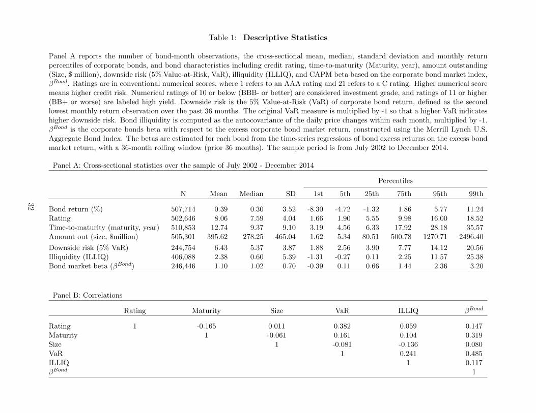
Table 1: Descriptive Statistics

Panel A reports the number of bond-month observations, the cross-sectional mean, median, standard deviation and monthly returnpercentiles of corporate bonds, and bond characteristics including credit rating, time-to-maturity (Maturity, year), amount outstanding(Size, $ million), downside risk (5% Value-at-Risk, VaR), illiquidity (ILLIQ), and CAPM beta based on the corporate bond market index,βBond. Ratings are in conventional numerical scores, where 1 refers to an AAA rating and 21 refers to a C rating. Higher numerical scoremeans higher credit risk. Numerical ratings of 10 or below (BBB- or better) are considered investment grade, and ratings of 11 or higher(BB+ or worse) are labeled high yield. Downside risk is the 5% Value-at-Risk (VaR) of corporate bond return, defined as the secondlowest monthly return observation over the past 36 months. The original VaR measure is multiplied by -1 so that a higher VaR indicateshigher downside risk. Bond illiquidity is computed as the autocovariance of the daily price changes within each month, multiplied by -1.βBond is the corporate bonds beta with respect to the excess corporate bond market return, constructed using the Merrill Lynch U.S.Aggregate Bond Index. The betas are estimated for each bond from the time-series regressions of bond excess returns on the excess bondmarket return, with a 36-month rolling window (prior 36 months). The sample period is from July 2002 to December 2014.

Panel A: Cross-sectional statistics over the sample of July 2002 - December 2014

Percentiles

N Mean Median SD 1st 5th 25th 75th 95th 99th

Bond return (%) 507,714 0.39 0.30 3.52 -8.30 -4.72 -1.32 1.86 5.77 11.24Rating 502,646 8.06 7.59 4.04 1.66 1.90 5.55 9.98 16.00 18.52Time-to-maturity (maturity, year) 510,853 12.74 9.37 9.10 3.19 4.56 6.33 17.92 28.18 35.57Amount out (size, $million) 505,301 395.62 278.25 465.04 1.62 5.34 80.51 500.78 1270.71 2496.40

Downside risk (5% VaR) 244,754 6.43 5.37 3.87 1.88 2.56 3.90 7.77 14.12 20.56Illiquidity (ILLIQ) 406,088 2.38 0.60 5.39 -1.31 -0.27 0.11 2.25 11.57 25.38Bond market beta (βBond) 246,446 1.10 1.02 0.70 -0.39 0.11 0.66 1.44 2.36 3.20

Panel B: Correlations

Rating Maturity Size VaR ILLIQ βBond

Rating 1 -0.165 0.011 0.382 0.059 0.147Maturity 1 -0.061 0.161 0.104 0.319Size 1 -0.081 -0.136 0.080VaR 1 0.241 0.485ILLIQ 1 0.117βBond 1

32

Table 2: Univariate Portfolios of Corporate Bonds Sorted by Downside Risk

Quintile portfolios are formed every month from July 2004 to December 2014 by sorting corpo-rate bonds based on the 5% Value-at-Risk (VaR), defined as the second lowest monthly returnobservation over the past 36 months. The original VaR measure is multiplied by -1. Quintile 1is the portfolio with the lowest VaR, and Quintile 5 is the portfolio with the highest VaR. Tablealso reports the average VaR, the next-month average excess return, and the 7-factor alpha foreach quintile. The last five columns report average portfolio characteristics including bond beta(βBond), illiquidity (ILLIQ), credit rating, time-to-maturity (years), and amount outstanding (size,in $billion) for each quintile. The last row shows the differences in monthly average returns, thedifferences in alphas with respect to the 7-factor models. The 7-factor model includes the excessstock market return (MKT), a size factor (SMB), a book-to-market factor (HML), a momentumfactor (MOM), a liquidity factor (LIQ), plus two bond market factors: the default spread factor(DEF) and the term spread factor (TERM). Average excess returns and alphas are defined inmonthly percentage terms. Newey-West adjusted t-statistics are given in parentheses. ∗, ∗∗, and∗∗∗ indicate the significance at the 10%, 5%, and 1% levels, respectively.

Quintiles Average Average 7-factor Average portfolio characteristics

VaR return alpha βBond ILLIQ Rating Maturity Size

Low VaR 2.90 -0.137 -0.207 0.71 0.78 6.60 8.10 0.53(-1.14) (-2.10)

2 4.18 -0.022 -0.118 0.93 1.35 7.31 10.49 0.51(-0.15) (-1.01)

3 5.39 0.044 -0.066 1.06 1.94 7.79 14.11 0.46(0.25) (-0.50)

4 7.20 0.190 0.076 1.23 2.60 8.72 15.05 0.44(0.89) (0.48)

High VaR 12.47 0.649 0.503 1.49 5.14 11.31 22.23 0.45(2.26) (2.23)

High − Low 0.786∗∗∗ 0.710∗∗∗

Return/Alpha diff. (3.19) (3.85)

33

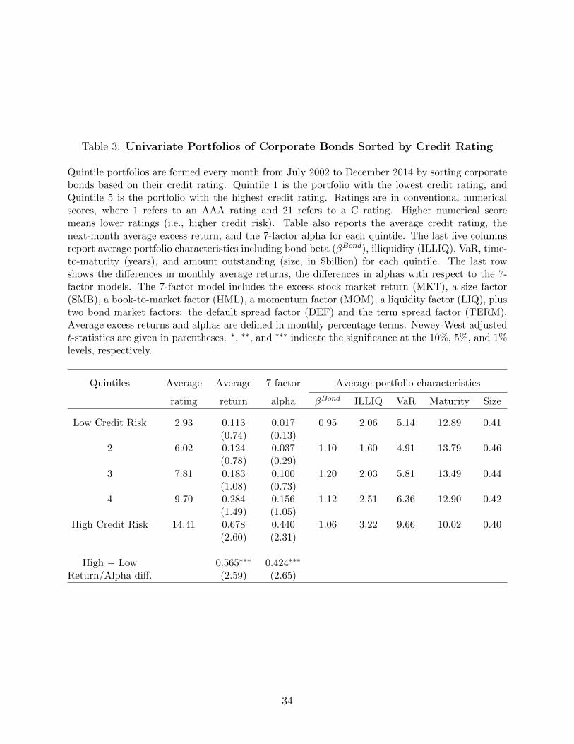
Table 3: Univariate Portfolios of Corporate Bonds Sorted by Credit Rating

Quintile portfolios are formed every month from July 2002 to December 2014 by sorting corporatebonds based on their credit rating. Quintile 1 is the portfolio with the lowest credit rating, andQuintile 5 is the portfolio with the highest credit rating. Ratings are in conventional numericalscores, where 1 refers to an AAA rating and 21 refers to a C rating. Higher numerical scoremeans lower ratings (i.e., higher credit risk). Table also reports the average credit rating, thenext-month average excess return, and the 7-factor alpha for each quintile. The last five columnsreport average portfolio characteristics including bond beta (βBond), illiquidity (ILLIQ), VaR, time-to-maturity (years), and amount outstanding (size, in $billion) for each quintile. The last rowshows the differences in monthly average returns, the differences in alphas with respect to the 7-factor models. The 7-factor model includes the excess stock market return (MKT), a size factor(SMB), a book-to-market factor (HML), a momentum factor (MOM), a liquidity factor (LIQ), plustwo bond market factors: the default spread factor (DEF) and the term spread factor (TERM).Average excess returns and alphas are defined in monthly percentage terms. Newey-West adjustedt-statistics are given in parentheses. ∗, ∗∗, and ∗∗∗ indicate the significance at the 10%, 5%, and 1%levels, respectively.

Quintiles Average Average 7-factor Average portfolio characteristics

rating return alpha βBond ILLIQ VaR Maturity Size

Low Credit Risk 2.93 0.113 0.017 0.95 2.06 5.14 12.89 0.41(0.74) (0.13)

2 6.02 0.124 0.037 1.10 1.60 4.91 13.79 0.46(0.78) (0.29)

3 7.81 0.183 0.100 1.20 2.03 5.81 13.49 0.44(1.08) (0.73)

4 9.70 0.284 0.156 1.12 2.51 6.36 12.90 0.42(1.49) (1.05)

High Credit Risk 14.41 0.678 0.440 1.06 3.22 9.66 10.02 0.40(2.60) (2.31)

High − Low 0.565∗∗∗ 0.424∗∗∗

Return/Alpha diff. (2.59) (2.65)

34

Table 4: Univariate Portfolios of Corporate Bonds Sorted by Illiquidity

Quintile portfolios are formed every month from July 2002 to December 2014 by sorting corporatebonds based on the illiquidity measured, ILLIQ, in Bao, Pan, and Wang (2011). Table alsoreports the average illiquidity, the next-month average excess return, and the 7-factor alpha foreach quintile. The last five columns report average portfolio characteristics including bond beta(βBond), VaR, credit rating, time-to-maturity (years), and amount outstanding (size, in $billion)for each quintile. The last row shows the differences in monthly average returns, the differences inalphas with respect to the 7-factor models. The 7-factor model includes the excess market return(MKT), a size factor (SMB), a book-to-market factor (HML), a momentum factor (MOM), aliquidity factor (LIQ), plus two bond market factors: the default spread factor (DEF) and the termspread factor (TERM). Average excess returns and alphas are defined in monthly percentage terms.Newey-West adjusted t-statistics are given in parentheses. ∗, ∗∗, and ∗∗∗ indicate the significanceat the 10%, 5%, and 1% levels, respectively.

Quintiles Average Average 7-factor Average portfolio characteristics

ILLIQ return alpha βBond VaR Rating Maturity Size

Low ILLIQ -0.16 0.228 0.092 1.05 5.88 8.49 11.29 0.69(1.32) (0.64)

2 0.18 0.020 -0.111 0.99 5.13 8.25 10.11 0.64(0.14) (-0.94)

3 0.61 0.070 -0.067 1.07 5.88 8.33 11.82 0.47(0.45) (-0.54)

4 1.75 0.219 0.072 1.12 6.60 8.11 13.32 0.35(1.19) (0.49)

High ILLIQ 7.85 0.762 0.621 1.21 8.10 8.40 14.76 0.25(2.51) (2.57)

High − Low 0.535∗∗∗ 0.529∗∗∗

Return/Alpha diff. (3.25) (4.13)

35

Table 5: Univariate Portfolios of Corporate Bonds Sorted by Bond Market Beta

Quintile portfolios are formed every month from July 2004 to December 2014 by sorting corporatebonds based on their bond market betas. βBond is the corporate bonds beta with respect to theexcess corporate bond market return, constructed using the Merrill Lynch U.S. Aggregate BondIndex. The betas are estimated for each bond from the time-series regressions of bond excess returnson the excess bond market return with a 36-month rolling window (prior 36 months). Quintile 1 isthe portfolio with the lowest βBond, and Quintile 5 is the portfolio with the highest βBond. Table alsoreports the average βBond, the next-month average excess return, and the 7-factor alpha for eachquintile. The last five columns report average portfolio characteristics including illiquidity (ILLIQ),VaR, credit rating, time-to-maturity (years), and amount outstanding (size, in $billion) for eachquintile. The last row shows the differences in monthly average returns, the differences in alphaswith respect to the 7-factor models. The 7-factor model includes the excess market return (MKT),a size factor (SMB), a book-to-market factor (HML), a momentum factor (MOM), a liquidity factor(LIQ), plus two bond market factors: the default spread factor (DEF) and the term spread factor(TERM). Average excess returns and alphas are defined in monthly percentage terms. Newey-Westadjusted t-statistics are given in parentheses. ∗, ∗∗, and ∗∗∗ indicate the significance at the 10%,5%, and 1% levels, respectively.

Quintiles Average Average 7-factor Average portfolio characteristics

βBond return alpha ILLIQ VaR Rating Maturity Size

Low βBond 0.28 -0.021 -0.119 2.00 5.11 8.60 8.94 0.35(-0.14) (-1.10)

2 0.75 -0.012 -0.113 1.59 5.07 8.09 8.91 0.44(-0.08) (-1.10)

3 1.03 0.077 -0.017 1.68 5.56 7.95 10.30 0.50(0.52) (-0.16)

4 1.35 0.211 0.096 2.01 6.71 8.08 13.33 0.54(1.21) (0.72)

High βBond 2.12 0.568 0.438 3.41 9.73 9.05 18.01 0.53(2.37) (2.03)

High − Low 0.589∗∗∗ 0.557∗∗∗

Return/Alpha diff. (3.48) (3.02)

36

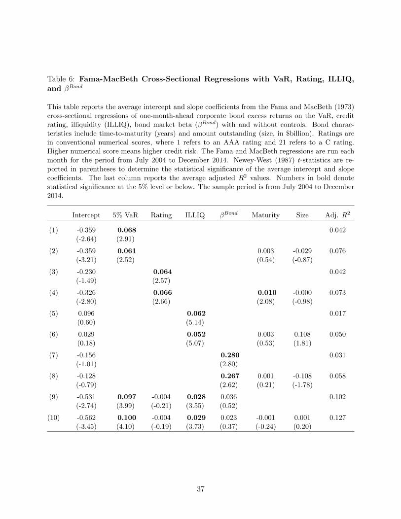
Table 6: Fama-MacBeth Cross-Sectional Regressions with VaR, Rating, ILLIQ,and βBond

This table reports the average intercept and slope coefficients from the Fama and MacBeth (1973)cross-sectional regressions of one-month-ahead corporate bond excess returns on the VaR, creditrating, illiquidity (ILLIQ), bond market beta (βBond) with and without controls. Bond charac-teristics include time-to-maturity (years) and amount outstanding (size, in $billion). Ratings arein conventional numerical scores, where 1 refers to an AAA rating and 21 refers to a C rating.Higher numerical score means higher credit risk. The Fama and MacBeth regressions are run eachmonth for the period from July 2004 to December 2014. Newey-West (1987) t-statistics are re-ported in parentheses to determine the statistical significance of the average intercept and slopecoefficients. The last column reports the average adjusted R2 values. Numbers in bold denotestatistical significance at the 5% level or below. The sample period is from July 2004 to December2014.

Intercept 5% VaR Rating ILLIQ βBond Maturity Size Adj. R2

(1) -0.359 0.068 0.042(-2.64) (2.91)

(2) -0.359 0.061 0.003 -0.029 0.076(-3.21) (2.52) (0.54) (-0.87)

(3) -0.230 0.064 0.042(-1.49) (2.57)

(4) -0.326 0.066 0.010 -0.000 0.073(-2.80) (2.66) (2.08) (-0.98)

(5) 0.096 0.062 0.017(0.60) (5.14)

(6) 0.029 0.052 0.003 0.108 0.050(0.18) (5.07) (0.53) (1.81)

(7) -0.156 0.280 0.031(-1.01) (2.80)

(8) -0.128 0.267 0.001 -0.108 0.058(-0.79) (2.62) (0.21) (-1.78)

(9) -0.531 0.097 -0.004 0.028 0.036 0.102(-2.74) (3.99) (-0.21) (3.55) (0.52)

(10) -0.562 0.100 -0.004 0.029 0.023 -0.001 0.001 0.127(-3.45) (4.10) (-0.19) (3.73) (0.37) (-0.24) (0.20)

37

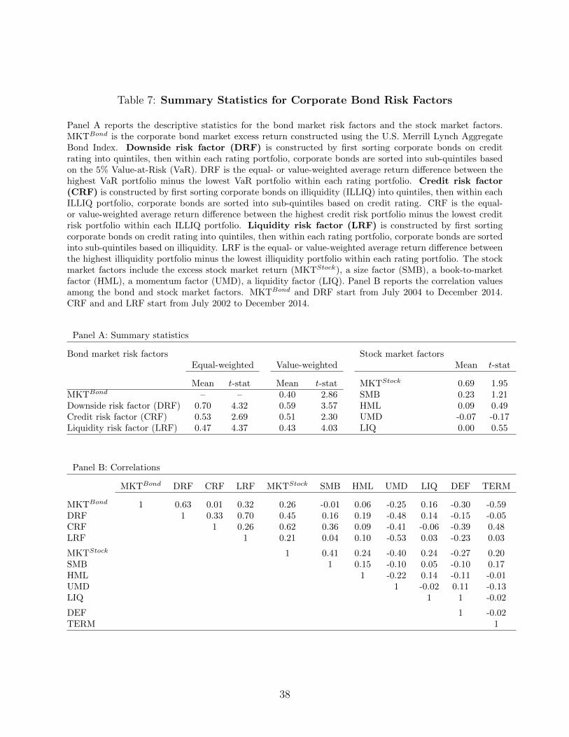
Table 7: Summary Statistics for Corporate Bond Risk Factors

Panel A reports the descriptive statistics for the bond market risk factors and the stock market factors.MKTBond is the corporate bond market excess return constructed using the U.S. Merrill Lynch AggregateBond Index. Downside risk factor (DRF) is constructed by first sorting corporate bonds on creditrating into quintiles, then within each rating portfolio, corporate bonds are sorted into sub-quintiles basedon the 5% Value-at-Risk (VaR). DRF is the equal- or value-weighted average return difference between thehighest VaR portfolio minus the lowest VaR portfolio within each rating portfolio. Credit risk factor(CRF) is constructed by first sorting corporate bonds on illiquidity (ILLIQ) into quintiles, then within eachILLIQ portfolio, corporate bonds are sorted into sub-quintiles based on credit rating. CRF is the equal-or value-weighted average return difference between the highest credit risk portfolio minus the lowest creditrisk portfolio within each ILLIQ portfolio. Liquidity risk factor (LRF) is constructed by first sortingcorporate bonds on credit rating into quintiles, then within each rating portfolio, corporate bonds are sortedinto sub-quintiles based on illiquidity. LRF is the equal- or value-weighted average return difference betweenthe highest illiquidity portfolio minus the lowest illiquidity portfolio within each rating portfolio. The stockmarket factors include the excess stock market return (MKTStock), a size factor (SMB), a book-to-marketfactor (HML), a momentum factor (UMD), a liquidity factor (LIQ). Panel B reports the correlation valuesamong the bond and stock market factors. MKTBond and DRF start from July 2004 to December 2014.CRF and and LRF start from July 2002 to December 2014.

Panel A: Summary statistics

Bond market risk factors Stock market factorsEqual-weighted Value-weighted Mean t-stat

Mean t-stat Mean t-stat MKTStock 0.69 1.95MKTBond – – 0.40 2.86 SMB 0.23 1.21Downside risk factor (DRF) 0.70 4.32 0.59 3.57 HML 0.09 0.49Credit risk factor (CRF) 0.53 2.69 0.51 2.30 UMD -0.07 -0.17Liquidity risk factor (LRF) 0.47 4.37 0.43 4.03 LIQ 0.00 0.55

Panel B: Correlations

MKTBond DRF CRF LRF MKTStock SMB HML UMD LIQ DEF TERM

MKTBond 1 0.63 0.01 0.32 0.26 -0.01 0.06 -0.25 0.16 -0.30 -0.59DRF 1 0.33 0.70 0.45 0.16 0.19 -0.48 0.14 -0.15 -0.05CRF 1 0.26 0.62 0.36 0.09 -0.41 -0.06 -0.39 0.48LRF 1 0.21 0.04 0.10 -0.53 0.03 -0.23 0.03

MKTStock 1 0.41 0.24 -0.40 0.24 -0.27 0.20SMB 1 0.15 -0.10 0.05 -0.10 0.17HML 1 -0.22 0.14 -0.11 -0.01UMD 1 -0.02 0.11 -0.13LIQ 1 1 -0.02

DEF 1 -0.02TERM 1

38

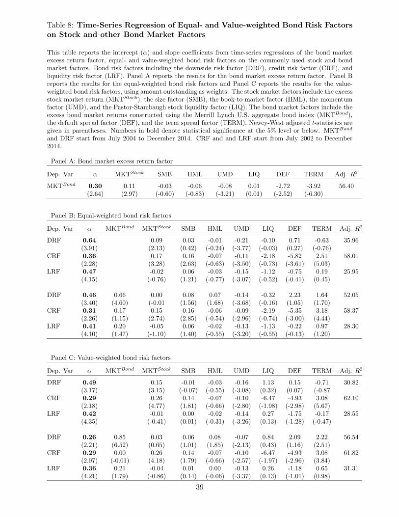
Table 8: Time-Series Regression of Equal- and Value-weighted Bond Risk Factorson Stock and other Bond Market Factors

This table reports the intercept (α) and slope coefficients from time-series regressions of the bond marketexcess return factor, equal- and value-weighted bond risk factors on the commonly used stock and bondmarket factors. Bond risk factors including the downside risk factor (DRF), credit risk factor (CRF), andliquidity risk factor (LRF). Panel A reports the results for the bond market excess return factor. Panel Breports the results for the equal-weighted bond risk factors and Panel C reports the results for the value-weighted bond risk factors, using amount outstanding as weights. The stock market factors include the excessstock market return (MKTStock), the size factor (SMB), the book-to-market factor (HML), the momentumfactor (UMD), and the Pastor-Stambaugh stock liquidity factor (LIQ). The bond market factors include theexcess bond market returns constructed using the Merrill Lynch U.S. aggregate bond index (MKTBond),the default spread factor (DEF), and the term spread factor (TERM). Newey-West adjusted t-statistics aregiven in parentheses. Numbers in bold denote statistical significance at the 5% level or below. MKTBond

and DRF start from July 2004 to December 2014. CRF and and LRF start from July 2002 to December2014.

Panel A: Bond market excess return factor

Dep. Var α MKTStock SMB HML UMD LIQ DEF TERM Adj. R2

MKTBond 0.30 0.11 -0.03 -0.06 -0.08 0.01 -2.72 -3.92 56.40(2.64) (2.97) (-0.60) (-0.83) (-3.21) (0.01) (-2.52) (-6.30)

Panel B: Equal-weighted bond risk factors

Dep. Var α MKTBond MKTStock SMB HML UMD LIQ DEF TERM Adj. R2

DRF 0.64 0.09 0.03 -0.01 -0.21 -0.10 0.71 -0.63 35.96(3.91) (2.13) (0.42) (-0.24) (-3.77) (-0.03) (0.27) (-0.76)

CRF 0.36 0.17 0.16 -0.07 -0.11 -2.18 -5.82 2.51 58.01(2.28) (3.28) (2.63) (-0.63) (-3.50) (-0.73) (-3.61) (5.03)

LRF 0.47 -0.02 0.06 -0.03 -0.15 -1.12 -0.75 0.19 25.95(4.15) (-0.76) (1.21) (-0.77) (-3.07) (-0.52) (-0.41) (0.45)

DRF 0.46 0.66 0.00 0.08 0.07 -0.14 -0.32 2.23 1.64 52.05(3.40) (4.60) (-0.01 (1.56) (1.68) (-3.68) (-0.16) (1.05) (1.70)

CRF 0.31 0.17 0.15 0.16 -0.06 -0.09 -2.19 -5.35 3.18 58.37(2.26) (1.15) (2.74) (2.85) (-0.54) (-2.96) (-0.74) (-3.00) (4.44)

LRF 0.41 0.20 -0.05 0.06 -0.02 -0.13 -1.13 -0.22 0.97 28.30(4.10) (1.47) (-1.10) (1.40) (-0.55) (-3.20) (-0.55) (-0.13) (1.20)

Panel C: Value-weighted bond risk factors

Dep. Var α MKTBond MKTStock SMB HML UMD LIQ DEF TERM Adj. R2

DRF 0.49 0.15 -0.01 -0.03 -0.16 1.13 0.15 -0.71 30.82(3.17) (3.15) (-0.07) (-0.55) (-3.08) (0.32) (0.07) (-0.87

CRF 0.29 0.26 0.14 -0.07 -0.10 -6.47 -4.93 3.08 62.10(2.18) (4.77) (1.81) (-0.66) (-2.80) (-1.98) (-2.98) (5.67)

LRF 0.42 -0.01 0.00 -0.02 -0.14 0.27 -1.75 -0.17 28.55(4.35) (-0.41) (0.01) (-0.31) (-3.26) (0.13) (-1.28) (-0.47)

DRF 0.26 0.85 0.03 0.06 0.08 -0.07 0.84 2.09 2.22 56.54(2.21) (6.52) (0.65) (1.01) (1.85) (-2.13) (0.43) (1.16) (2.51)

CRF 0.29 0.00 0.26 0.14 -0.07 -0.10 -6.47 -4.93 3.08 61.82(2.07) (-0.01) (4.18) (1.79) (-0.66) (-2.57) (-1.97) (-2.96) (3.84)

LRF 0.36 0.21 -0.04 0.01 0.00 -0.13 0.26 -1.18 0.65 31.31(4.21) (1.79) (-0.86) (0.14) (-0.06) (-3.37) (0.13) (-1.01) (0.98)

39

Table 9: Explanatory Power of Alternative Factor Models for Size and Maturity-Sorted Bond Portfolios

The table reports the average adjusted R2 for the time-series regression of the test portfolios’ excess returns on four alternative factor models. PanelA reports the results for the 10 decile bond portfolios sorted on size (amount outstanding). Decile 1 is the portfolio with the smallest size and decile10 is the portfolio with the largest size of corporate bonds. Panel B reports the results for the 10 decile portfolios sorted on time-to-maturity. Decile 1is the portfolio with the shortest time-to-maturity and decile 10 is the portfolio with the longest time-to-maturity of corporate bonds. Panel C reportsthe results for the 25 size and maturity portfolios. The 25 portfolios are formed by independently sorting corporate bonds into 5 by 5 quintile portfoliosbased on size and maturity and then constructed from the intersections of the size and maturity quintiles. Four alternative factor models are considered.Model (1) is the Fama-French (1993) 5-factor model, including the excess stock market return (MKTStock), size factor (SMB), book-to-market factor(HML), default spread factor (DEF), and term spread factor (TERM). Model (2) is the augmented 7-factor model based on the Fama-French (1993)5-factor model, with a momentum factor (MOM) and a Pastor-Stambaugh liquidity factor (LIQ) as additional factors. Model (3) is the bond marketfactor model using the bond market excess returns (MKTBond) as the single factor. Model (4) is the 4-factor model including the bond market excessreturns (MKTBond), the value-weighted downside risk factor (DRF), credit risk factor (CRF), and liquidity risk factor (LRF).

Panel A: 10 size-sorted test portfolios

Model Small 2 3 4 5 6 7 8 9 Large Average R2

(1) 0.27 0.29 0.34 0.52 0.47 0.48 0.49 0.43 0.44 0.39 0.41(2) 0.36 0.40 0.42 0.56 0.54 0.59 0.56 0.50 0.51 0.44 0.49(3) 0.47 0.43 0.50 0.68 0.76 0.75 0.80 0.85 0.85 0.76 0.68(4) 0.58 0.62 0.62 0.86 0.89 0.88 0.89 0.91 0.91 0.87 0.80

Panel B: 10 maturity-sorted test portfolios

Model Short 2 3 4 5 6 7 8 9 Long Average R2

(1) 0.37 0.42 0.47 0.47 0.50 0.47 0.48 0.51 0.51 0.45 0.47(2) 0.43 0.48 0.51 0.50 0.53 0.49 0.50 0.53 0.53 0.47 0.50(3) 0.66 0.69 0.68 0.67 0.77 0.85 0.78 0.77 0.80 0.78 0.75(4) 0.76 0.78 0.81 0.81 0.86 0.89 0.80 0.79 0.79 0.82 0.81

Panel C: Model (1), 25 size- and maturity-sorted portfolios Panel D: Model (2), 25 size- and maturity-sorted portfolios

Short 2 3 4 Long Short 2 3 4 Long

Small 0.25 0.20 0.31 0.33 0.29 Small 0.52 0.42 0.41 0.44 0.422 0.52 0.56 0.50 0.46 0.38 2 0.61 0.66 0.59 0.52 0.463 0.42 0.48 0.50 0.54 0.46 3 0.61 0.64 0.63 0.60 0.504 0.37 0.47 0.44 0.47 0.40 4 0.52 0.63 0.56 0.52 0.44

Large 0.25 0.39 0.41 0.41 0.36 Large 0.40 0.51 0.47 0.45 0.39

Average R2 0.41 Average R2 0.52

Panel E: Model (3), 25 size- and maturity-sorted portfolios Panel F: Model (4), 25 size- and maturity-sorted portfolios

Short 2 3 4 Long Short 2 3 4 Long

Small 0.40 0.26 0.46 0.48 0.49 Small 0.56 0.49 0.54 0.63 0.602 0.46 0.48 0.64 0.70 0.76 2 0.77 0.83 0.85 0.77 0.773 0.59 0.55 0.75 0.79 0.82 3 0.80 0.83 0.91 0.86 0.834 0.68 0.69 0.84 0.84 0.83 4 0.80 0.87 0.91 0.87 0.85

Large 0.63 0.66 0.76 0.74 0.76 Large 0.73 0.84 0.86 0.79 0.85

Average R2 0.64 Average R2 0.78

40

The Cross-section of Expected Corporate Bond Returns

Online Appendix

To save space in the paper, we present some of our findings in the Online Appendix. Table ??

shows the data filtering process for TRACE, Lehman, and NAIC.

1

A.1 Estimation of Stock and Bond Investors’ Risk Aver-

sion Parameter

In this section, we provide empirical evidence to shed light on the differences between stock

and bond investors’ attitudes towards risk (and downside risk). Specifically, we describe the

estimation methodology and then present the estimated risk aversion parameters for the stock

and corporate bond market investors. We use both conditional and unconditional approaches

to estimate the risk aversion parameter.

Following Engle, Lilien and Robins (1987), we use the following GARCH-in-Mean model to

estimate the risk aversion parameter (γ) of the stock and corporate bond market investors:

Rt = α + γ2· σ2

t|t−1 + εt, (A.1)

E(ε2t |Ωt−1

)= σ2

t|t−1 = β0 + β1ε2t−1 + β2σ

2t−1, (A.2)

where Rt denotes the return at time t for the stock or corporate bond market, εt is the in-

formation shock or unexpected news at time t, Ωt−1 is the information set up to time t-1 and

contains the entire history of returns and unexpected news up to time t-1. The conditional

mean of Rt is E(Rt|Ωt−1) = α + γ2· σ2

t|t−1. The current conditional variance of Rt in equation

(A.2) is defined as a function of the last period’s unexpected news or information shocks (as in

Bollerslev (1986)).

Parameters in equations (A.1) and (A.2) are estimated simultaneously using the maximum

likelihood methodology. Assuming that Rt is normally distributed, the conditional density

function for Rt is:

f(Rt; Θ) =1√

2πσ2t|t−1

exp

−1

2

(Rt − µt|t−1σt|t−1

)2

(A.3)

µt|t−1 = α+ γ2·σ2t|t−1 is the conditional mean of Rt, σ

2t|t−1 = β0+β1ε

2t−1+β2σ

2t−1 is the conditional

variance of Rt, and Θ ≡ (α, γ, β0, β1, β2) is the parameter vector. Given the initial values

of εt and σ2t|t−1, the parameters can be estimated by maximizing the log-likelihood function

2

over the sample period. The conditional normal density in equation (A.3) yields the following

conditional log-likelihood function:

LogL(Θ) = −n2

ln(2π)− 1

2

n∑t=1

lnσ2t|t−1 −

1

2

n∑t=1

(Rt − µt|t−1σt|t−1

)2

(A.4)

where n is the number of time-series observations in the Rt sequence. Maximizing equation

(A.4) with respect to the parameter vector yields the maximum likelihood estimates of α, γ, β0,

β1, and β2. Since there is no closed form solution for equation (A.4), we used the Marquardt

algorithm to solve it numerically.

As shown in equations (A.1) and (A.2) , when estimating the risk aversion parameters with

the GARCH-in-Mean model, we account for time-series variations in both the conditional mean

and conditional variance of market returns. Since we use the conditional return distribution

in the estimation of risk aversion parameters, we refer to this as the “conditional approach” in

the paper.

A.2 Experiments with Longer Sample from 1973 to 2014

We collect corporate bond data from six sources: Lehman Brothers fixed income database

(Lehman), Datastream, National Association of Insurance Commissioners database (NAIC),

Bloomberg, the original and enhanced version of the Trade Reporting and Compliance Engine

(TRACE), and Mergent fixed income securities database (FISD). These datasets together com-

prise of the most complete corporate bond data in both the academia and the industry. The

Lehman data are from January 1973 to March 1998; Datastream reports corporate bond infor-

mation from January 1990 to June 2014. Both Lehman and Datastream data provide prices

based on dealer quotes. NAIC reports the transaction information by insurance companies dur-

ing January 1994 to July 2013; Bloomberg provides daily bond prices during January 1997 to

December 2004; and the enhanced TRACE records the transaction of the entire corporate bond

market during July 2002 to March 2014, the original TRACE supplements the bond transaction

data from April 2014 to December 2014. The two datasets, NAIC and TRACE, provide prices

based on the real transactions, whereas other datasets, Lehman, Datastream, and Bloomberg,

3

provides prices based on quotes and matrix calculations.

The quote-based data sets (Lehman and Datastream) provide month-end prices and returns.

NAIC and Bloomberg provide daily prices, and TRACE provides intraday clean prices.

4

Table A.1: Risk Aversion of Stock and Corporate Bond Investors

This table reports the estimated risk aversion parameters for the stock and corporate bond market investors.Three proxies are used for the corporate bond market: the Merrill Lynch aggregate bond index (MKTBond), thevalue-weighted corporate bond index (VW index), and the equal-weighted corporate bond index (EW index).Two proxies are used for the aggregate stock market: the S&P500 index and the value-weighted CRSP indexincluding all stocks trading at NYSE, AMEX, and NASDAQ.

Conditional Approach Unconditional Approach

Corporate Bond Market Risk Aversion Risk Aversion

MKTBond 14.70 16.55VW index 12.58 12.29EW index 12.12 12.63

Stock Market Risk Aversion Risk Aversion

S&P 500 index 5.51 3.50CRSP VW index 7.51 3.71

5

Table A.2: Quintile Portfolios of Corporate Bonds Sorted by VaR Controlling forCredit Rating, Maturity, and Size

Quintile portfolios are formed every month from July 2004 to December 2014 by first sorting corporate bondsbased on credit rating (Panel A), maturity (Panel B) or size (Panel C). Then, within each quintile portfolio,corporate bonds are sorted into sub-quintiles based on their 5% VaR, defined as the second lowest monthlyreturn observation over the past 36 months multiplied by -1. “VaR,1” is the portfolio of corporate bonds withthe lowest VaR within each quintile portfolio and “VaR, 5” is the portfolio of corporate bonds with the highestVaR within each quintile portfolio. Table shows the average excess return and the 7-factor alpha for eachquintile. The last row shows the differences in monthly average returns, the differences in alphas with respectto the 7-factor models. The 7-factor model includes the excess market return (MKT), a size factor (SMB), abook-to-market factor (HML), a momentum factor (MOM), a liquidity factor (ILLIQ), plus two bond marketfactors: the default spread factor (DEF) and the term spread factor (TERM). Average excess returns and alphasare defined in monthly percentage terms. Newey-West adjusted t-statistics are given in parentheses. ∗, ∗∗, and∗∗∗ indicate significance at the 10%, 5%, and 1% levels, respectively.

Panel A: Controlling for credit rating

All bonds Investment-grade Non-investment-grade

Average 7-factor Average 7-factor Average 7-factorreturn alpha return alpha return alpha

VaR,1 -0.131 -0.205 -0.128 -0.188 -0.035 -0.154(-1.26) (-2.47) (-1.10) (-1.85) (-0.14) (-0.96)

VaR,2 -0.043 -0.140 -0.029 -0.108 0.100 -0.065(-0.33) (-1.41) (-0.21) (-0.90) (0.35) (-0.37)

VaR,3 0.061 -0.061 0.044 -0.060 0.208 0.021(0.39) (-0.53) (0.27) (-0.44) (0.62) (0.10)

VaR,4 0.198 0.068 0.141 0.033 0.443 0.246(1.07) (0.49) (0.68) (0.21) (1.10) (1.02)

VaR,5 0.563 0.429 0.377 0.274 0.771 0.576(2.46) (2.24) (1.40) (1.28) (1.64) (2.03)

VaR, 5 − VaR,1 0.694∗∗∗ 0.634∗∗∗ 0.505∗∗∗ 0.463∗∗∗ 0.806∗∗∗ 0.730∗∗∗

Return/Alpha diff. (4.39) (4.23) (2.75) (2.97) (3.09) (3.88)

Panel B: Controlling for maturity

All bonds Short-maturity Medium-maturity Long-maturity

Average 7-factor Average 7-factor Average 7-factor Average 7-factorreturn alpha return alpha return alpha return alpha

VaR,1 -0.119 -0.214 -0.116 -0.158 -0.117 -0.206 -0.053 -0.183(-0.91) (-2.11) (-1.10) (-1.73) (-0.84) (-1.68) (-0.28) (-1.17)

VaR,2 0.003 -0.099 -0.303 -0.365 -0.028 -0.134 0.094 -0.035(0.02) (-0.92) (-1.39) (-1.71) (-0.18) (-1.05) (0.47) (-0.22)

VaR,3 0.056 -0.044 -0.519 -0.583 0.054 -0.049 0.181 0.049(0.37) (-0.38) (-1.48) (-1.78) (0.32) (-0.40) (0.84) (0.28)

VaR,4 0.174 0.067 0.225 0.138 0.121 0.028 0.265 0.119(0.99) (0.52) (0.50) (0.33) (0.51) (0.19) (0.99) (0.60)

VaR,5 0.593 0.447 0.619 0.369 0.531 0.410 0.631 0.443(2.31) (2.25) (1.03) (1.04) (1.41) (1.49) (1.79) (2.08)

VaR, 5 − VaR,1 0.712∗∗∗ 0.661∗∗∗ 0.791 0.576∗∗ 0.648∗∗ 0.615∗∗ 0.684∗∗∗ 0.626∗∗∗

Return/Alpha diff. (3.52) (4.07) (1.48) (1.91) (2.16) (2.58) (2.82) (4.69)

6

Table A.2: (Continued)

Panel C: Controlling for size

All bonds Small bonds Large bonds

Average 7-factor Average 7-factor Average 7-factorreturn alpha return alpha return alpha

VaR,1 -0.117 -0.189 -0.082 -0.171 -0.155 -0.213(-1.10) (-2.06) (-0.64) (-1.55) (-1.33) (-2.06)

VaR,2 -0.014 -0.110 0.044 -0.061 -0.056 -0.147(-0.11) (-1.07) (0.28) (-0.48) (-0.39) (-1.20)

VaR,3 0.085 -0.028 0.078 -0.035 0.046 -0.058(0.54) (-0.24) (0.43) (-0.27) (0.25) (-0.43)

VaR,4 0.177 0.056 0.258 0.125 0.131 -0.005(0.94) (0.38) (0.95) (0.63) (0.57) (-0.03)

VaR,5 0.649 0.502 0.813 0.679 0.488 0.301(2.39) (2.31) (1.89) (2.29) (1.41) (1.26)

VaR, 5 − VaR,1 0.766∗∗∗ 0.692∗∗∗ 0.896∗∗∗ 0.850∗∗∗ 0.643∗∗ 0.514∗∗∗

Return/Alpha diff. (3.58) (3.81) (2.70) (3.54) (2.41) (2.78)

7

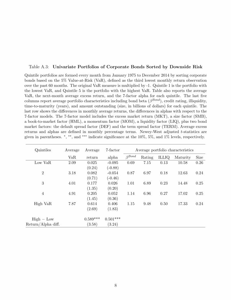
Table A.3: Univariate Portfolios of Corporate Bonds Sorted by Downside Risk

Quintile portfolios are formed every month from January 1975 to December 2014 by sorting corporatebonds based on the 5% Value-at-Risk (VaR), defined as the third lowest monthly return observationover the past 60 months. The original VaR measure is multiplied by -1. Quintile 1 is the portfolio withthe lowest VaR, and Quintile 5 is the portfolio with the highest VaR. Table also reports the averageVaR, the next-month average excess return, and the 7-factor alpha for each quintile. The last fivecolumns report average portfolio characteristics including bond beta (βBond), credit rating, illiquidity,time-to-maturity (years), and amount outstanding (size, in billions of dollars) for each quintile. Thelast row shows the differences in monthly average returns, the differences in alphas with respect to the7-factor models. The 7-factor model includes the excess market return (MKT), a size factor (SMB),a book-to-market factor (HML), a momentum factor (MOM), a liquidity factor (LIQ), plus two bondmarket factors: the default spread factor (DEF) and the term spread factor (TERM). Average excessreturns and alphas are defined in monthly percentage terms. Newey-West adjusted t-statistics aregiven in parentheses. ∗, ∗∗, and ∗∗∗ indicate significance at the 10%, 5%, and 1% levels, respectively.

Quintiles Average Average 7-factor Average portfolio characteristics

VaR return alpha βBond Rating ILLIQ Maturity Size

Low VaR 2.09 0.025 -0.095 0.69 7.15 0.13 10.58 0.26(0.24) (-0.88)

2 3.18 0.082 -0.054 0.87 6.97 0.18 12.63 0.24(0.71) (-0.46)

3 4.01 0.177 0.026 1.01 6.89 0.23 14.48 0.25(1.35) (0.20)

4 4.91 0.205 0.052 1.14 6.96 0.27 17.02 0.25(1.45) (0.36)

High VaR 7.87 0.614 0.406 1.15 9.48 0.50 17.33 0.24(2.69) (1.83)

High − Low 0.589*** 0.501***Return/Alpha diff. (3.58) (3.24)

8

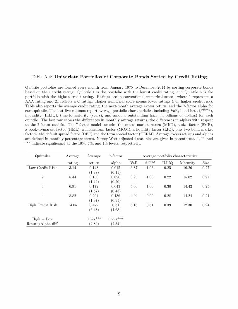
Table A.4: Univariate Portfolios of Corporate Bonds Sorted by Credit Rating

Quintile portfolios are formed every month from January 1975 to December 2014 by sorting corporate bondsbased on their credit rating. Quintile 1 is the portfolio with the lowest credit rating, and Quintile 5 is theportfolio with the highest credit rating. Ratings are in conventional numerical scores, where 1 represents aAAA rating and 21 reflects a C rating. Higher numerical score means lower ratings (i.e., higher credit risk).Table also reports the average credit rating, the next-month average excess return, and the 7-factor alpha foreach quintile. The last five columns report average portfolio characteristics including VaR, bond beta (βBond),illiquidity (ILLIQ), time-to-maturity (years), and amount outstanding (size, in billions of dollars) for eachquintile. The last row shows the differences in monthly average returns, the differences in alphas with respectto the 7-factor models. The 7-factor model includes the excess market return (MKT), a size factor (SMB),a book-to-market factor (HML), a momentum factor (MOM), a liquidity factor (LIQ), plus two bond marketfactors: the default spread factor (DEF) and the term spread factor (TERM). Average excess returns and alphasare defined in monthly percentage terms. Newey-West adjusted t-statistics are given in parentheses. ∗, ∗∗, and∗∗∗ indicate significance at the 10%, 5%, and 1% levels, respectively.

Quintiles Average Average 7-factor Average portfolio characteristics

rating return alpha VaR βBond ILLIQ Maturity SizeLow Credit Risk 3.14 0.148 0.015 3.87 1.03 0.25 16.26 0.27

(1.38) (0.15)2 5.44 0.150 0.020 3.95 1.06 0.22 15.02 0.27

(1.42) (0.20)3 6.91 0.172 0.043 4.03 1.00 0.30 14.42 0.25

(1.67) (0.43)4 8.82 0.204 0.136 4.04 0.99 0.28 14.24 0.24

(1.97) (0.95)High Credit Risk 14.05 0.472 0.31 6.16 0.81 0.39 12.30 0.24

(3.48) (1.68)

High − Low 0.327*** 0.297***Return/Alpha diff. (2.89) (2.34)

9

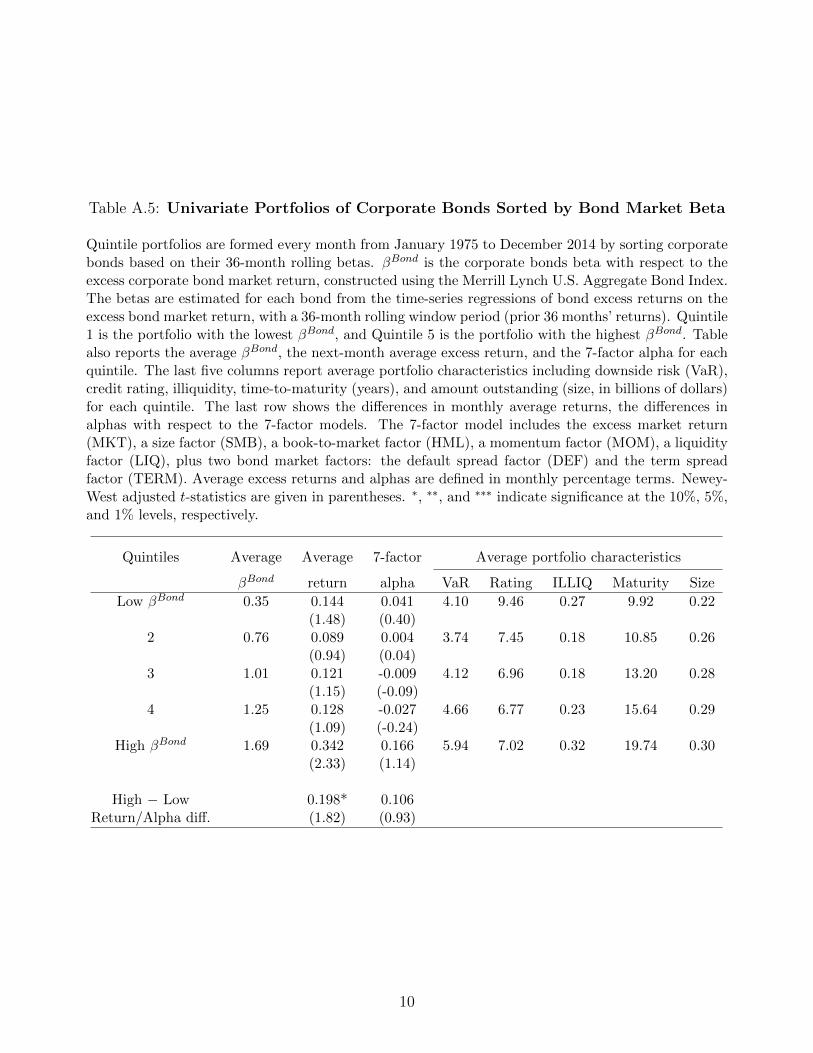
Table A.5: Univariate Portfolios of Corporate Bonds Sorted by Bond Market Beta

Quintile portfolios are formed every month from January 1975 to December 2014 by sorting corporatebonds based on their 36-month rolling betas. βBond is the corporate bonds beta with respect to theexcess corporate bond market return, constructed using the Merrill Lynch U.S. Aggregate Bond Index.The betas are estimated for each bond from the time-series regressions of bond excess returns on theexcess bond market return, with a 36-month rolling window period (prior 36 months’ returns). Quintile1 is the portfolio with the lowest βBond, and Quintile 5 is the portfolio with the highest βBond. Tablealso reports the average βBond, the next-month average excess return, and the 7-factor alpha for eachquintile. The last five columns report average portfolio characteristics including downside risk (VaR),credit rating, illiquidity, time-to-maturity (years), and amount outstanding (size, in billions of dollars)for each quintile. The last row shows the differences in monthly average returns, the differences inalphas with respect to the 7-factor models. The 7-factor model includes the excess market return(MKT), a size factor (SMB), a book-to-market factor (HML), a momentum factor (MOM), a liquidityfactor (LIQ), plus two bond market factors: the default spread factor (DEF) and the term spreadfactor (TERM). Average excess returns and alphas are defined in monthly percentage terms. Newey-West adjusted t-statistics are given in parentheses. ∗, ∗∗, and ∗∗∗ indicate significance at the 10%, 5%,and 1% levels, respectively.

Quintiles Average Average 7-factor Average portfolio characteristics

βBond return alpha VaR Rating ILLIQ Maturity Size

Low βBond 0.35 0.144 0.041 4.10 9.46 0.27 9.92 0.22(1.48) (0.40)

2 0.76 0.089 0.004 3.74 7.45 0.18 10.85 0.26(0.94) (0.04)

3 1.01 0.121 -0.009 4.12 6.96 0.18 13.20 0.28(1.15) (-0.09)

4 1.25 0.128 -0.027 4.66 6.77 0.23 15.64 0.29(1.09) (-0.24)

High βBond 1.69 0.342 0.166 5.94 7.02 0.32 19.74 0.30(2.33) (1.14)

High − Low 0.198* 0.106Return/Alpha diff. (1.82) (0.93)

10