The Standard Deviation of Launch Vehicle Environments

Isam Yunis National Aeronautics and Space Administration, Kennedy Space Center, FL 3.2899

Statistical analysis is used in the development of the launch vehicle environments of acoustics, vibrations, and shock. The standard deviation • of these environments is critical to accurate statistical extrema. However, often very little data exists to define the standard deviation and it is better to use a typical standard deviation than one derived from a few measurements. This paper uses Space Shuttle and expendable launch vehicle flight data to define a typical standard deviation for acoustics and vibrations. The results suggest that 3dB is a conservative and reasonable standard deviation for the source environment and the payload environment.

I. Introduction

Launch vehicle and spacecraft low frequency loads are driven by transients such engine ignitions, engine shut-downs, wind gusts or wind shears, and quasi-static loads. These low frequency loads are developed through the

use of finite element analysis. Other environments are acoustics, random vibration, sine vibration, and shock. These environments are driven by the ascent profile, which includes the events listed in Table 1.

The environments of acoustics, random vibration, sine vibration, and shock are not deterministic. They are also not appropriate for finite element analysis because they typically involve analysis up to thousands of Hertz. The finite element models of launch vehicles and spacecraft cannot be verified above 100 Hz because typically there are already more than 100 modes below 100 Hz. Therefore, rather than being specified as a detailed load, they axe specified globally as a statistically derived environment.

A standard environmental specification is P95/50, which is the level we expect to be greater than 95% of the data with 50% confidence. This is referred to as the Maximum Expected Environment (MPE), or a level that is typically not exceeded. Another standard environment is P99/90, which is described as the Extreme Expected Environment. 1 This is a level that is expected only on the worst day. For both of these definitions, the confidence factor is required because there is very limited flight data from launch vehicles. With an infinite sample size, defining a mean, , and a standard deviation, c, is easy and confidence is 100%. As the sample size gets smaller, confidence in these statistical parameters decreases. It is necessary to consider what confidence we wish to have in the solution.

For launch vehicles, there is typically very limited flight data to perform statistical analysis. Sometimes, there is as little as 1, 2, or 3 flights of data. The following equations shdw that there is. a high cost to be paid for confidence even with 3 data points. It is precisely the confidence cost that is the motivation for this paper.

Table 1. Sources of launch vehicle environments

Acoustics Random \Tibration - Sine Vibration Shock

Lift-off X X _____________ _____ Aerodynamics / Buffet X X __________________ ______ Separation (stage, fairing, spacecraft) _____________ ________________ __________________ x Motor burn / Combustion/POGO ___________ X X - _____

Recall,we seek a limit value (say P95/SO), XL such that:

X L xPUx

* Aerospace Engineer, Launch Services Program, Senior Member AIAA

where Zp is the Normal distribution value for P and P% is the population that must be below the limit value. Note that or o are unknown. All that is available is a small sample of data {x : i=l,2,..,n} and its

associated statistics, 5and s,. n is small (typically <5). 5i and s are approximations for and o, respectively. So we want a factor k such that the value of+ k*s x is greater than i, +Z*o for P% of the samples {x}:

(2)

where P is the confidence we wish to have in the inequality. and s are not equal to and c, respectively. For each sample {x}, and will be different. The sample mean, 5 is normally distributed, N(, o;/n):

z = -

(3)

/

where Z is the normal distribution value for the confidence percentage P and n is the number of points in the sample. Rearranging Equation 3 with a sign change because we want t,>

- z = x +

.vn

Substituting (4) - (1),

X L = + (Z + = + k . a (5)

Equation 5 is an important result and is given in Ref. 1. Equation 5 defines the limit value if the mean is calculated from the data and the standard deviation is known. The value of this is large. Consider if P =5O% and o, is known. Then Z=O and the limit value is given without penalty for small sample size. This lack of penalty occurs only when c is known. This is shown next.

If is not known, the sample standard deviation, s, is calculated from the sample data. This approximation is a random variable with a Chi-squared distribution [2]:

2 (n-l)s(6) cr=

Substituting (5) -, (4),

x = + (Z + s (7)

Equation 6 is of limited use because Z, and Xn-12 cannot be selected independently; it can be seen that Z and X2n-' will be applied to s, which will result in a P higher than desired. Therefore, we approximate the random variable XL from Equation I in terms of the quantities we can calculate:

X L =x+ks

(8)

We want XL? l.t + Zo with confidence P or,

(4)

2

+ks ^i+Z•a

ka /zx+Zp•Ux s x sx

//

zc ____ -+ from (2) s/ s / /cr

=

IXI,//1)

t1 from (4) (9)

V i(n

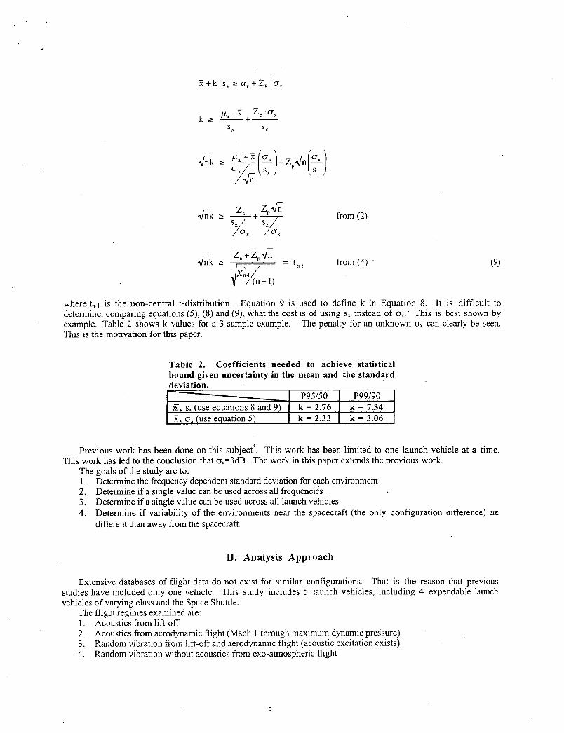
where tn_I is the non-central t-distribution. Equation 9 is used to define k in Equation 8. It is difficult to determine; comparing equations (5), (8) and (9), what the cost is of using s,, instead of o. This is best shown by example. Table 2 shows k values for a 3-sample example. The penalty for an unknown o, can clearly be seen. This is the motivation for this paper.

Table 2. Coefficients needed to achieve statistical bound given uncertainty in the mean and the standard deviation.

P95/SO I P99/90 I (sqtio k=2.76 I k= 7.34 I

, c (use equation 5 k=2.33 I k=3.06 I

Previous work has been done on this subject 3 . This work has been limited to one launch vehicle at a time. This work has led to the conclusion that o =3dB. The work in this paper extends the previous work.

The goals of the study are to: I. Determine the frequency dependent standard deviation for each environment 2. Determine if a single value can be used across all frequencies 3. Determine if a single value can be used across all launch vehicles 4. Determine if variability of the environments near the spacecraft (the only configuration difference) are

different than away from the spacecraft.

H. Analysis Approach

Extensive databases of flight data do not exist for similar configurations. That is the reason that previous studies have included only one vehicle. This study includes 5 launch vehicles, including 4 expendable launch vehicles of varying class and the Space Shuttle.

The flight regimes examined are: 1. Acoustics from lift-off 2. Acoustics from aerodynamic flight (Mach 1 through maximum dynamic pressure) 3. Random vibration from lift-off and aerodynamic flight (acoustic excitation exists) 4. Random vibration without acoustics from exo-atmospheric flight

The data processing approach is as follows: 1. Like configurations were grouped together. This implies that the core vehicle was the same, the number of

solid rocket motors was the same until jettison, the fairing was the same until separation, and the launch pad was the same for lift-off. Only the spacecraft was different.

2. Flight events were identified by the signatures of the data using .the peak value rather than a specific time of flight. This minimizes the effect of different trajectories (loft angle) on the data. However, different maximum dynamic pressures for each flight cannot be avoided. A conservative estimate for the dispersion on maximum dynamic pressure for the same vehicle configuration is E10% around the mean. This

dispersion is expected to cost less than ±1dB of uncertainty in the sound pressure level (SPL) 4 . Therefore, the data was not corrected for flight-to-flight variations in dynamic pressure.

3. Acoustic data was computed as sound pressure level (SPL) and random vibration was computed as power spectral density (PSD).

4. The statistical quantitiesof and s, are computed in the log-space. This is because it has been shown that launch vehicle environments are distributed log-normally [4]. SPL is already in the log-space, so the acoustical statistics were calculated directly. The random vibration PSD's were converted to the log-space before statistics were computed.

5. For random vibrations, the standard deviation was computed across like configurations and normalized by the mean and converted to dB:

- ___ s =101ooi x =10 . s logx (10)

where is the normalized standard deviation in dB and Siogx is the standard deviation of the log of the data. The calculated standard deviation is consistent with the PSD not the log-PSD. Therefore, a standard deviation of 3 dB would be a 2x factor on the PSD. For acoustics, the standard deviation was computed directly and no normalization was applied for the magnitude of the actual SPL. It was seen in the data that the vehicle-to-vehicle variability outweighed the effects of magnitude. The calculated standard deviation shall be added directly to the SPL mean.

III. Results and Conclusions

The results of the study are shown in Figures 1-4. These figures show the variation in standard deviation as a function of frequency. The vehicles cannot be mentioned specifically for proprietary reasons, so they are labeled as Vi -V4. The blue lines represent data that is far from the spacecraft. This is data that should not be influenced by the spacecraft. The red lines are in the vicinity of the spacecraft and are expected to be influenced by the spacecraft differences.

The conclusions from each figure are very similar and simple. These are: 1. A choice of 3 dB is a valid choice for primary environments of lift-off and aerodynamic loading. This

value is not guaranteed to be accurate or conservative, but it represents a reasonable value to use when lacking better information. The conservatism in the use of 3dB is still advantageous in avoiding the costs shown in Table 2.

2. The standard deviation does not appear to have any consistent trend with frequency. There is certainly no increasing or decreasing trend.

3. Any increase in the standard deviation from the spacecraft configuration differences is masked by the flight-to-flight variability. There is a slightly higher bias to the red curves in Figures 1-4, but it is not sufficient to draw a unique conclusion.

4. All launch vehicles have similar environments with similar standard deviations even though the absolute magnitude of the environments and the vehicle configurations vary widely. By looking at one Figure, it may appear that the vehicles have different standard deviations. However, by this conclusion disappears by looking at another measurement or a different time slice.

1

IV. Summan

A study into generalizing the standard deviation of launch vehicle environments has been completed. it has been shown that in the absence of greater than –10 flights of common configuration launch vehicle data, a standard deviation of 3dB relative to the mean is a good choice. This choice will improve and reduce the statistical limit values of P95/50 and P99/90 by reducing the uncertainty in the statistical sample.

—Vi (N=R

—V2 (N=9)

--V3 Ground (N=18)

---V3 Ground (N=10)

-V3 (N=9) ___________

—V4 (N=14) _____

---

- -

Frequency, Hz

Figure 1. Standard deviation of the lift-off acoustic environment of launch vehicles. Red lines are near the spacecraft and should be assumed under the influence of the different spacecraft configurations. Blue lines are away from the spacecraft and are assumed to be comparisons of identical configurations.

5.0

4.5

4.0

0

0 3 3.0

>2.5

02.0

-o C 2 ' Cf.)

1.0

0.5

fl-c)

c

8.0

7.0

6.0 -o 0 0

.4) CD

>

4.0

CD D 3.0 C CD

4J Ci)

1.0

0.0'

1, ', ' C Q c 'i,' ç . ,

Frequency, Hz

Figure 2. Standard deviation of the aerodynamic (transonic/max-q) acoustic environment of launch vehicles. Red lines are near the spacecraft and should be assumed under the influence of the different spacecraft configurations. Blue lines are away from the spacecraft and are assumed to be comparisons of identical configurations.

5 . 0 _______________________ —.—V3 Ground (N=8)

4.5 —V3 Ground (N=12)

---V3 L/O (N=10) 4.0 —V3 L/O (N=10)

—V3 Trans/MaxQ (N=10) -

—V3 Trans/MaxQ (N=10)

10 40 70 100 130 160 190 220 250 280 310 340 370 400

Frequency, Hz

Figure 3. Standard deviation of the random vibration environment of launch vehicles during acoustic events. Red lines are near the spacecraft and should be assumed under the influence of the different spacecraft configurations. Blue lines are away from the spacecraft and are

assumed to be comparisons of identical configurations.

5.0

--V3 (N=10)

________________________________________ —V3 (N=1O) _____ _____-

__________________________________________________--V4 (N=20) --_____

A _ __

0.010 40 70 100 130 160 190 220 250 280 310 340 370 400

Frequency (Hz)

Figure 4. Standard deviation of the random vibration environment of launch vehicles during exo-atmospheric flight. Red lines are near the spacecraft and should be assumed under the influence of the different spacecraft configurations. Blue lines are away from the spacecraft and are assumed to be comparisons of identical configurations.

References

I Department of Defense, "MIL-HDBK-1540C Test Requirements for Launch, Upper Stage, and Space Vehicles", 15 September, 1994.

2 Wirsching. Paul H., Paez, Thomas L, and Ortiz, Keith, Random Vibration Theor y and Practice, John Wiley & Sons, mc, New York, 1995.

3 Pendleton, L.R., and Henrikson, R.L., "Flight-to-Flight Variability in Shock and Vibration Levels Based on Trident I Flight Data", 53rd Symposium on Shock and Vibration, Danvers, Massachusetts, October 26, 1992.

4 Himelblau, H., Kern, D., Maiming, J., Piersol, A., and Rubin, S., "Dynamic Environmental Criteria", NASA-STD-7005, March 13, 2001.

4.5

4.0

3.5

3.0 I

2.5

02.0

1.5

1.0

0.5

.7