
The Sources of Economic Growth The Sources of Economic Growth · The Sources of Economic Growth in...
248
« The Sources of Economic Growth in OECD Countries
Transcript of The Sources of Economic Growth The Sources of Economic Growth · The Sources of Economic Growth in...

ISBN 92-64-19945-411 2003 01 1 P
www.oecd.org
Th
e S
ou
rce
s o
f Ec
on
om
ic G
row
th in
OE
CD
Co
un
tries
«The Sources ofEconomic Growth in OECD Countries
The Sources of Economic Growth in OECD Countries
Growth patterns through the 1990s and into this decade have turned received wisdom on its head. For most of the post-war period OECD countries with relatively low GDP per capita grew faster than richer countries. In the 1990s this pattern broke down. Most notably, the United States, which, already with a relatively high level of GDP percapita among the world’s major economies, drew further ahead of the field from the secondhalf of the 1990s onwards. The growth performance of much of continental Europe remainscomparatively weak and Japan remains mired.
What are the root causes of the divergence in growth across the OECD? How much of it can be attributable to new technology and R&D? What role has macroeconomic policy played? How important is education and training? Are unemployment, labour marketflexibility and product market competition important influences? Do business start-ups helpbring new capital and ideas to markets? How important are the barriers to business start-up and closure? This publication provides a comprehensive overview of these issues and new insights on what drives economic growth in OECD countries.
OECD's books, periodicals and statistical databases are now available via www.SourceOECD.org,our online library.
This book is available to subscribers to the following SourceOECD themes:Science and Information TechnologyGeneral Economics and Future Studies
Ask your librarian for more details of how to access OECD books on line, or write to us at
-:HSTCQE=V^^YZX:

© OECD, 2003.
© Software: 1987-1996, Acrobat is a trademark of ADOBE.
All rights reserved. OECD grants you the right to use one copy of this Program for your personal use only.Unauthorised reproduction, lending, hiring, transmission or distribution of any data or software isprohibited. You must treat the Program and associated materials and any elements thereof like any othercopyrighted material.
All requests should be made to:
Head of Publications Service,OECD Publications Service,2, rue André-Pascal, 75775 Paris Cedex 16, France.

The Sources of Economic Growth in OECD Countries
ORGANISATION FOR ECONOMIC CO-OPERATION AND DEVELOPMENT

ORGANISATION FOR ECONOMIC CO-OPERATIONAND DEVELOPMENT
Pursuant to Article 1 of the Convention signed in Paris on 14th December 1960,and which came into force on 30th September 1961, the Organisation for Economic
Co-operation and Development (OECD) shall promote policies designed:
– to achieve the highest sustainable economic growth and employment and arising standard of living in member countries, while maintaining financialstability, and thus to contribute to the development of the world economy;
– to contribute to sound economic expansion in member as well as non-membercountries in the process of economic development; and
– to contribute to the expansion of world trade on a multilateral, non-discriminatorybasis in accordance with international obligations.
The original member countries of the OECD are Austria, Belgium, Canada,
Denmark, France, Germany, Greece, Iceland, Ireland, Italy, Luxembourg, theNetherlands, Norway, Portugal, Spain, Sweden, Switzerland, Turkey, the UnitedKingdom and the United States. The following countries became memberssubsequently through accession at the dates indicated hereafter: Japan(28th April 1964), Finland (28th January 1969), Australia (7th June 1971), New Zealand(29th May 1973), Mexico (18th May 1994), the Czech Republic (21st December 1995),Hungary (7th May 1996), Poland (22nd November 1996), Korea (12th December 1996)and the Slovak Republic (14th December 2000). The Commission of the EuropeanCommunities takes part in the work of the OECD (Article 13 of the OECD Convention).
Publié en français sous le titre :
Les sources de la croissance économique dans les pays de l’OCDE
© OECD 2003
Permission to reproduce a portion of this work for non-commercial purposes or classroom use should be obtained through
the Centre français d’exploitation du droit de copie (CFC), 20, rue des Grands-Augustins, 75006 Paris, France, tel. (33-1) 44 07 47 70,fax (33-1) 46 34 67 19, for every country except the United States. In the United States permission should be obtained
through the Copyright Clearance Center, Customer Service, (508)750-8400, 222 Rosewood Drive, Danvers, MA 01923 USA,or CCC Online: www.copyright.com. All other applications for permission to reproduce or translate all or part of this book
should be made to OECD Publications, 2, rue André-Pascal, 75775 Paris Cedex 16, France.
FOREWORD
Foreword
In the last decade, per capita growth rates in OECD countries have ceased to
converge. Productivity has accelerated in some of the most affluent economies, most
notably the United States, and slowed down substantially in others, such as
continental Europe and Japan, while signs of what has been named a “New Economy”,
driven by the upsurge of new technologies, have emerged. To understand some of the
reasons behind these developments, and more generally to answer the request
advanced in 1999 by OECD Ministers “to analyse the causes underlying differences in
growth performance … and identify factors, institutions and policies that could
enhance long-term growth prospects”, the Organisation has produced a remarkable
amount of comparative analysis and new research. While a short synthesis of the
main findings and policy conclusions from this project has been published in a report
to Ministers, The New Economy: Beyond the Hype, a single volume which pulls
together the background research carried out by the Economics Department and other
OECD Directorates has been lacking. This book aims to fill that gap.
What makes some countries seemingly able to thrive on new technological
opportunities while others are held back? This book confronts this issue head on. It not
only takes a long-term view on aggregate economic growth rates of OECD countries
and examines their main influences and policy drivers, but also investigates how
growth is determined at the industry and firm level. I think it can make the modest, but
important, claim of moving us one step further towards a clearer image of what
matters for growth and where policy should focus.
One of the most important lessons to emerge from this work is that policies that
ensure stable macroeconomic conditions are important for growth, as high and
variable inflation depresses investment and excessive tax burdens distort proper
resource allocation. Also, the importance of capital – in the broadest sense – is
reaffirmed; there are high returns not only to physical capital accumulation but also to
investment in education and R&D. In addition, institutional structures and policy
settings that favour competition and flexibility in capital and labour markets, the
development of new technologies and the diffusion of innovations and technological
change also make a key difference to growth prospects. In particular, many of our
countries need more competitive product markets; labour markets that adjust better
and more rapidly to shocks, both demographic and technological; and, financial
systems that are able to direct capital flows, for given risks, towards projects with the
highest returns.
THE SOURCES OF ECONOMIC GROWTH IN THE OECD COUNTRIES – ISBN 92-64-19945-4 – © OECD 2003 3
FOREWORD
This book also reminds us that the “new economy” is in part an old story. The
upsurge in the use of information and communication technologies in the second half
of the nineties has been spectacular in some countries through high levels of
investment and utilisation. The evidence shows that this has clearly boosted efficiency
and, when properly accounting for quality changes, has produced substantial capital
deepening and higher growth rates, even if, so far, evidence of there being extra
impacts from this wave of new capital due to network effects remains weak. The recent
negative stock market and corporate developments are unlikely to change this
assessment. But the new economy has also served to remind us how difficult it is to
evaluate growth when new technologies are being rapidly developed and implemented,
accompanied by swings of optimism and pessimism about the economic value of these
advances.
To be sure, economic growth is neither a mechanical nor a smooth process.
Institutions and regulations play a crucial role in determining the path of growth. But
if the “rules of the game” start being perceived as blurred and non-transparent, capital
deepening and productivity enhancements may suffer. More generally, macroeconomic
stability and well-functioning markets cannot be taken for granted even where they
have best served the cause of economic growth in the last decades. Furthermore,
contrary to simplistic beliefs, regulatory reforms are not the same as unconstrained
deregulation; enhanced competition does not mean uncontrolled laisser-faire; and the
reduction of excessive employment protection does not inevitably imply widespread
job-insecurity. The quest for the most appropriate conditions to foster investment
opportunities and economic growth needs to focus on enhancing market efficiency and
innovation, promoting the accumulation of knowledge and increasing the diffusion of
new technologies. The OECD’s on-going monitoring of the developments and impacts
of these new technologies will, I hope, help bring us closer to an understanding of the
real nature of the “new economy” and where it is heading.
These messages on how policymakers can help growth are perhaps not
completely new but the evidence in this volume gives us reason to believe they should
be made more forcefully so as to encourage a thorough assessment of institutions and
structural policies in the OECD countries.
Ignazio Visco
OECD Chief Economist, 1997-2002
4 THE SOURCES OF ECONOMIC GROWTH IN THE OECD COUNTRIES – ISBN 92-64-19945-4 – © OECD 2003

ACKNOWLEDGEMENTS
Acknowledgements
The OECD is indebted to its former chief economist, Ignazio Visco, for his
inspiration for this publication and for his subsequent editorial advice.
The principal author and editor of this book was Stefano Scarpetta, senior
economist at the OECD (currently on loan to the World Bank as the labour market
advisor). Other members of the drafting and editing team included Romain Duval,
Philip Hemmings, Willi Leibritz and Nick Vanston. The book benefited from extensive
comments from Michael Feiner and Jorgen Elmeskov. Preliminary versions of the
different chapters were presented at meetings of the Economic Policy Committee and its
Working Party No. 1. Participants to these meetings provided valuable comments.
Statistical assistance was provided by Catherine Chapuis-Grabiner.
A large number of researchers were involved in the background research to this book.
Among OECD staff, special thanks are due to Sanghoon Ahn, Andrea Bassanini, Dirk Pilat,
Paul Schreyer, Thierry Tressel and Jaejoon Woo. The project also included many
researchers whose governments and institutions allowed them to spend considerable
time working on the firm-level project. A special thanks is due to Eric Bartelsman (Free
University of Amsterdam) for helping co-ordinate the project.
Finally, many thanks are also due to Irene Sinha, Catherine Candea and Rory Clarke
for their help in getting the publication to print and for helping with promotion and
marketing.
THE SOURCES OF ECONOMIC GROWTH IN THE OECD COUNTRIES – ISBN 92-64-19945-4 – © OECD 2003 5
TABLE OF CONTENTS
Table of Contents
Summary and Policy Conclusions . . . . . . . . . . . . . . . . . . . . . . . . . . . . . . 13
Chapter 1. Economic Growth: the Aggregate Evidence . . . . . . . . . . . . 27
Introduction . . . . . . . . . . . . . . . . . . . . . . . . . . . . . . . . . . . . . . . . 28
1.1. Recent cross-country growth patterns . . . . . . . . . . . . . . . . . . 28
1.2. The role of skills and labour utilisation in labour
productivity growth . . . . . . . . . . . . . . . . . . . . . . . . . . . . . . . . . . 37
1.3. The role of information and communication technology . . 38
1.4. Multi-factor productivity growth . . . . . . . . . . . . . . . . . . . . . . . 45
1.5. Concluding remarks. . . . . . . . . . . . . . . . . . . . . . . . . . . . . . . . . . 51
Chapter 2. Policy Settings, Institutions and Aggregate Economic Growth: a Cross-country Analysis . . . . . . . . . . . . . . . . . . . . 55
Introduction . . . . . . . . . . . . . . . . . . . . . . . . . . . . . . . . . . . . . . . . 56
2.1. An overview of policy influences on economic growth . . . . 57
2.2. Econometric evidence on the links between investment,
policy settings and growth . . . . . . . . . . . . . . . . . . . . . . . . . . . . 71
2.3. Assessing the long-run effects of policy and institutional
changes on GDP per capita . . . . . . . . . . . . . . . . . . . . . . . . . . . . 87
2.4. Concluding remarks. . . . . . . . . . . . . . . . . . . . . . . . . . . . . . . . . . 89
Chapter 3. What Drives Productivity Growth at the Industry Level? 95
Introduction . . . . . . . . . . . . . . . . . . . . . . . . . . . . . . . . . . . . . . . . 96
3.1. Within-industry growth and reallocation of resources
across industries . . . . . . . . . . . . . . . . . . . . . . . . . . . . . . . . . . . . 96
3.2. An overview of the potential influences of policies
and institutions on productivity . . . . . . . . . . . . . . . . . . . . . . . 99
3.3. Empirical analysis . . . . . . . . . . . . . . . . . . . . . . . . . . . . . . . . . . . 103
3.4. Concluding remarks. . . . . . . . . . . . . . . . . . . . . . . . . . . . . . . . . . 120
THE SOURCES OF ECONOMIC GROWTH IN THE OECD COUNTRIES – ISBN 92-64-19945-4 – © OECD 2003 7
TABLE OF CONTENTS
Chapter 4. Firm Dynamics, Productivity and Policy Settings . . . . . . . 127
Introduction . . . . . . . . . . . . . . . . . . . . . . . . . . . . . . . . . . . . . . . . 1284.1. What lies behind within-industry productivity growth?
Reallocation of resources versus within-firm growth . . . . . . 1304.2. The entry and exit of firms. . . . . . . . . . . . . . . . . . . . . . . . . . . . 1394.3. Which firms survive and which expand?. . . . . . . . . . . . . . . . 143
4.4. Regulations, institutions and firm entry: empirical analysis 1464.5. Concluding remarks. . . . . . . . . . . . . . . . . . . . . . . . . . . . . . . . . . 155
Annex 1. Macroeconomic indicators of economic growth . . . . . . . . . . 159Annex 2. The policy-and-institutions augmented growth model . . . . 177
Annex 3. Methodological details on the empirical analysis of industry multi-factor productivity . . . . . . . . . . . . . . . . . . . 180
Annex 4. Details on firm-level data . . . . . . . . . . . . . . . . . . . . . . . . . . . . . 183
Annex 5. Basic data and sources . . . . . . . . . . . . . . . . . . . . . . . . . . . . . . . 208
Bibliography . . . . . . . . . . . . . . . . . . . . . . . . . . . . . . . . . . . . . . . . . . . . . . . . . 235
List of boxes1.1. Trend series: the extended Hodrick-Prescott filter . . . . . . . . . . . 301.2. Estimating changes in the quality of factor inputs:
the example of the labour input . . . . . . . . . . . . . . . . . . . . . . . . . . 39
1.3. Price measurement issues in ICT goods. . . . . . . . . . . . . . . . . . . . 431.4. Measures of multi-factor productivity (MFP) . . . . . . . . . . . . . . . . 48
1.5. Problems associated with assessing spillover effects in ICT-using sectors . . . . . . . . . . . . . . . . . . . . . . . . . . . . . . . . . . . . . 52
2.1. Policy settings and growth: what does theory suggest?. . . . . . . 582.2. The estimation technique . . . . . . . . . . . . . . . . . . . . . . . . . . . . . . . 752.3. Description of the variables used in the empirical analysis . . . 77
2.4. Consistency of results with different growth models . . . . . . . . 803.1. The theoretical links between product market competition
and productivity. . . . . . . . . . . . . . . . . . . . . . . . . . . . . . . . . . . . . . . . 1013.2. The estimated multi-factor productivity equation. . . . . . . . . . . 1053.3. Indicators of the stringency of product market regulations
and employment protection legislation . . . . . . . . . . . . . . . . . . . . 1103.4. A taxonomy of manufacturing industries according to
their technology regimes . . . . . . . . . . . . . . . . . . . . . . . . . . . . . . . . 1164.1. “Creative Destruction”, firm dynamics and economic growth . 129
4.2. Building up a consistent international dataset: the OECD firm-level study . . . . . . . . . . . . . . . . . . . . . . . . . . . . . . . 131
4.3. The decomposition of productivity growth . . . . . . . . . . . . . . . . . 133
4.4. The size of firms across sectors and countries . . . . . . . . . . . . . . 148
8 THE SOURCES OF ECONOMIC GROWTH IN THE OECD COUNTRIES – ISBN 92-64-19945-4 – © OECD 2003
TABLE OF CONTENTS
List of tables1.1. Uneven growth of GDP across the OECD countries. . . . . . . . . . . 32
1.2. Rapid labour productivity growth in ICT industries sectors, 1999 42
1.3. The role of embodied and disembodied components
of multi-factor productivity growth . . . . . . . . . . . . . . . . . . . . . . . 50
2.1. The long-term improvement in the level of education
of the population . . . . . . . . . . . . . . . . . . . . . . . . . . . . . . . . . . . . . . . 62
2.2. Total government outlays and “productive” government
spending as a share of total spending . . . . . . . . . . . . . . . . . . . . . 69
2.3. The role of convergence and accumulation of capital for growth:
summary of regression results . . . . . . . . . . . . . . . . . . . . . . . . . . . 79
2.4. Macro-policy influences on growth. . . . . . . . . . . . . . . . . . . . . . . . 82
2.5. The influence of financial market developments on growth . . 84
2.6. Growth regressions including R&D intensity variables . . . . . . . 85
2.7. Investment regressions. . . . . . . . . . . . . . . . . . . . . . . . . . . . . . . . . . 86
2.8. Estimated impact of changes in institutional
or policy factors on output per capita. . . . . . . . . . . . . . . . . . . . . . 88
3.1. Productivity regressions: the role of regulations
and institutions . . . . . . . . . . . . . . . . . . . . . . . . . . . . . . . . . . . . . . . . 107
3.2. Productivity regressions: the role of R&D, market structure
and regulatory settings – Manufacturing . . . . . . . . . . . . . . . . . . . 114
3.3. The effects of policies and institutions on R&D intensity . . . . . 118
3.4. Estimated effects of employment protection on R&D intensity 120
4.1. Analysis of productivity components across industries
of manufacturing and services . . . . . . . . . . . . . . . . . . . . . . . . . . . 135
4.2. Strong correlation between entry and exit rates, 1989-1994 . . . 141
4.3. Differences in entry rates across industries do not persist
over time . . . . . . . . . . . . . . . . . . . . . . . . . . . . . . . . . . . . . . . . . . . . . . 143
4.4. Variability of entry and hazard rates across industries, 1989-1994 145
4.5. Entry rate regressions: baseline specification . . . . . . . . . . . . . . . 151
4.6. Entry rate regressions: the role of regulations and institutions . . 152
A1.1. Actual GDP growth in the OECD area, by sub-period . . . . . . . . . 166
A1.2. Actual GDP per capita growth in the OECD area, by sub-period 167
A1.3. Actual GDP per person employed in the OECD area,
by sub-period . . . . . . . . . . . . . . . . . . . . . . . . . . . . . . . . . . . . . . . . . . 168
A1.4. Trend GDP growth in the OECD area, by sub-period. . . . . . . . . . 169
A1.5. Trend GDP per capita growth in the OECD area, by sub-period 170
A1.6. Trend GDP per person employed in the OECD area,
by sub-period . . . . . . . . . . . . . . . . . . . . . . . . . . . . . . . . . . . . . . . . . . 171
THE SOURCES OF ECONOMIC GROWTH IN THE OECD COUNTRIES – ISBN 92-64-19945-4 – © OECD 2003 9
TABLE OF CONTENTS
A1.7. Trend GDP growth in the OECD area, by sub-period,
business sector. . . . . . . . . . . . . . . . . . . . . . . . . . . . . . . . . . . . . . . . . 172
A1.8. Trend GDP per person employed in the OECD area,
by sub-period, business sector. . . . . . . . . . . . . . . . . . . . . . . . . . . . 173
A1.9. Sensitivity analysis: MFP growth estimates (adjusted
for hours worked), 1980-2000. . . . . . . . . . . . . . . . . . . . . . . . . . . . . 174
A4.1. The STAN industry list (based on ISIC Rev. 3) . . . . . . . . . . . . . . . 185
A4.2. Labour productivity decompositions
Finland, average period: 1987-1992 . . . . . . . . . . . . . . . . . . . . . . . . 191
A4.2. Labour productivity decompositions (cont.)
Finland, average period: 1989-1994 . . . . . . . . . . . . . . . . . . . . . . . . 192
A4.3. Labour productivity decompositions
France, average period: 1987-1992. . . . . . . . . . . . . . . . . . . . . . . . . 193
A4.4. Labour productivity decompositions
Italy, average period: 1987-1992 . . . . . . . . . . . . . . . . . . . . . . . . . . . 194
A4.4. Labour productivity decompositions (cont.)
Italy, average period: 1992-1997 . . . . . . . . . . . . . . . . . . . . . . . . . . . 195
A4.5. Labour productivity decompositions
Netherlands, average period: 1987-1992. . . . . . . . . . . . . . . . . . . . 196
A4.5. Labour productivity decompositions (cont.)
Netherlands, average period: 1992-1997. . . . . . . . . . . . . . . . . . . . 197
A4.6. Labour productivity decompositions
Portugal, average period: 1987-1992 . . . . . . . . . . . . . . . . . . . . . . . 198
A4.6. Labour productivity decompositions (cont.)
Portugal, average period: 1992-1997 . . . . . . . . . . . . . . . . . . . . . . . 199
A4.7. Labour productivity decompositions
United Kingdom, average period: 1987-1992 . . . . . . . . . . . . . . . . 200
A4.7. Labour productivity decompositions (cont.)
United Kingdom, average period: 1992-1997 . . . . . . . . . . . . . . . . 201
A4.8. Labour productivity decompositions
United States, average period: 1987-1992. . . . . . . . . . . . . . . . . . . 202
A4.8. Labour productivity decompositions (cont.)
United States, average period: 1992-1997 . . . . . . . . . . . . . . . . . . . 203
A5.1. Basic data for international comparaison of income
and productivity, 2000 . . . . . . . . . . . . . . . . . . . . . . . . . . . . . . . . . . . 209
A5.2. Average hours worked annually, 1980-2000. . . . . . . . . . . . . . . . . 212
A5.3. Average years of education of the working age population,
1971-1998 . . . . . . . . . . . . . . . . . . . . . . . . . . . . . . . . . . . . . . . . . . . . . 216
10 THE SOURCES OF ECONOMIC GROWTH IN THE OECD COUNTRIES – ISBN 92-64-19945-4 – © OECD 2003
TABLE OF CONTENTS
A5.4. Industries used in the productivity analysis and classification
according to the technology regime (manufacturing) . . . . . . . . 217
A5.5. Coverage of multi-factor productivity data . . . . . . . . . . . . . . . . . 218
A5.6. Industry-specific product market regulation:
coverage and sources . . . . . . . . . . . . . . . . . . . . . . . . . . . . . . . . . . . 223
A5.7. Description of data used in analysis of firm demographics . . . 226
A5.8. Description of data used in productivity decompositions. . . . . 231
List of figures
1.1. Large differentials in GDP per capita . . . . . . . . . . . . . . . . . . . . . . . . . 34
1.2. The driving forces of GDP per capita growth . . . . . . . . . . . . . . . . . . 36
1.3. Enhancements in human capital contribute to labour
productivity growth . . . . . . . . . . . . . . . . . . . . . . . . . . . . . . . . . . . . . . . 38
1.4. Disparities in human capital enhancement amongst employed
workers and the working age population . . . . . . . . . . . . . . . . . . . . . 40
1.5. Different size of the ICT industry across OECD countries . . . . . . . 41
1.6. The rise in ICT investment . . . . . . . . . . . . . . . . . . . . . . . . . . . . . . . . . 45
1.7. ICT capital has boosted GDP growth . . . . . . . . . . . . . . . . . . . . . . . . . 46
1.8. Multi-factor productivity growth accelerated in some countries . 51
2.1. Business-sector investment share has typically increased . . . . . . 61
2.2. Business R&D has risen, government R&D budgets have declined 63
2.3. The link between the level of inflation and economic growth . . . 65
2.4. Changes in the variability of inflation and growth
between the 1980s and 1990s . . . . . . . . . . . . . . . . . . . . . . . . . . . . . . . 66
2.5. Total government expenditure and liabilities as a percentage
of GDP. . . . . . . . . . . . . . . . . . . . . . . . . . . . . . . . . . . . . . . . . . . . . . . . . . . 68
2.6. Greater exposure of several OECD countries to foreign trade . . . . 70
2.7. Significant developments in financial systems . . . . . . . . . . . . . . . . 72
3.1. Decomposition of aggregate labour productivity growth into
intra-sectoral productivity growth and inter-sectoral
employment shifts . . . . . . . . . . . . . . . . . . . . . . . . . . . . . . . . . . . . . . . . 98
3.2. The contribution of ICT-related industries to labour productivity
growth . . . . . . . . . . . . . . . . . . . . . . . . . . . . . . . . . . . . . . . . . . . . . . . . . . 100
4.1. Decomposition of labour productivity growth in manufacturing . 134
4.2. Decomposition of labour productivity growth in selected
service sectors. . . . . . . . . . . . . . . . . . . . . . . . . . . . . . . . . . . . . . . . . . . . 137
4.3. Decomposition of multi-factor productivity growth
in manufacturing . . . . . . . . . . . . . . . . . . . . . . . . . . . . . . . . . . . . . . . . . 138
4.4. High firm turnover rates in OECD countries . . . . . . . . . . . . . . . . . . 140
THE SOURCES OF ECONOMIC GROWTH IN THE OECD COUNTRIES – ISBN 92-64-19945-4 – © OECD 2003 11

TABLE OF CONTENTS
4.5. Estimated entry rates with control for industry composition . . . . 141
4.6. Significant differences in entry rates across industries . . . . . . . . . 142
4.7. Strong market selection amongst new entrants . . . . . . . . . . . . . . . 144
4.8. Entrant and exiting firms are relatively small . . . . . . . . . . . . . . . . . 147
4.9. Different post-entry growth patterns across the OECD countries 149
A4.1. The evolution of labour productivity and its components,
total manufacturing . . . . . . . . . . . . . . . . . . . . . . . . . . . . . . . . . . . . . 204
A4.2. Decomposition of multi-factor productivity growth,
total manufacturing . . . . . . . . . . . . . . . . . . . . . . . . . . . . . . . . . . . . . 206
12 THE SOURCES OF ECONOMIC GROWTH IN THE OECD COUNTRIES – ISBN 92-64-19945-4 – © OECD 2003

ISBN 92-64-19945-4
The Sources of Economic Growth in the OECD Countries© OECD 2003
Summary and Policy Conclusions
THE SOURCES OF ECONOMIC GROWTH IN THE OECD COUNTRIES – ISBN 92-64-19945-4 – © OECD 2003 13
SUMMARY AND POLICY CONCLUSIONS
Strong economic growth in some OECD countries over the 1990s, mostnotably in the United States, led many commentators to speculate that a “neweconomy” had emerged, largely driven by the spread of information andcommunication technology (ICT). In particular, economic performance in theUnited States included a combination of strong output and productivitygrowth, together with falling unemployment and low inflation. These patternswere all the more surprising for a country already at the technology frontier in
many industries, and had no similar counterpart in other affluent OECDeconomies. Indeed, over the 1990s, large continental European countries, andJapan, experienced slow economic growth and rising, or persistently highunemployment.
Two main features were put forward as characterising this new economyphase. First, ICT may have led to an upward shift in the growth path in those
economies where it was most widespread. Indeed, some of the fast-growingcountries of the 1990s (such as the United States and, more recently, Finland)developed a sizeable ICT-production industry, whose output and productivitysoared, increasingly contributing to aggregate growth. Yet, growth alsoaccelerated in some countries without an ICT-production industry(e.g. Australia and the Netherlands) and the sizeable ICT sector in Japan didnot prevent it from experiencing a significant deceleration. But ICT may alsohave influenced growth via other channels. In particular, greater use of ICTequipment in the production process of other industries enhanced aggregategrowth in some of the countries lacking an ICT-production industry(e.g. Australia).
It could be argued that the interest of policymakers and analysts in theimpact of ICT on economic growth should have evaporated along with thenew-economy hype and the over-valuation of ICT-related stocks. Yet, behindthe falling stock prices, IC-related technologies continue to have the potentialto affect the quality and variety of goods and services, as well as the costs oftransaction between many economic agents. In addition, the use of ICT maybe increasing the efficiency of innovation, further contributing to long-term
growth potential.
Of course, the spread of ICT was not the only factor shaping the economiclandscape of the OECD economies in the 1990s. It was a period characterisedby sound macroeconomic policy settings, as well as structural reforms inproduct, labour and financial markets in several countries. The pace and
14 THE SOURCES OF ECONOMIC GROWTH IN THE OECD COUNTRIES – ISBN 92-64-19945-4 – © OECD 2003
SUMMARY AND POLICY CONCLUSIONS
depth of structural reforms differed significantly across countries, with some
(generally small) countries (e.g., Australia, Ireland, Netherlands, New Zealand)pursuing major changes, while others (including several large economies)were being somewhat more hesitant, particularly with reforms in product andespecially the labour markets.
The book presents an in-depth reflection on what has been drivingeconomic growth in OECD countries over the most recent decades. What do
recent estimates say about the impact of the spread of ICT on growth? Whyhave some economies been able to harness the potential of this technologybetter than others? How and how much, does government activity contributeto long-term growth, not least by creating suitable framework conditions forinnovation and the adoption of new technologies? What policies (macro aswell as structural) should be advocated for sustainable long-term growth?What lessons do policy practices in individual countries have for others?
The analysis is based on a newly developed set of indicators of policy andregulations in different markets to disentangle the effect of the various factorsat work, and to examine how they affect specific sectors of the economy.Different tools are used to exploit this information and assess the sources ofeconomic growth. They range from growth-accounting methods, offering adecomposition of growth into contributions from various factors ofproduction at the aggregate and sectoral levels, to regression analyses at themacro, industry and micro levels, aiming at identifying causal links betweengrowth and policy-relevant factors. Drawing from these complementaryanalyses, a major challenge of the book is to offer a consistent view of the
growth process.
Main findings
Growth disparities across the OECD countries have indeed widened…
The review of aggregate growth trends (Chapter 1) suggests that acrossthe OECD area as a whole, GDP growth was lower in the 1990s compared withthe previous decade, continuing the well-documented slowdown in growthrates. However, the perceived view of growing disparities across the OECDeconomies is confirmed by the review of individual countries’ performance.While some countries saw an acceleration in growth, most notably in theUnited States and some smaller economies (Australia, Ireland and theNetherlands) in others, mainly large continental European countries andJapan the pace of growth continued to slow down.
THE SOURCES OF ECONOMIC GROWTH IN THE OECD COUNTRIES – ISBN 92-64-19945-4 – © OECD 2003 15
SUMMARY AND POLICY CONCLUSIONS
… largely because of differences in employment patterns
Decomposition of GDP per capita growth shows that both labour
productivity and employment rates are key in explaining these divergentgrowth patterns. In particular, countries with low or falling labour utilisation(i.e. the fraction of employed persons in total working age population) havegenerally experienced a slowdown in GDP per capita, as labour productivitygrowth did not fully offset the reduced productive capacity. Growth in labourproductivity can partially be explained by the enhancement of “humancapital” amongst those in employment. Yet, in some (mainly European)countries, it also reflects the exclusion of the low-skilled from work.
ICT has also contributed to boost growth in some countries, mainly by offering new investment opportunities
The decomposition of aggregate growth also suggests that, albeit stillrelatively small in most countries, the ICT-producing industry has contributedto growth, albeit by a relatively small amount in most countries, but more so,notably in the United States and Finland. More interestingly, perhaps, ICT hasalso shown its potential as a driver of growth by influencing the traditional
process of “capital deepening” (i.e. the increased intensity of physical capitalper unit of labour). Indeed, rapidly falling ICT prices have stimulated ICTinvestment, whose share in total investment has risen sharply in severaleconomies (e.g. United States, Finland, Australia and Canada).
The book also looks for evidence of additional gains from the spread ofICT through more efficient work organisation, and broader communication
between producers as well as between producers and consumers (so-calledspillover and network effects). In addition, this new technology has allowednew businesses and markets to flourish rapidly in new areas of the economy.Using a standard proxy for technological progress, multi-factor productivity(MFP) growth, there is evidence that these processes have been particularlyimportant in Australia, Canada and the United States in the second half ofthe 1990s. However it should be stressed that the more straightforwardsources of productivity gain have typically dominated the statistics to-date.Pick-ups in productivity growth have been mainly driven by greater use ofhighly productive ICT equipment in many industries (i.e. technological change“embodied” in productive capital) and faster technological progress in the ICTindustry itself in those countries where this industry has a relevant size. This
being said, innovative ICT-based businesses and markets are still at an earlystage of development and further changes may be expected in the future. Inthis context, the resilience of MFP growth in the face of the economicslowdown experienced over the past two years, notably in the United States
16 THE SOURCES OF ECONOMIC GROWTH IN THE OECD COUNTRIES – ISBN 92-64-19945-4 – © OECD 2003
SUMMARY AND POLICY CONCLUSIONS
seems to confirm that the pick-up observed in the second part of the 1990s
had a strong permanent component.
Looking at the drivers of growth, investment in human, physical and knowledge capital is key…
The book then takes a long-term view on economic growth (Chapter 2) byexamining the links between general framework conditions, policy settingsand aggregate growth in the OECD countries over the past three decades. Thechapter first examines the direct influence of human capital, research anddevelopment activity, macroeconomic and structural policy settings, tradepolicy and financial market conditions and growth. It then looks at the effectmany of these factors have on the accumulation of physical capital–andtherefore indirectly on growth.
Not surprisingly, it is found that the pace of accumulation of physical andhuman capital plays a major role in the growth process. Most notably, theestimated impact of increases in human capital (as measured by average yearsin education) on output suggests high returns to investment in education. Theresults also point to a marked positive effect of business-sector R&D, while theanalysis could find no clear-cut relationship between public R&D activitiesand growth, at least in the short term. The significance of this latter resultshould not however be overplayed as there are important interactionsbetween public and private R&D activities as well as difficult-to-measurebenefits from public R&D (e.g. defence, energy, health and university research)
from the generation of basic knowledge that provides technology spillovers inthe long run.
… and can be encouraged by appropriate macroeconomic policies
Policy and institutions are also found to play an important role in shapinglong-term economic growth. In particular, high inflation tends to dampenincentives to invest in the private sector and, through this channel, has anegative bearing on output. Moreover, the uncertainty generated by highlyvolatile prices seems to curb economic growth by shifting the composition ofinvestment towards less risky, but also lower-return projects. In addition,there is some support to the notion that the overall size of government in theeconomy may reach levels that impair growth. Although expenditure onhealth, education and research clearly sustains living standards in the longterm, and transfers help to meet social goals; all have to be financed and high
levels of taxation, as well as high government deficits, crowd out resourcesthat could be used to raise growth potential. For a given level of taxationmoreover, higher direct as opposed to indirect taxes further weaken growth
THE SOURCES OF ECONOMIC GROWTH IN THE OECD COUNTRIES – ISBN 92-64-19945-4 – © OECD 2003 17

SUMMARY AND POLICY CONCLUSIONS
potential. On the expenditure side, transfers, as opposed to government
consumption and – even more so – investment, could lead to lower output percapita. Finally, well-developed financial markets, both by helping to channelresources towards the most rewarding activities and by encouraginginvestment, contribute to long-term growth.
Pro-competitive regulations improve productivity performance…
Examination of what drives productivity growth in individual industries(Chapter 3) generally suggests that pro-competitive regulations improveindustry-level productivity performance by enabling a faster catch-up to bestpractice in countries that are far from the technological frontier. This isbecause in weakly competitive markets there are relatively few opportunitiesfor comparing firm performance, and firm survival is not immediatelythreatened by inefficient practices. Under competitive pressure, performancecomparisons are easier and the risk of losing market share encourages theelimination of slack. In parallel, the need to be cost efficient provides a
powerful motivation for adjusting technology to best practice.
One reason why pro-competitive regulations help growth is because theypromote innovation. Product market regulation is good for innovation if itprovides intellectual property rights that induce innovation, and while alsorestricting the scope for potentially anti-competitive strategic use ofinnovation spending or patenting. Labour market regulations are also found to
influence innovation but the impact appears to be conditional on otherinstitutional aspects of the labour market. For example, innovation-drivenchanges in the job skill mix often imply hiring and of firing workers, which iseasier with less statutory job protection. However, in countries whereindustrial relations lead to wage compression across skills and inter-firmpractices imply a close co-operation amongst employers, changes in the skillmix are often implemented by in-house training of the existing workforce. Inthese circumstances, restrictions on workers’ turnover may not be a majorimpediment to adoption of new technologies and innovation. The impact ofemployment protection legislation on innovation also varies across industries,reflecting the degree to which innovation-driven labour adjustments have to
be accommodated through worker turnover. In particular, strict employmentprotection legislation (EPL) seems to deter R&D activity especially in industrieswhere the innovation process is driven by strong product differentiation, withtechnologies being often renewed through entry and exit of firms andextensive worker turnover. Conversely, strict employment protection does notappear to be a constraint on R&D in high-technology industries characterisedby cumulative innovation processes. In these industries, the best workercompetencies to complement innovation are often found within the firm and
18 THE SOURCES OF ECONOMIC GROWTH IN THE OECD COUNTRIES – ISBN 92-64-19945-4 – © OECD 2003
SUMMARY AND POLICY CONCLUSIONS
upgrading skills of existing employees may be less costly than training new
workers.
… and encourage productivity by facilitating the entry of innovative firms
The final part of the book (Chapter 4) examines firm dynamics (the entry,expansion and exit of firms in each market) and their contribution toproductivity growth for a sample of OECD countries, including the UnitedStates and most of the large European economies. It uses a novel firm-leveldatabase which contains detailed information for manufacturing and servicesector industries. Within each industry, the bulk of productivity growth comesfrom existing firms’ performance. However, the contribution of the entry andexit of firms in each market varies significantly across countries. In Europe,new firms generally provide a positive contribution to industry productivitygrowth. In the United States they tend to be, on average, less productive thanincumbents, while a stronger contribution to productivity growth arises fromthe exit of obsolete firms.
Looking more closely into firm dynamics suggests a similar degree of“firm churning” in the countries analysed, i.e. a large number of firms enterand exit most markets every year. The early years are the most difficult forentrants: about a third of entering firms do not survive the first two years.Moreover, entry and exit rates are highly correlated across industries, pointingto a process of “creative destruction” in which a large number of new firms
displace a large number of inefficient ones. This does not prevent thelikelihood of failure of entrants from being high, especially for small firms,suggesting that creative destruction also involves a great deal of marketexperimentation. Both European and US firms share these general features,although there are interesting differences: US entrant firms appear to berelatively smaller and less productive than their EU counterparts, but theygrow faster when successful.
The book offers some rationale for these differences. It indicates thatstrict regulations on entrepreneurial activity and high costs of adjusting theworkforce do not necessarily affect overall entry conditions but rathercontribute to shape the characteristics of entrants, most notably their relativesize. Thus, in the United States, low administrative costs of start-ups and notunduly strict regulations on labour adjustments are likely to stimulatepotential entrepreneurs to start on a small scale, test the market and, ifsuccessful with their business plan, expand rapidly to reach the minimumefficient scale. In contrast, higher entry and adjustment costs in Europe maystimulate a pre-market selection of business plans with less market
experimentation. In addition, the more market-based financial system
THE SOURCES OF ECONOMIC GROWTH IN THE OECD COUNTRIES – ISBN 92-64-19945-4 – © OECD 2003 19
SUMMARY AND POLICY CONCLUSIONS
existing in the United States may lead to a lower risk aversion to project
financing, with greater fund-raising opportunities for entrepreneurs withsmall or innovative projects, often characterised by limited cash flows andlack of collateral.
Policy considerations
Evidence provided in this book clearly indicates an articulated agenda forpolicy makers interested in setting a sustainable growth-oriented strategy.Some traditional factors affecting incentives to invest in physical, human andknowledge capital, as well the functioning of product, labour and financialmarkets have been crucial for steering some countries on a higher growthpath, while keeping others on a lower one. The OECD, as well as other nationaland international institutions, has proposed comprehensive policyprescriptions on how to foster growth-oriented investment and improve thefunctioning of different markets.
There have also been significant changes in the OECD economies,brought about by the rapid spread of a general-purpose technology (ICT) thatis changing work organisation practices, production processes and therelationships between consumers and producers. While it is probably too earlyto say how important these changes will be for the future of OECD economies,governments are currently asked to take them into account and ensure that
their economies can benefit from such changes, while keeping social costslow. The analysis in the book suggests that differences in policy andinstitutional settings across countries – and the different pace of reformstherein – have already contributed to shape the ability of OECD economies toreap the full benefits of the new IC technology. In particular, providing morescope for risk-takers to explore new business opportunities, as well asimproving the ability of firms and workers to quickly adapt to changingdemands and workplace organisation, are likely to assume an even greaterrole for steering growth potentials.
These issues are further discussed in the remainder of this section, whilemore in-depth policy recommendations are available in other OECDpublications, including the OECD Ministerial report on growth “The New
Economy: Beyond the Hype” published in 2001.
Getting the fundamentals right
There is clear evidence that a sound macroeconomic policy setting is akey ingredient for sustainable, long-term growth. This may lead to someoptimism for future growth developments. Indeed, most OECD countries havemade significant progress towards price stability and avoiding excessive
20 THE SOURCES OF ECONOMIC GROWTH IN THE OECD COUNTRIES – ISBN 92-64-19945-4 – © OECD 2003
SUMMARY AND POLICY CONCLUSIONS
macroeconomic fluctuations. Nevertheless, while there have been successful
efforts to reduce public sector deficits, the overall tax pressure is still high in anumber of OECD economies and has risen in the past decade. This is all themore problematic given the ageing of the populations in most OECD countriesand the need to finance greater expenses for pensions and health caresystems.1 The structure of the tax system is also important. In particular,countries that rely more heavily on direct taxes to finance governmentactivities may suffer from relatively lower output growth, given the moredirect negative effects of such taxes on investment and labour. Likewise,certain features of tax regimes can encourage or discourage entrepreneurshipand the growth of small businesses, compelling elements for harnessing thepotential of innovation and diffusion of new technologies. For example, highpersonal income tax rates can discourage entrepreneurship since
entrepreneurs are self-employed and/or managing unincorporatedbusinesses, whose profits are taxed through the application of a progressiverate schedule to personal income. The choice for small firms to expand or notmay also depend on the relative tax treatments between corporate and non-corporate firms; only some OECD countries have a (relatively) neutral systemin this respect, although some have recently made reforms in this direction.
With respect to human capital, most OECD countries have recordedsignificant improvements in the level of skills and education of the workforcein past decades, not least because of government intervention. Even if theremay be diminishing social returns to any given increase in education levels,these developments have had (and will continue to have) a positive impact onlong-term growth. However, there remain significant cross-countrydifferences in the average skill level – as well as the distribution across thepopulation– which requires further efforts in a number of countries. Moreover,as discussed in other OECD studies,2 the effectiveness of further increases inhuman capital greatly depends upon the type and quality of education. Thespread of ICT also poses new challenges to government intervention in
education. In particular, unequal access to this technology and learning howto use it effectively may lead to a knowledge divide. This may apply acrossyouths still enrolled in the education system, and probably calls for furtherefforts to better integrate ICT into teaching and learning. But the ICTknowledge divide also applies across cohorts of workers who have haddifferent exposure to this technology at school or during their workexperience. This second dimension of the divide calls for greater effort onadult learning and, in particular, a better distribution of vocational trainingacross different categories of workers.3
Over past decades, there has also been a generalised tendency in OECDcountries towards increasing the amount of resources devoted to R&D –although there has been some reduction in recent years, largely due to falls in
THE SOURCES OF ECONOMIC GROWTH IN THE OECD COUNTRIES – ISBN 92-64-19945-4 – © OECD 2003 21
SUMMARY AND POLICY CONCLUSIONS
defence-related government outlays. Another positive move has been the
greater amount of R&D resources directly channelled to the business sector,with a greater role played by firms themselves. This shift may have positiveimplications for the effectiveness of innovation activity given that, as stressedabove, there are significant differences in the returns of R&D expenditureacross sectors, and the private sector may be better able to channel resourcestowards high return R&D activities. Creating adequate conditions for properintellectual property rights is particularly important. Many OECDgovernments also encourage R&D and innovation in the private sector byusing grants, subsidies, loans and tax credits. Evidence of large differences inthe scope and expected returns of R&D activity across sectors seems to speakin favour of a more market-based (e.g. tax credits) strategy, instead of resortingto direct forms of support to specific industries, unless the latter are
motivated at directing industrial R&D towards areas with potentially largesocial benefits.4
As well as improving the functioning of product, labour and financial markets
Against a backdrop of general framework conditions for sustainablegrowth, there is a need to pay special attention to specific areas of policy thatmay be of particular relevance for the spread of new technologies, includingICT. This requires policy attention in various areas. The evidence presentedhere suggests that entrepreneurial activity contributes extensively toinnovation and adoption of new technologies and, ultimately, to productivitygrowth. New technologies are often more efficiently harnessed through thecreation of new enterprises and the redesign of existing ones, both factorsdepending on the entrepreneurial environment. The latter, in turn, isinfluenced by product market regulation affecting start-up costs as well as
competitive pressures in the market, alongside other influences, such asaccess to finance, taxation, education and employment regulations.
Administrative regulations concerning start-ups (e.g. licences andpermits, communication rules, administrative burdens, legal barriers to entry)a re key to expl ain ing s ta rt -u p a ct ivit ies . In a numb er of OE CDcountries, including many in continental European, regulations in the
registration of new businesses are either excessive or unduly complicated anddrawn out. This adds to the fixed costs of setting up a firm and particularlydiscourages small start-ups, especially in markets characterised by highuncertainty such as those where new technologies are important. Would-beinnovative entrepreneurs can be put off not just by high entry costs, but alsoby difficulties to exiting business. In particular, the very stringent bankruptcypolicies observed in some countries, while perhaps conducive to prudent
22 THE SOURCES OF ECONOMIC GROWTH IN THE OECD COUNTRIES – ISBN 92-64-19945-4 – © OECD 2003

SUMMARY AND POLICY CONCLUSIONS
decision-making amongst managers, are likely to limit incentives to
undertake risky projects, leading to less innovation.
Pro-competitive product market regulations are also important forpromoting managerial efficiency and ultimately innovation, the adoption ofnew technologies and growth. Indeed, the evidence of a particularly strongnegative effect on productivity of stringent regulations affecting industrieswhere countries have accumulated significant technological gaps may explain
why many European countries are lagging behind in the development of theICT industry. In turn, the effects of strict product market regulations on theprocess of innovation itself also explain these technological gaps. Broad policyinitiatives have generally contributed to spur competition in the productmarket, but administrative regulations and state controls (over prices andmarket entry) still interfere with competition and productivity growth in anumber of OECD countries.
By fostering employment opportunities, well-functioning labour marketsare also essential for achieving high economic growth and for insuring thatsubsequent benefits are shared amongst the entire population. In a period ofrapid technological change, labour market institutions are faced with the dualchallenge of minimising the potential hardship that these changes can create,while ensuring an efficient reallocation of labour resources across sectors andfirms. These issues have been emphasised in the OECD Jobs Strategy andspecific policy and regulations that fail to support workers in finding new jobs,and hinder effective reallocation of labour, have been reviewed in manycountries.5 The evidence in the book underscores the interdependence of
employment protection legislation and industrial relations.
In particular, the evidence presented here suggests that labour marketpolicies influence the way in which innovative activity is carried out becausethe combined effects of hiring and firing costs and the type of industrialrelations regime affect firms’ incentives to conduct in-house training. Acombination of strict employment protection legislation, wage compression
across skills and lack of co-ordination amongst employers, as seen in severalcontinental European countries, lowers incentives for innovation and theadoption of leading technologies. The way in which technology changes alsoplays a role. In countries with co-ordinated industrial relations regimes(e.g. Austria and Germany), strict employment protection legislation is lesslikely to affect innovation in industries where technology evolves in acumulative fashion (with a parallel evolution of the workforce skills),compared with industries where technologies, and techniques (and skillrequirements) change dramatically. In house training is more easily used (andthus the costs of EPL avoided) in the former case compared with the latter.
THE SOURCES OF ECONOMIC GROWTH IN THE OECD COUNTRIES – ISBN 92-64-19945-4 – © OECD 2003 23

SUMMARY AND POLICY CONCLUSIONS
To enhance the benefits for new technologies and to realise the potential
of human capital, firms are often required to change work organisation. Newwork practices associated with new technologies include teamwork, flattermanagement structures, employee involvement and suggestion schemes.These changes generally involve greater responsibility of individual workersregarding the content of their work and closer relationships withmanagement which, in turn, call for more flexible working conditions andwages. Thus, reaping the most from new technologies may require changes inwage-setting schemes, with greater emphasis on performance-related pay.
There is also evidence that a well-developed financial system is animportant aspect of a favourable environment for growth, especially in aperiod of the rapid spread of a new technology when they can promote new,innovative enterprises. In this regard, “venture capital”, has attractedparticular attention. Venture capital typically consists of equity, or equity-linked investments in young, privately held companies, and has often servedas seed money in high-tech businesses. The fact that high-risk capital appearsto have developed more rapidly in some countries compared with otherssuggests that differences in financial framework conditions may be influentialin determining incentives to invest in innovative projects and, ultimately, the
rate of innovation itself. In particular, the United States and Canada have themost developed venture capital markets in the OECD area, both in terms of itsabsolute size and, more importantly, in terms of the share of venture capitalinvestment going to the early stages of enterprise formation and to the highertechnology sectors. In other words, in North America, venture capital is beingdirected to where it is most needed, namely to riskier high-technology start-ups. In contrast, in Europe and Japan, venture capital seems to be directedmore towards traditional sectors at later stages of enterprise development.These differences are likely to contribute to the observed different nature ofstart-ups in the United States, compared with Europe and Japan, and mayrequire policy action.
The increased role of ICT in OECD economies raises a number ofadditional policy issues that are not discussed in the book.6 Reaping the fullbenefits of ICT requires, for example, the removal of barriers to networkaccess. Moreover, regulatory reforms are still needed to foster competition insome ICT-related activities, such as mobile telephony. At the same time, thereare also features of the IC technology that pose new challenges to competition:
certain products become more useful as more people use them (e.g. networksor software) and economies of scale in their production can be large, bothfactors making it more difficult for other enterprises to enter a market wherean incumbent is already established. The spread of e-commerce hasimplications for tax revenues, privacy and consumer protection that are
24 THE SOURCES OF ECONOMIC GROWTH IN THE OECD COUNTRIES – ISBN 92-64-19945-4 – © OECD 2003

SUMMARY AND POLICY CONCLUSIONS
difficult to tackle given the borderless nature of the net and the many
jurisdictions involved.
Overall the book suggests that long-term sustainable economic growthhas many sources and cannot be fully steered by policy-makers. Nevertheless,growing disparities in growth patterns over the past decade can, at leastpartially, be attributed to differences in policy settings and reforms therein.While there have been signif icant im provements toward sound
macroeconomic policy in most OECD countries, structural differences remainsignificant in a number of areas, and reforms have been diverse. In thiscontext, the spread of a new technology (ICT) over past decades has notfundamentally changed the policy prescriptions for sustainable long-termgrowth. It has rather offered a “natural experiment” to test existing policiesand draw important policy lessons for future reforms.
Notes
1. See OECD (1998), Maintaining Prosperity in an Ageing Society, Paris.
2. See OECD (2002), Education at a Glance, Paris.
3. See OECD (2001), Understanding the Digital Divide, Paris.
4. See OECD (2001), Science, Technology and Industry Outlook – Drivers of Growth, Paris;and Guellec and Van Pottelsberghe (2001).
5. See OECD (1994), The OECD Jobs Study, Paris; and OECD (1999), Implementing theOECD Jobs Strategy: Assessing Performance and Policy, Paris.
THE SOURCES OF ECONOMIC GROWTH IN THE OECD COUNTRIES – ISBN 92-64-19945-4 – © OECD 2003 25

ISBN 92-64-19945-4
The Sources of Economic Growth in the OECD Countries© OECD 2003
Chapter 1
Economic Growth: the Aggregate Evidence
Abstract. This chapter1 presents an overview of growth performancein OECD countries over the past two decades. Special attention is given todevelopments in labour productivity, allowing for human capitalaccumulation and multi-factor productivity (MFP), allowing for changesin the composition and quality of physical capital. The chapter suggestswide (and growing) disparities in GDP per capita growth, whiledifferences in labour productivity have remained broadly stable. Countriesthat have managed to improve their growth performance share somecommon elements: improvements in labour utilisation; a generalisedenhancement of human capital; and a rapid adoption of the newinformation and communication technology by many industries.
THE SOURCES OF ECONOMIC GROWTH IN THE OECD COUNTRIES – ISBN 92-64-19945-4 – © OECD 2003 27
1. ECONOMIC GROWTH: THE AGGREGATE EVIDENCE
Introduction
The aim of this chapter is to ascertain how OECD countries’ growthperformance has evolved over the past decade, whether growth disparities areindeed widening, and which factors are immediately responsible. The chapterdescribes which countries have done particularly well, or badly, in terms ofoutput and productivity growth over recent years and which factors supportgrowth from an accounting perspective. Particular attention is given to labourproductivity growth, allowing for human capital accumulation, and multi-factor productivity (MFP), allowing for changes in the composition and
“quality” of physical capital.
The structure of the chapter is as follows. Section 1.1 examines cross-country patterns of GDP and GDP per capita growth and their maindeterminants across the OECD area over the past decade. Since labourproductivity has played a major role in shaping aggregate growth, Section 1.2looks more closely into it and, in particular assesses how enhancements in
hum an capi tal have contr ibu ted to foster p roduct iv ity growth .Section 1.3 then takes a preliminary look at the role played by information andcommunication technology (ICT) as a driver of growth in OECD countries overthe past decade. This is done by focusing on both the direct effects onproductivity, reflecting growth in the ICT-producing industry, and the indirecteffects, via the use of ICT as an input to production in other sectors. Aninteresting finding is that the sharp decline in ICT relative prices has led to amajor shift in the composition of investment towards ICT equipment. Thus,Section 1.4 examines how this shift in the composition of capital has affectedmulti-factor productivity (MFP) growth, a proxy for technological progress.Interestingly, countries that experienced some improvements in MFP growth
in the 1990s include those with a sizeable ICT-production industry, whereproductivity growth accelerated dramatically over the past decade, but alsothose which invested heavily on highly productive ICT equipment.
1.1. Recent cross-country growth patterns
Trend growth rates in GDP and GDP per capita
It should be stressed at the outset that international comparisons ofgrowth patterns are constrained by a number of measurement issues.
Comparability problems have always affected international analyses of
28 THE SOURCES OF ECONOMIC GROWTH IN THE OECD COUNTRIES – ISBN 92-64-19945-4 – © OECD 2003
1. ECONOMIC GROWTH: THE AGGREGATE EVIDENCE
growth performances but are particularly relevant at present because of the
different pace and comprehensiveness with which different countries haveadopted new measurement techniques in their national accounts (mainlyrelated to the shift to the new System of National Accounts, 1993 SNA).2
Moreover, the method to construct price indices of ICT equipment(e.g. computers and peripheral equipment) varies between OECD countries.This affects estimates of output growth in both ICT-production industries aswell as in industries that use extensively ICT equipment. Some countries tryto account for the rapid quality changes in ICT by applying so-called “hedonic”methods in the construction of price indices.3 Hence, ceteris paribus, thegrowth rate of production price deflators of ICT-producing industries will belower, and the growth rate of output volumes consequently higher, in thosecountries using hedonic methods than in those that do not. At the same time,
in countries using hedonic methods in the construction of price indexes forICT equipment, the estimated productivity of ICT-using industries may beunderestimated, unless hedonic methods are also used to account for possiblequality changes in their output. Measurement problems are compounded bythe notorious difficulty of measuring output in some service sectors, includingthose where quality aspects of output are important (e.g. financialintermediation).
Another complication inherent in international comparisons of growthperformance in the short- to medium-term is that cross-country differencesin output growth rates and levels may reflect differences in cyclical positions,as well as underlying differences in performance. Despite some evidence ofreduced cyclical divergence in most recent years (Dalsgaard et al., 2002), theexperience of the 1990s is one of large differences in business cycles acrossOECD countries. To control for these problems, frequent use is made in thischapter of trend series (see Box 1.1).
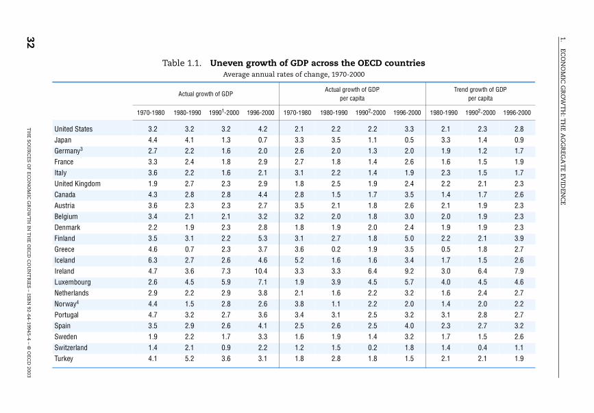
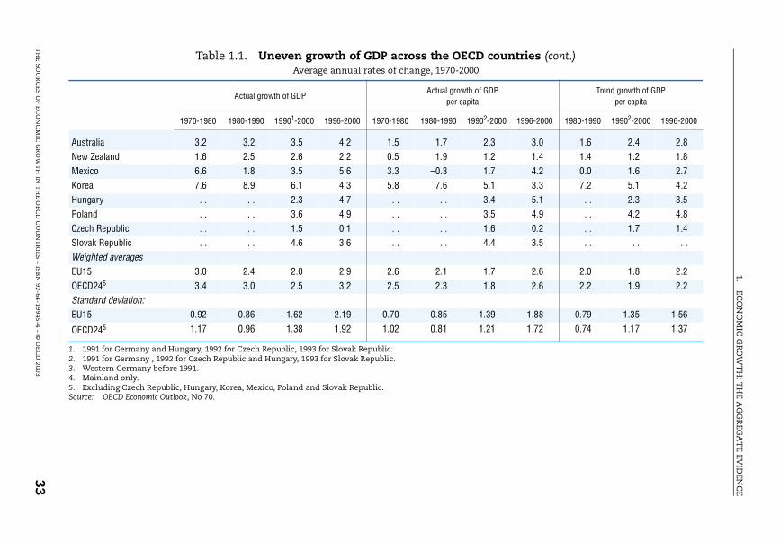
For the OECD area as a whole, cyclically adjusted GDP growth was, onaverage, lower in the 1990s compared with previous decades, continuing thewell-documented long-run slowdown in growth rates (Table 1.1). However, thetrend was reversed in the United States and Canada, as well as in severalsmaller OECD countries (most notably Australia, Ireland, the Netherlands,Norway and Spain). Cyclically adjusted growth rates in GDP per capita – whichare more relevant from a national living standard perspective – presentedbroadly the same picture (Table 1.1).4 These different growth patterns were
associated with a widening of GDP growth disparities in the 1990s whencompared with the 1980s, as shown by the increase in the cross-countrystandard deviation of growth rates.
THE SOURCES OF ECONOMIC GROWTH IN THE OECD COUNTRIES – ISBN 92-64-19945-4 – © OECD 2003 29
1. ECONOMIC GROWTH: THE AGGREGATE EVIDENCE
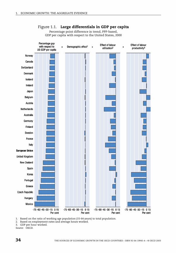
Living standards in 2000: a widening gap across OECD countries
These divergent growth trends over the past decade have also resulted in
widening living-standard conditions in the OECD area. The process ofconvergence that characterised the post-war period and that, albeit at a lowerpace, continued through the 1980s, came to a halt in recent years. Inthe 1990s, there were only a few high-growth countries (e.g. Ireland, Korea)that were still engaged in a process of catch-up, while strong US growth meantthat the gap between its per capita income levels and those of most otherOECD countries started to widen again. Not surprisingly, data for 2000 showthe United States well at the top of the OECD income distribution, followed by
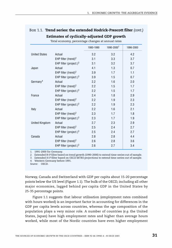
Box 1.1. Trend series: the extended Hodrick-Prescott filter
In this chapter, an attempt is made to identify underlying trends inaggregate variables from observed series. Trend series for output,employment and productivity have been estimated using an extendedversion of the Hodrick-Prescott filter, Hodrick and Prescott, 1997 (seeAnnex 1 for more details). The cyclical component in actual data isseparated from the trend component under the assumption that theformer has only a temporary effect, while the latter persists. The usualproblem of distinguishing between cyclical and trend componentstowards the end of the sample period is tackled in the extended versionof the H-P filter by extending actual data out of the sample usingthe observed average growth rate over the 1990-2000 period. However, if
past growth rates are not reasonable proxies for future growth patterns,this extension may lead to a bias at the end of the filtered series. For themajority of countries, the bias does not appear to be serious: analternative method of extending the data so as to better anchor thesmoothed series – using the projections in the OECD Medium TermReference Scenario,1 (MTRS) – provided broadly similar results. Thereare, however, a few exceptions. Amongst the G-7 countries (see Tablebelow), only in Japan does the use of OECD MTRS projections lead to asomewhat lower cyclically adjusted growth rate over the 1990s. Thesame effect is also present in Ireland, Korea, Mexico and Turkey. Bycontrast, the use of MTRS leads to a higher cyclically adjusted GDPgrowth rate in Greece.
1. In the context of its bi-annual projection exercise, the Economics Department of the OECDproduces a set of medium-term projections, looking out five years. These projectionsassume that at the end of the projection period output will be at its potential andunemployment will reach its structural level. Further details and data can be found atwww.oecd.org/pdf/M00026000/M00026369.pdf. The data used in the table in Box 1.1 are fromEconomic Outlook 70.
30 THE SOURCES OF ECONOMIC GROWTH IN THE OECD COUNTRIES – ISBN 92-64-19945-4 – © OECD 2003
1. ECONOMIC GROWTH: THE AGGREGATE EVIDENCE
Norway, Canada and Switzerland with GDP per capita about 15-20 percentagepoints below the US level (Figure 1.1). The bulk of the OECD, including all othermajor economies, lagged behind per capita GDP in the United States by25-35 percentage points.
Figure 1.1 suggests that labour utilisation (employment rates combinedwith hours worked) is an important factor in accounting for differences in theGDP per capita levels across countries, whereas the age composition of thepopulation plays a very minor role. A number of countries (e.g. the UnitedStates, Japan) have high employment rates and higher than average hoursworked, while most of the Nordic countries have even higher employment
Box 1.1. Trend series: the extended Hodrick-Prescott filter (cont.)
Estimates of cyclically-adjusted GDP growthTotal economy, percentage changes at annual rates
1. 1991-2000 for Germany.2. Extended H-P filter based on trend growth (1990-2000) to extend time-series out of sample.3. Extended H-P filter based on OECD MTRS projections to extend time-series out of sample.4. Western Germany before 1991.Source: OECD.
1980-1990 1990-20001 1996-2000
United States Actual 3.2 3.2 4.2EHP filter (trend)2 3.1 3.3 3.7EHP filter (project.)3 3.1 3.2 3.7
Japan Actual 4.1 1.3 0.7EHP filter (trend)2 3.9 1.7 1.1EHP filter (project.)3 3.9 1.5 0.7
Germany4 Actual 2.2 1.6 2.0EHP filter (trend)2 2.2 1.5 1.7EHP filter (project.)3 2.2 1.5 1.7
France Actual 2.4 1.8 2.9EHP filter (trend)2 2.2 1.9 2.3EHP filter (project.)3 2.2 1.9 2.3
Italy Actual 2.2 1.6 2.1EHP filter (trend)2 2.3 1.7 1.8EHP filter (project.)3 2.3 1.7 1.9
United Kingdom Actual 2.7 2.3 2.9EHP filter (trend)2 2.5 2.4 2.7EHP filter (project.)3 2.5 2.4 2.7
Canada Actual 2.8 2.8 4.4EHP filter (trend)2 2.6 2.8 3.6EHP filter (project.)3 2.6 2.7 3.4
THE SOURCES OF ECONOMIC GROWTH IN THE OECD COUNTRIES – ISBN 92-64-19945-4 – © OECD 2003 31
1.EC
ON
OM
IC G
RO
WT
H: T
HE A
GG
REG
AT
E EVID
ENC
E
32T
HE S
OU
RC
ES O
F EC
ON
OM
IC G
RO
WT
H IN
TH
E OEC
D C
OU
NT
RIES – ISB
N 92-64-19945-4 – ©
OEC
D 2003
ECD countries
f GDP Trend growth of GDPper capita
02-2000 1996-2000 1980-1990 19902-2000 1996-2000
2.2 3.3 2.1 2.3 2.81.1 0.5 3.3 1.4 0.91.3 2.0 1.9 1.2 1.71.4 2.6 1.6 1.5 1.91.4 1.9 2.3 1.5 1.71.9 2.4 2.2 2.1 2.31.7 3.5 1.4 1.7 2.61.8 2.6 2.1 1.9 2.31.8 3.0 2.0 1.9 2.32.0 2.4 1.9 1.9 2.31.8 5.0 2.2 2.1 3.91.9 3.5 0.5 1.8 2.71.6 3.4 1.7 1.5 2.66.4 9.2 3.0 6.4 7.94.5 5.7 4.0 4.5 4.62.2 3.2 1.6 2.4 2.72.2 2.0 1.4 2.0 2.22.5 3.2 3.1 2.8 2.72.5 4.0 2.3 2.7 3.21.4 3.2 1.7 1.5 2.60.2 1.8 1.4 0.4 1.11.8 1.5 2.1 2.1 1.9
Table 1.1. Uneven growth of GDP across the OAverage annual rates of change, 1970-2000
Actual growth of GDPActual growth o
per capita
1970-1980 1980-1990 19901-2000 1996-2000 1970-1980 1980-1990 199
United States 3.2 3.2 3.2 4.2 2.1 2.2Japan 4.4 4.1 1.3 0.7 3.3 3.5Germany3 2.7 2.2 1.6 2.0 2.6 2.0France 3.3 2.4 1.8 2.9 2.7 1.8Italy 3.6 2.2 1.6 2.1 3.1 2.2United Kingdom 1.9 2.7 2.3 2.9 1.8 2.5Canada 4.3 2.8 2.8 4.4 2.8 1.5Austria 3.6 2.3 2.3 2.7 3.5 2.1Belgium 3.4 2.1 2.1 3.2 3.2 2.0Denmark 2.2 1.9 2.3 2.8 1.8 1.9Finland 3.5 3.1 2.2 5.3 3.1 2.7Greece 4.6 0.7 2.3 3.7 3.6 0.2Iceland 6.3 2.7 2.6 4.6 5.2 1.6Ireland 4.7 3.6 7.3 10.4 3.3 3.3Luxembourg 2.6 4.5 5.9 7.1 1.9 3.9Netherlands 2.9 2.2 2.9 3.8 2.1 1.6Norway4 4.4 1.5 2.8 2.6 3.8 1.1Portugal 4.7 3.2 2.7 3.6 3.4 3.1Spain 3.5 2.9 2.6 4.1 2.5 2.6Sweden 1.9 2.2 1.7 3.3 1.6 1.9Switzerland 1.4 2.1 0.9 2.2 1.2 1.5Turkey 4.1 5.2 3.6 3.1 1.8 2.8
1.EC
ON
OM
IC G
RO
WT
H: T
HE A
GG
REG
AT
E EVID
ENC
E
TH
E SOU
RC
ES OF EC
ON
OM
IC G
RO
WT
H IN
TH
E OEC
D C
OU
NT
RIES
– ISB
N 92-64-19945-4 – ©
OE
CD
200333
Table 1.1. Uneven growth of GDP across the OECD countries (cont.)
f GDP Trend growth of GDPper capita
02-2000 1996-2000 1980-1990 19902-2000 1996-2000
2.3 3.0 1.6 2.4 2.81.2 1.4 1.4 1.2 1.81.7 4.2 0.0 1.6 2.75.1 3.3 7.2 5.1 4.23.4 5.1 . . 2.3 3.53.5 4.9 . . 4.2 4.81.6 0.2 . . 1.7 1.44.4 3.5 . . . . . .
1.7 2.6 2.0 1.8 2.21.8 2.6 2.2 1.9 2.2
1.39 1.88 0.79 1.35 1.561.21 1.72 0.74 1.17 1.37
Average annual rates of change, 1970-2000
1. 1991 for Germany and Hungary, 1992 for Czech Republic, 1993 for Slovak Republic.2. 1991 for Germany , 1992 for Czech Republic and Hungary, 1993 for Slovak Republic.3. Western Germany before 1991.4. Mainland only.5. Excluding Czech Republic, Hungary, Korea, Mexico, Poland and Slovak Republic.Source: OECD Economic Outlook, No 70.
Actual growth of GDPActual growth o
per capita
1970-1980 1980-1990 19901-2000 1996-2000 1970-1980 1980-1990 199
Australia 3.2 3.2 3.5 4.2 1.5 1.7New Zealand 1.6 2.5 2.6 2.2 0.5 1.9Mexico 6.6 1.8 3.5 5.6 3.3 –0.3Korea 7.6 8.9 6.1 4.3 5.8 7.6Hungary . . . . 2.3 4.7 . . . .Poland . . . . 3.6 4.9 . . . .Czech Republic . . . . 1.5 0.1 . . . .Slovak Republic . . . . 4.6 3.6 . . . .Weighted averagesEU15 3.0 2.4 2.0 2.9 2.6 2.1OECD245 3.4 3.0 2.5 3.2 2.5 2.3Standard deviation:EU15 0.92 0.86 1.62 2.19 0.70 0.85
OECD245 1.17 0.96 1.38 1.92 1.02 0.81
1. ECONOMIC GROWTH: THE AGGREGATE EVIDENCE
Figure 1.1. Large differentials in GDP per capitaPercentage point difference in trend, PPP-based,
GDP per capita with respect to the United States, 2000
1. Based on the ratio of working age population (15-64 years) to total population.2. Based on employment rates and average hours worked.3. GDP per hour worked.Source: OECD.
-75 -60 -45 -30 -15 0 15 -75 -60 -45 -30 -15 0 15 -75 -60 -45 -30 -15 0 15 -75 -60 -45 -30 -15 0 15
Percentage gapwith respect to
US GDP per capitaDemographic effect1
Per cent Per cent Per cent Per cent
= + +Effect of labour
utilisation2Effect of labourproductivity3
Norway
Canada
Switzerland
Denmark
Iceland
Ireland
Japan
Belgium
Austria
Netherlands
Australia
Germany
Finland
Sweden
France
Italy
European Union
United Kingdom
New Zealand
Spain
Korea
Portugal
Greece
Czech Republic
Hungary
Mexico
34 THE SOURCES OF ECONOMIC GROWTH IN THE OECD COUNTRIES – ISBN 92-64-19945-4 – © OECD 2003
1. ECONOMIC GROWTH: THE AGGREGATE EVIDENCE
rates, but this is offset by lower hours worked. By contrast, low employment
rates in some countries (e.g. Belgium, Netherlands, France, Italy and Spain),combined with relatively low hours, explain more than 20 percentage pointsof the gap between their per capita income and that of the United States.
The contributions of labour productivity and labour utilisation to GDP percapita are interrelated: non-employed people of working age generally havelower education levels – and thus lower potential productivity – than those in
employment. Convergence towards the US level of labour utilisation might,therefore, be associated with a drop in relative productivity in countries withlow labour utilisation. Nevertheless, even if labour productivity at the marginwere only half the average productivity level – a fairly conservativeassumption –, rising labour utilisation in these countries would stillsubstantially raise GDP per capita.
What drove GDP per capita growth in the 1990s?
A useful way of viewing growth in GDP per capita over the past decade isto break it down into three major components, comprising growth rates of:i) the ratio of persons of working-age (15-64 years) to the total population;ii) the ratio of employed persons to the working age population (the“employment rate”); and iii) labour productivity (Figure 1.2).
For the vast majority of OECD countries, demographic trends were arelatively minor component of growth in GDP per capita over the 1990s. Theonly countries where demographic change made a positive and significantcontribution to growth in GDP per capita were Mexico, Korea, Turkey andIreland, the latter having experienced a reversal in traditional migration flowsin the 1990s (OECD, 1999c). However, in some OECD countries, demographictrends have begun (in this accounting sense) to act as a slight drag on growthin GDP per capita. This tendency is set to strengthen in the future due to morerapid increase in the share of older persons in total population (OECD, 1998).
Rising labour productivity, defined as GDP per person employed,accounted for at least half of GDP per capita growth in most OECD countriesover the 1990s. Since hours worked fell in most countries over the 1990s,especially in continental Europe, labour productivity growth was higher on anhourly basis than when measured on a head-count basis. Declines in hoursworked reflect both shorter statutory (or collectively agreed) working weeks aswell as, especially in a number of European countries, a substantial increase inpart-time work.5
Compared with the previous decade, hourly labour productivity pickedup in a number of countries, including the United States, Australia, Norway,Portugal, Germany, Finland and Sweden, while it declined in the othercountries. However, these changes in productivity trend were accompanied by
THE SOURCES OF ECONOMIC GROWTH IN THE OECD COUNTRIES – ISBN 92-64-19945-4 – © OECD 2003 35
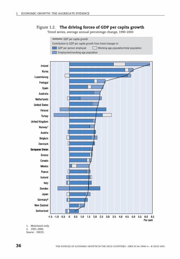
1. ECONOMIC GROWTH: THE AGGREGATE EVIDENCE
Figure 1.2. The driving forces of GDP per capita growthTrend series, average annual percentage change, 1990-2000
1. Mainland only.2. 1991-2000.Source: OECD.
-1.5 -1.0 -0.5 0 0.5 1.0 1.5 2.0 2.5 3.0 3.5 4.0 4.5 5.0 5.5 6.0 6.5
GDP per capita growth
Per cent
Contribution to GDP per capita growth from trend changes in:
GDP per person employed
Employment/working-age population
Working-age population/total population
Ireland
Korea
Luxembourg
Portugal
Spain
Australia
Netherlands
United States
Finland
Turkey
United Kingdom
Norway1
Austria
Belgium
Denmark
European Union
Greece
Canada
Mexico
France
Iceland
Italy
Sweden
Japan
Germany2
New Zealand
Switzerland
36 THE SOURCES OF ECONOMIC GROWTH IN THE OECD COUNTRIES – ISBN 92-64-19945-4 – © OECD 2003

1. ECONOMIC GROWTH: THE AGGREGATE EVIDENCE
different employment patterns across countries. Amongst the G-7 economies,
significant employment increases in the United States (as well as in Canadaand Japan with no acceleration in productivity) contrasted sharply withdeclines in Germany and Italy. Even stronger contrasts in employmentpatterns were found amongst some smaller countries; strong upward trendsin employment rates in Ireland, the Netherlands and Spain compare withdeclines in Finland and Sweden and Turkey.6
1.2. The role of skills and labour utilisation in labour productivity growth
Growth in output per employed person is partly attributable to increasesin the average level of skills, or “human capital”, of those in employment. Thisis illustrated in Figure 1.3, which displays the impact of changes in the averagehuman capital of workers on growth in cyclically adjusted GDP per hourworked. The human-capital adjustment is based on a measure of labour inputthat sums up shares of workers with different levels of formal education, eachweighted by their relative wage. The rationale behind this measure is first that
educational attainment accounts for a good proportion of human capitalembodied in workers; and second, that relative wages between different levelsof education provide a reasonable quantitative proxy for the relativeproductivity of workers with different levels of education (see Box 1.2).7
OECD countries have invested heavily on education over past decadesand this, at least from a pure accounting perspective, resulted in a positive
contribution of human capital enhancement in growth rates of GDP perperson employed.8 Over the past decade, skill upgrading amongst workerswas particularly marked in Europe, where it was accompanied by sluggishemployment growth, productivity gains having been achieved in part bydismissals or not employing workers with low skills.9 By contrast, in theUnited States, Australia, Canada, the Netherlands and New Zealand, skillupgrading has played, at best, a modest role in GDP growth per employedperson: improving labour-market conditions in these countries has widenedthe employment base, especially in the 1990s, allowing low-skilled workers toget a foothold in employment.10
In order to shed further light on this, Figure 1.4 plots changes in the shareof persons in employment with upper-secondary education or above againstchanges in their share in the total working-age population. Up-skilling amongthe employed is largely associated with a generalised improvement in theeducational level of the working-age population (i.e. countries lie close to thediagonal in Figure 1.4). Nevertheless, there has been a tendency foremployment gains to be biased towards the better educated in a number of
European countries (i.e. they are located above the diagonal). By contrast,
THE SOURCES OF ECONOMIC GROWTH IN THE OECD COUNTRIES – ISBN 92-64-19945-4 – © OECD 2003 37
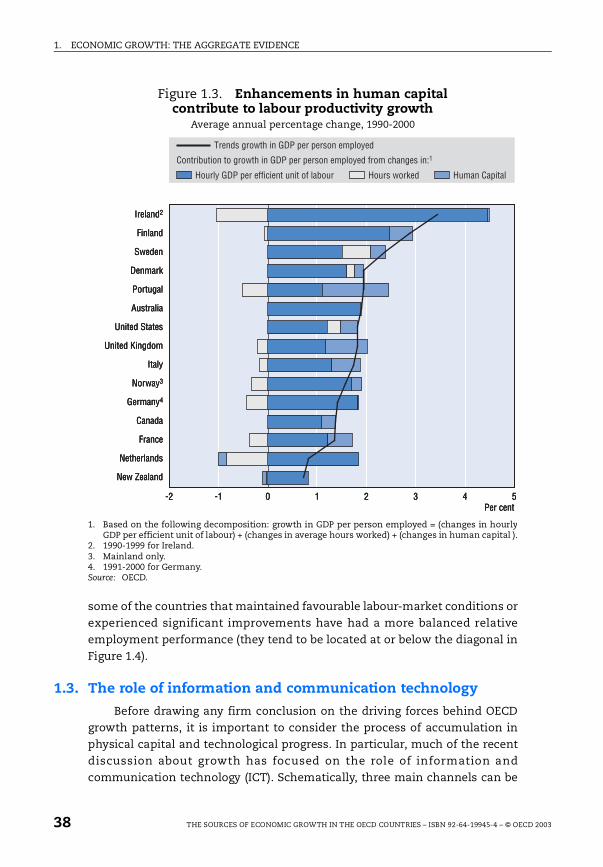
1. ECONOMIC GROWTH: THE AGGREGATE EVIDENCE
some of the countries that maintained favourable labour-market conditions orexperienced significant improvements have had a more balanced relativeemployment performance (they tend to be located at or below the diagonal inFigure 1.4).
1.3. The role of information and communication technology
Before drawing any firm conclusion on the driving forces behind OECDgrowth patterns, it is important to consider the process of accumulation inphysical capital and technological progress. In particular, much of the recentdiscussion about growth has focused on the role of information andcommunication technology (ICT). Schematically, three main channels can be
Figure 1.3. Enhancements in human capital contribute to labour productivity growth
Average annual percentage change, 1990-2000
1. Based on the following decomposition: growth in GDP per person employed = (changes in hourlyGDP per efficient unit of labour) + (changes in average hours worked) + (changes in human capital ).
2. 1990-1999 for Ireland.3. Mainland only.4. 1991-2000 for Germany.Source: OECD.
-2 -1 0 1 2 3 4 5
Trends growth in GDP per person employed
Per cent
Contribution to growth in GDP per person employed from changes in:1
Hourly GDP per efficient unit of labour Human CapitalHours worked
Ireland2
Finland
Sweden
Denmark
Portugal
Australia
United States
United Kingdom
Italy
Norway3
Germany4
Canada
France
Netherlands
New Zealand
38 THE SOURCES OF ECONOMIC GROWTH IN THE OECD COUNTRIES – ISBN 92-64-19945-4 – © OECD 2003
1. ECONOMIC GROWTH: THE AGGREGATE EVIDENCE
identified through which ICT can affect potential growth rates: i) anacceleration of productivity in the ICT-producing sectors themselves, and a
growing size of ICT-producing sectors in the economy; ii) capital deepeningacross the economy, driven by rapid investment in ICT equipment, andresulting in a boost to labour productivity; and iii) widespread spillover effectson productivity arising from IC technology. This section focuses on the firsttwo contributions of ICT, while the third is discussed in the next section in thebroader context of the analysis of MFP trends.
The ICT-producing sector
Figure 1.5 shows the share of the ICT sector in total value-added of thebusiness sector in a group of OECD countries.11 In 1999, the ICT sector
Box 1.2. Estimating changes in the quality of factor inputs: the example of the labour input
In order to assess the impact of the labour and capital inputs in outputand productivity growth rates, proper account should be taken of therole that each factor plays as input in the production process. In the caseof labour input, the simple count of hours worked is only a crudeapproximation, insofar as workers show great differences in education,experience, sector of activity and other attributes which greatly affect
their marginal productivity. In particular, a measure of labour input inefficiency units can be obtained by weighting different types of labour bytheir marginal contribution to the production activity in which they areemployed. Since these productivity measures are generally notobservable, information on relative wages by characteristics is used toderive the required weights to aggregate different types of labour. Thedifference between the weighted and un-weighted series yields an indexfor the compositional change of labour input, or its quality.
To take into account the effect of changes in the composition of labourinput, six different types of workers were considered, based on genderand three different educational levels: below upper-secondary; upper-secondary and tertiary education. It is assumed that: i) workers withdifferent levels of education work the same (average) number of hours;and ii) relative wage rates are constant over the sample period.Compared with other proxies available in the literature (largely for theUnited States) this decomposition is rather crude, but it does shed lighton the role of compositional changes in labour input consistently for arange of OECD countries, thereby permitting cross-country comparisons.
For more details on this procedure, see Annex 1.
THE SOURCES OF ECONOMIC GROWTH IN THE OECD COUNTRIES – ISBN 92-64-19945-4 – © OECD 2003 39
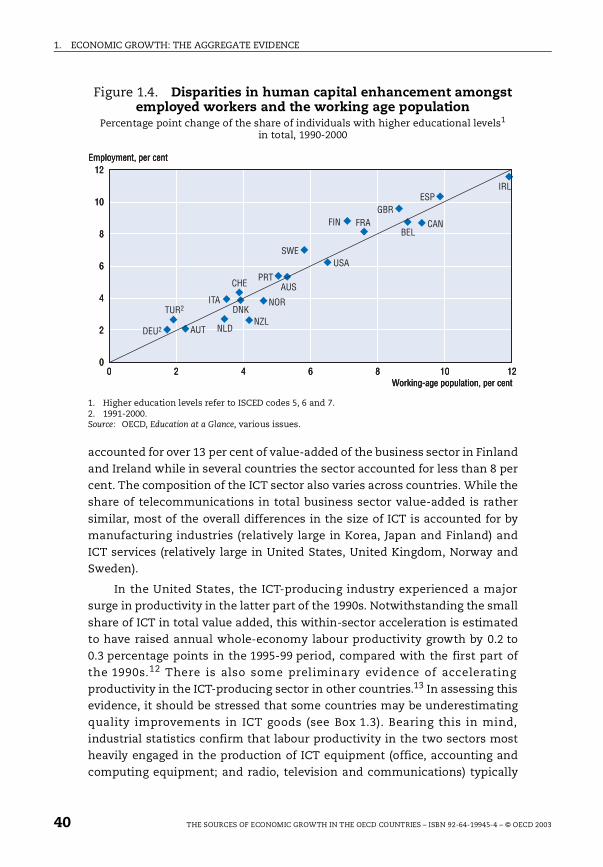
1. ECONOMIC GROWTH: THE AGGREGATE EVIDENCE
accounted for over 13 per cent of value-added of the business sector in Finlandand Ireland while in several countries the sector accounted for less than 8 percent. The composition of the ICT sector also varies across countries. While theshare of telecommunications in total business sector value-added is rather
similar, most of the overall differences in the size of ICT is accounted for bymanufacturing industries (relatively large in Korea, Japan and Finland) andICT services (relatively large in United States, United Kingdom, Norway andSweden).
In the United States, the ICT-producing industry experienced a majorsurge in productivity in the latter part of the 1990s. Notwithstanding the small
share of ICT in total value added, this within-sector acceleration is estimatedto have raised annual whole-economy labour productivity growth by 0.2 to0.3 percentage points in the 1995-99 period, compared with the first part ofthe 1990s.12 There is also some preliminary evidence of acceleratingproductivity in the ICT-producing sector in other countries.13 In assessing thisevidence, it should be stressed that some countries may be underestimatingquality improvements in ICT goods (see Box 1.3). Bearing this in mind,industrial statistics confirm that labour productivity in the two sectors mostheavily engaged in the production of ICT equipment (office, accounting andcomputing equipment; and radio, television and communications) typically
Figure 1.4. Disparities in human capital enhancement amongst employed workers and the working age population
Percentage point change of the share of individuals with higher educational levels1 in total, 1990-2000
1. Higher education levels refer to ISCED codes 5, 6 and 7.2. 1991-2000.Source: OECD, Education at a Glance, various issues.
0 2 4 6 8 10 12
12
10
8
6
4
2
0
DEU2
TUR2
AUT NLD
CHE
ITADNK
NZL
NOR
PRTAUS
SWEUSA
FIN FRAGBR
BELCAN
ESPIRL
Employment, per cent
Working-age population, per cent0 2 4 6 8 10 12
12
10
8
6
4
2
0
DEU2
TUR2
AUT NLD
CHE
ITADNK
NZL
NOR
PRTAUS
SWEUSA
FIN FRAGBR
BELCAN
ESPIRL
Employment, per cent
Working-age population, per cent0 2 4 6 8 10 12
12
10
8
6
4
2
0
DEU2
TUR2
AUT NLD
CHE
ITADNK
NZL
NOR
PRTAUS
SWEUSA
FIN FRAGBR
BELCAN
ESPIRL
Employment, per cent
Working-age population, per cent
40 THE SOURCES OF ECONOMIC GROWTH IN THE OECD COUNTRIES – ISBN 92-64-19945-4 – © OECD 2003
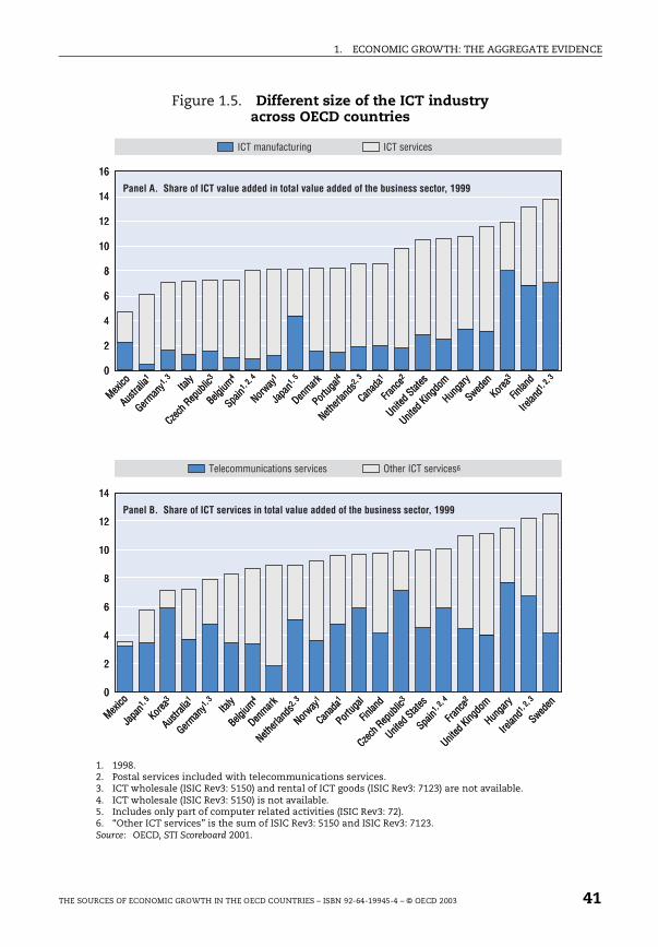
1. ECONOMIC GROWTH: THE AGGREGATE EVIDENCE
Figure 1.5. Different size of the ICT industry across OECD countries
1. 1998.2. Postal services included with telecommunications services.3. ICT wholesale (ISIC Rev3: 5150) and rental of ICT goods (ISIC Rev3: 7123) are not available.4. ICT wholesale (ISIC Rev3: 5150) is not available.5. Includes only part of computer related activities (ISIC Rev3: 72).6. “Other ICT services” is the sum of ISIC Rev3: 5150 and ISIC Rev3: 7123.Source: OECD, STI Scoreboard 2001.
16
14
12
10
8
6
4
2
0
14
12
10
8
6
4
2
0
ICT manufacturing ICT services
Mexico
Austra
lia1
Mexico
Japa
n1, 5
Korea3
Austra
lia1
German
y1, 3
Italy
Belgium
4
Denmark
Netherl
ands
2, 3
Norway
1
Canad
a1
Portug
al
Finlan
d
Czech R
epub
lic3
United
States
Spain1,
2, 4
Franc
e2
United
Kingdo
m
Hunga
ry
Irelan
d1, 2
, 3
Sweden
German
y1, 3
Italy
Czech R
epub
lic3
Belgium
4
Spain1,
2, 4
Norway
1
Japa
n1, 5
Denmark
Portug
al4
Netherl
ands
2, 3
Canad
a1
Franc
e2
United
States
United
Kingdo
m
Hunga
ry
Sweden
Korea3
Finlan
d
Irelan
d1, 2
, 3
Panel A. Share of ICT value added in total value added of the business sector, 1999
Telecommunications services Other ICT services6
Panel B. Share of ICT services in total value added of the business sector, 1999
THE SOURCES OF ECONOMIC GROWTH IN THE OECD COUNTRIES – ISBN 92-64-19945-4 – © OECD 2003 41
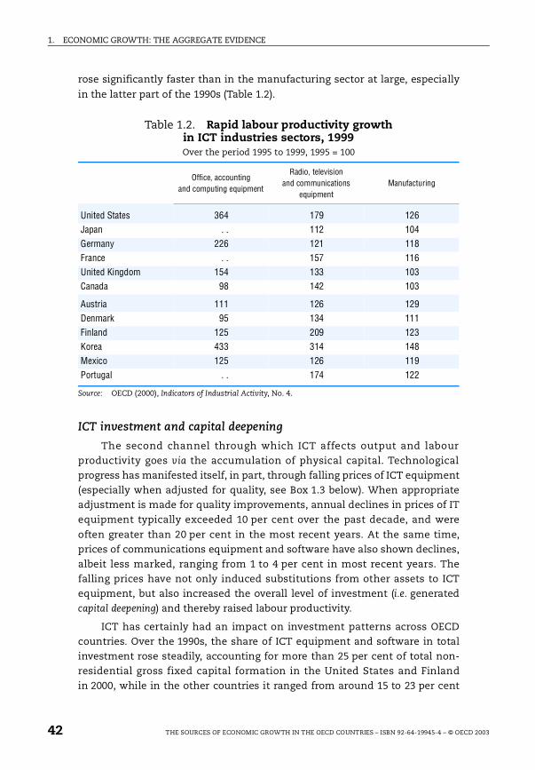
1. ECONOMIC GROWTH: THE AGGREGATE EVIDENCE
rose significantly faster than in the manufacturing sector at large, especially
in the latter part of the 1990s (Table 1.2).
ICT investment and capital deepening
The second channel through which ICT affects output and labourproductivity goes via the accumulation of physical capital. Technologicalprogress has manifested itself, in part, through falling prices of ICT equipment(especially when adjusted for quality, see Box 1.3 below). When appropriateadjustment is made for quality improvements, annual declines in prices of ITequipment typically exceeded 10 per cent over the past decade, and were
often greater than 20 per cent in the most recent years. At the same time,prices of communications equipment and software have also shown declines,albeit less marked, ranging from 1 to 4 per cent in most recent years. Thefalling prices have not only induced substitutions from other assets to ICTequipment, but also increased the overall level of investment (i.e. generatedcapital deepening) and thereby raised labour productivity.
ICT has certainly had an impact on investment patterns across OECDcountries. Over the 1990s, the share of ICT equipment and software in totalinvestment rose steadily, accounting for more than 25 per cent of total non-residential gross fixed capital formation in the United States and Finlandin 2000, while in the other countries it ranged from around 15 to 23 per cent
Table 1.2. Rapid labour productivity growth in ICT industries sectors, 1999Over the period 1995 to 1999, 1995 = 100
Source: OECD (2000), Indicators of Industrial Activity, No. 4.
Office, accounting and computing equipment
Radio, television and communications
equipmentManufacturing
United States 364 179 126Japan . . 112 104Germany 226 121 118France . . 157 116United Kingdom 154 133 103Canada 98 142 103
Austria 111 126 129Denmark 95 134 111Finland 125 209 123Korea 433 314 148Mexico 125 126 119Portugal . . 174 122
42 THE SOURCES OF ECONOMIC GROWTH IN THE OECD COUNTRIES – ISBN 92-64-19945-4 – © OECD 2003
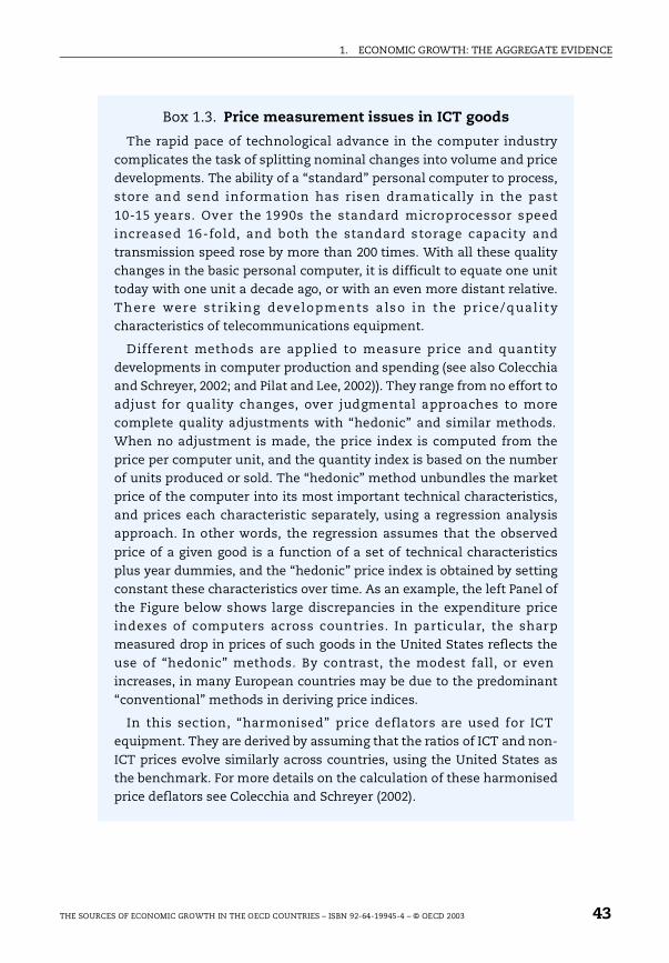
1. ECONOMIC GROWTH: THE AGGREGATE EVIDENCE
Box 1.3. Price measurement issues in ICT goods
The rapid pace of technological advance in the computer industrycomplicates the task of splitting nominal changes into volume and pricedevelopments. The ability of a “standard” personal computer to process,store and send information has risen dramatically in the past
10-15 years. Over the 1990s the standard microprocessor speedincreased 16-fold, and both the standard storage capacity andtransmission speed rose by more than 200 times. With all these qualitychanges in the basic personal computer, it is difficult to equate one unittoday with one unit a decade ago, or with an even more distant relative.There were str ik ing developments a lso in the price/qualitycharacteristics of telecommunications equipment.
Different methods are applied to measure price and quantitydevelopments in computer production and spending (see also Colecchiaand Schreyer, 2002; and Pilat and Lee, 2002)). They range from no effort toadjust for quality changes, over judgmental approaches to morecomplete quality adjustments with “hedonic” and similar methods.When no adjustment is made, the price index is computed from theprice per computer unit, and the quantity index is based on the numberof units produced or sold. The “hedonic” method unbundles the marketprice of the computer into its most important technical characteristics,and prices each characteristic separately, using a regression analysisapproach. In other words, the regression assumes that the observed
price of a given good is a function of a set of technical characteristicsplus year dummies, and the “hedonic” price index is obtained by settingconstant these characteristics over time. As an example, the left Panel ofthe Figure below shows large discrepancies in the expenditure priceindexes of computers across countries. In particular, the sharpmeasured drop in prices of such goods in the United States reflects theuse of “hedonic” methods. By contrast, the modest fall, or evenincreases, in many European countries may be due to the predominant“conventional” methods in deriving price indices.
In this section, “harmonised” price deflators are used for ICTequipment. They are derived by assuming that the ratios of ICT and non-ICT prices evolve similarly across countries, using the United States asthe benchmark. For more details on the calculation of these harmonisedprice deflators see Colecchia and Schreyer (2002).
THE SOURCES OF ECONOMIC GROWTH IN THE OECD COUNTRIES – ISBN 92-64-19945-4 – © OECD 2003 43
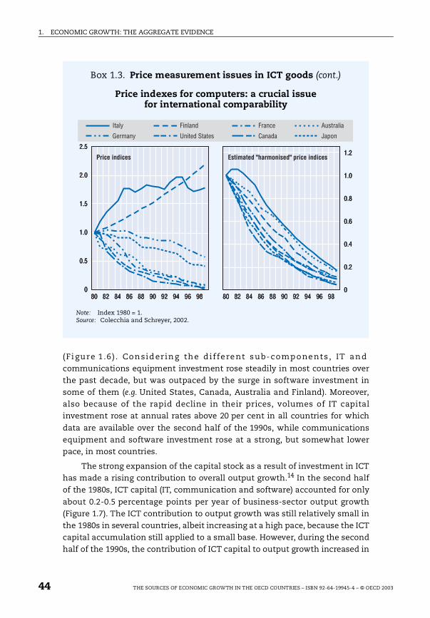
1. ECONOMIC GROWTH: THE AGGREGATE EVIDENCE
(Fi gure 1 .6 ) . Consid ering the d ifferent sub-comp onents , IT andcommunications equipment investment rose steadily in most countries overthe past decade, but was outpaced by the surge in software investment insome of them (e.g. United States, Canada, Australia and Finland). Moreover,also because of the rapid decline in their prices, volumes of IT capitalinvestment rose at annual rates above 20 per cent in all countries for which
data are available over the second half of the 1990s, while communicationsequipment and software investment rose at a strong, but somewhat lowerpace, in most countries.
The strong expansion of the capital stock as a result of investment in ICThas made a rising contribution to overall output growth.14 In the second halfof the 1980s, ICT capital (IT, communication and software) accounted for only
about 0.2-0.5 percentage points per year of business-sector output growth(Figure 1.7). The ICT contribution to output growth was still relatively small inthe 1980s in several countries, albeit increasing at a high pace, because the ICTcapital accumulation still applied to a small base. However, during the secondhalf of the 1990s, the contribution of ICT capital to output growth increased in
Box 1.3. Price measurement issues in ICT goods (cont.)
Price indexes for computers: a crucial issue for international comparability
Note: Index 1980 = 1.Source: Colecchia and Schreyer, 2002.
80 82 84 86 88 90 92 94 96 98
2.5
2.0
1.5
1.0
0.5
080 82 84 86 88 90 92 94 96 98
1.2
1.0
0.8
0.6
0.4
0.2
0
Italy Finland France Australia
Germany United States Canada Japon
Price indices Estimated "harmonised" price indices
80 82 84 86 88 90 92 94 96 98
2.5
2.0
1.5
1.0
0.5
080 82 84 86 88 90 92 94 96 98
1.2
1.0
0.8
0.6
0.4
0.2
0
Italy Finland France Australia
Germany United States Canada Japon
Price indices Estimated "harmonised" price indices
80 82 84 86 88 90 92 94 96 98
2.5
2.0
1.5
1.0
0.5
080 82 84 86 88 90 92 94 96 98
1.2
1.0
0.8
0.6
0.4
0.2
0
Italy Finland France Australia
Germany United States Canada Japon
Price indices Estimated "harmonised" price indices
44 THE SOURCES OF ECONOMIC GROWTH IN THE OECD COUNTRIES – ISBN 92-64-19945-4 – © OECD 2003
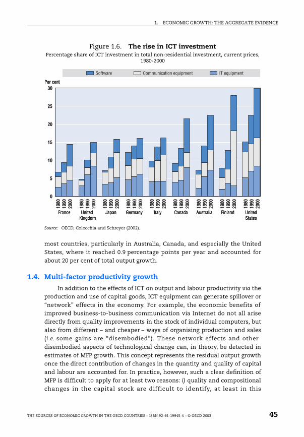
1. ECONOMIC GROWTH: THE AGGREGATE EVIDENCE
most countries, particularly in Australia, Canada, and especially the UnitedStates, where it reached 0.9 percentage points per year and accounted forabout 20 per cent of total output growth.
1.4. Multi-factor productivity growth
In addition to the effects of ICT on output and labour productivity via theproduction and use of capital goods, ICT equipment can generate spillover or“network” effects in the economy. For example, the economic benefits ofimproved business-to-business communication via Internet do not all arisedirectly from quality improvements in the stock of individual computers, butalso from different – and cheaper – ways of organising production and sales(i.e. some gains are “disembodied”). These network effects and other
disembodied aspects of technological change can, in theory, be detected inestimates of MFP growth. This concept represents the residual output growthonce the direct contribution of changes in the quantity and quality of capitaland labour are accounted for. In practice, however, such a clear definition ofMFP is difficult to apply for at least two reasons: i) quality and compositionalchanges in the capital stock are difficult to identify, at least in this
Figure 1.6. The rise in ICT investmentPercentage share of ICT investment in total non-residential investment, current prices,
1980-2000
Source: OECD, Colecchia and Schreyer (2002).
30
25
20
15
10
5
0
1980
1990
2000
1980
1990
2000
1980
1990
2000
1980
1990
2000
1980
1990
2000
1980
1990
2000
1980
1990
2000
1980
1990
2000
1980
1990
2000
Software IT equipmentCommunication equipment
Per cent
France United Kingdom
Japan Germany Italy Canada Australia Finland UnitedStates
30
25
20
15
10
5
0
1980
1990
2000
1980
1990
2000
1980
1990
2000
1980
1990
2000
1980
1990
2000
1980
1990
2000
1980
1990
2000
1980
1990
2000
1980
1990
2000
Software IT equipmentCommunication equipment
Per cent
France United Kingdom
Japan Germany Italy Canada Australia Finland UnitedStates
30
25
20
15
10
5
0
1980
1990
2000
1980
1990
2000
1980
1990
2000
1980
1990
2000
1980
1990
2000
1980
1990
2000
1980
1990
2000
1980
1990
2000
1980
1990
2000
Software IT equipmentCommunication equipment
Per cent
France United Kingdom
Japan Germany Italy Canada Australia Finland UnitedStates
THE SOURCES OF ECONOMIC GROWTH IN THE OECD COUNTRIES – ISBN 92-64-19945-4 – © OECD 2003 45
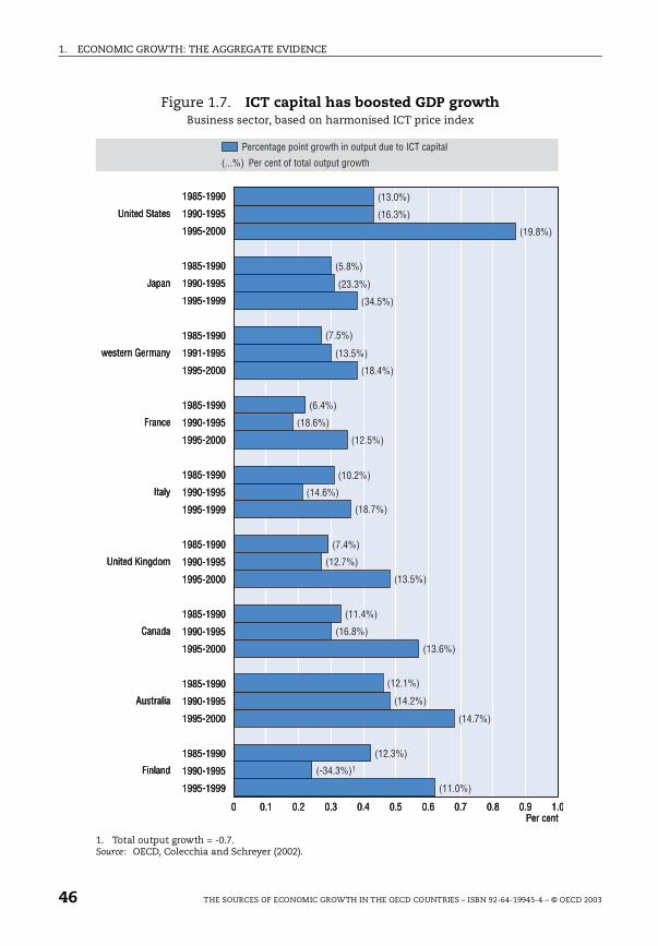
1. ECONOMIC GROWTH: THE AGGREGATE EVIDENCE
Figure 1.7. ICT capital has boosted GDP growthBusiness sector, based on harmonised ICT price index
1. Total output growth = -0.7.Source: OECD, Colecchia and Schreyer (2002).
1985-1990
1990-1995
1995-2000
1985-1990
1990-1995
1995-1999
1985-1990
1991-1995
1995-2000
1985-1990
1990-1995
1995-2000
1985-1990
1990-1995
1995-1999
1985-1990
1990-1995
1995-2000
1985-1990
1990-1995
1995-2000
1985-1990
1990-1995
1995-2000
1985-1990
1990-1995
1995-1999
0 0.1 0.2 0.3 0.4 0.5 0.6 0.7 0.8 0.9 1.0
(13.0%)
(16.3%)
(5.8%)
(23.3%)
(7.5%)
(13.5%)
(18.4%)
(6.4%)
(18.6%)
(12.5%)
(10.2%)
(14.6%)
(18.7%)
(7.4%)
(12.7%)
(13.5%)
(11.4%)
(16.8%)
(13.6%)
(12.1%)
(14.2%)
(14.7%)
(12.3%)
(-34.3%)1
(11.0%)
(34.5%)
(19.8%)
Percentage point growth in output due to ICT capital
(...%) Per cent of total output growth
Per cent
United States
Japan
western Germany
France
Italy
United Kingdom
Canada
Australia
Finland
1985-1990
1990-1995
1995-2000
1985-1990
1990-1995
1995-1999
1985-1990
1991-1995
1995-2000
1985-1990
1990-1995
1995-2000
1985-1990
1990-1995
1995-1999
1985-1990
1990-1995
1995-2000
1985-1990
1990-1995
1995-2000
1985-1990
1990-1995
1995-2000
1985-1990
1990-1995
1995-1999
0 0.1 0.2 0.3 0.4 0.5 0.6 0.7 0.8 0.9 1.0
(13.0%)
(16.3%)
(5.8%)
(23.3%)
(7.5%)
(13.5%)
(18.4%)
(6.4%)
(18.6%)
(12.5%)
(10.2%)
(14.6%)
(18.7%)
(7.4%)
(12.7%)
(13.5%)
(11.4%)
(16.8%)
(13.6%)
(12.1%)
(14.2%)
(14.7%)
(12.3%)
(-34.3%)1
(11.0%)
(34.5%)
(19.8%)
Percentage point growth in output due to ICT capital
(...%) Per cent of total output growth
Per cent
United States
Japan
western Germany
France
Italy
United Kingdom
Canada
Australia
Finland
46 THE SOURCES OF ECONOMIC GROWTH IN THE OECD COUNTRIES – ISBN 92-64-19945-4 – © OECD 2003
1. ECONOMIC GROWTH: THE AGGREGATE EVIDENCE
international comparison (see Box 1.4), and are partially left in the
productivity residual; and ii) for a number of countries, available data do notallow the assessment of the direct or indirect effects of ICT (nor othercompositional/quality changes in capital) but, again, these are captured by theproductivity residual.
Following these arguments, Table 1.3 presents different measures ofcyclically adjusted MFP growth rates in the business sector of nine countries
over the past decades.15 The first measure is computed considering aggregatehours worked and gross capital stock as inputs (i.e. not adjusted for changes inthe quality of labour and capital inputs). This is the broadest measure ofproductivity growth that incorporates the effects of progress in human capitalas well as embodied (in physical capital) and disembodied technologicalprogress. The second measure corrects for the general rise in education levelsby using a quality-adjusted measure of labour input. Finally, the third measureof the residual also takes into account changes in the “quality” andcomposition of the capital stock input (see Box 1.4). This measure can beconsidered as a proxy for the truly disembodied technological progress,although the decomposition of capital assets is still very limited and,therefore, does not capture shifts occurring at a finer level of disaggregation.
For other OECD countries, only the first measures of MFP could be calculated(see Figure 1.8).
Comparisons of the different MFP estimates in Table 1.3 indicatesignificant variation amongst the G-7 countries, Australia and Finland. TheUnited States, Canada and Australia recorded a recovery in MFP growth in
the 1990s that reversed a longstanding downward trend. Conversely, allmeasures of MFP growth rates decreased significantly in Germany, France andItaly.
The correction for changes in the composition of labour and capitalinputs tends to reduce measured MFP, insofar as part of the output growth isassigned to improvements in the quality of factors used in the production
process (i.e. embodied in inputs) rather than to changes in productivity. In theUnited States, contributions of human capital and quality-driven ICT-capitaldeepening were limited to about 0.2 percentage points in the early 1980s.However, while the role of human capital enhancement is unchanged, thecontribution of ICT to embodied technological progress (reflecting thedifference between the growth rate of quality-adjusted MFP and the othermeasures) has increased over time to peak in the second half of the 1990s, asa result of a faster pace of ICT adoption. Hence, the spread of ICT in the UnitedStates seems to have first emerged as disembodied MFP growth (probably inthe ICT-producing sector) but, more recently, it has also emerged intechnological progress embodied in new ICT equipment used in many sectors(see also Oliner and Sichel, 2001). Similar patterns are also observed in Finland
THE SOURCES OF ECONOMIC GROWTH IN THE OECD COUNTRIES – ISBN 92-64-19945-4 – © OECD 2003 47

1. ECONOMIC GROWTH: THE AGGREGATE EVIDENCE
Box 1.4. Measures of multi-factor productivity (MFP)
Estimates of multi-factor productivity (MFP) growth are often used toproxy technological progress. They are obtained as the residual outputgrowth once the weighted contributions of changes in capital and labourinputs are accounted for. Therefore, MFP growth estimates involve a
number of assumptions concerning the measurement of output andinput. In the case of labour, changes in skills and educational attainmentneed to be explicitly taken into account (see above). In the case of capital,quantities and prices should be adjusted for changes in quality.Moreover, measures of growth rates of MFP can be sensitive toaggregation methods. This may be the case particularly when quantitiesand user costs of some disaggregated inputs evolve along differentpatterns than those of the corresponding aggregate input. This is thecase, for example, when quality improvements in some particularcapital inputs (such as ICT) are faster than those in others.
A measure of MFP growth that fully accounts for changes in thecomposition and quality of both labour and capital inputs capturesdisembodied technological and organisational improvements thatincrease output for a given amount of inputs. However, it may also beinteresting to assess the extent to which improvements in the quality ofcapital and labour have boosted productivity in industries and countriesthat have invested in them. For example, the shift towards ICT assets,whose relative prices have been falling, implies that with the same
amount of resources it is possible to acquire a greater amount ofproductive capital services. This suggests that there is also an“embodied” element of technological change due to the expansion of theproductive capacity from the shift toward ICT assets (see Greenwoodet al. 1997, Hercowitz, 1998 for a discussion of this issue).1
The weighting of factor inputs in the calculation of the MFP growth
residual also involves some measurement problems. In theory it shouldcorrespond to the marginal productivity of labour and capital. Howeverthe latter are not directly observable and a standard choice in theliterature is to assume them to be equal to income shares, given that thelabour share can be easily computed from national accounts. Thiscorresponds to making a few assumptions, most importantly that theproduct and input markets are perfectly competitive and that there areconstant returns to scale (Morrison, 1999). Furthermore, it is oftenassumed that elasticities are constant across the whole period ofobservation (implicitly making the assumption of unit elasticity of
48 THE SOURCES OF ECONOMIC GROWTH IN THE OECD COUNTRIES – ISBN 92-64-19945-4 – © OECD 2003
1. ECONOMIC GROWTH: THE AGGREGATE EVIDENCE
and Australia, where the boost to productivity from ICT adoption is one of thestrongest amongst the countries reported in the table.
Given data limitations, the comparison of MFP growth rates for a widerset of OECD countries has to rely on the broader measure that incorporateschanges in human and physical capital (Figure 1.7). In addition to thecountries mentioned above, Denmark, Ireland, New Zealand, Norway andSweden experienced an increase in their average growth rates of MFP (in mostcases from relatively low rates in the 1980s).
It should be stressed that the context in which the acceleration in MFPgrowth rates has taken place differs across countries and needs to be clarified.In the case of Australia, Canada, Ireland, New Zealand, Norway and the UnitedStates, the acceleration in MFP growth has gone hand-in-hand with high, andoften rising, labour utilisation and rapid GDP per capita growth. In contrast, inFinland and especially Sweden, increases in MFP growth rates have been
accompanied by a slow-down in GDP per capita growth rates and significantfalls in employment rates. In these latter cases, severe macroeconomic crisesin the early 1990s most likely led to cleansing the least productive activitieswith major employment losses, but also with an increase in the recordedaverage MFP growth. Hence, their pattern of MFP growth not only reflects anacceleration of technical change, but also a one-shot reduction ofinefficiencies.
Finally, available data do not allow a clear identification of spillovereffects (i.e. a boost to disembodied technological progress) in ICT-usingsectors, reflecting measurement difficulties as well as the fact that most
Box 1.4. Measures of multi-factor productivity (MFP) (cont.)
substitution between factors) and equal to the observed average.Alternatively it can be recognised that elasticities can vary significantlyfor reasons other than measurement errors and as a discrete timeapproximation, the simple average of factor shares for each couple of
subsequent years can be used. This is the approach used in this chapter.For a sensitivity analysis of the estimates obtained with this approachand those obtained using elasticities estimated econometrically,see Scarpetta et al. (2000).
1. As suggested by Bassanini et al. (2000), a proxy for total (embodied and disembodied)technological change can be computed as the residual from a growth accounting exercise inwhich the standard measure of capital stock (deflated at real acquisition prices) is used,instead of the measure of capital service that incorporates changes in both quality andcomposition. Quality changes only refer to the ICT assets and are proxied by the differencesin growth rates of hedonic and non-hedonic price indexes of ICT. Composition and qualityeffects are estimated by considering seven types of capital goods (Colecchia and Schreyer,2002). See Annex 1 for more details.
THE SOURCES OF ECONOMIC GROWTH IN THE OECD COUNTRIES – ISBN 92-64-19945-4 – © OECD 2003 49
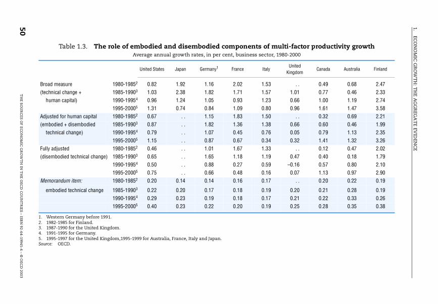
1.EC
ON
OM
IC G
RO
WT
H: T
HE A
GG
REG
AT
E EVID
ENC
E
50T
HE S
OU
RC
ES O
F EC
ON
OM
IC G
RO
WT
H IN
TH
E OEC
D C
OU
NT
RIES – ISB
N 92-64-19945-4 – ©
OEC
D 2003
multi-factor productivity growthor, 1980-2000
yUnited
KingdomCanada Australia Finland
3 . . 0.49 0.68 2.477 1.01 0.77 0.46 2.333 0.66 1.00 1.19 2.740 0.96 1.61 1.47 3.580 . . 0.32 0.69 2.218 0.66 0.60 0.46 1.996 0.05 0.79 1.13 2.354 0.32 1.41 1.32 3.263 . . 0.12 0.47 2.029 0.47 0.40 0.18 1.799 –0.16 0.57 0.80 2.106 0.07 1.13 0.97 2.907 . . 0.20 0.22 0.19
9 0.20 0.21 0.28 0.197 0.21 0.22 0.33 0.269 0.25 0.28 0.35 0.38
Table 1.3. The role of embodied and disembodied components ofAverage annual growth rates, in per cent, business sect
1. Western Germany before 1991.2. 1982-1985 for Finland.3. 1987-1990 for the United Kingdom.4. 1991-1995 for Germany.5. 1995-1997 for the United Kingdom,1995-1999 for Australia, France, Italy and Japan.Source: OECD.
United States Japan Germany1 France Ital
Broad measure 1980-19852 0.82 1.92 1.16 2.02 1.5(technical change + 1985-19903 1.03 2.38 1.82 1.71 1.5
human capital) 1990-19954 0.96 1.24 1.05 0.93 1.21995-20005 1.31 0.74 0.84 1.09 0.8
Adjusted for human capital 1980-19852 0.67 . . 1.15 1.83 1.5(embodied + disembodied 1985-19903 0.87 . . 1.82 1.36 1.3
technical change) 1990-19954 0.79 . . 1.07 0.45 0.71995-20005 1.15 . . 0.87 0.67 0.3
Fully adjusted 1980-19852 0.46 . . 1.01 1.67 1.3(disembodied technical change) 1985-19903 0.65 . . 1.65 1.18 1.1
1990-19954 0.50 . . 0.88 0.27 0.51995-20005 0.75 . . 0.66 0.48 0.1
Memorandum item: 1980-19852 0.20 0.14 0.14 0.16 0.1
embodied technical change 1985-19903 0.22 0.20 0.17 0.18 0.11990-19954 0.29 0.23 0.19 0.18 0.11995-20005 0.40 0.23 0.22 0.20 0.1
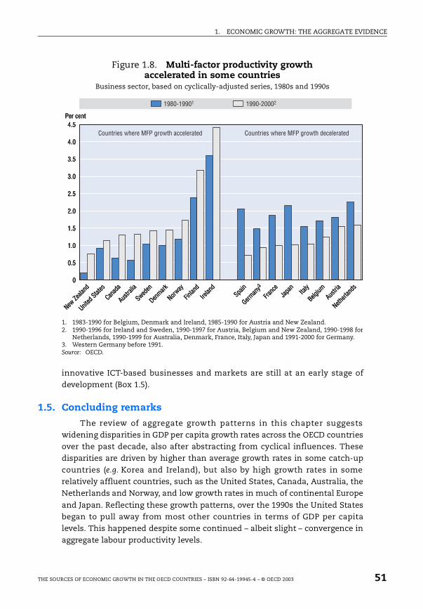
1. ECONOMIC GROWTH: THE AGGREGATE EVIDENCE
innovative ICT-based businesses and markets are still at an early stage ofdevelopment (Box 1.5).
1.5. Concluding remarks
The review of aggregate growth patterns in this chapter suggestswidening disparities in GDP per capita growth rates across the OECD countriesover the past decade, also after abstracting from cyclical influences. Thesedisparities are driven by higher than average growth rates in some catch-upcountries (e.g. Korea and Ireland), but also by high growth rates in somerelatively affluent countries, such as the United States, Canada, Australia, theNetherlands and Norway, and low growth rates in much of continental Europe
and Japan. Reflecting these growth patterns, over the 1990s the United Statesbegan to pull away from most other countries in terms of GDP per capitalevels. This happened despite some continued – albeit slight – convergence inaggregate labour productivity levels.
Figure 1.8. Multi-factor productivity growth accelerated in some countries
Business sector, based on cyclically-adjusted series, 1980s and 1990s
1. 1983-1990 for Belgium, Denmark and Ireland, 1985-1990 for Austria and New Zealand.2. 1990-1996 for Ireland and Sweden, 1990-1997 for Austria, Belgium and New Zealand, 1990-1998 for
Netherlands, 1990-1999 for Australia, Denmark, France, Italy, Japan and 1991-2000 for Germany.3. Western Germany before 1991.Source: OECD.
4.5
4.0
3.5
3.0
2.5
2.0
1.5
1.0
0.5
0
1980-19901 1990-20002
Per cent
Countries where MFP growth accelerated Countries where MFP growth decelerated
New Ze
aland
United
States
Canad
a
Austra
lia
Sweden
Denmark
Norway
Finlan
d
Irelan
dSpa
in
German
y3
Franc
eJa
pan
Italy
Belgium
Austria
Netherl
ands
4.5
4.0
3.5
3.0
2.5
2.0
1.5
1.0
0.5
0
1980-19901 1990-20002
Per cent
Countries where MFP growth accelerated Countries where MFP growth decelerated
New Ze
aland
United
States
Canad
a
Austra
lia
Sweden
Denmark
Norway
Finlan
d
Irelan
dSpa
in
German
y3
Franc
eJa
pan
Italy
Belgium
Austria
Netherl
ands
4.5
4.0
3.5
3.0
2.5
2.0
1.5
1.0
0.5
0
1980-19901 1990-20002
Per cent
Countries where MFP growth accelerated Countries where MFP growth decelerated
New Ze
aland
United
States
Canad
a
Austra
lia
Sweden
Denmark
Norway
Finlan
d
Irelan
dSpa
in
German
y3
Franc
eJa
pan
Italy
Belgium
Austria
Netherl
ands
THE SOURCES OF ECONOMIC GROWTH IN THE OECD COUNTRIES – ISBN 92-64-19945-4 – © OECD 2003 51
1. ECONOMIC GROWTH: THE AGGREGATE EVIDENCE
Box 1.5. Problems associated with assessing spillover effects in ICT-using sectors
The identification of spillover effects (i.e. a boost to disembodiedtechnological progress) in ICT-using sectors raises two main difficulties.First, there are serious problems associated with the recording of outputin some of the industries using ICT most intensively. For example,measurement of the output of banks and financial institutions, whichare heavy users of information technology, is generally regarded as poor,
and any productivity-raising effects of computers in these sectors couldgo largely unrecorded in national accounts.1
Second, it is difficult to assess the impact of innovative ICT-basedbusinesses and markets, most of which are at an early stage ofdevelopment. For example, any productivity gains from businessreorganisation to take advantage of Internet and other networks are likely
to become clearly visible only after a certain threshold in network use hasbeen passed. However, there is anecdotal evidence that Internet – whichbecame available for business only in the mid-1990s – is now producingsignificant changes in several parts of the economy, especially in business-to-business transactions. Businesses are taking greater advantage of betterreal-time information systems, rationalising costly precautionary inventorystocks and the distribution of their products. Businesses have also started toreduce costs by integrating their suppliers more closely in the design andmanufacturing of products, while also using the web to outsource taskspreviously carried out internally. With greater information exchangebetween customers and producers, companies are likely to reduce labourhoarding required to meet unanticipated increases in product demand. As
regards business-to-consumer transactions, electronic commerce is still inits infancy and unlikely to have had much effect on aggregate productivityto date, but fast expansion in the future could have major effects ondistribution efficiency and work to strengthen competition, with beneficialeffects on productivity as well as on consumer choices (Coppel, 2001). Thissuggests that the bulk of spillover effects stemming from the use of ICT maybe yet to come.
1. For several sectors, measurement problems obscure a substantial part of the productivitygains (Gullickson and Harper, 1999). Fixler and Zieschang (1999), for example, derive newoutput measures for the US financial services industry (i.e. depository institutions). Theyintroduce quality adjustments to capture the effects of improved service characteristics,such as easier and more convenient transactions and intermediation. The output indexcalculated in this study grew by 7.4 per cent a year between 1977 and 1994, well above theGDP measure for this sector that grew only by 1.3 per cent a year on average. The recentrevisions of GDP growth by the US Department of Commerce incorporate improvedestimates of the real value of unpriced banking services, thus better capturing productivitygrowth in this industry (Moulton, Parker and Seskin, 1999; BEA, 1999).
52 THE SOURCES OF ECONOMIC GROWTH IN THE OECD COUNTRIES – ISBN 92-64-19945-4 – © OECD 2003

1. ECONOMIC GROWTH: THE AGGREGATE EVIDENCE
The evidence presented in this chapter suggests that cross-country
disparities are, at least partially, related to differences in the patterns of labourutilisation and skill upgrading of the workforce. In particular, most of thecountries that experienced an acceleration in GDP per capita growth alsorecorded an increase in labour utilisation, while most of those whereemployment stagnated, or even declined, saw a deterioration in their growthperformance. This is because in these countries, labour productivity growthhas not been able to offset the negative contribution to growth coming frompoor employment performance. Furthermore, in most countries the up-skilling of the workforce played a significant role in boosting labourproductivity but, in those with poor employment performance, this waspartially due to the fact that the-low skilled were kept out of work.
There are also some new factors behind the observed disparities ingrowth performance across the OECD countries, largely related to the spreadof ICT. In particular MFP, taken as a proxy for technological change,accelerated in a number of OECD countries, most notably in the United Statesand Canada, but also in some small economies (e.g. Australia, Ireland). Thecontribution of ICT to aggregate MFP growth was initially “disembodied”,resulting from rapid technological progress within the ICT-producing industry.
Since the mid- to late-1990s, an increasing contribution to (embodied)productivity growth seems to result from greater use of highly productive ICTequipment by other industries. Not surprisingly, MFP growth acceleratedsomewhat later in those OECD countries without a sizeable ICT-producingindustry.
All in all, growing disparities in growth trends over the past decade seemto result from a combination of “traditional” factors – mostly related to theefficiency of labour market mechanisms – and “new economy” elementsreflecting the size of the ICT-producing industries, but also the pace ofadoption of this technology by other industries. This evidence raises thequestion as to whether policy and institutional settings, by contributing toshaping business conditions for existing firms and new entrepreneurialactivities, have a role to play in explaining the different ability of countries toinnovate in expanding industries and to adopt leading technologies.
Notes
1. This chapter draws on a number of recent OECD studies including: Scarpetta et al.(2000); Bassanini et al. (2000); OECD (2000); and Colecchia and Schreyer (2002).
2. Given the large scale of the revision associated with the shift to the new SNA, itsimplementation has been gradual, with progress from old to new methods beinguneven across countries, across series within a country, and over different timehorizons. This book uses data provided by the national authorities and included inthe Analytical Data Base (ADB) of the OECD, which takes into account changes inthe new System of National Accounts. See Annex 1 for more details.
THE SOURCES OF ECONOMIC GROWTH IN THE OECD COUNTRIES – ISBN 92-64-19945-4 – © OECD 2003 53

1. ECONOMIC GROWTH: THE AGGREGATE EVIDENCE
3. See Box 1.3 for details.
4. Strictly speaking, per capita GNP growth would be an even better measure but, inpractice, there is little difference between the two concepts in cyclically adjustedgrowth rates terms (see Scarpetta et al., 2000 for more details).
5. Strong growth in part-time working has generally been associated with a growingfemale labour-force participation (OECD, 1999b).
6. It should be noted however that the declines in Finland and Sweden were fromrelatively high employment rates at the end of the 1980s.
7. This assumption, necessary for the quantitative analysis, is common in theliterature even if it is certainly rather strong. It implies that firms operate underconstant returns to scale in competitive input and product markets and maximisetheir profits by setting output and employment at a level where the marginalproduct of labour is equal to the marked determined wage. The Bureau of LaborStatistics (BLS, 1993) discusses how deviations from these hypotheses affect therelationship between the contribution to output and compensation.
8. The result for Germany is partly the result of the unification with the EasternLänder where the average level of education was lower than in the WesternLänder. In the case of both Ireland and the Netherlands, the widening of theemployment base (including the increased employment amongst the low skilled)is largely responsible for the small or even negative estimated effect of changes inhuman capital to productivity growth.
9. From the discussion in the previous paragraph, skill upgrading should beinterpreted as a shift in the composition of the workforce towards better-educatedworkers, and not as an improvement of individual workers’ human capital.
10. This, together with the way skill upgrading is measured (see the above footnote),explains the negative contribution of human capital to labour productivity growthshown in Figure 1.3 for the Netherlands and New-Zealand.
11. The ICT sector includes industry classes within manufacturing, telecommunicationsand other ICT services, which mainly comprises all computer and related activities andwholesale machinery, equipment and supplies. For more details on the composition ofthe ICT sector see OECD, “Measuring the ICT Sector”, 2000.
12. See Gordon (2000); Oliner and Sichel (2001); Council of Economic Advisors (2000).
13. See Pilat and Lee, 2001 for further details.
14. The contribution of ICT capital to output growth is the product of threecomponents: i) the share of total capital in total income; ii) the share of ICT capitalin total capital; and iii) the rate of growth of ICT capital.
15. These are obtained by using cyclically adjusted series for all the components ofthe growth accounting.
54 THE SOURCES OF ECONOMIC GROWTH IN THE OECD COUNTRIES – ISBN 92-64-19945-4 – © OECD 2003
ISBN 92-64-19945-4
The Sources of Economic Growth in the OECD Countries© OECD 2003
Chapter 2
Policy Settings, Institutions and Aggregate Economic Growth: a Cross-country Analysis
Abstract. This chapter1 sheds some light on the possible policydeterminants of the observed growth disparities across the OECDcountries discussed in the previous chapter. In addition to the “primary”influences of capital accumulation and skills embodied in human capital,the econometric analysis confirms the importance for growth of R&Dactivity, the macroeconomic environment, trade openness and well-developed financial markets. The empirical results also confirm that manyof the policy influences operate not only “directly” on growth but alsoindirectly via the mobilisation of resources for fixed investment.
THE SOURCES OF ECONOMIC GROWTH IN THE OECD COUNTRIES – ISBN 92-64-19945-4 – © OECD 2003 55

2. POLICY SETTINGS, INSTITUTIONS AND AGGREGATE ECONOMIC GROWTH: A CROSS-COUNTRY ANALYSIS
Introduction
The growth patterns presented in the previous chapter raise a number ofquestions as to the role that policy and institutional settings may have inshaping long-term economic developments. Indeed, the increased dispersionof growth rates across OECD countries may, at first glance, seem to be at oddswith the observed convergence in macro-policy settings, whereby most OECDcountries have moved towards price stability and sounder medium-term fiscalpolicies, i.e. favourable framework conditions for growth. However, Chapter 1indicated that apart from a sound macroeconomic environment, the main
factors driving growth disparities are “structural”, i.e. relating mostly to theability of countries to employ people of working age and investing in humancapital and new technologies. This finding clearly raises questions as to therole of structural policies affecting these factors – as well as those relatingdirectly to “new economy” elements, i.e. the production and diffusion of ICT.
This chapter sheds some light on these issues by presenting empirical
evidence on the long-term links between policy settings, institutions andeconomic growth in OECD countries, while controlling for underlyingdifferences in technological progress. The focus is two-fold: first, on thepossible influences of human capital, research and development activity,macroeconomic and structural policy settings, trade policy and financialmarket conditions on productivity; second, on the effects of many of the samefactors on the accumulation of physical capital. Assessing the links betweenthese factors and growth may also help in the assessment of the medium-term growth prospects for countries that have changed their policy settingsover more recent years, and for whom the effects of these reforms may havenot yet materialised.
The chapter starts (Section 2.1) with a short overview of the potentialfactors driving growth in the long run. The role of education, infrastructureand research is explored, as well as a number of policy and institutionalfactors that could influence output growth via their impact on theaccumulation of physical capital or via their impact on productivity. Theevidence suggests large cross-country differences along all these dimensions
of direct government intervention and policy settings which, in turn, confirmsthe interest in linking them with growth performance. This is done inSection 2.2 on the basis of multivariate growth regressions for 21 OECDcountries over the 1971-1998 period. The set of institutional and policy
56 THE SOURCES OF ECONOMIC GROWTH IN THE OECD COUNTRIES – ISBN 92-64-19945-4 – © OECD 2003
2. POLICY SETTINGS, INSTITUTIONS AND AGGREGATE ECONOMIC GROWTH: A CROSS-COUNTRY ANALYSIS
variables considered have three basic characteristics: i) they are largely
economy-wide in nature; ii) they yield testable implications for economicgrowth; and iii) they can be evaluated using available data across countriesand over time. This set of variables is by no means exhaustive, and theempirical results do not allow precise quantitative estimation of the impact ofa specific policy reform on long-run growth: rather they point to directionsand approximate orders of magnitude of the potential effects. Bearing thesecaveats in mind, Section 2.3 discusses the potential effects of changes inpolicy and institutional settings for long-term output per capita and, in sodoing, sheds light on the scope for reforms in OECD countries. A final sectionsummarises the main results of this chapter.
2.1. An overview of policy influences on economic growth
The literature on economic growth is vast, and policy-oriented studies inparticular, have flourished in the past decade (see Temple, 1999 and Ahn andHemmings, 2000 for surveys). Yet, there is little agreement on the exactmechanisms linking policy settings to growth (see Box 2.1). At one extreme, if
one assumes, in compliance with the traditional neo-classical growth model,diminishing returns to reproducible factors and exogenous saving rates,population growth and technological progress, then policies have no directrole in shaping long-term economic growth.2 At the other extreme, policy mayhave a persistent effect on the rate of economic growth if investment inphysical and human capital is considered to be endogenous and displaysconstant or even increasing returns to scale. In the latter case, there is nolonger a process of convergence across countries, even after controlling forsome country-specific factors (geographical location, natural resourceendowment, etc.).
Only empirical research can provide evidence on which view of the linkbetween policy and growth is most relevant, but results of such studies areoften ambiguous. This is particularly the case if the empirical analysis focuseson OECD countries (Temple, 1999). The cross-country variability in bothgrowth patterns and potential explanatory variables is much smaller if onefocuses on the OECD sub-sample. Hence, data quality and the estimationapproach assume an even more crucial role in the empirical analysis. Bothissues are tackled in the chapter by using harmonised OECD data and a novel
econometric approach that reconciles model assumptions with available data.By way of background, the remainder of this section briefly spells out thepossible mechanisms relating a given policy or institutional factor to growth,and looks at differences across OECD countries and over time in these policyand institutional settings.
THE SOURCES OF ECONOMIC GROWTH IN THE OECD COUNTRIES – ISBN 92-64-19945-4 – © OECD 2003 57
2. POLICY SETTINGS, INSTITUTIONS AND AGGREGATE ECONOMIC GROWTH: A CROSS-COUNTRY ANALYSIS
Box 2.1. Policy settings and growth: what does theory suggest?
Despite renewed interest in the determinants of growth, there is stillno clear agreement on the mechanisms linking policy settings to growth.Under the restrictive assumptions of the traditional neo-classical growthmodel – i.e. diminishing returns to reproducible factors and exogenoussaving rates, population growth and technological progress – policieshave no direct role in shaping long-term economic growth. Under the
extreme case in which countries have the same saving rate,technological progress and population growth, they will also share thesame steady-state output growth path, and less advanced economieshave higher growth rates than more advanced ones during the transitionto the steady-state growth path. Failure to observe such a process ofunconditional convergence across countries, especially in more recentyears, has led most economists to remove some of these restrictiveassumptions and consider a process of conditional convergence; that isto say, a relationship where growth rates are related to initial conditions,but only after controlling for other variables.
For example, relaxing the assumption of exogenous saving and capitalformation gives room for policy to affect growth in the short- andmedium-term via an impact on saving and the level and composition ofinvestment. Indeed, a number of studies suggest that policy andinstitutions affect the level of economic efficiency with which resourcesare allocated in the economy. Nevertheless, whether through its effecton investment or on the level of economic efficiency, a one-time changein policy leads only to a transitory change in output growth in such
models. When the capital stock and output have risen to levels at whichthe new rate of gross investment is only sufficient to maintain a constantcapital/labour ratio plus an amount to cover physical depreciation,growth reverts back to the steady state rate. In other words, any policyinfluence on savings and investment affects output growth only in theshort- to medium-term perspective by shifting the growth path,although the underlying long-run rate of growth (i.e. the slope of thepath) remains unchanged.
Another class of studies relaxes the assumption of diminishingreturns to capital. They assume that production requires not onlyphysical, but also other forms of capital, which may include humancapital (e.g. education), knowledge capital (e.g. R&D) and infrastructure(e.g. Lucas, 1988; Jones and Manuelli, 1990; Rebelo, 1991). Some of these
58 THE SOURCES OF ECONOMIC GROWTH IN THE OECD COUNTRIES – ISBN 92-64-19945-4 – © OECD 2003
2. POLICY SETTINGS, INSTITUTIONS AND AGGREGATE ECONOMIC GROWTH: A CROSS-COUNTRY ANALYSIS
The basic determinants of growth
The accumulation of physical capital
The rate of accumulation of physical capital (typically proxied by theshare of investment in GDP) is one of the main factors determining the level ofreal output per capita. Its effects could be more or less permanent depending
on whether there are externalities to capital accumulation, i.e. private returnsto scale may be diminishing, while social returns may be constant or evenincreasing (see e.g. Arrow, 1962; Romer, 1986). This situation may reflectspillovers of knowledge, or other externalities. For instance, it may occurwhen the introduction of new capital leads to better organisation, as it helpsthe firm learn how to produce more efficiently (Arrow, 1962). It is also possible
Box 2.1. Policy settings and growth: what does theory suggest? (cont.)
forms of capital are likely to influence the process of innovation andtechnological progress, thereby leading to constant (or even increasing)returns on capital (e.g. Romer, 1986; Young, 1991) or R&D (e.g. Romer,1990; Grossman and Helpman, 1991; Aghion and Howitt, 1992). Forexample, human capital and R&D are important ingredients in theformation of new ideas and their translation into new production
processes, and technological progress itself may be embodied in newcapital equipment, thus creating a link between physical capitalaccumulation and long-term growth rates. With constant (or increasing)returns to this extended concept of capital, the long-term rate of growthbecomes endogenous, in the sense that it depends on investmentdecisions. Some of these endogenous growth models imply “conditional”convergence while others do not, depending on assumptions about thespecification of the production function and the evolution of broadcapital accumulation (see Barro and Sala-i-Martin, 1995; Durlauf andQuah, 1999 for reviews). In any event, to the extent that they caninfluence savings and the formation of different forms of capital, policyand institutions may have a permanent effect on output growth.
As can be seen, the distinction between these two views largelydepends on how one sees the process of accumulation of various typesof capital being affected by policies and how capital accumulation thenfeeds back into output growth. This is mainly an empirical issue, becauseit appears difficult to discriminate amongst the two views on an a priori
basis.
THE SOURCES OF ECONOMIC GROWTH IN THE OECD COUNTRIES – ISBN 92-64-19945-4 – © OECD 2003 59
2. POLICY SETTINGS, INSTITUTIONS AND AGGREGATE ECONOMIC GROWTH: A CROSS-COUNTRY ANALYSIS
that the growth rate of labour productivity of workers operating on new
machines could be related to investment in new technologies (Kaldor, 1957).
Whatever the transition mechanism from capital accumulation to outputand growth, the significant differences in the investment rate across OECDcountries point to it as a possible source of differences in output per capitagrowth across countries and over time. In particular, long-run averages ofbusiness-sector investment rates range from around 10 per cent to over 20 per
cent of GDP. Furthermore, major shifts in investment rates within countriesare common, a notable example in the 1990s being the United States, Canadaand the United Kingdom, amongst the G-7, as well as Austria, Belgium,Denmark, New Zealand and Spain (Figure 2.1).
The accumulation of human capital
Formal skills and experience embodied in the labour force can be viewed
as a form of (human) capital. It could be argued that human, like physicalcapital, is subject to some kind of diminishing returns, so that a more highly-trained and skilled workforce would enjoy higher levels of income in the longterm, but not necessarily permanently higher growth rates of income. This isthe assumption made by extended neo-classical growth models to explainpermanent differences in income per capita across countries.
Alternatively, investment in human capital (e.g. expenditures oneducation and training) could have a more permanent impact on the growthprocess if high skills and training go hand-in-hand with the process ofinnovation, leading to a faster rate of technological progress, or if a highly-skilled workforce eases the adoption of new technologies. Advances intechnology indeed often have strong links with education, especially at thehigher level. Thus, education may not only make a contribution to growth via
“embodied” improvements in the quality of the workforce, but also acontribution via innovation.3
Available indicators of human capital typically focus on levels of formaleducation. They are admittedly crude and somewhat narrow proxies, takinglittle account of quality aspects of formal education or other importantdimensions of human capital, such as on-the-job training. Nonetheless,estimates of the average years of schooling amongst the working-agepopulation shown in Table 2.1 suggest that despite some convergence overpast decades, there remain significant differences across OECD countries(see also Bassanini and Scarpetta, 2001 for more details).
Research and development
Expenditure on R&D can be considered as an investment in knowledgethat can translate into new technologies and more efficient ways of using
60 THE SOURCES OF ECONOMIC GROWTH IN THE OECD COUNTRIES – ISBN 92-64-19945-4 – © OECD 2003
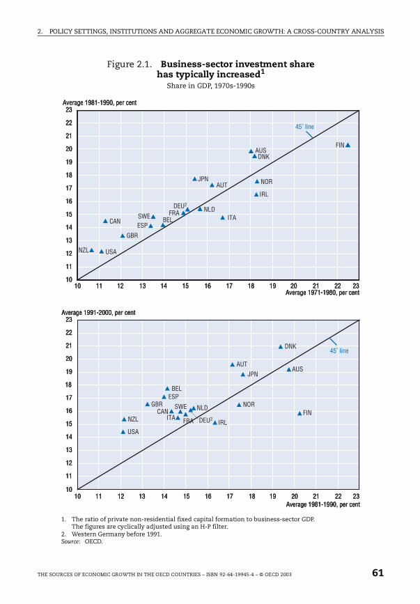
2. POLICY SETTINGS, INSTITUTIONS AND AGGREGATE ECONOMIC GROWTH: A CROSS-COUNTRY ANALYSIS
Figure 2.1. Business-sector investment share has typically increased1
Share in GDP, 1970s-1990s
1. The ratio of private non-residential fixed capital formation to business-sector GDP.The figures are cyclically adjusted using an H-P filter.
2. Western Germany before 1991.Source: OECD.
10
11
12
13
14
15
16
17
18
19
20
21
22
23
10
11
12
13
14
15
16
17
18
19
20
21
22
23
10 11 12 13 14 15 16 17 18 19 20 21 22 23
10 11 12 13 14 15 16 17 18 19 20 21 22 23
Average 1981-1990, per cent
Average 1971-1980, per cent
Average 1991-2000, per cent
Average 1981-1990, per cent
DEU2
USA
GBR
SWEESP
NOR
NZL
NLD
JPN
ITA
IRL
FRA
FIN
45˚ line
45˚ line
DNK
CAN BEL
AUT
AUS
DEU2
USA
GBR SWEESP
NOR
NZL
NLD
JPN
ITAIRLFRA
FIN
DNK
CAN
BEL
AUTAUS
10
11
12
13
14
15
16
17
18
19
20
21
22
23
10
11
12
13
14
15
16
17
18
19
20
21
22
23
10 11 12 13 14 15 16 17 18 19 20 21 22 23
10 11 12 13 14 15 16 17 18 19 20 21 22 23
Average 1981-1990, per cent
Average 1971-1980, per cent
Average 1991-2000, per cent
Average 1981-1990, per cent
DEU2
USA
GBR
SWEESP
NOR
NZL
NLD
JPN
ITA
IRL
FRA
FIN
45˚ line
45˚ line
DNK
CAN BEL
AUT
AUS
DEU2
USA
GBR SWEESP
NOR
NZL
NLD
JPN
ITAIRLFRA
FIN
DNK
CAN
BEL
AUTAUS
THE SOURCES OF ECONOMIC GROWTH IN THE OECD COUNTRIES – ISBN 92-64-19945-4 – © OECD 2003 61
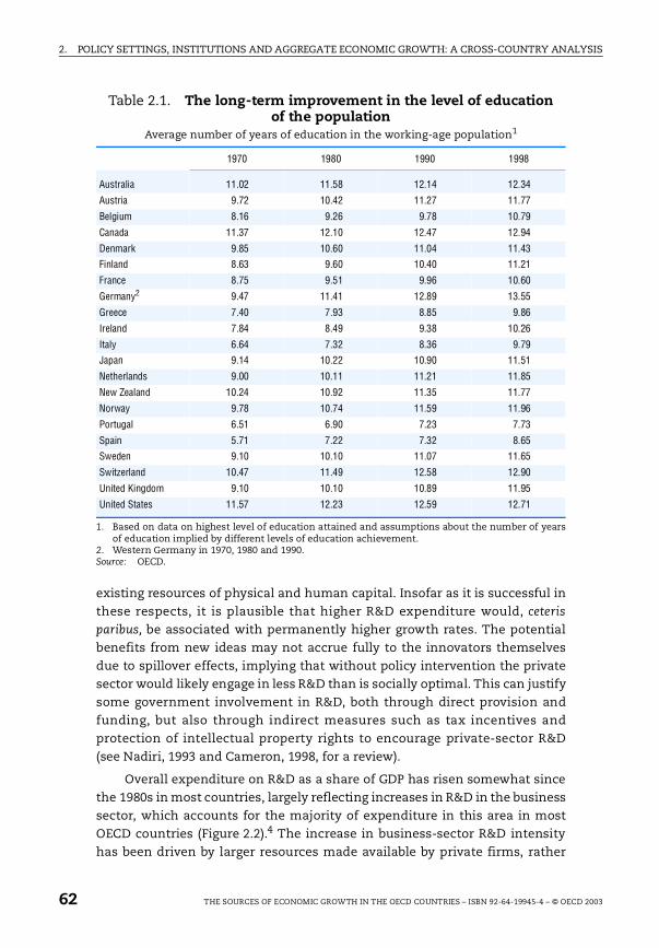
2. POLICY SETTINGS, INSTITUTIONS AND AGGREGATE ECONOMIC GROWTH: A CROSS-COUNTRY ANALYSIS
existing resources of physical and human capital. Insofar as it is successful inthese respects, it is plausible that higher R&D expenditure would, ceteris
paribus, be associated with permanently higher growth rates. The potentialbenefits from new ideas may not accrue fully to the innovators themselvesdue to spillover effects, implying that without policy intervention the privatesector would likely engage in less R&D than is socially optimal. This can justifysome government involvement in R&D, both through direct provision andfunding, but also through indirect measures such as tax incentives andprotection of intellectual property rights to encourage private-sector R&D(see Nadiri, 1993 and Cameron, 1998, for a review).
Overall expenditure on R&D as a share of GDP has risen somewhat sincethe 1980s in most countries, largely reflecting increases in R&D in the businesssector, which accounts for the majority of expenditure in this area in mostOECD countries (Figure 2.2).4 The increase in business-sector R&D intensityhas been driven by larger resources made available by private firms, rather
Table 2.1. The long-term improvement in the level of education of the population
Average number of years of education in the working-age population1
1. Based on data on highest level of education attained and assumptions about the number of yearsof education implied by different levels of education achievement.
2. Western Germany in 1970, 1980 and 1990.Source: OECD.
1970 1980 1990 1998
Australia 11.02 11.58 12.14 12.34
Austria 9.72 10.42 11.27 11.77
Belgium 8.16 9.26 9.78 10.79
Canada 11.37 12.10 12.47 12.94
Denmark 9.85 10.60 11.04 11.43
Finland 8.63 9.60 10.40 11.21
France 8.75 9.51 9.96 10.60
Germany2 9.47 11.41 12.89 13.55
Greece 7.40 7.93 8.85 9.86
Ireland 7.84 8.49 9.38 10.26
Italy 6.64 7.32 8.36 9.79
Japan 9.14 10.22 10.90 11.51
Netherlands 9.00 10.11 11.21 11.85
New Zealand 10.24 10.92 11.35 11.77
Norway 9.78 10.74 11.59 11.96
Portugal 6.51 6.90 7.23 7.73
Spain 5.71 7.22 7.32 8.65
Sweden 9.10 10.10 11.07 11.65
Switzerland 10.47 11.49 12.58 12.90
United Kingdom 9.10 10.10 10.89 11.95
United States 11.57 12.23 12.59 12.71
62 THE SOURCES OF ECONOMIC GROWTH IN THE OECD COUNTRIES – ISBN 92-64-19945-4 – © OECD 2003
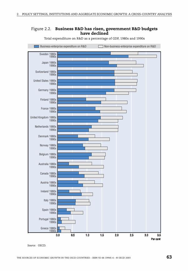
2. POLICY SETTINGS, INSTITUTIONS AND AGGREGATE ECONOMIC GROWTH: A CROSS-COUNTRY ANALYSIS
Figure 2.2. Business R&D has risen, government R&D budgets have declined
Total expenditure on R&D as a percentage of GDP, 1980s and 1990s
Source: OECD.
Business-enterprise expenditure on R&D Non-business-enterprise expenditure on R&D
3.02.50.0 0.5 1.0 1.5 2.0 3.5 1990s
Greece 1980s
1990sPortugal 1980s
1990sSpain 1980s
1990sItaly 1980s
1990sIreland 1980s
1990sAustria 1980s
1990sCanada 1980s
1990sAustralia 1980s
1990sBelgium 1980s
1990sNorway 1980s
1990sDenmark 1980s
1990sNetherlands 1980s
1990sUnited Kingdom 1980s
1990sFrance 1980s
1990sFinland 1980s
1990sGermany 1980s
1990sUnited States 1980s
1990sSwitzerland 1980s
1990sJapan 1980s
1990sSweden 1980s
Per cent
THE SOURCES OF ECONOMIC GROWTH IN THE OECD COUNTRIES – ISBN 92-64-19945-4 – © OECD 2003 63

2. POLICY SETTINGS, INSTITUTIONS AND AGGREGATE ECONOMIC GROWTH: A CROSS-COUNTRY ANALYSIS
than by governments: indeed the share of publicly-financed business-sector
R&D has declined over the past decade (see OECD, 2001d).
An important policy consideration is whether the relationship betweenpublic and private R&D is one of complementarity or substitution. Availableempirical literature gives conflicting answers: a number of studies support thecomplementarity hypothesis, but others cite instances where publicly-fundedR&D displaces private investment (see David et al., 1999 for a survey and Guellec
and van Pottelsberge, 2000). A final consideration with respect to the role ofpublic-sector R&D is that it is often directed at making improvements in areassuch as defence and medical research, where the impact on output growth couldbe diffused and slow to come about (see OECD, 1998). All in all, theseconsiderations suggest that when taking R&D activity into account as anadditional form of investment, the possible interactions between different formsof R&D expenditure and different forms of financing should also be considered.
Policy and institutional influences on growth
Macroeconomic policy setting and growth
In recent years most OECD countries have made significant steps towardslow inflation and improved public finances. A number of studies have shownthe effects for economic growth of these moves towards more stability-oriented macroeconomic policies to be beneficial, at least for a while. Threeissues have received particular attention: the benefits of maintaining low andstable inflation, the impact of government deficits on private investment, andthe possibility of negative impacts on growth stemming from a too-largegovernment sector (with the associated heavy tax burden to finance highgovernment expenditure).
Inflation and growth. The usual arguments for lower and more stableinflation rates include reduced uncertainty in the economy and enhancedefficiency of the price mechanism.5 To a certain extent, inflation can beconsidered as a tax on investment,6 so that low levels of inflation may reducethe profitability required to undertake an investment project, with an overall
positive impact on the accumulation of physical capital. On the other hand, alower rate of inflation may reduce the opportunity cost of holding money,thereby leading to a portfolio shift from capital to money and a decline ininvestment.7 However, this effect is probably very small because moneybalances are only a small fraction of the capital stock.
Inflation could also have an effect on capital accumulation via its impact
on economic uncertainty. A lower level of inflation may be associated withreduced uncertainty about inflation8 and reduced “noise” in price signals,reflected in a smaller amount of relative price variability.9 Reduced
64 THE SOURCES OF ECONOMIC GROWTH IN THE OECD COUNTRIES – ISBN 92-64-19945-4 – © OECD 2003
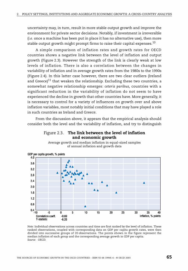
2. POLICY SETTINGS, INSTITUTIONS AND AGGREGATE ECONOMIC GROWTH: A CROSS-COUNTRY ANALYSIS
uncertainty may, in turn, result in more stable output growth and improve the
environment for private sector decisions. Notably, if investment is irreversible(i.e. once a machine has been put in place it has no alternative use), then morestable output growth might prompt firms to raise their capital expenses.10
A simple comparison of inflation rates and growth rates for OECDcountries shows a negative link between the level of inflation and outputgrowth (Figure 2.3). However the strength of the link is clearly weak at low
levels of inflation. There is also a correlation between the changes invariability of inflation and in average growth rates from the 1980s to the 1990s(Figure 2.4). In this latter case however, there are two clear outliers (Irelandand Greece)11 that weaken the relationship. Excluding these two countries, asomewhat negative relationship emerges: ceteris paribus, countries with asignificant reduction in the variability of inflation do not seem to haveexperienced the decline in growth that other countries have. More generally, itis necessary to control for a variety of influences on growth over and aboveinflation variables, most notably initial conditions that may have played a rolein such countries as Ireland and Greece.
From the discussion above, it appears that the empirical analysis shouldconsider both the level and the variability of inflation, and try to distinguish
Figure 2.3. The link between the level of inflation and economic growth
Average growth and median inflation in equal-sized samples of annual inflation and growth data
Note: Individual observations across countries and time are first ranked by the level of inflation. Theseranked observations, coupled with corresponding data on GDP per capita growth rates, were thendivided into successive groups of 20 observations. The points shown in the figure represent themedian inflation of each group and the corresponding average growth in GDP per capita.Source: OECD.
0.4
0.8
1.2
1.6
2.0
2.4
2.8
3.2
3.6
4.0
-10 0-5 10 15 25 355 20 30 40Inflation, % pointsCorrelation coeff.
T-statistic-0.69-6.26
GDP per capita growth, % points
0.4
0.8
1.2
1.6
2.0
2.4
2.8
3.2
3.6
4.0
-10 0-5 10 15 25 355 20 30 40Inflation, % pointsCorrelation coeff.
T-statistic-0.69-6.26
GDP per capita growth, % points
0.4
0.8
1.2
1.6
2.0
2.4
2.8
3.2
3.6
4.0
-10 0-5 10 15 25 355 20 30 40Inflation, % pointsCorrelation coeff.
T-statistic-0.69-6.26
GDP per capita growth, % points
THE SOURCES OF ECONOMIC GROWTH IN THE OECD COUNTRIES – ISBN 92-64-19945-4 – © OECD 2003 65
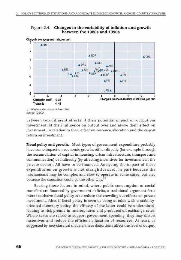
2. POLICY SETTINGS, INSTITUTIONS AND AGGREGATE ECONOMIC GROWTH: A CROSS-COUNTRY ANALYSIS
between two different effects: i) their potential impact on output via
investment; ii) their influence on output over and above their effect oninvestment, in relation to their effect on resource allocation and the ex-post
return on investment.
Fiscal policy and growth. Most types of government expenditure probablyhave some impact on economic growth, either directly (for example throughthe accumulation of capital in housing, urban infrastructure, transport and
communication) or indirectly (by affecting incentives for investment in theprivate sector). All have to be financed. Analysing the impact of theseexpenditures on growth is not straightforward, in part because themechanisms may be complex and slow to operate in some cases, but alsobecause the causation could go the other way.12
Bearing these factors in mind, where public consumption or social
transfers are financed by government deficits, a traditional argument for amore restrictive fiscal policy is to reduce the crowding out effects on privateinvestment. Also, if fiscal policy is seen as being at odds with a stability-oriented monetary policy, the efficacy of the latter could be undermined,leading to risk premia in interest rates and pressures on exchange rates.Where taxes are raised to support government spending, they may distortincentives and reduce the efficient allocation of resources. At least, assuggested by neo-classical models, these distortions affect the level of output.
Figure 2.4. Changes in the variability of inflation and growthbetween the 1980s and 1990s
1. Western Germany before 1991.Source: OECD.
-6 -5 -4 -3 -2 -1 0 1 2 3-3
-2
-1
0
1
2
3IRL
GRC
USA
SWE
NZL
NOR
NLD
JPN
ITAGBR
FRAFIN
ESP
DNK
CHE
CANBEL
AUSAUT
PRTDEU1
Change in average growth rate, per cent
Change in standard deviation of inflation, per centCorrelation coeff.T-statistic
-0.32-1.49
-6 -5 -4 -3 -2 -1 0 1 2 3-3
-2
-1
0
1
2
3IRL
GRC
USA
SWE
NZL
NOR
NLD
JPN
ITAGBR
FRAFIN
ESP
DNK
CHE
CANBEL
AUSAUT
PRTDEU1
Change in average growth rate, per cent
Change in standard deviation of inflation, per centCorrelation coeff.T-statistic
-0.32-1.49
-6 -5 -4 -3 -2 -1 0 1 2 3-3
-2
-1
0
1
2
3IRL
GRC
USA
SWE
NZL
NOR
NLD
JPN
ITAGBR
FRAFIN
ESP
DNK
CHE
CANBEL
AUSAUT
PRTDEU1
Change in average growth rate, per cent
Change in standard deviation of inflation, per centCorrelation coeff.T-statistic
-0.32-1.49
-6 -5 -4 -3 -2 -1 0 1 2 3-3
-2
-1
0
1
2
3IRL
GRC
USA
SWE
NZL
NOR
NLD
JPN
ITAGBR
FRAFIN
ESP
DNK
CHE
CANBEL
AUSAUT
PRTDEU1
Change in average growth rate, per cent
Change in standard deviation of inflation, per centCorrelation coeff.T-statistic
-0.32-1.49
-6 -5 -4 -3 -2 -1 0 1 2 3-3
-2
-1
0
1
2
3IRL
GRC
USA
SWE
NZL
NOR
NLD
JPN
ITAGBR
FRAFIN
ESP
DNK
CHE
CANBEL
AUSAUT
PRTDEU1
Change in average growth rate, per cent
Change in standard deviation of inflation, per centCorrelation coeff.T-statistic
-0.32-1.49
-6 -5 -4 -3 -2 -1 0 1 2 3-3
-2
-1
0
1
2
3IRL
GRC
USA
SWE
NZL
NOR
NLD
JPN
ITAGBR
FRAFIN
ESP
DNK
CHE
CANBEL
AUSAUT
PRTDEU1
Change in average growth rate, per cent
Change in standard deviation of inflation, per centCorrelation coeff.T-statistic
-0.32-1.49
66 THE SOURCES OF ECONOMIC GROWTH IN THE OECD COUNTRIES – ISBN 92-64-19945-4 – © OECD 2003
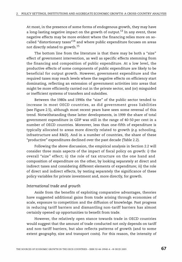
2. POLICY SETTINGS, INSTITUTIONS AND AGGREGATE ECONOMIC GROWTH: A CROSS-COUNTRY ANALYSIS
At most, in the presence of some forms of endogenous growth, they may have
a long-lasting negative impact on the growth of output.13 In any event, thesenegative effects may be more evident where the financing relies more on so-called “distortionary taxes”14 and where public expenditure focuses on areasnot directly related to growth.15
The bottom line from the literature is that there may be both a “size”effect of government intervention, as well as specific effects stemming from
the financing and composition of public expenditure. At a low level, theproductive effects of some components of public expenditure are likely to bebeneficial for output growth. However, government expenditure and therequired taxes may reach levels where the negative effects on efficiency startdominating, reflecting an extension of government activities into areas thatmight be more efficiently carried out in the private sector, and (or) misguidedor inefficient systems of transfers and subsidies.
Between the 1980s and 1990s the “size” of the public sector tended toincrease in most OECD countries, as did government gross liabilities(see Figure 2.5), although most recent years have seen some reversal of thistrend. Notwithstanding these latter developments, in 1999 the share of totalgovernment expenditure in GDP was still in the range of 40-50 per cent in anumber of OECD countries. Moreover, less than one-fifth of expenditure istypically allocated to areas more directly related to growth (e.g. schooling,infrastructure and R&D). And in a number of countries, the share of these“productive” expenditures declined over the past decade (Table 2.2).
Following the above discussion, the empirical analysis in Section 2.2 willconsider three main aspects of the impact of fiscal policy on growth: i) theoverall “size” effect; ii) the role of tax structure on the one hand andcomposition of expenditure on the other, by looking separately at direct andindirect taxes and considering different elements of expenditure; iii) the roleof direct and indirect effects, by testing separately the significance of thesepolicy variables for private investment and, more directly, for growth.
International trade and growth
Aside from the benefits of exploiting comparative advantages, theorieshave suggested additional gains from trade arising through economies ofscale, exposure to competition and the diffusion of knowledge. Past progressin reducing tariff barriers and dismantling non-tariff barriers has almostcertainly opened up opportunities to benefit from trade.
However, the relatively open stance towards trade in OECD countrieswould suggest that the amount of trade conducted not only depends on tariffand non-tariff barriers, but also reflects patterns of growth (and to someextent geography, size and transport costs). For this reason, the intensity of
THE SOURCES OF ECONOMIC GROWTH IN THE OECD COUNTRIES – ISBN 92-64-19945-4 – © OECD 2003 67
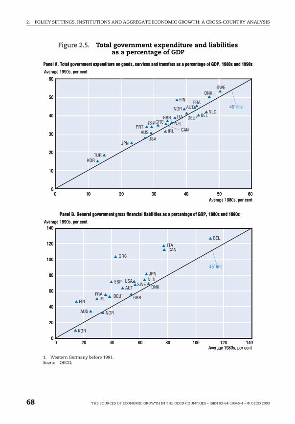
2. POLICY SETTINGS, INSTITUTIONS AND AGGREGATE ECONOMIC GROWTH: A CROSS-COUNTRY ANALYSIS
Figure 2.5. Total government expenditure and liabilities as a percentage of GDP
1. Western Germany before 1991.Source: OECD.
Panel A. Total government expenditure on goods, services and transfers as a percentage of GDP, 1980s and 1990s
Panel B. General government gross financial liabilities as a percentage of GDP, 1980s and 1990s
0
20
40
60
80
100
120
140
0 20 40 60 80 100 120 140
KOR
AUS
SWE
NOR
NLD
ISL
GRC
FIN
ESPDNK
BEL
AUT
CAN
GBR
ITA
FRA DEU1
JPN
USA
0
10
20
30
40
50
60
0 10 20 30 40 50 60
KOR
NZL
AUS
TUR
SWE
PRT
NORNLD
IRL
GRC
FIN
ESP
DNK
BEL
AUT
CAN
GBR ITA
FRA
DEU1
JPNUSA
45˚ line
45˚ line
Average 1980s, per cent
Average 1990s, per cent
Average 1990s, per cent
Average 1980s, per cent
68 THE SOURCES OF ECONOMIC GROWTH IN THE OECD COUNTRIES – ISBN 92-64-19945-4 – © OECD 2003
2.PO
LICY
SETT
ING
S, INST
ITU
TIO
NS A
ND
AG
GR
EGA
TE EC
ON
OM
IC G
RO
WT
H: A
CR
OSS-C
OU
NT
RY
AN
ALY
SIS
TH
E SOU
RC
ES OF EC
ON
OM
IC G
RO
WT
H IN
TH
E OEC
D C
OU
NT
RIES
– ISB
N 92-64-19945-4 – ©
OE
CD
200369
Table 2.2. Total government outlays and “productive” government spending as a share of total spending
A + B + CShare of total government outlays
in GDP
1985 1995 1985 1995 2000
26.8 23.6 38.0 35.7 32.614.1 13.0 50.3 52.5 47.922.3 . . 57.1 50.2 46.719.8 . . 45.2 45.0 37.716.4 15.9 54.23 56.6 49.915.7 14.4 51.9 53.5 51.016.0 12.9 45.6 46.3 43.323.6 22.4 35.3 39.2 38.515.9 18.0 50.7 38.0 29.318.8 14.5 49.7 51.1 44.4
. . . . 29.4 34.4 36.6
. . 30.4 17.6 19.3 23.1
. . . . 51.9 47.7 41.6
. . . . 51.86 38.6 38.620.2 21.3 41.5 47.6 40.812.9 19.0 39.9 41.3 40.815.8 17.1 39.7 44.0 38.8
. . . . 60.4 61.9 52.7
. . . . . . . . . .15.5 17.2 40.57 42.2 37.0
. . . . 33.8 32.9 29.9
Percentage
1. 1993 instead of 1995.2. 1992 instead of 1995.3. 1988.4. 1994.5. 1984.6. 1986.7. 1987.The concept of “productive” government spending is based on a taxonomy used by Barro (1991).Source: OECD.
A B C
Education Transport and communication R&D
1985 1995 1985 1995 1985 1995
Australia 14.6 13.2 10.1 8.3 2.15 2.24
Austria 9.6 9.5 3.3 2.1 1.2 1.4Belgium 12.7 . . 8.7 . . 0.9 . .Canada 13.0 . . 5.4 . . 1.5 . .Denmark 11.3 11.7 4.0 3.0 1.2 1.2France1 10.5 10.7 2.9 1.9 2.3 1.8Germany 9.5 7.6 4.3 3.4 2.2 1.8Iceland 13.0 12.3 9.0 7.6 1.6 2.5Ireland1 10.6 12.2 4.5 5.0 0.8 0.8Italy 10.0 8.9 7.7 4.6 1.2 1.0Japan 12.8 10.84 . . . . 1.8 1.9Korea 17.8 18.1 7.1 9.6 . . 2.7Netherlands 9.9 . . . . . . 1.8 . .New Zealand . . 13.34 . . . . . . 1.31
Norway 12.03 13.7 6.63 5.9 1.6 1.6Portugal2 8.7 13.3 3.6 4.8 0.55 0.9Spain 8.8 10.3 6.3 6.0 0.7 0.9Sweden . . . . . . . . 1.7 1.7Switzerland 19.7 . . 11.4 . . . . . .United Kingdom 10.2 12.1 3.2 3.6 2.0 1.5United States . . . . . . . . 4.1 2.8
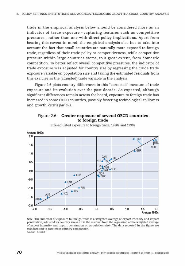
2. POLICY SETTINGS, INSTITUTIONS AND AGGREGATE ECONOMIC GROWTH: A CROSS-COUNTRY ANALYSIS
trade in the empirical analysis below should be considered more as an
indicator of trade exposure – capturing features such as competitivepressures – rather than one with direct policy implications. Apart frombearing this caveat in mind, the empirical analysis also has to take intoaccount the fact that small countries are naturally more exposed to foreigntrade, regardless of their trade policy or competitiveness, while competitivepressure within large countries stems, to a great extent, from domesticcompetition. To better reflect overall competitive pressures, the indicator oftrade exposure was adjusted for country size by regressing the crude tradeexposure variable on population size and taking the estimated residuals fromthis exercise as the (adjusted) trade variable in the analysis.
Figure 2.6 plots country differences in this “corrected” measure of tradeexposure and its evolution over the past decade. As expected, althoughsignificant differences remain across the board, exposure to foreign trade hasincreased in some OECD countries, possibly fostering technological spilloversand growth, ceteris paribus.
Figure 2.6. Greater exposure of several OECD countries to foreign trade
Size-adjusted exposure to foreign trade, 1980s and 1990s
Note: The indicator of exposure to foreign trade is a weighted average of export intensity and importpenetration, adjusted for country size (i.e it is the residual from the regression of the weighted averageof export intensity and import penetration on population size). The data reported in the figure arestandardised to ease cross-country comparison.Source: OECD.
-2.0
-1.5
-1.0
-0.5
0.0
0.5
1.0
1.5
2.0
-2.0 -1.5 -1.0 -0.5 0.0 0.5 1.0 2.01.5
USA
CHE
ESP
PRT
NOR
NZLJPN
ITAIRL
GRC
FIN
DNK
CAN
AUT
AUS
GBRNLD
BEL
SWEFRA
Average 1990s
45˚ line
Average 1980s
-2.0
-1.5
-1.0
-0.5
0.0
0.5
1.0
1.5
2.0
-2.0 -1.5 -1.0 -0.5 0.0 0.5 1.0 2.01.5
USA
CHE
ESP
PRT
NOR
NZLJPN
ITAIRL
GRC
FIN
DNK
CAN
AUT
AUS
GBRNLD
BEL
SWEFRA
Average 1990s
45˚ line
Average 1980s
-2.0
-1.5
-1.0
-0.5
0.0
0.5
1.0
1.5
2.0
-2.0 -1.5 -1.0 -0.5 0.0 0.5 1.0 2.01.5
USA
CHE
ESP
PRT
NOR
NZLJPN
ITAIRL
GRC
FIN
DNK
CAN
AUT
AUS
GBRNLD
BEL
SWEFRA
Average 1990s
45˚ line
Average 1980s
70 THE SOURCES OF ECONOMIC GROWTH IN THE OECD COUNTRIES – ISBN 92-64-19945-4 – © OECD 2003
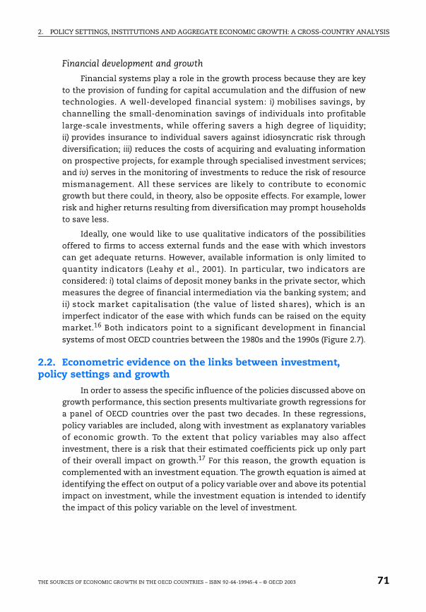
2. POLICY SETTINGS, INSTITUTIONS AND AGGREGATE ECONOMIC GROWTH: A CROSS-COUNTRY ANALYSIS
Financial development and growth
Financial systems play a role in the growth process because they are keyto the provision of funding for capital accumulation and the diffusion of newtechnologies. A well-developed financial system: i) mobilises savings, bychannelling the small-denomination savings of individuals into profitable
large-scale investments, while offering savers a high degree of liquidity;ii) provides insurance to individual savers against idiosyncratic risk throughdiversification; iii) reduces the costs of acquiring and evaluating informationon prospective projects, for example through specialised investment services;and iv) serves in the monitoring of investments to reduce the risk of resourcemismanagement. All these services are likely to contribute to economicgrowth but there could, in theory, also be opposite effects. For example, lowerrisk and higher returns resulting from diversification may prompt householdsto save less.
Ideally, one would like to use qualitative indicators of the possibilitiesoffered to firms to access external funds and the ease with which investorscan get adequate returns. However, available information is only limited toquantity indicators (Leahy et al., 2001). In particular, two indicators areconsidered: i) total claims of deposit money banks in the private sector, whichmeasures the degree of financial intermediation via the banking system; andii) stock market capitalisation (the value of listed shares), which is animperfect indicator of the ease with which funds can be raised on the equitymarket.16 Both indicators point to a significant development in financial
systems of most OECD countries between the 1980s and the 1990s (Figure 2.7).
2.2. Econometric evidence on the links between investment, policy settings and growth
In order to assess the specific influence of the policies discussed above ongrowth performance, this section presents multivariate growth regressions fora panel of OECD countries over the past two decades. In these regressions,policy variables are included, along with investment as explanatory variablesof economic growth. To the extent that policy variables may also affectinvestment, there is a risk that their estimated coefficients pick up only partof their overall impact on growth.17 For this reason, the growth equation iscomplemented with an investment equation. The growth equation is aimed atidentifying the effect on output of a policy variable over and above its potentialimpact on investment, while the investment equation is intended to identifythe impact of this policy variable on the level of investment.
THE SOURCES OF ECONOMIC GROWTH IN THE OECD COUNTRIES – ISBN 92-64-19945-4 – © OECD 2003 71
2. POLICY SETTINGS, INSTITUTIONS AND AGGREGATE ECONOMIC GROWTH: A CROSS-COUNTRY ANALYSIS
Figure 2.7. Significant developments in financial systemsPrivate credit of deposit money bank provided to the private sector
and stock market capitalisation as a percentage of the GDP, 1990 and 1997
Source: World Bank.
Panel A. Private credit by deposit money banks to GDP
Panel B. Stock market capitalisation to GDP
1997
1997
19900.0 0.2 0.4 0.6 0.8 1.0 1.2 1.4 1.6 1.8
0.0
0.2
0.4
0.6
0.8
1.0
1.2
1.4
1.6
1.8
GRCSWE
FIN
BELFRA
NZL
NLD JPN
GBR
45˚ line
45˚ line
CHE
DNK
ITA
USACANESP
AUS
DEU
NOR
AUT
0.0
0.2
0.4
0.6
0.8
1.0
1.2
1.4
1.6
0.0 0.2 0.4 0.6 0.8 1.0 1.2 1.4 1.6
AUTGRC
ITADEU
NOR BELFRAESP
DNKFIN JPN
CAN
NZL
SWE NLDUSA
CHE GBRAUS
1990
72 THE SOURCES OF ECONOMIC GROWTH IN THE OECD COUNTRIES – ISBN 92-64-19945-4 – © OECD 2003
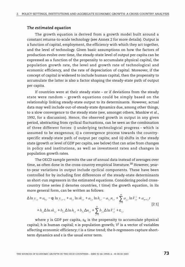
2. POLICY SETTINGS, INSTITUTIONS AND AGGREGATE ECONOMIC GROWTH: A CROSS-COUNTRY ANALYSIS
The estimated equation
The growth equation is derived from a growth model built around aconstant returns-to-scale technology (see Annex 2 for more details). Output isa function of capital, employment, the efficiency with which they act together,
and the level of technology. Given basic assumptions on how the factors ofproduction evolve over time, the steady-state level of output per capita can beexpressed as a function of the propensity to accumulate physical capital, thepopulation growth rate, the level and growth rate of technological andeconomic efficiency, and the rate of depreciation of capital. Moreover, if theconcept of capital is widened to include human capital, then the propensity toaccumulate the latter is also a factor shaping the steady-state path of outputper capita.
If countries were at their steady state – or if deviations from the steadystate were random – growth equations could be simply based on therelationship linking steady-state output to its determinants. However, actualdata may well include out-of-steady-state dynamics due, among other things,to a slow convergence to the steady state (see, amongst others, Mankiw et al.,1992, for a discussion). Hence, the observed growth in output in any givenperiod, abstracting from cyclical fluctuations, can be seen as the combinationof three different forces: i) underlying technological progress – which isassumed to be exogenous; ii) a convergence process towards the country-specific steady-state path of output per capita; and iii) shifts in the steady
state (growth or level of GDP per capita, see below) that can arise from changesin policy and institutions, as well as investment rates and changes inpopulation growth rates.
The OECD sample permits the use of annual data instead of averages overtime, as often done in the cross-country empirical literature.18 However, year-to-year variations in output include cyclical components. These have been
controlled for by including first differences of the steady-state determinantsas short-run regressors in the estimated equations. Considering pooled cross-country time series (i denotes countries, t time) the growth equation, in itsmore general form, can be written as follows:
where y is GDP per capita, sK is the propensity to accumulate physicalcapital; h is human capital; n is population growth; Vj is a vector of variablesaffecting economic efficiency; t is a time trend; the b-regressors capture short-
term dynamics and ε is the usual error term.
ti
m
j
j
tiijtiitiitii
im
m
j
j
tiijtiitiitiitiiiti
Vbnbhbskb
taVanahaskayay
,
4
,,,,3,,2,,1
,1
4
,,,,3,,2,,11,,0,
lnlnln
lnlnlnlnln
ε
φ
+∆+∆+∆+∆+
++−++−=∆
∑
∑
=
+=
−
[2.1]
THE SOURCES OF ECONOMIC GROWTH IN THE OECD COUNTRIES – ISBN 92-64-19945-4 – © OECD 2003 73
2. POLICY SETTINGS, INSTITUTIONS AND AGGREGATE ECONOMIC GROWTH: A CROSS-COUNTRY ANALYSIS
It should be stressed that equation [2.1] is a fairly general specification,
and different growth models are nested in it. The estimated parameters ofequation [2.1] allow distinguishing amongst some of these models. Inparticular, a significant coefficient on the lagged level of GDP per capita,i.e. the existence of convergence towards a country-specific steady state,would exclude one class of endogenous growth models (i.e. those à la Romer,1986)19. However, this would not be sufficient evidence to rule out otherendogenous models (e.g. à la Lucas, 1988).20 Indeed, even in the presence ofconvergence, a number of empirical papers have interpreted the estimatedpolicy coefficients as persistent growth effects.
The distinction between temporary or permanent growth effects mayseem somewhat semantic if the speed of convergence to the steady state isvery slow, as in most empirical studies focusing on a large set of countries.21
However, consistent with some recent studies focusing on panel data, theevidence provided below suggests a relatively rapid speed of convergence forthe OECD countries and thus, the choice between the two alternativeinterpretations of the results does matter in drawing policy conclusions. Theapproach used in this chapter is to consider the estimated coefficients asindicating temporary effects on growth due to the shift effect on the steady-
state path of output per capita.
For reasons discussed in Box 2.2, the econometric procedure chosen forestimating equation [2.1] is the Pooled Mean Group (PMG) approach, whichallows intercepts, the convergence parameter (φ), short-run coefficients (bs)and error variances to differ freely across countries, but imposes homogeneity
on long-run coefficients. A good argument can be made for common long-runcoefficients for the OECD countries, given that they have access to commontechnologies and have intensive inter-linkages through trade and foreigndirect investment, all factors contributing to lead to similar long-runproduction function parameters. With the PMG procedure, the followingrestricted version of equation [2.1] is estimated on pooled cross-country time-series data:
where the long-run coefficients as,i /φi = θs can now be read directly as the
parameters of factors affecting the steady state path of output per capita.
ti
m
j
j
tiijtiitiitii
m
m
j
j
tijtitititiiti
Vbnbhbskb
taVnhskyy
,
4
,,,,3,,2,,1
01
4
,,3,2,11,,
lnlnln
lnlnlnlnln
ε
θθθθθφ
+∆+∆+∆+∆+
−+−+−−−=∆
∑
∑
=
+=
−
[2.2]
74 THE SOURCES OF ECONOMIC GROWTH IN THE OECD COUNTRIES – ISBN 92-64-19945-4 – © OECD 2003
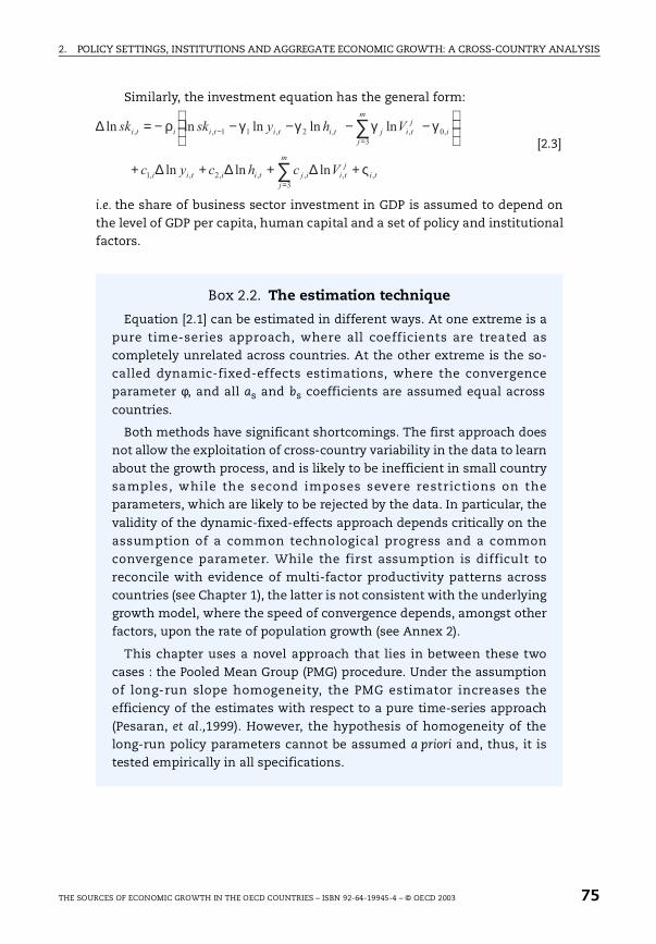
2. POLICY SETTINGS, INSTITUTIONS AND AGGREGATE ECONOMIC GROWTH: A CROSS-COUNTRY ANALYSIS
Similarly, the investment equation has the general form:
i.e. the share of business sector investment in GDP is assumed to depend onthe level of GDP per capita, human capital and a set of policy and institutionalfactors.
ti
m
j
j
tiijtiitii
i
m
j
j
tijtititiiti
Vchcyc
Vhysksk
,
3
,,,,2,,1
,0
3
,,2,11,,
lnlnln
lnlnlnlnln
ς
γγγγρ
+∆+∆+∆+
−−−−−=∆
∑
∑
=
=−
[2.3]
Box 2.2. The estimation technique
Equation [2.1] can be estimated in different ways. At one extreme is apure time-series approach, where all coefficients are treated ascompletely unrelated across countries. At the other extreme is the so-called dynamic-fixed-effects estimations, where the convergenceparameter φ, and all as and bs coefficients are assumed equal across
countries.
Both methods have significant shortcomings. The first approach doesnot allow the exploitation of cross-country variability in the data to learnabout the growth process, and is likely to be inefficient in small countrysamples, while the second imposes severe restrictions on theparameters, which are likely to be rejected by the data. In particular, the
validity of the dynamic-fixed-effects approach depends critically on theassumption of a common technological progress and a commonconvergence parameter. While the first assumption is difficult toreconcile with evidence of multi-factor productivity patterns acrosscountries (see Chapter 1), the latter is not consistent with the underlyinggrowth model, where the speed of convergence depends, amongst otherfactors, upon the rate of population growth (see Annex 2).
This chapter uses a novel approach that lies in between these twocases : the Pooled Mean Group (PMG) procedure. Under the assumptionof long-run slope homogeneity, the PMG estimator increases theefficiency of the estimates with respect to a pure time-series approach(Pesaran, et al.,1999). However, the hypothesis of homogeneity of thelong-run policy parameters cannot be assumed a priori and, thus, it istested empirically in all specifications.
THE SOURCES OF ECONOMIC GROWTH IN THE OECD COUNTRIES – ISBN 92-64-19945-4 – © OECD 2003 75
2. POLICY SETTINGS, INSTITUTIONS AND AGGREGATE ECONOMIC GROWTH: A CROSS-COUNTRY ANALYSIS
Regression results and interpretation
The growth equations are estimated for 21 OECD countries over theperiod 1971-1998.22 The countries are chosen because they have continuousannual series for most of the variables used in the growth equations over the
bulk of the period. Details on the variables used in the regression are inBox 2.3. This section presents the core results of the econometric analysis.Supplementary estimates, details on the model selection process for thedifferent specifications and sensitivity analysis can be found in Bassanini, et
al. (2001).
Consistent with the standard neo-classical growth model, the initial
specification only includes a convergence factor and the basic determinants ofthe steady state GDP per capita, namely the accumulation of physical capitaland population growth. The first extension involves the introduction ofhuman capital, while further extensions consider R&D and a set of policy andinstitutional factors potentially affecting economic efficiency.
The role of convergence and capital accumulation in the growth process
For various specifications (basic and extended) of the model, Table 2.3reports the estimated coefficients and implied parameters for the basicfactors driving the growth process, physical capital, human capital andconvergence. All specifications suggest a process of (conditional) convergence,supporting the specification adopted in equation [2.2]. Moreover, in allspecifications (whether basic or extended), both physical and human capitalappear to have a positive and significant effect on economic growth. There is,however, some variability in the estimated magnitude of their impact thatimplicitly underlines the importance of model specification. In particular,standard growth equations that do not control for human capital mayoverestimate the effect of accumulation of physical capital on growth, while atthe same time the model augmented with human capital yields an
implausibly high coefficient on (i.e. return from) this factor.
More stable and reasonable coefficients are obtained in the three right-hand-side columns of Table 2.3, which report specifications that furtheraugment the model with variables capturing framework conditions andpolicies. The estimated coefficients for physical capital are broadly consistentwith other growth studies: i.e. on average a 1 percentage point increase in the
investment share brings about an increase in steady-state GDP per capita ofabout 1.3 per cent.23 The coefficients on human capital still suggest relativelyhigh returns to education: the long-run effect on the level of GDP per capita ofone additional year of education (corresponding to a rise in human capital byabout 10 per cent) ranges between 4 and 7 per cent. These values contrastwith many studies that found no or very limited effects of human capital on
76 THE SOURCES OF ECONOMIC GROWTH IN THE OECD COUNTRIES – ISBN 92-64-19945-4 – © OECD 2003
2. POLICY SETTINGS, INSTITUTIONS AND AGGREGATE ECONOMIC GROWTH: A CROSS-COUNTRY ANALYSIS
Box 2.3. Description of the variables used in the empirical analysis
The baseline variables used in the regression include the followingexplanatory variables:
Dependent variable (∆logY). Growth in real GDP per head of populationaged 15-64 years expressed in (1993) Purchasing Power Parities (PPP);
Catch-up variable (logY–1). Lagged real GDP per head of populationaged 15-64 years, in PPP;
Physical capital accumulation (logSK). The propensity to accumulatephysical capital is proxied by the ratio of real private non-residentialfixed capital formation to real private GDP;1
Stock of human capital (logH) is proxied by the average number ofyears of schooling of the population from 25 to 64 years of age.2
Population growth (∆logP). Growth in population aged 15-64 years;
The auxiliary policy-related variables included in the augmentedgrowth regressions were as follows:
Measures of inflation: 1) the rate of growth of the private finalconsumption deflator (Infl); and 2) the standard deviation of the rate ofgrowth in private final consumption deflator (SDInfl) – estimated overa three-year period (t–1, t, t+1).
Indicators of government size and financing: 1) the ratio of generalgovernment current nominal tax and non-tax receipts in nominal GDP(logTax); 2) the ratio of direct to indirect tax receipts (log(Tax distr);3) the ratio of government nominal final consumption expenditure tonominal GDP (log(Gov cons)); and 4) the ratio of government real fixedcapital formation to real GDP (logSK
gov).
Measures of R&D intensity: 1) gross domestic expenditure on R&D as apercentage of GDP (logR&Dtot)); 2) business sector expenditure on R&Das a percentage of GDP (logBERD); and 3) the percentage of BERDfinanced by industry (logBERDind).
Indicators measuring financial development: 1) private credit of depositmoney banks provided to the private sector as a percentage of GDP
(logPCB); and 2) stock market capitalisation as a percentage of GDP(logSMC).3
THE SOURCES OF ECONOMIC GROWTH IN THE OECD COUNTRIES – ISBN 92-64-19945-4 – © OECD 2003 77
2. POLICY SETTINGS, INSTITUTIONS AND AGGREGATE ECONOMIC GROWTH: A CROSS-COUNTRY ANALYSIS
growth (see for example, Benhabib and Spiegel, 1994; Barro and Sala-i-Martin,
1995). As pointed out by Bassanini and Scarpetta (2001), better data qualityand a more appropriate econometric procedure are likely to account for theencouraging results on human capital reported in Table 2.3.24 It should also bestressed that the present estimates are broadly consistent with estimatedreturns to schooling in the microeconomic literature (see Psacharopoulos,1994).
The magnitude of the impact of human capital on growth found in thisanalysis might be interpreted as suggesting that the economy-wide returns toinvestment in education may be larger than those experienced by individuals.If this were the case, it could be through spillover effects such as links betweeneducation levels and advances in technology, through which human capitalmay not only affect the level of long-run output per capita, but may also havemore persistent effects on growth. In the presence of such spillovers,
Box 2.3. Description of the variables used in the empirical analysis (cont.)
Indicators of the exposure of countries to foreign trade: a weighted averageof export intensity and import penetration.4 In the empirical analysisthis measure was adjusted for country size (log(Trade exp)adj). It wasachieved by regressing the crude trade exposure variable onpopulation size and taking the estimated residuals from this exerciseas the adjusted trade exposure.
All the auxiliary policy-related variables, with the exception of thoserelated to R&D, have been introduced with a lag to better identify theirimpact on output. See Bassanini et al. (2001) for the discussion of thisissue.
1. In the extended models, also government fixed capital formation is considered, but itsimpact on growth is allowed to differ from that of private fixed capital formation.
2. As discussed in Annex 2, growth regressions have often used enrolment rates from UNsources instead of education attainment, because the former are closer to the concept ofinvestment in human capital. However, changes in enrolment rates are likely to have animpact of GDP per capita growth only with a long lag: in a model with annual data and withrelatively limited time series (25-27 observations) there are inherent limits to the number oflags to be included in the specification. Moreover, a number of authors have questioned theuse of enrolment rates as a proxy for the concept of human capital that influence decisionsabout fertility, participation and so on (see amongst others, Barro and Lee, 1996). There isalso a practical issue that suggests using level data instead of first differences. Although thetime series on human capital used in this study have been checked for consistency ofdefinition over time (also on the basis of the work by de la Fuente and Doménech, 2000),they are often linear interpolations from five-year observations which make annualchanges potentially misleading.
3. See Leahy et al. (2001) for more details on the pros and cons of these two indicators.4. The index of trade exposure is calculated as follows: Trade Exp = Xi + (1 – Xi)*Mp, where Xi is
the ratio of exports to GDP and Mp is the ratio of imports to apparent consumption(domestic production minus exports plus imports).
78 THE SOURCES OF ECONOMIC GROWTH IN THE OECD COUNTRIES – ISBN 92-64-19945-4 – © OECD 2003
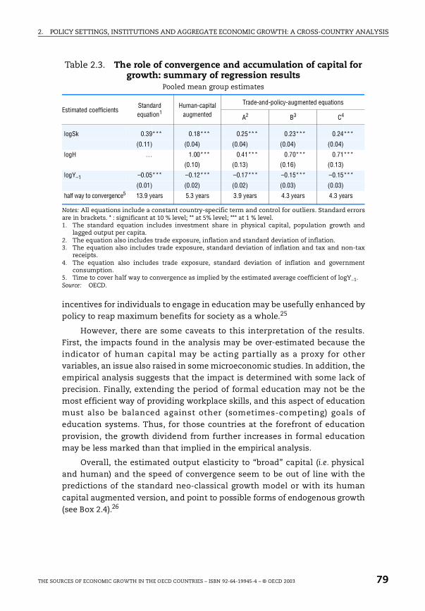
2. POLICY SETTINGS, INSTITUTIONS AND AGGREGATE ECONOMIC GROWTH: A CROSS-COUNTRY ANALYSIS
incentives for individuals to engage in education may be usefully enhanced bypolicy to reap maximum benefits for society as a whole.25
However, there are some caveats to this interpretation of the results.First, the impacts found in the analysis may be over-estimated because theindicator of human capital may be acting partially as a proxy for othervariables, an issue also raised in some microeconomic studies. In addition, theempirical analysis suggests that the impact is determined with some lack ofprecision. Finally, extending the period of formal education may not be themost efficient way of providing workplace skills, and this aspect of educationmust also be balanced against other (sometimes-competing) goals ofeducation systems. Thus, for those countries at the forefront of education
provision, the growth dividend from further increases in formal educationmay be less marked than that implied in the empirical analysis.
Overall, the estimated output elasticity to “broad” capital (i.e. physicaland human) and the speed of convergence seem to be out of line with thepredictions of the standard neo-classical growth model or with its human
capital augmented version, and point to possible forms of endogenous growth(see Box 2.4).26
Table 2.3. The role of convergence and accumulation of capital for growth: summary of regression results
Pooled mean group estimates
Notes: All equations include a constant country-specific term and control for outliers. Standard errorsare in brackets. * : significant at 10 % level; ** at 5% level; *** at 1 % level.1. The standard equation includes investment share in physical capital, population growth and
lagged output per capita.2. The equation also includes trade exposure, inflation and standard deviation of inflation.3. The equation also includes trade exposure, standard deviation of inflation and tax and non-tax
receipts.4. The equation also includes trade exposure, standard deviation of inflation and government
consumption.5. Time to cover half way to convergence as implied by the estimated average coefficient of logY–1.Source: OECD.
Estimated coefficientsStandard equation1
Human-capital augmented
Trade-and-policy-augmented equations
A2 B3 C4
logSk 0.39*** 0.18*** 0.25*** 0.23*** 0.24***
(0.11) (0.04) (0.04) (0.04) (0.04)
logH … 1.00*** 0.41*** 0.70*** 0.71***
(0.10) (0.13) (0.16) (0.13)
logY–1 –0.05*** –0.12*** –0.17*** –0.15*** –0.15***
(0.01) (0.02) (0.02) (0.03) (0.03)
half way to convergence5 13.9 years 5.3 years 3.9 years 4.3 years 4.3 years
THE SOURCES OF ECONOMIC GROWTH IN THE OECD COUNTRIES – ISBN 92-64-19945-4 – © OECD 2003 79
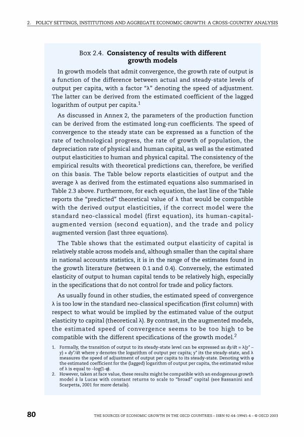
2. POLICY SETTINGS, INSTITUTIONS AND AGGREGATE ECONOMIC GROWTH: A CROSS-COUNTRY ANALYSIS
Box 2.4. Consistency of results with different growth models
In growth models that admit convergence, the growth rate of output isa function of the difference between actual and steady-state levels ofoutput per capita, with a factor “λ” denoting the speed of adjustment.The latter can be derived from the estimated coefficient of the laggedlogarithm of output per capita.1
As discussed in Annex 2, the parameters of the production functioncan be derived from the estimated long-run coefficients. The speed ofconvergence to the steady state can be expressed as a function of therate of technological progress, the rate of growth of population, thedepreciation rate of physical and human capital, as well as the estimatedoutput elasticities to human and physical capital. The consistency of theempirical results with theoretical predictions can, therefore, be verified
on this basis. The Table below reports elasticities of output and theaverage λ as derived from the estimated equations also summarised inTable 2.3 above. Furthermore, for each equation, the last line of the Tablereports the “predicted” theoretical value of λ that would be compatiblewith the derived output elasticities, if the correct model were thestandard neo-classical model (first equation), its human-capital-augmented version (second equation), and the trade and policyaugmented version (last three equations).
The Table shows that the estimated output elasticity of capital isrelatively stable across models and, although smaller than the capital sharein national accounts statistics, it is in the range of the estimates found inthe growth literature (between 0.1 and 0.4). Conversely, the estimatedelasticity of output to human capital tends to be relatively high, especiallyin the specifications that do not control for trade and policy factors.
As usually found in other studies, the estimated speed of convergenceλ is too low in the standard neo-classical specification (first column) withrespect to what would be implied by the estimated value of the outputelasticity to capital (theoretical λ). By contrast, in the augmented models,the estimated speed of convergence seems to be too high to becompatible with the different specifications of the growth model.2
1. Formally, the transition of output to its steady-state level can be expressed as dy/dt = λ(y* –y) + dy*/dt where y denotes the logarithm of output per capita; y* its the steady-state, and λmeasures the speed of adjustment of output per capita to its steady-state. Denoting with φthe estimated coefficient for the (lagged) logarithm of output per capita, the estimated valueof λ is equal to –log(1-φ).
2. However, taken at face value, these results might be compatible with an endogenous growthmodel à la Lucas with constant returns to scale to “broad” capital (see Bassanini andScarpetta, 2001 for more details).
80 THE SOURCES OF ECONOMIC GROWTH IN THE OECD COUNTRIES – ISBN 92-64-19945-4 – © OECD 2003
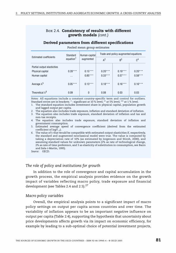
2. POLICY SETTINGS, INSTITUTIONS AND AGGREGATE ECONOMIC GROWTH: A CROSS-COUNTRY ANALYSIS
The role of policy and institutions for growth
In addition to the role of convergence and capital accumulation in thegrowth process, the empirical analysis provides evidence on the growthimpact of variables reflecting macro policy, trade exposure and financialdevelopment (see Tables 2.4 and 2.5).27
Macro policy variables
Overall, the empirical analysis points to a significant impact of macropolicy settings on output per capita across countries and over time. Thevariability of inflation appears to be an important negative influence onoutput per capita (Table 2.4), supporting the hypothesis that uncertainty aboutprice developments affects growth via its impact on economic efficiency, forexample by leading to a sub-optimal choice of potential investment projects,
Box 2.4. Consistency of results with different growth models (cont.)
Derived parameters from different specificationsPooled mean group estimates
Notes: All equations include a constant country-specific term and control for outliers.Standard errors are in brackets. * : significant at 10 % level; ** at 5% level; *** at 1 % level.1. The standard equation includes investment share in physical capital, population growth
and lagged output per capita.2. The equation also includes trade exposure, inflation and standard deviation of inflation.3. The equation also includes trade exposure, standard deviation of inflation and tax and
non-tax receipts.4. The equation also includes trade exposure, standard deviation of inflation and
government consumption.5. Estimated average speed of convergence coefficient (derived from the estimated
coefficient of logY–1).6. The value of λ that would be compatible with estimated output elasticities if, respectively,
the standard and augmented neoclassical model were true. The value is computed bytaking a depreciation rate of 10% (as estimated by Jorgenson and Stiroh, 2000), andassuming standard values for unknown parameters (2% as rate of technological change,2% as rate of time preference, and 3 as elasticity of substitution in consumption, see Barroand Sala-i-Martin, 1995).
Source: OECD.
Estimated coefficientsStandard equation1
Human-capital augmented
Trade-and-policy-augmented equations
A2 B3 C4
Partial output elasticities
Physical capital 0.28*** 0.15*** 0.20*** 0.19*** 0.20***
Human capital … 0.85*** 0.33*** 0.57*** 0.58***
Average λ5 0.05*** 0.13*** 0.18*** 0.16*** 0.16***
Theoretical λ6 0.09 0 0.08 0.03 0.03
THE SOURCES OF ECONOMIC GROWTH IN THE OECD COUNTRIES – ISBN 92-64-19945-4 – © OECD 2003 81
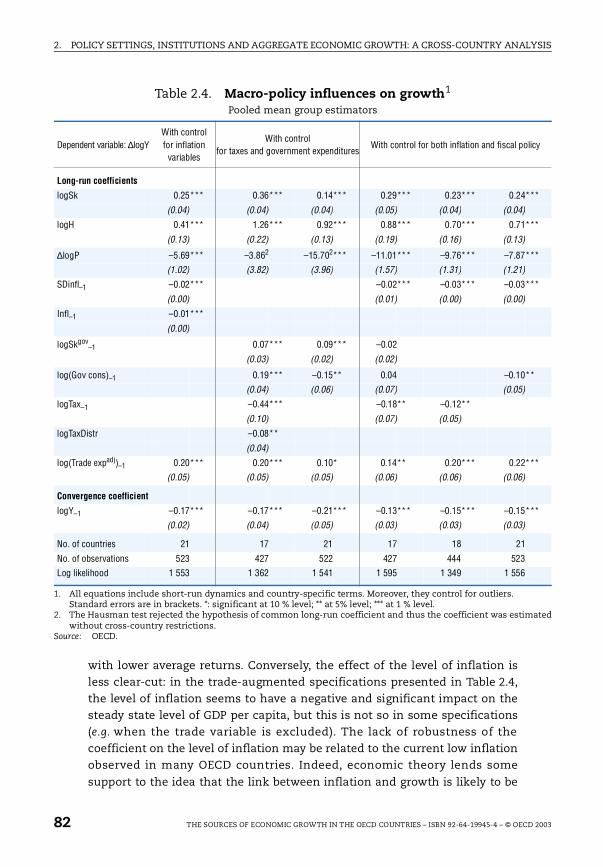
2. POLICY SETTINGS, INSTITUTIONS AND AGGREGATE ECONOMIC GROWTH: A CROSS-COUNTRY ANALYSIS
ated
icy
**
**
**
**
*
**
**
with lower average returns. Conversely, the effect of the level of inflation isless clear-cut: in the trade-augmented specifications presented in Table 2.4,the level of inflation seems to have a negative and significant impact on thesteady state level of GDP per capita, but this is not so in some specifications(e.g. when the trade variable is excluded). The lack of robustness of thecoefficient on the level of inflation may be related to the current low inflationobserved in many OECD countries. Indeed, economic theory lends some
support to the idea that the link between inflation and growth is likely to be
Table 2.4. Macro-policy influences on growth1
Pooled mean group estimators
1. All equations include short-run dynamics and country-specific terms. Moreover, they control for outliers.Standard errors are in brackets. *: significant at 10 % level; ** at 5% level; *** at 1 % level.
2. The Hausman test rejected the hypothesis of common long-run coefficient and thus the coefficient was estimwithout cross-country restrictions.
Source: OECD.
Dependent variable: ∆logYWith control for inflation
variables
With control for taxes and government expenditures
With control for both inflation and fiscal pol
Long-run coefficients
logSk 0.25*** 0.36*** 0.14*** 0.29*** 0.23*** 0.24*
(0.04) (0.04) (0.04) (0.05) (0.04) (0.04)
logH 0.41*** 1.26*** 0.92*** 0.88*** 0.70*** 0.71*
(0.13) (0.22) (0.13) (0.19) (0.16) (0.13)
∆logP –5.69*** –3.862 –15.702*** –11.01*** –9.76*** –7.87*
(1.02) (3.82) (3.96) (1.57) (1.31) (1.21)
SDinfl–1 –0.02*** –0.02*** –0.03*** –0.03*
(0.00) (0.01) (0.00) (0.00)
Infl–1 –0.01***
(0.00)
logSkgov–1 0.07*** 0.09*** –0.02
(0.03) (0.02) (0.02)
log(Gov cons)–1 0.19*** –0.15** 0.04 –0.10*
(0.04) (0.06) (0.07) (0.05)
logTax–1 –0.44*** –0.18** –0.12**
(0.10) (0.07) (0.05)
logTaxDistr –0.08**
(0.04)
log(Trade expadj)–1 0.20*** 0.20*** 0.10* 0.14** 0.20*** 0.22*
(0.05) (0.05) (0.05) (0.06) (0.06) (0.06)
Convergence coefficient
logY–1 –0.17*** –0.17*** –0.21*** –0.13*** –0.15*** –0.15*
(0.02) (0.04) (0.05) (0.03) (0.03) (0.03)
No. of countries 21 17 21 17 18 21
No. of observations 523 427 522 427 444 523
Log likelihood 1 553 1 362 1 541 1 595 1 349 1 556
82 THE SOURCES OF ECONOMIC GROWTH IN THE OECD COUNTRIES – ISBN 92-64-19945-4 – © OECD 2003
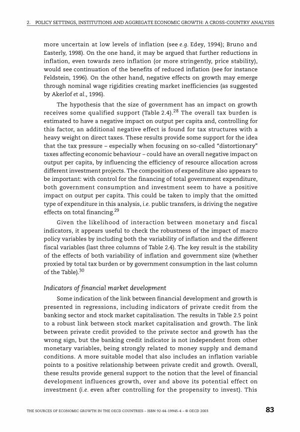
2. POLICY SETTINGS, INSTITUTIONS AND AGGREGATE ECONOMIC GROWTH: A CROSS-COUNTRY ANALYSIS
more uncertain at low levels of inflation (see e.g. Edey, 1994); Bruno and
Easterly, 1998). On the one hand, it may be argued that further reductions ininflation, even towards zero inflation (or more stringently, price stability),would see continuation of the benefits of reduced inflation (see for instanceFeldstein, 1996). On the other hand, negative effects on growth may emergethrough nominal wage rigidities creating market inefficiencies (as suggestedby Akerlof et al., 1996).
The hypothesis that the size of government has an impact on growthreceives some qualified support (Table 2.4).28 The overall tax burden isestimated to have a negative impact on output per capita and, controlling forthis factor, an additional negative effect is found for tax structures with aheavy weight on direct taxes. These results provide some support for the ideathat the tax pressure – especially when focusing on so-called “distortionary”taxes affecting economic behaviour – could have an overall negative impact onoutput per capita, by influencing the efficiency of resource allocation acrossdifferent investment projects. The composition of expenditure also appears tobe important: with control for the financing of total government expenditure,both government consumption and investment seem to have a positiveimpact on output per capita. This could be taken to imply that the omitted
type of expenditure in this analysis, i.e. public transfers, is driving the negativeeffects on total financing.29
Given the likelihood of interaction between monetary and fiscalindicators, it appears useful to check the robustness of the impact of macropolicy variables by including both the variability of inflation and the different
fiscal variables (last three columns of Table 2.4). The key result is the stabilityof the effects of both variability of inflation and government size (whetherproxied by total tax burden or by government consumption in the last columnof the Table).30
Indicators of financial market development
Some indication of the link between financial development and growth is
presented in regressions, including indicators of private credit from thebanking sector and stock market capitalisation. The results in Table 2.5 pointto a robust link between stock market capitalisation and growth. The linkbetween private credit provided to the private sector and growth has thewrong sign, but the banking credit indicator is not independent from othermonetary variables, being strongly related to money supply and demandconditions. A more suitable model that also includes an inflation variablepoints to a positive relationship between private credit and growth. Overall,these results provide general support to the notion that the level of financialdevelopment influences growth, over and above its potential effect oninvestment (i.e. even after controlling for the propensity to invest). This
THE SOURCES OF ECONOMIC GROWTH IN THE OECD COUNTRIES – ISBN 92-64-19945-4 – © OECD 2003 83
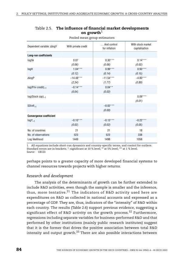
2. POLICY SETTINGS, INSTITUTIONS AND AGGREGATE ECONOMIC GROWTH: A CROSS-COUNTRY ANALYSIS
perhaps points to a greater capacity of more developed financial systems tochannel resources towards projects with higher returns.
Research and development
The analysis of the determinants of growth can be further extended toinclude R&D activities, even though the sample is smaller and the inference,thus, more tentative.31 The indicators of R&D activity used here are
expenditures on R&D as collected in national accounts and expressed as apercentage of GDP. They are, thus, indicators of the “intensity” of R&D withineach country. The results (Table 2.6) support previous evidence, suggesting asignificant effect of R&D activity on the growth process.32 Furthermore,regressions including separate variables for business-performed R&D and thatperformed by other institutions (mainly public research institutes) suggestthat it is the former that drives the positive association between total R&Dintensity and output growth.33 There are also possible interactions between
Table 2.5. The influence of financial market developments on growth1
Pooled mean group estimators
1. All equations include short-run dynamics and country-specific terms, and control for outliers.Standard errors are in brackets. *: significant at 10 % level; ** at 5% level; *** at 1 % level.Source: OECD.
Dependent variable: ∆logY With private credit… And control
for inflationWith stock market
capitalisation
Long-run coefficients
logSk 0.07 0.30*** 0.14***
(0.06) (0.06) (0.02)
logH 1.04*** 0.99*** 0.93***
(0.12) (0.14) (0.15)
∆logP –14.48*** –11.54*** –4.80***
(2.34) (1.77) (0.89)
log(Priv credit)–1 –0.14*** 0.04**
(0.04) (0.02)
log(Stock cap)–1 0.09***
(0.01)
SDinfl–1 –0.02***
(0.00)
Convergence coefficient
logY–1 –0.10*** –0.13*** –0.22***
(0.02) (0.02) (0.05)
No. of countries 21 21 18
No. of observations 523 523 338
Log likelihood 1449 1498 1058
84 THE SOURCES OF ECONOMIC GROWTH IN THE OECD COUNTRIES – ISBN 92-64-19945-4 – © OECD 2003
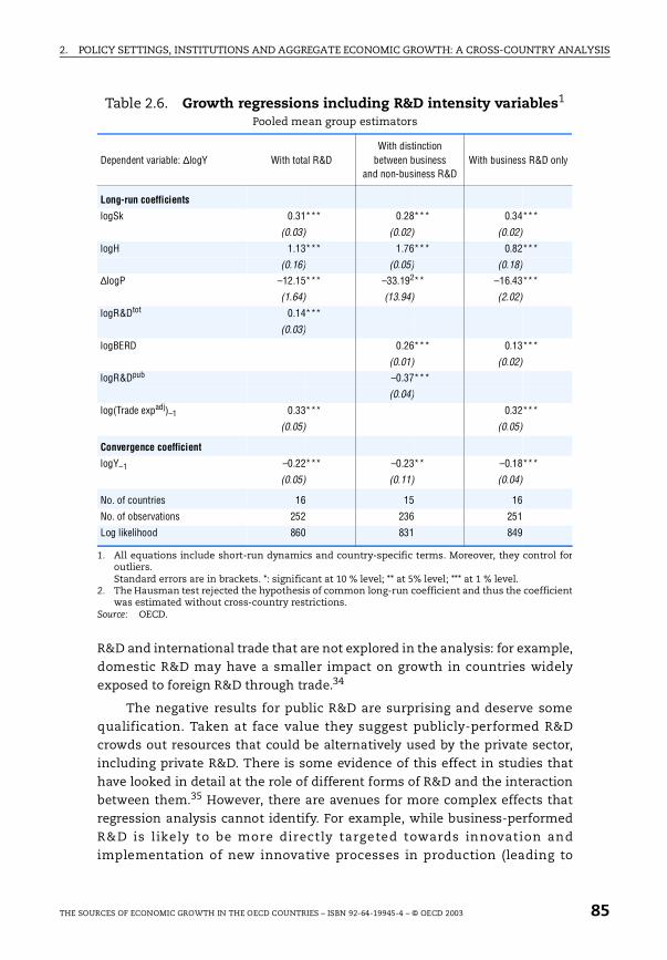
2. POLICY SETTINGS, INSTITUTIONS AND AGGREGATE ECONOMIC GROWTH: A CROSS-COUNTRY ANALYSIS
R&D and international trade that are not explored in the analysis: for example,domestic R&D may have a smaller impact on growth in countries widelyexposed to foreign R&D through trade.34
The negative results for public R&D are surprising and deserve somequalification. Taken at face value they suggest publicly-performed R&Dcrowds out resources that could be alternatively used by the private sector,including private R&D. There is some evidence of this effect in studies thathave looked in detail at the role of different forms of R&D and the interactionbetween them.35 However, there are avenues for more complex effects thatregression analysis cannot identify. For example, while business-performedR&D is likely to be more directly targeted towards innovation andimplementation of new innovative processes in production (leading to
Table 2.6. Growth regressions including R&D intensity variables1
Pooled mean group estimators
1. All equations include short-run dynamics and country-specific terms. Moreover, they control foroutliers.Standard errors are in brackets. *: significant at 10 % level; ** at 5% level; *** at 1 % level.
2. The Hausman test rejected the hypothesis of common long-run coefficient and thus the coefficientwas estimated without cross-country restrictions.
Source: OECD.
Dependent variable: ∆logY With total R&DWith distinction
between business and non-business R&D
With business R&D only
Long-run coefficients
logSk 0.31*** 0.28*** 0.34***
(0.03) (0.02) (0.02)
logH 1.13*** 1.76*** 0.82***
(0.16) (0.05) (0.18)
∆logP –12.15*** –33.192** –16.43***
(1.64) (13.94) (2.02)
logR&Dtot 0.14***
(0.03)
logBERD 0.26*** 0.13***
(0.01) (0.02)
logR&Dpub –0.37***
(0.04)
log(Trade expadj)–1 0.33*** 0.32***
(0.05) (0.05)
Convergence coefficient
logY–1 –0.22*** –0.23** –0.18***
(0.05) (0.11) (0.04)
No. of countries 16 15 16
No. of observations 252 236 251
Log likelihood 860 831 849
THE SOURCES OF ECONOMIC GROWTH IN THE OECD COUNTRIES – ISBN 92-64-19945-4 – © OECD 2003 85
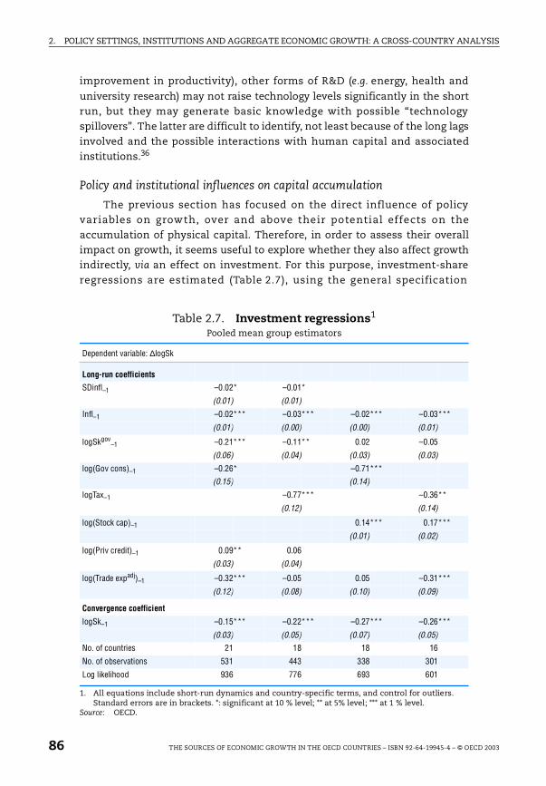
2. POLICY SETTINGS, INSTITUTIONS AND AGGREGATE ECONOMIC GROWTH: A CROSS-COUNTRY ANALYSIS
improvement in productivity), other forms of R&D (e.g. energy, health and
university research) may not raise technology levels significantly in the shortrun, but they may generate basic knowledge with possible “technologyspillovers”. The latter are difficult to identify, not least because of the long lagsinvolved and the possible interactions with human capital and associatedinstitutions.36
Policy and institutional influences on capital accumulation
The previous section has focused on the direct influence of policyvariables on growth, over and above their potential effects on theaccumulation of physical capital. Therefore, in order to assess their overallimpact on growth, it seems useful to explore whether they also affect growthindirectly, via an effect on investment. For this purpose, investment-shareregressions are estimated (Table 2.7), using the general specification
Table 2.7. Investment regressions1
Pooled mean group estimators
1. All equations include short-run dynamics and country-specific terms, and control for outliers.Standard errors are in brackets. *: significant at 10 % level; ** at 5% level; *** at 1 % level.
Source: OECD.
Dependent variable: ∆logSk
Long-run coefficients
SDinfl–1 –0.02* –0.01*
(0.01) (0.01)
Infl–1 –0.02*** –0.03*** –0.02*** –0.03***
(0.01) (0.00) (0.00) (0.01)
logSkgov–1 –0.21*** –0.11** 0.02 –0.05
(0.06) (0.04) (0.03) (0.03)
log(Gov cons)–1 –0.26* –0.71***
(0.15) (0.14)
logTax–1 –0.77*** –0.36**
(0.12) (0.14)
log(Stock cap)–1 0.14*** 0.17***
(0.01) (0.02)
log(Priv credit)–1 0.09** 0.06
(0.03) (0.04)
log(Trade expadj)–1 –0.32*** –0.05 0.05 –0.31***
(0.12) (0.08) (0.10) (0.09)
Convergence coefficient
logSk–1 –0.15*** –0.22*** –0.27*** –0.26***
(0.03) (0.05) (0.07) (0.05)
No. of countries 21 18 18 16
No. of observations 531 443 338 301
Log likelihood 936 776 693 601
86 THE SOURCES OF ECONOMIC GROWTH IN THE OECD COUNTRIES – ISBN 92-64-19945-4 – © OECD 2003
2. POLICY SETTINGS, INSTITUTIONS AND AGGREGATE ECONOMIC GROWTH: A CROSS-COUNTRY ANALYSIS
presented in equation [2.3] above.37 Overall, judging from these results and
those of the previous section, three main policy and institutional variablesseem to influence growth, both directly and indirectly: inflation, the “size” ofthe government and financial development.
In contrast with the results from the growth equation, the negative effectof the level of inflation is more significant than that of its variability ininvestment regressions. This finding is consistent with the view that
uncertainty about inflation, as captured by its variability, mainly influencesgrowth via distortion in the allocation of resources (as discussed above), ratherthan by discouraging the accumulation of physical capital, while high levels ofinflation indeed discourage savings and investment. There is also evidencethat the “size” of government may be negatively associated with the rate ofaccumulation of private capital, as can be seen by looking at the coefficients ofthe two proxies (taxes or government consumption in the specificationwithout taxes).
Finally, financial development might positively affect investment. As in thegrowth regressions, the indicator of credit provided by the banking sectorappears to be only weakly associated with investment, while the stock marketcapitalisation has a stronger effect.38 These results are consistent with a numberof empirical studies attempting to explain cross-country differences in growthacross a broad range of countries (including OECD and non-OECD economies),which have concluded that financial development plays a significant role (see,for example, Levine, 1997; Levine et al., 2000; Temple, 1999).
2.3. Assessing the long-run effects of policy and institutional changes on GDP per capita
The results of the previous section can be used to assess the effect of agiven change in a policy or institutional variable on steady-state output per
capita. Two important caveats need to be borne in mind in this exercise. First,as discussed above, it has been assumed that the policy and institutionalvariables affect only the level of economic efficiency and not its steady-stategrowth rate: the magnitude of the growth effects of some policy changes may,therefore, be underestimated. Second, the calculations should only be takenas broad indications, given the variability of coefficients across thespecifications and interaction effects between variables that may beimportant but cannot be taken into account.
Bearing in mind the illustrative nature of this exercise, the estimateddirect effects – derived from the growth equations that control for the level ofinvestment and indirect effects – derived by combining the effect on investment
THE SOURCES OF ECONOMIC GROWTH IN THE OECD COUNTRIES – ISBN 92-64-19945-4 – © OECD 2003 87
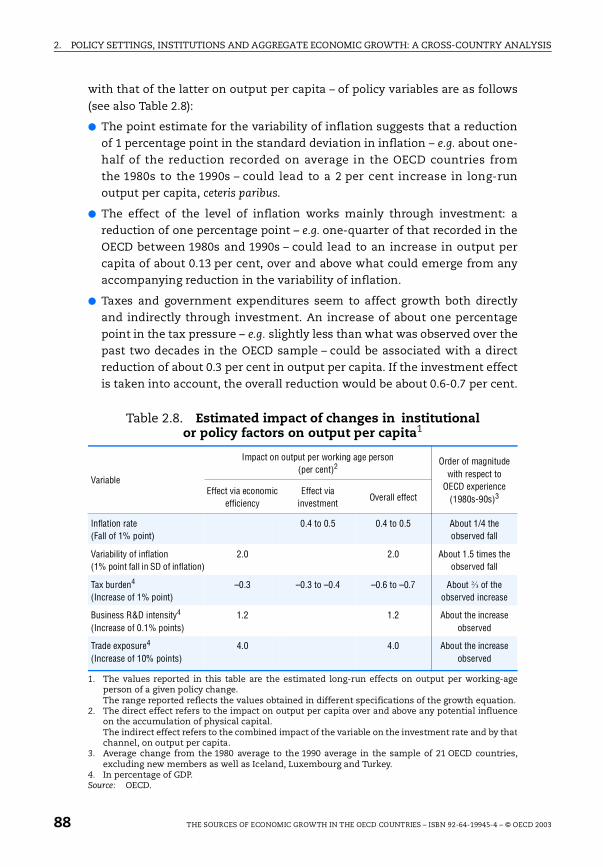
2. POLICY SETTINGS, INSTITUTIONS AND AGGREGATE ECONOMIC GROWTH: A CROSS-COUNTRY ANALYSIS
with that of the latter on output per capita – of policy variables are as follows
(see also Table 2.8):
The point estimate for the variability of inflation suggests that a reductionof 1 percentage point in the standard deviation in inflation – e.g. about one-half of the reduction recorded on average in the OECD countries fromthe 1980s to the 1990s – could lead to a 2 per cent increase in long-runoutput per capita, ceteris paribus.
The effect of the level of inflation works mainly through investment: areduction of one percentage point – e.g. one-quarter of that recorded in theOECD between 1980s and 1990s – could lead to an increase in output percapita of about 0.13 per cent, over and above what could emerge from anyaccompanying reduction in the variability of inflation.
Taxes and government expenditures seem to affect growth both directlyand indirectly through investment. An increase of about one percentagepoint in the tax pressure – e.g. slightly less than what was observed over thepast two decades in the OECD sample – could be associated with a directreduction of about 0.3 per cent in output per capita. If the investment effectis taken into account, the overall reduction would be about 0.6-0.7 per cent.
Table 2.8. Estimated impact of changes in institutional or policy factors on output per capita1
1. The values reported in this table are the estimated long-run effects on output per working-ageperson of a given policy change.The range reported reflects the values obtained in different specifications of the growth equation.
2. The direct effect refers to the impact on output per capita over and above any potential influenceon the accumulation of physical capital.The indirect effect refers to the combined impact of the variable on the investment rate and by thatchannel, on output per capita.
3. Average change from the 1980 average to the 1990 average in the sample of 21 OECD countries,excluding new members as well as Iceland, Luxembourg and Turkey.
4. In percentage of GDP.Source: OECD.
Variable
Impact on output per working age person(per cent)2 Order of magnitude
with respect to OECD experience
(1980s-90s)3Effect via economic efficiency
Effect via investment
Overall effect
Inflation rate(Fall of 1% point)
0.4 to 0.5 0.4 to 0.5 About 1/4 theobserved fall
Variability of inflation(1% point fall in SD of inflation)
2.0 2.0 About 1.5 times the observed fall
Tax burden4
(Increase of 1% point)–0.3 –0.3 to –0.4 –0.6 to –0.7 About ⅔ of the
observed increase
Business R&D intensity4
(Increase of 0.1% points)1.2 1.2 About the increase
observed
Trade exposure4
(Increase of 10% points)4.0 4.0 About the increase
observed
88 THE SOURCES OF ECONOMIC GROWTH IN THE OECD COUNTRIES – ISBN 92-64-19945-4 – © OECD 2003
2. POLICY SETTINGS, INSTITUTIONS AND AGGREGATE ECONOMIC GROWTH: A CROSS-COUNTRY ANALYSIS
A persistent 0.1 percentage point increase in R&D intensity (about 10 per
cent increase with respect to average R&D intensity) would have a long-runeffect of about 1.2 per cent higher output per capita under the“conservative” interpretation of the estimation results. However, in the caseof R&D it is perhaps more appropriate to consider the results as reflecting apermanent effect on growth of GDP per capita (i.e. a fall in R&D intensity isunlikely to reduce the steady-state level of GDP per capita but ratherreduces technical progress). If the R&D coefficient is taken to representgrowth effects, a 0.1 percentage point increase in R&D could boost outputper capita growth by some 0.2 per cent. These estimated effects are large,perhaps unreasonably so, but nevertheless point to significant externalitiesin R&D activities.
Finally, an increase in trade exposure of 10 percentage point – about thechange observed over the past two decades in the OECD sample – could leadto an increase in steady-state output per capita of 4 per cent.
2.4. Concluding remarks
This chapter has investigated empirically the growth contribution ofdifferent forms of investment (physical, human, knowledge) and variouspolicy and institutional settings across OECD countries and over time. In broadterms, the estimated growth regressions explain much of the observed growthpaths across countries and over time. Notably, the results point to a high speedof convergence to the steady-state growth path, compared with previous
estimates based on a larger set of countries and cross-section data. Thisimplies that observed cross-country differences in GDP per capita levels maybe largely the result of differences in long-run equilibrium levels rather thandifferent positions of countries along a similar growth path. Thus, changes inthe determinants of the equilibrium – including the accumulation of physicaland human capital, R&D trade exposure, financial structures andmacroeconomic conditions – can be translated relatively rapidly into changesin living standards.
More specifically, the analysis confirms the importance of investment inphysical and human capital. In the latter case the results also point to potentialexternalities in investment in education, i.e. social returns seem higher thanprivate returns, at least in some countries and periods where education levelswere relatively low. However, these externalities may arise mainly in the caseof compulsory education, insofar as other OECD work indicates that privatereturns may exceed social returns for post-compulsory education.
There is also confirmation that sound macro policy settings are conduciveto higher growth paths. In particular, the reduction in the levels of inflationin most OECD countries could have stimulated the accumulation of physical
THE SOURCES OF ECONOMIC GROWTH IN THE OECD COUNTRIES – ISBN 92-64-19945-4 – © OECD 2003 89
2. POLICY SETTINGS, INSTITUTIONS AND AGGREGATE ECONOMIC GROWTH: A CROSS-COUNTRY ANALYSIS
capital in the private sector and, through this channel, had a positive
bearing on output. Moreover, the reduction in the variability of inflationmay have contributed to a shift in the composition of investment towardsmore risky but also higher return projects.
In addition, the empirical evidence lends some support to the notion thatthe overall size of government in the economy may reach levels that hindergrowth. Although expenditure on health, education and research clearly
sustains living standards in the long term, and social transfers help to meetsocial goals, all have to be financed. The results suggest that for a givenlevel of taxation, higher direct taxes lead to lower output per capita, while,on the expenditure side, government consumption and governmentinvestment tend to have positive effects on output per capita. Governmentinvestment may also influence growth by improving the frameworkconditions (e.g. better infrastructure) in which private agents operate.
Research and development activities undertaken by the business sectorseem to have high social returns, while no clear-cut relationship could beestablished between R&D activities not undertaken by businesses andgrowth. There are, however, possible interactions and internationalspillovers that the regression analysis cannot identify. Moreover, certainpublic R&D (e.g. energy, health and university research) may in the long rungenerate basic knowledge, with possible “technology spillovers”.
Finally, the empirical evidence also confirms the importance of financialmarkets for growth, both by helping to channel resources towards the mostrewarding activities, and in encouraging investment.
Although the factors identified in this chapter appear to be crucial tounderstanding growth patterns across countries and over time, there are anumber of additional determinants that could not be directly analysed. Inparticular, in the current period, characterised by a process of adaptation toinformation and communication technologies, a number of other policy andinstitutional factors are also likely to play a key role, by influencing the abilityof markets to adapt to the new technologies. The latter requires reallocatingresources to new activities, re-shaping existing firms and discovering newbusiness opportunities. The subsequent chapters will look at theseinstitutional and policy factors exploring their impact on industry andindividual firms’ performance.
Notes
1. This chapter draws heavily from Bassanini, Hemmings and Scarpetta (2001).
2. This extreme view may not hold, even in neo-classical models, if one assumesthat policy, by influencing the allocation of resources across individuals, mayaffect saving behaviour.
90 THE SOURCES OF ECONOMIC GROWTH IN THE OECD COUNTRIES – ISBN 92-64-19945-4 – © OECD 2003
2. POLICY SETTINGS, INSTITUTIONS AND AGGREGATE ECONOMIC GROWTH: A CROSS-COUNTRY ANALYSIS
3. For example, new-growth models that incorporate a knowledge-producing sectorcan be interpreted as incorporating the role that research universities may play ingrowth. An early example of this type of model was by Uzawa (1965), laterexamples by Lucas (1988), Romer (1990), Grossman and Helpman (1991) andAghion and Howitt (1998).
4. OECD (2000a) provides more details on recent trends in R&D intensity. Inparticular, the decline in government spending in R&D has been affected by thereduction in the military R&D budget in the aftermath of the end of the cold war.Moreover, government spending declined in the early 1990s as a result of theefforts to reduce fiscal imbalances.
5. See Temple (1998) for a comprehensive discussion of theories linking inflationwith growth.
6. For instance, the tax structure usually includes nominally-denominatedallowances, so that as inflation rises, tax allowances (credits) decline and theeffective cost of investment rises (Jones and Manuelli, 1993). Moreover, if money isrequired to buy capital goods, the effective cost of capital increases with theinflation rate (Stockman, 1981 ; De Gregorio, 1993).
7. Mundell (1963) ; Tobin (1965).
8. See Ball and Cecchetti (1990) for a review.
9. Barro (1976, 1980). Several studies show that the variability of prices across goodsand the variability of prices of the same goods across stores increases with inflation(see Lach and Tsiddon, 1992, for a survey).
10. See Bernanke (1983) Pindyck (1991), and Ramey and Ramey (1995). However, not alllinks between output volatility and growth may be negative. For instance, somehave argued that there may be a choice between high-variance, high-expected-returns technologies and low-variance, low-expected-returns technologies(e.g. Black, 1987). Lower output volatility would tend to be associated with loweroutput growth. Moreover, one should keep in mind that cross-country differencesin the volatility of output may, to some extent, reflect differences in the “size” ofeconomies. Greater diversity of activities in larger economies implies that sector-specific shocks carry less weight in aggregate outcomes. In addition, “large”economies are typically less exposed to external shocks as trade balances arerelatively small compared with smaller economies.
11. These two countries have experienced very large and opposite changes in theirvariability of inflation from the 1980s to the 1990s, while at the same timeimproving their growth performance.
12. For example, long-run data often show that government expenditure as a share ofGDP tends to rise with living standards (Wagner’s law), reflecting income-elasticdemand for key government services (health, education and law and order).Kolluri et al. (2000) find strong support for Wagner’s law operating in OECDcountries, based on regressions linking total government expenditure with GDP.
13. See amongst others, Barro (1990); Barro and Sala-i-Martin (1995); Mendoza et al. (1997).
14. Unlike non-distortionary taxes, distortionary taxes affect the economic choices ofhouseholds and firms, notably with respect to the level and composition of their(human and physical) capital investment. By contrast, non-distortionary taxes aremore neutral. Non-distortionary taxes mainly relate to taxation on domesticgoods and services, while distortionary taxes include taxation on income andprofits, taxation on payroll and manpower. Some simulations made by Jorgenson
THE SOURCES OF ECONOMIC GROWTH IN THE OECD COUNTRIES – ISBN 92-64-19945-4 – © OECD 2003 91
2. POLICY SETTINGS, INSTITUTIONS AND AGGREGATE ECONOMIC GROWTH: A CROSS-COUNTRY ANALYSIS
and Yun (1986, 1990) show that a shift from direct to indirect taxation could leadto significant output gains in the United States.
15. Transfer programmes are often taken as examples of the second group (see e.g.Hubbard et al., 1995; Leonard and Audenrode, 1993). However, redistributionaltransfers may buy poor people out of disruptive activities, with potentiallypositive effect on output growth (Sala-i-Martin, 1997; Phelps, 2000).
16. One limitation of the stock market capitalisation indicator is that it does notcapture the development of the banking system, the role of debt securities, orother parts of the equity market (not-listed equity). Moreover, it measures themarket value of existing listed companies rather than the amount of funds raisedin the equity market in any particular year.
17. For example, if a variable has a positive bearing on output independently of itspositive impact on investment, its estimated coefficient in a growth regressionthat includes, on the right-hand side, the investment rate, will under-represent itstotal impact on output. Alternatively, if the policy variable has a positiveindependent effect on output growth but a negative effect on investment, theestimated coefficient in the growth regression will exaggerate the effect of thepolicy variable on growth.
18. Where data for a large number of countries was available, growth regressions havetypically taken averages over long time periods (e.g. 20 years). Other studies havetaken averages over 5-year periods (see e.g. Islam, 1995; Caselli et al., 1996). Theuse of time averages raises two possible problems: it implies a potential loss ofinformation; and, more importantly, in cases of un-synchronised business cycles.,it does not purge the data from country-specific cyclical influences.
19. This concerns, for example, one-sector models of endogenous growth in whichcapital is not characterised by diminishing returns (see e.g. Romer, 1986;Rebelo, 1991).
20. This concerns models of endogenous growth, which explicitly consider differenttypes of capital goods (e.g. physical and human), each characterised by its ownaccumulation process (e.g. investment and education). See Uzawa (1965); Lucas(1988); Barro and Sala-i-Martin (1995).
21. Estimates of the speed of convergence to steady-state output vary in the literature:while most studies estimated values around 2-3 per cent per year (Mankiw, et al.,1992; Barro and Sala-i-Martin, 1995) – which implies that an economy spendsabout 20-30 years to cover half of the distance between its initial conditions andits steady state – a few have found values of 10 per cent or more for the OECDcountries (e.g. Caselli et al., 1996), which imply less than 9 years to cover half of thedistance.
22. The country sample include: Australia, Austria, Belgium, Canada, Denmark,Finland, France, Germany (western), Greece, Ireland, Italy, Japan, Netherlands,New Zealand, Norway, Portugal, Spain, Sweden, Switzerland, the United Kingdomand the United States.
23. This is obtained from the long-run coefficient (the partial long-run elasticity) andthe implied variation from a one percentage point change in the cross-countryaverage investment share.
24. Using a similar proxy, de la Fuente and Doménech (2000) also found a stronglysignificant coefficient for human capital in level and growth equations, whichconfirms the important role of data quality.
92 THE SOURCES OF ECONOMIC GROWTH IN THE OECD COUNTRIES – ISBN 92-64-19945-4 – © OECD 2003
2. POLICY SETTINGS, INSTITUTIONS AND AGGREGATE ECONOMIC GROWTH: A CROSS-COUNTRY ANALYSIS
25. However, these results may also be driven by distortions (e.g. excessive taxation orwage compression) that discourage investment in human capital by individuals.
26. It should be stressed that these conclusions do not depend on a particularspecification of the growth regression. They are indeed confirmed by a sensitivityanalysis presented in Bassanini and Scarpetta (2001).
27. Each policy-augmented specification was estimated with and without the tradeexposure variable to test for the sensitivity of coefficients. As discussed inBassanini and Scarpetta (2001), the coefficient on trade exposure is alwayssignificant and the equations reported here include this variable. These results areconsistent with, amongst others, Miller and Russek (1997) who focused on OECDcountries in their empirical analyses.
28. The overall measure of tax and non-tax revenue can be used only for a sub-sampleof 18 OECD countries, due to data availability.
29. The coefficient on government consumption becomes negative once the financingvariables are excluded because, in this case, government consumption acts as aproxy for the "size" of government intervention.
30. By contrast, government investment becomes insignificant as soon as the modelis extended and is dropped in the final specification on the right-hand side of theTable.
31. In particular, the analysis is restricted to 14-17 countries (depending on thespecification) and the period 1981-98 (and for some countries the period isshorter). The shorter time-series significantly restrict the number of variables thatcould be considered in the regressions. These include, in addition to the R&Dvariables, the basic controls and trade exposure, whenever possible. It should bestressed that the coefficients on both physical and human capital maintain thesign and statistical significance they had in the regressions estimated over thelarger sample, although convergence is faster. This latter result is not driven by thesmall country sample but rather by the shorter time period over which the modelis estimated (see Bassanini and Scarpetta, 2001)
32. See Fagerberg (1994); and Englander and Gurney (1994).
33. Park (1995) also found private-sector R&D to be more important than public R&Din OECD-based growth regressions.
34. These possible interactions between R&D and international trade have beenemphasised by several other studies. For instance, Coe and Helpman (1995) findsignificant interaction between import propensities and the ability to benefit fromforeign R&D: i.e. for a given level of R&D performed abroad, countries with higherimport propensity have higher productivity growth. Moreover, small countriesbenefit more from R&D performed abroad than from domestic R&D. Sachs andWarner (1995) claim trade openness as being an important constraint toconvergence for many developing countries. At the same time, Ben-David andKimhi (2000), using aggregate data on trade between (mainly) OECD countries, findevidence to support the idea that increasing trade between pairs of countries isassociated with an increased rate of convergence.
35. Lichtenberg (1988) finds that non-competitive R&D procurement tends to crowdout private R&D investment, while competitive procurement stimulates it. SeeDavid et al. (1999) for a survey. By contrast, Guellec and Van Pottelsberghe (1997,2001) support the complementarity hypothesis.
THE SOURCES OF ECONOMIC GROWTH IN THE OECD COUNTRIES – ISBN 92-64-19945-4 – © OECD 2003 93

2. POLICY SETTINGS, INSTITUTIONS AND AGGREGATE ECONOMIC GROWTH: A CROSS-COUNTRY ANALYSIS
36. Given the short time period that can be used in this sample, lagging the R&Dvariable would have induced an excessive loss of degrees of freedom.
37. Following experimentation with three control variables, lagged output per capita,human capital and lagged trade exposure, the preferred specification includesonly a control for trade exposure (see Bassanini and Scarpetta, 2001).
38. However, data limitations constrained the number of variables that could beincluded alongside the indicator of stock market capitalisation. Moreover, theinterpretation of the causality link between stock market capitalisation andinvestment may be problematic: the former is driven by changes in valuation oflisted companies which in turn could be driven by factors also influencinginvestment.
94 THE SOURCES OF ECONOMIC GROWTH IN THE OECD COUNTRIES – ISBN 92-64-19945-4 – © OECD 2003

ISBN 92-64-19945-4
The Sources of Economic Growth in the OECD Countries© OECD 2003
Chapter 3
What Drives Productivity Growth at the Industry Level?
Abstract. This chapter1 extends the analysis of how policy influencesgrowth by exploring industry-level data. In particular, it assesses howdifferent policy and institutional settings in both product and labourmarkets affect productivity and innovation activity. Aggregateproductivity patterns are largely the result of within-industryperformance in the OECD countries, and the latter is negatively affectedby strict product market regulations, especially if there is a significanttechnology gap with the technology leader. There is also evidence of anindirect negative effect of strict product market regulations onproductivity via their impact on innovation activity. Likewise, by raisinglabour adjustment costs, strict employment protection legislation tends tohinder productivity, unless these higher costs are offset by lower wagesand/or more internal training. However, strict employment protectionlegislation does not affect innovation activity, but rather tends to tiltsectoral specialisation towards industries where technologicalenhancement can be accommodated with internal training.
THE SOURCES OF ECONOMIC GROWTH IN THE OECD COUNTRIES – ISBN 92-64-19945-4 – © OECD 2003 95
3. WHAT DRIVES PRODUCTIVITY GROWTH AT THE INDUSTRY LEVEL?
Introduction
Assessing the role of policy and institutions for long-term growth cannotbe limited to aggregate analysis. It also requires exploration of the role playedby within-industry performance and reallocation of resources acrossindustries and firms. Indeed, the macro analysis may fail to capture the effectsof specific policies – such as product market regulations and traderestrictions – on industry performance. Likewise, differences in growthpatterns at the industry level may also point to variations in the extent towhich countries are benefiting from broader economic changes, or from the
potential offered by new technologies. For example, as discussed in Chapter 1,technological change has enabled rapid productivity growth in the ICT-producing industry and, most recently, in ICT-using industries, but there areconsiderable variations in the degree to which countries have benefited fromsuch potential. The remainder of the book is devoted to the exploration ofthese aspects of growth, by using industry and firm-level data.
The purpose of this chapter is twofold. It first reviews the role played bywithin-industry growth and reallocation across industries in the growthprocess (Section 3.1). It finds that most of the observed aggregate productivitygrowth is due to within-industry performance, with only a minor role playedby the reallocation of resources from less to more productive industries.However, there is also evidence that certain industries – mostly related toICT – have made a particularly strong contribution to overall productivitygrowth in some countries. This finding, in turn, raises the more generalquestion as to why some countries have more than others enjoyedproductivity gains associated with innovation and adoption of newtechnologies. The chapter addresses this question analytically, by assessing
the role of policy and institutional settings – in particular product and labourmarket regulations – in driving productivity growth (Section 3.2). Thiscomplements the analysis presented in Chapter 2 that focused on the role ofaggregate framework conditions for productivity and growth.
3.1. Within-industry growth and reallocation of resources across industries
The analysis of sectoral performance and its contribution to aggregategrowth patterns is organised as follows. The contribution of structural shiftsacross broad sectors of the economy to overall productivity patterns is first
96 THE SOURCES OF ECONOMIC GROWTH IN THE OECD COUNTRIES – ISBN 92-64-19945-4 – © OECD 2003

3. WHAT DRIVES PRODUCTIVITY GROWTH AT THE INDUSTRY LEVEL?
assessed. Since most of aggregate productivity growth seems to be due to
within industry patterns, the section then focuses on the sources ofproductivity growth at the sectoral level.
Structural changes and labour productivity growth
Historically, structural shifts were an important factor behindproductivity growth as resources moved from a low-productive agricultural
sector to a more productive manufacturing sector. More recently, however,evidence from aggregate data seems to suggest that a large contribution tooverall productivity growth patterns comes from productivity changes withinindustries, rather than as a result of significant shifts of employment acrossindustries (Van Ark, 1996). For the purpose of international comparison,Figure 3.1 presents a decomposition of labour productivity growth in thebusiness sector into three elements:2
An “intra-sectoral effect”, measuring productivity growth within industries.
A “net-shift effect”, measuring the impact on productivity of the shift inemployment between industries.
And a residual third effect, the “interaction effect”. This effect is positivewhen sectors with rapid productivity growth also increase their industryemployment share, or when industries with falling relative productivitydecline in size. It is negative when industries with growing relativeproductivity decline in size or when industries with falling productivitygrow in size.
Bearing in mind the limits of a decomposition based on rather broadindustries, the results of these calculations show that the intra-industry effectis the most important contributor to productivity growth in the non-farmbusiness sector (Figure 3.1). In a few countries the net-shift effect also makesan important contribution, due notably to the increased size of the businessservices sector, but its impact seems to fade out during the 1990s. Theinteraction effect tends to be negative for most countries.3 These results are inline with those obtained when looking at manufacturing only (Figure 3.1):
employment shifts across manufacturing industries played a very modest rolein most countries.
The evidence that productivity growth is more than ever a matter ofperformance improvement within industries is perhaps not surprising for thecountries examined in Figure 3.1, as around 70 per cent of value-added inthese countries is already in services. However, other OECD economies,
including Ireland and Japan, as well as some low-income countries, have amuch smaller business service sector, suggesting that there may be furtherscope for structural change. In addition, there is likely to be scope for further
THE SOURCES OF ECONOMIC GROWTH IN THE OECD COUNTRIES – ISBN 92-64-19945-4 – © OECD 2003 97
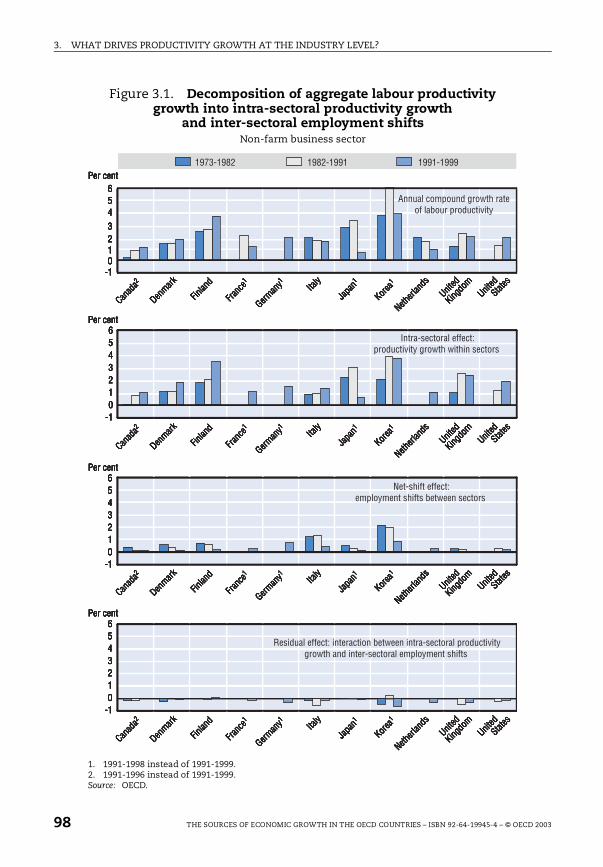
3. WHAT DRIVES PRODUCTIVITY GROWTH AT THE INDUSTRY LEVEL?
Figure 3.1. Decomposition of aggregate labour productivity growth into intra-sectoral productivity growth
and inter-sectoral employment shiftsNon-farm business sector
1. 1991-1998 instead of 1991-1999.2. 1991-1996 instead of 1991-1999.Source: OECD.
1973-1982 1982-1991 1991-1999
Annual compound growth rateof labour productivity
Per cent
Per cent
Per cent
Canad
a2
Denmark
Finlan
d
Franc
e1
German
y1 Italy
Japa
n1
Korea1
Netherl
ands
United
Kingdo
mUnit
edStat
es
Canad
a2
Denmark
Finlan
d
Franc
e1
German
y1 Italy
Japa
n1
Korea1
Netherl
ands
United
Kingdo
mUnit
edStat
es
Canad
a2
Denmark
Finlan
d
Franc
e1
German
y1 Italy
Japa
n1
Korea1
Netherl
ands
United
Kingdo
mUnit
edStat
es
Canad
a2
Denmark
Finlan
d
Franc
e1
German
y1 Italy
Japa
n1
Korea1
Netherl
ands
United
Kingdo
mUnit
edStat
es
Intra-sectoral effect:productivity growth within sectors
Residual effect: interaction between intra-sectoral productivitygrowth and inter-sectoral employment shifts
-10123456
Per cent
Net-shift effect:employment shifts between sectors
-10123456
-10123456
-10123456
98 THE SOURCES OF ECONOMIC GROWTH IN THE OECD COUNTRIES – ISBN 92-64-19945-4 – © OECD 2003
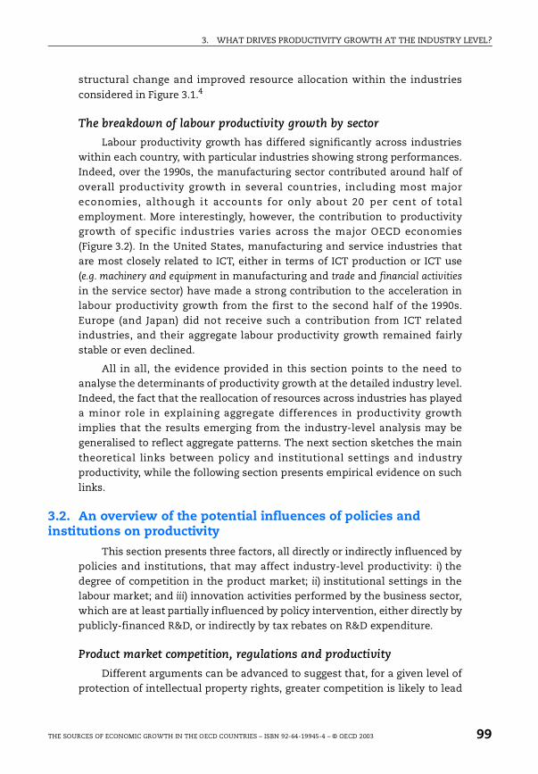
3. WHAT DRIVES PRODUCTIVITY GROWTH AT THE INDUSTRY LEVEL?
structural change and improved resource allocation within the industries
considered in Figure 3.1.4
The breakdown of labour productivity growth by sector
Labour productivity growth has differed significantly across industrieswithin each country, with particular industries showing strong performances.Indeed, over the 1990s, the manufacturing sector contributed around half of
overall productivity growth in several countries, including most majoreconomies, although it accounts for only about 20 per cent of totalemployment. More interestingly, however, the contribution to productivitygrowth of specific industries varies across the major OECD economies(Figure 3.2). In the United States, manufacturing and service industries thatare most closely related to ICT, either in terms of ICT production or ICT use(e.g. machinery and equipment in manufacturing and trade and financial activities
in the service sector) have made a strong contribution to the acceleration inlabour productivity growth from the first to the second half of the 1990s.Europe (and Japan) did not receive such a contribution from ICT relatedindustries, and their aggregate labour productivity growth remained fairlystable or even declined.
All in all, the evidence provided in this section points to the need toanalyse the determinants of productivity growth at the detailed industry level.Indeed, the fact that the reallocation of resources across industries has playeda minor role in explaining aggregate differences in productivity growthimplies that the results emerging from the industry-level analysis may begeneralised to reflect aggregate patterns. The next section sketches the main
theoretical links between policy and institutional settings and industryproductivity, while the following section presents empirical evidence on suchlinks.
3.2. An overview of the potential influences of policies and institutions on productivity
This section presents three factors, all directly or indirectly influenced bypolicies and institutions, that may affect industry-level productivity: i) thedegree of competition in the product market; ii) institutional settings in thelabour market; and iii) innovation activities performed by the business sector,which are at least partially influenced by policy intervention, either directly bypublicly-financed R&D, or indirectly by tax rebates on R&D expenditure.
Product market competition, regulations and productivity
Different arguments can be advanced to suggest that, for a given level ofprotection of intellectual property rights, greater competition is likely to lead
THE SOURCES OF ECONOMIC GROWTH IN THE OECD COUNTRIES – ISBN 92-64-19945-4 – © OECD 2003 99
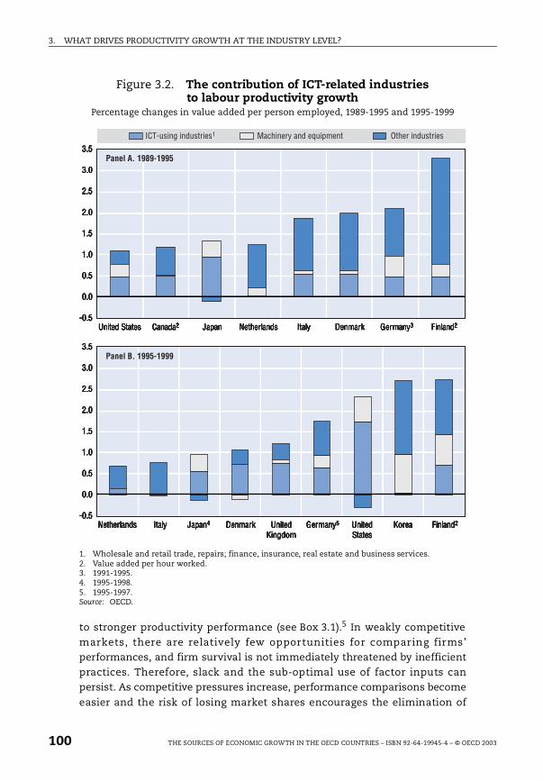
3. WHAT DRIVES PRODUCTIVITY GROWTH AT THE INDUSTRY LEVEL?
to stronger productivity performance (see Box 3.1).5 In weakly competitivemarkets, there are relatively few opportunities for comparing firms’performances, and firm survival is not immediately threatened by inefficientpractices. Therefore, slack and the sub-optimal use of factor inputs canpersist. As competitive pressures increase, performance comparisons become
easier and the risk of losing market shares encourages the elimination of
Figure 3.2. The contribution of ICT-related industries to labour productivity growth
Percentage changes in value added per person employed, 1989-1995 and 1995-1999
1. Wholesale and retail trade, repairs; finance, insurance, real estate and business services.2. Value added per hour worked.3. 1991-1995.4. 1995-1998.5. 1995-1997.Source: OECD.
3.0
3.5
2.0
2.5
1.0
1.5
0.0
-0.5
0.5
3.0
3.5
2.0
2.5
1.0
1.5
0.0
-0.5
0.5
United States Canada2 Japan Netherlands Italy Denmark Germany3 Finland2
Panel A. 1989-1995
UnitedStates
UnitedKingdom
KoreaJapan4Netherlands Italy Denmark Germany5 Finland2
Panel B. 1995-1999
ICT-using industries1 Machinery and equipment Other industries
3.0
3.5
2.0
2.5
1.0
1.5
0.0
-0.5
0.5
3.0
3.5
2.0
2.5
1.0
1.5
0.0
-0.5
0.5
United States Canada2 Japan Netherlands Italy Denmark Germany3 Finland2
Panel A. 1989-1995
UnitedStates
UnitedKingdom
KoreaJapan4Netherlands Italy Denmark Germany5 Finland2
Panel B. 1995-1999
ICT-using industries1 Machinery and equipment Other industries
100 THE SOURCES OF ECONOMIC GROWTH IN THE OECD COUNTRIES – ISBN 92-64-19945-4 – © OECD 2003

3. WHAT DRIVES PRODUCTIVITY GROWTH AT THE INDUSTRY LEVEL?
Box 3.1. The theoretical links between product market competition and productivity
Textbook theory suggests that competition in the product marketbrings about allocative efficiency gains by forcing prices to converge tomarginal costs. In addition to such static gains, a variety of theoreticalanalyses based on information asymmetry between managers andowners have indicated potential gains from “dynamic efficiency”. Thesedynamic gains are likely to emerge because firms will continue to
improve their performance in ways they would not if competitivepressures were weak (Winston, 1993).
Theoretical models focusing on dynamic efficiency generally originatefrom the idea that monopoly rents are often captured by managers (andpossibly workers) in the form of managerial “slack” or reduced workeffort. In this context, at least three different channels can be identified,
through which product market competition would discipline firms intoefficient operation (Nickell et al., 1997). First, competition creates greateropportunities for comparing performance, making it easier for theowners or the market to monitor managers (Lazear and Rosen, 1981;Nalebuff and Stiglitz, 1983). Second, cost-reducing improvements inproductivity could generate higher revenue and profit in a morecompetitive environment, where price elasticity of demand tends to behigher. Third, since more competition is likely to raise the likelihood ofbankruptcy, managers may work harder to avoid this outcome (Aghionand Howitt, 1998). In addition, if product market rents are partly sharedwith workers in the form of higher wages or reduced effort, thencompetition probably influences workers’ behaviour too (Haskel and
Sanchis, 1995).
It should be stressed that theoretical predictions of the effects ofgreater competition on incentives are often “subtle and ambiguous”(Vickers, 1995). For example, though models using explicit incentivesunder information asymmetry do not lead to clear-cut implications(see e.g. Holmström, 1982), intertemporal models using implicit
(i.e. market-based) rewards suggest a positive link between competitionand managerial effort if productivity shocks are more correlated acrosscompetitors than managerial abilities (Meyer and Vickers, 1997). Butcompetition could, on the contrary, lead to more slack if managers arehighly responsive to monetary incentives (Scharfstein, 1988). Similarly,while higher demand elasticity under competition increases the relativerewards from cost reduction, larger scale operations for a monopolist
THE SOURCES OF ECONOMIC GROWTH IN THE OECD COUNTRIES – ISBN 92-64-19945-4 – © OECD 2003 101
3. WHAT DRIVES PRODUCTIVITY GROWTH AT THE INDUSTRY LEVEL?
slack. In parallel, the need to meet the cost efficiency of competing firmsprovides a powerful motivation for adjusting technology and workorganisation to best practice.
However, the empirical evidence supporting these arguments is still fairlylimited,6 partly due to the difficulty of measuring competitive pressures.Traditional indicators of product market conditions used in most studies, suchas mark-ups, industry concentration indexes7 or market shares,8 cannot betreated as exogenous determinants of economic outcomes. For example, highproductivity firms may gain market shares and enjoy innovation rents in astill highly competitive environment. More broadly, recent research showsthat these indicators are not unequivocally related to product market
competition.9 Furthermore, they fail to provide a direct link to policy orregulation, making it difficult to draw policy conclusions.
Box 3.1. The theoretical links between product market competition and productivity (cont.)
tend to increase the absolute reward from a similar cost reduction. All inall, depending on the setting of the model, competition is shown toimprove efficiency in many, but not all, circumstances.
The effect of competition on productivity through innovative activityhas also been extensively analysed. In the basic Schumpeterianapproach, innovation and growth decline with competition because themonopoly rents from innovations tend to be dissipated more quicklywhen there is greater competition, thereby lowering the expectedreturns from innovations. However, the empirical evidence tends toshow an opposite, i.e. positive, relationship. In order to reconcile theorywith this empirical evidence, Aghion and Howitt (1998) have extendedthe basic Schumpeterian model to offer several cases where competition
can be conducive to greater innovation. First, in a rapidly changingtechnological environment, there might be a Darwinian effect, wherebyintensified competition forces managers to speed up the adoption ofnew technologies in order to avoid bankruptcy. Even if technologicalprogress is more gradual, i.e. when firms are engaged in step-by-stepinnovative activities, greater competition may induce “neck-and-neck”
firms to invest more in R&D in order to acquire a lead over their rivals(see also Aghion et al., 2001). Finally, insofar as increased competitionincreases the mobility of skilled workers to newer lines, it may stimulateoverall growth in the presence of learning by doing (mobility effect).
102 THE SOURCES OF ECONOMIC GROWTH IN THE OECD COUNTRIES – ISBN 92-64-19945-4 – © OECD 2003
3. WHAT DRIVES PRODUCTIVITY GROWTH AT THE INDUSTRY LEVEL?
The empirical analysis presented in this chapter is, therefore, based on
some of the potential policy determinants of competition rather than on directmeasures of it. Specifically, the focus is on indicators of the stringency ofproduct market regulations. The main effect of pro-competitive productmarket regulations is to strengthen the incentives to improve productivity andadopt new technologies.
Labour market institutions and productivity
Although labour market regulations are primarily designed to ensuresocially desirable outcomes,10 some of them can affect the costs ofimplementing measures aimed at improving efficiency. For example,restrictions on hiring and firing are often found to reduce incentives forinternal efficiency by hindering the labour adjustments generally associatedwith such efforts.11 At the same time, bargaining systems may affect the wayrents associated with process and product innovation are appropriated byfirms and workers. Systems that favour the sharing of innovation rents withworkers (for instance by increasing the bargaining power of insiders or tyingnegotiations to enterprise performance) may inhibit innovative activity byreducing the expected returns from innovations; conversely, systems that
favour the appropriation of rents by firms, for instance by co-ordinatingindividual bargaining processes at the industry or nation-wide level, andcompressing wage structures so that wages are lower for skilled workers, mayincrease incentives to innovate (Teulings and Hartog, 1998).
Innovation, R&D and productivity
The direct effects of policy and institutions on MFP are likely to becombined with indirect effects stemming from their influence on R&D activity.First, R&D can boost productivity, either directly via the stream of innovationit produces,12 or more indirectly via the adoption of existing technologiesdeveloped elsewhere.13 This latter channel implies that the further a countryis away from the technology frontier, the greater the benefits from R&D, bystimulating domestic and international knowledge spillovers. Second, there isevidence that interaction between strict EPL and certain industrial relationsregimes, or certain aspects of product market regulations, have a detrimentaleffect on R&D activity.14
3.3. Empirical analysis
Direct determinants of productivity
The empirical analysis presented in this section focuses on industry-levelmulti-factor productivity. The latter offers a better proxy for the level ofeconomic efficiency than labour productivity measures, especially in an
THE SOURCES OF ECONOMIC GROWTH IN THE OECD COUNTRIES – ISBN 92-64-19945-4 – © OECD 2003 103
3. WHAT DRIVES PRODUCTIVITY GROWTH AT THE INDUSTRY LEVEL?
international comparison when differences in labour productivity may reflect
differences in the labour intensity rather than differences in productionefficiency (see Chapter 1). The productivity equation is derived from atheoretical framework in which MFP depends on country/industry specificfactors, and on a catch-up term that measures the distance from thetechnological frontier (i.e. the most productive country) in each industry (seeBox 3.2, and Annex 3 for further details). This framework permits testing forthe direct effect of institutions and regulations on efficiency,15 as well as forthe indirect influences of these factors via the process of technologytransfer.16
The empirical analysis covers 23 industries in manufacturing andbusiness services in 18 OECD countries over the period 1984-1998.17 Thecatch-up term, representing the distance from the technological frontier, isproxied by the difference between the MFP level in a particular industry andthe highest level amongst countries for that industry. Albeit crude, thismeasure broadly confirms expectations about which countries and regionstend to be at the forefront of technology in certain fields (see Scarpetta andTressel 2002 for details): the United States, Canada and Japan were often at thefrontier in most industries over the period considered. However, if differences
in hours worked are taken into account (as in the preferred measure of MFP),then a number of European countries were also close to the technologyfrontier. The comparison of MFP levels also suggests that in only a few casesdoes the identity of the frontier remain constant, which implies that somecountries “leapfrogged” others in terms of technology leadership in mostindustries. However, what matters for productivity growth is the distancefrom the technological frontier – which captures the potential for technologytransfer – rather than the identity of the frontier itself.
Table 3.1 presents the main results of the MFP regressions.18 Thetechnology-gap term (RMFP) is found to have a significant negative effect onMFP growth, suggesting that within each industry (with the exception of high-tech manufacturing industries, see below), countries that are further behindthe frontier experience higher rates of productivity growth. However,confirming some previous results (e.g. Bernard and Jones, 1996a, b), there isevidence of a more rapid technological catch-up in service industries than inmanufacturing. This is true both in terms of short-term technological “passthrough” (i.e. the coefficient of MFP growth in the leader country, ∆MFPleader),
which is statistically insignificant for manufacturing industries, as well asover the longer run as shown by the higher coefficient on the technology-gapterm for services. This is consistent with the view that convergence isrelatively easier when technology is more standardised, as in many servicesectors, than in cases where it is more diversified, as in many manufacturingindustries.
104 THE SOURCES OF ECONOMIC GROWTH IN THE OECD COUNTRIES – ISBN 92-64-19945-4 – © OECD 2003
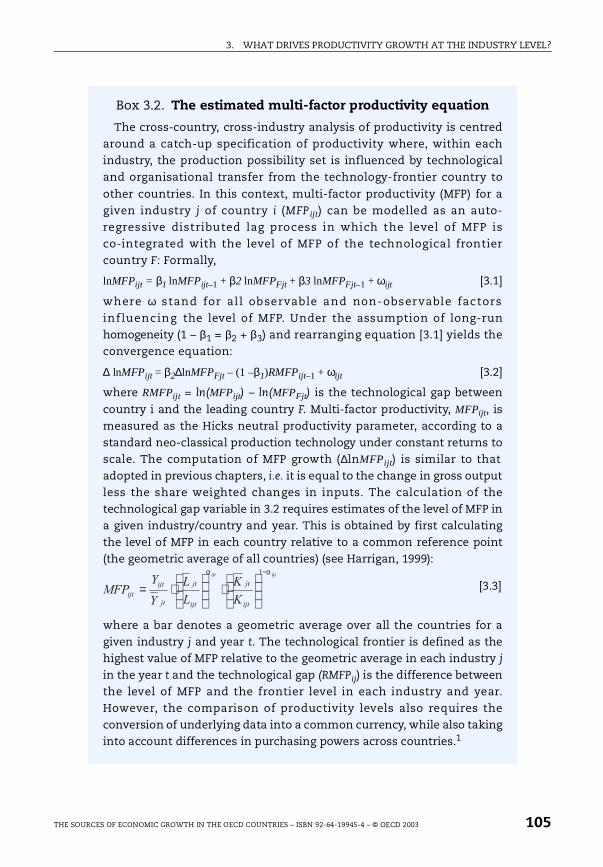
3. WHAT DRIVES PRODUCTIVITY GROWTH AT THE INDUSTRY LEVEL?
Box 3.2. The estimated multi-factor productivity equation
The cross-country, cross-industry analysis of productivity is centredaround a catch-up specification of productivity where, within eachindustry, the production possibility set is influenced by technologicaland organisational transfer from the technology-frontier country to
other countries. In this context, multi-factor productivity (MFP) for agiven industry j of country i (MFP ijt) can be modelled as an auto-regressive distributed lag process in which the level of MFP isco-integrated with the level of MFP of the technological frontiercountry F: Formally,
lnMFPijt = β1 lnMFPijt–1 + β2 lnMFPFjt + β3 lnMFPFjt–1 + ωijt [3.1]
where ω stand for al l observable and non-observable factorsinf luencing the level of MFP. Under the assumption of long-runhomogeneity (1 – β1 = β2 + β3) and rearranging equation [3.1] yields theconvergence equation:
∆ lnMFPijt = β2∆lnMFPFjt – (1 –β1)RMFPijt–1 + ωijt [3.2]
where RMFPijt = ln(MFPijt) – ln(MFPFjt) is the technological gap between
country i and the leading country F. Multi-factor productivity, MFPijt, ismeasured as the Hicks neutral productivity parameter, according to astandard neo-classical production technology under constant returns toscale. The computation of MFP growth (∆lnMFPijt) is similar to thatadopted in previous chapters, i.e. it is equal to the change in gross outputless the share weighted changes in inputs. The calculation of thetechnological gap variable in 3.2 requires estimates of the level of MFP ina given industry/country and year. This is obtained by first calculatingthe level of MFP in each country relative to a common reference point(the geometric average of all countries) (see Harrigan, 1999):
where a bar denotes a geometric average over all the countries for agiven industry j and year t. The technological frontier is defined as thehighest value of MFP relative to the geometric average in each industry jin the year t and the technological gap (RMFPij) is the difference betweenthe level of MFP and the frontier level in each industry and year.However, the comparison of productivity levels also requires theconversion of underlying data into a common currency, while also takinginto account differences in purchasing powers across countries.1
ijt1 αα −
⋅
⋅=
ijt
jt
ijt
jt
jt
ijt
ijtK
K
L
L
Y
YMFP
ijt
[3.3]
THE SOURCES OF ECONOMIC GROWTH IN THE OECD COUNTRIES – ISBN 92-64-19945-4 – © OECD 2003 105

3. WHAT DRIVES PRODUCTIVITY GROWTH AT THE INDUSTRY LEVEL?
The policy-augmented productivity regressions clearly show a stronginfluence of product and labour market regulations on industry productivity(see Box 3.3 for details on the regulatory indicators). In particular, there is anegative direct effect of product market regulations on productivity,whichever indicator is considered.19 However, if the interaction of regulationwith the technology gap is also considered (variable PMR*RMFPijt-1 in equations
E to H), the results indicate a statistically more significant indirect effect ofregulations on productivity via a slower adoption of existing technologies:strict regulations seem to have a particular detrimental effect on productivitythe further the country is from the technology frontier, possibly because theyreduce the scope for knowledge spillovers.
The analysis is also extended to consider the industrial relationsregimes20 and summary indicators of employment protection legislation thatproxy the cost of labour adjustment. The results suggest that differentindustrial relations regimes do not matter per se (the variables related tocorporatism (the bargaining system) are not significant in equation L andonwards), but they may, nevertheless, negatively affect productivity via theirinteractions with EPL. Indeed, there is evidence that the negative impact ofEPL on productivity (shown by equation K) only applies to countries with anintermediate degree of centralisation/co-ordination, i.e. where sectoral wagebargaining is predominant without co-ordination. By contrast, EPL is not
Box 3.2. The estimated multifactor productivity equation (cont.)
The technology gap variable relates to the aggregate convergenceliterature discussed in Chapter 2. Specifically, it allows tests of whetherconvergence – generally found in macro analyses – is driven byspecialisation between industries and/or convergence within industries
(see Dollar and Wolff, 1988, 1993). The residual in equation [3.2] ismodelled as follows:
where (Vijt) is a vector of covariates (e.g. product and market labourregulations) affecting the level of MFP; fi , gj, and dt are respectivelycountry, industry and year fixed effects. ε is an iid shock. Moreover,
equation 3.2 can be solved for steady-state MFP in country i relative tothe frontier in industry j, which gives insights on the effects of thesecountry and/or country-industry-specific factors on the steady-statelevel of MFP.
1. The analysis in this paper uses industry-specific expenditure PPPs, but the sensitivityanalysis also tests the robustness of results by using aggregate PPPs.
ijttji
k
kijtkijt dgfV εγω ++++= ∑ −1 [3.4]
106 THE SOURCES OF ECONOMIC GROWTH IN THE OECD COUNTRIES – ISBN 92-64-19945-4 – © OECD 2003
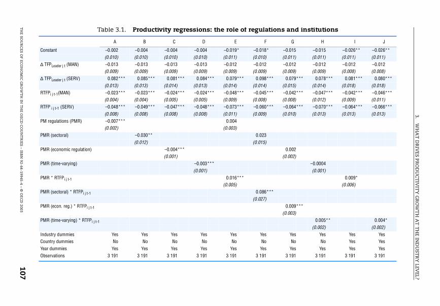
3.W
HA
T D
RIV
ES PRO
DU
CT
IVIT
Y G
RO
WT
H A
T T
HE IN
DU
STR
Y LEV
EL?
TH
E SOU
RC
ES OF EC
ON
OM
IC G
RO
WT
H IN
TH
E OEC
D C
OU
NT
RIES
– ISB
N 92-64-19945-4 – ©
OE
CD
2003107
Table 3.1. Productivity regressions: the role of regulations and institutions
G H I J
–0.015 –0.015 –0.026** –0.026**(0.011) (0.011) (0.011) (0.011)–0.012 –0.012 –0.012 –0.012(0.009) (0.009) (0.008) (0.008)
** 0.079*** 0.078*** 0.081*** 0.080***(0.015) (0.014) (0.018) (0.018)
** –0.042*** –0.047*** –0.042*** –0.046***(0.008) (0.012) (0.009) (0.011)
** –0.064*** –0.070*** –0.064*** –0.066***(0.010) (0.013) (0.013) (0.013)
0.002(0.002)
–0.0004(0.001)
0.009*(0.006)
**
0.009***(0.003)
0.005** 0.004*(0.002) (0.002)
Yes Yes Yes YesNo No Yes Yes
Yes Yes Yes Yes3 191 3 191 3 191 3 191
A B C D E F
Constant –0.002 –0.004 –0.004 –0.004 –0.019* –0.018*(0.010) (0.010) (0.010) (0.010) (0.011) (0.010)
∆ TFPLeader j t (MAN) –0.013 –0.013 –0.013 –0.013 –0.012 –0.012(0.009) (0.009) (0.009) (0.009) (0.009) (0.009)
∆ TFPLeader j t (SERV) 0.082*** 0.085*** 0.081*** 0.084*** 0.079*** 0.098*(0.013) (0.013) (0.014) (0.013) (0.014) (0.014)
RTFPi j t-1(MAN) –0.023*** –0.023*** –0.024*** –0.024*** –0.048*** –0.045*(0.004) (0.004) (0.005) (0.005) (0.009) (0.008)
RTFP i j t-1 (SERV) –0.048*** –0.049*** –0.047*** –0.048*** –0.073*** –0.060*(0.008) (0.008) (0.008) (0.008) (0.011) (0.009)
PM regulations (PMR) –0.007*** 0.004(0.002) (0.003)
PMR (sectoral) –0.030** 0.023(0.012) (0.015)
PMR (economic regulation) –0.004***(0.001)
PMR (time-varying) –0.003***(0.001)
PMR * RTFPi j t-1 0.016***(0.005)
PMR (sectoral) * RTFPi j t-1 0.086*(0.027)
PMR (econ. reg.) * RTFPi j t-1
PMR (time-varying) * RTFPi j t-1
Industry dummies Yes Yes Yes Yes Yes YesCountry dummies No No No No No NoYear dummies Yes Yes Yes Yes Yes YesObservations 3 191 3 191 3 191 3 191 3 191 3 191
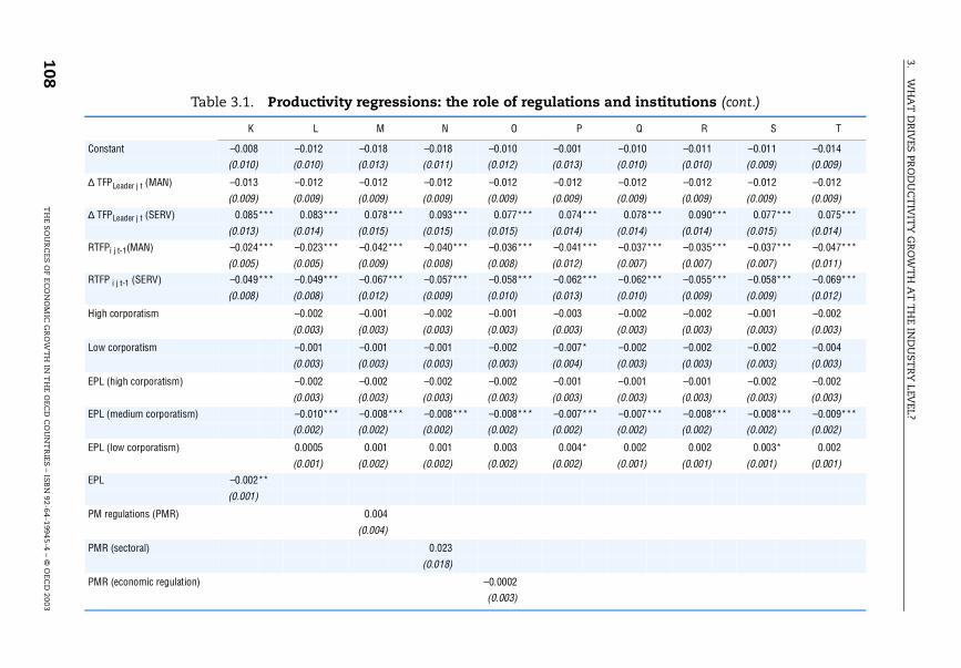
3.W
HA
T D
RIV
ES PR
OD
UC
TIV
ITY
GR
OW
TH
AT
TH
E IND
UST
RY
LEVEL?
108T
HE S
OU
RC
ES O
F EC
ON
OM
IC G
RO
WT
H IN
TH
E OEC
D C
OU
NT
RIES – ISB
N 92-64-19945-4 – ©
OEC
D 2003
s and institutions (cont.)
Q R S T
–0.010 –0.011 –0.011 –0.014
(0.010) (0.010) (0.009) (0.009)
–0.012 –0.012 –0.012 –0.012
(0.009) (0.009) (0.009) (0.009)
** 0.078*** 0.090*** 0.077*** 0.075***
(0.014) (0.014) (0.015) (0.014)
** –0.037*** –0.035*** –0.037*** –0.047***
(0.007) (0.007) (0.007) (0.011)
** –0.062*** –0.055*** –0.058*** –0.069***
(0.010) (0.009) (0.009) (0.012)
–0.002 –0.002 –0.001 –0.002
(0.003) (0.003) (0.003) (0.003)
–0.002 –0.002 –0.002 –0.004
(0.003) (0.003) (0.003) (0.003)
–0.001 –0.001 –0.002 –0.002
(0.003) (0.003) (0.003) (0.003)
** –0.007*** –0.008*** –0.008*** –0.009***
(0.002) (0.002) (0.002) (0.002)
0.002 0.002 0.003* 0.002
(0.001) (0.001) (0.001) (0.001)
Table 3.1. Productivity regressions: the role of regulation
K L M N O P
Constant –0.008 –0.012 –0.018 –0.018 –0.010 –0.001
(0.010) (0.010) (0.013) (0.011) (0.012) (0.013)
∆ TFPLeader j t (MAN) –0.013 –0.012 –0.012 –0.012 –0.012 –0.012
(0.009) (0.009) (0.009) (0.009) (0.009) (0.009)
∆ TFPLeader j t (SERV) 0.085*** 0.083*** 0.078*** 0.093*** 0.077*** 0.074*
(0.013) (0.014) (0.015) (0.015) (0.015) (0.014)
RTFPi j t-1(MAN) –0.024*** –0.023*** –0.042*** –0.040*** –0.036*** –0.041*
(0.005) (0.005) (0.009) (0.008) (0.008) (0.012)
RTFP i j t-1 (SERV) –0.049*** –0.049*** –0.067*** –0.057*** –0.058*** –0.062*
(0.008) (0.008) (0.012) (0.009) (0.010) (0.013)
High corporatism –0.002 –0.001 –0.002 –0.001 –0.003
(0.003) (0.003) (0.003) (0.003) (0.003)
Low corporatism –0.001 –0.001 –0.001 –0.002 –0.007*
(0.003) (0.003) (0.003) (0.003) (0.004)
EPL (high corporatism) –0.002 –0.002 –0.002 –0.002 –0.001
(0.003) (0.003) (0.003) (0.003) (0.003)
EPL (medium corporatism) –0.010*** –0.008*** –0.008*** –0.008*** –0.007*
(0.002) (0.002) (0.002) (0.002) (0.002)
EPL (low corporatism) 0.0005 0.001 0.001 0.003 0.004*
(0.001) (0.002) (0.002) (0.002) (0.002)
EPL –0.002**
(0.001)
PM regulations (PMR) 0.004
(0.004)
PMR (sectoral) 0.023
(0.018)
PMR (economic regulation) –0.0002
(0.003)
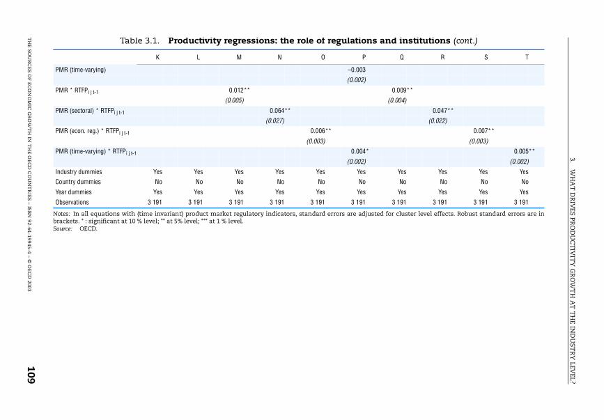
3.W
HA
T D
RIV
ES PRO
DU
CT
IVIT
Y G
RO
WT
H A
T T
HE IN
DU
STR
Y LEV
EL?
TH
E SOU
RC
ES OF EC
ON
OM
IC G
RO
WT
H IN
TH
E OEC
D C
OU
NT
RIES
– ISB
N 92-64-19945-4 – ©
OE
CD
2003109
Table 3.1. Productivity regressions: the role of regulations and institutions (cont.)
sted for cluster level effects. Robust standard errors are in
Q R S T
0.009**
(0.004)
0.047**
(0.022)
0.007**
(0.003)
0.005**
(0.002)
Yes Yes Yes Yes
No No No No
Yes Yes Yes Yes
3 191 3 191 3 191 3 191
Notes: In all equations with (time invariant) product market regulatory indicators, standard errors are adjubrackets. * : significant at 10 % level; ** at 5% level; *** at 1 % level.Source: OECD.
K L M N O P
PMR (time-varying) –0.003
(0.002)
PMR * RTFPi j t-1 0.012**
(0.005)
PMR (sectoral) * RTFPi j t-1 0.064**
(0.027)
PMR (econ. reg.) * RTFPi j t-1 0.006**
(0.003)
PMR (time-varying) * RTFPi j t-1 0.004*
(0.002)
Industry dummies Yes Yes Yes Yes Yes Yes
Country dummies No No No No No No
Year dummies Yes Yes Yes Yes Yes Yes
Observations 3 191 3 191 3 191 3 191 3 191 3 191
3. WHAT DRIVES PRODUCTIVITY GROWTH AT THE INDUSTRY LEVEL?
Box 3.3. Indicators of the stringency of product market regulations and employment protection legislation
In the empirical analysis, three types of indicators of product marketregulations and one on particular aspects of labour market regulationsare considered (for more details, see Scarpetta et al., 2002).
The overall index of the stringency of product market regulation (PMR)is a static indicator computed for the year 1998. It consists of threeelements: i) direct state control of economic activities, through stateshareholdings or other types of intervention in the decisions of businesssector enterprises and the use of command and control regulations;ii) barriers to private entrepreneurial activity, through legal limitationson access to markets, or administrative burdens and opacitieshampering the creation of businesses; and iii) regulatory barriers tointernational trade and investment, through explicit legal and tariff
provisions or regulatory and administrative obstacles (see Nicoletti et al.,1999 for more details). The indicator has a wide coverage of regulatoryaspects, but neither industry nor time dimension. In order to furthercharacterise the regulatory settings, this indicator is further split intotwo components: economic regulations (state control, legal barriers toentry, etc.) and administrative regulations (administrative burdens onstart-ups, features of the licensing and permit system, etc.).
The industry-specific indicator of product regulation (PMR sectoral) is alsoa static indicator (1998), but it varies across service-sector industries (retailand wholesale trade; transport and communication; financialintermediation and business services). The indicator always includesbarriers to entrepreneurial activity and public ownership, while for certainindustries it also considers other aspects of regulation. For themanufacturing industries, for which no specific information on regulationsis available, the economy-wide indicator of administrative regulations isused as a proxy in the construction of this sector-specific indicator.1
The aggregate time-varying indicator of the stance of regulation (PMR time-varying) is a simple average of time-varying indicators of the stringencyof regulations in electricity and gas, as well as in transport and
communication. This average is used to proxy the overall stance ofregulatory reform in each OECD country. Its clear advantage in theempirical analysis is the time dimension but, given that it only coverscertain (albeit key) service industries, it should be considered as a firstapproximation of the economy-wide regulatory reform stance of OECD
countries (see Nicoletti et al., 2001 for more details).
110 THE SOURCES OF ECONOMIC GROWTH IN THE OECD COUNTRIES – ISBN 92-64-19945-4 – © OECD 2003
3. WHAT DRIVES PRODUCTIVITY GROWTH AT THE INDUSTRY LEVEL?
found to influence productivity in either highly centralised/co-ordinated ordecentralised countries. One potential explanation is that technologicalchange is often associated with skill upgrading of the workforce. The requiredadjustment of the workforce can be achieved either using the internal labour
market via firm-sponsored training if EPL is strict, or by acquiring thenecessary skills on the external labour market. In this context, strict EPL raisesthe costs of adjusting the workforce. The implied detrimental effect ontechnology adoption may be magnified in the intermediate regime, where thecosts of adjusting the workforce are sufficiently high to deter firms from usingthe external labour market, while at the same time the lack of co-ordinationdoes not offer them the required institutional device to guarantee a highreturn on internal training, because other firms can poach on their skilledworkforce by offering higher wages.21
The empirical results can be restated in terms of the potential effects ofpolicy reforms on the long-run level of multifactor productivity.22 Bearing inmind the illustrative nature of such an exercise, a reduction in the stringencyof product market regulations is estimated to substantially reduce theproductivity gap in countries such as Greece, Portugal and Spain over thelonger run. This assessment only takes into account the indirect effect ofregulatory reform on the process of technology adoption, but does not include
Box 3.3. Indicators of the stringency of product market regulations and employment protection legislation (cont.)
The indicators of employment protection legislation are available fortwo periods (late 1980s and 1998) and focus on both regular andtemporary contracts (see Nicoletti et al. 1999). Regulations for regularcontracts include: i) procedural inconvenience that employers face whentrying to dismiss a worker; ii) advance notice of dismissal and severancepayments; and iii) prevailing standards of, and penalties for, “unfair”
dismissals. Indicators of the stringency of EPL for temporary contractsinclude: i) the “objective” reasons under which they can be offered; ii) themaximum number of successive renewals; and iii) the maximumcumulated duration of the contract. The EPL indicator used in theeconometric analysis is time-varying, with the shift in regime from thelate 1980s stance to that of 1990s being defined on the basis ofinformation about the timing of major EPL reforms (concerning bothtemporary and regular workers) in OECD countries.
1. The indicator of administrative regulations is used as a proxy instead of the overallindicator of product market regulations because it refers to norms and regulations that areapplied to all industries, while the overall indicator also includes economic regulations,some of which are more sector-specific and do not apply to manufacturing industries.
THE SOURCES OF ECONOMIC GROWTH IN THE OECD COUNTRIES – ISBN 92-64-19945-4 – © OECD 2003 111
3. WHAT DRIVES PRODUCTIVITY GROWTH AT THE INDUSTRY LEVEL?
the potential effect of such a reform on increased R&D activity. An easing of
employment protection legislation may also significantly boost productivity,at least in countries – such as Belgium, France or Portugal – where theadjustments costs associated to EPL are not offset by the possibility ofadjusting wages or use of internal training.
Another topic of interest relates to the possible influence of sector- ormarket-specific conditions on the productivity generating process. This issue
can be investigated using manufacturing data, for which appropriatestatistical information on market structures and technology regimes can becomputed. As detailed in Box 3.4, manufacturing industries may be classifiedinto two broad categories: low-tech (LT in Table 3.2) and high-tech industries(HT). Table 3.2 presents the (preferred) equations estimated to explorewhether the productivity impact of the technology gap, and also that of R&D,depend on these technology regimes and market characteristics. The resultspoint to a strong and highly significant effect of the technology catch-up for LTindustries, while this effect is not statistically significant in high-techindustries. However, this latter group is rather heterogeneous and equation Iin the table further decomposes it into two groups: high concentration (HTHC)and low concentration (HTLC). The results suggest a significant convergence
in high-concentrated high-tech industries, but no convergence in low-concentrated industries. These findings are consistent with the idea thatindustries operating in low-tech industries tend to share the same technology,so that spillover effects may be significant. In contrast, such spillover effectsare likely to be less marked when the evolution of technology stimulatesproduct or process diversification, as is the case in industries operating in amonopolistic competition regime (HTLC).
The results also enable refinement of the analysis of the links betweenpolicy and institutional variables and productivity. In particular, the inclusionof R&D in the productivity equation for manufacturing implies that the direct
effect of product market regulations is only marginally significant (equation E)and, if control EPL is also included, the effect is no longer statisticallysignificant. However, the indirect effect via the technology gap remainssignificant.
Table 3.2 also indicates a differentiated effect of R&D on productivity,depending on the technology regime.23 Indeed, if allowed to vary betweenlow- and high-tech industries, the estimated effect of R&D becomesinsignificant in the latter. As in the case of technology convergence, however,this result hides a different behaviour of industries depending on whethertheir technology regime leads to low or high concentration (see last column ofTable 3.2). Indeed, there is no significant effect of R&D on productivity in low-concentrated high-tech industries, but a strong effect in high-concentratedindustries. High-tech industries with low concentration are often
112 THE SOURCES OF ECONOMIC GROWTH IN THE OECD COUNTRIES – ISBN 92-64-19945-4 – © OECD 2003
3. WHAT DRIVES PRODUCTIVITY GROWTH AT THE INDUSTRY LEVEL?
characterised by “creative destruction” with technological ease of entry and a
major role played by new firms in innovative activities (see also Nelson andWinter, 1982). Thus, returns on R&D in these industries may not be long-lasting, and R&D is likely to be driven by the need to engage in (perceived)product differentiation to maintain/acquire market shares. In this context,high R&D intensity may not necessarily result in higher measured productivity,unless quality differentiation is taken into account in measuring industryvalue-added, which is the case of only a few industries in a very fewcountries.24 By contrast, high-tech but concentrated industries are generallycharacterised by “creative accumulation”, with the prevalence of large,established firms and the presence of barriers for new innovators. Returns toR&D in these industries are, therefore, likely to be larger than in lowconcentration ones, possibly leading to persistent technological leadership.25
This latter point is reinforced by the positive sign of the interaction termbetween R&D and the technology gap. This implies greater returns from R&Dof leading firms compared with followers. Indeed, knowledge andtechnological progress is strongly cumulative in these industries, oftenproviding the technological leader with a “first-mover advantage” in theintroduction of innovations.
Indirect determinants of multi-factor productivity via R&D activity
Albeit differentiated by technology regimes, the empirical analysispresented in the previous section has clearly indicated the importance of R&Dactivity for productivity. It is, therefore, important to assess whetherregulation and institutional settings also influence productivity indirectly viatheir impact on R&D activity.26 As discussed above, both theoretical andempirical studies lend some support to the idea that, for a given level ofproperty rights, strict regulatory settings that undermine competition maycurb incentives to engage in innovation. Likewise, a few studies have arguedthat high costs of adjusting the workforce may have important consequencesfor the profitability of firms’ innovative strategies.
A simple model of the determinants of innovative effort relates the latterto expected profit differential – i.e. the expected difference between profitsthat the firm can earn once it has successfully innovated, and those thatwould be earned otherwise.27 Regulations in both product and labour marketsmay affect the expected profit differential. Hence, taking the ratio of business-performed R&D expenditure to sales (hereafter R&D intensity) as the indicator
of innovative activity, a reduced-form R&D equation can be expressed as afunction on regulations and a set of other control variables (such as humancapital or the degree of protection of intellectual property rights).
The indicators of product market regulation include measures of statecontrol and administrative regulation (administrative barriers on start-ups,
THE SOURCES OF ECONOMIC GROWTH IN THE OECD COUNTRIES – ISBN 92-64-19945-4 – © OECD 2003 113
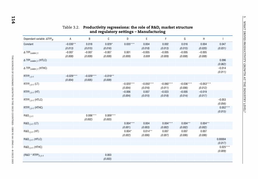
3.W
HA
T D
RIV
ES PR
OD
UC
TIV
ITY
GR
OW
TH
AT
TH
E IND
UST
RY
LEVEL?
114T
HE S
OU
RC
ES O
F EC
ON
OM
IC G
RO
WT
H IN
TH
E OEC
D C
OU
NT
RIES – ISB
N 92-64-19945-4 – ©
OEC
D 2003
, market structure ring
F G H I
0.002 0.016 0.004 0.047(0.013) (0.015) (0.020) (0.031)–0.005 –0.005 –0.005(0.009) (0.008) (0.008)
0.096(0.062)–0.014(0.011)
–0.060*** –0.036*** –0.053***(0.011) (0.006) (0.012)–0.023 –0.005 –0.019(0.018) (0.014) (0.017)
–0.053(0.056)
0.052***(0.015)
0.004*** 0.004** 0.004**(0.002) (0.002) (0.002)
0.007 0.007 0.007(0.007) (0.006) (0.006)
0.00004(0.017)
0.025***(0.009)
Table 3.2. Productivity regressions: the role of R&Dand regulatory settings – Manufactu
Dependant variable: ∆TFPijt A B C D E
Constant –0.030** 0.018 0.029* 0.035*** 0.004(0.013) (0.015) (0.016) (0.018)
∆ TFPLeader j t –0.007 –0.007 –0.007 0.001 –0.005(0.008) (0.009) (0.009) (0.009) 0.009
∆ TFPLeader j t (HTLC)
∆ TFPLeader j t (HTHC)
RTFPi j t-1 –0.029*** –0.029*** –0.019**(0.004) (0.005) (0.009)
RTFPi j t-1 (LT) –0.020*** –0.050***(0.004) (0.016)
RTFPi j t-1 (HT) –0.006 0.007(0.004) (0.015)
RTFPi j t-1 (HTLC)
RTFPi j t-1 (HTHC)
R&Di j t-1 0.006*** 0.009***(0.002) (0.003)
R&Di j t-1 (LT) 0.004*** 0.004(0.001) (0.003)
R&Di j t-1 (HT) 0.004* 0.014**(0.002) (0.006)
R&Di j t-1 (HTLC)
R&Di j t-1 (HTHC)
(R&D * RTFP)i j t-1 0.003(0.003)
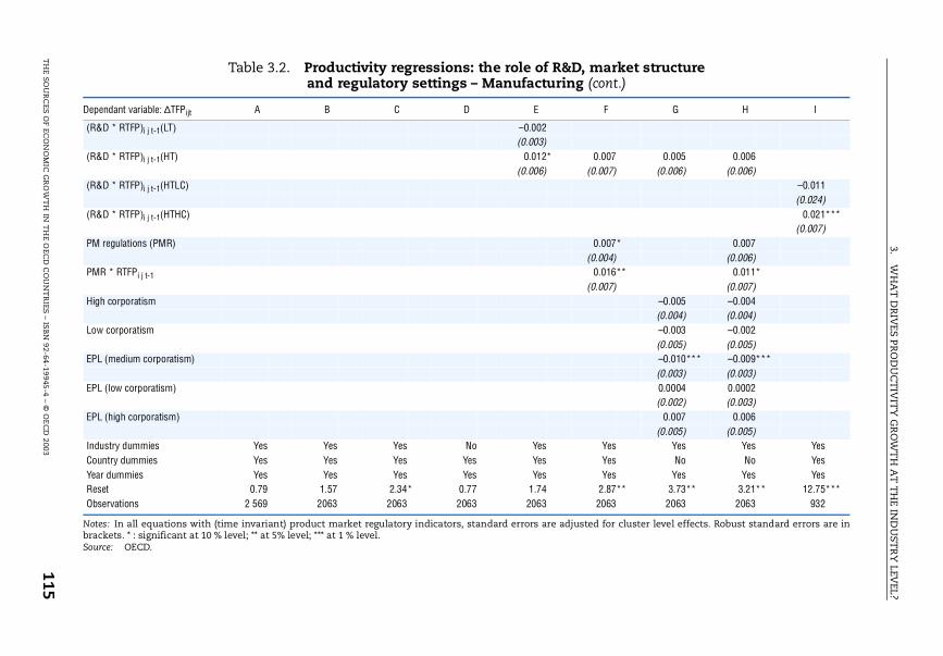
3.W
HA
T D
RIV
ES PRO
DU
CT
IVIT
Y G
RO
WT
H A
T T
HE IN
DU
STR
Y LEV
EL?
TH
E SOU
RC
ES OF EC
ON
OM
IC G
RO
WT
H IN
TH
E OEC
D C
OU
NT
RIES
– ISB
N 92-64-19945-4 – ©
OE
CD
2003115
Table 3.2. Productivity regressions: the role of R&D, market structure (cont.)
sted for cluster level effects. Robust standard errors are in
F G H I
0.007 0.005 0.006(0.007) (0.006) (0.006)
–0.011(0.024)
0.021***(0.007)
0.007* 0.007(0.004) (0.006)
0.016** 0.011*(0.007) (0.007)
–0.005 –0.004(0.004) (0.004)–0.003 –0.002(0.005) (0.005)–0.010*** –0.009***(0.003) (0.003)0.0004 0.0002(0.002) (0.003)
0.007 0.006(0.005) (0.005)
Yes Yes Yes YesYes No No YesYes Yes Yes Yes
2.87** 3.73** 3.21** 12.75***2063 2063 2063 932
and regulatory settings – Manufacturing
Notes: In all equations with (time invariant) product market regulatory indicators, standard errors are adjubrackets. * : significant at 10 % level; ** at 5% level; *** at 1 % level.Source: OECD.
Dependant variable: ∆TFPijt A B C D E
(R&D * RTFP)i j t-1(LT) –0.002(0.003)
(R&D * RTFP)i j t-1(HT) 0.012*(0.006)
(R&D * RTFP)i j t-1(HTLC)
(R&D * RTFP)i j t-1(HTHC)
PM regulations (PMR)
PMR * RTFPi j t-1
High corporatism
Low corporatism
EPL (medium corporatism)
EPL (low corporatism)
EPL (high corporatism)
Industry dummies Yes Yes Yes No YesCountry dummies Yes Yes Yes Yes YesYear dummies Yes Yes Yes Yes YesReset 0.79 1.57 2.34* 0.77 1.74Observations 2 569 2063 2063 2063 2063
3. WHAT DRIVES PRODUCTIVITY GROWTH AT THE INDUSTRY LEVEL?
Box 3.4. A taxonomy of manufacturing industries according to their technology regimes
The industrial organisation literature suggests three main elementscharacterising market conditions across industries. First, differences inmarket power may relate to differences in entry barriers, due toexogenous technological conditions such as economies of scale(see e.g. Panzar, 1989) and scope (Baumol et al., 1982). Second, it has beenargued that entry barriers may result from high sunk costs rather than
from economies of scale. Finally, more recent research has focused onhorizontal and vertical product differentiation (Eaton and Lipsey, 1989).Products can be considered as differentiated vertically when consumerscan rank them by quality, otherwise they can be viewed as differentiatedhorizontally.
In practice, the possible combinations of these three dimensions,
according to their relative importance, lead to a reduced number ofmarket structure prototypes. In practical terms, Sutton (2000) offers asimple market structure classification into three categories, based on thereturns to innovation and the degree of market concentration:
Low-tech industries (LT): if the returns to innovation are low,investment in R&D will be low, and the industry will typically produce
fairly standardised goods with little or no monopoly rents. Thisconfiguration is indicated by LT in the equations presented in Table 3.2.
High-tech industries, low concentration (HTLC): if the returns toinnovation are high, firms will invest heavily in technologies thatimprove process and products. However, if the evolution of technologyleads to alternative types of products (product differentiation) or
processes, there will typically be a large number of producers, eachwith some market power but little monopoly rents due to free entry ofnew firms to produce new (differentiated) products. Such marketstructure comes close to so-called (Chamberlain’s) monopolisticcompetition. The motor vehicle industry may be considered a goodexample of such type of manufacturing industry.
High-tech industries, high concentration (HTHC): in contrast to theprevious case, if high returns to innovation can only be attained alonga single trajectory, (high-tech) firms will inevitably move towards ahighly-concentrated market structure, in which a small number ofplayers dominate the market. Parts of the information andcommunication technology industry (e.g. software) may be consideredgood examples of this type of manufacturing industry.
116 THE SOURCES OF ECONOMIC GROWTH IN THE OECD COUNTRIES – ISBN 92-64-19945-4 – © OECD 2003
3. WHAT DRIVES PRODUCTIVITY GROWTH AT THE INDUSTRY LEVEL?
feature of the licensing and permit system, etc), indicators of tariff and non-tariff barriers, plus an indicator of global protection of intellectual property
rights (IPRs).28 Import penetration is used as a proxy for competitive pressuresnot captured by the regulatory indicators. A control for the average size offirms captures the possible bias in R&D intensity across industries andcountries due to different accounting practices between large and small firmsand has been proved to play an important role in the l iterature(see e.g. Griliches, 1990, Geroski, 1990).
Choosing a log-linear form for convenience, the R&D equation can beexpressed as follows:
where the dependent variable is the average R&D intensity in a given country/industry, IMP and SIZE denote import penetration and average size, µ standsfor the country dummy, χ stands for the industry dummy, ε is the standarderror term, while h, i and j index product market regulatory indicators,countries and industries, respectively.
Equation [3.5] is estimated on a cross-section of 18 manufacturingindustries in 18 OECD countries.29 The choice of a cross-section – rather thanpanel data, as in the case of the productivity equation – is justified by the needto include a set of control variables for which the time dimension is lacking,including certain aspects of product market regulations. The underlying dataare the same as those used in the MFP equation above, except that here allvariables have been averaged across the period 1993-1997.30 In addition,industrial relations and technology regimes are considered, in order to explorethe potential interactions between these two variables and employment
protection legislation in explaining R&D expenditures.
The results are presented in Table 3.3. The estimated models account forthe effects of EPL, industrial relations regimes and their potential interactions,
Box 3.4. A taxonomy of manufacturing industries according to their technology regimes (cont.)
The nature of competition, the impact of given policy and institutionalsettings and, ultimately, economic performance may vary across thesedifferent market structures. For example, high mark-ups could be takenas a sign of market power in industries with low R&D, although they maywell be an indication of innovation rents in those with high R&D (OliveiraMartins and Scarpetta, 1999). Similarly, high R&D expenditure may not
result in high productivity growth, but rather in higher market shares inmarkets with highly differentiated products.
ijjiijijh
h
ijhij SIZEIMPPMRDR εχµδφγα ++++++= ∑&log [3.5]
THE SOURCES OF ECONOMIC GROWTH IN THE OECD COUNTRIES – ISBN 92-64-19945-4 – © OECD 2003 117
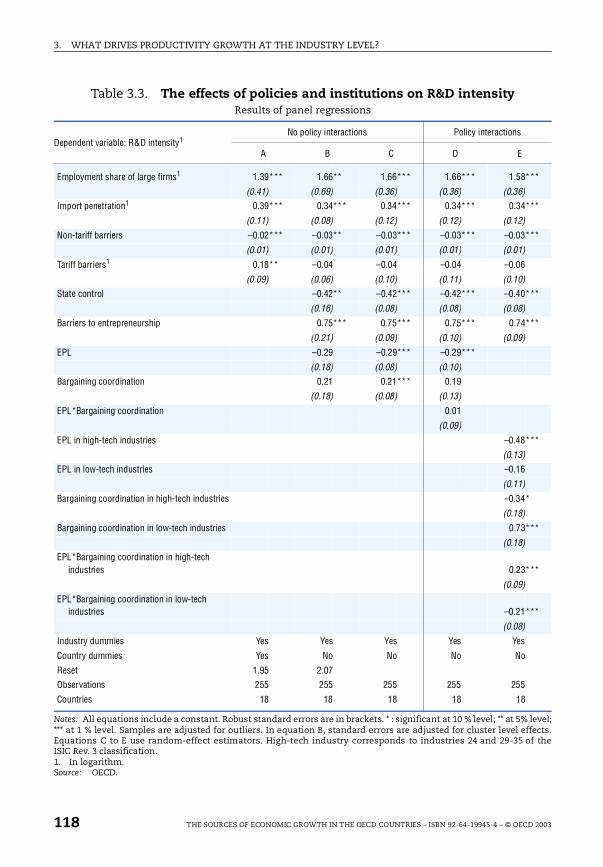
3. WHAT DRIVES PRODUCTIVITY GROWTH AT THE INDUSTRY LEVEL?
level;ects.f the
**
**
**
**
**
**
**
**
**
Table 3.3. The effects of policies and institutions on R&D intensityResults of panel regressions
Notes: All equations include a constant. Robust standard errors are in brackets. * : significant at 10 % level; ** at 5% *** at 1 % level. Samples are adjusted for outliers. In equation B, standard errors are adjusted for cluster level effEquations C to E use random-effect estimators. High-tech industry corresponds to industries 24 and 29-35 oISIC Rev. 3 classification.1. In logarithm.Source: OECD.
Dependent variable: R&D intensity1No policy interactions Policy interactions
A B C D E
Employment share of large firms1 1.39*** 1.66** 1.66*** 1.66*** 1.58*
(0.41) (0.69) (0.36) (0.36) (0.36)
Import penetration1 0.39*** 0.34*** 0.34*** 0.34*** 0.34*
(0.11) (0.08) (0.12) (0.12) (0.12)
Non-tariff barriers –0.02*** –0.03** –0.03*** –0.03*** –0.03*
(0.01) (0.01) (0.01) (0.01) (0.01)
Tariff barriers1 0.18** –0.04 –0.04 –0.04 –0.06
(0.09) (0.06) (0.10) (0.11) (0.10)
State control –0.42** –0.42*** –0.42*** –0.40*
(0.16) (0.08) (0.08) (0.08)
Barriers to entrepreneurship 0.75*** 0.75*** 0.75*** 0.74*
(0.21) (0.09) (0.10) (0.09)
EPL –0.29 –0.29*** –0.29***
(0.18) (0.08) (0.10)
Bargaining coordination 0.21 0.21*** 0.19
(0.18) (0.08) (0.13)
EPL*Bargaining coordination 0.01
(0.09)
EPL in high-tech industries –0.48*
(0.13)
EPL in low-tech industries –0.16
(0.11)
Bargaining coordination in high-tech industries –0.34*
(0.18)
Bargaining coordination in low-tech industries 0.73*
(0.18)
EPL*Bargaining coordination in high-tech industries 0.23*
(0.09)
EPL*Bargaining coordination in low-tech industries –0.21*
(0.08)
Industry dummies Yes Yes Yes Yes Yes
Country dummies Yes No No No No
Reset 1.95 2.07
Observations 255 255 255 255 255
Countries 18 18 18 18 18
118 THE SOURCES OF ECONOMIC GROWTH IN THE OECD COUNTRIES – ISBN 92-64-19945-4 – © OECD 2003
3. WHAT DRIVES PRODUCTIVITY GROWTH AT THE INDUSTRY LEVEL?
but control also for outward and inward-oriented product market regulations
(at both the industry and economy-wide levels). In addition, they control forfirm size (the share of employment in large enterprises) and trade openness(proxied by import penetration).31 All regressions also include industryd u mm i es to c ontr ol fo r u nexp la i ned ind us try cha rac ter i s t ics(e.g. technological opportunity). Finally, the potential interaction between EPL,industrial relations regimes and the technological characteristics of differentindustries was dealt with by introducing a dummy variable that identifieshigh-technology industries (see above).
The empirical results confirm the positive association between recordedR&D intensity and the average size of firms in each industry. Moroever, R&Dactivity tends to increase with trade openness, perhaps pointing to theexistence of positive knowledge spillovers. Indeed, trade openness tends toincrease product variety in domestic markets and induces imitation bydomestic producers and the latter often requires spending in R&D (Cohen andLevinthal, 1989). The degree of protection of IPRs also appears to be positively,and significantly, associated with R&D intensity in all specifications.32
Concerning the role of regulations, the results point to an unambiguousnegative effect of non-tariff barriers and state control on R&D. By contrast,trade tariffs as well barriers to entrepreneurship are positively associated withR&D intensity. The different impact of tariffs and non-tariff barriers on R&D isconsistent with some theoretical considerations. While from a partialequilibrium point of view trade restrictions tend to add to foreign competitors’costs without changing the incentive to innovate amongst domestic firms, in
general equilibrium, they also curb imports and possible knowledge spilloversrelated to them. This latter effect is likely to be stronger for non-tariff barriersthan for tariffs because they have greater impact on the diffusion of productsand, eventually, the possibility of imitation by domestic firms.33 The positiveassociations between barriers to entrepreneurship and R&D might be due tothe fact that these barriers, by discouraging entry, may contribute toincreasing ex post innovation rents and improving appropriability conditions,reinforcing the effect of IPRs protection.
R&D intensity also appears to decrease with the stringency of EPL and toincrease with the degree of co-ordination. At the same time, no effect on R&Dof the interaction between EPL and co-ordination in industrial relations can befound pooling all industries together. Results change, however, if separatecoefficients for high- and low-technology industries are estimated: interactionterms now have significant and opposite effects on the two sets of industries.At any given level of EPL and co-ordination in industrial relations, theircombination appears to have a positive effect on R&D intensity in high-techindustries and a negative effect in low-tech industries. The rationale for thisresult is that in low-tech industries the scope for expansion is often limited
THE SOURCES OF ECONOMIC GROWTH IN THE OECD COUNTRIES – ISBN 92-64-19945-4 – © OECD 2003 119
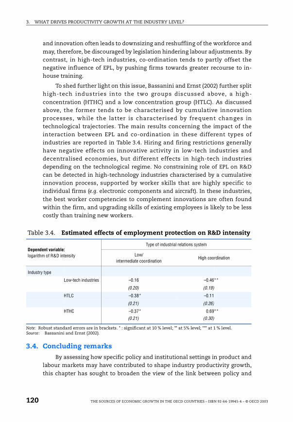
3. WHAT DRIVES PRODUCTIVITY GROWTH AT THE INDUSTRY LEVEL?
and innovation often leads to downsizing and reshuffling of the workforce and
may, therefore, be discouraged by legislation hindering labour adjustments. Bycontrast, in high-tech industries, co-ordination tends to partly offset thenegative influence of EPL, by pushing firms towards greater recourse to in-house training.
To shed further light on this issue, Bassanini and Ernst (2002) further splithigh-tech industries into the two groups discussed above, a high-
concentration (HTHC) and a low concentration group (HTLC). As discussedabove, the former tends to be characterised by cumulative innovationprocesses, while the latter is characterised by frequent changes intechnological trajectories. The main results concerning the impact of theinteraction between EPL and co-ordination in these different types ofindustries are reported in Table 3.4. Hiring and firing restrictions generallyhave negative effects on innovative activity in low-tech industries anddecentralised economies, but different effects in high-tech industriesdepending on the technological regime. No constraining role of EPL on R&Dcan be detected in high-technology industries characterised by a cumulativeinnovation process, supported by worker skills that are highly specific toindividual firms (e.g. electronic components and aircraft). In these industries,
the best worker competencies to complement innovations are often foundwithin the firm, and upgrading skills of existing employees is likely to be lesscostly than training new workers.
3.4. Concluding remarks
By assessing how specific policy and institutional settings in product andlabour markets may have contributed to shape industry productivity growth,
this chapter has sought to broaden the view of the link between policy and
Table 3.4. Estimated effects of employment protection on R&D intensity
Note: Robust standard errors are in brackets. * : significant at 10 % level; ** at 5% level; *** at 1 % level.Source: Bassanini and Ernst (2002).
Dependent variable: logarithm of R&D intensity
Type of industrial relations system
Low/intermediate coordination
High coordination
Industry type
Low-tech industries –0.16 –0.46**
(0.20) (0.19)
HTLC –0.38* –0.11
(0.21) (0.26)
HTHC –0.37* 0.69**
(0.21) (0.30)
120 THE SOURCES OF ECONOMIC GROWTH IN THE OECD COUNTRIES – ISBN 92-64-19945-4 – © OECD 2003
3. WHAT DRIVES PRODUCTIVITY GROWTH AT THE INDUSTRY LEVEL?
growth tackled in Chapter 2. Most prominently, there is evidence that
stringent regulatory settings in the product market, as well as strictemployment legislation, have a negative bearing on productivity at theindustry – and, therefore, macro – levels. However, these policy influences arenot straightforward, and depend on a number of factors.
The impact of regulations and institutions on performance varies,depending on the market and technology conditions in which it is operating.
In particular, the burden of strict product market regulations on productivityseems to be greater the larger the technological gap with the industry/countryleader: strict regulation hinders the adoption of existing technologies, possiblybecause it reduces competitive pressures or technology spillovers. In addition,strict product market regulations also have a negative impact on the processof innovation itself (insofar as it can be proxied by R&D expenditure). Thus,given the strong impact of R&D on productivity, there is also an indirectchannel whereby strict product market regulations may reduce the scope forproductivity enhancement.
The link between employment protection legislation and productivity isalso complex. There is evidence to suggest that high hiring and firing costsweaken productivity performance, especially when they are not offset bywages and/or internal training, thereby inducing sub-optimal adjustments ofthe workforce to technology changes and innovation. These considerationsare consistent with the firm-level evidence (see Ahn, 2001, for a survey)suggesting that the effects on productivity of innovation and adoption of newtechnologies are enhanced in firms with a highly-skilled workforce or with
strong investment in training.
Finally, there is considerable variation in the effect of R&D activity onproductivity, depending on market structures and technology regimes. Forexample, there is some support to the idea that strong R&D activity does notnecessarily bring about higher productivity when firms are engaged in strongproduct differentiation and when there are different possible technology
trajectories. In turn, the impact of hiring and firing costs on R&D depends onindustrial relations and technology regimes. For example, while EPL adds tothe negative effects on innovation of strict product market regulations inunco-ordinated countries and in low-tech industries, in high-tech industrieswith cumulative innovation process the effect is not marked.
These results offer some insights to the observed multi-factor
productivity growth differentials seen at the aggregate level (see Chapter 1).Indeed, most of the countries having experienced a slow-down in multi-factorproductivity growth during the 1990s are characterised by strict productmarket regulation, as well as by strict employment protection legislationcombined with wage-settings that do not offset the associated high labour
THE SOURCES OF ECONOMIC GROWTH IN THE OECD COUNTRIES – ISBN 92-64-19945-4 – © OECD 2003 121

3. WHAT DRIVES PRODUCTIVITY GROWTH AT THE INDUSTRY LEVEL?
adjustment costs. Moreover, the evidence concerning interactions between
labour market policies, industrial relations systems and technologicalcharacteristics suggests that in countries with high bargaining co-ordinationand relatively strict EPL (e.g. Germany, Austria), innovative activity is likely tothrive in industries characterised by a dominant technology and a cumulativeinnovation process. Countries that have a decentralised bargaining systemand more lax EPL (e.g. the United States) are better equipped to innovate inindustries characterised by multiple and rapidly-evolving technologies,including most of the ICT industry.
However, despite providing some clues to the reasons behind thedifferent size of the ICT industry and, more generally, the widening gap inmulti-factor productivity growth across OECD countries, this chapter has leftunanswered a number of key issues. More specifically, it has not tackled thedeterminants of firms’ behaviour, which has played a major role in enhancingtechnological progress over the recent period. Chapter 4 aims at filling thisgap, by analysing the role of firm turnover for aggregate productivity growthand the main determinants of entry, exit and post-entry expansion of firms.
Notes
1. This chapter draws from Scarpetta and Tressel (2002).
2. The shift-share analysis is performed using the maximum industrydecomposition available in ISDB-STAN: 3-4 digit ISIC for manufacturing (i.e. a22 industry detail), and 2-digit ISIC for services. This decomposition bears severallimitations other than the lack of detail for services (Timmer and Szirmai, 1999).First, it focuses on labour productivity and not on multi-factor productivity.Second, it assumes that marginal productivity of factor inputs moving in or out ofan industry is the same as average productivity. Finally, if output growth ispositively related to productivity growth (the so-called Verdoorn effect), theimpact of structural change may be underestimated, since part of the shift torapid-growth sectors will be counted in the within-effect.
3. It was particularly important in the United Kingdom in the 1980s, where it waslinked to the decline of mining and manufacturing.
4. Given the limited disaggregation of the service sector available, it is possible thatconsiderable structural changes occurring within some broadly defined industries(e.g. business services) pass unnoticed. However, further investigation using USdata does not lend much support to this view. Indeed, to shed light on thesensitivity of the decomposition of between and within effects to changes in theindustry details, the shift-share analysis was replicated for the United States withthree different industry breakdowns provided by the Bureau of Economic Analysis:1) 1-digit data; 2) details for manufacturing but broad aggregates for services andmining (i.e. close to the decomposition used in the text); and 3) the maximumdetail of 58 industries. The results did not show a high sensitivity of thedecomposition to the degree of industry detail used, confirming the strong role ofwithin-industry changes in productivity in explaining aggregate patterns.
122 THE SOURCES OF ECONOMIC GROWTH IN THE OECD COUNTRIES – ISBN 92-64-19945-4 – © OECD 2003
3. WHAT DRIVES PRODUCTIVITY GROWTH AT THE INDUSTRY LEVEL?
5. It should be stressed, however, that there are many dimensions of intellectualproperty rights legislation, some of which could have ambiguous effects on R&Dactivity. See OECD (2001a) for more details.
6. For a brief overview of existing studies, see Scarpetta and Tressel (2002).
7. For cross-country studies that explore the role of competition on productivityusing mark-ups and concentration indexes, see Cheung and Garcia Pascual (2001).
8. For studies using firms’ market shares, see Nickell (1996), Nickell et al. (1997) andDisney et al. (2000).
9. For example, Boone (2000a) suggests that there may be a hump-shapedrelationship between competition and mark-ups.
10. For instance, well-designed policies can provide insurance against the risk of jobloss, improve matching and commitment in worker-firm relationships andencourage skill upgrading.
11. See amongst others, Audretsch and Thurik (2001), Caroli et al. (2001), Hobjin andJovanovic (2001).
12. This is the main assumption behind most theoretical and empirical studies,which both emphasise the importance of R&D for productivity (see e.g. Griliches,1990; Griliches and Lichtenberg, 1984; and recently Guellec and van Pottelsberghe,2001).
13. See for instance Cohen and Levinthal (1989) or Griffith et al. (2000).
14. See Soskice (1997), Eichengreen and Iversen (1999), Acemoglu and Pischke(1999a,b).
15. As shown in Box 3.2, product market regulations are assumed to affect the level,not the growth rate, of MFP.
16. For example, if the adoption of new technologies relies partly on new firms, highentry barriers may reduce the pace of adoption (see e.g. Boone, 2000b).
17. See Annex 5 for a detailed presentation of countries, industries and data sources.
18. As indicated by equation [3.4] in Box 3.2, all equations control for country, industryand year fixed effects. Since there is evidence of heteroscedasticity in the data, theHuber-White-Sandwich estimator is used for standard errors. All equationsexclude a number of outlier observations identified on the basis of the DFIT andCOVRATIO statistical tests. These observations significantly increase the standarderror of the regression, or affect the estimated coefficients (see Chatterjee andHadi, 1988). For further details on econometric issues involved in the equationspresented in this chapter (model selection, residual tests, specification tests,identification of outliers, etc.), see Scarpetta and Tressel (2002).
19. These results are broadly consistent with those of other studies by Blundell et al.(1995, 1999), Nickell (1996) and Cheung and Garcia Pascual (2001).
20. The summary indicator of the bargaining system (corporatism) combines twovariables: i) the level of bargaining: centralised, intermediate (at sector orregional), or decentralised (firm level); and ii) the degree of co-ordination amongst,on the one hand, employers’ associations and, on the other, trade unions. Thiscombined variable allows consideration of cases where co-operation betweenemployers and unions in an industry bargaining setting (e.g., Germany and Austriaand, more recently, Italy, Ireland, the Netherlands with the income policyagreements) may be an alternative, or functionally equivalent, to centralised
THE SOURCES OF ECONOMIC GROWTH IN THE OECD COUNTRIES – ISBN 92-64-19945-4 – © OECD 2003 123
3. WHAT DRIVES PRODUCTIVITY GROWTH AT THE INDUSTRY LEVEL?
systems, thereby mimicking their outcomes. In the table, the two variablesreferring to corporatism indicate the effects of high/low centralisation/co-ordination with respect to that of an intermediate system. The distribution ofcountries according to the different aspects of collective bargaining and changesover time is presented in Elmeskov, Martin and Scarpetta (1998).
21. Unlike decentralised or intermediate – i.e. where sectoral wage-bargaining ispredominant without co-ordination – regimes, a centralised and/or co-ordinatedbargaining system offers an institutional device that discourages poaching, andthus favours internal training: i) contracts tend to cover a large fraction ofemployers and workers in most industries with limited room for differences inwage offers across industries which, in turn, reduces incentives for highly-skilledworkers to change job (Teulings and Hartog, 1998; Acemoglu and Pischke, 1999a);ii) in such a regime, poaching may be considered as unfair behaviour (Blinder andKrueger, 1996; Casper et al.,1999); and finally iii) the cost of training is often sharedamong employers when business associations have a prominent role (Soskice,1997, Casper et al., 1999).
22. See Annex 3 for details.
23. It should be stressed that despite the large number of studies, the links betweenR&D activity and market structure remain the subject of intense discussion (see,amongst others, Symeonidis, 1996 for a survey).
24. See Annex 1. However, even if quality differences could be fully measured, firms inhighly product-differentiated markets may still be caught in a process of R&Descalation, leading to a rise in R&D expenditures but not necessarily higherproductivity (Sutton, 1996).
25. These two groups of high-tech industries have also been labelled SchumpeterianMark I and Mark II industries (see Malerba and Orsenigo, 1995, 1997, for anexhaustive characterisation of these technological regimes). See Scarpetta et al.,2002 for details on the separation of industries into these two groups.
26. For all details on the issues and results treated below, see Bassanini andErnst (2002).
27. See e.g. Aghion et al. (2001a); Boone (2000b); Aghion et al. (2001b).
28. The indicator of IPR is based on national intellectual property legislation ascalculated by Ginarte and Park (1997). They use five point score based on the sumof five national components: i) τηε extent of coverage (pharmaceuticals, food, etc.);ii) membership in international agreements; iii) loss of protection (compulsorylicense provisions, etc.); iv) enforcement mechanisms (provisions for injunctions,pleadings, etc.); and v) duration of protection. Walter Park kindly provided thesedata.
29. See Bassanini and Ernst (2002) and Nicoletti et al. (2001) for more details.
30. The very few exceptions to this rule are detailed in Bassanini and Ernst (2002).
31. Firm size is often found to correlate with R&D intensity, but the direction ofcausation is unclear. This link may simply be the outcome of different accountingpractices between large and small firms (Griliches, 1990), but it could also reflectthe fact that successful innovation typically leads to larger firm size (Dasguptaand Stiglitz, 1980; Levin and Reiss, 1984; and Sutton, 1998). In any event, it isimportant to stress that all the results described below are essentially robust tothe elimination of the control for firm size from the estimated modelspecification.
124 THE SOURCES OF ECONOMIC GROWTH IN THE OECD COUNTRIES – ISBN 92-64-19945-4 – © OECD 2003

3. WHAT DRIVES PRODUCTIVITY GROWTH AT THE INDUSTRY LEVEL?
32. Results concerning protection of IPRs must be taken with care as the coefficient ofthis variable is likely to be overestimated due to the endogeneity of the indicatorto the level of R&D expenditure (see Ginarte and Park, 1997).
33. Moreover, high non-tariff barriers can be thought to affect directly the elasticity ofsubstitution between imported and domestically-produced products, therebyinducing low incentives to innovate when domestic and foreign firms have similarlevels of competitiveness (the case of “neck and neck” competition see Aghionet al. 1997, 2001a; and Boone, 2000b).
THE SOURCES OF ECONOMIC GROWTH IN THE OECD COUNTRIES – ISBN 92-64-19945-4 – © OECD 2003 125
ISBN 92-64-19945-4
The Sources of Economic Growth in the OECD Countries© OECD 2003
Chapter 4
Firm Dynamics, Productivity and Policy Settings
Abstract. This last chapter moves one step further in the examinationof the policy determinants of economic growth by exploiting a new firm-level database for ten OECD countries. It shows that the contribution toproductivity growth from firm dynamic processes should not beoverlooked, most notably in high-tech industries where new firms tend toboost overall productivity. There is evidence that burdensome regulationson entrepreneurial activity as well as high costs of adjusting the workforcenegatively affect the entry of new small firms. Overall, there are a numberof different features of entrant and exiting firms across countries. Inparticular, in the United States entrant firms tend to be smaller and withlower than average productivity, but those which survive the initial yearsexpand rapidly. By contrast, firms tend to enter with a relatively highersize and productivity in Europe, but subsequently do not expandsignificantly. These findings tend to support the hypothesis of greatermarket experimentation in the United States, compared to manycontinental European countries, which in turn is likely to be the result ofdifferences in regulatory settings across the Atlantic.
THE SOURCES OF ECONOMIC GROWTH IN THE OECD COUNTRIES – ISBN 92-64-19945-4 – © OECD 2003 127
4. FIRM DYNAMICS, PRODUCTIVITY AND POLICY SETTINGS
Introduction
Chapter 3 focused on industry-level productivity and innovation andtheir dependence on policy and regulatory settings in the product and labourmarkets. This chapter makes a further step into the analysis of the micro-determinants of economic growth, by focussing on the contribution ofreallocation of resources within narrowly-defined industries, resulting fromthe expansion of more productive firms and the entry of new firms, as well asthe exit of obsolete ones. This aspect of reallocation may vary greatly acrosscountries and has often been considered as a sign of economic dynamism. In
particular, it has been argued that overall growth is usually associated withnew entrants who displace obsolescent firms, and that this “creativedestruction” contributes to overall technological progress, as new firms maybetter harness new technologies (Box 4.1). Moreover, by increasingcompetitive pressures, (the threat of) new entries may indirectly stimulatetechnological progress, even when productivity growth apparently takes placewithin incumbent firms.
The main task of this chapter is threefold. First it assesses thecontribution of firm dynamics to industry-level productivity growth(Section 4.1). As such, it is the first attempt in the micro-economic literature tostudy the role of firm dynamics and its main characteristics for a relativelylarge set of countries and, more importantly, on the basis of harmonised data.Since firm dynamics seems to play an important role as a driver ofproductivity, the chapter then characterises this process in differentindustries and countries (Section 4.2). This evidence allows testing of some ofthe stylised facts presented in previous papers (e.g. Geroski 1995, Caves 1998)which were generally formulated with reference to very few countries. The
analysis attempts to control for the sectoral composition of the economy, so asto isolate cross-country differences that may be related to differences ininstitutional and regulatory settings. Section 4.3 looks at the evolution offirms after market entry. The final task of the chapter is to further develop theanalysis of policy influences on long-term growth (Section 4.4). This is done byassessing whether some of the regulatory settings in product and labourmarkets discussed in the previous chapter (with reference to overall industryMFP) also influence firm dynamics. In turn, this analysis sheds further light onone particular channel through which regulations may affect aggregateperformance, namely via their negative impact on entry rates.
128 THE SOURCES OF ECONOMIC GROWTH IN THE OECD COUNTRIES – ISBN 92-64-19945-4 – © OECD 2003
4. FIRM DYNAMICS, PRODUCTIVITY AND POLICY SETTINGS
Box 4.1. “Creative Destruction”, firm dynamics and economic growth
In the recent past, micro-evidence has accumulated to suggest a wideheterogeneity of firms’ behaviour in most markets.1 The distribution ofoutput, employment, investment and productivity across firms andestablishments varies widely; even in expanding industries, many firmsexperience substantial decline, and in contracting industries it is notuncommon to find rapidly expanding units. Likewise, business-cycle
upturns and downturns do not necessarily involve a synchronisedmovement of all, or even most, firms or establishments.
There are a number of possible explanations for this. Heterogeneitymay, for instance, reflect certain product market conditions, e.g. productdifferentiation. At the same time, and arguably more importantly,heterogeneity may be associated with a continual shift in the
composition of the population of firms through entry, exit, expansionand contraction. This process of “creative destruction” (a notion usuallyascribed to Joseph Schumpeter) may be important in developing andcreating new processes, products and markets and, hence, in fosteringoverall economic growth.2
Various explanations have been formulated to describe the
Schumpeterian process of “creative destruction”. One group ofexplanations focuses on the learning process (either active or passive) offirms. Uncertainty about market conditions and profitability may, indeed,lead firms to make different choices concerning technologies, goods andproduction facilities. In the passive learning approach (Jovanovic, 1982) a firmenters a market without knowing its given potential profitability ex ante.Only after entry does the firm start to learn about its own profitability, basedon information from realised profits. By continually updating such learning,the firm decides to expand, contract or exit. One of the main implications ofthis model is that smaller and younger firms should have higher and morevariable growth rates. In the active learning approach (Ericson and Pakes,1995) a firm actively explores its economic environment and invests in
order to enhance its profitability under competitive pressure from bothwithin and outside the industry. Its profitability changes over time inresponse to the outcomes of the firm’s own investment and those of otheractors in the same market. The firm grows if successful and shrinks or exitsif not. In any event, because of the inherent uncertainty in experimentation,even an entrant who is very successful, ex post, will typically begin small.The accumulation of experience and assets, in turn, strengthens survivorsand lowers the likelihood of failure.
THE SOURCES OF ECONOMIC GROWTH IN THE OECD COUNTRIES – ISBN 92-64-19945-4 – © OECD 2003 129
4. FIRM DYNAMICS, PRODUCTIVITY AND POLICY SETTINGS
4.1. What lies behind within-industry productivity growth? Reallocation of resources versus within-firm growth
Chapter 3 has shown that overall productivity gains result predominantlyfrom an intra-industry effect. The following natural step is, therefore, to lookinside different industries to assess how the reallocation of resources amongincumbents, as well as between entrants and exiters, shapes industryproductivity growth. This process of “creative destruction”, whereby newentrants displace obsolescent firms, may be especially important in thecurrent period of diffusion of a new general purpose technology, such as ICT.
Methodological issues
The analysis presented in this Section offers a consistent internationalcomparison of firm dynamics and its contribution to aggregate productivity,through the use of specially-constructed firm-level data (Box 4.2) for ten OECDcountries (United States, Germany, France, Italy, United Kingdom, Canada,Denmark, Finland, Netherlands and Portugal). These harmonised data areused below to assess the role of entry and exit and reallocation amongstexisting firms in total productivity growth. Notwithstanding the efforts madeto minimise inconsistencies along different dimensions (e.g. sectoral
Box 4.1. “Creative Destruction”, firm dynamics and economic growth (cont.)
A second group of explanations of the “creative-destruction” processstresses that new technology is often embodied in new capital, whichrequires a costly retooling process in existing plants adopting thesetechnologies, as well as in some cases changing work practices.3 Insofaras new firms do not have to go through this process, they may betterharness new technologies. Hence, overall growth will be associated with
new entrants who displace obsolete establishments.4 In this case, theprocess of “creative destruction” also contributes to the observedheterogeneity in firms’ performance, to the extent that some sunk costsimpede the exit of oldest and least productive firms.
1. For a survey of recent empirical studies see Caves (1998) and Bartelsman and Doms (2000).2. For analyses of “creative destruction” and its links with economic growth, see, amongst
others, Aghion and Howitt (1992) and Caballero and Hammour (1994, 1996). Foster,Haltiwanger and Krizan (1998), Caves (1998) and Bartelsman and Doms (2000) offer furtherdiscussion on this literature.
3. For such vintage models of technological change, see for instance Cooley et al. (1997), andJensen et al. (2001).
4. Models emphasising such a strong link between economic growth and the process of entryand exit include Caballero and Hammour (1994), Mortensen and Pissarides (1994) andCampbell (1997).
130 THE SOURCES OF ECONOMIC GROWTH IN THE OECD COUNTRIES – ISBN 92-64-19945-4 – © OECD 2003
4. FIRM DYNAMICS, PRODUCTIVITY AND POLICY SETTINGS
Box 4.2. Building up a consistent international dataset: the OECD firm-level study1
Sources of data
Available data at the firm level are usually compiled for fiscal andother purposes and, unlike macroeconomic data, there are fewinternationally agreed definitions and sources, although harmonisationhas improved over the years (see Annex 3 for more details on the OECDfirm-level project).
The analysis of firm entry and exit is based on business registers(Canada, Denmark, France, Finland, Netherlands, the United Kingdomand the United States) or social security databases (Germany and Italy).Data for Portugal are drawn from an employee-based register containinginformation on both establishments and firms. These databases allowfirms to be tracked over time because addition or removal of some ofthem from the registers (at least in principle) reflects their actual entryand exit. The decomposition of aggregate productivity growth requires(in this chapter) a wider set of variables and is based on productionsurvey data, in combination with business registers.
Definition of key concepts
The entry rate is defined as the number of new firms divided by thetotal number of incumbent and entrant firms in a given year; the exit rate
is defined as the number of firms exiting the market in a given yeardivided by the population of origin, i.e. the incumbents in the previousyear.
Labour productivity growth is defined as the difference between the rateof growth of output and that of employment2 and, whenever possible,controls for material inputs.
Multi-factor productivity growth is the change in gross output less theshare weighted changes in three different inputs:3 labour, measured by
the number of employed persons; capital, based on the perpetualinventory method; and, material inputs. Real values for output arecalculated by applying 2-4 digit industry deflators.
Comparability issues
Two prominent aspects of the data have to be borne in mind whencomparing firm-level data across countries:4
Unit of observation: the data used in this study refer to “firms’ ratherthan “establishments”. Firm-based data are likely to more closely
THE SOURCES OF ECONOMIC GROWTH IN THE OECD COUNTRIES – ISBN 92-64-19945-4 – © OECD 2003 131
4. FIRM DYNAMICS, PRODUCTIVITY AND POLICY SETTINGS
breakdown, time horizon, definition of entry and exit, etc.), some remainingdifferences have to be taken into account when interpreting the results.
At the industry level, productivity growth is the result of differentcombinations of: i) productivity gains within existing firms; ii) increases in themarket-share of high-productivity firms; and iii) the entry of new firms thatdisplace less productive ones. Productivity growth within firms depends onchanges in the efficiency and intensity with which inputs are used inproduction. Thus, this source of aggregate productivity growth is associatedwith the process of technological progress. Shifts in market shares betweenhigh and low productive units also affect aggregate productivity trends, as
does the reallocation of resources across entering and exiting firms. Theoverall contribution of reallocation to productivity growth is generallyidentified with a competitive process taking place in the market, although it
Box 4.2. Building up a consistent international dataset: the OECD firm-level study1 (cont.)
represent entities that are responsible for key aspects of decision-making, compared with plant-level data. Nevertheless, businessregisters may define firms at different points in ownership structures;for example, some registers consider firms that are effectivelycontrolled by a “parent” firm as separate units, whilst others recordonly the parent company.5
Size threshold: while some registers include even single-personbusinesses, others omit firms smaller than a certain size, usually interms of the number of employees but sometimes in terms of othermeasures, such as sales (as is the case in the data for France and Italy).Data used in this book exclude single-person businesses. However,because smaller firms tend to have more volatile firm dynamics,
remaining differences in the threshold across different countrydatasets should be taken into account in the internationalcomparison.6
1. A subset of the firm-level data is available on the OECD’s website at: www.oecd.org/EN/document/0,,EN-document-492-nodirectorate-no-1-35177-3,00.html
2. Available data do not allow the control for changes in hours worked, nor do they distinguishbetween part- and full-time employment.
3. Changes are calculated at the firm level but income shares refer to the industry average inorder to minimise measurement errors.
4. For more detail on the comparability of the firm-level data, see Bartelsman et al., (2002).5. This may not be a major shortcoming in practice, judging from US data. Indeed, when
repeating the decomposition of productivity growth for the United States on the basis ofestablishment instead of firm data, the results remain largely unchanged.
6. This may also not be a major shortfall in practice: a sensitivity analysis on Finnish data,where cut-off points were set at 5 and 20 employees, reveals broadly similar results.
132 THE SOURCES OF ECONOMIC GROWTH IN THE OECD COUNTRIES – ISBN 92-64-19945-4 – © OECD 2003
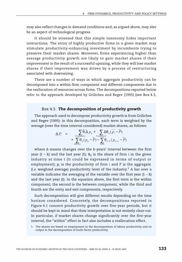
4. FIRM DYNAMICS, PRODUCTIVITY AND POLICY SETTINGS
may also reflect changes in demand conditions and, as argued above, may also
be an aspect of technological progress.
It should be stressed that this simple taxonomy hides importantinteractions. The entry of highly productive firms in a given market maystimulate productivity-enhancing investment by incumbents trying topreserve their market shares. Moreover, firms experiencing higher thanaverage productivity growth are likely to gain market shares if their
improvement is the result of a successful upsizing, while they will lose marketshares if their improvement was driven by a process of restructuringassociated with downsizing.
There are a number of ways in which aggregate productivity can bedecomposed into a within-firm component and different components due tothe reallocation of resources across firms. The decompositions reported below
refer to the approach developed by Griliches and Regev (1995) (see Box 4.3,
Box 4.3. The decomposition of productivity growth
The approach used to decompose productivity growth is from Grilichesand Regev (1995): in this decomposition, each term is weighted by theaverage (over the time interval considered) market shares, as follows:
where ∆ means changes over the k-years’ interval between the firstyear (t − k) and the last year (t); θit is the share of firm i in the givenindustry at time t (it could be expressed in terms of output oremployment); pi is the productivity of firm i and P is the aggregate(i.e. weighted average) productivity level of the industry.1 A bar over avariable indicates the averaging of the variable over the first year (t – k)and the last year (t). In the equation above, the first term is the withincomponent; the second is the between component, while the third andfourth are the entry and exit components, respectively.
Such decomposition will give different results depending on the timehorizon considered. Concretely, the decompositions reported inFigure 4.1 concern productivity growth over five-year periods, but itshould be kept in mind that their interpretation is not entirely clear-cut.In particular, if market shares change significantly over the five-yearinterval, the “within” effect in fact also includes a reallocation effect.
1. The shares are based on employment in the decomposition of labour productivity and onoutput in the decomposition of multi-factor productivity.
)()(
)(
PpPp
PppP
kit
Exits
kitit
Entries
it
Continuers
iitit
Continuers
it
−−−+
−∆+∆=∆
−−∑∑∑∑
θθ
θθ
THE SOURCES OF ECONOMIC GROWTH IN THE OECD COUNTRIES – ISBN 92-64-19945-4 – © OECD 2003 133
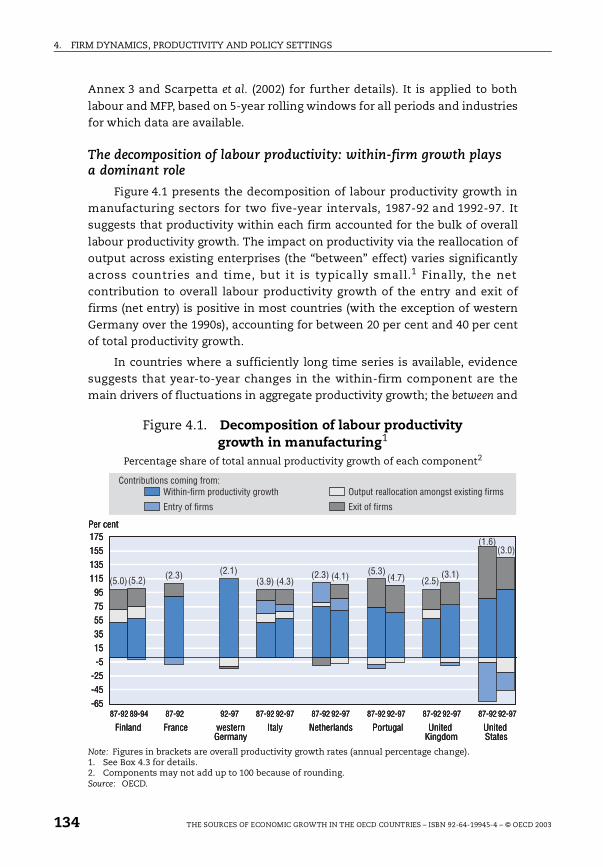
4. FIRM DYNAMICS, PRODUCTIVITY AND POLICY SETTINGS
Annex 3 and Scarpetta et al. (2002) for further details). It is applied to both
labour and MFP, based on 5-year rolling windows for all periods and industriesfor which data are available.
The decomposition of labour productivity: within-firm growth plays a dominant role
Figure 4.1 presents the decomposition of labour productivity growth inmanufacturing sectors for two five-year intervals, 1987-92 and 1992-97. Itsuggests that productivity within each firm accounted for the bulk of overall
labour productivity growth. The impact on productivity via the reallocation ofoutput across existing enterprises (the “between” effect) varies significantlyacross countries and time, but it is typically small.1 Finally, the netcontribution to overall labour productivity growth of the entry and exit offirms (net entry) is positive in most countries (with the exception of westernGermany over the 1990s), accounting for between 20 per cent and 40 per centof total productivity growth.
In countries where a sufficiently long time series is available, evidencesuggests that year-to-year changes in the within-firm component are themain drivers of fluctuations in aggregate productivity growth; the between and
Figure 4.1. Decomposition of labour productivity growth in manufacturing1
Percentage share of total annual productivity growth of each component2
Note: Figures in brackets are overall productivity growth rates (annual percentage change).1. See Box 4.3 for details.2. Components may not add up to 100 because of rounding.Source: OECD.
1751551351159575553515-5
-25-45-65
87-92 89-94 87-92 92-97 87-92 92-97 87-92 92-97 87-92 92-97 87-92 92-97 87-92 92-97
(5.0)(5.2) (2.3) (2.1)(3.9) (4.3)
(2.3) (4.1) (5.3)(4.7) (2.5)
(3.1)
(1.6)(3.0)
Within-firm productivity growthContributions coming from:
Output reallocation amongst existing firms
Entry of firms Exit of firms
Per cent
Finland France westernGermany
Italy Netherlands Portugal United Kingdom
United States
134 THE SOURCES OF ECONOMIC GROWTH IN THE OECD COUNTRIES – ISBN 92-64-19945-4 – © OECD 2003

4. FIRM DYNAMICS, PRODUCTIVITY AND POLICY SETTINGS
net entry components show only modest fluctuations (see Annex 3 for more
details). Consequently, in years of expansion (the second half of the 1980s inmost countries), within-firm growth makes a stronger contribution to overallproductivity growth, whereas in slowdowns (the early 1990s) the contributionof between and net entry components increase in relative importance,2
particularly because of the exit of low-productive units.
The entry of new firms has variable effects on overall productivity growth.
On the whole, data for European countries3 show that new firms typically makea positive contribution to overall productivity growth (see Table 4.1), althoughthe effect is generally of small magnitude. By contrast, entries make a negativecontribution in the United States for most industries. Instead a strongcontribution to productivity growth in the United States comes from the exit oflow-productivity firms. This finding is consistent with further evidence that ispresented below, indicating a somewhat different nature of the entry (and exit)process in the United States compared with most other countries.
Table 4.1. Analysis of productivity components across industries of manufacturing and services
Panel A. Proportions of positive contributions to labour productivity growth across manufacturing industries1
Panel B. Proportions of positive contributions to labour productivity growth across business services1
Note: These calculations are based on all available data with manufacturing and business services. Thetime periods considered vary considerably across countries.
1. Number of cases in which the different components made a positive contribution to labourproductivity growth (in % of total number of cases).
Source: OECD.
Total number of observations (industry * year)
Entry contribution %
Exit contribution %
Between component %
Finland 420 57 93 62
France 126 47 81 40
Italy 348 84 89 85
Netherlands 344 76 77 51
Portugal 211 63 91 49
United Kingdom 392 62 92 45
United States 58 10 98 31
Total number of observations(industry * year)
Entry contribution %
Exit contribution %
Between component %
Finland 24 50 79 46
western Germany 18 56 71 50
Italy 227 30 54 29
Portugal 191 39 66 43
THE SOURCES OF ECONOMIC GROWTH IN THE OECD COUNTRIES – ISBN 92-64-19945-4 – © OECD 2003 135
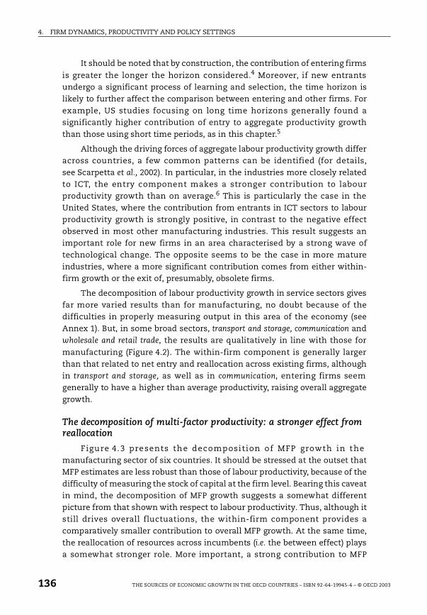
4. FIRM DYNAMICS, PRODUCTIVITY AND POLICY SETTINGS
It should be noted that by construction, the contribution of entering firms
is greater the longer the horizon considered.4 Moreover, if new entrantsundergo a significant process of learning and selection, the time horizon islikely to further affect the comparison between entering and other firms. Forexample, US studies focusing on long time horizons generally found asignificantly higher contribution of entry to aggregate productivity growththan those using short time periods, as in this chapter.5
Although the driving forces of aggregate labour productivity growth differacross countries, a few common patterns can be identified (for details,see Scarpetta et al., 2002). In particular, in the industries more closely relatedto ICT, the entry component makes a stronger contribution to labourproductivity growth than on average.6 This is particularly the case in theUnited States, where the contribution from entrants in ICT sectors to labourproductivity growth is strongly positive, in contrast to the negative effectobserved in most other manufacturing industries. This result suggests animportant role for new firms in an area characterised by a strong wave oftechnological change. The opposite seems to be the case in more matureindustries, where a more significant contribution comes from either within-firm growth or the exit of, presumably, obsolete firms.
The decomposition of labour productivity growth in service sectors givesfar more varied results than for manufacturing, no doubt because of thedifficulties in properly measuring output in this area of the economy (seeAnnex 1). But, in some broad sectors, transport and storage, communication andwholesale and retail trade, the results are qualitatively in line with those for
manufacturing (Figure 4.2). The within-firm component is generally largerthan that related to net entry and reallocation across existing firms, althoughin transport and storage, as well as in communication, entering firms seemgenerally to have a higher than average productivity, raising overall aggregategrowth.
The decomposition of multi-factor productivity: a stronger effect from reallocation
Figure 4.3 presents the decomposition of MFP growth in themanufacturing sector of six countries. It should be stressed at the outset thatMFP estimates are less robust than those of labour productivity, because of thedifficulty of measuring the stock of capital at the firm level. Bearing this caveatin mind, the decomposition of MFP growth suggests a somewhat differentpicture from that shown with respect to labour productivity. Thus, although itstill drives overall fluctuations, the within-firm component provides acomparatively smaller contribution to overall MFP growth. At the same time,the reallocation of resources across incumbents (i.e. the between effect) playsa somewhat stronger role. More important, a strong contribution to MFP
136 THE SOURCES OF ECONOMIC GROWTH IN THE OECD COUNTRIES – ISBN 92-64-19945-4 – © OECD 2003
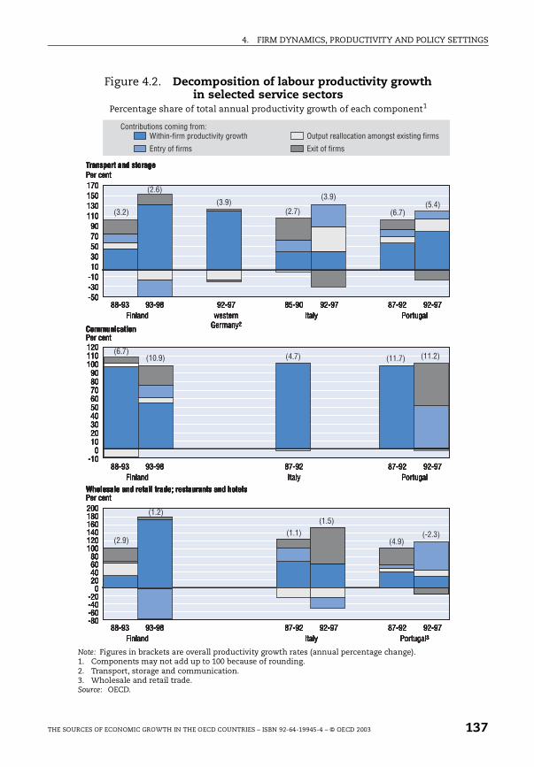
4. FIRM DYNAMICS, PRODUCTIVITY AND POLICY SETTINGS
Figure 4.2. Decomposition of labour productivity growth in selected service sectors
Percentage share of total annual productivity growth of each component1
Note: Figures in brackets are overall productivity growth rates (annual percentage change).1. Components may not add up to 100 because of rounding.2. Transport, storage and communication.3. Wholesale and retail trade.Source: OECD.
1701501301109070503010
-10-30-50
1201101009080706050403020100
-10
88-93 93-98 92-97 85-90 92-97 87-92 92-97
200180160140120100806040200
-20-40-60-80
(3.2)
(6.7)
(2.9)
(1.2)
(1.1)(1.5)
(4.9)(-2.3)
(10.9) (4.7) (11.7) (11.2)
(2.6)
(3.9)(2.7)
(3.9)
(6.7)(5.4)
Within-firm productivity growthContributions coming from:
Output reallocation amongst existing firms
Entry of firms Exit of firms
Transport and storagePer cent
CommunicationPer cent
Wholesale and retail trade; restaurants and hotelsPer cent
Finland westernGermany2
Italy Portugal
88-93 93-98 87-92 87-92 92-97Finland Italy Portugal
88-93 93-98 87-92 87-92 92-9792-97Finland Italy Portugal3
THE SOURCES OF ECONOMIC GROWTH IN THE OECD COUNTRIES – ISBN 92-64-19945-4 – © OECD 2003 137
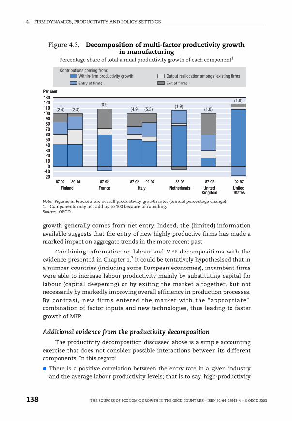
4. FIRM DYNAMICS, PRODUCTIVITY AND POLICY SETTINGS
growth generally comes from net entry. Indeed, the (limited) informationavailable suggests that the entry of new highly productive firms has made amarked impact on aggregate trends in the more recent past.
Combining information on labour and MFP decompositions with theevidence presented in Chapter 1,7 it could be tentatively hypothesised that in
a number countries (including some European economies), incumbent firmswere able to increase labour productivity mainly by substituting capital forlabour (capital deepening) or by exiting the market altogether, but notnecessarily by markedly improving overall efficiency in production processes.By contrast, new firms entered the market with the “appropriate”combination of factor inputs and new technologies, thus leading to fastergrowth of MFP.
Additional evidence from the productivity decomposition
The productivity decomposition discussed above is a simple accountingexercise that does not consider possible interactions between its differentcomponents. In this regard:
There is a positive correlation between the entry rate in a given industry
and the average labour productivity levels; that is to say, high-productivity
Figure 4.3. Decomposition of multi-factor productivity growth in manufacturing
Percentage share of total annual productivity growth of each component1
Note: Figures in brackets are overall productivity growth rates (annual percentage change).1. Components may not add up to 100 because of rounding.Source: OECD.
130120110100
908070605040302010
0-10-20
87-92 89-94 87-92 87-92 92-97 88-93 87-92 92-97
(2.4) (2.8)(0.9)
(4.9) (5.3)(1.9)
(1.8)
(1.6)
Within-firm productivity growth Output reallocation amongst existing firms
Entry of firms Exit of firms
Per cent
Finland France Italy Netherlands United Kingdom
United States
Contributions coming from:
138 THE SOURCES OF ECONOMIC GROWTH IN THE OECD COUNTRIES – ISBN 92-64-19945-4 – © OECD 2003

4. FIRM DYNAMICS, PRODUCTIVITY AND POLICY SETTINGS
industries are associated with relatively high entry rates. This may reflect
new firms putting competitive pressure on incumbents, or highlyproductive industries attracting more entrants.
Within each country, high-productivity industries tend to have a widerdispersion of productivity levels than other industries. Specifically, whilemost industries, regardless of their aggregate level of productivity, have anumber of relatively low productive firms, high overall productivity in some
industries is largely driven by the presence of “exceptional” performers thatlengthen the right-hand tail of the distribution of industry productivity.
4.2. The entry and exit of firms
Since the entry and exit of firms makes a significant – albeit notdominant – contribution to aggregate productivity growth, it is of interest tosee how frequently new firms are created and how often existing units closedown. In fact, a large number of firms enter and exit most markets every year(Panel A of Figure 4.4). Data covering the first part of the 1990s show firmturnover rates (entry plus exit rates) to be around 20 per cent in the businesssector of most countries (Panel B of Figure 4.4): i.e. a fifth of firms are eitherrecent entrants, or will close down within the year.
The industry dimension also makes it possible to compare entry and exitrates and characterise turnover. If entries were driven by relatively high profitsin a given industry, and exits occurred primarily in sectors with relatively lowprofits, there would be a negative cross-sectional correlation between entryand exit rates. However, confirming previous evidence,8 entry and exit ratesare generally highly correlated across industries in OECD countries (this isparticularly so when the rates are weighted by employment) (Table 4.2). Thisfinding suggests a process of “creative destruction”, whereby a large numberof new firms displace continuously a large number of obsolete firms.
The variability of turnover rates for the same industry across countries iscomparable in magnitude to that across industries in each country. In otherwords, the observed variability of turnover across countries can be explainedboth by industry-specific and country-specific effects.
It is possible to assess these country-specific effects by estimating entryrates for each country once differences in the sectoral composition are takeninto account, by means of (fixed-effects) panel regression.9 Overall, Figure 4.5suggests a similar degree of “firm churning” in Europe and the United States:with the exception of western Germany and Italy, all countries have higherentry rates than the United States, but differences are small and would, infact, be even smaller if the different size structure of firms across countrieswere taken into account.10
THE SOURCES OF ECONOMIC GROWTH IN THE OECD COUNTRIES – ISBN 92-64-19945-4 – © OECD 2003 139
4. FIRM DYNAMICS, PRODUCTIVITY AND POLICY SETTINGS
Figure 4.4. High firm turnover rates in OECD countriesEntry and exit rates,1 annual average, 1989-1994
1. The entry rate is the ratio of entering firms to the total population. The exit rate is the ratio ofexiting firms to the population of origin. Turnover rates are the sum of entry and exit rates.
2. Total economy minus agriculture and community services.Source: OECD.
20
16
12
8
4
0
24
20
16
12
8
4
0Netherlands western
GermanyItaly Finland France Denmark Portugal Canada United
StatesUnited
Kingdom
Italy Denmark westernGermany
Finland Netherlands Canada France UnitedStates
Portugal
Entry rates Exit rates
Per cent
Panel A. Entry and exit rates in total business sector2
Business sector2 Manufacturing Business service sector
Per cent
Panel B. Overall firm turnover in broad sectors
20
16
12
8
4
0
24
20
16
12
8
4
0Netherlands western
GermanyItaly Finland France Denmark Portugal Canada United
StatesUnited
Kingdom
Italy Denmark westernGermany
Finland Netherlands Canada France UnitedStates
Portugal
Entry rates Exit rates
Per cent
Panel A. Entry and exit rates in total business sector2
Business sector2 Manufacturing Business service sector
Per cent
Panel B. Overall firm turnover in broad sectors
140 THE SOURCES OF ECONOMIC GROWTH IN THE OECD COUNTRIES – ISBN 92-64-19945-4 – © OECD 2003
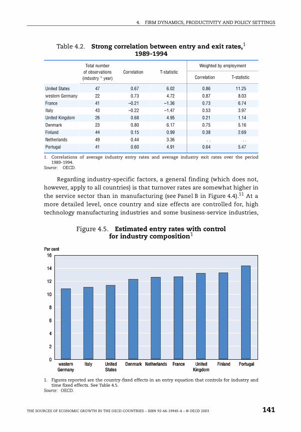
4. FIRM DYNAMICS, PRODUCTIVITY AND POLICY SETTINGS
Regarding industry-specific factors, a general finding (which does not,however, apply to all countries) is that turnover rates are somewhat higher in
the service sector than in manufacturing (see Panel B in Figure 4.4).11 At amore detailed level, once country and size effects are controlled for, hightechnology manufacturing industries and some business-service industries,
Table 4.2. Strong correlation between entry and exit rates,1 1989-1994
1. Correlations of average industry entry rates and average industry exit rates over the period1989-1994.
Source: OECD.
Total number of observations(industry * year)
Correlation T-statisticWeighted by employment
Correlation T-statistic
United States 47 0.67 6.02 0.86 11.25
western Germany 22 0.73 4.72 0.87 8.03
France 41 –0.21 –1.36 0.73 6.74
Italy 43 –0.22 –1.47 0.53 3.97
United Kingdom 26 0.68 4.95 0.21 1.14
Denmark 23 0.80 6.17 0.75 5.16
Finland 44 0.15 0.99 0.38 2.69
Netherlands 49 0.44 3.36 . . . .
Portugal 41 0.60 4.91 0.64 5.47
Figure 4.5. Estimated entry rates with control for industry composition1
1. Figures reported are the country-fixed effects in an entry equation that controls for industry andtime fixed effects. See Table 4.5.
Source: OECD.
0
16
14
12
10
8
6
4
2
Per cent
westernGermany
Italy UnitedStates
Denmark Netherlands France UnitedKingdom
Finland Portugal0
16
14
12
10
8
6
4
2
Per cent
westernGermany
Italy UnitedStates
Denmark Netherlands France UnitedKingdom
Finland Portugal0
16
14
12
10
8
6
4
2
Per cent
westernGermany
Italy UnitedStates
Denmark Netherlands France UnitedKingdom
Finland Portugal
THE SOURCES OF ECONOMIC GROWTH IN THE OECD COUNTRIES – ISBN 92-64-19945-4 – © OECD 2003 141
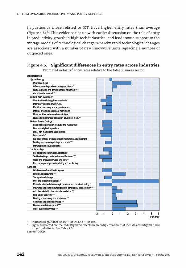
4. FIRM DYNAMICS, PRODUCTIVITY AND POLICY SETTINGS
in particular those related to ICT, have higher entry rates than average
(Figure 4.6).12 This evidence ties up with earlier discussion on the role of entryin productivity growth in high-tech industries, and lends some support to thevintage models of technological change, whereby rapid technological changesare associated with a number of new innovative units replacing a number ofoutpaced ones.
Figure 4.6. Significant differences in entry rates across industriesEstimated industry1 entry rates relative to the total business sector
* indicates signifiance at 1%; ** at 5% and *** at 10%.1. Figures reported are the industry fixed-effects in an entry equation that includes country, size and
time fixed effects. See Table 4.5.Source: OECD.
-2 -1 0 1 2 3 4 5 6
Manufacturing High technology Pharmaceuticals ** Office accounting and computing machinery *** Radio television and communication equipment *** Aircraft and spacecraft ** Medium, High technology Chemicals excluding pharmaceuticals Machinery and equipment n.e.c. Electrical machinery and apparatus n.e.c. Medical precision and optical instruments Motor vehicles trailers and semi-trailers Railroad equipment and transport equipment n.e.c. ** Medium, Low technology Coke refined petroleum products and nuclear fuel Rubber and plastics products Other non-metallic mineral products Basic metals * Fabricated metal products except machinery and equipment Building and repairing of ships and boats *** Manufacturing n.e.c.; recycling Low technology Food products beverages and tobacco Textiles textile products leather and footwear *** Wood and products of wood and cork ** Pulp paper paper products printing and publishingServices Wholesale and retail trade; repairs Hotels and restaurants *** Transport and storage Post and telecommunications *** Financial intermediation except insurance and pension funding ** Insurance and pension funding except compulsory social security *** Activities related to financial intermediation *** Real estate activities *** Renting of machinery and equipment *** Computer and related activities *** Research and development *** Other business activities ***
Per cent-2 -1 0 1 2 3 4 5 6
Manufacturing High technology Pharmaceuticals ** Office accounting and computing machinery *** Radio television and communication equipment *** Aircraft and spacecraft ** Medium, High technology Chemicals excluding pharmaceuticals Machinery and equipment n.e.c. Electrical machinery and apparatus n.e.c. Medical precision and optical instruments Motor vehicles trailers and semi-trailers Railroad equipment and transport equipment n.e.c. ** Medium, Low technology Coke refined petroleum products and nuclear fuel Rubber and plastics products Other non-metallic mineral products Basic metals * Fabricated metal products except machinery and equipment Building and repairing of ships and boats *** Manufacturing n.e.c.; recycling Low technology Food products beverages and tobacco Textiles textile products leather and footwear *** Wood and products of wood and cork ** Pulp paper paper products printing and publishingServices Wholesale and retail trade; repairs Hotels and restaurants *** Transport and storage Post and telecommunications *** Financial intermediation except insurance and pension funding ** Insurance and pension funding except compulsory social security *** Activities related to financial intermediation *** Real estate activities *** Renting of machinery and equipment *** Computer and related activities *** Research and development *** Other business activities ***
Per cent
142 THE SOURCES OF ECONOMIC GROWTH IN THE OECD COUNTRIES – ISBN 92-64-19945-4 – © OECD 2003
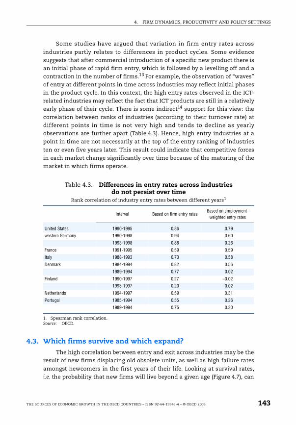
4. FIRM DYNAMICS, PRODUCTIVITY AND POLICY SETTINGS
Some studies have argued that variation in firm entry rates across
industries partly relates to differences in product cycles. Some evidencesuggests that after commercial introduction of a specific new product there isan initial phase of rapid firm entry, which is followed by a levelling off and acontraction in the number of firms.13 For example, the observation of “waves”of entry at different points in time across industries may reflect initial phasesin the product cycle. In this context, the high entry rates observed in the ICT-related industries may reflect the fact that ICT products are still in a relativelyearly phase of their cycle. There is some indirect14 support for this view: thecorrelation between ranks of industries (according to their turnover rate) atdifferent points in time is not very high and tends to decline as yearlyobservations are further apart (Table 4.3). Hence, high entry industries at apoint in time are not necessarily at the top of the entry ranking of industries
ten or even five years later. This result could indicate that competitive forcesin each market change significantly over time because of the maturing of themarket in which firms operate.
Table 4.3. Differences in entry rates across industries do not persist over time
Rank correlation of industry entry rates between different years1
1. Spearman rank correlation.Source: OECD.
4.3. Which firms survive and which expand?
The high correlation between entry and exit across industries may be theresult of new firms displacing old obsolete units, as well as high failure rates
amongst newcomers in the first years of their life. Looking at survival rates,i.e. the probability that new firms will live beyond a given age (Figure 4.7), can
Interval Based on firm entry ratesBased on employment-
weighted entry rates
United States 1990-1995 0.86 0.79
western Germany 1990-1998 0.94 0.60
1993-1998 0.88 0.26
France 1991-1995 0.59 0.59
Italy 1988-1993 0.73 0.58
Denmark 1984-1994 0.82 0.56
1989-1994 0.77 0.02
Finland 1990-1997 0.27 –0.02
1993-1997 0.20 –0.02
Netherlands 1994-1997 0.59 0.31
Portugal 1985-1994 0.55 0.36
1989-1994 0.75 0.30
THE SOURCES OF ECONOMIC GROWTH IN THE OECD COUNTRIES – ISBN 92-64-19945-4 – © OECD 2003 143
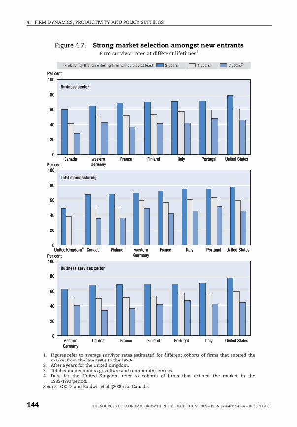
4. FIRM DYNAMICS, PRODUCTIVITY AND POLICY SETTINGS
Figure 4.7. Strong market selection amongst new entrantsFirm survivor rates at different lifetimes1
1. Figures refer to average survivor rates estimated for different cohorts of firms that entered themarket from the late 1980s to the 1990s.
2. After 6 years for the United Kingdom.3. Total economy minus agriculture and community services.4. Data for the United Kingdom refer to cohorts of firms that entered the market in the
1985-1990 period.Source: OECD, and Baldwin et al. (2000) for Canada.
100
80
60
40
20
0
100
80
60
40
20
0
100
80
60
40
20
0
Per centCanada western
GermanyFrance Finland Italy Portugal United States
westernGermany
Canada France Finland Portugal Italy United States
United Kingdom4 Canada westernGermany
FranceFinland Italy Portugal United StatesPer cent
Probability that an entering firm will survive at least: 2 years 4 years 7 years2
Per cent
Business sector3
Total manufacturing
Business services sector
100
80
60
40
20
0
100
80
60
40
20
0
100
80
60
40
20
0
Per centCanada western
GermanyFrance Finland Italy Portugal United States
westernGermany
Canada France Finland Portugal Italy United States
United Kingdom4 Canada westernGermany
FranceFinland Italy Portugal United StatesPer cent
Probability that an entering firm will survive at least: 2 years 4 years 7 years2
Per cent
Business sector3
Total manufacturing
Business services sector
144 THE SOURCES OF ECONOMIC GROWTH IN THE OECD COUNTRIES – ISBN 92-64-19945-4 – © OECD 2003
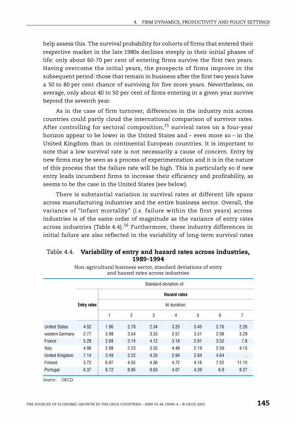
4. FIRM DYNAMICS, PRODUCTIVITY AND POLICY SETTINGS
help assess this. The survival probability for cohorts of firms that entered their
respective market in the late 1980s declines steeply in their initial phases oflife: only about 60-70 per cent of entering firms survive the first two years.Having overcome the initial years, the prospects of firms improve in thesubsequent period: those that remain in business after the first two years havea 50 to 80 per cent chance of surviving for five more years. Nevertheless, onaverage, only about 40 to 50 per cent of firms entering in a given year survivebeyond the seventh year.
As in the case of firm turnover, differences in the industry mix acrosscountries could partly cloud the international comparison of survivor rates.After controlling for sectoral composition,15 survival rates on a four-yearhorizon appear to be lower in the United States and – even more so – in theUnited Kingdom than in continental European countries. It is important tonote that a low survival rate is not necessarily a cause of concern. Entry bynew firms may be seen as a process of experimentation and it is in the natureof this process that the failure rate will be high. This is particularly so if newentry leads incumbent firms to increase their efficiency and profitability, asseems to be the case in the United States (see below).
There is substantial variation in survival rates at different life spansacross manufacturing industries and the entire business sector. Overall, thevariance of “infant mortality” (i.e. failure within the first years) acrossindustries is of the same order of magnitude as the variance of entry ratesacross industries (Table 4.4).16 Furthermore, these industry differences ininitial failure are also reflected in the variability of long-term survival rates
Table 4.4. Variability of entry and hazard rates across industries, 1989-1994
Non-agricultural business sector, standard deviations of entry and hazard rates across industries
Source: OECD.
Standard deviation of:
Entry rates
Hazard rates
At duration:
1 2 3 4 5 6 7
United States 4.52 1.96 2.78 2.34 3.25 3.45 2.76 2.26
western Germany 2.77 3.98 3.54 3.53 2.57 3.51 2.08 3.29
France 5.29 2.68 3.14 4.12 3.18 2.91 3.52 7.8
Italy 4.98 2.99 2.23 3.33 4.48 2.19 2.59 4.15
United Kingdom 7.14 3.49 3.22 4.33 2.94 2.84 4.64 . .
Finland 3.72 6.97 4.55 4.36 4.72 4.16 7.52 11.15
Portugal 6.37 8.72 8.95 9.63 4.07 4.39 6.9 8.27
THE SOURCES OF ECONOMIC GROWTH IN THE OECD COUNTRIES – ISBN 92-64-19945-4 – © OECD 2003 145
4. FIRM DYNAMICS, PRODUCTIVITY AND POLICY SETTINGS
(i.e. five-seven years of age), which remains substantial. To the extent that
cross-industry variability may be taken as an indicator of the different marketbarriers that affect young firms, the evidence reported in Table 4.4 mayindicate a degree of commonality between industry characteristics that affectbarriers to entry and those that condition firm survival.17
The process of entry and exit of firms involves a proportionally lownumber of workers, i.e. employment turnover related to the process of entry
and exit is lower than firm turnover, because entrants and exiting firms aregenerally smaller than incumbents (Figure 4.8, and Box 4.4). The particularlysmall size of entrants in the United States, Canada and Germany reflectseither the large size of incumbents (e.g. the United States, see Bartelsman et
al., 2002) or the small average size of entrants compared with that in mostother countries (Germany and Canada, see Figure 4.8). In other words, entrantfirms are further away from the average size in these countries. At the sametime, there is general tendency for failure in the early years of activity to beconcentrated amongst small units, while surviving firms are not only largerbut also tend to grow rapidly. Thus, in most countries the size of exiting firmsis broadly similar to that of entering firms. Moreover, the average size ofsurviving firms increases rapidly to approach that of incumbents in the
market in which they operate. However, the expansion of surviving firms isnotably higher in the United States than in Europe (Figure 4.9).18
The marked difference in post-entry behaviour of firms in the UnitedStates, compared with European countries, is partially due to the larger gapbetween the size at entry and the average firm size of incumbents, i.e. there is
a greater scope for expansion amongst young ventures in the US markets thanin Europe. In turn, the smaller relative size of entrants can be taken to indicatea greater degree of experimentation, with firms starting small and, ifsuccessful, expanding rapidly to approach the minimum efficient scale.19 Firmcharacteristics at entry are influenced by market conditions (concentration,product diversification, advertising costs, etc.) but may also depend onregulations and institutions affecting start-up costs and efficiency-enhancingdecisions by existing firms, as discussed below.
4.4. Regulations, institutions and firm entry: empirical analysis
This section aims at exploring possible policy and institutional influenceson the observed patterns of firm entry documented earlier. Its main objectiveis to assess whether policy factors help explain the observed differences inentry rates across countries and industries, by linking together the firm-leveldataset described above with the OECD indicators of regulations andinstitutional settings already used in Chapter 3 above. The limits inherent tothis empirical methodology are very similar to – and arguably more significant
146 THE SOURCES OF ECONOMIC GROWTH IN THE OECD COUNTRIES – ISBN 92-64-19945-4 – © OECD 2003
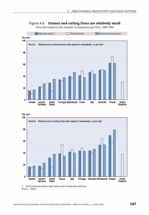
4. FIRM DYNAMICS, PRODUCTIVITY AND POLICY SETTINGS
Figure 4.8. Entrant and exiting firms are relatively smallFirm size based on the number of employees per firm, 1989-1994
1. Total economy minus agriculture and community services.Source: OECD.
100
80
60
40
20
0
100
80
60
40
20
0Netherlandswestern
GermanyItaly FinlandFrance DenmarkPortugalCanada United
StatesUnited
Kingdom
Italy DenmarkwesternGermany
Finland UnitedKingdom
NetherlandsCanada FranceUnitedStates
Portugal
Per cent
Panel A. Relative size of entering firms with respect to incumbents, in per cent
Business sector1 Manufacturing Business service sector
Per cent
Panel B. Relative size of exiting firms with respect to incumbents, in per cent
100
80
60
40
20
0
100
80
60
40
20
0Netherlandswestern
GermanyItaly FinlandFrance DenmarkPortugalCanada United
StatesUnited
Kingdom
Italy DenmarkwesternGermany
Finland UnitedKingdom
NetherlandsCanada FranceUnitedStates
Portugal
Per cent
Panel A. Relative size of entering firms with respect to incumbents, in per cent
Business sector1 Manufacturing Business service sector
Per cent
Panel B. Relative size of exiting firms with respect to incumbents, in per cent
THE SOURCES OF ECONOMIC GROWTH IN THE OECD COUNTRIES – ISBN 92-64-19945-4 – © OECD 2003 147
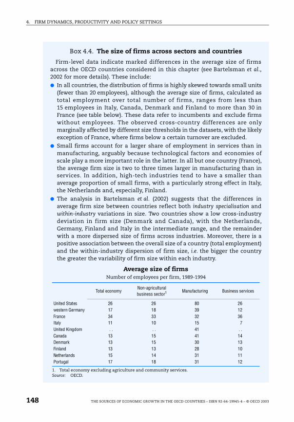
4. FIRM DYNAMICS, PRODUCTIVITY AND POLICY SETTINGS
s.,
ss
syy
f),
,
y,ra)y
Box 4.4. The size of firms across sectors and countries
Firm-level data indicate marked differences in the average size of firmacross the OECD countries considered in this chapter (see Bartelsman et al2002 for more details). These include:
In all countries, the distribution of firms is highly skewed towards small unit(fewer than 20 employees), although the average size of firms, calculated atotal employment over total number of firms, ranges from less than15 employees in Italy, Canada, Denmark and Finland to more than 30 inFrance (see table below). These data refer to incumbents and exclude firmwithout employees. The observed cross-country differences are onlmarginally affected by different size thresholds in the datasets, with the likelexception of France, where firms below a certain turnover are excluded.
Small firms account for a larger share of employment in services than inmanufacturing, arguably because technological factors and economies oscale play a more important role in the latter. In all but one country (Francethe average firm size is two to three times larger in manufacturing than inservices. In addition, high-tech industries tend to have a smaller thanaverage proportion of small firms, with a particularly strong effect in Italythe Netherlands and, especially, Finland.
The analysis in Bartelsman et al. (2002) suggests that the differences inaverage firm size between countries reflect both industry specialisation andwithin-industry variations in size. Two countries show a low cross-industrdeviation in firm size (Denmark and Canada), with the NetherlandsGermany, Finland and Italy in the intermediate range, and the remaindewith a more dispersed size of firms across industries. Moreover, there is positive association between the overall size of a country (total employmentand the within-industry dispersion of firm size, i.e. the bigger the countrthe greater the variability of firm size within each industry.
Average size of firmsNumber of employees per firm, 1989-1994
1. Total economy excluding agriculture and community services.Source: OECD.
Total economyNon-agriculturalbusiness sector1 Manufacturing Business services
United States 26 26 80 26western Germany 17 18 39 12France 34 33 32 36Italy 11 10 15 7United Kingdom . . . . 41 . .Canada 13 15 41 14Denmark 13 15 30 13Finland 13 13 28 10Netherlands 15 14 31 11Portugal 17 18 31 12
148 THE SOURCES OF ECONOMIC GROWTH IN THE OECD COUNTRIES – ISBN 92-64-19945-4 – © OECD 2003
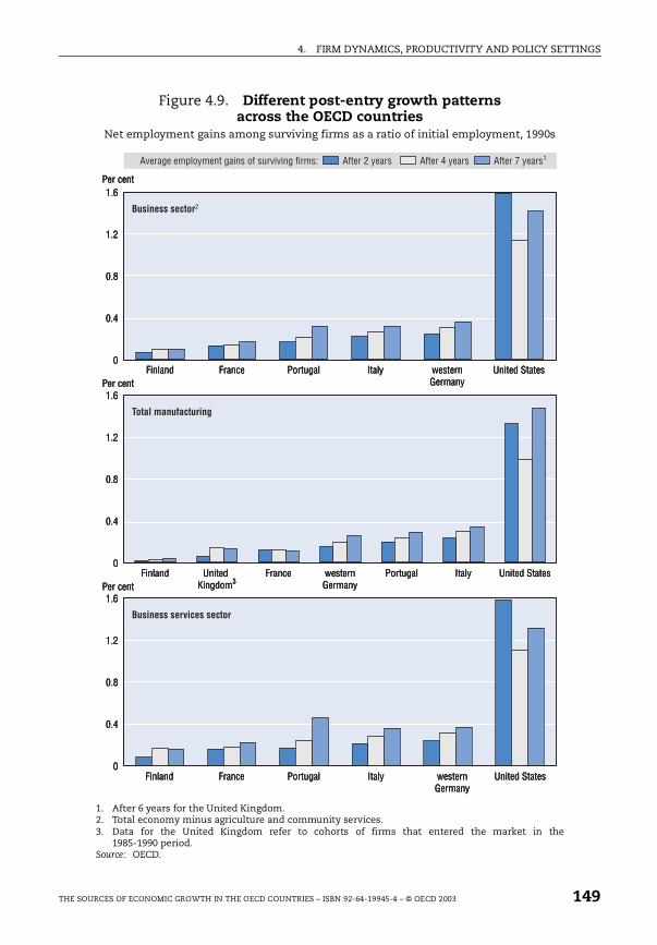
4. FIRM DYNAMICS, PRODUCTIVITY AND POLICY SETTINGS
Figure 4.9. Different post-entry growth patterns across the OECD countries
Net employment gains among surviving firms as a ratio of initial employment, 1990s
1. After 6 years for the United Kingdom.2. Total economy minus agriculture and community services.3. Data for the United Kingdom refer to cohorts of firms that entered the market in the
1985-1990 period.Source: OECD.
1.6
1.2
0.8
0.4
0
1.6
1.2
0.8
0.4
0
1.6
1.2
0.8
0.4
0
Per centwesternGermany
FranceFinland ItalyPortugal United States
westernGermany
FranceFinland Portugal United States
United Kingdom3
westernGermany
FranceFinland Italy
Italy
Portugal United StatesPer cent
Average employment gains of surviving firms: After 2 years After 4 years After 7 years1
Per cent
Business sector2
Total manufacturing
Business services sector
1.6
1.2
0.8
0.4
0
1.6
1.2
0.8
0.4
0
1.6
1.2
0.8
0.4
0
Per centwesternGermany
FranceFinland ItalyPortugal United States
westernGermany
FranceFinland Portugal United States
United Kingdom3
westernGermany
FranceFinland Italy
Italy
Portugal United StatesPer cent
Average employment gains of surviving firms: After 2 years After 4 years After 7 years1
Per cent
Business sector2
Total manufacturing
Business services sector
THE SOURCES OF ECONOMIC GROWTH IN THE OECD COUNTRIES – ISBN 92-64-19945-4 – © OECD 2003 149
4. FIRM DYNAMICS, PRODUCTIVITY AND POLICY SETTINGS
than – those mentioned in Chapter 3: most importantly, the decision of a firm
to enter the market depends on a number of additional factors that are notcontrolled for. In addition, the country coverage is relatively narrow.Therefore, the evidence presented in this section and its policy implicationsshould be viewed as tentative.
The entry equation is based on a theoretical model in which entrydepends on the expected (post-entry) profits, defined net of the costs of
entry.20 In the estimates, the actual proxies for these two variables are thesmoothed growth rate of industry value-added for market profitability, andthe smoothed capital intensity (i.e. capital stock divided by value added) forentry costs: high capital intensity implies a large share of fixed costs and thusraises entry costs, ceteris paribus. In this framework, indicators of thestringency of regulations can also influence entrepreneurship. The analysisalso accounts for the size effect on firm dynamics (using five size classes, fromfewer than 20 employees to more than 500 employees), and allows testingwhether incentives and disincentives to entry differ according to the size offirms.
Table 4.5 presents the baseline entry equation, which neither controls forthe impact of net expected profits nor for the effect of policy and institutionalfactors. The results only shed some light on possible country and size effectson entry rates, once control for sector composition is taken into account.Equation A includes year dummies to control for specific time effects, whileEquation B uses a country-specific measure of the business cycle. Equation Cincludes both, in order to test for common and country-specific time patterns
of entry. Since the inclusion of the business cycle variable in a specificationwith time dummies does not significantly affect the results, it is not includedin the other specifications. Equation D controls for the presence of outliers inthe data and Equation E replicates it without size dummies to identify theoverall country-specific effects, including those related to differences in thesize structure of firms. As noted in Section 4.2, the estimated countrydifferences in entry rates are generally statistically significant, but not verylarge, once control is made for the industry composition of the economy.Moreover, with the exception of Germany and Italy, entry rates are higher inthe United States (the reference country in all regressions) than in othercountries, ceteris paribus. The results also suggest a non-linear relationshipbetween the entry rates and size: small firms (with fewer than 20 employees)
have significantly higher entry rates than the reference group (20-49), whilelarger firms (50 and more) have only marginally lower entry rates with respectto the reference group.
Table 4.6 moves one step further in the analysis to include proxies forprofitability and entry barriers that could partially account for the country(and industry) fixed effects. The analysis starts with the most parsimonious
150 THE SOURCES OF ECONOMIC GROWTH IN THE OECD COUNTRIES – ISBN 92-64-19945-4 – © OECD 2003
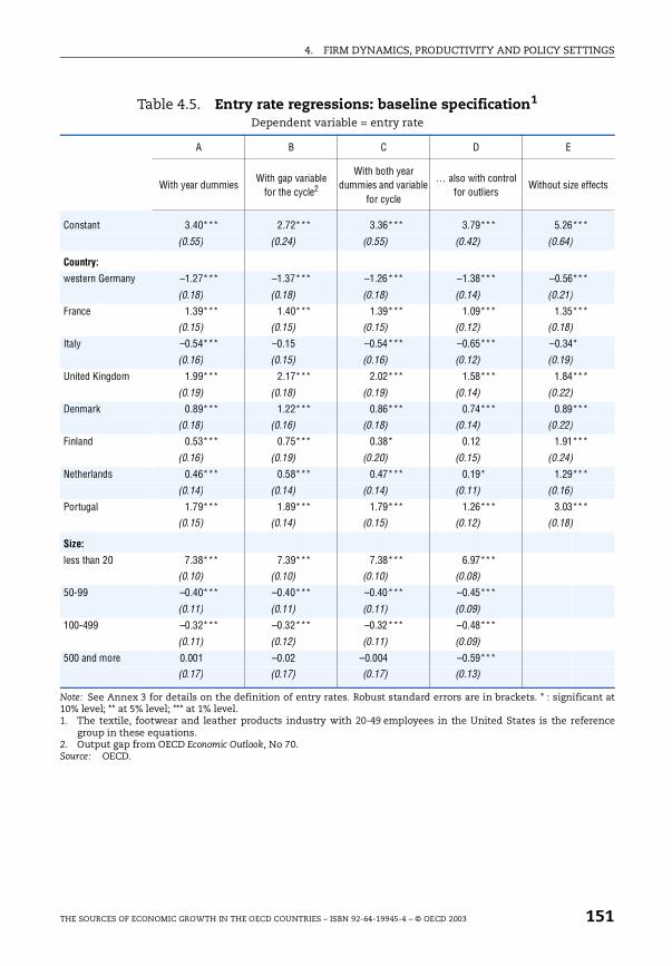
4. FIRM DYNAMICS, PRODUCTIVITY AND POLICY SETTINGS
nt at
ence
ects
Table 4.5. Entry rate regressions: baseline specification1
Dependent variable = entry rate
Note: See Annex 3 for details on the definition of entry rates. Robust standard errors are in brackets. * : significa10% level; ** at 5% level; *** at 1% level.1. The textile, footwear and leather products industry with 20-49 employees in the United States is the refer
group in these equations.2. Output gap from OECD Economic Outlook, No 70.Source: OECD.
A B C D E
With year dummiesWith gap variable
for the cycle2
With both year dummies and variable
for cycle
… also with control for outliers
Without size eff
Constant 3.40*** 2.72*** 3.36*** 3.79*** 5.26***
(0.55) (0.24) (0.55) (0.42) (0.64)
Country:
western Germany –1.27*** –1.37*** –1.26*** –1.38*** –0.56***
(0.18) (0.18) (0.18) (0.14) (0.21)
France 1.39*** 1.40*** 1.39*** 1.09*** 1.35***
(0.15) (0.15) (0.15) (0.12) (0.18)
Italy –0.54*** –0.15 –0.54*** –0.65*** –0.34*
(0.16) (0.15) (0.16) (0.12) (0.19)
United Kingdom 1.99*** 2.17*** 2.02*** 1.58*** 1.84***
(0.19) (0.18) (0.19) (0.14) (0.22)
Denmark 0.89*** 1.22*** 0.86*** 0.74*** 0.89***
(0.18) (0.16) (0.18) (0.14) (0.22)
Finland 0.53*** 0.75*** 0.38* 0.12 1.91***
(0.16) (0.19) (0.20) (0.15) (0.24)
Netherlands 0.46*** 0.58*** 0.47*** 0.19* 1.29***
(0.14) (0.14) (0.14) (0.11) (0.16)
Portugal 1.79*** 1.89*** 1.79*** 1.26*** 3.03***
(0.15) (0.14) (0.15) (0.12) (0.18)
Size:
less than 20 7.38*** 7.39*** 7.38*** 6.97***
(0.10) (0.10) (0.10) (0.08)
50-99 –0.40*** –0.40*** –0.40*** –0.45***
(0.11) (0.11) (0.11) (0.09)
100-499 –0.32*** –0.32*** –0.32*** –0.48***
(0.11) (0.12) (0.11) (0.09)
500 and more 0.001 –0.02 –0.004 –0.59***
(0.17) (0.17) (0.17) (0.13)
THE SOURCES OF ECONOMIC GROWTH IN THE OECD COUNTRIES – ISBN 92-64-19945-4 – © OECD 2003 151
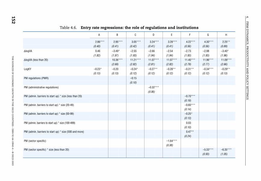
4.FIR
M D
YN
AM
ICS
, PRO
DU
CT
IVIT
Y A
ND
POLIC
Y SET
TIN
GS
152T
HE S
OU
RC
ES O
F EC
ON
OM
IC G
RO
WT
H IN
TH
E OEC
D C
OU
NT
RIES – ISB
N 92-64-19945-4 – ©
OEC
D 2003
ons and institutions
E F G H
3.28*** 4.22*** 4.30*** 2.25**
(0.41) (0.56) (0.56) (0.89)
–2.54 –2.73 –2.98 –3.40*
(1.94) (1.93) (1.93) (1.96)
11.07*** 11.40*** 11.96*** 11.09***
(2.82) (2.79) (2.77) (2.66)
–0.28** –0.31** –0.34*** –0.29**
(0.12) (0.12) (0.12) (0.13)
–0.70***
(0.19)
–0.60***
(0.14)
–0.25*
(0.13)
0.03
(0.10)
0.47**
(0.24)
–1.64***
(0.38)
–5.33*** –6.35***
(0.93) (1.05)
Table 4.6. Entry rate regressions: the role of regulati
A B C D
2.86*** 2.95*** 3.05*** 3.24***
(0.40) (0.41) (0.42) (0.41)
∆logVA 0.46 –3.49* –2.55 –2.66
(1.82) (1.97) (1.93) (1.94)
∆logVA (less than 20) 10.36*** 11.21*** 11.07***
(2.69) (2.82) (2.81)
LogKY –0.23* –0.20 –0.24* –0.27**
(0.13) (0.13) (0.12) (0.12)
PM regulations (PMR) –0.15
(0.10)
PM (administrative regulations) –0.32***
(0.06)
PM (admin. barriers to start up) * size (less than 20)
PM (admin. barriers to start up) * size (20-49)
PM (admin. barriers to start up) * size (50-99)
PM (admin. barriers to start up) * size (100-499)
PM (admin. barriers to start up) * size (500 and more)
PM (sector specific)
PM (sector specific) * size (less than 20)
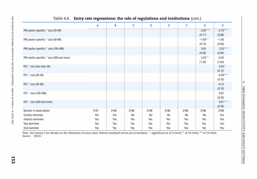
4.FIR
M D
YN
AM
ICS, PR
OD
UC
TIV
ITY
AN
D PO
LICY
SETT
ING
S
TH
E SOU
RC
ES OF EC
ON
OM
IC G
RO
WT
H IN
TH
E OEC
D C
OU
NT
RIES
– ISB
N 92-64-19945-4 – ©
OE
CD
2003153
Table 4.6. Entry rate regressions: the role of regulations and institutions (cont.)
ficant at 10 % level; ** at 5% level; *** at 1% level.
E F G H
–3.95*** –2.70***
(0.77) (0.96)
–1.65** –1.05
(0.75) (0.93)
0.83 2.53***
(0.58) (0.94)
3.25** –2.32
(1.35) (1.94)
0.23*
(0.12)
–0.28***
(0.10)
–0.13
(0.10)
0.07
(0.34)
0.87***
(0.20)
3196 3198 3198 3196
No No No Yes
Yes Yes Yes Yes
Yes Yes Yes Yes
Yes Yes Yes Yes
Note: See Annex 3 for details on the definition of entry rates. Robust standard errors are in brackets. * : signiSource: OECD.
A B C D
PM (sector specific) * size (20-49)
PM (sector specific) * size (50-99)
PM (sector specific) * size (100-499)
PM (sector specific) * size (500 and more)
EPL * size (less than 20)
EPL * size (20-49)
EPL * size (50-99)
EPL * size (100-499)
EPL * size (500 and more)
Number of observations 3197 3196 3196 3196
Country dummies Yes Yes No No
Industry dummies Yes Yes Yes Yes
Year dummies Yes Yes Yes Yes
Size dummies Yes Yes Yes Yes
4. FIRM DYNAMICS, PRODUCTIVITY AND POLICY SETTINGS
specification, then adds other explanatory variables, and ends with the most
comprehensive equation (Equation H), offering the best statistical fit. Theresults are largely as expected:
The growth rate of industry value-added has a positive impact on entry.There is also evidence of a significantly larger effect for small rather thanother firms, so that a distinction is considered from Equation B onwards.
Costs of entry, as proxied by capital intensity, appear to negatively affectentry rates (though at somewhat variable levels of significance).
In most cases, the stringency of product market regulations also significantlylowers entries. Administrative regulations on entrepreneurial activities seemto be particularly detrimental to entry (column D). This negative effect is feltby small- and medium-sized firms, while on the contrary it is found to bepositive for larger firms (column F). All these findings appear to be relativelyrobust to the choice of the PMR indicator (columns E and G).21 The positiveeffect of regulation on the entry of large firms is puzzling, but it is likely to beinfluenced by the characteristics of such firms in the sample: there areindeed few of them and some large entries are the result of mergers.
There is a negative impact on entry of the strictness of employmentprotection legislation.22 At first glance this effect seems to be complex(Equation H): tight regulations on hiring and firing appear to increaseentries of micro firms, while lowering those of small/medium-sized ones,ceteris paribus. However, this finding is consistent with the fact that in anumber of countries with relatively tight EPL (e.g. Germany, Italy, Portugal),firms below a given size threshold (ranging from 5 to 25 employees) are
exempted from certain aspects of the employment protection legislation.23
Under these circumstances, firm entry seems to shift towards eithersmaller units – partially exempted from EPL – or to significantly larger ones,for which hiring and firing costs play a smaller role in total expected entrycosts, as well as in the subsequent costs of adjusting the workforce.24
In summary, taken at face value these results suggest a statistically
significant (albeit not large) direct effect of regulation on entry rates. Inparticular, a reduction in the administrative barriers to entrepreneurialactivity equal to two standard deviations (calculated on the basis of the cross-country distribution) could lead to an increase in entry rates amongst smallfirms by about 1.3 percentage points (around 10 per cent of the cross-countryaverage in entry rates). An easing of employment protection legislation of thesame magnitude could raise entry rates amongst small- and medium-sizedfirms by about 0.7 percentage points. These are direct effects, to which may beadded possible indirect effects stemming from the impact of these regulatoryreforms on productivity and, possibly, on the size distribution of firms(see Nicoletti et al., 2001).
154 THE SOURCES OF ECONOMIC GROWTH IN THE OECD COUNTRIES – ISBN 92-64-19945-4 – © OECD 2003
4. FIRM DYNAMICS, PRODUCTIVITY AND POLICY SETTINGS
4.5. Concluding remarks
A key finding of the firm-level analysis presented in this chapter is that
over a five-year horizon, aggregate labour productivity growth is mainly drivenby what happens in each individual firm, whilst shifts in market shares fromlow- to high-productivity firms and net entry seem to play only a modest role.However, this conclusion should be qualified on two grounds:
First of all, there is tentative evidence suggesting that within-firm growthmakes a smaller contribution to multi-factor productivity growth than it
does to labour productivity growth. Since multi-factor productivity growthis a proxy for overall efficiency in the production process, this resultsuggests that incumbents often raise labour productivity by increasingcapital intensity and/or shedding labour, while new firms provide arelatively larger contribution to overall efficiency, possibly by entering themarket with a more “efficient” mix of capital and labour and likely newtechnologies.
More importantly, even in terms of labour (rather than multi-factor)productivity, there are some industries where the entry of new unitssignificantly boosts industry-wide growth. This is clearly the case for high-tech industries, where new firms are more likely to adopt state-of-the-arttechnologies. Interestingly, the United States, the country at the forefront inadopting new technologies over the recent period,has also displayed greatervariability of productivity levels amongst entering firms than othercountries for which the data was available.
The analysis of firm dynamics presented in this chapter points to asignificant and broadly similar degree of “firm churning” amongst OECDcountries. More specifically, the high correlation between entry and exit ratesacross industries suggests a process of “creative destruction” in which a largenumber of new firms displace a large number of inefficient firms. This doesnot prevent the likelihood of failure of entrants from being high, especially forsmall firms, which suggests that “creative destruction” also involves a greatdeal of market experimentation. However, surviving firms tend to growrapidly towards the average (efficient) size.
Both European and US firms share these general features, but to asomewhat different extent. US entrant firms appear to be smaller and lessproductive than their European counterparts, but grow faster whensuccessful. The econometric results presented in this chapter offer somerationale for these differences. Indeed, they support the view that strictregulations on entrepreneurial activity, as well as high costs of adjusting the
workforce negatively affect the entry of new (especially small) firms. Thus, inthe United States, low administrative costs of start-ups, and not unduly strictregulations on labour adjustments, are likely to stimulate potential
THE SOURCES OF ECONOMIC GROWTH IN THE OECD COUNTRIES – ISBN 92-64-19945-4 – © OECD 2003 155
4. FIRM DYNAMICS, PRODUCTIVITY AND POLICY SETTINGS
entrepreneurs to start on a small scale, test the market and, if successful with
their business plan, expand rapidly to reach the minimum efficient scale. Incontrast, higher entry and adjustment costs in Europe may stimulate a pre-market selection of business plans with less market experimentation. Inaddition, the more market-based financial system may lead to a lower riskaversion to project financing in the United States, with greater financingpossibilities for entrepreneurs with small or innovative projects, oftencharacterised by limited cash flows and lack of collateral.
There is no evidence in the available data that one model dominates theother in terms of aggregate performance. However, in a period (like thepresent) of rapid diffusion of a new technology (ICT), greater experimentationmay allow new ideas and forms of production to emerge more rapidly, therebyleading to a faster process of innovation and technology adoption. This seemsto be confirmed by the strong contribution to overall productivity made bynew firms in ICT-related industries over the recent period (see Chapter 3above). In this context, easing regulations may stimulate firm entry and, via
this channel, may ultimately lead to higher productivity growth.
Notes
1. It would, however, have been somewhat larger had the decomposition followedthe approach proposed by Foster et al. (1998) (see Scarpetta et al. (2002) for moredetails). Their methodology uses base-year market shares as weights for eachterm of the decomposition, and includes an additional term (the so-called“covariance” or “cross” term) that combines changes in market shares andchanges in productivity. This term is positive if enterprises with growingproductivity also experience an increase in market share, and negative otherwise.When labour productivity growth in manufacturing was decomposed along theselines, the “cross” term appeared to be negative, implying that firms experiencingan increase in productivity were also losing market shares, i.e. their productivitygrowth was associated with restructuring and downsizing rather than expansion.Under these circumstances, the overall contribution to GDP growth of these firmsis lower than that for labour productivity and may even be negative.
2. These results are broadly consistent with findings in Baily et al. (1992) andHaltiwanger (1997).
3. For France and Italy, the data are somewhat problematic in the context of aninternational comparison, and should, therefore, be interpreted with great care.The French data refer to firms with at least 20 employees or with a turnovergreater than EUR 0.58 m, which are not likely to be representative of the totalpopulation. In addition, larger firms may be over-sampled, lowering the net entryeffect and raising the within effect. The Italian data refer to firms with a turnoverof at least EUR 5 m, and sample size is maintained by deleting firms falling belowthe threshold and adding new firms in. Thus, the Italian data are likely tooverstate true entry and exit rates. Furthermore, the sampling rules are likely toover-record exiting firms with falling productivity (see Scarpetta et al., 2002).
4. The share of activity (the weighting factor in the decomposition, see Box 3.3) ofentrants in the end year increases with the horizon over which the end year ismeasured (see Foster et al., 1998).
156 THE SOURCES OF ECONOMIC GROWTH IN THE OECD COUNTRIES – ISBN 92-64-19945-4 – © OECD 2003

4. FIRM DYNAMICS, PRODUCTIVITY AND POLICY SETTINGS
5. See Baily et al. (1996, 1997) and Haltiwanger (1997).
6. The industry group is “electrical and optical equipment”. In the United States, most3-4 digit industries within this group had a positive contribution to productivitystemming from entry. In the other countries, there are cases where, within thisgroup, the contribution from entry is very high, including the “office, accounting andcomputing machinery” industry in Finland, the United Kingdom and Portugal and“precision instruments” in France, Italy and the Netherlands.
7. In particular, Chapter 1 has shown that in many continental European countrieshigh labour productivity growth in the 1990s was accompanied by significant fallsin employment, especially in manufacturing. Moreover, the relatively high labourproductivity growth was accompanied by significant falls in MFP growth withrespect to the previous decade.
8. See e.g. Geroski (1991), Baldwin and Gorecki (1991).
9. The values reported in the Figure 4.5 are the estimated country-specific effects ofa panel regression of entry rates on a set of dummy variables accounting forindustry, country and time effects.
10. Indeed, the different size structure of firms across countries is not included in thecountry fixed effects of the panel data regression.
11. The lower turnover rate in the French service sector, compared with that inmanufacturing, is likely to depend on the existence of a size threshold in theFrench data (see Scarpetta et al., 2002), which tends to be more binding in theservice sector than in manufacturing. As an indication, the French data alsosuggest a higher average size of firms in the service sector than in manufacturing,in contrast with all other countries.
12. The very high positive effect for the post and telecommunication industry is likely tobe due to two factors: i) the privatisation of telecommunications in a number ofcountries which has led to the entry of a number of new private operators; andii) the rapid increase in the number of firms operating in the communicationsarea, related to the spread of Internet and e-commerce activities.
13. For example, a study of 46 products in the United States by Gort and Klepper (1982)found a typical initial phase of entry of about 10 years and a phase of contractionof about 5 years.
14. Following specific products over time would have led to more direct evidence, butin the context of this book such data were not available.
15. The corresponding results are not reported here. See Scarpetta et al. (2002).
16. In Table 4.4, hazard rates at duration i are the estimated probabilities of exiting themarket conditional on having survived for at least i years.
17. See also Geroski (1995) and Audretsch and Mahmood (1994).
18. The results for the United States are consistent with the evidence in Audretsch(1995).
19. There is also a greater variability of productivity levels amongst entering in theUnited States compared with European countries, which is also consistent withthe idea of greater “experimentation”. However, there are other additional factorsthat could contribute to explain the observed differences in post-entry behaviour,including the larger size of the US market compared to that of EU countries. SeeBartelsman et al., 2002 for details on these factors.
THE SOURCES OF ECONOMIC GROWTH IN THE OECD COUNTRIES – ISBN 92-64-19945-4 – © OECD 2003 157
4. FIRM DYNAMICS, PRODUCTIVITY AND POLICY SETTINGS
20. See Geroski (1995) and Siegfried and Evans (1994) for a survey.
21. Such robustness is reassuring, because the lack of sectoral or time dimensions inthe PMR indicators used in equations C, D and F of Table 4.6 implied that noadditional control for country fixed effects could be included in equations. Thiscould have potentially led to assigning an explanatory power to these regulatoryindicators, which was, in fact, due to other omitted country-specific influences.
22. From an empirical point of view, the inclusion of EPL in the regression isproblematic, given the high correlation with the overall indicator of productmarket regulation. In order to identify the two effects, equation H uses the sector-specific indicator of product market regulation, together with a nation-wide – buttime-varying – indicator of EPL. In other words, the time dimension allowsidentification of the EPL coefficient, the sectoral dimension identifies the productmarket indicator, and the inclusion of country dummies minimises the risk of anomitted variable problem.
23. These results also seem consistent with those presented in Nicoletti et al. (2001)pointing to a negative effect of EPL on the average size of firms.
24. Indeed, the incidence of strict EPL on total labour adjustment costs may declinewith the size of the firm, as larger ones may more easily reallocate labour withinthem and spread these costs over a larger capital stock. Nevertheless, thisargument is insufficient to explain the positive effect of EPL found for very largefirms (500 employees and more). As stressed above in the text, this result shouldnot be overemphasised, insofar as there are a relatively small number ofobservations for this size class across industries and countries.
158 THE SOURCES OF ECONOMIC GROWTH IN THE OECD COUNTRIES – ISBN 92-64-19945-4 – © OECD 2003

ISBN 92-64-19945-4
The Sources of Economic Growth in the OECD Countries© OECD 2003
Annex 1
Macroeconomic indicators of economic growth
A1.1. Measurement of labour and capital inputs
Measures of factor use for the purpose of productivity analysis areconstructed so as to reflect the role that each factor plays as input in theproduction process. In the case of labour input, different types of labourshould be weighted by their marginal contribution to the production activityin which they are employed. Since these productivity measures are generallynot observable, information on relative wages by characteristics is used toderive the required weights to aggregate different types of labour. Concerningphysical capital, Jorgenson (1963) and Jorgenson and Griliches (1967) were thefirst to develop aggregate capital input measures that took the heterogeneityof assets into account. They defined the flow of quantities of capital servicesindividually for each type of asset, and then applied asset-specific user costs
as weights to aggregate across services from the different types of assets. Usercosts are prices for capital services and, under competitive markets andequilibrium conditions, these prices reflect marginal productivity of thedifferent assets. User cost weights are thus a means to effectively incorporatedifferences in the productive contribution of heterogeneous investments asthe composition of investment and capital changes. Changes in aggregatecapital input, therefore, have two distinct sources – changes in the quantity ofcapital of a given type, and changes in the composition of the various types ofassets with different marginal products and user costs (Ho et al., 1999).
Productivity growth measures without adjustment for different types of factor input
The following notation is used to discuss factor productivity with andwithout control for quality effects:
Y Current price value-added;P Price index of value-added;N Total number of persons engaged;H Average hours worked per person;N*H Total hours worked;Κ Aggregate gross capital stock.
THE SOURCES OF ECONOMIC GROWTH IN THE OECD COUNTRIES – ISBN 92-64-19945-4 – © OECD 2003 159
ANNEX 1
Letting lower case letters represent logarithms and ∆ the first difference
operator, ∆x approximates the (instantaneous) growth rate of any variable x.The standard measure of factor productivity growth rates, ∆πL and ∆πK aregiven by:
∆πL=∆y – ∆p – (∆n + ∆h) Labour productivity
∆πK=∆y – ∆p – ∆k Capital productivity
This standard specification does not differentiate between different types
of inputs: it attaches the same weight to each hour worked, and it does notdifferentiate between assets even though their marginal contribution tooutput may be quite different. Such differentiation can be introduced whenthere is information on quantities and prices of the different types of factorinputs. In the case of labour, prices will represent the skill-specific wage rate,and in the case of capital the asset specific rental price or user cost of capital.In what follows different types of labour and capital will be distinguished bythe subscript j.
Productivity growth measures with adjustment for different types of factor input
Given a set of observations on different types of labour or capital anda set of corresponding prices, wj,t it is possible to construct an aggregatevariable F that combines quantities of different types of inputs to a measure oftotal, quality-adjusted labour or capital input. In this regard, productivitystudies often use the Törnqvist index and this practice is followed here. ATörnqvist index of factor input F is given by the expression below, where vj,t
stands for the share of the component j in total costs of the factor. This is aconceptually correct measure for the flow of the total quantity of labour or
capital services:
Thus, the growth rate of total factor input ∆f, using the Törnqvist index,is a weighted average of the growth rates of different components. Weightscorrespond to the current price share in the overall cost for each factor.Subtracting the unadjusted measure of factor input from the one adjusted forcompositional changes yields an expression ∆cf for the effects of changingfactor quality on total factor input services:
∆cl = ∆l(adj) – (∆n + ∆h) [A1.2]
∆ck = ∆k(adj) – ∆k [A1.3]
( ) .2
1)(
,,
,,
,1,,,,, ∑∑ =+=∆⋅=∆ −
i
titi
tjtj
tjtjtjtj
j
tjtjtFw
Fwvandvvvwherefvadjf [A1.1]
160 THE SOURCES OF ECONOMIC GROWTH IN THE OECD COUNTRIES – ISBN 92-64-19945-4 – © OECD 2003
ANNEX 1
Equations [A1.2] and [A1.3] can be rearranged to yield a decomposition of
the overall growth in factor input:
∆l(adj) = ∆cl + ∆n + ∆h
∆k(adj) = ∆ck + ∆k
Labour input
In order to consider changes in the composition of labour input, six
different types of labour were considered, based on gender and three differenteducational levels: below upper secondary education; upper secondaryeducation and tertiary education. Thus, following equation A1.1 andassuming that Lj indicates the labour input jth with j = 1, 2, ..6 and that eachtype of labour is remunerated with wage rate wj, then a measure of adjustedlabour input can be obtained. There are, however, a number of issues worthnoting, including:
First, it is assumed that the rate change in average weekly or yearly hours isidentical between education and gender groups, i.e. ∆h,j = ∆h for all j. Thissimplification can be used, in conjunction with the relation ∆l,j = ∆n,j + ∆h,j.
Second, data on relative wage rates by educational attainment and gender areonly available for the 1990s, and relative wage rates were thus assumed to
be constant over the period considered in the analysis. More specifically, forthe six available categories of education and gender, the wage spread was
computed as , j = 2, 3, 4, 5, 6 as each education category’s wage rate
relative to wages of male workers with upper-secondary education(wM,U-SE).
The weights vj,c from equation [A1.1] for country c can be rewritten in termsof relative wages:
Capital input1
Standard measures of capital (based on aggregation of stocks made up ofa moving sum of investment at real acquisition prices) rely on twoassumptions: 1) the flow of capital services is a constant proportion of anestimated measure of the capital stock and, thus, the rate of change of capitalservices over time coincides with the rate of change of the capital stock as
, −w
w
SEUM
j
∑∑= −
−
=
==6
1
,
,,
,
,
,,
,
6
1
,,
,,
,
i
ci
cSEUM
ci
cj
cSEUM
cj
i
cici
cjcj
cj
Nw
w
Nw
w
Nw
Nwv
THE SOURCES OF ECONOMIC GROWTH IN THE OECD COUNTRIES – ISBN 92-64-19945-4 – © OECD 2003 161
ANNEX 1
estimated by cumulating measurable investment according to assumptions
about asset lifetimes, physical depreciation, etc; and 2) the aggregate capitalstock is made up of one homogenous type of asset or alternatively differentassets that generate the same marginal revenues in production.
Alternatively, Jorgenson and Griliches (1967) proposed to compute growthrates of capital service of individual assets given information on investmentflows, on the service life and on the profile of wear and tear of an asset. Then
they suggested aggregating these different capital assets by their marginalproductivities, proxied by user costs. User costs are composed of: i) theopportunity cost of investing money in financial (or other) assets rather thanin a capital good; ii) the physical depreciation, i.e. the loss in efficiency/productivity of the capital asset as it ages; and iii) the (expected) capital gainor loss (change in the real value of the asset unrelated to physicaldepreciation). These three components are reflected in the followingexpression, where qj is the asset’s acquisition price, r is the real rate ofinterest, and dj is the asset-specific rate of depreciation. Following theexpression in [A1.1] above, the weighting factor for each asset µj is proxied bythe user cost as:
The inclusion of the market depreciation (–∆qj) as well as its exact
quantification have been debated in the literature. Griliches himself (Griliches,1987) suggests that only physical depreciation should be considered in theuser cost, but not the market depreciation. The choice is in fact modeldependent. In a putty-clay vintage model productivity is unchanged duringthe machine’s whole lifetime; therefore, if the lifetime is sufficiently long, themarginal productivity of capital can be approximated by the right-hand side ofequation [A.1.4] without the market depreciation term. Alternatively,equation [A.1.4] can be rationalised through the evolution along the balancedgrowth path of a putty-putty vintage model with perfect foresight (i.e., ).However, outside the balanced growth path, market depreciation in a putty-putty vintage model should be introduced in equation [A.1.4] in expected
terms.2 In practice, the expression proposed by Jorgenson and Griliches (1967),the one more commonly used in the literature, assumes extrapolativeexpectations, while an expression without market depreciation could berationalised through myopic expectations.
The capital service measure used here is taken from Colecchia andSchreyer (2002). It is calculated for nine countries (including the G-7) on the
basis of an aggregation across seven types of capital goods (including three ICTcapital goods – IT hardware, communications equipment and software),weighted with their user costs also considering capital gains or losses and
e
tjtjttj
tj
e
tj
tjttjtj qdrqq
qdrq 1,,,
,
1,
,,, )( ++ ∆−+=
∆−+=µ [A.1.4]
j
e
j qq =
162 THE SOURCES OF ECONOMIC GROWTH IN THE OECD COUNTRIES – ISBN 92-64-19945-4 – © OECD 2003
ANNEX 1
hedonic deflators. Given the great heterogeneity of physical capital assets, this
is still a fairly high level of aggregation. As a matter of comparison, Jorgensongenerally uses a decomposition of capital into 69 different assets.
Given the time series on and , asset specific weights as inequation [A1.1] are given by:
A1.2. Estimates of trend output and trend labour productivity
This section describes the method used to estimate trend time series inChapter 1: the extended Hodrick-Prescott filter (Hodrick and Prescott, 1997).Actual and trend figures for growth in GDP, GDP per capita and GDP per personemployed (in the whole economy and in the business sector only) are
presented in Tables A1.1 to A1.8. The Hodrick-Prescott (H-P) filter belongs to afamily of stochastic approaches that treats the cyclical component of observedoutput as a stochastic phenomenon. The cyclical component (demand shocks)is separated from the permanent component (supply shocks) under theassumption that the former has only a temporary effect, while the latterpersists. The H-P filter is derived by minimising the sum of squared deviationsof the log variable (e.g. GDP) (y) from the estimated trend τy, subject to asmoothness constraint that penalises squared variations in the growth of theestimated trend series. Thus, H-P trend values are those that minimise:
The estimated trend variable τy is a function of λ and both past and futurevalues of y. Higher values of λ imply a large weight on smoothness in theestimated trend series (for very large values the estimated trend series willconverge to a linear time trend). Apart from the arbitrary choice of the λparameter (set to the standard value of 400 for semi-annual time series), theH-P filter may lead to “inaccurate” results if the temporary componentcontains a great deal of persistence. The distinction between temporary andpermanent components then becomes particularly difficult, especially at theend of the sample when the H-P filter suffers from an in-sample phase shiftproblem.
In order to reduce the end-of-sample problem, the H-P filter is modifiedto take into account the information carried by the average historical growthrate (Butler, 1996, Conway and Hunt, 1997). Thus, trend values obtained
P
t,jK t,jµ t,jv
∑=
=6
1
,,
,,
,
i
P
titi
P
tjtj
tj
K
Kv
µ
µ
( ) ( ) ( )[ ]∑∑ −+ −−−+−= 2
1,,,1,
2
,)( tytytytytytyHP ττττλτλ [A.1.5]
THE SOURCES OF ECONOMIC GROWTH IN THE OECD COUNTRIES – ISBN 92-64-19945-4 – © OECD 2003 163
ANNEX 1
through the Extended Hodrick-Prescott filter (EHP) would be those that
minimise:
where the two w parameter vectors are the vectors of weights attached to thegap terms, ∆τy is the growth rate of estimated trend output and g is thehistorical growth rate between dates T1 and T2. The choice of weightsdetermines the importance of the two gaps in the minimisation problem. In
the estimations used in Chapter 1, w1 is set equal to 1 in the sample periodand to 0 afterwards, w2 is set equal to 0 in the sample period and to1 afterwards. Given the objective of estimating recent growth patterns, thisway to solve the end-point problem can be considered as a prudent approach.In fact it underestimates sharp deviations from the historical pattern in theneighbourhood of the end of the sample. On the other hand, its estimates canbe considered as a lower bound in the case of acceleration of the growth ratein the most recent years (or vice versa in the case of deceleration).3
The end-point problem is not the only severe theoretical pitfall of the H-P filter. When the supply-side components are subject to temporary stochasticshocks with greater variance than that of the demand-side component, orwhen the demand-side component has a significant degree of persistence, thedecomposition of cycle and trend estimated by an H-P filter turns out to beinaccurate (see e.g. Harvey and Jaeger, 1993, and Conway and Hunt, 1997).Scarpetta et al. (2000) also present a sensitivity analysis in which the extendedH-P series of GDP growth are compared with those based on a Multivariatefilter (MV). With the MV filter, information about the output-inflation process(Philips Curve) and the employment-output process (Okun’s law) is thus
included in the optimisation problem.4 To the extent that these two processesare well identified, data on inflation and employment help in theidentification of trend output. The combined estimation of trend output, thePhillips curve and the Okun’s curve guarantee consistent estimation of trendoutput and trend employment. Moreover, the ratio of the two series yields aconsistent measure of trend labour productivity. Also in this case, estimates oftrend GDP growth rates are broadly consistent with those obtained by theextended H-P filter discussed above.
A1.3. Sensitivity analysis of multi-factor productivity growth
Table 1.3 and Figure 1.8 in Chapter 1 report estimates of Multi-FactorProductivity (MFP) growth, based on trend series for value-added,employment, hours worked and capital stock and on time-varying factorshares. Moreover, Table 1.3 also presents alternative measures of MFP growththat take into account changes in the composition and quality of labour andcapital inputs for the G7 countries, Australia and Finland. Results and
( ) ( ) ( ) ( )[ ]∑∑∑ −+ −−−+−∆+−= 2
1,,,1,
2
,,,2
2
,121 21),,( tytytytyTTytytyt gwywwwEHP ττττλττλ [A1.6]
164 THE SOURCES OF ECONOMIC GROWTH IN THE OECD COUNTRIES – ISBN 92-64-19945-4 – © OECD 2003
ANNEX 1
interpretation of different MFP measures are discussed in the main text and
are not repeated here. This section expands further the sensitivity analysis byreporting measures of MFP growth based on actual series and average factorshares.
In principle, it can be expected that the use of trend, rather than actual,time series makes little difference for average MFP growth rates over a longperiod (e.g. 10 years). Conversely, over a shorter period, averages of trend
growth rates of MFP can be rather different from averages of actual growthrates, since the latter incorporate short-run dynamics due to partialadjustment, cyclical phenomena and the effect of transitory shocks.Table A1.9 reports various MFP growth rates (adjusted for hours worked). Asexpected, differences between MFP growth rates based on actual and trendseries are small except for the period 1996-2000 for a few countries. Inparticular, trend series yield a higher average MFP growth rate in the 1990s(and especially in the second half of the decade) in Japan where the protractedsluggish GDP growth weighs heavily in the estimation of MFP based on actualdata. Conversely, MFP average growth based on actual data tends to be higherthan that based on trend series in most of the other OECD countries, andespecially in those where growth, in particular in the second half of the 1990s,
was buoyant. The Table also suggests that the use of average factor sharesinstead of time-varying factor shares to weight factor inputs does not affectmarkedly estimated MFP growth.
THE SOURCES OF ECONOMIC GROWTH IN THE OECD COUNTRIES – ISBN 92-64-19945-4 – © OECD 2003 165
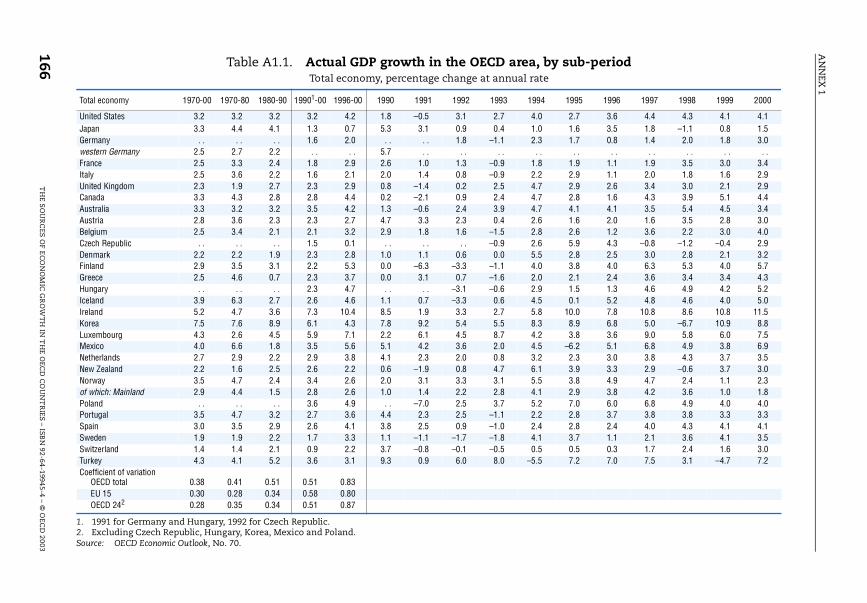
AN
NEX
1
166T
HE S
OU
RC
ES O
F EC
ON
OM
IC G
RO
WT
H IN
TH
E OEC
D C
OU
NT
RIES – ISB
N 92-64-19945-4 – ©
OEC
D 2003
Table A1.1. Actual GDP growth in the OECD area, by sub-periodrate
994 1995 1996 1997 1998 1999 2000
4.0 2.7 3.6 4.4 4.3 4.1 4.11.0 1.6 3.5 1.8 –1.1 0.8 1.52.3 1.7 0.8 1.4 2.0 1.8 3.0
. . . . . . . . . . . . . .1.8 1.9 1.1 1.9 3.5 3.0 3.42.2 2.9 1.1 2.0 1.8 1.6 2.94.7 2.9 2.6 3.4 3.0 2.1 2.94.7 2.8 1.6 4.3 3.9 5.1 4.44.7 4.1 4.1 3.5 5.4 4.5 3.42.6 1.6 2.0 1.6 3.5 2.8 3.02.8 2.6 1.2 3.6 2.2 3.0 4.02.6 5.9 4.3 –0.8 –1.2 –0.4 2.95.5 2.8 2.5 3.0 2.8 2.1 3.24.0 3.8 4.0 6.3 5.3 4.0 5.72.0 2.1 2.4 3.6 3.4 3.4 4.32.9 1.5 1.3 4.6 4.9 4.2 5.24.5 0.1 5.2 4.8 4.6 4.0 5.05.8 10.0 7.8 10.8 8.6 10.8 11.58.3 8.9 6.8 5.0 –6.7 10.9 8.84.2 3.8 3.6 9.0 5.8 6.0 7.54.5 –6.2 5.1 6.8 4.9 3.8 6.93.2 2.3 3.0 3.8 4.3 3.7 3.56.1 3.9 3.3 2.9 –0.6 3.7 3.05.5 3.8 4.9 4.7 2.4 1.1 2.34.1 2.9 3.8 4.2 3.6 1.0 1.85.2 7.0 6.0 6.8 4.9 4.0 4.02.2 2.8 3.7 3.8 3.8 3.3 3.32.4 2.8 2.4 4.0 4.3 4.1 4.14.1 3.7 1.1 2.1 3.6 4.1 3.50.5 0.5 0.3 1.7 2.4 1.6 3.05.5 7.2 7.0 7.5 3.1 –4.7 7.2
Total economy, percentage change at annual
1. 1991 for Germany and Hungary, 1992 for Czech Republic.2. Excluding Czech Republic, Hungary, Korea, Mexico and Poland.Source: OECD Economic Outlook, No. 70.
Total economy 1970-00 1970-80 1980-90 19901-00 1996-00 1990 1991 1992 1993 1
United States 3.2 3.2 3.2 3.2 4.2 1.8 –0.5 3.1 2.7Japan 3.3 4.4 4.1 1.3 0.7 5.3 3.1 0.9 0.4Germany . . . . . . 1.6 2.0 . . . . 1.8 –1.1western Germany 2.5 2.7 2.2 . . . . 5.7 . . . . . .France 2.5 3.3 2.4 1.8 2.9 2.6 1.0 1.3 –0.9Italy 2.5 3.6 2.2 1.6 2.1 2.0 1.4 0.8 –0.9United Kingdom 2.3 1.9 2.7 2.3 2.9 0.8 –1.4 0.2 2.5Canada 3.3 4.3 2.8 2.8 4.4 0.2 –2.1 0.9 2.4Australia 3.3 3.2 3.2 3.5 4.2 1.3 –0.6 2.4 3.9Austria 2.8 3.6 2.3 2.3 2.7 4.7 3.3 2.3 0.4Belgium 2.5 3.4 2.1 2.1 3.2 2.9 1.8 1.6 –1.5Czech Republic . . . . . . 1.5 0.1 . . . . . . –0.9Denmark 2.2 2.2 1.9 2.3 2.8 1.0 1.1 0.6 0.0Finland 2.9 3.5 3.1 2.2 5.3 0.0 –6.3 –3.3 –1.1Greece 2.5 4.6 0.7 2.3 3.7 0.0 3.1 0.7 –1.6Hungary . . . . . . 2.3 4.7 . . . . –3.1 –0.6Iceland 3.9 6.3 2.7 2.6 4.6 1.1 0.7 –3.3 0.6Ireland 5.2 4.7 3.6 7.3 10.4 8.5 1.9 3.3 2.7Korea 7.5 7.6 8.9 6.1 4.3 7.8 9.2 5.4 5.5Luxembourg 4.3 2.6 4.5 5.9 7.1 2.2 6.1 4.5 8.7Mexico 4.0 6.6 1.8 3.5 5.6 5.1 4.2 3.6 2.0Netherlands 2.7 2.9 2.2 2.9 3.8 4.1 2.3 2.0 0.8New Zealand 2.2 1.6 2.5 2.6 2.2 0.6 –1.9 0.8 4.7Norway 3.5 4.7 2.4 3.4 2.6 2.0 3.1 3.3 3.1of which: Mainland 2.9 4.4 1.5 2.8 2.6 1.0 1.4 2.2 2.8Poland . . . . . . 3.6 4.9 . . –7.0 2.5 3.7Portugal 3.5 4.7 3.2 2.7 3.6 4.4 2.3 2.5 –1.1Spain 3.0 3.5 2.9 2.6 4.1 3.8 2.5 0.9 –1.0Sweden 1.9 1.9 2.2 1.7 3.3 1.1 –1.1 –1.7 –1.8Switzerland 1.4 1.4 2.1 0.9 2.2 3.7 –0.8 –0.1 –0.5Turkey 4.3 4.1 5.2 3.6 3.1 9.3 0.9 6.0 8.0 –Coefficient of variation
OECD total 0.38 0.41 0.51 0.51 0.83EU 15 0.30 0.28 0.34 0.58 0.80OECD 242 0.28 0.35 0.34 0.51 0.87
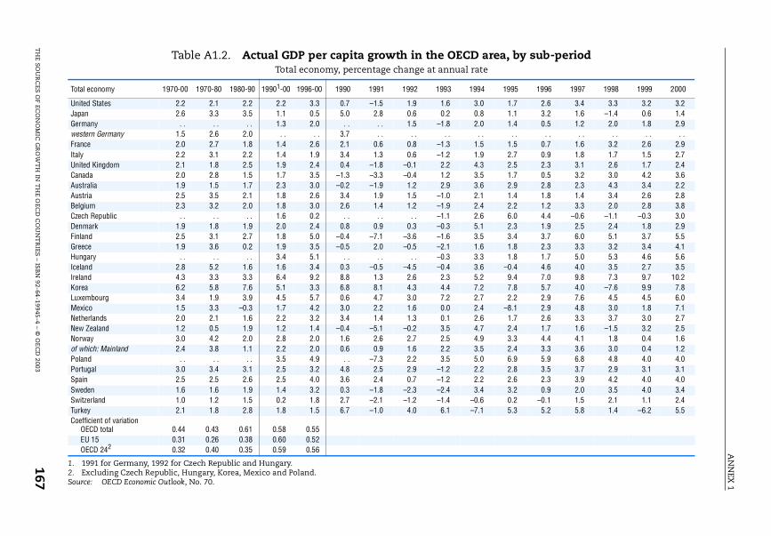
AN
NEX
1
TH
E SOU
RC
ES OF EC
ON
OM
IC G
RO
WT
H IN
TH
E OEC
D C
OU
NT
RIES
– ISB
N 92-64-19945-4 – ©
OE
CD
2003167
Table A1.2. Actual GDP per capita growth in the OECD area, by sub-periodrate
994 1995 1996 1997 1998 1999 2000
3.0 1.7 2.6 3.4 3.3 3.2 3.20.8 1.1 3.2 1.6 –1.4 0.6 1.42.0 1.4 0.5 1.2 2.0 1.8 2.9
. . . . . . . . . . . . . .1.5 1.5 0.7 1.6 3.2 2.6 2.91.9 2.7 0.9 1.8 1.7 1.5 2.74.3 2.5 2.3 3.1 2.6 1.7 2.43.5 1.7 0.5 3.2 3.0 4.2 3.63.6 2.9 2.8 2.3 4.3 3.4 2.22.1 1.4 1.8 1.4 3.4 2.6 2.82.4 2.2 1.2 3.3 2.0 2.8 3.82.6 6.0 4.4 –0.6 –1.1 –0.3 3.05.1 2.3 1.9 2.5 2.4 1.8 2.93.5 3.4 3.7 6.0 5.1 3.7 5.51.6 1.8 2.3 3.3 3.2 3.4 4.13.3 1.8 1.7 5.0 5.3 4.6 5.63.6 –0.4 4.6 4.0 3.5 2.7 3.55.2 9.4 7.0 9.8 7.3 9.7 10.27.2 7.8 5.7 4.0 –7.6 9.9 7.82.7 2.2 2.9 7.6 4.5 4.5 6.02.4 –8.1 2.9 4.8 3.0 1.8 7.12.6 1.7 2.6 3.3 3.7 3.0 2.74.7 2.4 1.7 1.6 –1.5 3.2 2.54.9 3.3 4.4 4.1 1.8 0.4 1.63.5 2.4 3.3 3.6 3.0 0.4 1.25.0 6.9 5.9 6.8 4.8 4.0 4.02.2 2.8 3.5 3.7 2.9 3.1 3.12.2 2.6 2.3 3.9 4.2 4.0 4.03.4 3.2 0.9 2.0 3.5 4.0 3.40.6 0.2 –0.1 1.5 2.1 1.1 2.47.1 5.3 5.2 5.8 1.4 –6.2 5.5
Total economy, percentage change at annual
1. 1991 for Germany, 1992 for Czech Republic and Hungary.2. Excluding Czech Republic, Hungary, Korea, Mexico and Poland.Source: OECD Economic Outlook, No. 70.
Total economy 1970-00 1970-80 1980-90 19901-00 1996-00 1990 1991 1992 1993 1
United States 2.2 2.1 2.2 2.2 3.3 0.7 –1.5 1.9 1.6Japan 2.6 3.3 3.5 1.1 0.5 5.0 2.8 0.6 0.2Germany . . . . . . 1.3 2.0 . . . . 1.5 –1.8western Germany 1.5 2.6 2.0 . . . . 3.7 . . . . . .France 2.0 2.7 1.8 1.4 2.6 2.1 0.6 0.8 –1.3Italy 2.2 3.1 2.2 1.4 1.9 3.4 1.3 0.6 –1.2United Kingdom 2.1 1.8 2.5 1.9 2.4 0.4 –1.8 –0.1 2.2Canada 2.0 2.8 1.5 1.7 3.5 –1.3 –3.3 –0.4 1.2Australia 1.9 1.5 1.7 2.3 3.0 –0.2 –1.9 1.2 2.9Austria 2.5 3.5 2.1 1.8 2.6 3.4 1.9 1.5 –1.0Belgium 2.3 3.2 2.0 1.8 3.0 2.6 1.4 1.2 –1.9Czech Republic . . . . . . 1.6 0.2 . . . . . . –1.1Denmark 1.9 1.8 1.9 2.0 2.4 0.8 0.9 0.3 –0.3Finland 2.5 3.1 2.7 1.8 5.0 –0.4 –7.1 –3.6 –1.6Greece 1.9 3.6 0.2 1.9 3.5 –0.5 2.0 –0.5 –2.1Hungary . . . . . . 3.4 5.1 . . . . . . –0.3Iceland 2.8 5.2 1.6 1.6 3.4 0.3 –0.5 –4.5 –0.4Ireland 4.3 3.3 3.3 6.4 9.2 8.8 1.3 2.6 2.3Korea 6.2 5.8 7.6 5.1 3.3 6.8 8.1 4.3 4.4Luxembourg 3.4 1.9 3.9 4.5 5.7 0.6 4.7 3.0 7.2Mexico 1.5 3.3 –0.3 1.7 4.2 3.0 2.2 1.6 0.0Netherlands 2.0 2.1 1.6 2.2 3.2 3.4 1.4 1.3 0.1New Zealand 1.2 0.5 1.9 1.2 1.4 –0.4 –5.1 –0.2 3.5Norway 3.0 4.2 2.0 2.8 2.0 1.6 2.6 2.7 2.5of which: Mainland 2.4 3.8 1.1 2.2 2.0 0.6 0.9 1.6 2.2Poland . . . . . . 3.5 4.9 . . –7.3 2.2 3.5Portugal 3.0 3.4 3.1 2.5 3.2 4.8 2.5 2.9 –1.2Spain 2.5 2.5 2.6 2.5 4.0 3.6 2.4 0.7 –1.2Sweden 1.6 1.6 1.9 1.4 3.2 0.3 –1.8 –2.3 –2.4Switzerland 1.0 1.2 1.5 0.2 1.8 2.7 –2.1 –1.2 –1.4 –Turkey 2.1 1.8 2.8 1.8 1.5 6.7 –1.0 4.0 6.1 –Coefficient of variation
OECD total 0.44 0.43 0.61 0.58 0.55EU 15 0.31 0.26 0.38 0.60 0.52OECD 242 0.32 0.40 0.35 0.59 0.56
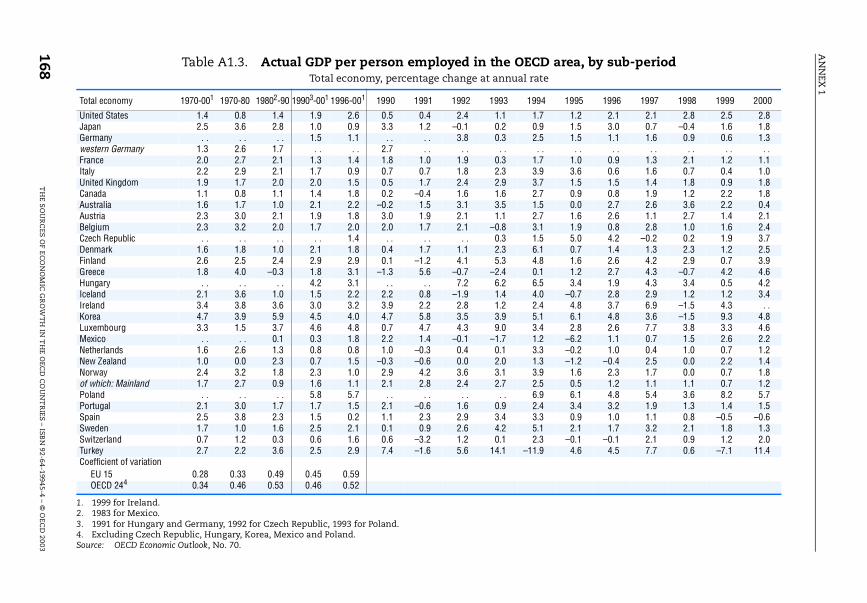
AN
NEX
1
168T
HE S
OU
RC
ES O
F EC
ON
OM
IC G
RO
WT
H IN
TH
E OEC
D C
OU
NT
RIES – ISB
N 92-64-19945-4 – ©
OEC
D 2003
Table A1.3. Actual GDP per person employed in the OECD area, by sub-periodrate
994 1995 1996 1997 1998 1999 2000
1.7 1.2 2.1 2.1 2.8 2.5 2.80.9 1.5 3.0 0.7 –0.4 1.6 1.82.5 1.5 1.1 1.6 0.9 0.6 1.3. . . . . . . . . . . . . .
1.7 1.0 0.9 1.3 2.1 1.2 1.13.9 3.6 0.6 1.6 0.7 0.4 1.03.7 1.5 1.5 1.4 1.8 0.9 1.82.7 0.9 0.8 1.9 1.2 2.2 1.81.5 0.0 2.7 2.6 3.6 2.2 0.42.7 1.6 2.6 1.1 2.7 1.4 2.13.1 1.9 0.8 2.8 1.0 1.6 2.41.5 5.0 4.2 –0.2 0.2 1.9 3.76.1 0.7 1.4 1.3 2.3 1.2 2.54.8 1.6 2.6 4.2 2.9 0.7 3.90.1 1.2 2.7 4.3 –0.7 4.2 4.66.5 3.4 1.9 4.3 3.4 0.5 4.24.0 –0.7 2.8 2.9 1.2 1.2 3.42.4 4.8 3.7 6.9 –1.5 4.3 . .5.1 6.1 4.8 3.6 –1.5 9.3 4.83.4 2.8 2.6 7.7 3.8 3.3 4.61.2 –6.2 1.1 0.7 1.5 2.6 2.23.3 –0.2 1.0 0.4 1.0 0.7 1.21.3 –1.2 –0.4 2.5 0.0 2.2 1.43.9 1.6 2.3 1.7 0.0 0.7 1.82.5 0.5 1.2 1.1 1.1 0.7 1.26.9 6.1 4.8 5.4 3.6 8.2 5.72.4 3.4 3.2 1.9 1.3 1.4 1.53.3 0.9 1.0 1.1 0.8 –0.5 –0.65.1 2.1 1.7 3.2 2.1 1.8 1.32.3 –0.1 –0.1 2.1 0.9 1.2 2.01.9 4.6 4.5 7.7 0.6 –7.1 11.4
Total economy, percentage change at annual
1. 1999 for Ireland.2. 1983 for Mexico.3. 1991 for Hungary and Germany, 1992 for Czech Republic, 1993 for Poland.4. Excluding Czech Republic, Hungary, Korea, Mexico and Poland.Source: OECD Economic Outlook, No. 70.
Total economy 1970-001 1970-80 19802-90 19903-001 1996-001 1990 1991 1992 1993 1
United States 1.4 0.8 1.4 1.9 2.6 0.5 0.4 2.4 1.1Japan 2.5 3.6 2.8 1.0 0.9 3.3 1.2 –0.1 0.2Germany . . . . . . 1.5 1.1 . . . . 3.8 0.3western Germany 1.3 2.6 1.7 . . . . 2.7 . . . . . .France 2.0 2.7 2.1 1.3 1.4 1.8 1.0 1.9 0.3Italy 2.2 2.9 2.1 1.7 0.9 0.7 0.7 1.8 2.3United Kingdom 1.9 1.7 2.0 2.0 1.5 0.5 1.7 2.4 2.9Canada 1.1 0.8 1.1 1.4 1.8 0.2 –0.4 1.6 1.6Australia 1.6 1.7 1.0 2.1 2.2 –0.2 1.5 3.1 3.5Austria 2.3 3.0 2.1 1.9 1.8 3.0 1.9 2.1 1.1Belgium 2.3 3.2 2.0 1.7 2.0 2.0 1.7 2.1 –0.8Czech Republic . . . . . . . . 1.4 . . . . . . 0.3Denmark 1.6 1.8 1.0 2.1 1.8 0.4 1.7 1.1 2.3Finland 2.6 2.5 2.4 2.9 2.9 0.1 –1.2 4.1 5.3Greece 1.8 4.0 –0.3 1.8 3.1 –1.3 5.6 –0.7 –2.4Hungary . . . . . . 4.2 3.1 . . . . 7.2 6.2Iceland 2.1 3.6 1.0 1.5 2.2 2.2 0.8 –1.9 1.4Ireland 3.4 3.8 3.6 3.0 3.2 3.9 2.2 2.8 1.2Korea 4.7 3.9 5.9 4.5 4.0 4.7 5.8 3.5 3.9Luxembourg 3.3 1.5 3.7 4.6 4.8 0.7 4.7 4.3 9.0Mexico . . . . 0.1 0.3 1.8 2.2 1.4 –0.1 –1.7Netherlands 1.6 2.6 1.3 0.8 0.8 1.0 –0.3 0.4 0.1New Zealand 1.0 0.0 2.3 0.7 1.5 –0.3 –0.6 0.0 2.0Norway 2.4 3.2 1.8 2.3 1.0 2.9 4.2 3.6 3.1of which: Mainland 1.7 2.7 0.9 1.6 1.1 2.1 2.8 2.4 2.7Poland . . . . . . 5.8 5.7 . . . . . . . .Portugal 2.1 3.0 1.7 1.7 1.5 2.1 –0.6 1.6 0.9Spain 2.5 3.8 2.3 1.5 0.2 1.1 2.3 2.9 3.4Sweden 1.7 1.0 1.6 2.5 2.1 0.1 0.9 2.6 4.2Switzerland 0.7 1.2 0.3 0.6 1.6 0.6 –3.2 1.2 0.1Turkey 2.7 2.2 3.6 2.5 2.9 7.4 –1.6 5.6 14.1 –1Coefficient of variation
EU 15 0.28 0.33 0.49 0.45 0.59OECD 244 0.34 0.46 0.53 0.46 0.52
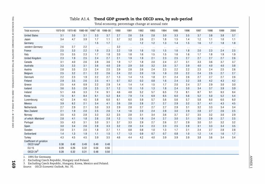
AN
NEX
1
TH
E SOU
RC
ES OF EC
ON
OM
IC G
RO
WT
H IN
TH
E OEC
D C
OU
NT
RIES
– ISB
N 92-64-19945-4 – ©
OE
CD
2003169
Table A1.4. Trend GDP growth in the OECD area, by sub-periodrate
994 1995 1996 1997 1998 1999 2000
3.0 3.3 3.5 3.7 3.8 3.8 3.71.8 1.5 1.4 1.2 1.1 1.0 1.11.3 1.4 1.5 1.6 1.7 1.8 1.8
. . . . . . . . . . . . . .1.5 1.6 1.8 2.0 2.3 2.4 2.51.5 1.6 1.6 1.7 1.8 1.9 1.92.3 2.5 2.7 2.7 2.7 2.7 2.62.4 2.7 3.1 3.3 3.6 3.7 3.73.5 3.7 3.9 4.0 4.0 4.0 3.82.3 2.2 2.2 2.3 2.4 2.5 2.61.9 2.0 2.2 2.4 2.5 2.7 2.72.1 2.4 2.6 2.7 2.7 2.7 2.61.6 2.4 3.2 3.8 4.2 4.3 4.21.7 2.0 2.4 2.7 2.9 3.0 3.01.8 2.4 3.0 3.4 3.7 3.9 3.96.5 7.3 8.1 8.7 9.1 9.3 9.46.5 6.0 5.6 5.2 5.0 5.2 5.45.6 5.6 5.7 5.8 6.0 6.0 6.02.7 2.9 3.2 3.7 4.1 4.3 4.52.7 2.9 3.1 3.2 3.3 3.4 3.42.8 3.0 2.9 2.8 2.7 2.6 2.53.6 3.7 3.7 3.5 3.2 3.0 2.92.7 3.0 3.1 3.0 2.9 2.7 2.52.6 2.7 2.9 3.0 3.1 3.2 3.22.3 2.5 2.8 3.1 3.3 3.4 3.51.3 1.7 2.1 2.4 2.7 2.8 2.80.7 0.8 1.0 1.2 1.4 1.6 1.73.9 3.9 3.9 3.8 3.6 3.4 3.4
Total economy, percentage change at annual
1. 1991 for Germany.2. Excluding Czech Republic, Hungary and Poland.3. Excluding Czech Republic, Hungary, Korea, Mexico and Poland.Source: OECD Economic Outlook, No. 70.
Total economy 1970-00 1970-80 1980-90 19901-00 1996-00 1990 1991 1992 1993 1
United States 3.1 3.0 3.1 3.3 3.7 2.7 2.6 2.6 2.8Japan 3.4 4.7 3.9 1.7 1.1 3.7 3.2 2.6 2.1Germany . . . . . . 1.5 1.7 . . . . 1.2 1.2western Germany 2.6 2.7 2.2 . . . . 3.2 . . . . . .France 2.5 3.3 2.2 1.9 2.3 2.2 1.9 1.6 1.5Italy 2.5 3.5 2.3 1.7 1.8 2.0 1.8 1.6 1.5United Kingdom 2.3 1.9 2.5 2.4 2.7 2.1 1.9 1.9 2.1Canada 3.1 4.0 2.6 2.8 3.6 1.9 1.7 1.8 2.0Australia 3.3 3.3 3.1 3.6 4.0 2.9 2.9 3.0 3.2Austria 2.8 3.5 2.3 2.4 2.5 2.9 2.8 2.6 2.4Belgium 2.5 3.2 2.1 2.2 2.6 2.4 2.2 2.0 1.9Denmark 2.2 2.3 1.9 2.2 2.7 1.3 1.4 1.5 1.8Finland 2.9 3.5 2.6 2.5 4.1 0.7 0.2 0.3 0.8Greece 2.5 4.4 0.9 2.2 2.9 1.4 1.4 1.4 1.5Iceland 3.6 5.5 2.8 2.5 3.7 1.2 1.0 1.0 1.3Ireland 5.1 4.6 3.3 7.4 9.1 4.6 4.8 5.2 5.7Korea 7.5 8.1 8.4 6.1 5.2 8.4 7.9 7.4 6.9Luxembourg 4.2 2.4 4.5 5.8 6.0 6.1 6.0 5.9 5.7Mexico 3.9 6.2 2.1 3.4 4.1 2.6 2.8 2.8 2.7Netherlands 2.7 2.9 2.1 3.0 3.3 2.9 2.8 2.7 2.7New Zealand 2.1 1.9 2.0 2.5 2.6 1.4 1.6 2.0 2.4Norway 3.5 4.3 2.8 3.3 3.2 2.5 2.8 3.1 3.4of which: Mainland 2.8 4.1 1.8 2.6 2.8 1.2 1.5 1.9 2.4Portugal 3.5 4.3 3.1 3.0 3.1 3.7 3.3 2.9 2.7Spain 3.0 3.4 2.6 2.8 3.3 3.2 2.8 2.4 2.3Sweden 2.0 2.1 2.0 1.8 2.7 1.1 0.8 0.8 1.0Switzerland 1.4 1.3 1.9 1.1 1.5 1.7 1.3 0.9 0.7Turkey 4.3 4.5 4.5 3.9 3.5 4.6 4.4 4.2 4.0Coefficient of variation
OECD total2 0.38 0.40 0.49 0.49 0.48EU 15 0.29 0.26 0.32 0.56 0.56OECD 243 0.28 0.32 0.31 0.48 0.50
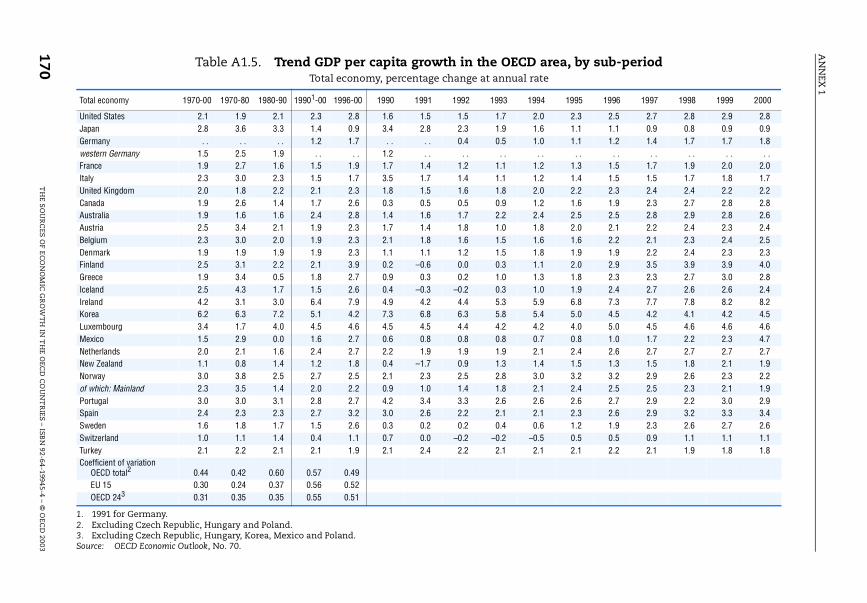
AN
NEX
1
170T
HE S
OU
RC
ES O
F EC
ON
OM
IC G
RO
WT
H IN
TH
E OEC
D C
OU
NT
RIES – ISB
N 92-64-19945-4 – ©
OEC
D 2003
Table A1.5. Trend GDP per capita growth in the OECD area, by sub-periodrate
994 1995 1996 1997 1998 1999 2000
2.0 2.3 2.5 2.7 2.8 2.9 2.81.6 1.1 1.1 0.9 0.8 0.9 0.91.0 1.1 1.2 1.4 1.7 1.7 1.8
. . . . . . . . . . . . . .1.2 1.3 1.5 1.7 1.9 2.0 2.01.2 1.4 1.5 1.5 1.7 1.8 1.72.0 2.2 2.3 2.4 2.4 2.2 2.21.2 1.6 1.9 2.3 2.7 2.8 2.82.4 2.5 2.5 2.8 2.9 2.8 2.61.8 2.0 2.1 2.2 2.4 2.3 2.41.6 1.6 2.2 2.1 2.3 2.4 2.51.8 1.9 1.9 2.2 2.4 2.3 2.31.1 2.0 2.9 3.5 3.9 3.9 4.01.3 1.8 2.3 2.3 2.7 3.0 2.81.0 1.9 2.4 2.7 2.6 2.6 2.45.9 6.8 7.3 7.7 7.8 8.2 8.25.4 5.0 4.5 4.2 4.1 4.2 4.54.2 4.0 5.0 4.5 4.6 4.6 4.60.7 0.8 1.0 1.7 2.2 2.3 4.72.1 2.4 2.6 2.7 2.7 2.7 2.71.4 1.5 1.3 1.5 1.8 2.1 1.93.0 3.2 3.2 2.9 2.6 2.3 2.22.1 2.4 2.5 2.5 2.3 2.1 1.92.6 2.6 2.7 2.9 2.2 3.0 2.92.1 2.3 2.6 2.9 3.2 3.3 3.40.6 1.2 1.9 2.3 2.6 2.7 2.60.5 0.5 0.5 0.9 1.1 1.1 1.12.1 2.1 2.2 2.1 1.9 1.8 1.8
Total economy, percentage change at annual
1. 1991 for Germany.2. Excluding Czech Republic, Hungary and Poland.3. Excluding Czech Republic, Hungary, Korea, Mexico and Poland.Source: OECD Economic Outlook, No. 70.
Total economy 1970-00 1970-80 1980-90 19901-00 1996-00 1990 1991 1992 1993 1
United States 2.1 1.9 2.1 2.3 2.8 1.6 1.5 1.5 1.7Japan 2.8 3.6 3.3 1.4 0.9 3.4 2.8 2.3 1.9Germany . . . . . . 1.2 1.7 . . . . 0.4 0.5western Germany 1.5 2.5 1.9 . . . . 1.2 . . . . . .France 1.9 2.7 1.6 1.5 1.9 1.7 1.4 1.2 1.1Italy 2.3 3.0 2.3 1.5 1.7 3.5 1.7 1.4 1.1United Kingdom 2.0 1.8 2.2 2.1 2.3 1.8 1.5 1.6 1.8Canada 1.9 2.6 1.4 1.7 2.6 0.3 0.5 0.5 0.9Australia 1.9 1.6 1.6 2.4 2.8 1.4 1.6 1.7 2.2Austria 2.5 3.4 2.1 1.9 2.3 1.7 1.4 1.8 1.0Belgium 2.3 3.0 2.0 1.9 2.3 2.1 1.8 1.6 1.5Denmark 1.9 1.9 1.9 1.9 2.3 1.1 1.1 1.2 1.5Finland 2.5 3.1 2.2 2.1 3.9 0.2 –0.6 0.0 0.3Greece 1.9 3.4 0.5 1.8 2.7 0.9 0.3 0.2 1.0Iceland 2.5 4.3 1.7 1.5 2.6 0.4 –0.3 –0.2 0.3Ireland 4.2 3.1 3.0 6.4 7.9 4.9 4.2 4.4 5.3Korea 6.2 6.3 7.2 5.1 4.2 7.3 6.8 6.3 5.8Luxembourg 3.4 1.7 4.0 4.5 4.6 4.5 4.5 4.4 4.2Mexico 1.5 2.9 0.0 1.6 2.7 0.6 0.8 0.8 0.8Netherlands 2.0 2.1 1.6 2.4 2.7 2.2 1.9 1.9 1.9New Zealand 1.1 0.8 1.4 1.2 1.8 0.4 –1.7 0.9 1.3Norway 3.0 3.8 2.5 2.7 2.5 2.1 2.3 2.5 2.8of which: Mainland 2.3 3.5 1.4 2.0 2.2 0.9 1.0 1.4 1.8Portugal 3.0 3.0 3.1 2.8 2.7 4.2 3.4 3.3 2.6Spain 2.4 2.3 2.3 2.7 3.2 3.0 2.6 2.2 2.1Sweden 1.6 1.8 1.7 1.5 2.6 0.3 0.2 0.2 0.4Switzerland 1.0 1.1 1.4 0.4 1.1 0.7 0.0 –0.2 –0.2 –Turkey 2.1 2.2 2.1 2.1 1.9 2.1 2.4 2.2 2.1Coefficient of variation
OECD total2 0.44 0.42 0.60 0.57 0.49EU 15 0.30 0.24 0.37 0.56 0.52OECD 243 0.31 0.35 0.35 0.55 0.51
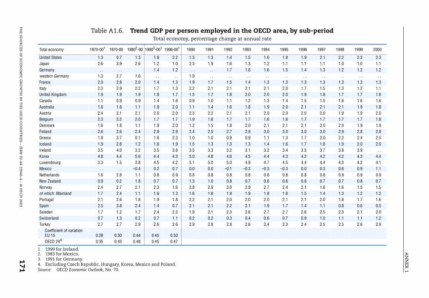
AN
NEX
1
TH
E SOU
RC
ES OF EC
ON
OM
IC G
RO
WT
H IN
TH
E OEC
D C
OU
NT
RIES
– ISB
N 92-64-19945-4 – ©
OE
CD
2003171
Table A1.6. Trend GDP per person employed in the OECD area, by sub-periodrate
994 1995 1996 1997 1998 1999 2000
1.6 1.8 1.9 2.1 2.2 2.3 2.31.2 1.1 1.1 1.1 1.0 1.0 1.11.6 1.5 1.4 1.3 1.2 1.2 1.2
. . . . . . . . . . . . . .1.3 1.3 1.3 1.3 1.3 1.3 1.32.1 2.0 1.7 1.5 1.3 1.2 1.12.0 2.0 1.9 1.8 1.7 1.7 1.61.3 1.4 1.5 1.5 1.6 1.6 1.61.9 2.0 2.1 2.1 2.1 1.9 1.82.0 2.0 2.0 2.0 1.9 1.9 2.01.6 1.6 1.7 1.7 1.7 1.7 1.82.1 2.1 2.1 2.0 2.0 1.9 1.93.0 3.0 3.0 3.0 2.9 2.8 2.81.1 1.3 1.7 2.0 2.2 2.4 2.51.4 1.6 1.7 1.8 1.9 2.0 2.03.2 3.4 3.5 3.7 3.8 3.9 . .4.4 4.3 4.2 4.2 4.2 4.3 4.44.7 4.5 4.4 4.4 4.3 4.2 4.10.3 –0.3 0.0 0.3 0.6 0.9 1.10.8 0.8 0.8 0.8 0.9 0.9 0.90.6 0.6 0.6 0.7 0.7 0.8 0.72.7 2.4 2.1 1.8 1.6 1.5 1.51.8 1.6 1.5 1.4 1.3 1.2 1.22.0 2.1 2.1 2.0 1.8 1.7 1.61.9 1.7 1.4 1.1 0.8 0.6 0.52.7 2.7 2.6 2.5 2.3 2.1 2.00.6 0.7 0.9 1.0 1.1 1.1 1.22.4 2.3 2.4 2.5 2.5 2.6 2.9
Total economy, percentage change at annual
1. 1999 for Ireland.2. 1983 for Mexico.3. 1991 for Germany.4. Excluding Czech Republic, Hungary, Korea, Mexico and Poland.Source: OECD Economic Outlook, No. 70.
Total economy 1970-001 1970-80 19802-90 19903-001 1996-001 1990 1991 1992 1993 1
United States 1.3 0.7 1.3 1.8 2.2 1.3 1.3 1.4 1.5Japan 2.6 3.9 2.6 1.2 1.0 2.3 1.9 1.6 1.3Germany . . . . 1.4 1.2 . . . . 1.7 1.6western Germany 1.3 2.7 1.6 . . . . 1.9 . . . . . .France 2.0 2.8 2.0 1.4 1.3 1.9 1.7 1.5 1.4Italy 2.3 2.9 2.2 1.7 1.3 2.2 2.1 2.1 2.1United Kingdom 1.9 1.9 1.9 1.8 1.7 1.5 1.7 1.8 2.0Canada 1.1 0.9 0.9 1.4 1.6 0.9 1.0 1.1 1.2Australia 1.6 1.8 1.1 1.9 2.0 1.1 1.4 1.6 1.8Austria 2.4 3.1 2.1 2.0 2.0 2.3 2.2 2.1 2.1Belgium 2.3 3.2 2.0 1.7 1.7 1.9 1.8 1.7 1.7Denmark 1.6 1.8 1.1 1.9 2.0 1.2 1.5 1.8 2.0Finland 2.6 2.6 2.4 2.9 2.9 2.4 2.5 2.7 2.9Greece 1.8 3.7 0.1 1.6 2.3 1.0 1.0 0.9 0.9Iceland 1.9 2.8 1.2 1.6 1.9 1.5 1.3 1.3 1.3Ireland 3.5 4.0 3.2 3.5 3.8 3.5 3.3 3.2 3.1Korea 4.8 4.4 5.6 4.4 4.3 5.0 4.8 4.6 4.5Luxembourg 3.3 1.5 3.8 4.5 4.2 5.1 5.0 5.0 4.9Mexico . . . . –0.4 0.2 0.7 0.0 0.0 –0.1 –0.3 –Netherlands 1.6 2.8 1.1 0.8 0.9 0.8 0.8 0.8 0.8New Zealand 0.9 0.2 1.8 0.7 0.7 1.3 1.0 0.8 0.7Norway 2.4 2.7 2.1 2.3 1.6 2.8 2.9 3.0 2.9of which: Mainland 1.7 2.4 1.1 1.6 1.3 1.6 1.8 1.9 1.9Portugal 2.1 2.6 1.8 1.9 1.8 2.2 2.1 2.0 2.0Spain 2.5 3.8 2.4 1.4 0.7 2.1 2.1 2.2 2.1Sweden 1.7 1.2 1.7 2.4 2.2 1.9 2.1 2.3 2.6Switzerland 0.7 1.3 0.2 0.7 1.1 0.2 0.2 0.3 0.4Turkey 2.7 2.7 2.9 2.6 2.6 2.9 2.8 2.8 2.6
Coefficient of variation EU 15 0.28 0.30 0.44 0.45 0.50OECD 244 0.35 0.43 0.48 0.45 0.47
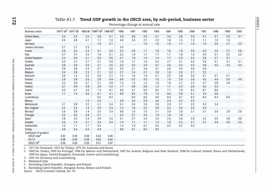
AN
NEX
1
172T
HE S
OU
RC
ES O
F EC
ON
OM
IC G
RO
WT
H IN
TH
E OEC
D C
OU
NT
RIES – ISB
N 92-64-19945-4 – ©
OEC
D 2003
Table A1.7. Trend GDP growth in the OECD area, by sub-period, business sector
Zealand, 1998 for Iceland, Ireland, Korea and Netherlands,
994 1995 1996 1997 1998 1999 2000
3.4 3.6 3.9 4.1 4.1 4.2 4.11.8 1.5 1.3 1.1 1.0 1.0 . .1.6 1.7 1.8 1.9 2.0 2.1 2.2
. . . . . . . . . . . . . .1.6 1.8 2.0 2.3 2.5 2.7 2.81.7 1.8 1.9 2.0 2.1 2.2 2.21.7 2.0 2.3 2.6 2.7 2.7 . .2.7 3.1 3.5 3.8 4.1 4.1 4.14.0 4.3 4.5 4.6 4.5 4.4 4.32.6 2.5 2.6 2.6 . . . . . .1.9 2.0 2.1 2.2 . . . . . .2.5 2.8 3.0 3.1 3.1 3.1 . .1.9 2.9 3.8 4.5 4.9 5.0 4.91.8 2.1 2.4 2.7 2.9 2.9 . .1.7 2.3 2.8 3.2 3.3 . . . .7.1 7.8 8.4 8.7 8.8 . . . .6.6 5.9 5.1 4.4 3.9 . . . .6.0 6.1 6.2 6.3 6.4 6.4 . .2.3 2.2 2.2 . . . . . . . .2.9 3.1 3.2 3.3 3.4 . . . .3.3 3.5 3.5 3.3 . . . . . .2.6 2.9 3.1 3.1 3.0 2.8 2.61.8 1.8 . . . . . . . . . .2.4 2.6 2.9 3.2 3.5 3.6 3.61.8 2.3 2.7 3.1 3.4 3.5 3.50.3 0.3 0.3 . . . . . . . .
. . . . . . . . . . . . . .
Percentage change at annual rate
1. 1971 for Denmark, 1972 for Turkey, 1975 for Australia and Korea.2. 1993 for Turkey, 1995 for Portugal, 1996 for Mexico and Switzerland, 1997 for Austria, Belgium and New
1999 for Japan, United Kingdom, Denmark, Greece and Luxembourg.3. 1991 for Germany and Luxembourg.4. Mainland only.5. Excluding Czech Republic, Hungary and Poland.6. Excluding Czech Republic, Hungary, Korea, Mexico and Poland.Source: OECD Economic Outlook, No. 70.
Business sector 19701-002 19701-80 1980-90 19903-002 1996-002 1990 1991 1992 1993 1
United States 3.4 3.2 3.3 3.6 4.1 2.8 2.8 2.9 3.1Japan 3.6 4.8 4.1 1.7 1.0 4.0 3.4 2.7 2.2Germany . . . . . . 1.8 2.1 . . . . 1.5 1.5western Germany 2.7 2.7 2.3 . . . . 3.4 . . . . . .France 2.6 3.5 2.3 2.1 2.6 2.3 2.0 1.7 1.6Italy 2.7 3.7 2.5 1.9 2.1 2.2 1.9 1.7 1.7United Kingdom 2.4 2.0 3.1 2.0 2.6 2.1 1.6 1.4 1.4Canada 3.3 4.1 2.7 3.1 4.0 1.8 1.7 1.8 2.2Australia 3.6 2.9 3.5 4.1 4.5 3.3 3.3 3.4 3.7Austria 2.9 3.6 2.4 2.7 2.6 3.2 3.1 2.9 2.7Belgium 2.4 2.8 2.3 2.1 2.2 2.7 2.4 2.1 2.0Denmark 2.0 1.3 2.2 2.6 3.1 1.5 1.6 1.8 2.1Finland 2.8 2.8 2.6 2.9 4.9 0.6 0.2 0.3 1.0Greece 2.2 3.9 0.7 2.1 2.8 1.3 1.4 1.5 1.6Iceland 3.7 5.9 2.8 2.0 3.3 1.1 0.8 0.8 1.2Ireland 5.2 4.7 4.0 7.4 8.7 5.6 5.7 6.0 6.5Korea 7.7 7.5 9.2 6.1 4.1 8.9 8.3 7.8 7.2Luxembourg . . . . . . 6.2 6.4 . . 6.0 6.0 6.0Mexico . . . . 1.3 2.5 . . 2.9 3.0 2.9 2.6Netherlands 2.7 2.8 2.2 3.1 3.4 3.1 3.0 2.9 2.9New Zealand 2.2 2.2 1.3 2.9 3.3 1.2 1.6 2.2 2.8Norway4 2.6 3.8 1.4 2.5 2.9 0.6 1.0 1.5 2.1Portugal 3.2 4.2 2.8 2.1 . . 3.3 2.7 2.2 1.9Spain 2.8 3.2 2.4 2.9 3.5 3.1 2.7 2.4 2.3Sweden 2.0 1.4 2.1 2.4 3.4 1.4 1.1 1.1 1.3Switzerland 1.2 1.1 1.7 0.5 . . 1.3 1.0 0.7 0.4Turkey 4.6 3.4 5.5 5.0 . . 9.8 0.7 6.2 8.3Coefficient of variation
OECD total5 0.42 0.42 0.59 0.52 0.46EU 15 0.28 0.33 0.29 0.55 0.52OECD 246 0.30 0.36 0.39 0.51 0.47
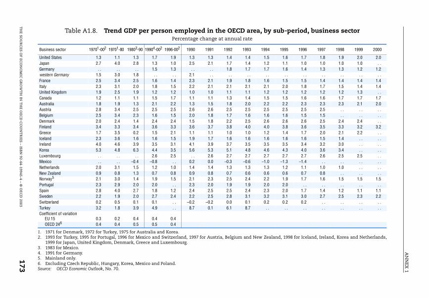
AN
NEX
1
TH
E SOU
RC
ES OF EC
ON
OM
IC G
RO
WT
H IN
TH
E OEC
D C
OU
NT
RIES
– ISB
N 92-64-19945-4 – ©
OE
CD
2003173
Table A1.8. Trend GDP per person employed in the OECD area, by sub-period, business sector
Zealand, 1998 for Iceland, Ireland, Korea and Netherlands,
994 1995 1996 1997 1998 1999 2000
1.5 1.6 1.7 1.8 1.9 2.0 2.01.2 1.1 1.0 1.0 1.0 1.0 . .1.7 1.6 1.4 1.3 1.3 1.2 1.2
. . . . . . . . . . . . . .1.6 1.5 1.5 1.4 1.4 1.4 1.42.1 2.0 1.8 1.7 1.5 1.4 1.41.2 1.2 1.2 1.2 1.2 1.3 . .1.5 1.5 1.6 1.6 1.7 1.7 1.72.2 2.2 2.3 2.3 2.3 2.1 2.02.5 2.5 2.5 2.5 . . . . . .1.6 1.6 1.5 1.5 . . . . . .2.6 2.6 2.6 2.5 2.4 2.4 . .4.0 3.8 3.6 3.5 3.3 3.2 3.21.2 1.4 1.7 2.0 2.1 2.2 . .1.6 1.6 1.6 1.5 1.4 . . . .3.5 3.5 3.4 3.2 3.0 . . . .4.6 4.3 4.0 3.6 3.4 . . . .2.7 2.7 2.7 2.6 2.5 2.5 . .1.0 –1.3 –1.4 . . . . . . . .1.3 1.2 1.1 1.0 1.0 . . . .0.6 0.6 0.7 0.8 . . . . . .2.2 1.9 1.7 1.6 1.5 1.5 1.52.0 2.0 . . . . . . . . . .2.3 2.0 1.7 1.4 1.2 1.1 1.13.2 3.1 3.0 2.7 2.5 2.3 2.20.2 0.2 0.2 . . . . . . . .
. . . . . . . . . . . . . .
Percentage change at annual rate
1. 1971 for Denmark, 1972 for Turkey, 1975 for Australia and Korea.2. 1993 for Turkey, 1995 for Portugal, 1996 for Mexico and Switzerland, 1997 for Austria, Belgium and New
1999 for Japan, United Kingdom, Denmark, Greece and Luxembourg.3. 1983 for Mexico.4. 1991 for Germany.5. Mainland only.6. Excluding Czech Republic, Hungary, Korea, Mexico and Poland.Source: OECD Economic Outlook, No. 70.
Business sector 19701-002 19701-80 19803-90 19904-002 1996-002 1990 1991 1992 1993 1
United States 1.3 1.1 1.3 1.7 1.9 1.3 1.3 1.4 1.4Japan 2.7 4.0 2.8 1.3 1.0 2.5 2.1 1.7 1.4Germany . . . . . . 1.5 1.3 . . . . 1.8 1.7western Germany 1.5 3.0 1.8 . . . . 2.1 . . . . . .France 2.5 3.4 2.5 1.6 1.4 2.3 2.1 1.9 1.8Italy 2.3 3.1 2.0 1.8 1.5 2.2 2.1 2.1 2.1United Kingdom 1.9 2.5 1.9 1.2 1.2 1.0 1.0 1.1 1.1Canada 1.2 1.1 1.1 1.5 1.7 1.1 1.1 1.3 1.4Australia 1.8 1.9 1.3 2.1 2.2 1.3 1.5 1.8 2.0Austria 2.8 3.4 2.5 2.5 2.5 2.6 2.6 2.5 2.5Belgium 2.5 3.4 2.3 1.6 1.5 2.0 1.8 1.7 1.6Denmark 2.0 2.4 1.4 2.4 2.4 1.5 1.8 2.2 2.5Finland 3.4 3.3 3.4 3.6 3.3 3.6 3.7 3.8 4.0Greece 1.7 3.5 0.2 1.5 2.1 1.1 1.1 1.0 1.0Iceland 2.3 3.6 1.6 1.6 1.5 1.9 1.7 1.6 1.6Ireland 4.0 4.6 3.9 3.5 3.1 4.1 3.9 3.7 3.5Korea 5.3 4.8 6.3 4.4 3.5 5.6 5.3 5.1 4.8Luxembourg . . . . . . 2.6 2.5 . . 2.6 2.7 2.7Mexico . . . . –0.4 –0.8 . . 0.2 0.0 –0.3 –0.6 –Netherlands 2.0 3.1 1.5 1.2 1.0 1.4 1.4 1.3 1.3New Zealand 0.9 0.8 1.3 0.7 0.8 0.9 0.8 0.7 0.6Norway5 2.1 3.0 1.4 1.9 1.5 2.1 2.3 2.5 2.4Portugal 2.3 2.9 2.0 2.0 . . 2.3 2.0 1.9 1.9Spain 2.8 4.0 2.7 1.8 1.2 2.4 2.5 2.5 2.4Sweden 2.2 1.9 2.0 2.7 2.4 2.2 2.5 2.8 3.1Switzerland 0.2 0.5 0.1 0.1 . . –0.2 –0.2 0.0 0.1Turkey 3.2 1.8 3.9 4.9 . . 8.7 0.1 6.1 8.7Coefficient of variation
EU 15 0.3 0.2 0.4 0.4 0.4OECD 246 0.4 0.4 0.5 0.5 0.4
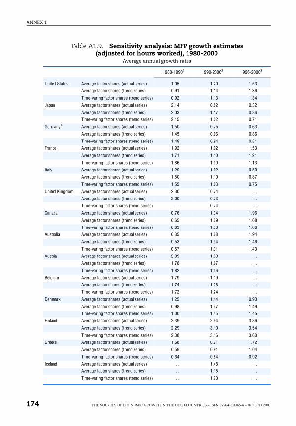
ANNEX 1
3
Table A1.9. Sensitivity analysis: MFP growth estimates (adjusted for hours worked), 1980-2000
Average annual growth rates
1980-19901 1990-20002 1996-2000
United States Average factor shares (actual series) 1.05 1.20 1.53
Average factor shares (trend series) 0.91 1.14 1.36
Time-varing factor shares (trend series) 0.92 1.13 1.34
Japan Average factor shares (actual series) 2.14 0.82 0.32
Average factor shares (trend series) 2.03 1.17 0.86
Time-varing factor shares (trend series) 2.15 1.02 0.71
Germany4 Average factor shares (actual series) 1.50 0.75 0.63
Average factor shares (trend series) 1.45 0.96 0.86
Time-varing factor shares (trend series) 1.49 0.94 0.81
France Average factor shares (actual series) 1.92 1.02 1.53
Average factor shares (trend series) 1.71 1.10 1.21
Time-varing factor shares (trend series) 1.86 1.00 1.13
Italy Average factor shares (actual series) 1.29 1.02 0.50
Average factor shares (trend series) 1.50 1.10 0.87
Time-varing factor shares (trend series) 1.55 1.03 0.75
United Kingdom Average factor shares (actual series) 2.30 0.74 . .
Average factor shares (trend series) 2.00 0.73 . .
Time-varing factor shares (trend series) . . 0.74 . .
Canada Average factor shares (actual series) 0.76 1.34 1.96
Average factor shares (trend series) 0.65 1.29 1.68
Time-varing factor shares (trend series) 0.63 1.30 1.66
Australia Average factor shares (actual series) 0.35 1.68 1.94
Average factor shares (trend series) 0.53 1.34 1.46
Time-varing factor shares (trend series) 0.57 1.31 1.43
Austria Average factor shares (actual series) 2.09 1.39 . .
Average factor shares (trend series) 1.78 1.67 . .
Time-varing factor shares (trend series) 1.82 1.56 . .
Belgium Average factor shares (actual series) 1.79 1.19 . .
Average factor shares (trend series) 1.74 1.28 . .
Time-varing factor shares (trend series) 1.72 1.24 . .
Denmark Average factor shares (actual series) 1.25 1.44 0.93
Average factor shares (trend series) 0.98 1.47 1.49
Time-varing factor shares (trend series) 1.00 1.45 1.45
Finland Average factor shares (actual series) 2.39 2.94 3.86
Average factor shares (trend series) 2.29 3.10 3.54
Time-varing factor shares (trend series) 2.38 3.16 3.60
Greece Average factor shares (actual series) 1.68 0.71 1.72
Average factor shares (trend series) 0.59 0.91 1.04
Time-varing factor shares (trend series) 0.64 0.84 0.92
Iceland Average factor shares (actual series) . . 1.48 . .
Average factor shares (trend series) . . 1.15 . .
Time-varing factor shares (trend series) . . 1.20 . .
174 THE SOURCES OF ECONOMIC GROWTH IN THE OECD COUNTRIES – ISBN 92-64-19945-4 – © OECD 2003
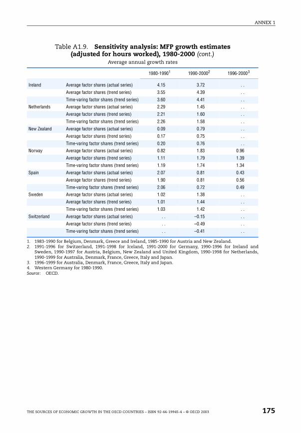
ANNEX 1
Table A1.9. Sensitivity analysis: MFP growth estimates (adjusted for hours worked), 1980-2000 (cont.)
Average annual growth rates
1. 1983-1990 for Belgium, Denmark, Greece and Ireland, 1985-1990 for Austria and New Zealand.2. 1991-1996 for Switzerland, 1991-1998 for Iceland, 1991-2000 for Germany, 1990-1996 for Ireland and
Sweden, 1990-1997 for Austria, Belgium, New Zealand and United Kingdom, 1990-1998 for Netherlands,1990-1999 for Australia, Denmark, France, Greece, Italy and Japan.
3. 1996-1999 for Australia, Denmark, France, Greece, Italy and Japan.4. Western Germany for 1980-1990.Source: OECD.
1980-19901 1990-20002 1996-20003
Ireland Average factor shares (actual series) 4.15 3.72 . .
Average factor shares (trend series) 3.55 4.39 . .
Time-varing factor shares (trend series) 3.60 4.41 . .
Netherlands Average factor shares (actual series) 2.29 1.45 . .
Average factor shares (trend series) 2.21 1.60 . .
Time-varing factor shares (trend series) 2.26 1.58 . .
New Zealand Average factor shares (actual series) 0.09 0.79 . .
Average factor shares (trend series) 0.17 0.75 . .
Time-varing factor shares (trend series) 0.20 0.76 . .
Norway Average factor shares (actual series) 0.82 1.83 0.96
Average factor shares (trend series) 1.11 1.79 1.39
Time-varing factor shares (trend series) 1.19 1.74 1.34
Spain Average factor shares (actual series) 2.07 0.81 0.43
Average factor shares (trend series) 1.90 0.81 0.56
Time-varing factor shares (trend series) 2.06 0.72 0.49
Sweden Average factor shares (actual series) 1.02 1.38 . .
Average factor shares (trend series) 1.01 1.44 . .
Time-varing factor shares (trend series) 1.03 1.42 . .
Switzerland Average factor shares (actual series) . . –0.15 . .
Average factor shares (trend series) . . –0.49 . .
Time-varing factor shares (trend series) . . –0.41 . .
THE SOURCES OF ECONOMIC GROWTH IN THE OECD COUNTRIES – ISBN 92-64-19945-4 – © OECD 2003 175
ANNEX 1
Notes
1. For a fuller description, see Bassanini et al., (2000); Colecchia and Schreyer (2002).
2. It should also be stressed that aggregation through (however defined) user costsassumes that assets are homogeneous. This implies that different vintages of thesame machine should be counted as different assets, while their current prices(expressed in terms of the output deflator) appear in equation [A.1.4]. In practice,however, this would introduce unsolvable problems in the construction of growthrates for new machines. As a solution, Jorgenson and Griliches (1967) suggestextending the foregoing procedure to aggregate different vintages of the sameasset through the use of hedonic price indexes. In this way the aggregate flow ofcapital services of each asset across all vintages can be seen as proportional to theexisting stock of that capital asset expressed in efficiency units.
3. Scarpetta et al. (2000) also compare trend series obtained with this approach withthose obtained extending the time series by means of the OECD Medium TermReference Scenario (MTRS). The results are broadly similar, although in a fewinstances estimated growth rates for the most recent years show somedifferences. Amongst the G-7 countries, trend GDP growth rates for Japan in 2000will be somewhat lower using MTRS, while significant differences for 1999and 2000 are also found for Ireland, Korea, Mexico and Turkey (with lower GDPgrowth rates obtained by using MTRS) as well as Greece (with higher GDP growthrate obtained by using MTRS).
4. The use of both is not frequent in the literature: the Phillips curve has been usedmore widely (e.g. Gordon, 1997, and OECD, 1999a, 1999b), however Okun’s law hasbeen used by Moosa (1997). Laxton and Tetlow (1992), Conway and Hunt (1997) andApel and Jansson (1999) use both.
176 THE SOURCES OF ECONOMIC GROWTH IN THE OECD COUNTRIES – ISBN 92-64-19945-4 – © OECD 2003
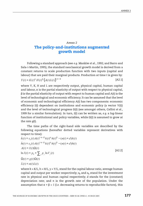
ANNEX 2
Annex 2
The policy-and-institutions augmented growth model
Following a standard approach (see e.g. Mankiw et al., 1992; and Barro andSala-i-Martin, 1995), the standard neoclassical growth model is derived from aconstant returns to scale production function with two inputs (capital andlabour) that are paid their marginal products. Production at time t is given by:
where Y, K, H and L are respectively output, physical capital, human capitaland labour, α is the partial elasticity of output with respect to physical capital,β is the partial elasticity of output with respect to human capital and A(t) is thelevel of technological and economic efficiency. It can be assumed that the levelof economic and technological efficiency A(t) has two components: economicefficiency I(t) dependent on institutions and economic policy (a vector V(t))and the level of technological progress Ω(t) (see amongst others, Cellini et al.,1999 for a similar formulation). In turn, I(t) can be written as, e.g. a log-linearfunction of institutional and policy variables, while Ω(t) is assumed to grow atthe rate g(t).
The time paths of the right-hand side variables are described by thefollowing equations (hereafter dotted variables represent derivatives withrespect to time):
where k = K/L, h = H/L, y = Y/L, stand for the capital labour ratio, average humancapital and output per worker respectively; sk and sh stand for the investmentrate in physical and human capital respectively; d stands for the (constant)
depreciation rate; and n is the growth rate of the population. Under theassumption that α + β < 1 (i.e. decreasing returns to reproducible factors), this
( ) βαβα −−= 1)()()()()( tLtAtHtKtY [A2.1]
)()()(
)()()(
)(ln)(ln
)()()(
)())(()()()()()(
)())(()()()()()(
0
1
1
tLtntL
ttgt
tVpptI
ttItA
thdtnthtktAtsth
tkdtnthtktAtstk
j jj
h
k
=Ω=Ω
+=Ω=
+−=
+−=
∑
−−
−−
&
&
&
&
βαβα
βαβα
[A2.2]
THE SOURCES OF ECONOMIC GROWTH IN THE OECD COUNTRIES – ISBN 92-64-19945-4 – © OECD 2003 177
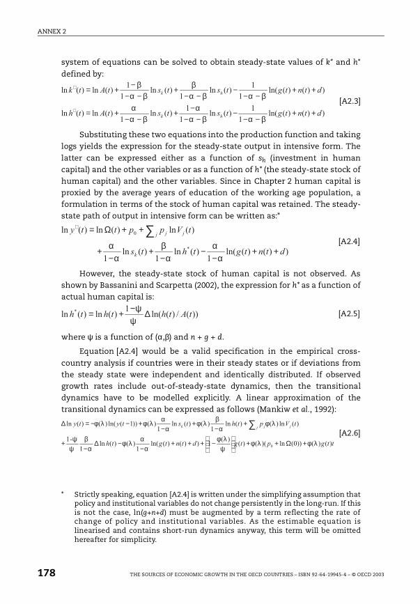
ANNEX 2
system of equations can be solved to obtain steady-state values of k* and h*
defined by:
Substituting these two equations into the production function and takinglogs yields the expression for the steady-state output in intensive form. The
latter can be expressed either as a function of sh (investment in humancapital) and the other variables or as a function of h* (the steady-state stock ofhuman capital) and the other variables. Since in Chapter 2 human capital isproxied by the average years of education of the working age population, aformulation in terms of the stock of human capital was retained. The steady-state path of output in intensive form can be written as:*
However, the steady-state stock of human capital is not observed. Asshown by Bassanini and Scarpetta (2002), the expression for h* as a function ofactual human capital is:
where ψ is a function of (α,β) and n + g + d.
Equation [A2.4] would be a valid specification in the empirical cross-
country analysis if countries were in their steady states or if deviations fromthe steady state were independent and identically distributed. If observedgrowth rates include out-of-steady-state dynamics, then the transitionaldynamics have to be modelled explicitly. A linear approximation of thetransitional dynamics can be expressed as follows (Mankiw et al., 1992):
* Strictly speaking, equation [A2.4] is written under the simplifying assumption thatpolicy and institutional variables do not change persistently in the long-run. If thisis not the case, ln(g+n+d) must be augmented by a term reflecting the rate ofchange of policy and institutional variables. As the estimable equation islinearised and contains short-run dynamics anyway, this term will be omittedhereafter for simplicity.
))()(ln(1
1)(ln
1
1)(ln
1)(ln)(ln
))()(ln(1
1)(ln
1)(ln
1
1)(ln)(ln
dtntgtststAth
dtntgtststAtk
hk
hk
++−−
−−−
−+−−
+=
++−−
−−−
+−−
−+=
∗
∗
βαβαα
βαα
βαβαβ
βαβ
[A2.3]
))()(ln(1
)(ln1
)(ln1
)(ln)(ln)(ln
*
0
dtntgthts
tVpptty
k
j jj
++−
−−
+−
+
++Ω= ∑∗
αα
αβ
αα [A2.4]
))(/)(ln(1
)(ln)(ln * tAththth ∆−+=ψ
ψ[A2.5]
ttgptgdtntgth
tVpthtstytyj jjk
)()())0(ln)(()()(
1))()(ln(1
)()(ln1
-1
)(ln)()(ln1
)()(ln1
)())1(ln()()(ln
0 λφλφψλφ
ααλφ
αβ
ψψ
λφα
βλφα
αλφλφ
+Ω++
−+++
−−∆
−+
+−
+−
+−−=∆ ∑[A2.6]
178 THE SOURCES OF ECONOMIC GROWTH IN THE OECD COUNTRIES – ISBN 92-64-19945-4 – © OECD 2003
ANNEX 2
where . Adding short-term dynamics to
equation [A2.6] yields:
Equation [A2.7] represents the generic functional form that has beenempirically estimated in Chapter 2. Estimates of steady state coefficients aswell as of the parameters of the production function can be retrieved on thebasis of the estimated coefficients of this equation by comparing it withequation [A2.6]. For instance, an estimate of the elasticity of steady stateoutput to the investment rate (that is the long-run effect of the investmentrate on output) is given by , where ^ identifies estimated coefficients.Conversely, an estimate of the share of physical capital in output (theparameter α of the production function) can be obtained as .
))()()(1( dtntg ++−−= βαλ
)(ln)(ln)(ln)(ln
ln)()(ln)(ln)1(ln)(ln
4321
443210
tVbtnbthbtsb
Vatatnathatsatyaty
j jjk
j jjk
ε
φ
+∆+∆+∆+∆+
++−++−−=∆
∑∑
+
+[A2.7]
φ/ˆ1a
)ˆˆ/(ˆ11 aa +φ
THE SOURCES OF ECONOMIC GROWTH IN THE OECD COUNTRIES – ISBN 92-64-19945-4 – © OECD 2003 179
ANNEX 3
Annex 3
Methodological details on the empirical analysis of industry multi-factor productivity1
A3.1. The theoretical framework
The basic framework of the analysis starts with a standard productionfunction (in country i and sector j), under perfect competition and constantreturns to scale. This can be formalised as follows:
where Y is output,2 A is a Hicks-neutral parameter of technical change,3 Fij isa country/sector-specific production function, K is physical capital and L
labour. Assuming a Cobb-Douglas production function and taking logs yield:
In this context, multi-factor productivity growth can be proxied by the socalled Solow residual as follows:
The convergence equation
In order to assess the driving forces of MFP growth, the models adopts acatch-up specification, whereby, within each industry, the productionpossibility set is influenced by technological and organisational transfer fromthe technology-frontier country to other countries. The co-integration modelof MFP may also account for the international transmission of business cyclesacross OECD countries (for instance trade and financial channels). In this
context, multi-factor productivity for a given industry j of country i at date t(MFPijt) can be modelled as an auto-regressive distributed lag ADL(1,1) processin which the level of MFP is co-integrated with the level of MFP of thetechnological frontier country F. Formally:
( )ijtijtijijtijt KLFAY ,⋅=
( ) ijtijtijtijtijtijt klay ⋅−+⋅+= αα 1
( ) ijtijtijtijtijtijt klyMFP ∆⋅−−∆⋅−∆=∆ αα 1
ijtFjtFjtijtijt MFPMFPMFPMFP ωβββ +++= −− 13211 lnlnlnln [A3.1]
180 THE SOURCES OF ECONOMIC GROWTH IN THE OECD COUNTRIES – ISBN 92-64-19945-4 – © OECD 2003
ANNEX 3
where ω stands for all observable and non-observable factors influencing
the level of MFP. Under the assumption of long-run homogeneity (1 – β1 = β2 +β3) and rearranging equation [A3.1] yields the convergence equation:
where RMFPijt = ln(MFPijt) – ln(MFPFjt) is the technological gap between countryi and the leading country F. This is the specification used in the empiricalanalysis. Moreover, the following (productivity) index is used as a measure of
the MFP level:
where a bar denotes a geometric average over all the countries for a given
industry j and year t. The index has the desirable properties of superlativenessand transitiveness which makes it possible to compare national productivitylevels (see Caves et al., 1982). However, the comparison of productivity levelsalso requires the conversion of underlying data into a common currency,while also taking into account differences in purchasing powers acrosscountries. These issues are discussed in the next section.
The residual in equation [A3.2] is modelled as follows:
where (Vijt) is a vector of covariates (e.g. product and labour marketregulations, human capital, or R&D) affecting the level of MFP; fi, gj, and dt arerespectively country, industry and year fixed effects. ε is an 2d shock.Moreover, equation [A3.2] can be solved for steady-state MFP in country i
relative to the frontier in industry j which gives insights on the effects of thesecountry and/or country-industry specific factors on the steady-state level ofMFP.
The steady-state equilibrium
At a steady-state equilibrium, the independent variables are constantover time (ωijt = ωij) and the multi-factor productivity in sector j grows at thesame constant rate in all countries: ∆lnMFPijt = ∆lnMFPFj.
For the ease of exposition, the residual in equation [A3.2] is redefined asfollows:
where ω’ and ω’’ correspond to the factors affecting the rate of growth of MFPrespectively, directly or through the diffusion of technology and organisational
( ) ijtijtFjtijt RMFPMFPMFP ωββ +−−∆=∆ 12 1lnln [A3.2]
ijtijt
ijt
jt
ijt
jt
jt
ijt
ijtK
K
L
L
Y
YMFP
αα −
⋅
⋅=
1
[A3.3]
∑ ++++= −k
ijttjikijtkijt dgfV εγω 1 [A3.4]
ijtijtijtijt RMFP⋅+= ''' ωωω [A3.5]
THE SOURCES OF ECONOMIC GROWTH IN THE OECD COUNTRIES – ISBN 92-64-19945-4 – © OECD 2003 181
ANNEX 3
practises. Solving for the steady-state, one can obtain the following expression
for the level of MFP in country i relative to the frontier in industry j:
Notes
1. For details on the method of estimation (approach followed, diagnostic tests,sensitivity analysis, etc.) see Scarpetta and Tressel (2002).
2. The analysis follows a value-added concept of output, which does not requiremeasures of intermediate consumption. This is the proper approach because theindustries that we use may have different levels of aggregation.
3. Technical change is “Hicks neutral”, or “output augmenting”, when it can berepresented as an outward shift of the production function that affects all factorsof production in the same proportion.
( )( ) ij
Fjij
ij
MFPRMFP
''1
1'
1
2
ωββω
−−∆−−
= [A3.6]
182 THE SOURCES OF ECONOMIC GROWTH IN THE OECD COUNTRIES – ISBN 92-64-19945-4 – © OECD 2003
ANNEX 4
Annex 4
Details on firm-level data
A4.1. The data and indicators of firm dynamics and survival
Raw data on firm dynamics and survival
The analysis of firm entry and exit and firm survival presented inChapter 4 is based on business registers (Canada, Denmark, France, Finland,
Netherlands, United Kingdom and United States) or social security databases(Germany and Italy). Data for Portugal are drawn from an employee-basedregister containing information on both establishments and firms.
The key features of these data on firm dynamics and survival are asfollows:
Unit of observation: Data used in the study refer to the firm as the unit ofreference, with the exception of Germany where data are only available withreference to establishments. More specifically, most of the data used conformto the following definition (Eurostat, 1995) “an organisational unit producing
goods or services which benefits from a certain degree of autonomy in decision-
making, especially for the allocation of its current resources”. Generally, this will beabove the establishment level. However, firms that have operating units in
multiple countries in the EU will have at least one unit counted in eachcountry. Of course, it may well be that the national boundaries that generate astatistical split-up of a firm, in fact split a firm in a “real” sense as well. Alsorelated to the unit of analysis is the issue of mergers and acquisitions. Only insome countries does the business register keep close track of suchorganisational changes within and between firms. In addition, ownershipstructures themselves may vary across countries because of taxconsiderations or other factors that influence how business activities areorganised within the structure of defined legal entities.
Size threshold: While some registers include even single-personbusinesses, others omit firms smaller than a certain size, usually in terms ofthe number of employees, but sometimes in terms of other measures such assales (as is the case in the data for France and Italy). Data used in this studyexclude single-person businesses. However, because smaller firms tend tohave more volatile firm dynamics, remaining differences in the threshold
THE SOURCES OF ECONOMIC GROWTH IN THE OECD COUNTRIES – ISBN 92-64-19945-4 – © OECD 2003 183
ANNEX 4
across different country datasets should be taken into account in the
international comparison.
Period of analysis: Data on firm dynamics and survival are compiled onan annual basis, covering varying time spans. The German, Danish andFinnish register data cover the longest time periods, while data for the othercountries are available for shorter periods of time or, although available forlonger periods, include significant breaks in definitions or coverage. In most of
the analysis presented in Chapter 4, data refer to the period 1989-94, whichguarantees the largest country coverage.
Sectoral coverage: Special efforts have been made to organise the data ina common industry classification (ISIC Rev.3, see Table A4.1) that matches theOECD STAN database. In the panel data constructed to generate thetabulations, firms were allocated to the STAN industry that most closely fitted
their operations over the complete time-span. Note that in countries wherethe data collection by the statistical agency varied across major sectors(e.g., construction, industry, services), a firm that switched between majorsectors could not be tracked as a continuing firm, but ended up creating anexit in one sector and an entry in another. Most countries have been able toprovide firm demographic data across most sectors of the economy, with theexception that public services are often not included (the United Kingdom is aspecial case, where data only refer only to manufacturing).
Indicators collected for firm dynamics and survival
The use of annual data on firm dynamics implies a significant volatilityin the resulting indicators. In order to limit the possible impact ofmeasurement problems, it was decided to use definitions of continuing,entering and exiting firms on the basis of three (rather than the usual two)time periods. Thus, the tabulations of firm dynamics contained the followingvariables:
Firm entry, comprising firms observed as (out, in, in) the register in time(t – 1, t, t + 1).
Firm exit, comprising firms observed as (in, in, out) the register in time(t – 1, t, t + 1).
Continuing firms, comprising firms observed as (in, in, in) the register intime (t – 1, t, t + 1).
One-year firms, comprising firms observed as (in, out, in) the register intime (t – 1, t, t + 1).
184 THE SOURCES OF ECONOMIC GROWTH IN THE OECD COUNTRIES – ISBN 92-64-19945-4 – © OECD 2003
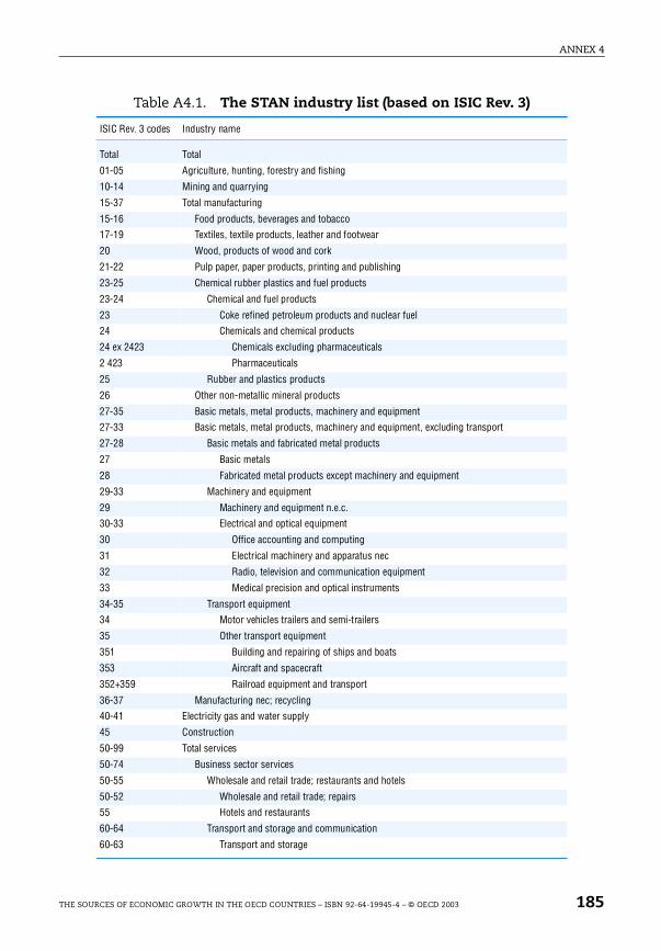
ANNEX 4
Table A4.1. The STAN industry list (based on ISIC Rev. 3)
ISIC Rev. 3 codes Industry name
Total Total
01-05 Agriculture, hunting, forestry and fishing
10-14 Mining and quarrying
15-37 Total manufacturing
15-16 Food products, beverages and tobacco
17-19 Textiles, textile products, leather and footwear
20 Wood, products of wood and cork
21-22 Pulp paper, paper products, printing and publishing
23-25 Chemical rubber plastics and fuel products
23-24 Chemical and fuel products
23 Coke refined petroleum products and nuclear fuel
24 Chemicals and chemical products
24 ex 2423 Chemicals excluding pharmaceuticals
2 423 Pharmaceuticals
25 Rubber and plastics products
26 Other non-metallic mineral products
27-35 Basic metals, metal products, machinery and equipment
27-33 Basic metals, metal products, machinery and equipment, excluding transport
27-28 Basic metals and fabricated metal products
27 Basic metals
28 Fabricated metal products except machinery and equipment
29-33 Machinery and equipment
29 Machinery and equipment n.e.c.
30-33 Electrical and optical equipment
30 Office accounting and computing
31 Electrical machinery and apparatus nec
32 Radio, television and communication equipment
33 Medical precision and optical instruments
34-35 Transport equipment
34 Motor vehicles trailers and semi-trailers
35 Other transport equipment
351 Building and repairing of ships and boats
353 Aircraft and spacecraft
352+359 Railroad equipment and transport
36-37 Manufacturing nec; recycling
40-41 Electricity gas and water supply
45 Construction
50-99 Total services
50-74 Business sector services
50-55 Wholesale and retail trade; restaurants and hotels
50-52 Wholesale and retail trade; repairs
55 Hotels and restaurants
60-64 Transport and storage and communication
60-63 Transport and storage
THE SOURCES OF ECONOMIC GROWTH IN THE OECD COUNTRIES – ISBN 92-64-19945-4 – © OECD 2003 185

ANNEX 4
This method of defining continuing, entering and exiting firms impliesthat a change in the stock of continuing firms (C) relates to entry (E) and exit(X) in the following way:
This has implications for the appropriate measure of firm “turnover”.Given that continuing, entering, exiting and “one-year” firms (O) all exist intime t then the total number of firms (T) is:
From this, the change in the total number of firms between two years,taking into account equation A4.1, can be written as:
Thus, a turnover measure that is consistent with the contribution of netentry to changes in the total number of firms should be based on the sum ofcontemporaneous entry with lagged exit.
In practice, a number of complications arise in constructing andinterpreting data that conform to the definitions of continuing, entering andexiting firms described above. In particular, the “one-year” category, in
Table A4.1. The STAN industry list (based on ISIC Rev. 3) (cont.)
Source: OECD.
ISIC Rev. 3 codes Industry name
64 Post and telecommunications
65-74 Finance insurance real estate and business services
65-67 Financial intermediation
65 Financial intermediation except insurance and pension funding
66 Insurance and pension funding except compulsory social security
67 Activities related to financial intermediation
70-74 Real estate renting and business activities
70 Real estate activities
71 Renting of machinery and equipment
72 Computer and related activities
73 Research and development
74 Other business activities
75-99 Community social and personal services
75 Public admin. and defence; compulsory social security
80 Education
85 Health and social work
90-93 Other community social and personal services
95 Private households with employed persons
99 Extra-territorial organisations and bodies
tttt XECC −=− −− 11[A4.1]
ttttt OXECT +++= [A4.2]
111 −−− −+−=− tttttt OOXETT [A4.3]
186 THE SOURCES OF ECONOMIC GROWTH IN THE OECD COUNTRIES – ISBN 92-64-19945-4 – © OECD 2003
ANNEX 4
principle, represents short-lived firms that are observed in time t but not in
adjacent time periods and could therefore be treated as an additional piece ofinformation in evaluating firm demographics. However, in some databasesthis category also includes measurement errors and possibly ill-defined data.Thus, the total number of firms in the analysis for the main text excludesthese “one-year” firms.
Available data also allowed to track entering firms over time and to assess
the contribution of firm dynamics to the overall job turnover by industry andover time. In particular, the following indicators were constructed:
The analysis of survival: Entering cohorts of firms were tracked downwhich allowed assessment of the probability of failure and survivor rates byduration. Moreover, information was collected on employment in thesefirms, both in the year of entry and in subsequent years.
Job creation and destruction: Additional information on employmentchanges in continuing firms also permitted the calculation of the overall jobturnover by industry and over time and assessment of the contribution offirm dynamics to this process.1
A4.2. Productivity decomposition data
Using mainly longitudinal business surveys, Chapter 4 provides adecomposition of industry productivity growth into the contribution ofwithin-firm growth and that due to reallocation of resources across firms –which includes reallocation amongst incumbents, as well as reallocation due
to the entry of new units and/or the exit of other units. Detailed results arepresented in Tables A4.2 to A4.8 at the end of this Annex. They are based on
the approach developed by Griliches and Regev (1995) (referred to hereafter asthe GR method), but alternative calculations were also made in order to checkthe robustness of the results, based on the method developed by Foster,Haltiwanger, and Krizan (1998) (referred hereafter as the FHK method). Thissection of the Annex aims to provide methodological details on bothapproaches. Full details on their results can be found in Scarpetta et al. (2002).
Definition of entry and exit
Following standard practice, the productivity decompositions were basedon a fairly long time interval (in this case 5 years). Thus, unlike the annualfirm-demographics data, a more conventional method of defining continuing,entering and exiting firms was used:
Continuing firms: observed both in the first year (t – k) and the last year (t)of the period.
THE SOURCES OF ECONOMIC GROWTH IN THE OECD COUNTRIES – ISBN 92-64-19945-4 – © OECD 2003 187
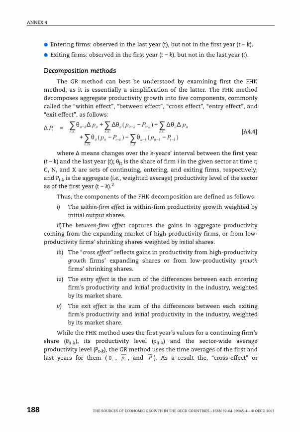
ANNEX 4
Entering firms: observed in the last year (t), but not in the first year (t – k).
Exiting firms: observed in the first year (t − k), but not in the last year (t).
Decomposition methods
The GR method can best be understood by examining first the FHKmethod, as it is essentially a simplification of the latter. The FHK methoddecomposes aggregate productivity growth into five components, commonlycalled the “within effect”, “between effect”, “cross effect”, “entry effect”, and“exit effect”, as follows:
where ∆ means changes over the k-years’ interval between the first year(t − k) and the last year (t); θit is the share of firm i in the given sector at time t;C, N, and X are sets of continuing, entering, and exiting firms, respectively;and Pt-k is the aggregate (i.e., weighted average) productivity level of the sectoras of the first year (t − k).2
Thus, the components of the FHK decomposition are defined as follows:
i) The within-firm effect is within-firm productivity growth weighted byinitial output shares.
ii)The between-firm effect captures the gains in aggregate productivitycoming from the expanding market of high productivity firms, or from low-productivity firms’ shrinking shares weighted by initial shares.
iii) The “cross effect” reflects gains in productivity from high-productivitygrowth firms’ expanding shares or from low-productivity growth
firms’ shrinking shares.
iv) The entry effect is the sum of the differences between each enteringfirm’s productivity and initial productivity in the industry, weightedby its market share.
v) The exit effect is the sum of the differences between each exitingfirm’s productivity and initial productivity in the industry, weightedby its market share.
While the FHK method uses the first year’s values for a continuing firm’sshare (θit-k), its productivity level (pit-k) and the sector-wide average
productivity level (Pt-k), the GR method uses the time averages of the first andlast years for them ( , , and ). As a result the, “cross-effect” or
)()(
)(
ktkit
Xi
kitktit
Ni
it
Ci
ititkt
Ci
kititit
Ci
kitt
PpPp
pPppP
−−∈
−−∈
∈−
∈−
∈−
−−−+
∆∆+−∆+∆=∆
∑∑∑∑∑
θθ
θθθ[A4.4]
iθ ip P
188 THE SOURCES OF ECONOMIC GROWTH IN THE OECD COUNTRIES – ISBN 92-64-19945-4 – © OECD 2003
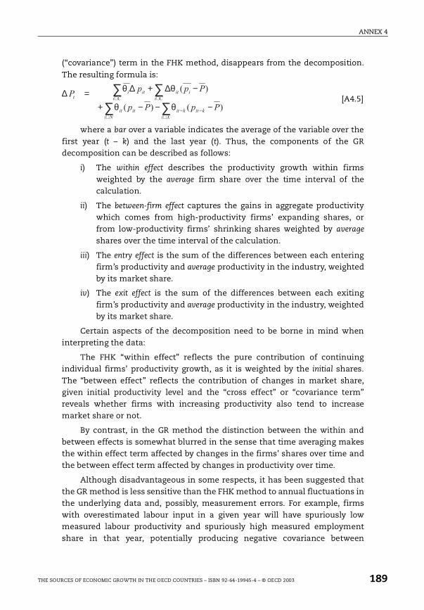
ANNEX 4
(“covariance”) term in the FHK method, disappears from the decomposition.
The resulting formula is:
where a bar over a variable indicates the average of the variable over thefirst year (t – k) and the last year (t). Thus, the components of the GRdecomposition can be described as follows:
i) The within effect describes the productivity growth within firmsweighted by the average firm share over the time interval of thecalculation.
ii) The between-firm effect captures the gains in aggregate productivitywhich comes from high-productivity firms’ expanding shares, orfrom low-productivity firms’ shrinking shares weighted by average
shares over the time interval of the calculation.
iii) The entry effect is the sum of the differences between each enteringfirm’s productivity and average productivity in the industry, weightedby its market share.
iv) The exit effect is the sum of the differences between each exitingfirm’s productivity and average productivity in the industry, weightedby its market share.
Certain aspects of the decomposition need to be borne in mind wheninterpreting the data:
The FHK “within effect” reflects the pure contribution of continuingindividual firms’ productivity growth, as it is weighted by the initial shares.The “between effect” reflects the contribution of changes in market share,given initial productivity level and the “cross effect” or “covariance term”reveals whether firms with increasing productivity also tend to increasemarket share or not.
By contrast, in the GR method the distinction between the within andbetween effects is somewhat blurred in the sense that time averaging makesthe within effect term affected by changes in the firms’ shares over time andthe between effect term affected by changes in productivity over time.
Although disadvantageous in some respects, it has been suggested thatthe GR method is less sensitive than the FHK method to annual fluctuations inthe underlying data and, possibly, measurement errors. For example, firmswith overestimated labour input in a given year will have spuriously lowmeasured labour productivity and spuriously high measured employmentshare in that year, potentially producing negative covariance between
)()(
)(
PpPp
PppP
kit
Xi
kitit
Ni
it
Ci
iitit
Ci
it
−−−+
−∆+∆=∆
−∈
−∈
∈∈
∑∑∑∑
θθ
θθ[A4.5]
THE SOURCES OF ECONOMIC GROWTH IN THE OECD COUNTRIES – ISBN 92-64-19945-4 – © OECD 2003 189

ANNEX 4
productivity and share changes. In this case, the within effect in the FHK
method could be misleadingly high.3
Care has to be taken in interpreting the entry and exit components asthey do not always reflect a comparison between productivity levels at thesame point in time. For example, in the version of the FHK decompositionused in Chapter 4, the entry component comprises the difference betweenaverage productivity among entrants at the end of the 5-year period with
overall productivity at the beginning. Obviously, therefore, a positive entrycomponent does not necessarily mean that productivity among entering firmsis above average in relation to their contemporaries.
Notes
1. It should be noted that the gross employment flows tabulated from the statisticalregister files do not necessarily coincide with gross job flow data tabulated fromproduction surveys, such as those used by Davis et al. (1996).
2. The shares are usually based on employment in decompositions of labourproductivity and on output in decompositions of total factor productivity.
3. Similarly, in the case of total factor productivity decomposition using outputshares, random measurement errors in output could yield a positive covariancebetween productivity changes and share changes, and hence, the within effectcould be spuriously low.
190 THE SOURCES OF ECONOMIC GROWTH IN THE OECD COUNTRIES – ISBN 92-64-19945-4 – © OECD 2003
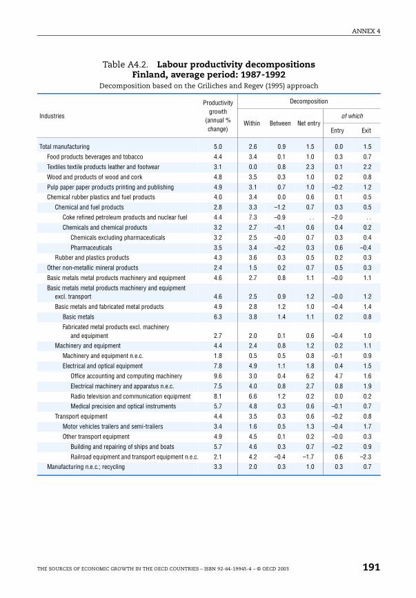
ANNEX 4
it
.5
.7
.2
.8
.2
.5
.5
. .
.2
.4
.4
.3
.3
.1
.2
.4
.8
.0
.1
.9
.5
.6
.9
.2
.7
.8
.7
.3
.9
.3
.7
Table A4.2. Labour productivity decompositions Finland, average period: 1987-1992
Decomposition based on the Griliches and Regev (1995) approach
Industries
Productivity growth
(annual % change)
Decomposition
Within Between Net entryof which
Entry Ex
Total manufacturing 5.0 2.6 0.9 1.5 0.0 1
Food products beverages and tobacco 4.4 3.4 0.1 1.0 0.3 0
Textiles textile products leather and footwear 3.1 0.0 0.8 2.3 0.1 2
Wood and products of wood and cork 4.8 3.5 0.3 1.0 0.2 0
Pulp paper paper products printing and publishing 4.9 3.1 0.7 1.0 –0.2 1
Chemical rubber plastics and fuel products 4.0 3.4 0.0 0.6 0.1 0
Chemical and fuel products 2.8 3.3 –1.2 0.7 0.3 0
Coke refined petroleum products and nuclear fuel 4.4 7.3 –0.9 . . –2.0
Chemicals and chemical products 3.2 2.7 –0.1 0.6 0.4 0
Chemicals excluding pharmaceuticals 3.2 2.5 –0.0 0.7 0.3 0
Pharmaceuticals 3.5 3.4 –0.2 0.3 0.6 –0
Rubber and plastics products 4.3 3.6 0.3 0.5 0.2 0
Other non-metallic mineral products 2.4 1.5 0.2 0.7 0.5 0
Basic metals metal products machinery and equipment 4.6 2.7 0.8 1.1 –0.0 1
Basic metals metal products machinery and equipment excl. transport 4.6 2.5 0.9 1.2 –0.0 1
Basic metals and fabricated metal products 4.9 2.8 1.2 1.0 –0.4 1
Basic metals 6.3 3.8 1.4 1.1 0.2 0
Fabricated metal products excl. machinery and equipment 2.7 2.0 0.1 0.6 –0.4 1
Machinery and equipment 4.4 2.4 0.8 1.2 0.2 1
Machinery and equipment n.e.c. 1.8 0.5 0.5 0.8 –0.1 0
Electrical and optical equipment 7.8 4.9 1.1 1.8 0.4 1
Office accounting and computing machinery 9.6 3.0 0.4 6.2 4.7 1
Electrical machinery and apparatus n.e.c. 7.5 4.0 0.8 2.7 0.8 1
Radio television and communication equipment 8.1 6.6 1.2 0.2 0.0 0
Medical precision and optical instruments 5.7 4.8 0.3 0.6 –0.1 0
Transport equipment 4.4 3.5 0.3 0.6 –0.2 0
Motor vehicles trailers and semi-trailers 3.4 1.6 0.5 1.3 –0.4 1
Other transport equipment 4.9 4.5 0.1 0.2 –0.0 0
Building and repairing of ships and boats 5.7 4.6 0.3 0.7 –0.2 0
Railroad equipment and transport equipment n.e.c. 2.1 4.2 –0.4 –1.7 0.6 –2
Manufacturing n.e.c.; recycling 3.3 2.0 0.3 1.0 0.3 0
THE SOURCES OF ECONOMIC GROWTH IN THE OECD COUNTRIES – ISBN 92-64-19945-4 – © OECD 2003 191
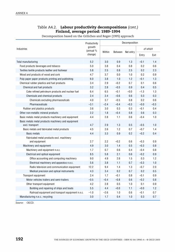
ANNEX 4
it
.4
.6
.3
.9
.3
.6
.5
.3
.3
.6
.3
.4
.3
.0
.0
.4
.4
.9
.8
.8
.9
.2
.0
.0
.5
.9
.8
.9
.2
.7
.7
Table A4.2. Labour productivity decompositions (cont.)Finland, average period: 1989-1994
Decomposition based on the Griliches and Regev (1995) approach
Source: OECD.
Industries
Productivity growth
(annual % change)
Decomposition
Within Between Net entryof which
Entry Ex
Total manufacturing 5.2 3.0 0.9 1.3 –0.1 1
Food products beverages and tobacco 5.0 3.8 0.4 0.8 0.2 0
Textiles textile products leather and footwear 5.8 2.5 0.8 2.5 0.2 2
Wood and products of wood and cork 4.7 3.7 0.0 1.0 0.2 0
Pulp paper paper products printing and publishing 6.0 3.8 1.0 1.2 –0.1 1
Chemical rubber plastics and fuel products 3.4 2.9 –0.2 0.7 0.1 0
Chemical and fuel products 3.2 2.8 –0.5 0.9 0.4 0
Coke refined petroleum products and nuclear fuel 6.4 6.5 –0.1 –0.0 –1.3 1
Chemicals and chemical products 2.4 2.4 –0.6 0.6 0.3 0
Chemicals excluding pharmaceuticals 4.0 3.7 –0.5 0.8 0.2 0
Pharmaceuticals –3.1 –2.4 –0.4 –0.3 –0.0 –0
Rubber and plastics products 3.6 3.0 0.3 0.3 –0.1 0
Other non-metallic mineral products 2.2 1.8 –0.4 0.8 0.6 0
Basic metals metal products machinery and equipment 4.4 2.8 1.1 0.6 –0.4 1
Basic metals metal products machinery and equipment excl. transport 4.7 2.9 1.3 0.5 –0.5 1
Basic metals and fabricated metal products 4.5 2.6 1.2 0.7 –0.7 1
Basic metals 4.4 3.3 0.9 0.2 –0.2 0
Fabricated metal products excl. machinery and equipment 2.7 2.2 –0.2 0.6 –0.3 0
Machinery and equipment 4.9 3.0 1.4 0.5 –0.3 0
Machinery and equipment n.e.c. 1.7 0.7 0.6 0.4 –0.4 0
Electrical and optical equipment 8.5 5.8 2.1 0.6 –0.2 0
Office accounting and computing machinery 9.0 4.9 2.6 1.5 0.3 1
Electrical machinery and apparatus n.e.c. 5.6 3.8 1.1 0.7 –0.3 1
Radio television and communication equipment 12.2 9.4 1.4 1.3 –0.7 2
Medical precision and optical instruments 4.3 3.4 0.2 0.7 0.2 0
Transport equipment 2.4 1.7 –0.1 0.8 –0.1 0
Motor vehicles trailers and semi-trailers –0.5 –0.4 –0.8 0.6 –0.2 0
Other transport equipment 4.2 2.8 0.5 1.0 0.1 0
Building and repairing of ships and boats 5.5 4.4 –0.0 1.1 –0.0 1
Railroad equipment and transport equipment n.e.c. –1.0 –2.6 1.0 0.6 –0.1 0
Manufacturing n.e.c.; recycling 3.0 1.7 0.4 1.0 0.3 0
192 THE SOURCES OF ECONOMIC GROWTH IN THE OECD COUNTRIES – ISBN 92-64-19945-4 – © OECD 2003
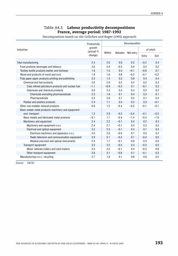
ANNEX 4
it
.4
.2
.7
.2
.4
.3
.2
.2
.1
.4
.1
.1
.3
.0
.3
.2
.3
.2
.5
.6
.5
.6
.2
.2
Table A4.3. Labour productivity decompositions France, average period: 1987-1992
Decomposition based on the Griliches and Regev (1995) approach
Source: OECD.
Industries
Productivity growth
(annual % change)
Decomposition
Within Between Net entryof which
Entry Ex
Total manufacturing 2.3 2.0 0.0 0.2 –0.2 0Food products beverages and tobacco 2.6 2.4 –0.3 0.4 0.2 0Textiles textile products leather and footwear 1.8 1.5 0.3 –0.1 –0.8 0Wood and products of wood and cork 1.9 1.6 0.6 –0.3 –0.1 –0Pulp paper paper products printing and publishing 2.3 1.3 0.2 0.8 0.4 0
Chemical and fuel products 2.6 2.0 0.2 0.4 0.2 0Coke refined petroleum products and nuclear fuel –1.1 –0.9 –0.3 0.1 –0.1 0Chemicals and chemical products 3.0 2.3 0.3 0.4 0.2 0
Chemicals excluding pharmaceuticals 2.3 1.9 0.1 0.4 0.3 0Pharmaceuticals 4.2 3.0 0.7 0.5 0.1 0
Rubber and plastics products 2.4 1.7 0.5 0.2 0.3 –0Other non-metallic mineral products 0.6 1.2 –0.4 –0.2 –0.1 –0Basic metals metal products machinery and equipment
excl. transport 1.3 2.0 –0.2 –0.4 –0.1 –0Basic metals and fabricated metal products –0.1 1.7 –0.4 –1.4 –0.4 –1Machinery and equipment 2.4 2.2 –0.1 0.4 0.2 0
Machinery and equipment n.e.c. 2.4 2.1 –0.1 0.4 0.2 0Electrical and optical equipment 2.5 2.3 –0.1 0.4 0.1 0
Electrical machinery and apparatus n.e.c. 2.6 2.0 –0.0 0.7 0.5 0Radio television and communication equipment 2.9 3.1 –0.3 0.1 –0.4 0Medical precision and optical instruments 2.4 1.7 –0.1 0.9 0.3 0
Transport equipment 3.2 3.2 –0.3 0.3 –0.3 0Motor vehicles trailers and semi-trailers 3.5 3.2 –0.1 0.4 –0.3 0Other transport equipment 2.6 3.1 –0.6 0.1 –0.1 0
Manufacturing n.e.c.; recycling 2.7 1.8 0.1 0.8 0.6 0
THE SOURCES OF ECONOMIC GROWTH IN THE OECD COUNTRIES – ISBN 92-64-19945-4 – © OECD 2003 193
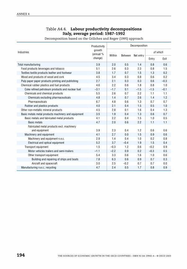
ANNEX 4
it
.6
.5
.2
.2
.3
.0
.1
.1
.2
.7
.0
.3
.7
.5
.1
.6
.6
.8
.4
.9
.5
.6
.3
.0
.9
Table A4.4. Labour productivity decompositions Italy, average period: 1987-1992
Decomposition based on the Griliches and Regev (1995) approach
Industries
Productivity growth
(annual % change)
Decomposition
Within Between Net entryof which
Entry Ex
Total manufacturing 3.9 2.0 0.5 1.4 0.8 0Food products beverages and tobacco 5.1 2.6 0.3 2.3 0.8 1Textiles textile products leather and footwear 3.8 1.7 0.7 1.5 1.3 0Wood and products of wood and cork 4.5 3.4 0.3 0.8 0.6 0Pulp paper paper products printing and publishing 2.7 2.1 0.3 0.3 0.6 –0Chemical rubber plastics and fuel products 4.6 2.2 0.6 1.8 0.8 1
Coke refined petroleum products and nuclear fuel –3.1 –1.7 0.1 –1.5 –1.5 –0Chemicals and chemical products 5.5 2.6 0.7 2.2 1.1 1
Chemicals excluding pharmaceuticals 4.8 1.4 0.7 2.6 1.4 1Pharmaceuticals 6.7 4.8 0.6 1.3 0.7 0
Rubber and plastics products 4.0 2.1 0.4 1.5 0.5 1Other non-metallic mineral products 4.5 2.8 0.1 1.6 0.4 1Basic metals metal products machinery and equipment 3.5 1.9 0.4 1.3 0.6 0
Basic metals and fabricated metal products 4.1 2.2 0.4 1.5 1.0 0Basic metals 4.7 2.0 0.6 2.2 1.1 1Fabricated metal products excl. machinery
and equipment 3.9 2.3 0.4 1.2 0.6 0Machinery and equipment 4.1 2.7 0.0 1.5 0.9 0
Machinery and equipment n.e.c. 2.9 1.4 0.4 1.0 0.2 0Electrical and optical equipment 5.2 3.7 –0.4 1.9 1.5 0
Transport equipment 1.5 –0.3 1.2 0.6 –0.2 0Motor vehicles trailers and semi-trailers –1.1 –2.2 0.9 0.2 –0.3 0Other transport equipment 5.4 3.3 0.6 1.6 1.0 0
Building and repairing of ships and boats 7.8 6.3 0.6 0.9 0.7 0Aircraft and spacecraft 3.0 2.5 –0.2 0.7 0.7 0
Manufacturing n.e.c.; recycling 4.7 2.4 0.5 1.7 0.8 0
194 THE SOURCES OF ECONOMIC GROWTH IN THE OECD COUNTRIES – ISBN 92-64-19945-4 – © OECD 2003
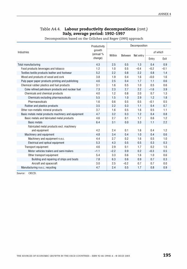
ANNEX 4
it
.9
.1
.4
.6
.6
.6
.9
.3
.8
.5
.7
.1
.8
.2
.2
.2
.6
.0
.3
.5
.5
.6
.3
.0
.9
Table A4.4. Labour productivity decompositions (cont.)Italy, average period: 1992-1997
Decomposition based on the Griliches and Regev (1995) approach
Source: OECD.
Industries
Productivity growth
(annual % change)
Decomposition
Within Between Net entryof which
Entry Ex
Total manufacturing 4.3 2.5 0.5 1.3 0.4 0Food products beverages and tobacco 1.2 1.0 0.5 –0.4 –0.2 –0Textiles textile products leather and footwear 5.2 2.2 0.8 2.2 0.8 1Wood and products of wood and cork 3.8 1.9 0.4 1.6 –0.0 1Pulp paper paper products printing and publishing 4.6 2.5 0.4 1.7 1.1 0Chemical rubber plastics and fuel products 3.1 1.6 0.5 1.0 0.5 0
Coke refined petroleum products and nuclear fuel 7.3 2.3 2.7 2.2 –1.6 3Chemicals and chemical products 4.0 1.2 0.8 2.0 0.7 1
Chemicals excluding pharmaceuticals 5.5 1.5 1.0 2.9 1.2 1Pharmaceuticals 1.6 0.6 0.5 0.5 –0.1 0
Rubber and plastics products 3.5 2.2 0.3 1.1 0.4 0Other non-metallic mineral products 3.7 1.6 0.5 1.6 0.5 1Basic metals metal products machinery and equipment 4.7 3.2 0.3 1.2 0.4 0
Basic metals and fabricated metal products 4.6 2.7 0.1 1.7 0.6 1Basic metals 6.4 3.1 0.0 3.3 1.1 2Fabricated metal products excl. machinery
and equipment 4.2 2.4 0.1 1.6 0.4 1Machinery and equipment 4.8 3.4 0.4 1.0 0.4 0
Machinery and equipment n.e.c. 4.4 2.7 0.2 1.6 0.5 1Electrical and optical equipment 5.3 4.3 0.5 0.5 0.3 0
Transport equipment 4.6 2.9 0.1 1.7 0.2 1Motor vehicles trailers and semi-trailers –1.1 –2.2 0.9 0.2 –0.3 0Other transport equipment 5.4 3.3 0.6 1.6 1.0 0
Building and repairing of ships and boats 7.8 6.3 0.6 0.9 0.7 0Aircraft and spacecraft 3.0 2.5 –0.2 0.7 0.7 0
Manufacturing n.e.c.; recycling 4.7 2.4 0.5 1.7 0.8 0
THE SOURCES OF ECONOMIC GROWTH IN THE OECD COUNTRIES – ISBN 92-64-19945-4 – © OECD 2003 195
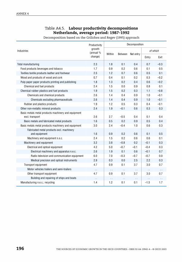
ANNEX 4
it
.3
.5
.1
.2
.2
.1
.8
.1
.1
.1
.3
.4
.4
.3
.5
.1
.3
.3
.7
.0
.3
.7
. .
.7
. .
.7
Table A4.5. Labour productivity decompositionsNetherlands, average period: 1987-1992
Decomposition based on the Griliches and Regev (1995) approach
Industries
Productivity growth
(annual % change)
Decomposition
Within Between Net entryof which
Entry Ex
Total manufacturing 2.3 1.8 0.1 0.4 0.7 –0
Food products beverages and tobacco 1.7 0.9 0.2 0.6 0.1 0
Textiles textile products leather and footwear 2.5 1.2 0.7 0.6 0.5 0
Wood and products of wood and cork 0.7 0.4 0.1 0.2 0.3 –0
Pulp paper paper products printing and publishing 1.8 1.3 0.2 0.4 0.6 –0
Chemical and fuel products 2.4 1.5 0.0 0.9 0.8 0
Chemical rubber plastics and fuel products 1.9 1.5 0.2 0.3 1.1 –0
Chemicals and chemical products 2.6 1.4 0.4 0.9 1.0 –0
Chemicals excluding pharmaceuticals 2.6 1.4 0.4 0.9 1.0 –0
Rubber and plastics products 1.9 1.2 0.5 0.3 0.4 –0
Other non-metallic mineral products 2.4 1.9 –0.1 0.6 0.3 0
Basic metals metal products machinery and equipment excl. transport 2.6 2.7 –0.5 0.4 0.1 0
Basic metals and fabricated metal products 1.6 0.5 0.2 0.9 0.5 0
Basic metals metal products machinery and equipment 3.0 2.4 –0.4 1.0 0.6 0
Fabricated metal products excl. machinery and equipment 1.6 0.9 0.2 0.6 0.1 0
Machinery and equipment n.e.c. 2.4 1.5 0.2 0.6 0.6 0
Machinery and equipment 3.2 3.8 –0.8 0.2 –0.1 0
Electrical and optical equipment 4.2 5.0 –0.7 –0.1 –0.4 0
Electrical machinery and apparatus n.e.c. 2.6 1.9 0.1 0.6 –0.1 0
Radio television and communication equipment 6.0 7.0 –0.3 –0.7 –0.7 0
Medical precision and optical instruments 2.9 0.3 0.0 2.5 2.2 0
Transport equipment 4.7 0.9 0.1 3.7 3.0 0
Motor vehicles trailers and semi-trailers . . . . . . . . . .
Other transport equipment 4.7 0.9 0.1 3.7 3.0 0
Building and repairing of ships and boats . . . . . . . . . .
Manufacturing n.e.c.; recycling 1.4 1.2 0.1 0.1 –1.5 1
196 THE SOURCES OF ECONOMIC GROWTH IN THE OECD COUNTRIES – ISBN 92-64-19945-4 – © OECD 2003
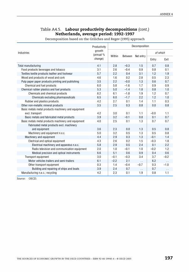
ANNEX 4
it
.8
.1
.9
.3
.7
.9
.0
.7
.0
.3
.8
.1
.7
.7
.8
.8
.4
.8
.2
.2
.6
.2
. .
.0
. .
.1
Table A4.5. Labour productivity decompositions (cont.)Netherlands, average period: 1992-1997
Decomposition based on the Griliches and Regev (1995) approach
Source: OECD.
Industries
Productivity growth
(annual % change)
Decomposition
Within Between Net entryof which
Entry Ex
Total manufacturing 4.1 2.8 –0.3 1.5 0.7 0Food products beverages and tobacco 3.1 2.6 –0.4 0.9 0.8 0Textiles textile products leather and footwear 5.7 2.2 0.4 3.1 1.2 1Wood and products of wood and cork 4.6 1.6 0.2 2.8 0.5 2Pulp paper paper products printing and publishing 3.5 2.2 –0.0 1.3 0.6 0
Chemical and fuel products 6.0 5.8 –1.6 1.7 0.9 0Chemical rubber plastics and fuel products 5.3 5.0 –1.4 1.8 0.8 1
Chemicals and chemical products 6.2 6.1 –1.8 1.9 1.2 0Chemicals excluding pharmaceuticals 6.5 6.0 –1.7 2.2 1.2 1
Rubber and plastics products 4.2 2.7 0.1 1.4 1.1 0Other non-metallic mineral products 3.5 2.5 0.3 0.8 0.0 0Basic metals metal products machinery and equipment
excl. transport 4.2 3.0 0.1 1.1 –0.0 1Basic metals and fabricated metal products 3.9 3.2 –0.1 0.8 0.1 0
Basic metals metal products machinery and equipment 4.0 2.5 0.1 1.3 0.7 0Fabricated metal products excl. machinery
and equipment 3.6 2.3 0.0 1.3 0.5 0Machinery and equipment n.e.c. 5.0 3.2 0.5 1.3 0.5 0
Machinery and equipment 4.4 2.9 0.3 1.3 –0.1 1Electrical and optical equipment 4.3 2.6 0.2 1.5 –0.3 1
Electrical machinery and apparatus n.e.c. 5.8 2.9 0.5 2.4 0.1 2Radio television and communication equipment 2.0 1.0 –0.1 1.0 –0.2 1Medical precision and optical instruments 6.6 5.1 0.6 0.9 0.4 0
Transport equipment 3.0 –0.1 –0.3 3.4 3.7 –0Motor vehicles trailers and semi-trailers 6.1 –2.2 2.1 . . 6.2Other transport equipment 0.3 1.4 –0.4 –0.7 0.3 –1
Building and repairing of ships and boats 3.9 2.4 0.7 . . 0.7Manufacturing n.e.c.; recycling 4.2 2.3 0.1 1.9 0.8 1
THE SOURCES OF ECONOMIC GROWTH IN THE OECD COUNTRIES – ISBN 92-64-19945-4 – © OECD 2003 197
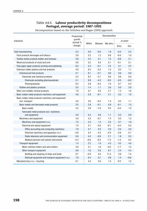
ANNEX 4
it
.2
.0
.1
.1
.2
.1
.0
.0
.0
.4
.0
.6
.9
.1
.0
.0
.9
.2
.8
.3
.6
.7
.3
.2
.0
.5
.3
.4
.6
.5
Table A4.6. Labour productivity decompositions Portugal, average period: 1987-1992
Decomposition based on the Griliches and Regev (1995) approach
Industries
Productivity growth
(annual % change)
Decomposition
Within Between Net entryof which
Entry Ex
Total manufacturing 5.3 4.0 –0.5 1.8 –0.4 2
Food products beverages and tobacco 3.9 2.2 1.2 0.6 –0.5 1
Textiles textile products leather and footwear 5.8 4.2 0.1 1.5 –0.6 2
Wood and products of wood and cork 5.6 3.2 0.4 2.1 –0.1 2
Pulp paper paper products printing and publishing 6.3 4.2 –0.1 2.2 0.1 2
Chemical rubber plastics and fuel products 4.6 6.3 –3.3 1.5 0.5 1
Chemical and fuel products 5.1 8.1 –3.7 0.6 0.6 0
Chemicals and chemical products 5.2 8.2 –3.7 0.6 0.6 0
Chemicals excluding pharmaceuticals 5.1 9.9 –4.3 –0.5 –0.5 –0
Pharmaceuticals 6.4 5.8 –0.4 1.0 0.7 0
Rubber and plastics products 5.5 1.4 1.1 3.0 0.0 3
Other non-metallic mineral products 7.9 4.7 0.5 2.7 1.2 1
Basic metals metal products machinery and equipment 4.8 2.9 –0.1 2.1 0.2 1
Basic metals metal products machinery and equipment excl. transport 4.0 3.0 –0.3 1.4 0.2 1
Basic metals and fabricated metal products 3.5 2.8 –0.1 0.9 –0.1 1
Basic metals 3.5 3.9 –1.0 0.5 –0.4 1
Fabricated metal products excl. machinery and equipment 4.0 2.4 0.6 1.1 0.2 0
Machinery and equipment 4.0 3.3 –0.7 1.4 0.3 1
Machinery and equipment n.e.c. 7.0 3.3 1.2 2.5 0.7 1
Electrical and optical equipment 1.0 3.7 –2.6 –0.1 –0.4 0
Office accounting and computing machinery 7.9 4.7 0.2 3.0 0.4 2
Electrical machinery and apparatus n.e.c. –3.8 3.4 –4.3 –2.9 –3.6 0
Radio television and communication equipment 5.6 4.4 –0.9 2.1 1.8 0
Medical precision and optical instruments –2.3 –0.6 –0.3 –1.3 –1.5 0
Transport equipment 7.4 2.2 1.0 4.3 0.2 4
Motor vehicles trailers and semi-trailers 3.9 3.1 1.0 –0.2 –1.7 1
Other transport equipment 8.8 1.6 0.5 6.7 2.4 4
Building and repairing of ships and boats 9.7 –2.0 0.4 11.3 3.9 7
Railroad equipment and transport equipment n.e.c. 7.8 6.4 0.7 0.8 1.4 –0
Manufacturing n.e.c.; recycling 6.1 4.4 0.3 1.4 –0.2 1
198 THE SOURCES OF ECONOMIC GROWTH IN THE OECD COUNTRIES – ISBN 92-64-19945-4 – © OECD 2003
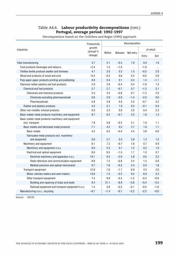
ANNEX 4
it
.9
. .
.0
.8
.1
.3
.1
.0
.6
.2
.4
.2
.4
.1
.1
.6
.5
.9
.0
.7
.2
.8
.8
.6
.2
.9
.5
.6
.0
Table A4.6. Labour productivity decompositions (cont.)Portugal, average period: 1992-1997
Decomposition based on the Griliches and Regev (1995) approach
Source: OECD.
Industries
Productivity growth
(annual % change)
Decomposition
Within Between Net entryof which
Entry Ex
Total manufacturing 4.7 3.1 –0.3 1.9 0.0 1
Food products beverages and tobacco –2.4 1.3 –1.9 . . –1.8
Textiles textile products leather and footwear 4.7 3.0 0.2 1.5 –0.5 2
Wood and products of wood and cork –0.4 –3.3 0.6 2.4 –0.5 2
Pulp paper paper products printing and publishing 0.8 0.4 0.1 0.3 1.4 –1
Chemical rubber plastics and fuel products 2.9 2.9 –0.4 0.4 –1.0 1
Chemical and fuel products 2.7 2.7 –0.7 0.7 –1.3 2
Chemicals and chemical products 3.4 3.4 –0.8 0.7 –1.3 2
Chemicals excluding pharmaceuticals 0.6 2.9 –0.9 –1.4 –2.0 0
Pharmaceuticals 5.8 2.8 0.5 2.5 –0.7 3
Rubber and plastics products 4.3 3.1 1.0 0.3 –0.1 0
Other non-metallic mineral products 6.0 3.3 0.0 2.6 0.4 2
Basic metals metal products machinery and equipment 8.7 6.2 –0.7 3.2 1.8 1
Basic metals metal products machinery and equipment excl. transport 7.9 5.9 –0.2 2.1 1.0 1
Basic metals and fabricated metal products 7.1 4.2 0.2 2.7 1.6 1
Basic metals 4.2 0.2 –0.4 4.4 3.8 0
Fabricated metal products excl. machinery and equipment 8.8 5.7 0.3 2.8 1.3 1
Machinery and equipment 8.1 7.2 –0.7 1.6 0.7 0
Machinery and equipment n.e.c. 6.6 5.3 0.1 1.2 0.2 1
Electrical and optical equipment 8.6 8.5 –1.5 1.7 1.0 0
Electrical machinery and apparatus n.e.c. 10.1 9.3 –2.0 2.8 0.5 2
Radio television and communication equipment 8.8 7.2 –0.8 2.4 1.5 0
Medical precision and optical instruments 9.7 7.6 –0.3 2.4 0.5 1
Transport equipment 12.8 7.6 –1.7 6.9 4.3 2
Motor vehicles trailers and semi-trailers 13.6 7.5 –3.2 9.2 6.0 3
Other transport equipment 7.4 8.9 –0.3 –1.2 –0.3 –0
Building and repairing of ships and boats 8.4 21.1 –8.9 –3.8 –0.4 –3
Railroad equipment and transport equipment n.e.c. 1.4 3.8 –0.3 –2.1 –0.5 –1
Manufacturing n.e.c.; recycling –9.7 –7.4 –0.1 –2.2 –2.2 –0
THE SOURCES OF ECONOMIC GROWTH IN THE OECD COUNTRIES – ISBN 92-64-19945-4 – © OECD 2003 199
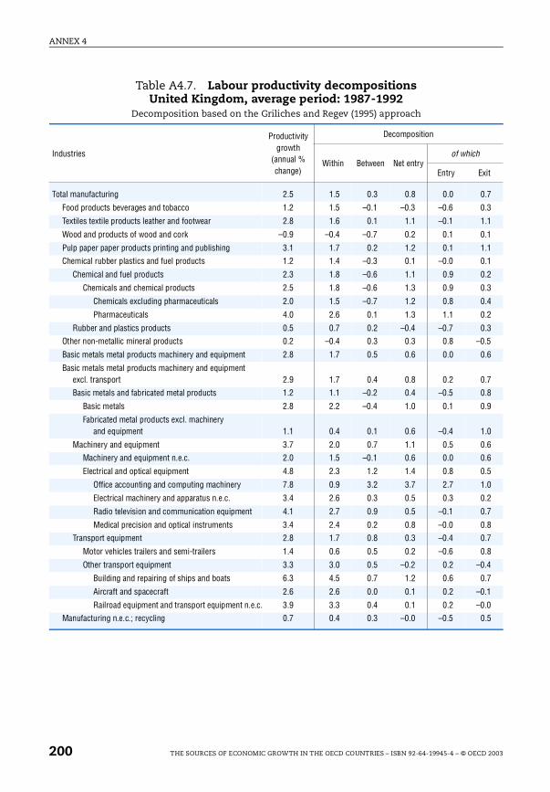
ANNEX 4
it
.7
.3
.1
.1
.1
.1
.2
.3
.4
.2
.3
.5
.6
.7
.8
.9
.0
.6
.6
.5
.0
.2
.7
.8
.7
.8
.4
.7
.1
.0
.5
Table A4.7. Labour productivity decompositions United Kingdom, average period: 1987-1992
Decomposition based on the Griliches and Regev (1995) approach
Industries
Productivity growth
(annual % change)
Decomposition
Within Between Net entryof which
Entry Ex
Total manufacturing 2.5 1.5 0.3 0.8 0.0 0
Food products beverages and tobacco 1.2 1.5 –0.1 –0.3 –0.6 0
Textiles textile products leather and footwear 2.8 1.6 0.1 1.1 –0.1 1
Wood and products of wood and cork –0.9 –0.4 –0.7 0.2 0.1 0
Pulp paper paper products printing and publishing 3.1 1.7 0.2 1.2 0.1 1
Chemical rubber plastics and fuel products 1.2 1.4 –0.3 0.1 –0.0 0
Chemical and fuel products 2.3 1.8 –0.6 1.1 0.9 0
Chemicals and chemical products 2.5 1.8 –0.6 1.3 0.9 0
Chemicals excluding pharmaceuticals 2.0 1.5 –0.7 1.2 0.8 0
Pharmaceuticals 4.0 2.6 0.1 1.3 1.1 0
Rubber and plastics products 0.5 0.7 0.2 –0.4 –0.7 0
Other non-metallic mineral products 0.2 –0.4 0.3 0.3 0.8 –0
Basic metals metal products machinery and equipment 2.8 1.7 0.5 0.6 0.0 0
Basic metals metal products machinery and equipment excl. transport 2.9 1.7 0.4 0.8 0.2 0
Basic metals and fabricated metal products 1.2 1.1 –0.2 0.4 –0.5 0
Basic metals 2.8 2.2 –0.4 1.0 0.1 0
Fabricated metal products excl. machinery and equipment 1.1 0.4 0.1 0.6 –0.4 1
Machinery and equipment 3.7 2.0 0.7 1.1 0.5 0
Machinery and equipment n.e.c. 2.0 1.5 –0.1 0.6 0.0 0
Electrical and optical equipment 4.8 2.3 1.2 1.4 0.8 0
Office accounting and computing machinery 7.8 0.9 3.2 3.7 2.7 1
Electrical machinery and apparatus n.e.c. 3.4 2.6 0.3 0.5 0.3 0
Radio television and communication equipment 4.1 2.7 0.9 0.5 –0.1 0
Medical precision and optical instruments 3.4 2.4 0.2 0.8 –0.0 0
Transport equipment 2.8 1.7 0.8 0.3 –0.4 0
Motor vehicles trailers and semi-trailers 1.4 0.6 0.5 0.2 –0.6 0
Other transport equipment 3.3 3.0 0.5 –0.2 0.2 –0
Building and repairing of ships and boats 6.3 4.5 0.7 1.2 0.6 0
Aircraft and spacecraft 2.6 2.6 0.0 0.1 0.2 –0
Railroad equipment and transport equipment n.e.c. 3.9 3.3 0.4 0.1 0.2 –0
Manufacturing n.e.c.; recycling 0.7 0.4 0.3 –0.0 –0.5 0
200 THE SOURCES OF ECONOMIC GROWTH IN THE OECD COUNTRIES – ISBN 92-64-19945-4 – © OECD 2003
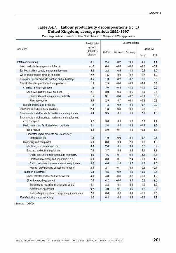
ANNEX 4
it
.1
.4
.0
.0
.9
.3
.2
.5
.6
.2
.2
.2
.6
.1
.5
.7
.5
.0
.9
.1
.8
.7
.0
.1
.4
.7
.6
.2
.7
.0
.3
Table A4.7. Labour productivity decompositions (cont.)United Kingdom, average period: 1992-1997
Decomposition based on the Griliches and Regev (1995) approach
Source: OECD.
Industries
Productivity growth
(annual % change)
Decomposition
Within Between Net entryof which
Entry Ex
Total manufacturing 3.1 2.4 –0.2 0.9 –0.1 1
Food products beverages and tobacco –1.0 0.4 –0.8 –0.6 –0.2 –0
Textiles textile products leather and footwear 2.8 2.2 –0.5 1.1 0.2 1
Wood and products of wood and cork 2.2 1.5 0.9 –0.2 –1.2 1
Pulp paper paper products printing and publishing 0.5 1.3 –0.2 –0.7 –1.6 0
Chemical rubber plastics and fuel products 1.3 2.5 –0.6 –0.6 –0.9 0
Chemical and fuel products 1.6 3.0 –0.4 –1.0 –1.1 0
Chemicals and chemical products 2.1 3.0 –0.4 –0.5 –1.0 0
Chemicals excluding pharmaceuticals 1.5 3.1 –0.8 –0.7 –1.3 0
Pharmaceuticals 3.4 2.9 0.7 –0.1 –0.3 0
Rubber and plastics products 1.2 1.8 –0.2 –0.4 –0.7 0
Other non-metallic mineral products 2.4 1.8 –0.3 0.9 0.7 0
Basic metals metal products machinery and equipment 5.4 3.5 0.1 1.8 0.2 1
Basic metals metal products machinery and equipment excl. transport 5.2 3.0 0.3 1.8 0.7 1
Basic metals and fabricated metal products 3.1 2.4 0.2 0.6 –0.9 1
Basic metals 4.4 3.0 –0.1 1.5 –0.2 1
Fabricated metal products excl. machinery and equipment 1.8 1.9 –0.0 –0.1 –0.7 0
Machinery and equipment 6.0 3.3 0.4 2.3 1.3 1
Machinery and equipment n.e.c. 3.8 2.8 0.1 0.9 0.0 0
Electrical and optical equipment 7.4 3.7 0.6 3.2 2.1 1
Office accounting and computing machinery 14.9 4.6 –0.1 10.4 5.6 4
Electrical machinery and apparatus n.e.c. 6.0 3.8 –0.1 2.4 0.7 1
Radio television and communication equipment 8.6 4.0 1.0 3.7 1.7 2
Medical precision and optical instruments 2.8 2.7 –0.1 0.1 0.2 –0
Transport equipment 6.3 4.5 –0.2 1.9 –0.5 2
Motor vehicles trailers and semi-trailers 4.9 4.8 –0.6 0.7 –1.0 1
Other transport equipment 7.6 4.2 –0.0 3.4 0.8 2
Building and repairing of ships and boats 4.1 3.8 0.1 0.2 –1.0 1
Aircraft and spacecraft 9.2 4.9 –0.1 4.5 1.8 2
Railroad equipment and transport equipment n.e.c. 2.0 0.6 0.6 0.9 –1.1 2
Manufacturing n.e.c.; recycling 2.0 0.8 0.3 0.9 –0.4 1
THE SOURCES OF ECONOMIC GROWTH IN THE OECD COUNTRIES – ISBN 92-64-19945-4 – © OECD 2003 201
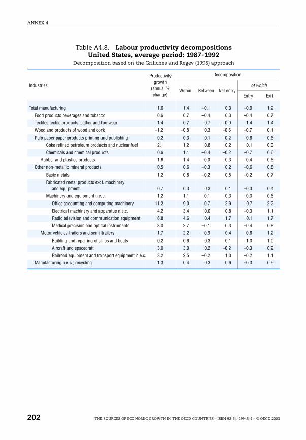
ANNEX 4
it
.2
.7
.4
.1
.6
.0
.6
.6
.8
.7
.4
.6
.2
.1
.7
.8
.2
.0
.2
.1
.9
Table A4.8. Labour productivity decompositionsUnited States, average period: 1987-1992
Decomposition based on the Griliches and Regev (1995) approach
Industries
Productivity growth
(annual % change)
Decomposition
Within Between Net entryof which
Entry Ex
Total manufacturing 1.6 1.4 –0.1 0.3 –0.9 1
Food products beverages and tobacco 0.6 0.7 –0.4 0.3 –0.4 0
Textiles textile products leather and footwear 1.4 0.7 0.7 –0.0 –1.4 1
Wood and products of wood and cork –1.2 –0.8 0.3 –0.6 –0.7 0
Pulp paper paper products printing and publishing 0.2 0.3 0.1 –0.2 –0.8 0
Coke refined petroleum products and nuclear fuel 2.1 1.2 0.8 0.2 0.1 0
Chemicals and chemical products 0.6 1.1 –0.4 –0.2 –0.7 0
Rubber and plastics products 1.6 1.4 –0.0 0.3 –0.4 0
Other non-metallic mineral products 0.5 0.6 –0.3 0.2 –0.6 0
Basic metals 1.2 0.8 –0.2 0.5 –0.2 0
Fabricated metal products excl. machinery and equipment 0.7 0.3 0.3 0.1 –0.3 0
Machinery and equipment n.e.c. 1.2 1.1 –0.1 0.3 –0.3 0
Office accounting and computing machinery 11.2 9.0 –0.7 2.9 0.7 2
Electrical machinery and apparatus n.e.c. 4.2 3.4 0.0 0.8 –0.3 1
Radio television and communication equipment 6.8 4.6 0.4 1.7 0.1 1
Medical precision and optical instruments 3.0 2.7 –0.1 0.3 –0.4 0
Motor vehicles trailers and semi-trailers 1.7 2.2 –0.9 0.4 –0.8 1
Building and repairing of ships and boats –0.2 –0.6 0.3 0.1 –1.0 1
Aircraft and spacecraft 3.0 3.0 0.2 –0.2 –0.3 0
Railroad equipment and transport equipment n.e.c. 3.2 2.5 –0.2 1.0 –0.2 1
Manufacturing n.e.c.; recycling 1.3 0.4 0.3 0.6 –0.3 0
202 THE SOURCES OF ECONOMIC GROWTH IN THE OECD COUNTRIES – ISBN 92-64-19945-4 – © OECD 2003
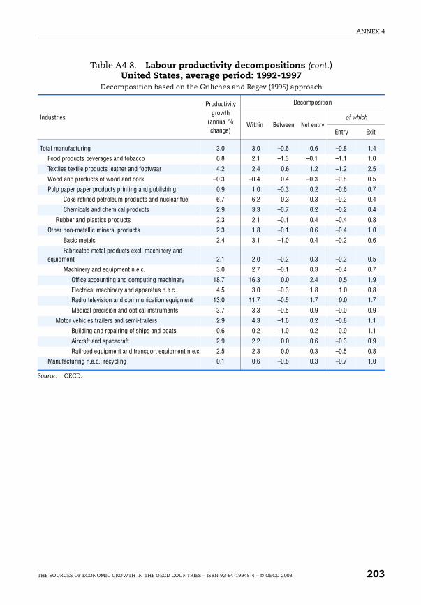
ANNEX 4
it
.4
.0
.5
.5
.7
.4
.4
.8
.0
.6
.5
.7
.9
.8
.7
.9
.1
.1
.9
.8
.0
Table A4.8. Labour productivity decompositions (cont.)United States, average period: 1992-1997
Decomposition based on the Griliches and Regev (1995) approach
Source: OECD.
Industries
Productivity growth
(annual % change)
Decomposition
Within Between Net entryof which
Entry Ex
Total manufacturing 3.0 3.0 –0.6 0.6 –0.8 1
Food products beverages and tobacco 0.8 2.1 –1.3 –0.1 –1.1 1
Textiles textile products leather and footwear 4.2 2.4 0.6 1.2 –1.2 2
Wood and products of wood and cork –0.3 –0.4 0.4 –0.3 –0.8 0
Pulp paper paper products printing and publishing 0.9 1.0 –0.3 0.2 –0.6 0
Coke refined petroleum products and nuclear fuel 6.7 6.2 0.3 0.3 –0.2 0
Chemicals and chemical products 2.9 3.3 –0.7 0.2 –0.2 0
Rubber and plastics products 2.3 2.1 –0.1 0.4 –0.4 0
Other non-metallic mineral products 2.3 1.8 –0.1 0.6 –0.4 1
Basic metals 2.4 3.1 –1.0 0.4 –0.2 0
Fabricated metal products excl. machinery and equipment 2.1 2.0 –0.2 0.3 –0.2 0
Machinery and equipment n.e.c. 3.0 2.7 –0.1 0.3 –0.4 0
Office accounting and computing machinery 18.7 16.3 0.0 2.4 0.5 1
Electrical machinery and apparatus n.e.c. 4.5 3.0 –0.3 1.8 1.0 0
Radio television and communication equipment 13.0 11.7 –0.5 1.7 0.0 1
Medical precision and optical instruments 3.7 3.3 –0.5 0.9 –0.0 0
Motor vehicles trailers and semi-trailers 2.9 4.3 –1.6 0.2 –0.8 1
Building and repairing of ships and boats –0.6 0.2 –1.0 0.2 –0.9 1
Aircraft and spacecraft 2.9 2.2 0.0 0.6 –0.3 0
Railroad equipment and transport equipment n.e.c. 2.5 2.3 0.0 0.3 –0.5 0
Manufacturing n.e.c.; recycling 0.1 0.6 –0.8 0.3 –0.7 1
THE SOURCES OF ECONOMIC GROWTH IN THE OECD COUNTRIES – ISBN 92-64-19945-4 – © OECD 2003 203
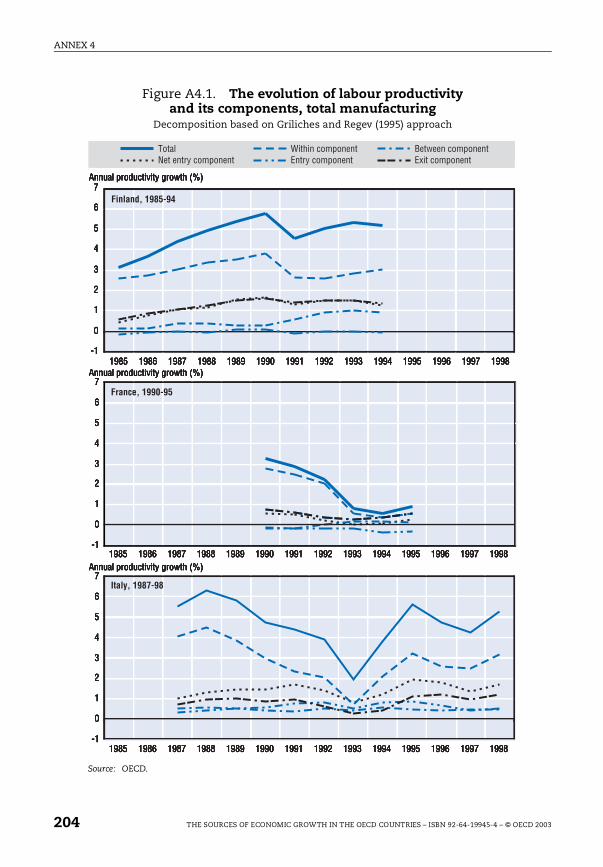
ANNEX 4
Figure A4.1. The evolution of labour productivity and its components, total manufacturing
Decomposition based on Griliches and Regev (1995) approach
Source: OECD.
-1
0
1
2
3
4
5
6
7
1985 1986 1987 1988 1989 1990 1991 1992 1993 1994 1995 1996 1997 1998
1985 1986 1987 1988 1989 1990 1991 1992 1993 1994 1995 1996 1997 1998
1985 1986 1987 1988 1989 1990 1991 1992 1993 1994 1995 1996 1997 1998
-1
0
1
2
3
4
5
6
7
-1
0
1
2
3
4
5
6
7
Total Within component Between component Net entry component Entry component Exit component
Finland, 1985-94
Annual productivity growth (%)
Annual productivity growth (%)
Annual productivity growth (%)
France, 1990-95
Italy, 1987-98
-1
0
1
2
3
4
5
6
7
1985 1986 1987 1988 1989 1990 1991 1992 1993 1994 1995 1996 1997 1998
1985 1986 1987 1988 1989 1990 1991 1992 1993 1994 1995 1996 1997 1998
1985 1986 1987 1988 1989 1990 1991 1992 1993 1994 1995 1996 1997 1998
-1
0
1
2
3
4
5
6
7
-1
0
1
2
3
4
5
6
7
Total Within component Between component Net entry component Entry component Exit component
Finland, 1985-94
Annual productivity growth (%)
Annual productivity growth (%)
Annual productivity growth (%)
France, 1990-95
Italy, 1987-98
204 THE SOURCES OF ECONOMIC GROWTH IN THE OECD COUNTRIES – ISBN 92-64-19945-4 – © OECD 2003
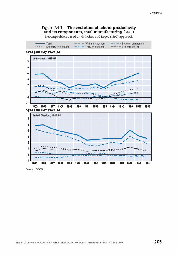
ANNEX 4
Figure A4.1. The evolution of labour productivity and its components, total manufacturing (cont.)Decomposition based on Griliches and Regev (1995) approach
Source: OECD.
-1
0
1
2
3
4
5
6
7
1985 1986 1987 1988 1989 1990 1991 1992 1993 1994 1995 1996 1997 1998
1985 1986 1987 1988 1989 1990 1991 1992 1993 1994 1995 1996 1997 1998-1
0
1
2
3
4
5
6
7
Total Within component Between component Net entry component Entry component Exit component
Netherlands, 1985-97
Annual productivity growth (%)
Annual productivity growth (%)
United Kingdom, 1985-98
THE SOURCES OF ECONOMIC GROWTH IN THE OECD COUNTRIES – ISBN 92-64-19945-4 – © OECD 2003 205
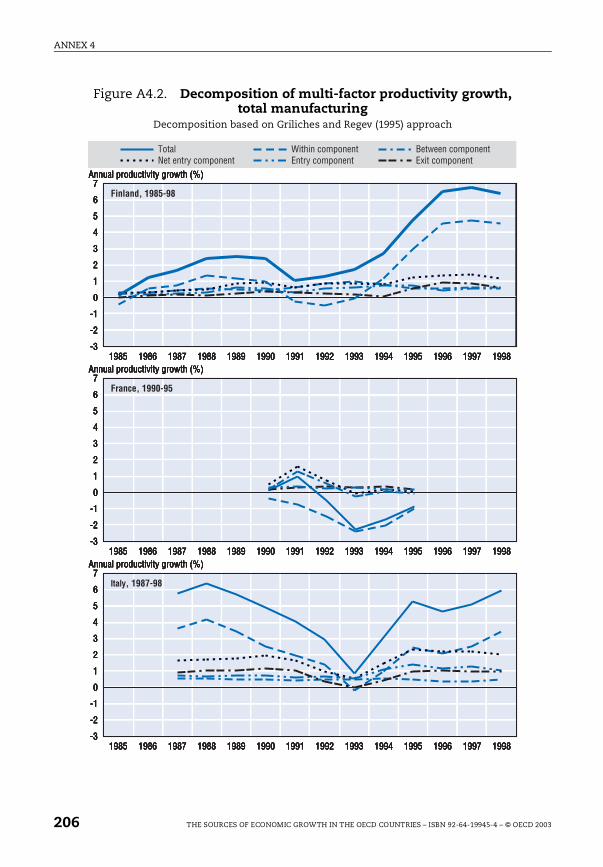
ANNEX 4
Figure A4.2. Decomposition of multi-factor productivity growth, total manufacturing
Decomposition based on Griliches and Regev (1995) approach
1985 1986 1987 1988 1989 1990 1991 1992 1993 1994 1995 1996 1997 1998
1985 1986 1987 1988 1989 1990 1991 1992 1993 1994 1995 1996 1997 1998
1985 1986 1987 1988 1989 1990 1991 1992 1993 1994 1995 1996 1997 1998
7
6
5
4
3
2
1
0
-1
-2
-3
7
6
5
4
3
2
1
0
-1
-2
-3
7
6
5
4
3
2
1
0
-1
-2
-3
Annual productivity growth (%)
Annual productivity growth (%)
Annual productivity growth (%)
Total Within component Between component Net entry component Entry component Exit component
Finland, 1985-98
Italy, 1987-98
France, 1990-95
1985 1986 1987 1988 1989 1990 1991 1992 1993 1994 1995 1996 1997 1998
1985 1986 1987 1988 1989 1990 1991 1992 1993 1994 1995 1996 1997 1998
1985 1986 1987 1988 1989 1990 1991 1992 1993 1994 1995 1996 1997 1998
7
6
5
4
3
2
1
0
-1
-2
-3
7
6
5
4
3
2
1
0
-1
-2
-3
7
6
5
4
3
2
1
0
-1
-2
-3
Annual productivity growth (%)
Annual productivity growth (%)
Annual productivity growth (%)
Total Within component Between component Net entry component Entry component Exit component
Finland, 1985-98
Italy, 1987-98
France, 1990-95
206 THE SOURCES OF ECONOMIC GROWTH IN THE OECD COUNTRIES – ISBN 92-64-19945-4 – © OECD 2003
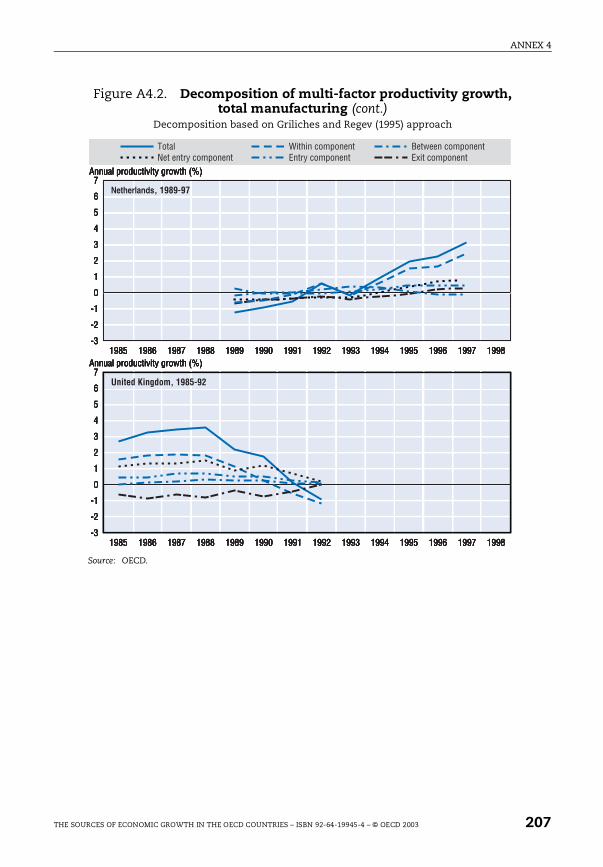
ANNEX 4
Figure A4.2. Decomposition of multi-factor productivity growth, total manufacturing (cont.)
Decomposition based on Griliches and Regev (1995) approach
Source: OECD.
1985 1986 1987 1988 1989 1990 1991 1992 1993 1994 1995 1996 1997 1998
1985 1986 1987 1988 1989 1990 1991 1992 1993 1994 1995 1996 1997 1998
7
6
5
4
3
2
1
0
-1
-2
-3
7
6
5
4
3
2
1
0
-1
-2
-3
Annual productivity growth (%)
Annual productivity growth (%)
Total Within component Between component Net entry component Entry component Exit component
Netherlands, 1989-97
United Kingdom, 1985-92
1985 1986 1987 1988 1989 1990 1991 1992 1993 1994 1995 1996 1997 1998
1985 1986 1987 1988 1989 1990 1991 1992 1993 1994 1995 1996 1997 1998
7
6
5
4
3
2
1
0
-1
-2
-3
7
6
5
4
3
2
1
0
-1
-2
-3
Annual productivity growth (%)
Annual productivity growth (%)
Total Within component Between component Net entry component Entry component Exit component
Netherlands, 1989-97
United Kingdom, 1985-92
THE SOURCES OF ECONOMIC GROWTH IN THE OECD COUNTRIES – ISBN 92-64-19945-4 – © OECD 2003 207
ANNEX 5
Annex 5
Basic data and sources
A5.1. Chapter 1
Data sources and links with national sources
The main source of data used in Chapter 1 is the OECD Economic Outlook
(EO) Database. Several specific adjustments were made to data on hours
worked, which are discussed below. Refined estimates of MFP growth alsorequired information drawn from additional sources. For example, data oncompositional changes of the capital stock and on the flow of capital servicesin nine countries were obtained from a recent OECD work (Colecchia andSchreyer, 2002). Similarly, the data needed to differentiate labour input by typeof worker were from OECD Education at a Glance, OECD Database (severalissues). Basic data for international comparison of income and productivitylevels are presented in Table A5.1.
In individual cases, a decision was taken to use alternative sources or toconstruct specific estimates in order to enhance time-series and cross-country comparability in the derived growth rates. Specific adjustments weremade for three countries: United Kingdom, Canada and United States. In aspecific subsection for each country, these adjustments are discussed andcompared with national sources. Among the most important adjustments arethose concerning capital stock series for the United States and Canada. Theseadjustments reflect efforts to use a gross capital stock measure forproductivity calculations, so as to be in line with the majority of data availablefor other countries.
Hours worked
Estimates of hours worked come mainly from national or EU sources:
For Austria, Belgium, Denmark, Greece, Ireland, Italy, Luxembourg,Netherlands, Portugal, and the United Kingdom, a country-specificadjustment has been applied to data from the European Labour ForceSurvey (EULFS). This adjustment factor varies by year and is obtained as theratio of adjusted versus non-adjusted estimates of hours worked based onthe EULFS under the assumption that there is a 50 per cent underestimation
208 THE SOURCES OF ECONOMIC GROWTH IN THE OECD COUNTRIES – ISBN 92-64-19945-4 – © OECD 2003
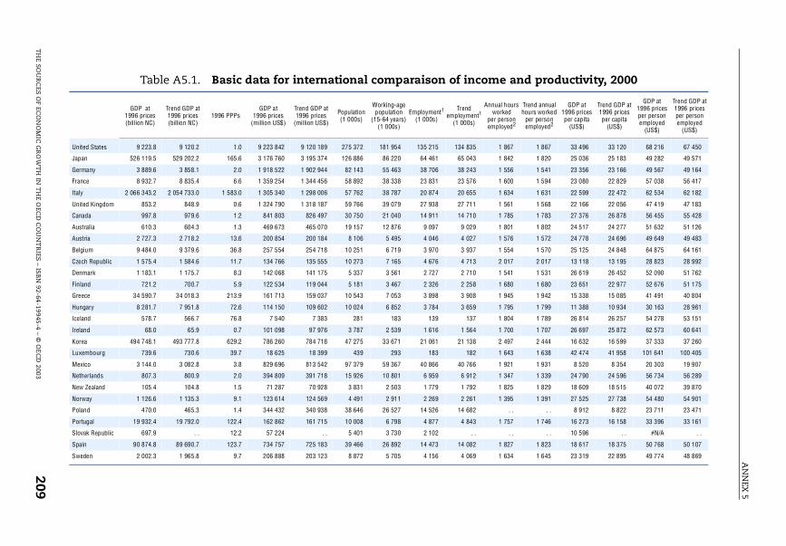
AN
NEX
5
TH
E SOU
RC
ES OF EC
ON
OM
IC G
RO
WT
H IN
TH
E OEC
D C
OU
NT
RIES
– ISB
N 92-64-19945-4 – ©
OE
CD
2003209
ome and productivity, 2000
Annual hours worked
per person employed2
Trend annual hours worked
per person employed2
GDP at 1996 prices per capita
(US$)
Trend GDP at 1996 prices per capita
(US$)
GDP at 1996 prices per person employed
(US$)
Trend GDP at 1996 prices per person employed
(US$)
1 867 1 867 33 496 33 120 68 216 67 450
1 842 1 820 25 036 25 183 49 282 49 571
1 556 1 541 23 356 23 166 49 567 49 164
1 600 1 594 23 080 22 829 57 038 56 417
1 634 1 631 22 599 22 472 62 534 62 182
1 561 1 568 22 166 22 056 47 419 47 183
1 785 1 783 27 376 26 878 56 455 55 428
1 801 1 802 24 517 24 277 51 632 51 126
1 576 1 572 24 778 24 696 49 649 49 483
1 554 1 570 25 125 24 848 64 875 64 161
2 017 2 017 13 118 13 195 28 823 28 992
1 541 1 531 26 619 26 452 52 090 51 762
1 680 1 680 23 651 22 977 52 676 51 175
1 945 1 942 15 338 15 085 41 491 40 804
1 795 1 799 11 388 10 934 30 163 28 961
1 804 1 789 26 814 26 257 54 278 53 151
1 700 1 707 26 697 25 872 62 573 60 641
2 497 2 444 16 632 16 599 37 333 37 260
1 643 1 638 42 474 41 958 101 641 100 405
1 921 1 931 8 520 8 354 20 303 19 907
1 347 1 339 24 790 24 596 56 734 56 289
1 825 1 829 18 609 18 515 40 072 39 870
1 395 1 391 27 525 27 738 54 480 54 901
. . . . 8 912 8 822 23 711 23 471
1 757 1 746 16 273 16 158 33 396 33 161
. . . . 10 596 . . #N/A . .
1 827 1 823 18 617 18 375 50 768 50 107
1 634 1 645 23 319 22 895 49 774 48 869
Table A5.1. Basic data for international comparaison of inc
GDP at 1996 prices (billion NC)
Trend GDP at1996 prices(billion NC)
1996 PPPsGDP at
1996 prices (million US$)
Trend GDP at 1996 prices
(million US$)
Population (1 000s)
Working-age population
(15-64 years) (1 000s)
Employment1 (1 000s)
Trend employment1
(1 000s)
United States 9 223.8 9 120.2 1.0 9 223 842 9 120 189 275 372 181 954 135 215 134 835
Japan 526 119.5 529 202.2 165.6 3 176 760 3 195 374 126 886 86 220 64 461 65 043
Germany 3 889.6 3 858.1 2.0 1 918 522 1 902 944 82 143 55 463 38 706 38 243
France 8 932.7 8 835.4 6.6 1 359 254 1 344 456 58 892 38 338 23 831 23 576
Italy 2 066 343.2 2 054 733.0 1 583.0 1 305 340 1 298 006 57 762 38 787 20 874 20 655
United Kingdom 853.2 848.9 0.6 1 324 790 1 318 187 59 766 39 079 27 938 27 711
Canada 997.8 979.6 1.2 841 803 826 497 30 750 21 040 14 911 14 710
Australia 610.3 604.3 1.3 469 673 465 070 19 157 12 876 9 097 9 029
Austria 2 727.3 2 718.2 13.6 200 854 200 184 8 106 5 495 4 046 4 027
Belgium 9 484.0 9 379.6 36.8 257 554 254 718 10 251 6 719 3 970 3 937
Czech Republic 1 575.4 1 584.6 11.7 134 766 135 555 10 273 7 165 4 676 4 713
Denmark 1 183.1 1 175.7 8.3 142 068 141 175 5 337 3 561 2 727 2 710
Finland 721.2 700.7 5.9 122 534 119 044 5 181 3 467 2 326 2 258
Greece 34 590.7 34 018.3 213.9 161 713 159 037 10 543 7 053 3 898 3 908
Hungary 8 281.7 7 951.8 72.6 114 150 109 602 10 024 6 852 3 784 3 659
Iceland 578.7 566.7 76.8 7 540 7 383 281 183 139 137
Ireland 68.0 65.9 0.7 101 098 97 976 3 787 2 539 1 616 1 564
Korea 494 748.1 493 777.8 629.2 786 260 784 718 47 275 33 671 21 061 21 138
Luxembourg 739.6 730.6 39.7 18 625 18 399 439 293 183 182
Mexico 3 144.0 3 082.8 3.8 829 696 813 542 97 379 59 367 40 866 40 766
Netherlands 807.3 800.9 2.0 394 809 391 718 15 926 10 801 6 959 6 912
New Zealand 105.4 104.8 1.5 71 287 70 928 3 831 2 503 1 779 1 792
Norway 1 126.6 1 135.3 9.1 123 614 124 569 4 491 2 911 2 269 2 261
Poland 470.0 465.3 1.4 344 432 340 938 38 646 26 527 14 526 14 682
Portugal 19 932.4 19 792.0 122.4 162 862 161 715 10 008 6 798 4 877 4 843
Slovak Republic 697.9 . . 12.2 57 224 . . 5 401 3 730 2 102 . .
Spain 90 874.8 89 690.7 123.7 734 757 725 183 39 466 26 892 14 473 14 082
Sweden 2 002.3 1 965.8 9.7 206 888 203 123 8 872 5 705 4 156 4 069
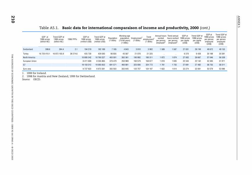
AN
NEX
5
210T
HE S
OU
RC
ES O
F EC
ON
OM
IC G
RO
WT
H IN
TH
E OEC
D C
OU
NT
RIES – ISB
N 92-64-19945-4 – ©
OEC
D 2003
e and productivity, 2000 (cont.)
Annual hours worked
per person employed2
Trend annual hours worked
per person employed2
GDP at 1996 prices per capita
(US$)
Trend GDP at 1996 prices per capita
(US$)
GDP at 1996 prices per person employed
(US$)
Trend GDP at 1996 prices per person employed
(US$)
1 589 1 587 27 031 26 749 49 672 49 153
. . . . 6 370 6 428 20 198 20 381
1 872 1 874 27 002 26 667 57 046 56 339
1 610 1 605 22 343 22 142 52 383 51 911
1 761 1 755 27 691 27 482 58 755 58 311
1 622 1 614 22 274 22 061 53 579 53 066
Table A5.1. Basic data for international comparaison of incom
1. 1999 for Ireland.2. 1998 for Austria and New Zealand, 1999 for Switzerland.Source: OECD.
GDP at 1996 prices (billion NC)
Trend GDP at1996 prices(billion NC)
1996 PPPsGDP at
1996 prices (million US$)
Trend GDP at 1996 prices
(million US$)
Population (1 000s)
Working-age population
(15-64 years) (1 000s)
Employment1 (1 000s)
Trend employment1
(1 000s)
Switzerland 398.6 394.4 2.1 194 219 192 189 7 185 4 843 3 910 3 902
Turkey 16 720 410.1 16 872 105.9 39 274.6 425 730 429 593 66 835 43 587 21 078 21 325
North America 10 895 342 10 760 227 403 501 262 361 190 992 190 311
European Union 8 411 669 8 335 865 376 479 250 989 160 579 158 677
G7 19 150 312 19 005 653 691 571 460 881 325 936 324 772
Euro area 6 737 923 6 673 381 302 503 202 645 125 757 124 187
ANNEX 5
of time lost due to illness and maternity. The average adjustment factor for
the countries reported above is 0.97.
For Finland and Iceland, an average adjustment factor derived from theEULFS has been applied to national Labour Force Survey (LFS) estimates dueto the limited length of EULFS series.
For Australia, Czech Republic, Korea, and New Zealand, data come fromnational LFS, adjusted with the average adjustment factor of 0.97.
For Canada, France, Germany, Hungary, Japan, Norway, Spain, Sweden, andSwitzerland, data are national estimates (either from LFS, or from nationalaccounts/enterprise surveys). For the United States data are the BLSestimate of total hours worked on the basis of the Current PopulationSurvey, the Current Employment Statistics, and the Hours at Work Survey,divided by the average number of employed persons.
For Mexico hours worked are based on a level estimate from Maddison(1995) for 1992 and a time series from the National Survey of Employment(see OECD, 1999c, for more detailed information on national sources).
Where possible, estimates have also been extended backwards throughsplicing with the estimates from Maddison (1995). See Scarpetta et al. (2000)for more details.
United States
Output
Small differences occur, because the OECD Economic Outlook (EO)business sector data is based on national income and product accounts data.Also, the BLS business sector output measures exclude governmententerprises to be fully consistent with its capital input series. The OECD seriesdoes not make this adjustment and therefore includes governmententerprises. Also, the adjustment in the EO database to move from anaggregate for the total economy to the value-added of the business sector is
not identical to national procedures.
Labour
The number of persons in the OECD series is taken from employmentdata as published in the United States’ National Income and ProductAccounts. It reflects persons employed in production, i.e. the number ofemployees plus self-employed. Hours worked per person were derived
separately, as discussed above. BLS, in its multi-factor productivity series, usesan index of labour input. Conceptually, the measure of labour input is similarto the OECD’s labour input measure as described in Annex 1: it reflects totalhours worked, adjusted for changes in the composition of the quality of
THE SOURCES OF ECONOMIC GROWTH IN THE OECD COUNTRIES – ISBN 92-64-19945-4 – © OECD 2003 211
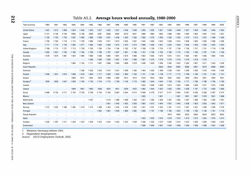
AN
NEX
5
212T
HE S
OU
RC
ES O
F EC
ON
OM
IC G
RO
WT
H IN
TH
E OEC
D C
OU
NT
RIES – ISB
N 92-64-19945-4 – ©
OEC
D 2003
Table A5.2. Average hours worked annually, 1980-2000
1993 1994 1995 1996 1997 1998 1999 2000
1 837 1 839 1 848 1 837 1 849 1 850 1 846 1 835
1905 1 898 1 884 1 892 1 864 1 842 1 810 1 821
1 556 1 555 1 535 1 519 1 513 1 507 1 496 1 482
1 642 1 639 1 614 1 608 1 605 1 603 1 596 1 590
1 637 1 634 1 635 1 636 1 640 1 629 1 625 1 622
1 723 1 737 1 739 1 738 1 737 1 731 1 719 1 708
1 763 1 780 1 775 1 784 1 790 1 787 1 791 1 795
1 870 1 875 1 872 1 862 1 861 1 856 1 860 1 855
1 576 1 576 1 576 1 576 1 576 1 576 . . . .
1 590 1 592 1 622 1 594 1 607 1 611 1 553 1 530
. 2064 2043 2064 2066 2067 2075 2088 2092
1 469 1 539 1 501 1 509 1 520 1 519 1 544 1 504
1 739 1 777 1 772 1 789 1 780 1 761 1 765 1 721
1964 1932 1922 1939 1924 1921 1940 1921
1 644 1 759 1 765 1 777 1 786 1 788 1 795 1 795
1 828 1 813 1 832 1 860 1 839 1 817 1 873 1 885
1 832 1 835 1 835 1 836 1 797 1 722 1 693 1 690
2 477 2 471 2 484 2 467 2 436 2 390 2 497 2 474
. 1 821 . . 1 857 1901 1927 1 878 1921 1 888
1 364 1 391 1 365 1 387 1 380 1 364 1 345 1 381
1 844 1 851 1 843 1 838 1 823 1 825 1 842 1 817
1 434 1 431 1 414 1 407 1 401 1 400 1 395 1 376
1 788 1 784 1 822 1 799 1 760 1 746 1 761 1 719
. . . 1975 1993 2023 2055 2034 2022 2023
1 816 1 816 1 815 1 810 1 813 1 834 1 816 1 814
1 570 1 602 1 614 1 623 1 628 1 629 1 636 1 625
1 607 1 623 1 599 1 595 1 589 1 589 1 597 1 568
1. Western Germany before 1991.2. Dependent employment.Source: OECD Employment Outlook, 2002.
Total economy 1980 1981 1982 1983 1984 1985 1986 1987 1988 1989 1990 1991 1992
United States 1 822 1 812 1 806 1 824 1 840 1 835 1 827 1 833 1 837 1 848 1 838 1 826 1 828
Japan 2 121 2 106 2 104 2095 2 108 2093 2097 2096 2092 2070 2031 1998 1965
Germany1 1 720 1 703 1 703 1 697 1 690 1 666 1 659 1 647 1 646 1 620 1 583 1 560 1 576
France 1 795 1 760 1 718 1 712 1 700 1 685 1 676 1 671 1 673 1 655 1 657 1 645 1 646
Italy 1 717 1 710 1 703 1 692 1 677 1 665 1 663 1 658 1 675 1 672 1 674 1 668 1 636
United Kingdom 1 769 1 712 1 727 1 713 1 729 1 762 1 765 1 754 1 794 1 782 1 767 1 768 1 729
Canada 1 802 1 801 1 784 1 780 1 782 1 790 1 789 1 797 1 807 1 801 1 788 1 767 1 759
Australia 1 878 1 878 1 867 1 853 1 869 1 866 1 848 1 860 1 881 1 870 1 866 1 853 1 845
Austria . . . . . . . . . . 1 595 1 595 1 595 1 607 1 591 1 586 1 581 1 576
Belgium . . . . . . 1 684 1 704 1 711 1 697 1 686 1 680 1 668 1 679 1 646 1 629
Czech Republic . . . . . . . . . . . . . . . . . . . . . . . . .
Denmark . . . . . . . . 1 536 1 553 1 534 1 514 1 531 1 508 1 492 1 484 1 503
Finland 1 846 1 831 1 810 1 809 1 810 1 804 1 777 1 802 1 824 1 802 1 763 1 741 1 762
Greece . . . . . . 1983 1917 1945 1929 1 889 1 882 1913 1912 1916 1944
Hungary2 1930 1928 1 847 1 829 1 765 1 742 1 734 1 772 1 768 1 746 1 710 1 682 1 644
Iceland . . . . . . . . . . . . . . . . . . . . . . 1 843 1 859
Ireland . . . . . . 1909 1901 1905 1936 1924 1921 1929 1922 1 892 1 844
Korea 2 689 2 705 2 717 2 734 2 730 2 706 2 734 2 705 2 662 2 564 2 514 2 498 2 478
Mexico . . . . . . . . . . . . . . . . . . . . . . 1 822 .
Netherlands . . . . . . . . . . 1 437 . . 1 514 1 480 1 469 1 454 1 427 1 393
New Zealand . . . . . . . . . . . . . . 1 851 1 845 1 832 1 820 1 802 1 812
Norway 1 512 1 502 1 490 1 485 1 479 1 473 1 469 1 443 1 444 1 440 1 432 1 427 1 437
Portugal . . . . . . . . . . . . 1 842 1 861 1 859 1 889 1 882 1 808 1 797
Slovak Republic . . . . . . . . . . . . . . . . . . . . . . . . .
Spain . . . . . . . . . . . . . . . . . . . . . . 1 833 1 825
Sweden 1 505 1 497 1 511 1 520 1 522 1 526 1 524 1 534 1 553 1 552 1 549 1 536 1 553
Switzerland . . . . . . . . . . . . . . . . . . . . . . 1 606 1 605
ANNEX 5
labour. Although BLS is able to use a much finer level of differentiation
between types of labour, the two labour input measures differ only slightlyover the period under consideration. While this difference would appearsmall, it may be the result of compensating differences or simply due to thespecific period chosen for comparison.
Capital
As pointed out earlier, for its basic MFP series, OECD uses an estimated
measure of the gross capital stock,1 while available data in the EO databaserefer to a concept of net capital stock as published by BEA. BLS, akin to itslabour input measure, uses a measure of capital services that reflects both thequantity and the changing composition of capital input. The underlyingconcept is briefly described in Annex 1 as well as in Chapter 1. As expected,the gross capital stock measure grows by much less than BLS’ capital servicemeasure. However, there is significant similarity between OECD’s capitalservice series and that of BLS. The construction of the OECD capital servicedata is described above.
Canada
Output
There are only minor differences between OECD business sector seriesand the ones published by Statistics Canada, due to differences in thedefinition of the business sector.
Labour
The number of persons in the OECD series is taken from employmentdata as published by Statistics Canada’s Input-Output Division. Series on boththe number of persons and on total hours are available. Statistics Canada, inits multi-factor productivity series, uses an index of labour input.Conceptually, this labour input measure is not as elaborate as the one used byBLS but is more developed than a simple sum of all hours worked.Differentiation takes place by industry, because each industry’s contributionto the economy’s labour input is weighted by the share that a given industryoccupies in the economy’s total labour compensation. If average wages in anindustry exceed those of other sectors, an implicit weighting of hours byindustry takes place. However, there is no explicit differentiation byeducational attainment or the skills of workers.
Capital
As pointed out earlier, for its basic MFP series, OECD uses an estimatedmeasure of the gross capital stock. For Canada, gross capital stock is the
THE SOURCES OF ECONOMIC GROWTH IN THE OECD COUNTRIES – ISBN 92-64-19945-4 – © OECD 2003 213
ANNEX 5
Statistics Canada capital stock series that is constructed on a one-hoss shay
age-efficiency pattern. Statistics Canada’s own MFP calculations use as inputanother of their capital stock series, one based on a geometric age-efficiencypattern. A second difference lies in the aggregation procedure: StatisticsCanada uses a Fisher index number formula to aggregate capital input acrossindustries. The gross capital stock measure used by OECD is based on aLaspeyres-type aggregation formula. Again, the final outcome does not differby much, although this reflects the combined, and partly offsetting, effects ofa different age-efficiency pattern and a different index number formula.
United Kingdom
In the United Kingdom, time series for business sector GDP andemployment have been corrected to take into account the fact that theNational Health Service (NHS) Trust, created in 1991, is not accounted for inthe government sector. Conversely all public health services were accountedfor in the government sector before 1991. For comparability reasons bothemployment and GDP of NHS Trust have been subtracted from business sectorseries. The method of calculation of GDP of NHS Trust is as follows: first on thebasis of United Kingdom Abstract of Statistics, 1998, a productivity level at
current prices of NHS Staff was computed on the basis of Total CurrentExpenditure on the NHS (item KJQJ) and Total Employment of NHS (itemsKDBC+KDBO+KWUH). Then a real (at 1995 prices) productivity was computedthrough the implicit deflator of Health and Social Work sector (Sector N in theNational Accounts – National Accounts, 1998 – Blue Book). Then thisproductivity was applied to data on NHS Trust staff.
A5.2. Chapter 2
The data used in Chapter 2 are from the following sources:
Data on GDP, working age population, gross fixed capital formation, generalgovernment current nominal tax and non-tax receipts, direct and indirecttaxes, government nominal final consumption and imports and exports are
from the OECD Economic Outlook (EO) Data Base. Purchasing Power Paritybenchmarks for 1993 are from the OECD Statistics Directorate. In the case ofNorway, data refer to the mainland economy. In the case of Greece andPortugal the ratio between total gross fixed capital formation and total realGDP was used as a proxy for the investment rate (i.e. the ratio of privatenon-residential fixed capital formation to business sector real GDP), due todata availability.
Data on Research and Development (R&D) are from the OECD Main Scienceand Technology Indicators (MSTI) database. A few missing observationswere obtained by interpolation.
214 THE SOURCES OF ECONOMIC GROWTH IN THE OECD COUNTRIES – ISBN 92-64-19945-4 – © OECD 2003
ANNEX 5
Data on human capital are calculated on the basis of raw data on
educational attainment from De la Fuente and Doménech (2000)2 and fromthe OECD Education at a Glance (various issues). In particular: threeeducational groups were considered: below upper secondary education(ISCED 0 to ISCED 2); upper secondary education (ISCED 3); and tertiaryeducation (ISCED 5 to ISCED 7). For the 1990s, the level of educationalattainment for male and female workers is available from matched OECDsources for the following countries: Australia, Canada, Denmark, Finland,France, Germany, Ireland, Italy, the Netherlands, New Zealand, Norway,Portugal, Sweden, United Kingdom, United States. For Austria, Belgium,Czech Republic, Greece, Hungary, Korea, Mexico, Poland, Spain, Switzerlandand Turkey the calculation of labour input was not possible due to theunavailability of either the educational composition of employment or
relative wages by education level. Until the early 1980s, data on educationalattainment are interpolated from five-year observations from De la Fuenteand Doménech (2000). The cumulative years of schooling by educationallevel – required to estimate the average number of years of total schoolingused in the empirical analysis – are from the OECD Education at a Glance 1997(OECD, 1998c).
The indicators measuring financial market developments are discussedin Leahy et al. (2001).
The definition of each variable is provided in Box 2.3 of Chapter 2. Theexact country coverage of the variables, as well as basic statistics, can befound in Annex 1 of Bassanini et al. (2001).
A5.3. Chapter 3
Industry-level data
Productivity data
The industry-level data used in section 3.1 of Chapter 3 comes fromdifferent versions of the structural analysis (STAN) database. The industriesconsidered in the productivity analysis of Chapters 3 and 4 – and, formanufacturing, their classification according to the market structuretypologies discussed in Box 3.4 of Chapter 3 – are presented in Table A5.4,while Table A5.5 presents the coverage of the available data. Three main data-sets have been used to construct the value-added, capital stock, employmentand labour compensation series necessary to compute multifactorproductivity series at the firm-level. The main data-set is the OECD STAN-2000 database. It was updated for missing series from other OECD database
(e.g. ISDB, STAN-1998, and STAN-1992) for a small subset of sectors3 for whichdisaggregated data were not available in the other data-sets.
THE SOURCES OF ECONOMIC GROWTH IN THE OECD COUNTRIES – ISBN 92-64-19945-4 – © OECD 2003 215
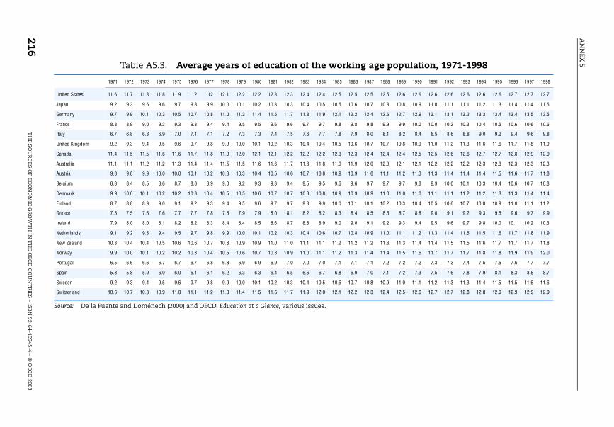
AN
NEX
5
216T
HE S
OU
RC
ES O
F EC
ON
OM
IC G
RO
WT
H IN
TH
E OEC
D C
OU
NT
RIES – ISB
N 92-64-19945-4 – ©
OEC
D 2003
e population, 1971-1998
1988 1989 1990 1991 1992 1993 1994 1995 1996 1997 1998
12.5 12.6 12.6 12.6 12.6 12.6 12.6 12.6 12.7 12.7 12.7
10.8 10.8 10.9 11.0 11.1 11.1 11.2 11.3 11.4 11.4 11.5
12.6 12.7 12.9 13.1 13.1 13.2 13.3 13.4 13.4 13.5 13.5
9.9 9.9 10.0 10.0 10.2 10.3 10.4 10.5 10.6 10.6 10.6
8.1 8.2 8.4 8.5 8.6 8.8 9.0 9.2 9.4 9.6 9.8
10.7 10.8 10.9 11.0 11.2 11.3 11.6 11.6 11.7 11.8 11.9
12.4 12.4 12.5 12.5 12.6 12.6 12.7 12.7 12.8 12.9 12.9
12.0 12.1 12.1 12.2 12.2 12.2 12.3 12.3 12.3 12.3 12.3
11.1 11.2 11.3 11.3 11.4 11.4 11.4 11.5 11.6 11.7 11.8
9.7 9.7 9.8 9.9 10.0 10.1 10.3 10.4 10.6 10.7 10.8
11.0 11.0 11.0 11.1 11.1 11.2 11.2 11.3 11.3 11.4 11.4
10.2 10.3 10.4 10.5 10.6 10.7 10.8 10.9 11.0 11.1 11.2
8.6 8.7 8.8 9.0 9.1 9.2 9.3 9.5 9.6 9.7 9.9
9.2 9.3 9.4 9.5 9.6 9.7 9.8 10.0 10.1 10.2 10.3
11.0 11.1 11.2 11.3 11.4 11.5 11.5 11.6 11.7 11.8 11.9
11.3 11.3 11.4 11.4 11.5 11.5 11.6 11.7 11.7 11.7 11.8
11.4 11.5 11.6 11.7 11.7 11.7 11.8 11.8 11.9 11.9 12.0
7.2 7.2 7.2 7.3 7.3 7.4 7.5 7.5 7.6 7.7 7.7
7.1 7.2 7.3 7.5 7.6 7.8 7.9 8.1 8.3 8.5 8.7
10.9 11.0 11.1 11.2 11.3 11.3 11.4 11.5 11.5 11.6 11.6
12.4 12.5 12.6 12.7 12.7 12.8 12.8 12.9 12.9 12.9 12.9
Table A5.3. Average years of education of the working ag
Source: De la Fuente and Doménech (2000) and OECD, Education at a Glance, various issues.
1971 1972 1973 1974 1975 1976 1977 1978 1979 1980 1981 1982 1983 1984 1985 1986 1987
United States 11.6 11.7 11.8 11.8 11.9 12 12 12.1 12.2 12.2 12.3 12.3 12.4 12.4 12.5 12.5 12.5
Japan 9.2 9.3 9.5 9.6 9.7 9.8 9.9 10.0 10.1 10.2 10.3 10.3 10.4 10.5 10.5 10.6 10.7
Germany 9.7 9.9 10.1 10.3 10.5 10.7 10.8 11.0 11.2 11.4 11.5 11.7 11.8 11.9 12.1 12.2 12.4
France 8.8 8.9 9.0 9.2 9.3 9.3 9.4 9.4 9.5 9.5 9.6 9.6 9.7 9.7 9.8 9.8 9.8
Italy 6.7 6.8 6.8 6.9 7.0 7.1 7.1 7.2 7.3 7.3 7.4 7.5 7.6 7.7 7.8 7.9 8.0
United Kingdom 9.2 9.3 9.4 9.5 9.6 9.7 9.8 9.9 10.0 10.1 10.2 10.3 10.4 10.4 10.5 10.6 10.7
Canada 11.4 11.5 11.5 11.6 11.6 11.7 11.8 11.9 12.0 12.1 12.1 12.2 12.2 12.2 12.3 12.3 12.4
Australia 11.1 11.1 11.2 11.2 11.3 11.4 11.4 11.5 11.5 11.6 11.6 11.7 11.8 11.8 11.9 11.9 12.0
Austria 9.8 9.8 9.9 10.0 10.0 10.1 10.2 10.3 10.3 10.4 10.5 10.6 10.7 10.8 10.9 10.9 11.0
Belgium 8.3 8.4 8.5 8.6 8.7 8.8 8.9 9.0 9.2 9.3 9.3 9.4 9.5 9.5 9.6 9.6 9.7
Denmark 9.9 10.0 10.1 10.2 10.2 10.3 10.4 10.5 10.5 10.6 10.7 10.7 10.8 10.8 10.9 10.9 10.9
Finland 8.7 8.8 8.9 9.0 9.1 9.2 9.3 9.4 9.5 9.6 9.7 9.7 9.8 9.9 10.0 10.1 10.1
Greece 7.5 7.5 7.6 7.6 7.7 7.7 7.8 7.8 7.9 7.9 8.0 8.1 8.2 8.2 8.3 8.4 8.5
Ireland 7.9 8.0 8.0 8.1 8.2 8.2 8.3 8.4 8.4 8.5 8.6 8.7 8.8 8.9 9.0 9.0 9.1
Netherlands 9.1 9.2 9.3 9.4 9.5 9.7 9.8 9.9 10.0 10.1 10.2 10.3 10.4 10.6 10.7 10.8 10.9
New Zealand 10.3 10.4 10.4 10.5 10.6 10.6 10.7 10.8 10.9 10.9 11.0 11.0 11.1 11.1 11.2 11.2 11.2
Norway 9.9 10.0 10.1 10.2 10.2 10.3 10.4 10.5 10.6 10.7 10.8 10.9 11.0 11.1 11.2 11.3 11.4
Portugal 6.5 6.6 6.6 6.7 6.7 6.7 6.8 6.8 6.9 6.9 6.9 7.0 7.0 7.0 7.1 7.1 7.1
Spain 5.8 5.8 5.9 6.0 6.0 6.1 6.1 6.2 6.3 6.3 6.4 6.5 6.6 6.7 6.8 6.9 7.0
Sweden 9.2 9.3 9.4 9.5 9.6 9.7 9.8 9.9 10.0 10.1 10.2 10.3 10.4 10.5 10.6 10.7 10.8
Switzerland 10.6 10.7 10.8 10.9 11.0 11.1 11.2 11.3 11.4 11.5 11.6 11.7 11.9 12.0 12.1 12.2 12.3
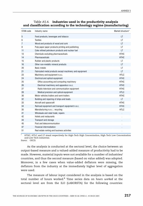
ANNEX 5
g)
ation
ure*
As the analysis is conducted at the sectoral level, the choice between anoutput-based measure and a valued-added measure of productivity had to bemade. However, material inputs were not available for a number of industries/countries, and thus the second measure (based on value added) was adopted.Moreover, in a few cases when value-added deflators were missing, thedeflators from the industry at the immediately higher level of aggregationwere used.
The measure of labour input considered in the analysis is based on thetotal number of hours worked.4 Time series data on hours worked at thesectoral level are from the ILO (LABORSTA) for the following countries:
Table A5.4. Industries used in the productivity analysis and classification according to the technology regime (manufacturin
* HTHC, HTLC and LT stand respectively for High-Tech High Concentration, High-Tech Low Concentrand Low-Tech industries.
Source: OECD.
STAN code Industry name Market struct
5 Food products, beverages and tobacco LT
6 Textiles LT
7 Wood and products of wood and cork LT
8 Pulp paper paper products printing and publishing LT
11 Coke refined petroleum products and nuclear fuel LT
13 Chemicals excluding pharmaceuticals HTHC
14 Pharmaceuticals HTHC
15 Rubber and plastic products LT
16 Other non-metallic mineral products LT
20 Basic metals LT
21 Fabricated metal products except machinery and equipment LT
23 Machinery and equipment n.e.c. HTLC
24 Electrical and optical equipment HTHC
25 Office accounting and computing machinery HTHC
26 Electrical machinery and apparatus n.e.c. HTHC
27 Radio television and communication equipment HTHC
28 Medical precision and optical equipment HTLC
30 Motor vehicles trailers and semi-trailers HTHC
32 Building and repairing of ships and boats LT
33 Aircraft and spacecraft HTHC
34 Railroad equipment and transport equipment n.e.c. HTHC
35 Manufacturing n.e.c. ; recycling HTLC
41 Wholesale and retail trade; repairs .
42 Hotels and restaurants .
44 Transport and storage .
45 Post and telecommunication .
47 Financial intermediation .
51 Real estate renting and business activities .
THE SOURCES OF ECONOMIC GROWTH IN THE OECD COUNTRIES – ISBN 92-64-19945-4 – © OECD 2003 217
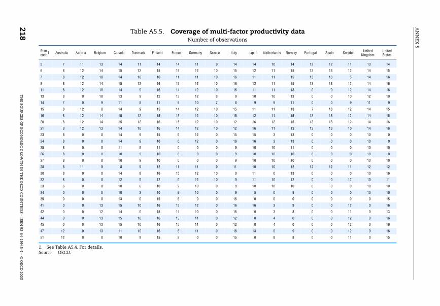
AN
NEX
5
218T
HE S
OU
RC
ES O
F EC
ON
OM
IC G
RO
WT
H IN
TH
E OEC
D C
OU
NT
RIES – ISB
N 92-64-19945-4 – ©
OEC
D 2003
Table A5.5. Coverage of multi-factor productivity data
erlands Norway Portugal Spain Sweden United Kingdom
UnitedStates
10 14 12 12 11 13 14
11 15 13 13 12 14 15
11 15 13 13 5 14 16
11 15 13 13 12 14 16
11 13 0 9 12 14 16
10 13 0 0 10 12 10
9 11 0 0 9 11 9
11 13 7 13 12 14 15
11 15 13 13 12 14 15
12 15 13 13 12 14 16
11 13 13 13 10 14 16
3 13 0 0 0 10 0
3 13 0 0 0 10 0
10 11 0 0 0 10 10
10 10 0 0 0 10 0
10 10 0 0 0 10 10
10 12 12 12 11 12 12
0 13 0 0 0 10 16
10 12 0 0 12 10 11
10 10 0 0 0 10 10
0 9 0 0 0 10 10
0 0 0 0 0 0 15
3 9 0 0 12 0 16
3 8 0 0 11 0 13
4 0 0 0 12 0 16
4 0 0 0 12 0 16
0 9 0 0 12 0 16
8 8 0 0 11 0 15
Number of observations
1. See Table A5.4. For details.Source: OECD.
Stan code1 Australia Austria Belgium Canada Denmark Finland France Germany Greece Italy Japan Neth
5 7 11 13 14 11 14 14 11 9 14 14
6 8 12 14 15 12 15 15 12 10 15 12
7 8 12 10 14 10 16 11 11 10 16 11
8 8 12 14 15 12 16 15 12 10 16 12
11 8 12 10 14 9 16 14 12 10 16 11
13 8 0 10 13 9 12 13 12 8 9 10
14 7 0 9 11 8 11 9 10 7 8 9
15 8 12 0 14 9 15 14 12 10 15 11
16 8 12 14 15 12 15 15 12 10 15 12
20 8 12 14 15 12 16 15 12 10 12 16
21 8 12 13 14 10 16 14 12 10 12 16
23 8 0 0 14 9 15 6 12 0 15 15
24 8 0 0 14 9 16 6 12 0 16 16
25 8 0 0 11 9 11 0 0 0 9 10
26 8 0 0 10 9 10 0 0 0 9 10
27 8 0 0 10 9 10 0 0 0 9 10
28 8 11 9 8 9 12 11 11 9 11 10
30 8 0 0 14 8 16 15 12 10 0 11
32 8 0 0 12 9 12 9 12 10 9 11
33 6 0 8 10 6 10 9 10 0 9 10
34 0 0 0 10 3 10 9 10 0 9 5
35 0 0 0 13 0 15 6 0 0 15 0
41 0 0 13 15 10 16 15 12 0 16 16
42 0 0 12 14 0 15 14 10 0 15 0
44 0 0 13 15 10 16 15 11 0 12 0
45 0 0 13 15 10 16 15 11 0 12 0
47 12 0 13 11 10 16 5 11 0 16 13
51 12 0 0 10 9 15 5 0 0 15 0
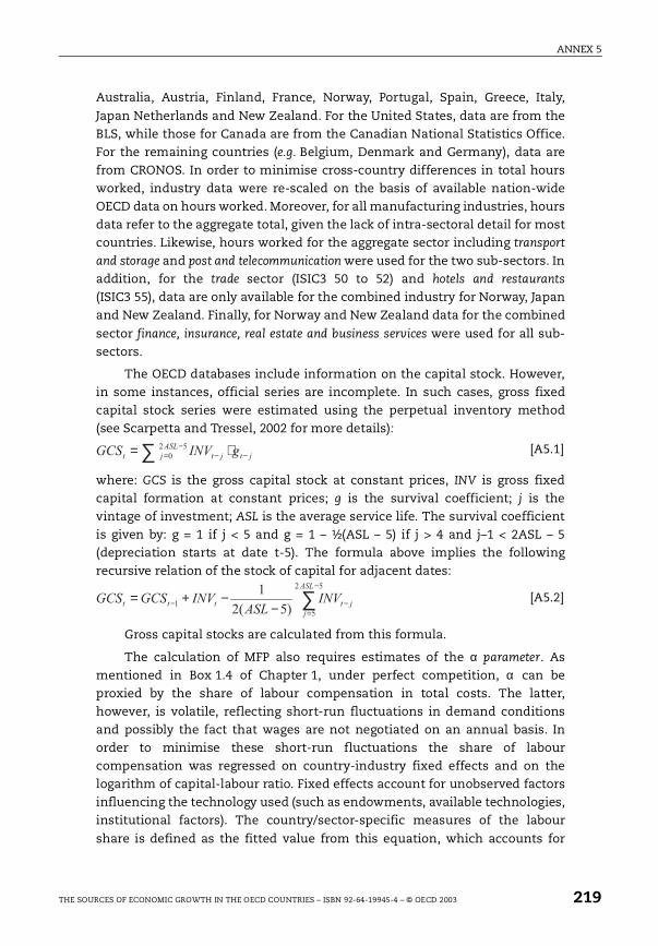
ANNEX 5
Australia, Austria, Finland, France, Norway, Portugal, Spain, Greece, Italy,
Japan Netherlands and New Zealand. For the United States, data are from theBLS, while those for Canada are from the Canadian National Statistics Office.For the remaining countries (e.g. Belgium, Denmark and Germany), data arefrom CRONOS. In order to minimise cross-country differences in total hoursworked, industry data were re-scaled on the basis of available nation-wideOECD data on hours worked. Moreover, for all manufacturing industries, hoursdata refer to the aggregate total, given the lack of intra-sectoral detail for mostcountries. Likewise, hours worked for the aggregate sector including transport
and storage and post and telecommunication were used for the two sub-sectors. Inaddition, for the trade sector (ISIC3 50 to 52) and hotels and restaurants
(ISIC3 55), data are only available for the combined industry for Norway, Japanand New Zealand. Finally, for Norway and New Zealand data for the combined
sector finance, insurance, real estate and business services were used for all sub-sectors.
The OECD databases include information on the capital stock. However,in some instances, official series are incomplete. In such cases, gross fixedcapital stock series were estimated using the perpetual inventory method(see Scarpetta and Tressel, 2002 for more details):
where: GCS is the gross capital stock at constant prices, INV is gross fixedcapital formation at constant prices; g is the survival coefficient; j is thevintage of investment; ASL is the average service life. The survival coefficientis given by: g = 1 if j < 5 and g = 1 – ½(ASL – 5) if j > 4 and j–1 < 2ASL – 5(depreciation starts at date t-5). The formula above implies the followingrecursive relation of the stock of capital for adjacent dates:
Gross capital stocks are calculated from this formula.
The calculation of MFP also requires estimates of the α parameter. Asmentioned in Box 1.4 of Chapter 1, under perfect competition, α can beproxied by the share of labour compensation in total costs. The latter,however, is volatile, reflecting short-run fluctuations in demand conditionsand possibly the fact that wages are not negotiated on an annual basis. Inorder to minimise these short-run fluctuations the share of labourcompensation was regressed on country-industry fixed effects and on thelogarithm of capital-labour ratio. Fixed effects account for unobserved factorsinfluencing the technology used (such as endowments, available technologies,institutional factors). The country/sector-specific measures of the labour
share is defined as the fitted value from this equation, which accounts for
∑ −−−
= ⋅= jtjt
ASL
jt gINVGCS 52
0[A5.1]
∑−
=−− −
−+=52
5
1)5(2
1 ASL
j
jtttt INVASL
INVGCSGCS [A5.2]
THE SOURCES OF ECONOMIC GROWTH IN THE OECD COUNTRIES – ISBN 92-64-19945-4 – © OECD 2003 219
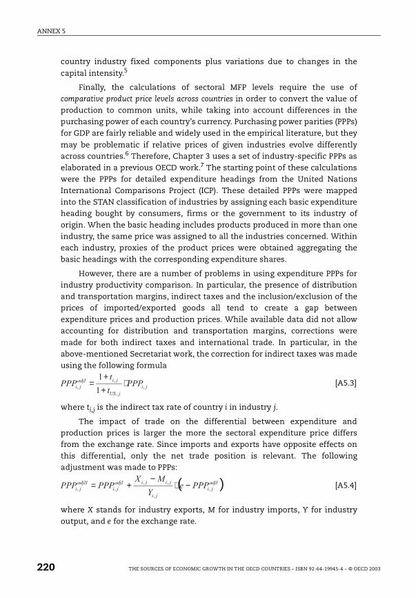
ANNEX 5
country industry fixed components plus variations due to changes in the
capital intensity.5
Finally, the calculations of sectoral MFP levels require the use ofcomparative product price levels across countries in order to convert the value ofproduction to common units, while taking into account differences in thepurchasing power of each country’s currency. Purchasing power parities (PPPs)for GDP are fairly reliable and widely used in the empirical literature, but they
may be problematic if relative prices of given industries evolve differentlyacross countries.6 Therefore, Chapter 3 uses a set of industry-specific PPPs aselaborated in a previous OECD work.7 The starting point of these calculationswere the PPPs for detailed expenditure headings from the United NationsInternational Comparisons Project (ICP). These detailed PPPs were mappedinto the STAN classification of industries by assigning each basic expenditureheading bought by consumers, firms or the government to its industry oforigin. When the basic heading includes products produced in more than oneindustry, the same price was assigned to all the industries concerned. Withineach industry, proxies of the product prices were obtained aggregating thebasic headings with the corresponding expenditure shares.
However, there are a number of problems in using expenditure PPPs forindustry productivity comparison. In particular, the presence of distributionand transportation margins, indirect taxes and the inclusion/exclusion of theprices of imported/exported goods all tend to create a gap betweenexpenditure prices and production prices. While available data did not allowaccounting for distribution and transportation margins, corrections were
made for both indirect taxes and international trade. In particular, in theabove-mentioned Secretariat work, the correction for indirect taxes was madeusing the following formula
where ti,j is the indirect tax rate of country i in industry j.
The impact of trade on the differential between expenditure andproduction prices is larger the more the sectoral expenditure price differsfrom the exchange rate. Since imports and exports have opposite effects onthis differential, only the net trade position is relevant. The followingadjustment was made to PPPs:
where X stands for industry exports, M for industry imports, Y for industryoutput, and e for the exchange rate.
ji
jUS
jiadjI
ji PPPt
tPPP ,
,
,
,1
1⋅
++
= [A5.3]
( )adjI
ji
ji
jijiadjI
ji
adjII
ji PPPeY
MXPPPPPP ,
,
,,
,, −⋅−
+= [A5.4]
220 THE SOURCES OF ECONOMIC GROWTH IN THE OECD COUNTRIES – ISBN 92-64-19945-4 – © OECD 2003
ANNEX 5
Other Variables used in the industry-level analysis
Data on R&D intensity are drawn from the OECD ANBERD database. R&Dintensity is defined as the ratio of Business Expenditure in Research andDevelopment (BERD) to value-added. Value-added is from the main data-setdiscussed above.
Different measures of human capital were considered. First, macro-economic proxy for general human capital, such as the proportion ofindividual with secondary school attainment and the average number of yearsof schooling were considered (see Bassanini and Scarpetta, 2001). Contrary toGriffith et al. (2000), the coefficients on either of these two variables turned outto be statistically insignificant in MFP regressions. The second measure was
an industry-level proxy of human capital, based on the skill composition ofemployment and relative wages by skill level. Thus, the measure of humancapital was defined by (the subscripts j, i and t are omitted):
where ωHWh, ωLWh, ωHBl, ωLBl are respectively the wage rate for the white-collarhigh-skill, white-collar low-skill, blue-collar high-skill and blue-collar low-skill workers. LHWh, LHBl and L are respectively white-collar high-skill
employment, blue-collar high skill employment and total employment. Thus,this measure is rising with the wage premium of (white-collar and blue-collar)skilled workers relative to unskilled workers, weighted with the proportion of(white-collar and blue-collar) skilled workers in total employment.
In the next step, this variable is regressed on: 1) country-specific andindustry-specific fixed effects; and 2) time dummies that are country and
industry specific. The predicted value is used as a measure of human capitalin the MFP regressions reported in the main text.8
All the economy-wide and sector-specific indicators of the stringency ofproduct market regulations are from the OECD International Regulation Database
(see Nicoletti et al., 1999), except for the time-varying summary indicator ofregulation that has been constructed from industry-level data (see Nicoletti et
al., 2001). In particular, the sectoral indicators cover energy and marketableservice industries at the 3 or 4-digit level of ISIC Rev 3 classification (a total of21 industries and industry aggregates) in (or around 1998) and, the time-varying indicator focuses on seven of them, over the 1975-1998 period.Depending on the industry, the resulting dataset covers barriers to entry,public ownership, price controls, government involvement in businessoperation, market concentration and vertical integration. In networkindustries – such as utilities, post and telecommunications and railways – thebasic data concerned regulatory and market conditions in different (vertical orhorizontal) segments of the industries (e.g. gas production, distribution and
++=
L
L
L
LalHumanCapit HBl
LBl
HBlHWh
LWh
HWh ..1logωω
ωω
[A5.5]
THE SOURCES OF ECONOMIC GROWTH IN THE OECD COUNTRIES – ISBN 92-64-19945-4 – © OECD 2003 221
ANNEX 5
supply, or regular and express mail). The main sources used to collect the data
are the following:9
the OECD: Regulatory Reform, Privatisation and Competition Policy (1992);The OECD International Regulation Database; OECD Roundtables oncompetition and regulation, various issues; OECD Reviews of RegulatoryReform, various issues; OECD Economic Studies, No. 32 (2001) (andbackground OECD Economics Department Working Papers Nos. 251, 237,
238, 254, 255); OECD Report on Regulatory Reform (1997).
the European Conference of Ministers of Transportation: Rail Restructuringin Europe (1998); Regulatory Reforms in the Transport Sector (1987);Competition Policy and Deregulation of Road Transport (1990); RailwayReform (2001);
the World Bank: Industry Structure and Regulation in Infrastructure: aCross-Country Survey (1996);
the European Commission: Liberalisation of Network Industries (1999) (andbackground documents); Green Paper on Postal Services (1993)
Center for the Study of Regulated Industries/Privatisation International:I. Lewington (ed.), Utility Regulation (1997);
Australian Productivity Commission: G. McGuire, M. Schuele and Smith,“Restrictiveness of international trade in maritime services”, Productivity
Commission Staff Research Paper (2000); K. Kalijaran, “Restrictions on trade inbusiness services”, Productivity Commission Staff Research Paper (2000);D. Nguyen-Hong, “Restrictions on trade in professional services”,Productivity Commission Staff Research Paper (2000); Trade and Assistance
Review 1998-99 (1999).
Further details about coverage and sources in each of the industriesincluded in the analysis are provided in Table A5.6 and in Nicoletti et al., 2001.
As for the nation-wide indicators of regulations, regulatory indicators byindustry were based on basic cross-country data ordered according to thefriendliness of regulations, market structures and industry structures tocompetition. The resulting cardinal indicators were re-scaled to ensure thecomparability of the product market indicators across industries. The aim ofthis operation was to account for structural differences in industrycharacteristics, such as differences in minimum efficiency scale or verticaland horizontal relationships.10 For each regulatory and market dimensioncovered in the dataset, cross-country indicators at the two-digit (ISIC Rev. 3)
industry level were constructed by weighting the indices for lower-digitindustries with average OECD employment shares. Finally, summaryindicators of product market regulation by industry were derived taking thesimple average of the regulatory dimensions covered in each industry.11
222 THE SOURCES OF ECONOMIC GROWTH IN THE OECD COUNTRIES – ISBN 92-64-19945-4 – © OECD 2003
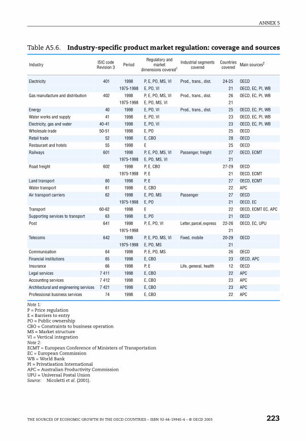
ANNEX 5
ces
APC
Table A5.6. Industry-specific product market regulation: coverage and sour
Note 1:P = Price regulationE = Barriers to entryPO = Public ownershipCBO = Constraints to business operationMS = Market structureVI = Vertical integrationNote 2:ECMT = European Conference of Ministers of TransportationEC = European CommissionWB = World BankPI = Privatisation InternationalAPC = Australian Productivity CommissionUPU = Universal Postal UnionSource: Nicoletti et al. (2001).
Industry ISIC code Revision 3 Period
Regulatory and market
dimensions covered1
Industrial segments covered
Countries covered Main sources2
Electricity 401 1998 P, E, PO, MS, VI Prod., trans., dist. 24-25 OECD
1975-1998 E, PO, VI 21 OECD, EC, PI, WB
Gas manufacture and distribution 402 1998 P, E, PO, MS, VI Prod., trans., dist. 26 OECD, EC, PI, WB
1975-1998 E, PO, MS, VI 21
Energy 40 1998 E, PO, VI Prod., trans., dist. 25 OECD, EC, PI, WB
Water works and supply 41 1998 E, PO, VI 23 OECD, EC, PI, WB
Electricity, gas and water 40-41 1998 E, PO, VI 23 OECD, EC, PI, WB
Wholesale trade 50-51 1998 E, PO 25 OECD
Retail trade 52 1998 E, CBO 28 OECD
Restaurant and hotels 55 1998 E 25 OECD
Railways 601 1998 P, E, PO, MS, VI Passenger, freight 27 OECD, ECMT
1975-1998 E, PO, MS, VI 21
Road freight 602 1998 P, E, CBO 27-29 OECD
1975-1998 P, E 21 OECD, ECMT
Land transport 60 1998 P, E 27 OECD, ECMT
Water transport 61 1998 E, CBO 22 APC
Air transport carriers 62 1998 E, PO, MS Passenger 27 OECD
1975-1998 E, PO 21 OECD, EC
Transport 60-62 1998 E 22 OECD, ECMT EC,
Supporting services to transport 63 1998 E, PO 21 OECD
Post 641 1998 P, E, PO, VI Letter, parcel, express 22-26 OECD, EC, UPU
1975-1998 21
Telecoms 642 1998 P, E, PO, MS, VI Fixed, mobile 20-29 OECD
1975-1998 E, PO, MS 21
Communication 64 1998 P, E, PO, MS 26 OECD
Financial institutions 65 1998 E, CBO 23 OECD, APC
Insurance 66 1998 P, E Life, general, health 12 OECD
Legal services 7 411 1998 E, CBO 22 APC
Accounting services 7 412 1998 E, CBO 23 APC
Architectural and engineering services 7 421 1998 E, CBO 23 APC
Professional business services 74 1998 E, CBO 22 APC
THE SOURCES OF ECONOMIC GROWTH IN THE OECD COUNTRIES – ISBN 92-64-19945-4 – © OECD 2003 223
ANNEX 5
The time-varying indicator of product market regulations was obtained
by using data on regulatory and market developments over the 1970-1998 period in seven energy and service industries: gas, electricity, post,telecommunications (mobile and fixed services), passenger air transport,railways (passenger and freight services) and road freight (see Nicoletti et al.,2001). The coverage of regulatory areas varies across industries. Regulatorybarriers to entry are reported for all industries; public ownership is reported in allindustries except road freight; vertical integration is documented for gas,electricity and railways; market structure is documented for gas,telecommunications and railways; and price controls are reported for roadfreight. The aggregate time-series indicator of regulation was constructed bytaking a simple average of the summary indicators for the seven industries.The resulting indicators were interpreted as a proxy for the overall regulatory
policies followed by OECD countries over the sample period.
A5.4. Chapter 4 : Firm-level data
The data and methods used in the productivity decompositions andanalysis of firm dynamics presented in Chapter 4 were built within thecontext of the OECD firm-level project, involving ten countries (Canada,
Denmark, France, Finland, Germany, Italy, the Netherlands, Portugal, theUnited Kingdom, and the United States). These data and methods aredescribed in Annex 4 above. Further details are contained in Tables A5.7and A5.8.12
Notes
1. The estimates of gross capital stock were based on BEA’s former gross stockmeasure up to 1993, the last available update. More recent estimates wereobtained as follows: the historical series of gross stock were regressed againstBEA’s net stock series and BLS’ capital services series. For years after 1993, thegross stock was then estimated as the predicted value from this regression, usingrecent observations on the net stock and on capital services.
2. De la Fuente and Doménech (2000) revised the original series from Barro and Lee(1996) to eliminate anomalies in connection with attainment rates.
3. Chemicals excluding Pharmaceuticals, Pharmaceutical, Building and Repairing ofShips and Boats, Aircraft and Spacecraft, Railroad Equipment and TransportEquipment N.E.C.
4. For a sensitivity analysis of the empirical results of Chapter 4 using alternativeestimates of labour input, see Scarpetta and Tressel (2002).
5. For a sensitivity analysis of the empirical results of Chapter 3 using alternativeestimates of the labour share, see Scarpetta and Tressel (2002).
6. For example, Sørensen (2001) shows that aggregate PPPs may be somewhatproblematic to study country convergence in manufacturing productivity. Indeed,while relative productivity levels are independent of the choice of the base year,
224 THE SOURCES OF ECONOMIC GROWTH IN THE OECD COUNTRIES – ISBN 92-64-19945-4 – © OECD 2003
ANNEX 5
using PPPs for total GDP leads to different degree of convergence depending on thebase year chosen for PPPs. This may be due to the fact that relative prices ofmanufacturing have evolved differently across countries, but may also reflect thefact that PPPs for total GDP have improved over time. See also Schreyer and Pilat(2001) for a discussion on these issues.
7. These data are available upon request. For a sensitivity analysis of the empiricalresults of Chapter 3 using alternative (i.e. aggregate) measures of PPPs,see Scarpetta and Tressel (2002).
8. The coefficient remains significant with the same sign if the original variable isused instead of the predicted one in the productivity regressions. The use of theoriginal variable, however, reduces somewhat the sample size, and thus it wasdecided to use the predicted human capital variable.
9. Other sources include the International Energy Agency, the Universal Postal Unionand the National Economic Research Associates.
10. For instance, indicators for barriers to entry in each industry were rescaled usingthe OECD average of the frequency of barriers to entry in that industry. As a result,indicators of barriers to entry in structurally competitive industries (such as retaildistribution) take by construction a lower range of values than indicators ofbarriers to entry in industries having natural monopoly elements (such aselectricity).
11. Unlike the economy-wide indicators of product market regulation, thedimensions available for time-series data were too few to be able to aggregatedetailed indicators by means of factor analysis.
12. For an overview of the issues encountered in the use of firm-level data and detailson the subsequent research protocol, see Scarpetta et al. (2002).
THE SOURCES OF ECONOMIC GROWTH IN THE OECD COUNTRIES – ISBN 92-64-19945-4 – © OECD 2003 225
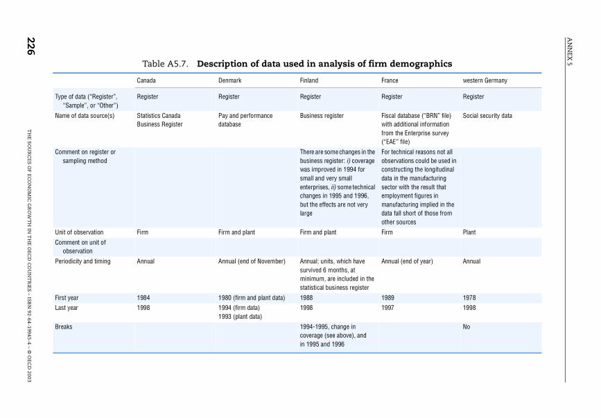
AN
NEX
5
226T
HE S
OU
RC
ES O
F EC
ON
OM
IC G
RO
WT
H IN
TH
E OEC
D C
OU
NT
RIES – ISB
N 92-64-19945-4 – ©
OEC
D 2003
firm demographics
France western Germany
Register Register
Fiscal database (“BRN” file) with additional information from the Enterprise survey (“EAE” file)
Social security data
the ge
cal ,
For technical reasons not all observations could be used in constructing the longitudinal data in the manufacturing sector with the result that employment figures in manufacturing implied in the data fall short of those from other sources
Firm Plant
he
Annual (end of year) Annual
1989 1978
1997 1998
No
Table A5.7. Description of data used in analysis of
Canada Denmark Finland
Type of data (“Register”, “Sample”, or “Other”)
Register Register Register
Name of data source(s) Statistics Canada Business Register
Pay and performance database
Business register
Comment on register or sampling method
There are some changes in business register: i) coverawas improved in 1994 for small and very small enterprises, ii) some technichanges in 1995 and 1996but the effects are not verylarge
Unit of observation Firm Firm and plant Firm and plant
Comment on unit of observation
Periodicity and timing Annual Annual (end of November) Annual: units, which have survived 6 months, at minimum, are included in tstatistical business register
First year 1984 1980 (firm and plant data) 1988
Last year 1998 1994 (firm data) 1993 (plant data)
1998
Breaks 1994-1995, change in coverage (see above), and in 1995 and 1996
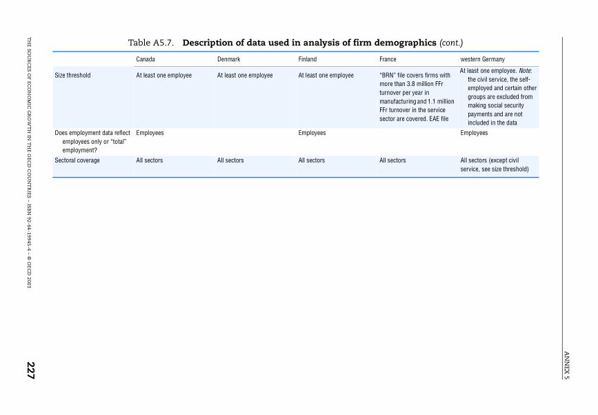
AN
NEX
5
TH
E SOU
RC
ES OF EC
ON
OM
IC G
RO
WT
H IN
TH
E OEC
D C
OU
NT
RIES
– ISB
N 92-64-19945-4 – ©
OE
CD
2003227
Table A5.7. Description of data used in analysis of firm demographics (cont.)
France western Germany
“BRN” file covers firms with more than 3.8 million FFr turnover per year in manufacturing and 1.1 million FFr turnover in the service sector are covered. EAE file
At least one employee. Note: the civil service, the self-employed and certain other groups are excluded from making social security payments and are not included in the data
Employees
All sectors All sectors (except civil service, see size threshold)
Canada Denmark Finland
Size threshold At least one employee At least one employee At least one employee
Does employment data reflect employees only or “total” employment?
Employees Employees
Sectoral coverage All sectors All sectors All sectors
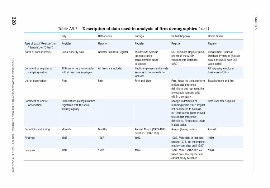
AN
NEX
5
228T
HE S
OU
RC
ES O
F EC
ON
OM
IC G
RO
WT
H IN
TH
E OEC
D C
OU
NT
RIES – ISB
N 92-64-19945-4 – ©
OEC
D 2003
demographics (cont.)
United Kingdom United States
Register Register
CSO Business Register [also known as the ACOP Respondents Database (ARD)]
Longitudinal Business Database Prototype (Source data is the SSEL with CES value added)
te
All taxpaying employer businesses (EINs)
Firm. Note: the units conform to Eurostat enterprise definitions and represent the lowest autonomous units within a company
Establishment and firm
Change in definition of reporting unit in 1987. Impact not considered to be large. In 1994: New register, moved to Eurostat enterprise definitions. Almost total break in data series
Firm level data supplied
), Annual (timing varies) Annual
1980. Note: data in fact date back to 1973, but incomplete employment data until 1980)
1989
1992. Note: 1994-1997 are based on a new register and cannot easily be linked
1996
Table A5.7. Description of data used in analysis of firm
Italy Netherlands Portugal
Type of data (“Register”, or “Sample”, or “Other”)
Register Register Register
Name of data source(s) Social security data General Business Register Quadros do pessoal (administrative establishment-based database)
Comment on register or sampling method
All firms in the private sector with at least one employee
All firms are included Public employees and privaservices to households notincluded
Unit of observation Firm Firm Firm and plant
Comment on unit of observation
Observations are legal entities registered with the social security agency.
Periodicity and timing Monthly Monthly Annual. March (1983-1993October (1994-1998)
First year 1986 1987 1983
Last year 1994 1997 1994
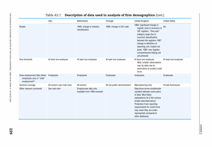
AN
NEX
5
TH
E SOU
RC
ES OF EC
ON
OM
IC G
RO
WT
H IN
TH
E OEC
D C
OU
NT
RIES
– ISB
N 92-64-19945-4 – ©
OE
CD
2003229
Table A5.7. Description of data used in analysis of firm demographics (cont.)
United Kingdom United States
1984: significant change in register (due to inclusion of VAT register). “One-year” category large due to incorrect classification between the registers 1987: change in definition of reporting unit, impact not great. 1994: new register, comprehensive linking not yet achieved
No
At least one employee. Note: smaller observations may be older due to restrictions to protect small firms
At least one employee
Employees Employees
n Manufacturing only Private businesses
Data show some considerable variation between some years of data. Most likely explanations lie in the various breaks described above. Protection from reporting requirements for small firms may mean they are under-represented compared to other databases
Italy Netherlands Portugal
Breaks 1993: change in industry classification
1995: change in SIC code
Size threshold At least one employee At least one employee At least one employee
Does employment data reflect employees only or “total” employment?
Employees Employees Employees
Sectoral coverage All sectors (see main text) All sectors All but public administratio
Other relevant comments See main text Employment data only available from 1993 onwards
AN
NEX
5
230T
HE S
OU
RC
ES O
F EC
ON
OM
IC G
RO
WT
H IN
TH
E OEC
D C
OU
NT
RIES – ISB
N 92-64-19945-4 – ©
OEC
D 2003
demographics (cont.)
time. In order to prevent this expansion being reflected asg in the data fall short of those from other sources; althoughography.
gers and acquisitions. For entry, the date registered is whencide to employ individuals on an official basis. Mergers and
portance in certain regions and sectors. According to someof legal status, 20 per cent involves a substantial change of In addition, there are some minor problems in conforminggh most matches are accurate, some are more problematic. nec”. The Ateco81 sector “Measurement and Telecomm. the production and repair and maintenance of computingpart of it should be attributed to business services.
1989 to 1993). It should be noted that early years of the dataluding register and changes in reporting unit. For the more aggregate terms the employment data from the UK micro
993 and increases to about 85 000 in 1986.
Table A5.7. Description of data used in analysis of firm
Supplementary notes:France:The register for the manufacturing sector has expanded to cover an increasing number of businesses overfirm entries, only a subset of the register data are used. As a result the employment figures for manufacturinthey are still be representative with regard to the productivity decompositions and the analysis of firm demItaly:Two issues are worth noting about the nature of entries and the extent to which entries and exits reflect merthe first hiring occurs. Thus, for example, the “entries” may reflect cases where (usually small) enterprises deacquisitions cannot be identified across the data as whole, but there has been some estimation of their imstudies using INPS data for particular regions and periods: between 10 and 15 per cent of entry is a change pre-existing firms, and 65-70 per cent is “pure” entry (equivalent figures are likely to hold for exiting firms).to the OECD STAN sector classification. The INPS data are based on the Italian classification Ateco81: althouThe Ateco81 sector “Metals and machinery nec”, is attributed to the STAN “Machinery and EquipmentEquipment”, is placed in the STAN sector “Communication Equipment”. Ateco81 330, which includes bothmachines, is attributed to the STAN “Office, accounting and computing equipment”, even though in theory The United Kingdom:The analysis of firm demographics for the United Kingdom uses data for the end of the time span covered (show some large changes in the number of firms over time.1 These are attributable to a variety of factors increcent years of available data the sectoral distribution of the firm-level data is considered representative. Indata is slightly below the reported employment for UK manufacturing, and this is consistent over time.1. For example, the total number of continuing firms falls from around 75 000 to 20 000 between 1982 and 1Source: OECD.
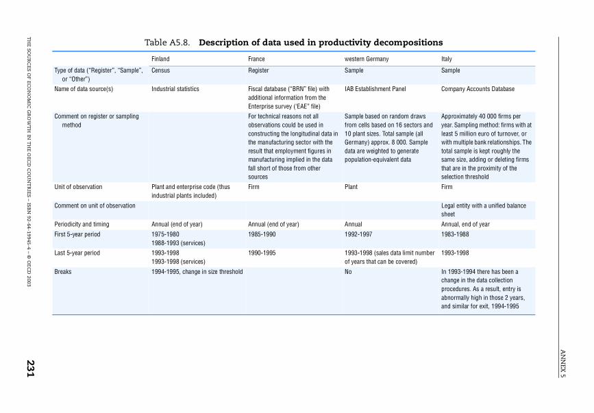
AN
NEX
5
TH
E SOU
RC
ES OF EC
ON
OM
IC G
RO
WT
H IN
TH
E OEC
D C
OU
NT
RIES
– ISB
N 92-64-19945-4 – ©
OE
CD
2003231
Table A5.8. Description of data used in productivity decompositions
Germany Italy
Sample
ablishment Panel Company Accounts Database
based on random draws lls based on 16 sectors and t sizes. Total sample (all y) approx. 8 000. Sample weighted to generate ion-equivalent data
Approximately 40 000 firms per year. Sampling method: firms with at least 5 million euro of turnover, or with multiple bank relationships. The total sample is kept roughly the same size, adding or deleting firms that are in the proximity of the selection threshold
Firm
Legal entity with a unified balance sheet
Annual, end of year
997 1983-1988
998 (sales data limit number that can be covered)
1993-1998
In 1993-1994 there has been a change in the data collection procedures. As a result, entry is abnormally high in those 2 years, and similar for exit, 1994-1995
Finland France western
Type of data (“Register”, “Sample”, or “Other”)
Census Register Sample
Name of data source(s) Industrial statistics Fiscal database (“BRN” file) with additional information from the Enterprise survey (‘EAE” file)
IAB Est
Comment on register or sampling method
For technical reasons not all observations could be used in constructing the longitudinal data in the manufacturing sector with the result that employment figures in manufacturing implied in the data fall short of those from other sources
Samplefrom ce10 planGermandata arepopulat
Unit of observation Plant and enterprise code (thus industrial plants included)
Firm Plant
Comment on unit of observation
Periodicity and timing Annual (end of year) Annual (end of year) Annual
First 5-year period 1975-19801988-1993 (services)
1985-1990 1992-1
Last 5-year period 1993-19981993-1998 (services)
1990-1995 1993-1of years
Breaks 1994-1995, change in size threshold No
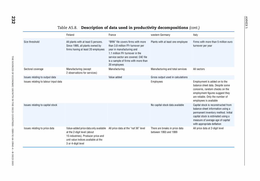
AN
NEX
5
232T
HE S
OU
RC
ES O
F EC
ON
OM
IC G
RO
WT
H IN
TH
E OEC
D C
OU
NT
RIES – ISB
N 92-64-19945-4 – ©
OEC
D 2003
ecompositions (cont.)
Germany Italy
ith at least one employee Firms with more than 5 million euro turnover per year
cturing and total services All sectors
utput used in calculations
ees Employment is added on to the balance sheet data. Despite some concerns, random checks on the employment figures suggest they are reliable. Only the number of employees is available
tal stock data available Capital stock is reconstructed from balance sheet information using a permanent inventory method. Initial capital stock is estimated using a measure of average age of capital with appropriate deflation
re breaks in price data 1993 and 1999
All price data at 2-digit level
Table A5.8. Description of data used in productivity d
Finland France western
Size threshold All plants with at least 5 persons. Since 1995, all plants owned by firms having at least 20 employees
“BRN” file covers firms with more than 3.8 million FFr turnover per year in manufacturing and 1.1 million FFr turnover in the service sector are covered. EAE file is a sample of firms with more than 20 employees
Plants w
Sectoral coverage Manufacturing (except 2 observations for services)
Manufacturing Manufa
Issues relating to output data Value added Gross o
Issues relating to labour input data Employ
Issues relating to capital stock No capi
Issues relating to price data Value-added price data only available at the 2-digit level (about 15 industries). Producer price and unit value indices available at the 3 or 4-digit level
All price data at the “naf 36” level There abetween
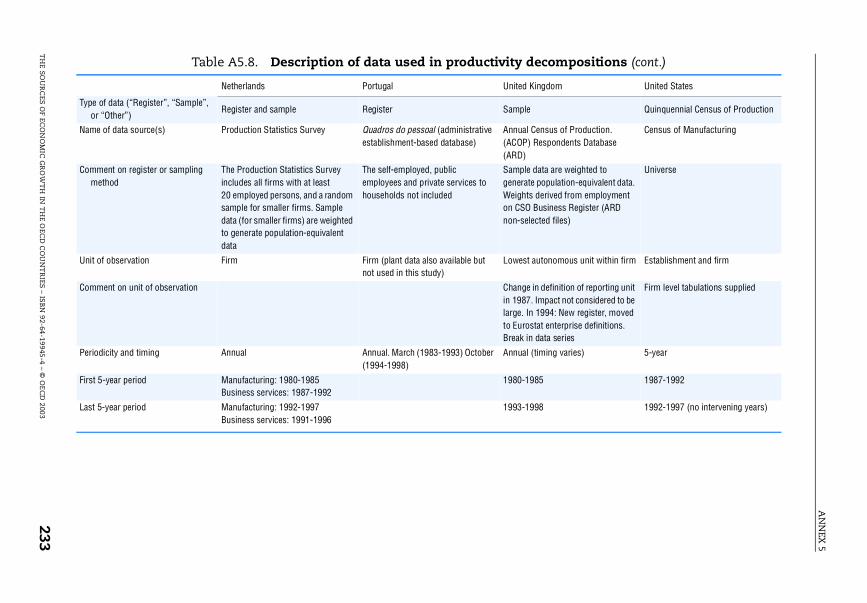
AN
NEX
5
TH
E SOU
RC
ES OF EC
ON
OM
IC G
RO
WT
H IN
TH
E OEC
D C
OU
NT
RIES
– ISB
N 92-64-19945-4 – ©
OE
CD
2003233
Table A5.8. Description of data used in productivity decompositions (cont.)
ingdom United States
Quinquennial Census of Production
Census of Production. Respondents Database
Census of Manufacturing
data are weighted to e population-equivalent data. derived from employment Business Register (ARD ected files)
Universe
autonomous unit within firm Establishment and firm
in definition of reporting unit . Impact not considered to be
1994: New register, moved stat enterprise definitions. data series
Firm level tabulations supplied
(timing varies) 5-year
985 1987-1992
998 1992-1997 (no intervening years)
Netherlands Portugal United K
Type of data (“Register”, “Sample”, or “Other”)
Register and sample Register Sample
Name of data source(s) Production Statistics Survey Quadros do pessoal (administrative establishment-based database)
Annual (ACOP)(ARD)
Comment on register or sampling method
The Production Statistics Survey includes all firms with at least 20 employed persons, and a random sample for smaller firms. Sample data (for smaller firms) are weighted to generate population-equivalent data
The self-employed, public employees and private services to households not included
SamplegeneratWeightson CSOnon-sel
Unit of observation Firm Firm (plant data also available but not used in this study)
Lowest
Comment on unit of observation Changein 1987large. Into EuroBreak in
Periodicity and timing Annual Annual. March (1983-1993) October (1994-1998)
Annual
First 5-year period Manufacturing: 1980-1985Business services: 1987-1992
1980-1
Last 5-year period Manufacturing: 1992-1997Business services: 1991-1996
1993-1
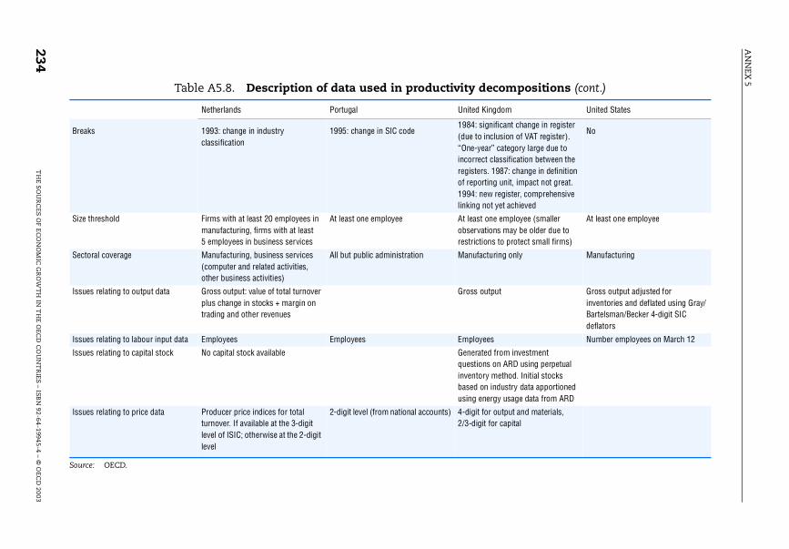
AN
NEX
5
234T
HE S
OU
RC
ES O
F EC
ON
OM
IC G
RO
WT
H IN
TH
E OEC
D C
OU
NT
RIES – ISB
N 92-64-19945-4 – ©
OEC
D 2003
ecompositions (cont.)
ingdom United States
ignificant change in register inclusion of VAT register). ar” category large due to t classification between the s. 1987: change in definition ting unit, impact not great. ew register, comprehensive not yet achieved
No
one employee (smaller tions may be older due to ons to protect small firms)
At least one employee
cturing only Manufacturing
utput Gross output adjusted for inventories and deflated using Gray/Bartelsman/Becker 4-digit SIC deflators
ees Number employees on March 12
ed from investment ns on ARD using perpetual ry method. Initial stocks n industry data apportioned nergy usage data from ARD
or output and materials, it for capital
Table A5.8. Description of data used in productivity d
Source: OECD.
Netherlands Portugal United K
Breaks 1993: change in industry classification
1995: change in SIC code1984: s(due to “One-yeincorrecregisterof repor1994: nlinking
Size threshold Firms with at least 20 employees in manufacturing, firms with at least 5 employees in business services
At least one employee At leastobservarestricti
Sectoral coverage Manufacturing, business services (computer and related activities, other business activities)
All but public administration Manufa
Issues relating to output data Gross output: value of total turnover plus change in stocks + margin on trading and other revenues
Gross o
Issues relating to labour input data Employees Employees Employ
Issues relating to capital stock No capital stock available Generatquestioinventobased ousing e
Issues relating to price data Producer price indices for total turnover. If available at the 3-digit level of ISIC; otherwise at the 2-digit level
2-digit level (from national accounts) 4-digit f2/3-dig
BIBLIOGRAPHY
Bibliography
AARON, H.J. (1990),“Discussion of “Why is Infrastructure Important’?” in: A.H. Munnel (ed.), Is There aShortfall in Public Capital Investment?, Federal Reserve Bank of Boston, Boston,pp. 21-68.
ACEMOGLU, D. and S. PISCHKE (1999a),“The Structure of Wages and Investment in General Training”, Journal of PoliticalEconomy, Vol. 107, pp. 539-572.
ACEMOGLU, D. and S. PISCHKE (1999b),“Beyond Becker: Training in Imperfect Labor Markets”, Economic Journal, Vol. 109,No. 453, pp. F112-142.
AGHION, P. and P. HOWITT (1992),“A Model of Growth through Creative Destruction”, Econometrica, Vol. 60,pp. 323-51.
AGHION, P. and P. HOWITT (1998),Endogenous Growth Theory, The MIT Press, Cambridge, Mass.
AGHION, P., C. HARRIS, P. HOWITT and J. VICKERS (2001a),“Competition, Imitation and Growth with Step-by-Step Innovation”, Review ofEconomic Studies, Vol. 68, pp. 467-492.
AGHION, P., N. BLOOM, R. BLUNDELL, R. GRIFFITH and P. HOWITT (2001b),“Empirical Estimates of Product Market Competition and Innovation”, UniversityCollege London, London, mimeo.
AHN, S. and P. HEMMINGS (2000),“Policy Influences on Economic Growth in OECD Countries: an Evaluation of theEvidence”, OECD Economics Department Working Papers, No. 246.
AHN, S. (2001),“Firm Dynamics and Productivity Growth: A Review of Micro Evidence for theOECD Countries”, OECD Economics Department Working Papers, No. 297.
AKERLOF, G.A., W.T. DICKENS and G.L. PERRY. (1996),“The Macroeconomics of Low Inflation”, Brookings Papers on Economic Activity,Vol. 1, pp. 1-59.
ALEXANDER, R.J. (1997),“Inflation and Economic Growth: Evidence from a Growth Equation”, AppliedEconomics, Vol. 29, No. 2, pp. 233-38.
ANDRES, J. and I. HERNANDO (1997),“Does Inflation Harm Economic Growth? Evidence for the OECD”, NBER WorkingPaper, No. 6062.
THE SOURCES OF ECONOMIC GROWTH IN THE OECD COUNTRIES – ISBN 92-64-19945-4 – © OECD 2003 235
BIBLIOGRAPHY
APEL, M. and P. JANSSON (1999),“A Theory-Consistent Approach for Estimating Potential Output and the NAIRU”,Economics Letters, No. 74, pp. 271-75.
ARK, B. VAN (1996),“Sectoral Growth Accounting and Structural Change in Post-War Europe”, in:B. Van Ark and N.F.R. Crafts, (eds), Quantitative Aspects of Post-War EuropeanEconomic Growth, CEPR/Cambridge University Press, Cambridge, Mass., pp. 84-164.
ARNAL, E.W. OK, R. TORRES (2001),“Knowledge, Work Organisation and Economic Growth”, OECD DEELSA OccasionalPapers, No. 50.
ARROW, K.J. (1962),“The Economic Implications of Learning by Doing”, Review of Economic Studies,Vol. 29, pp. 155-73.
ASCHAUER, D.A. (1989),“Is Public Expenditure Productive?”, Journal of Monetary Economics, Vol. 23,pp. 177-200.
AUDRETSCH, D.B. (1995a),Innovation and Industry Evolution, MIT Press, Cambridge, Mass.
AUDRETSCH, D.B. (1995b),“Innovation, Survival and Growth”, International Journal of Industrial Organization,Vol. 13, pp. 441-457.
AUDRETSCH, D.B. and T. MAHMOOD (1994),“The Rate of Hazard Confronting New Firms and Plants in US Manufacturing”,Review of Industrial Organization, Vol. 9, pp. 41-56.
AUDRETSCH, D.B. and R. THURIK (2001),“Linking Entrepreneurship to Growth”, OECD STI Working Papers, No. 2001/2.
BAILY, M.N., E.J. BARTELSMAN and J. HALTIWANGER (1996),“Downsizing and Productivity Growth: Myth or Reality?” Small Business Economics,Vol. 8, pp. 259-278.
BAILY, M.N., E.J. BARTELSMAN and J. HALTIWANGER (1997),“Labor Productivity: Structural Change and Cyclical Dynamics”, NBER WorkingPaper, No. 5503.
BAILY, M.N., C. HULTEN and D. CAMPBELL (1992),“Productivity Dynamics in Manufacturing Plants”, Brookings Papers on EconomicsActivity: Microeconomics, Vol. 2, pp. 187-249.
BALDWIN, J.R. and P.K. GORECKI (1991),“Entry, Exit, and Productivity Growth”, in: P.A. Geroski and J. Schwalbach (eds.),Entry and Market Contestability: An International Comparison, Blackwell, Oxford.
BALL, L. and S.G. CECCHETTI (1990),“Inflation and Uncertainty at Short and Long Horizons”, Brookings Papers onEconomic Activity, Vol. 1, pp. 215-245.
BARRO, R.J. (1976),“Rational Expectations and the Role of Monetary Policy”, Journal of MonetaryEconomics, Vol. 2, pp. 1-32.
236 THE SOURCES OF ECONOMIC GROWTH IN THE OECD COUNTRIES – ISBN 92-64-19945-4 – © OECD 2003
BIBLIOGRAPHY
BARRO, R.J. (1980),“A Capital Market Equilibrium Business Cycle Model”, Econometrica, Vol. 48, No. 6,pp. 1393-1417.
BARRO, R.J. (1990),“Government Spending in a Simple Model of Endogenous Growth”, Journal ofPolitical Economy, Vol. 98, No. 5, pp. S103-S125.
BARRO, R.J. (1991),“Economic Growth in a Cross section of Countries”, Quarterly Journal of Economics,Vol. 106, No. 2, pp.407-433.
BARRO, R.J. and J.W. LEE (1996),“International Measures of Schooling Years and Schooling Quality”, AmericanEconomic Review, Vol. 86, No. 2, pp. 218-223.
BARRO, R.J. and X. SALA-I-MARTIN (1995),Economic Growth, McGraw-Hill, New York.
BARTELSMAN, E.J. and M. DOMS (2000),“Understanding Productivity: Lessons from Longitudinal Micro Datasets”, Journalof Economic Literature, Vol. 38, No. 3, pp. 569-594.
BARTELSMAN, E.J., S. SCARPETTA and F. SCHIVARDI (2002),“Comparative Analysis of Firm Demographics and Survival: Micro-level Evidencefor the OECD Countries”, OECD Economics Department Working Papers, forthcoming.
BASSANINI, A. and E. ERNST (2002),“Labour Market Institutions, Product Market Regulations and Innovation: Cross-Country Evidence”, OECD Economics Department Working Papers, No. 316.
BASSANINI, A. and S. SCARPETTA (2001),“The Driving Forces of Economic Growth: Panel Data Evidence for the OECDCountries”, OECD Economic Studies, No. 33, pp. 9-56.
BASSANINI, A. and S. SCARPETTA (2002),“Does Human Capital Matter for Growth in OECD Countries? A Pooled Mean GroupApproach”, Economics Letters, Vol. 74, No. 3, pp. 399-405.
BASSANINI, A., S. SCARPETTA and P. HEMMINGS (2001),“Economic Growth: the Role of Policies and Institutions. Panel Data Evidence fromOECD Countries”, OECD Economics Department Working Papers, No. 283.
BASSANINI, A., S. SCARPETTA and I. VISCO (2000),“Knowledge, Technology and Economic Growth: Recent Evidence from OECDCountries”, OECD Economics Department Working Papers, No. 259.
BAUMOL, W., J. PANZAR and R. WILLIG (1982),Contestable Markets and the Theory of Industry Structure, Harcourt Brace Jovanovitch,New York.
BEN-DAVID, D. and A. KIMHI (2000),“Trade and the Rate of Convergence”, NBER Working Paper, No. 7642.
BENHABIB, J. and M. SPIEGEL (1994),“The Role of Human Capital in Economic Development: Evidence from AggregateCross-country Data”, Journal of Monetary Economics, Vol. 34, pp. 143-174.
BERNANKE, B.S. (1983),“Irreversibility, Uncertainty and Cyclical Investment”, Quarterly Journal ofEconomics, February, Vol. 98, No. 1, pp. 85 -106.
THE SOURCES OF ECONOMIC GROWTH IN THE OECD COUNTRIES – ISBN 92-64-19945-4 – © OECD 2003 237
BIBLIOGRAPHY
BERNARD, A. and C.I. JONES (1996a),“Productivity Across Industries and Countries: Time-Series Theory and Evidence”,The Review of Economics and Statistics, Vol. 78, No. 1, pp. 135-146.
BERNARD, A. and C.I. JONES (1996b),“Productivity and Convergence across U.S. States and Industries”, EmpiricalEconomics, Vol. 21, pp. 113-135.
BLACK, F. (1987),Business Cycles and Equilibrium, Blackwell, Cambridge, Mass.
BLINDER, A. and A. KRUEGER (1996),“Labor Turnover in the USA and Japan: A Tale of Two Countries”, Pacific EconomicReview, Vol. 1, pp. 27-57.
BLÖNDAL, S., S. FIELD and N. GIROUARD (2002),“Investment in Human Capital Through Upper-Secondary and TertiaryEducation”, OECD Economic Studies, No. 34, pp. 41-90.
BLUNDELL, R., R. GRIFFITH and J. VAN REENEN (1995),“Dynamic Count Data Models of Technological Innovation”, Economic Journal,Vol. 105, pp. 333-344.
BLUNDELL, R., R. GRIFFITH and J. VAN REENEN (1999),“Market Share, Market Value and Innovation in a Panel of British ManufacturingFirms”, Review of Economic Studies, Vol. 66, pp. 529-554.
BOONE, J. (2000a),“Competition”, Center Discussion Paper, No. 104, Tilburg University, Netherlands.
BOONE, J. (2000b),“Competitive Pressure: The Effects on Investments in Product and ProcessInnovation”, RAND Journal of Economics, Vol. 31, No. 3, pp. 549-569.
BRUNO, M. and W. EASTERLY (1998),“Inflation Crises and Long-run Growth”, Journal of Monetary Economics, Vol. 41,pp. 3-26.
BUREAU OF ECONOMIC ANALYSIS (1999),“Gross Domestic Product: Third Quarter 1999 (Advance) – Revised Estimates 1959-99”, October 28, Washington, D.C.
BUREAU OF LABOR STATISTICS (1993),“Labor Composition and US Productivity Growth, 1948-90”, US Department of Labor,Bureau of Labor Statistics, Bulletin 2426.
BUTLER, L. (1996),“A Semi-Structural Approach to Estimate Potential Output: Combining EconomicTheory with A Time-Series Filter”, Bank of Canada Technical Report, No. 76.
CABALLERO, R.J. and M.L. HAMMOUR (1994),“The Cleansing Effect of Creative Destruction”, American Economic Review, Vol. 84,No. 5, pp. 1350-68.
CABALLERO, R.J. and M.L. HAMMOUR (1996),“On the Timing and Efficiency of Creative Destruction”, Quarterly Journal ofEconomics, Vol. 111, No. 3, pp. 1350-68.
CAMERON, G. (1998),“Innovation and Growth: A Survey of the Empirical Evidence”, Ph.D. Thesis, OxfordUniversity, Oxford.
238 THE SOURCES OF ECONOMIC GROWTH IN THE OECD COUNTRIES – ISBN 92-64-19945-4 – © OECD 2003

BIBLIOGRAPHY
CAMPBELL, J. (1997),“Entry, Exit, Technology and Business Cycles”, NBER Working Paper, No. 5955.
CAROLI, E., N. GREENAN and D. GUELLEC (2001),“Organizational Change and Skill Accumulation”, Industrial and Corporate Change,Vol. 10, pp. 481-506.
CASELLI, F., G. ESQUIVEL and L. FERNANDO (1996),“Reopening the Convergence Debate: A New Look at Cross-Country GrowthEmpirics”, Journal of Economic Growth, Vol. 1, No. 3, pp. 363-389.
CASPER, S., M. LEHRER and D. SOSKICE (1999),“Can High-Technology Industries Prosper in Germany? Institutional Frameworksand the Evolution of the German Software and Biotechnology Industries”, Industryand Innovation, Vol. 6, pp. 5-24.
CAVES, D., L. CHRISTENSEN and E. DIEWERT (1982),“Multilateral Comparisons of Output, Input, and Productivity Using SuperlativeIndex Numbers”, Economic Journal, Vol. 92, No. 365, pp. 73-86.
CAVES, R.E. (1998),“Industrial Organization and New Findings on the Turnover and Mobility of Firms”,Journal of Economic Literature, Vol. 36, No. 4, pp. 1947-82.
CELLINI, R. (1997),“Growth Empirics: Evidence from a Panel of Annual Data”, Applied Economic Letters,Vol. 4, No. 6, pp. 347-351.
CELLINI, R., M. CORTESE and N. ROSSI (1999),“Social Catastrophes and Growth”, University of Bologne, Bologne, mimeo.
CHATTERJEE, S. and A.S. HADI (1988),Sensitivity Analysis in Linear Regression, Wiley, New York.
CHEUNG, Y.W. and A. GARCIA PASCUAL (2001),“Market Structure, Technology Spillovers, and Persistence in ProductivityDifferentials”, CESifo Working Paper, No. 517.
COE, D.T. and E. HELPMAN (1995),“International R&D Spillovers”, European Economic Review, Vol. 39, pp. 859-87.
COHEN, W. and D. LEVINTHAL (1989),“Innovation and Learning: The Two Faces of R&D”, Economic Journal, Vol. 99,pp. 569-596.
COLECCHIA, A., and P. SCHREYER (2002),“ICT Investment and Economic Growth in the 1990s: Is the United States a UniqueCase? A Comparative Study of Nine OECD Countries” Review of Economic Dynamics,Vol. 5, No. 2, pp. 408-442.
CONWAY, P. and B. HUNT (1997),“Estimating Potential Output: A Semi-Structural Approach”, Bank of New ZealandDiscussion Paper, No. G97/9.
COOLEY, D.J., S. GARVIN and J.H. KAGEL (1997),“Adaptive Learning vs. Equilibrium Refinements in an Entry Limit Pricing Game”,Economic Journal, Vol. 107, No. 442, pp. 553-75.
COPPEL, J. (2000),“E-commerce: Impacts and Policy Challenges”, OECD Economics Department WorkingPapers, No. 252.
THE SOURCES OF ECONOMIC GROWTH IN THE OECD COUNTRIES – ISBN 92-64-19945-4 – © OECD 2003 239

BIBLIOGRAPHY
COUNCIL OF ECONOMIC ADVISORS (2000),“Economic Report of the President – 2000”, Washington, DC.
DALSGAARD, T., J. ELMESKOV and C-Y. PARK (2002),“Ongoing Changes in the Business Cycle: Evidence and Causes”, OECD EconomicsDepartment Working Papers, No. 315.
DAVID, P.A., B.H. HALL, and A.A. TOOLE (1999),“Is Public R&D a Complement or Substitute for Private R&D? A Review of theEconometric Evidence”, NBER Working Paper, No. 7373.
DAVIS, S.J., J. HALTIWANGER and S. SCHU (1996),“Small Business and Job Creation: Dissecting the Myth and Reassessing the Facts”,Small Business Economics, Vol. 8, pp. 297-315.
DE GREGORIO, J. (1996a),“Inflation, Taxation, and Long-Run Growth”, Journal of Monetary Economics, Vol. 31,No. 3, pp. 271-98.
DE GREGORIO, J. (1996b),“Inflation, Growth and Central Banks: Theory and Evidence”, World Bank, WorkingPapers – Macroeconomics and Growth, Stabilization, Monetary/Fiscal Policy, No. 1575.
DE LA FUENTE, A. (1995),“Catch-up, Growth and Convergence in the OECD”, CEPR Discussion Paper, No. 1274.
DE LA FUENTE, A. and R. DOMÉNECH (2000),“Human Capital in Growth Regressions: How Much Difference Does Data QualityMake?”, OECD Economics Department Working Papers, No. 262.
DISNEY, R., J. HASKEL and Y. HEDEN (2000),“Restructuring and Productivity Growth in UK Manufacturing”, CEPR DiscussionPaper, No. 2463.
DURLAUF, S.N. and D.T. QUAH (1999),“The New Empirics of Economic Growth”, in: J. Taylor and M. Woodford (eds.),Handbook of Macroeconomics, North-Holland, Amsterdam.
EATON, B. CURTIS and R.G. LIPSEY (1989),“Product Differentiation,” in: R. Schmalensee and R.D. Willig (eds.), Handbook ofIndustrial Organization, North-Holland, Amsterdam.
EDEY, M. (1994),“Costs and Benefits From Moving from Low Inflation to Price Stability”, OECDEconomic Studies, No. 23, pp. 109-130.
EICHENGREEN, B. and T. IVERSEN (1999),“Institutions and Economic Performance: Evidence from the Labour Market”,Oxford Review of Economic Policy, Vol. 15, pp. 121-138.
ELMESKOV, J., J.P. MARTIN and S. SCARPETTA (1998),“Key Lessons for Labour Market Reforms: Evidence from OECD Countries’Experiences”, Swedish Economic Policy Review, Vol. 5, pp. 205-252.
ENGLANDER, S. and A. GURNEY (1994),“Medium-term Determinants of OECD Productivity”, OECD Economic Studies, No. 22.
ERICSON, R. and A. PAKES (1995),“Markov Perfect Industry Dynamics: A Framework for Empirical Analysis”, Reviewof Economic Studies, Vol. 62, No. 1, pp. 53-82.
240 THE SOURCES OF ECONOMIC GROWTH IN THE OECD COUNTRIES – ISBN 92-64-19945-4 – © OECD 2003

BIBLIOGRAPHY
EUROSTAT (1995),“Recommendation Manual: Business Register”, Doc.Eurostat/D3/REP/2rev8.
EVANS, D. and R. SCHMALENSEE (2001),“Some Economic Aspects of Antitrust Analysis in Dynamically CompetitiveIndustries” NBER Working Paper, No. 8268.
FAGERBERG, J. (1994),“Technology and International Differences in Growth Rates”, Journal of EconomicLiterature, Vol. 32, No. 3, pp. 1147-75.
FELDSTEIN, M. (1996),“The Costs and Benefits of Going from Low Inflation to Price Stability”, NBERWorking Paper, No. 5469.
FIXLER, D.J. and D. SIEGEL (1999),“Outsourcing and Productivity Growth in Services”, Structural Change and EconomicDynamics, Vol. 10, No. 2, pp. 177-94.
FIXLER, D. and K. ZIESCHANG (1999),“The Productivity of the Banking Sector: Integrating Financial and ProductionApproaches to Measuring Financial Service Output”, Canadian Journal of Economics,Vol. 32, No. 2, pp. 547-69.
FOSTER, L., J.C. HALTIWANGER and C.J. KRIZAN (1998),“Aggregate Productivity Growth: Lessons from Microeconomic Evidence”, NBERWorking Paper, No. 6803.
GEROSKI, P.A. (1991),Market Dynamics and Entry, Basil Blackwell, Oxford.
GEROSKI, P.A. (1995),“What Do We Know about Entry?”, International Journal Of Industrial Organization,Vol. 13, pp. 421-440.
GINARTE, C. and W. PARK (1997),“Determinants of Intellectual Property Rights: A Cross-National Study”, ResearchPolicy, Vol. 26, pp. 283-301.
GORDON, R.J. (1997),“The Time-Varying NAIRU and Its Implications for Economic Policy, Journal ofEconomic Perspectives, Vol. 11, pp. 11-32.
GORDON, R.J. (2000),“Does the ‘New Economy’ Measure up to the Great Inventions of the Past?”, Journalof Economic Perspectives, Vol. 4, No. 14, pp. 48-74.
GORT, M. and S. KLEPPER (1982),“Time Paths in the Diffusion of Product Innovations”, Economics Journal, Vol. 92,No. 3, pp. 630-653.
GREENWOOD, J., Z. HERCOWITZ and P. KRUSELL (1997),“Long-Run Implications of Investment-Specific Technological Change”, AmericanEconomic Review, Vol. 87, pp. 342-362.
GRIFFITH, R., S. REDDING and J. VAN REENEN (2000),“Mapping the Two Faces of R&D: Productivity Growth in a Panel of OECDIndustries”, Institute for Fiscal Studies Working Papers, No. 2.
THE SOURCES OF ECONOMIC GROWTH IN THE OECD COUNTRIES – ISBN 92-64-19945-4 – © OECD 2003 241
BIBLIOGRAPHY
GRILICHES, Z. (1990),“Patent Statistics as Economic Indicators: A Survey”, Journal of Economic Literature,Vol. 28, pp. 1661-1797.
GRILICHES, Z. and F. LICHTENBERG (1984),“R&D and Productivity Growth at the Firm Level: Is There a Relationship?” in:Z. Griliches (ed.), R&D, Patents and Productivity, University of Chicago Press, Chicago,pp. 46-96.
GRILICHES, Z. and H. REGEV (1995),“Firm Productivity in Israeli Industry, 1979-1988”, Journal of Econometrics, Vol. 65,pp. 175-203.
GROSSMAN, G.M. and E. HELPMAN (1991),Innovation and Growth in the Global Economy, MIT Press, Cambridge, Mass.
GUELLEC, D. and B. VAN POTTELSBERGHE (2000),“The Impact of Public R&D Expenditure on Business R&D”, OECD STI WorkingPapers, No. 2001/4.
GUELLEC, D. and B. VAN POTTELSBERGHE (2001),“R&D and Productivity Growth: Panel Data Analysis of 16 OECD Countries”, OECDEconomic Studies, No. 33, pp. 103-126.
GULLICKSON, W. and M.J. HARPER (1999),“Possible Measurement Bias in Aggregate Productivity Growth”, Monthly LaborReview, Vol. 122, No. 2, pp. 47-67.
HALTIWANGER, J. (1997),“Measuring and Analyzing Aggregate Fluctuations: The Importance of Buildingfrom Microeconomic Evidence”, Federal Reserve Bank of St. Louis Economic Review,May, pp. 55-85.
HARRIGAN, J. (1999),“Estimation of Cross-country Differences in Industry Production Functions”,Journal of International Economics, Vol. 2, No. 47, pp. 267-293.
HARVEY, A.C. and A. JAEGER (1993),“Detrending, Stylized Facts and the Business Cycle”, Journal of Applied Econometrics,Vol. 8, pp. 231-47.
HASKEL, J. and A. SANCHIS (1995),“Privatisation and X-inefficiency: A Bargaining Approach”, The Journal of IndustrialEconomics, Vol. 43, No. 3.
HERCOWITZ, Z. (1998),“The ‘Embodiment’ Controversy: A Review Essay”, Journal of Monetary Economics,Vol. 41, pp. 217-224.
HO, M.S., D.W. JORGENSON and K.J. STIROH (1999),“U.S. High-Tech Investment and the Pervasive Slowdown in the Growth of CapitalServices”, mimeo.
HOBJIN, B. and B. JOVANOVIC (2001),“The Information Technology Revolution and the Stock Market: Evidence”,American Economic Review, Vol. 89, No. 2, pp. 116-122.
HODRICK, R. and E. PRESCOTT (1997),“Post-war US Business Cycles: An Empirical Investigation”, Journal of Money, Creditand Banking, Vol. 29, pp. 1-16.
242 THE SOURCES OF ECONOMIC GROWTH IN THE OECD COUNTRIES – ISBN 92-64-19945-4 – © OECD 2003
BIBLIOGRAPHY
HOLMSTRÖM, B. (1982),“Moral Hazard in Teams”, Bell Journal of Economics, Vol. 13, No. 2, pp. 324-340.
HUBBARD, R.G., J. SKINNER and S.P. ZELDES (1995),“Precautionary Savings and Social Insurance”, Journal of Political Economy, Vol. 103,No. 2, pp. 360-399.
ISLAM, N. (1995),“Growth Empirics: A Panel Data Approach”, Quarterly Journal of Economics, Vol. 110,No. 4, pp. 1127-1170.
JENSEN, J.B., R.H. MCGUCKIN and K.J. STIROH (2001),“The Impact of Vintage and Survival on Productivity: Evidence from Cohorts of USManufacturing Plants”, Review of Economics and Statistics, Vol. 83, No. 2, pp. 323-332.
JONES, L.E. and R.E. MANUELLI (1993),“Growth and the Effects of Inflation, NBER Working Paper, No. 4523.
JORGENSON, D.W. (1963),“Capital Theory and Investment Behaviour”, American Economic Review; Vol. 53,No. 2.
JORGENSON, D.W. and Z. GRILICHES (1967),“The Explanation of Productivity Change”, Review of Economic Studies, Vol. 34, No. 3.
JORGENSON, D.W. and K.Y. YUN (1986),“Tax Policy and Capital Allocation”, Scandinavian Journal of Economics, Vol. 88, No. 2,pp. 355-377.
JORGENSON, D.W. and K.Y. YUN (1990),“Tax Reform and US Economic Growth”, Journal of Political Economy, Vol. 98, No. 5.
JOVANOVIC, B. (1982),“Selection and the Evolution of Industry”, Econometrica, Vol. 50, No. 3, pp. 649-70.
KALDOR, N. (1957),“A Model of Economic Growth”, Economic Journal, Vol. 57, pp. 591-624.
KOLLURI, B.R, M.J. PANIK and M.S. WAHAB (2000),“Government Expenditure and Economic Growth: Evidence from G7 Countries”,Applied Economics, Vol. 32, No. 8, pp. 1059-1068.
LACH, S. and D. TSIDDON (1992),“The Behaviour of Prices and Inflation: An Empirical Analysis of DisaggregatedPrice Data”, Journal of Political Economy, Vol. 100, pp. 349-389.
LAXTON, D. and R. TETLOW (1992),“A Simple Multivariate Filter for the Measurement of Potential Output”, Bank ofCanada Technical Report, No. 59.
LAZEAR, E.P. and S. ROSEN (1981),“Rank-Order Tournaments as Optimum Labor Contracts”, Journal of PoliticalEconomy, Vol. 89, pp. 841-864.
LEAHY, M., S. SCHICH, G. WEHINGER, F. PELGRIN and T. THORGEIRSSON (2001),“Contributions of Financial Systems to Growth in OECD Countries”, OECDEconomics Department Working Papers, No. 280.
LEONARD, J.S. and M.A. AUDENRODE (1993),“Corporatism Run Amok: Job Stability and Industrial Policy in Belgium and theUnited States”, Economic Policy, No. 17, pp. 356-400.
THE SOURCES OF ECONOMIC GROWTH IN THE OECD COUNTRIES – ISBN 92-64-19945-4 – © OECD 2003 243
BIBLIOGRAPHY
LEVINE, R. (1997),“Financial Development and Economic Growth: Views and Agendas”, Journal ofEconomic Literature, Vol. 35, No. 2, pp. 688-726.
LEVINE, R., N. LOAYZA and T. BECK (2000),“Financial Intermediation and Growth: Causality and Causes”, Journal of MonetaryEconomics, Vol. 46, No. 1, pp. 31-77.
LICHTENBERG, F. and M. FELDMAN (1988),“The Impact and Organization of Publicly-Funded Research and Development inthe European Community”, Annales d’Economie et Statistique, pp. 199-222.
LUCAS, R.E. (1973),“Some International Evidence of Output-Inflation Tradeoffs”, American EconomicReview, Vol. 63, pp. 326-334.
LUCAS, R.E. (1988),“On the Mechanics of Economic Development”, Journal of Monetary Economics,Vol. 22, pp. 3-42.
MADDISON, A. (1995),Monitoring the World Economy, 1980-1992, OECD Development Centre, Paris.
MALERBA, F. and L. ORSENIGO (1995),“Schumpeterian Patterns of Innovation”, Cambridge Journal of Economics, Vol. 19,pp. 47-65.
MALERBA, F. and L. ORSENIGO (1997),“Technological Regimes and Sectoral Patterns of Innovative Activities”, Industrialand Corporate Change, Vol. 6, pp. 83-117.
MANKIW, G.N., D. ROMER and D.N. WEIL (1992),“A Contribution to the Empirics of Economic Growth”, Quarterly Journal ofEconomics, Vol. 107, No. 2, pp. 407-37.
MENDOZA, E., G. MILESI-FERRETTI and P. ASEA (1997),“On the Effectiveness of Tax Policy in Altering Long-Run Growth: Harberger’sSuperneutrality Conjecture”, Journal of Public Economics, Vol. 66, pp. 99-126.
MEYER, M., and J. VICKERS (1997),“Performance Comparisons and Dynamic Incentives”, Journal of Political Economy,Vol. 105, No. 3, pp. 547-581.
MILLER, S.M. and F.S. RUSSEK (1997),“Fiscal Structures and Economic Growth at the State and Local Level”, PublicFinance Review, Vol. 25, No. 2, pp. 213-238.
MOOSA, I.A. (1997),“A Cross-country Comparison of Okun’s Coefficient, Journal of ComparativeEconomics, Vol. 24, pp. 335-56.
MORRISON, C.J. (1999),“Scale Economy Measures and Subequilibrium Impacts”, Journal of ProductivityAnalysis, Vol. 11, pp. 55-66.
MORTENSEN, D.T. and C. PISSARIDES (1994),“The Cyclical Behavior of Job and Worker Flows”, Journal of Economic Dynamics andControl, Vol. 18, pp. 1121-42.
MOULTON, B.R., R.P. PARKER and E.P. SESKIN (1999),“A Preview of the 1999 Comprehensive Revision of the National Income and
244 THE SOURCES OF ECONOMIC GROWTH IN THE OECD COUNTRIES – ISBN 92-64-19945-4 – © OECD 2003

BIBLIOGRAPHY
Product Accounts – Definitional and Classificational Changes”, Survey of CurrentBusiness, Bureau of Economic Analysis, August, pp. 7-20.
MUNDELL, R. (1963),“Inflation and Real Interest”, Journal of Political Economy, Vol. 71, pp. 280-283.
NADIRI, M.I. (1993),“Innovations and Technological Spillovers”, NBER Working Paper, No. 4423.
NALEBUFF, B. and J. STIGLITZ (1983),“Information, Competition and Markets”, American Economic Revue, Vol. 73,pp. 278-93.
NICKELL, S. (1996),“Competition and Corporate Performance”, Journal of Political Economy, Vol. 104,No. 4, pp. 724-746.
NICKELL, S., D. NICOLITSAS and N. DRYDEN (1997),“What Makes Firms Perform Well?”, European Economic Review, Vol. 41, pp. 783-796.
NICOLETTI, G., A. BASSANINI, E. ERNST, S. JEAN, P. SANTIAGO and P. SWAIM (2001),“Product and Labour Market Interactions in OECD Countries”, OECD EconomicsDepartment Working Papers, No. 312.
NICOLETTI, G., S. SCARPETTA and O. BOYLAUD (1999),“Summary Indicators of Product Market Regulation with an Extension toEmployment Protection Legislation”, OECD Economics Department Working Papers,No. 226.
OECD (1998a),“Medium-Term Productivity Developments in OECD Countries: Determinants andIndustry Contributions”, DSTI/EAS/IND/SWP, 98(2), Paris.
OECD (1998b),Science and Technology Outlook, Paris.
OECD (1998c),Education at a Glance, Paris.
OECD (1999a),Implementing the OECD Jobs Strategy: Assessing Performance and Policy, Paris.
OECD (1999b),OECD Economic Outlook, No. 68, Paris.
OECD (1999c),OECD Employment Outlook, Paris.
OECD (2000a),Science and Technology Outlook, Paris.
OECD (2000b),A New Economy? The Changing Role of Innovation and Information Technology in Growth,Paris.
OECD (2000c),Measuring the ICT Sector, Paris.
OECD (2001a),The New Economy: Beyond the Hype – The OECD Growth Project, Paris.
THE SOURCES OF ECONOMIC GROWTH IN THE OECD COUNTRIES – ISBN 92-64-19945-4 – © OECD 2003 245
BIBLIOGRAPHY
OECD (2001b),Science and Technology and Industry Outlook: Drivers of Growth – Information Technology,Innovation and Entrepreneurship, Paris.
OECD (2001c),Understanding the Digital Divide, Paris.
OECD (2001d),OECD Science, Technology and Industry Scoreboard – Towards a Knowledge-BasedEconomy, Paris.
OLINER, D.S. and D.E. SICHEL (2000),“The Resurgence of Growth in the Late 1990s: Is Information Technology theStory”, Board of Governors of the Federal Reserve System, Journal of EconomicPerspectives, Vol. 14, No. 4, pp. 3-22.
OLIVEIRA MARTINS, J. and S. SCARPETTA (1999),“The Levels and Cyclical Behaviour of Mark-ups Across Countries and MarketStructures”, OECD Economics Department Working Papers, No. 213.
PANZAR, J. (1989),“Technological Determinants of Firm and Industry Structure”, in: R. Schmalenseeand R.D. Willig (eds.), Handbook of Industrial Organization, North-Holland,Amsterdam.
PARK, W.G. (1995),“International R&D Spillovers and OECD Economic Growth”, Economic Inquiry,Vol. 33, pp. 571-91.
PESARAN, M.H., Y. SHIN and R. SMITH (1999),“Pooled Mean Group Estimation of Dynamic Heterogeneous Panels”, Journal of theAmerican Statistical Association, Vol. 94, pp. 621-634.
PHELPS, E.S. (2000),“The Importance of Inclusion and the Power of Jobs Subsidies to Increase It”, OECDEconomic Studies, No. 31, pp. 85-114.
PILAT, D. (1996),“Labour Productivity Levels in OECD Countries: Estimates for Manufacturing andSelected Service Sectors”, OECD Economics Department Working Papers, No. 169.
PILAT, D. and F.C. LEE (2001),“Productivity Growth in ICT-Producing and ICT-Using Industries: A source ofGrowth Differentials in the OECD?”, OECD STI Working Papers, No. 2001/4.
PINDYCK, R.S. (1991),“Irreversibility, Uncertainty and Investment”, Journal of Economic Literature, Vol. 29,No. 3, pp. 1110-48.
PSACHAROPOULOS, G. (1994),“Returns to Investment in Education: A Global Update”, World Development, Vol. 22,No. 9, pp. 1325-1343.
RAMEY, G. and V.A. RAMEY (1995),“Cross-country Evidence on the Link between Volatility and Growth”, AmericanEconomic Review, Vol. 85, No. 5, pp. 1138-51.
REBELO, S. (1991),“Long-Run Policy Analysis and Long-Run Growth”, Journal of Political Economy,Vol. 99, No. 3, pp. 500-512.
246 THE SOURCES OF ECONOMIC GROWTH IN THE OECD COUNTRIES – ISBN 92-64-19945-4 – © OECD 2003
BIBLIOGRAPHY
ROMER, P.M. (1986),“Increasing Returns and Long-Run Growth”, Journal of Political Economy, Vol. 94,No. 5, pp. 1002-1037.
ROMER, P.M. (1990),“Endogenous Technological Change”, Journal of Political Economy, Vol. 98, No. 5,pp. 71-102.
SACHS, F. and A. WARNER (1995),“Economic Reform and the Process of Global Integration”, Brookings Papers onEconomic Activity, 1995, Vol. 1, pp. 1-118.
SALA-I-MARTIN, X. (1997),“I Just Ran Two Million Regressions”, American Economic Review, Vol. 87, Nol. 2,pp. 178-83.
SCARPETTA, S., A. BASSANINI, D. PILAT and P. SCHREYER (2000),“Economic Growth in the OECD Area: Recent Trends at the Aggregate and SectoralLevel”, OECD Economics Department Working Papers, No. 248.
SCARPETTA, S., P. HEMMINGS, T. TRESSEL and J. WOO (2002),“The Role of Policy and Institutions for Productivity and Firm Dynamics: Evidencefrom Micro and Industry Data”, OECD Economics Department Working Papers, No. 329.
SCARPETTA, S. and T. TRESSEL (2002),“Productivity and Convergence in a Panel of OECD Industries: Do Regulations andInstitutions Matter?”, OECD Economics Department Working Papers, No. 342.
SCHARFSTEIN, D. (1988),“Product Market Competition and Managerial Slack”, Rand Journal of Economics,Vol. 19, pp. 147-155.
SCHREYER, P. and D. PILAT (2001),“Measuring Productivity”, OECD Economic Studies, No. 33, pp. 127-170.
SCHULTZE, C.L. (1990),The Federal Budget and the Nation’s Economic Health, Setting National Priorities. Policy forthe Nineties, The Brookings Institution, Washington D.C.
SIEGFRIED, J.J. and L.B. EVANS (1994),“Empirical Studies of Entry and Exit: A Survey of the Evidence”, Review of IndustrialOrganization, Vol. 9, pp. 121-155.
SØRENSEN, A. (2001),“Comparing Apples and Oranges: Productivity Convergence and MeasurementAcross Industries and Countries: Comment”, American Economic Review, Vol. 91,No. 4, pp. 1160-1167.
SOSKICE, D. (1997),“German Technology Policy, Innovation, and National Institutional Frameworks”,Industry and Innovation, Vol. 4, pp. 75-96.
STOCKMAN, A.C. (1981),“Anticipated Inflation and the Capital Stock in a Cash-in-Advance Economy”,Journal of Monetary Economics, Vol. 8, pp. 387-393.
STONEMAN, P. and P. DIEDEREN (1994),“Technology Diffusion and Public Policy”, Economic Journal, Vol. 104, No. 425,pp. 918-30.
THE SOURCES OF ECONOMIC GROWTH IN THE OECD COUNTRIES – ISBN 92-64-19945-4 – © OECD 2003 247
BIBLIOGRAPHY
SUTTON, J. (2000),“Rich Trade, Scarce Capabilities, Industrial Development Revisited”, London Schoolof Economics and Political Science Discussion Paper, No. EI/28.
SUTTON, J. (1998),Technology and Market Structure, MIT Press, Cambridge, Mass.
SYMEONIDIS, G. (1996),“Innovation, Firm Size and Market Structure: Schumpeterian Hypotheses andSome New Themes”, OECD Economics Department Working Papers, No. 161.
TATOM, J.A. (1991),“Public Capital and Private Sector Performance”, Federal Reserve Bank of St LouisReview, May.
TEMPLE, J. (1999),“The New Growth Evidence”, Journal of Economic Literature, Vol. 37, No. 1,pp. 112-156.
TEMPLE, J. (2000),“Inflation and Growth: Stories Short and Tall”, Journal of Economic Surveys, Vol. 14,No. 4, pp. 315-426.
TEULINGS, C. and J. HARTOG (1998),Corporatism or Competition? Labour Contracts, Institutions and Wage Structures inInternational Comparison, Cambridge University Press, Cambridge, Mass.
TIMMER, M.P. and A. SZIRMAI (1999),“Comparative Productivity Performance in Manufacturing in South and East Asia,1960-93”, Oxford Development Studies, Vol. 27, No. 1, pp. 57-79.
TOBIN, J. (1965),“Money and Economic Growth”, Econometrica, Vol. 33, pp. 671-684.
UZAWA, H. (1965),“Optimum Technical Change in an Aggregative Model of Economic Growth”,International Economic Review, Vol. 6, pp. 18-31.
VICKERS, J. (1995),“Entry and Competitive Selection”, Institute of Economics and Statistics, mimeo.
WINSTON, C. (1993),“Economic Deregulation: Days of Reckoning for Microeconomists”, Journal ofEconomic Literature, Vol. 31, pp. 1263-1289.
YOUNG, A. (1991),“Invention and Bounded Learning by Doing”, NBER Working Paper, No. 3712.
248 THE SOURCES OF ECONOMIC GROWTH IN THE OECD COUNTRIES – ISBN 92-64-19945-4 – © OECD 2003

OECD PUBLICATIONS, 2, rue André-Pascal, 75775 PARIS CEDEX 16
PRINTED IN FRANCE(11 2003 01 1 P) ISBN 92-64-19945-4 – No. 52723 2003