THE SOURCE OF SOLAR OSCILLATIONS - Stanford...
133
THE SOURCE OF SOLAR OSCILLATIONS a dissertation submitted to the department of applied physics and the committee on graduate studies of stanford university in partial fulfillment of the requirements for the degree of doctor of philosophy Rakesh Nigam May 2000
-
Upload
truongnhan -
Category
Documents
-
view
214 -
download
0
Transcript of THE SOURCE OF SOLAR OSCILLATIONS - Stanford...
THE SOURCE OF
SOLAR OSCILLATIONS
a dissertation
submitted to the department of applied physics
and the committee on graduate studies
of stanford university
in partial fulfillment of the requirements
for the degree of
doctor of philosophy
Rakesh Nigam
May 2000

c© Copyright 2000 by Rakesh Nigam
All Rights Reserved
ii

I certify that I have read this dissertation and that in
my opinion it is fully adequate, in scope and quality, as
a dissertation for the degree of Doctor of Philosophy.
Philip H. Scherrer(Principal Adviser)
I certify that I have read this dissertation and that in
my opinion it is fully adequate, in scope and quality, as
a dissertation for the degree of Doctor of Philosophy.
Arthur B. C. Walker II
I certify that I have read this dissertation and that in
my opinion it is fully adequate, in scope and quality, as
a dissertation for the degree of Doctor of Philosophy.
Ronald N. Bracewell
Approved for the University Committee on Graduate
Studies:
iii

Abstract
The Sun is permeated by acoustic oscillations. The findings in this dissertation ad-
dress the characteristics of the source exciting these waves and is consistent with the
following proposed excitation mechanism: blobs of hot gas continually rise in the outer
layer of the convection zone where they are cooled and collapse. This volume change
results in monopolar emission of sound. Cool, dense parcels of gas then accelerate
downward into the intergranular lanes and lead to dipolar acoustic emission due to the
monopole source. Finally, the void left behind by the downflow is filled by horizontal
flow resulting in Reynolds stresses which produce quadrupolar emission. During this
process of acoustic excitation by turbulent convection there is photospheric darkening
seen in the intensity observations.
Power spectra of these oscillations obtained with the Michelson Doppler Imager
instrument on-board the Solar and Heliospheric Observatory are asymmetric about
their central peaks. At frequencies above the acoustic cutoff frequency, the asym-
metry is reduced. Surprisingly, a reversal in asymmetry is seen, along with a high
frequency shift between velocity and intensity; where the velocity power drops off
rapidly compared to the intensity power. The observed phase difference between ve-
locity and intensity jumps in the vicinity of an eigenfrequency and is not 90 degrees
as predicted by adiabatic theory of oscillations below the acoustic cutoff frequency.
The granulation signal is partially correlated with the oscillations, observed as
photospheric darkening, and is related to the strength of the acoustic source. A
model to explain the observed power spectra and the phase difference shows that the
correlated signal is higher in intensity than in velocity. A novel asymmetric formula
is derived and used to fit the power spectra, thus allowing accurate determination
iv
of the eigenfrequencies, resulting in more precise information about the solar interior
and rotation. Finally, different types of excitation sources at various depths are
studied, and a best match with observations occur when monopole and quadrupole
acoustic sources are placed in the superadiabatic layer at a depth of 75 km below the
photosphere where the turbulence is most intense and consistent with the proposed
excitation mechanism.
v

Acknowledgements
My doctoral studies at Stanford have been a unique educational experience, which
resulted in the interaction with many people. First and foremost I would like to thank
my advisor, Phil Scherrer for providing the guidance in this thesis. He was always
available for discussions and gave constructive suggestions and ideas. I am grateful
to him for allowing me to participate in various conferences and giving me freedom
during the course of this research. My other committee members, Ron Bracewell,
Doug Osheroff, Art Walker and Antony Fraser-Smith played the role of informal
advisors giving me time and assistance. I would also like to thank Sasha Kosovichev
for being helpful in this research. He took personal interest and spent a lot of his
time on this project, especially the countless discussions I had with him. He gave me
lot of insight when I was stuck at times.
I must also thank the other members of the helioseismology group, Tom Duvall,
Todd Hoeksema, Rick Bogart, Rock Bush, Taeil Bai, Xuepu Zhao, John Beck, Jesper
Schou, Rasmus Larsen, Peter Giles, Laurent Gizon, Aimee Norton and Aaron Birch
for providing a stimulating environment. Todd trained me to be an observer at
the Wilcox Solar Observatory. Others in the community gave helpful advice on the
problems tackled in the thesis. Thanks go to Bob Stein, Dali Georgobiani and Dennis
Martinez. Brian Roberts was helpful with the computer problems I had. I am thankful
to Sam Karlin for offering me a postdoc position in his group in a new field. Margie
Stehle, Renee Rittler and Paula Perron have been very helpful and took care of the
administrative issues very efficiently.
Most of all, I must thank my family. My parents, for cultivating interest in reading
and learning and my wife who is always there for me.
vi

This research was supported by SOI-MDI NASA contract NAG5-3077 at Stanford
University.
vii

Contents
Abstract iv
Acknowledgements vi
1 Introduction 1
1.1 Observations . . . . . . . . . . . . . . . . . . . . . . . . . . . . . . . . 4
1.1.1 Doppler velocity . . . . . . . . . . . . . . . . . . . . . . . . . . 4
1.1.2 Line depth . . . . . . . . . . . . . . . . . . . . . . . . . . . . . 6
1.1.3 Continuum intensity . . . . . . . . . . . . . . . . . . . . . . . 7
1.1.4 Integrated light techniques . . . . . . . . . . . . . . . . . . . . 7
1.1.5 Imaging techniques . . . . . . . . . . . . . . . . . . . . . . . . 8
1.2 Data processing . . . . . . . . . . . . . . . . . . . . . . . . . . . . . . 8
1.3 Mode physics . . . . . . . . . . . . . . . . . . . . . . . . . . . . . . . 10
1.3.1 P modes . . . . . . . . . . . . . . . . . . . . . . . . . . . . . . 16
1.3.2 G modes . . . . . . . . . . . . . . . . . . . . . . . . . . . . . . 18
1.3.3 F mode . . . . . . . . . . . . . . . . . . . . . . . . . . . . . . 19
1.4 Lighthill’s theory . . . . . . . . . . . . . . . . . . . . . . . . . . . . . 20
1.5 Excitation and damping of p modes . . . . . . . . . . . . . . . . . . . 22
1.5.1 Monopole source . . . . . . . . . . . . . . . . . . . . . . . . . 23
1.5.2 Dipole source . . . . . . . . . . . . . . . . . . . . . . . . . . . 23
1.5.3 Quadrupole source . . . . . . . . . . . . . . . . . . . . . . . . 23
1.6 Why is this problem important? . . . . . . . . . . . . . . . . . . . . . 24
viii
2 The Line Asymmetry Puzzle 25
2.1 Observations . . . . . . . . . . . . . . . . . . . . . . . . . . . . . . . . 26
2.2 Why is the asymmetry reversed? . . . . . . . . . . . . . . . . . . . . 28
2.2.1 Numerical model of mode excitation . . . . . . . . . . . . . . 28
2.2.2 Effect of correlated noise . . . . . . . . . . . . . . . . . . . . . 30
2.2.3 Simple model of asymmetry . . . . . . . . . . . . . . . . . . . 35
2.3 Summary . . . . . . . . . . . . . . . . . . . . . . . . . . . . . . . . . 38
3 Phase and Amplitude Differences 40
3.1 Theoretical model . . . . . . . . . . . . . . . . . . . . . . . . . . . . . 41
3.2 Comparison of the Numerical Model and Observations . . . . . . . . 44
3.3 Summary . . . . . . . . . . . . . . . . . . . . . . . . . . . . . . . . . 47
4 Asymmetric Fitting Formula 49
4.1 Derivation of the Formula . . . . . . . . . . . . . . . . . . . . . . . . 50
4.2 Fitting of Velocity and Pressure Theoretical Power Spectra . . . . . . 53
4.3 Fitting of Velocity and Intensity MDI Power Spectra . . . . . . . . . 56
4.4 Application of the formula to low degree modes . . . . . . . . . . . . 59
4.4.1 Integrated velocity and intensity power spectra . . . . . . . . 60
4.4.2 Physical model for p mode line asymmetry and fitting formula 62
4.4.3 Line asymmetry . . . . . . . . . . . . . . . . . . . . . . . . . . 63
4.4.4 Frequency differences . . . . . . . . . . . . . . . . . . . . . . . 67
4.4.5 Implications for solar core structure . . . . . . . . . . . . . . . 67
4.5 Summary . . . . . . . . . . . . . . . . . . . . . . . . . . . . . . . . . 69
5 Source of Solar Acoustic Modes 70
5.1 Theoretical Model . . . . . . . . . . . . . . . . . . . . . . . . . . . . . 71
5.2 The Role of Correlated Noise . . . . . . . . . . . . . . . . . . . . . . 76
5.3 Summary . . . . . . . . . . . . . . . . . . . . . . . . . . . . . . . . . 79
6 Conclusions 80
6.1 Directions for Future Work . . . . . . . . . . . . . . . . . . . . . . . . 81
ix

A Mode Excitation 83
A.1 Linearized equations in terms of Lagrangian perturbations . . . . . . 83
A.2 Numerical solution to the Green’s function . . . . . . . . . . . . . . . 85
A.3 Green’s function for the potential well . . . . . . . . . . . . . . . . . 89
A.4 Eigenfrequencies for the potential well . . . . . . . . . . . . . . . . . 91
B Phase and Amplitude differences 94
C Fitting formula 97
C.1 Derivation of the fitting formula . . . . . . . . . . . . . . . . . . . . . 97
C.2 Fitting power spectra by the formula . . . . . . . . . . . . . . . . . . 102
C.3 Numerical solution of the eigenvalue problem . . . . . . . . . . . . . . 102
C.3.1 Reflecting boundary conditions . . . . . . . . . . . . . . . . . 102
C.3.2 Radiation condition . . . . . . . . . . . . . . . . . . . . . . . . 104
D The Source of p modes 108
Bibliography 112
x
List of Figures
1.1 Typical power spectra for solar oscillations of angular degree l = 200
in Doppler velocity, in (cm/sec)2 (top), continuum intensity, in (CCD
counts per sec)2 (middle) for the same 3-day period of 21-23 July 1996
and line depth (bottom) for a 3-day duration of 17-19 July 1996 from
the MDI full disk data. The leftmost peak of the velocity spectrum
corresponds to the f mode. The other peaks in the spectra correspond
to acoustic (p) modes. . . . . . . . . . . . . . . . . . . . . . . . . . . 5
1.2 Solar potentials ν+ = ω+/2π and ν− = ω−/2π as a function of depth
h for for angular degree l = 1000. Depth 0 indicates the photosphere
and negative depths are below the photosphere. . . . . . . . . . . . . 17
2.1 Normalized power spectra for solar oscillations of angular degree l =
200: a) Doppler velocity and b) continuum intensity for the same 3-day
period of 21-23 July 1996. The leftmost peak of the velocity spectrum
corresponds to the f mode. The other peaks of both spectra correspond
to acoustic (p) modes of radial order from 1 to 21 (from the left to the
right). The vertical dotted lines in both panels indicate the locations
of the p mode maxima in the velocity power spectrum to show that
a relative shift in frequency occurred at and above the acoustic cutoff
frequency (≈ 5.2 mHz). . . . . . . . . . . . . . . . . . . . . . . . . . . 27
2.2 Normalized high frequency velocity (solid curve) and intensity power
spectra (dashes) of Figure 1 with the model of the background sub-
tracted. The relative shift in frequency is apparent. . . . . . . . . . . 28
xi

2.3 Real part of the normalized Green’s function for solar p modes of angu-
lar degree l = 200 produced by a composite source located at a depth,
d = 75 km beneath the photospheric level and an observing location
robs = 300 km above the photosphere, where the observed spectral
line is formed, for pressure perturbation. Intersection of the dashes
with the Green’s function (solid line) correspond to the zero points.
The correlated noise shifts these zero points and causes a reversal of
asymmetry . . . . . . . . . . . . . . . . . . . . . . . . . . . . . . . . . 31
2.4 Imaginary part of the normalized Green’s function for solar p modes
of angular degree l = 200 produced by a composite source located at
a depth, d = 75 km beneath the photospheric level and an observing
location robs = 300 km above the photosphere, where the observed
spectral line is formed, for pressure perturbation. . . . . . . . . . . . 32
2.5 Normalized theoretical power spectra for solar p modes of angular de-
gree l = 200 produced by a composite source: a) velocity spectrum
(solid line) with additive uncorrelated noise (dashed line) and b) pres-
sure spectrum (solid line) with additive correlated (dotted line) and
uncorrelated noise (dashed line). The normalized correlated noise is
multiplied by a factor of 5. . . . . . . . . . . . . . . . . . . . . . . . . 33
2.6 Normalized theoretical high frequency velocity (solid curve) and pres-
sure power spectra (dashes) of Figure 2.4 with no additive uncorre-
lated noise. Correlated noise with coefficient cp greater than a thresh-
old value of 0.04 is responsible for the relative frequency shift that is
present in the observations. . . . . . . . . . . . . . . . . . . . . . . . 35
xii
2.7 Normalized power (solid curve) from the numerator of the Green’s
function containing the effect of the source and no correlated noise. The
dashes represent the effect of the correlated noise on the numerator,
while the dotted curve is due to the well resonance, the reciprocal
of the denominator of the Green’s function are plotted as a function
of the dimensionless angular frequency, ωa/c. The peak is close to
the eigenfrequency. The normalization is done with respect to the
maximum value of the dotted curve. . . . . . . . . . . . . . . . . . . . 38
2.8 Normalized power with respect to the maximum (solid curve) without
correlated noise of the Green’s function, as a function of the dimension-
less angular frequency, ωa/c. Adding correlated noise shifts the zero
points (the frequencies where the power is zero) in the power spectra
and reverses the asymmetry (dashed curve). . . . . . . . . . . . . . . 39
3.1 Normalized (with respect to its maximum) (a) velocity and (b) pressure
power spectra computed for the potential well model as a function of
the dimensionless angular frequency, ωa/c. . . . . . . . . . . . . . . . 45
xiii

3.2 (a) Normalized (with respect to its maximum) absolute value and (b)
phase of the theoretical cross spectrum between velocity and pressure
for the bound states computed for a standard solar model for l = 200,
showing two modal lines n = 2 and 3 (corresponding eigenfrequencies
≈ 2.392 and 2.766 mHz respectively). The black curve, which matches
the data best corresponds to Np,cor = −0.3−i 0.2, Np,uncor = 0.3+i 0.7,
Nv,uncor = 0.016 + i 0.016; the brown curve is for Np,uncor = 0.03 +
i 0.07, the uncorrelated noise for the velocity and correlated noise for
pressure are the same as the black curve. The green curve is for Np,cor =
−0.4− i 0.2 and no uncorrelated noise; red and blue curves correspond
to purely real values of correlated noise -0.3 and -0.4 respectively for
pressure and no uncorrelated noise. The level of correlated noise is
negligible in velocity in the above curves. All the values have been
normalized with respect to the maximum value of the real part of the
respective perturbations in this frequency range. . . . . . . . . . . . . 46
3.3 (a) Normalized (with respect to its maximum) absolute value and (b)
phase of the cross spectrum between velocity and intensity for the
smoothed SOI/MDI data for l = 200, m = 81 showing two modal lines
n = 2 and 3 as in Fig. 3.2. The phase difference is below 90 degrees. 47
4.1 Asymmetrical fit for the l = 200, n = 5 theoretical power spectra (log
scale) that has been normalized with respect to its maximum value: (a)
Velocity spectrum and (b) Pressure spectrum. The dashed lines show
the computed eigenfrequency. The fitted profile is indistinguishable
from the theoretical profile, with a maximum deviation of 0.003%. . . 54
xiv

4.2 (a) Squares denote the deviation (in nHz) of the asymmetrical fitted
frequencies from the computed eigenfrequencies, triangles are the de-
viation of the Lorentzian fitted frequencies of the theoretical pressure
power spectrum for l = 200 and the diamonds are the deviation of
the Lorentzian fitted frequencies of the velocity power spectrum from
the computed eigenfrequencies. (b) Triangles represent the dimension-
less asymmetry parameter B for the pressure power spectrum and the
diamonds for the velocity power spectrum. . . . . . . . . . . . . . . 55
4.3 Asymmetrical fit for the l = 75, n = 3 MDI power spectra (log scale)
that has been normalized with respect to its maximum value. Solid
curve is the MDI spectra and the dashed one is the fit. (a) Doppler
velocity and (b) Continuum intensity. The dotted lines show the fitted
eigenfrequency, which is the average of the velocity and intensity fits.
It can be seen that the fits are reasonably good, with a maximum
deviation of 10%. . . . . . . . . . . . . . . . . . . . . . . . . . . . . . 57
4.4 (a) Squares denote the difference (in nHz) between the asymmetrical
fitted frequencies of intensity with velocity, while the diamonds are
the deviation of the corresponding Lorentzian fitted frequencies of the
MDI power spectra for l = 75. (b) Triangles represent the dimension-
less asymmetry parameter B for the intensity power spectrum and the
diamonds for the velocity power spectrum. . . . . . . . . . . . . . . 58
4.5 Oscillation power spectra of low angular degree solar p modes ob-
tained from 610-day time series of a) MDI integrated velocity, and
b) VIRGO/SPM intensity (red channel) measurements. . . . . . . . . 61
4.6 Smoothed l=0 n=12 line for MDI (a) and SPM (b) with a box-car
average of 1 µHz. . . . . . . . . . . . . . . . . . . . . . . . . . . . . . 62
4.7 Asymmetry coefficient B for l = 0 (squares), l = 1 (crosses) and l = 2
(diamonds) modes as a function of mode frequency for a) MDI, b) SPM
data, and c) IPHIR data. . . . . . . . . . . . . . . . . . . . . . . . . . 64
xv

4.8 Frequency differences between SPM and MDI frequencies for l = 0
(squares), l = 1 (crosses) and l = 2 (diamonds) modes estimated
using a) a symmetrical Lorentzian profile, and b) the asymmetrical
line profile (Eq. 4.4). The errorbars are the 1-σ errors. . . . . . . . . 66
4.9 The differences in the squared sound speed between the Sun and the
solar model S inferred from the frequencies of l = 0− 2 modes and the
medium-l frequencies of Rhodes et al. (1997). The solid curve with
the crosses shows the results obtained with the asymmetrically fitted
low-degree modes; the triangles represent the result of the symmetrical
(Lorentzian) fits to the mode lines of the oscillation power spectrum.
The vertical error bars show the formal error estimates, and the hori-
zontal bars show the characteristic width of the localized averages. . . 68
5.1 Normalized (with respect to its maximum) theoretical velocity power
spectra of solar oscillations of angular degree l = 200 produced by
a monopole source located at four depths beneath the photospheric
level at d = 50 km, 75 km, 100 km and 200 km. Vertical dotted lines
show the location of the maxima in the observed MDI velocity power
spectrum (Fig. 2.1a) We have applied a threshold (at 10−6) to remove
the numerical noise. The pressure spectra look similar. . . . . . . . . 74
5.2 Normalized (with respect to its maximum) theoretical pressure power
spectra of solar oscillations of angular degree l = 200 produced by a
dipole source (point force) located at four depths beneath the photo-
spheric level at d = 50 km, 75 km, 100 km and 200 km. Vertical dotted
lines show the locations of the maxima in the observed intensity power
spectrum (Fig. 2.1b). The velocity spectra look similar. . . . . . . . . 75
5.3 Turbulent force (solid curve) and pressure (dotted curve) due to Reynolds
stresses as a function of depth in a standard solar model based on a
mixing length theory. Dashed curve shows parameter of convective
stability A∗ ≡ 1γ
log plog r
− log ρlog r
. . . . . . . . . . . . . . . . . . . . . . . . . 77
xvi
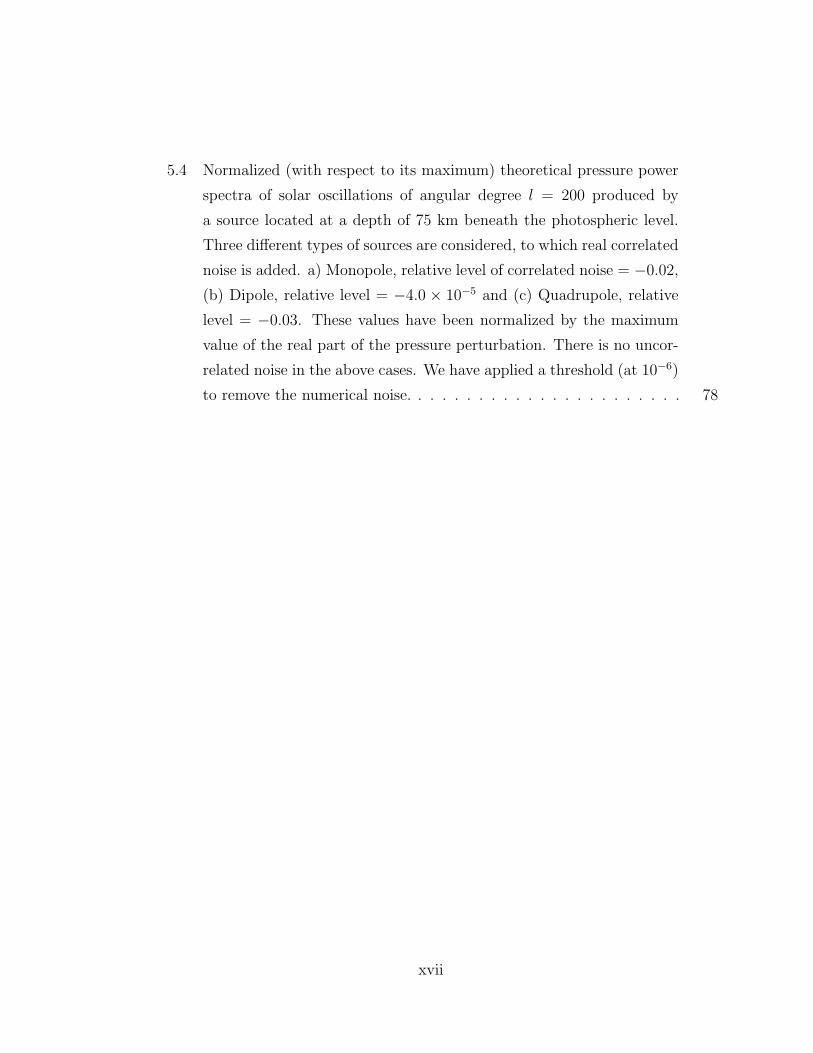
5.4 Normalized (with respect to its maximum) theoretical pressure power
spectra of solar oscillations of angular degree l = 200 produced by
a source located at a depth of 75 km beneath the photospheric level.
Three different types of sources are considered, to which real correlated
noise is added. a) Monopole, relative level of correlated noise = −0.02,
(b) Dipole, relative level = −4.0 × 10⁻⁵ and (c) Quadrupole, relative
level = −0.03. These values have been normalized by the maximum
value of the real part of the pressure perturbation. There is no uncor-
related noise in the above cases. We have applied a threshold (at 10−6)
to remove the numerical noise. . . . . . . . . . . . . . . . . . . . . . . 78
xvii
Chapter 1
Introduction
Solar oscillations have been used to study the structure and rotation of the Sun.
They were first observed by Leighton (1960) to have a period of about five minutes.
A theoretical explanation of their existence was given ten years later by Ulrich (1970)
and, Leibacher and Stein (1971). They described them as standing waves trapped
inside the Sun. About five years later Deubner (1975) observed that the power in
these oscillations as a function of frequency and horizontal wavenumber lies along
ridges. With the discovery of these oscillations the field of helioseismology was born
and since then has blossomed into an exciting new field of astrophysics.
The 1995 launch of the Solar and Heliospheric Observatory (SOHO space mission)
provided near continuous observations free from atmospheric turbulence that made
possible the results in this thesis. With the advent of better data that was not
available in the past, several exciting techniques emerged and the Sun is beginning
to share its secrets.
Oscillations are trapped in the Sun. Studying them enables us to infer the struc-
ture and properties of the Sun. Broadly speaking, solar oscillations consist of two
kinds of waves. The acoustic or p modes are waves in which pressure is the restoring
force. The other kind are internal gravity waves, the g modes, in which gravity is the
restoring force. The g modes have not been unambiguously detected so far. A special
case that deserves mention is the fundamental mode, the f mode, which is a surface
gravity wave having no radial nodes.
1
CHAPTER 1. INTRODUCTION 2
In this thesis, we study the observed properties of the oscillation spectra of p
modes. These oscillations are observed as fluctuations in intensity and line-of-sight
velocity. They produce motion of gas particles and cause Doppler shifts of absorption
lines. The pressure fluctuations of these modes are related to the intensity fluctu-
ations. Various parts of the absorption line are formed in different layers of the
atmosphere. Hence, the height of the observations depends on the position in the
absorption line at which measurements are made. In the Michelson Doppler Imager
(MDI) instrument on board the Solar and Heliospheric Observatory (SOHO) the ob-
servations are made 300 km above the photosphere, in the Nickel I 6768 A absorption
line (Scherrer et al., 1995).
In the next chapter an explanation of the line asymmetry puzzle which was first
observed by Duvall et al. (1993) is given. The power spectra of the oscillations
is not symmetrical, but exhibits varying degrees of asymmetry. Numerous people
have studied this phenomenon (Gabriel, 1992, 1993, 1995), (Abrams and Kumar,
1996), (Roxburgh and Vorontsov, 1995), (Rast and Bogdan, 1998), without finding a
solution to the puzzle. Recently Roxburgh and Vorontsov (1997) proposed a solution.
They suggested that there is velocity overshoot of the granulation which reverses the
asymmetry in the velocity power spectrum. However, observations tend to support
the fact that the reversal of asymmetry occurs in intensity rather than the velocity
power spectrum. This work proposes that the reversal is explained by the presence
of correlated noise due to the granulation which happens to be large in the intensity
fluctuations (Nigam et al., 1998). This conclusion is explained in chapter 2 of the
thesis. At frequencies above the acoustic cutoff frequency, waves propagate and are no
longer trapped in the cavity. Due to the presence of correlated noise, a high frequency
shift between the velocity and intensity power spectrum is predicted by the model.
This is supported by MDI observations.
In chapter 3 the phase difference between velocity and intensity helioseismic spec-
tra is discussed. This was first observed by Deubner and Fleck (1989) from ground
based measurements and later by Straus et al. (1998) from the SOHO instrument.
No satisfactory explanation has been provided for the phase jumps in the vicinity of
an eigenfrequency. According to theory the phase is constant and should not jump.

CHAPTER 1. INTRODUCTION 3
This unusual behavior of the phase is explained by the same model that explains the
reversal of asymmetry. It is the interaction of the oscillations with the background
that results in this peculiar phase difference (Nigam and Kosovichev, 1999a).
Chapter 4 deals with the derivation of an asymmetrical fitting formula using a
simple potential well model (Nigam and Kosovichev, 1998). It takes into account the
correlated noise that is responsible for the reversal in asymmetry. This formula is used
to determine the eigenfrequencies of the p modes, which can then be used to study the
solar structure and rotation. In the past, eigenfrequencies were generally determined
by fitting a symmetrical Lorentzian profile to the asymmetric power spectra. Clearly,
this resulted in errors, as is demonstrated in the chapter. The formula is tested on
low degree p modes and is found to perform quite well (Toutain et al., 1998).
All this leads to the natural question as to how p modes are excited. This is dealt
with in chapter 5. The results in chapters 2 and 3 combine in a self consistent manner
to answer this question. We apply Lighthill’s formulation (Lighthill, 1952), (Stein,
1967), (Goldreich and Kumar, 1988), (Kumar, 1994) and decompose the source into
monopole, dipole and quadrupole types. A very simple model of turbulence is assumed
with regards to the mathematical framework. We find that a model based on a simple
representation of turbulent convection is consistent with the observations suggesting
that the source of oscillations may be turbulent convection. The oscillations appear to
be excited in the superadiabatic layer 75 km below the photosphere by a combination
of monopole and quadrupole sources (Nigam and Kosovichev, 1999b). The monopole
source results from the mass or entropy fluctuations while the quadrupole results from
the Reynolds stresses. The monopole source is the dominant one. The dipole source
as a result of the Reynolds stress forces is ruled out by the observations.
Finally, chapter 6 concludes the thesis pointing to future directions of research,
which follow as extensions of the work presented here.
The thesis uses numerical models to represent the Sun. Studies are made by
comparing the computations from these models with the observed quantities. By
doing this a better insight into the physical processes that work in the Sun can be
gained. I briefly explain below the main observational and theoretical techniques used
in this thesis.
CHAPTER 1. INTRODUCTION 4
1.1 Observations
The observables derived by the MDI instrument that are used here are the Doppler
velocity, line depth and the continuum intensity. It will be worth describing briefly
how this is accomplished. MDI records filtergrams which are images of the solar
photosphere in selectable, well-defined narrow wavelength bands. The observables
are computed by the instrument since there is insufficient telemetry to transmit the
number of filtergrams required to compute these observables at a given cadence and
resolution. Due to this fact, the actual observables are derived quantities based on
multiple sets of filtergrams at five fixed wavelengths separated by 75 mA, denoted by
F0 through F4. F0 being nearly continuum, F1 and F4 centered on the wings and F2
and F3 centered about the core of the center-of-disk Ni I 6768 A line (Scherrer et al.,
1995). The filtergrams are combined onboard by an image processor to produce the
velocity, intensity and line depth measurements which are shown in Figure 1.1, and
are discussed below.
A flexible observing parameter is the resolution. Some studies have been done
with integrated light spectrum over the entire disk (low resolution), and some other
cases have been more successfully done with an imaged (high resolution) map of the
Sun. The issue of resolution depends on the practical objective for a given set of
observations.
1.1.1 Doppler velocity
Velocity measurements usually consist of sampling the intensity of the desired spectral
absorption line at a slightly redshifted and an equally blueshifted wavelength. These
values may then be converted to Doppler wavelength shift using some measure of the
difference between intensities. In other words, the Doppler measurement relates to
a differential measurement in a Fraunhofer line. Since the solar spectrum lines are
rather narrow, typically even a small redshift will give a large intensity difference. This
causes the Doppler measurements to be extremely sensitive. Doppler measurements
are fairly stable, but the effects of solar rotation are significant and care must be
taken to extract them. The velocity imposed by solar rotation is on the order of 2
CHAPTER 1. INTRODUCTION 5
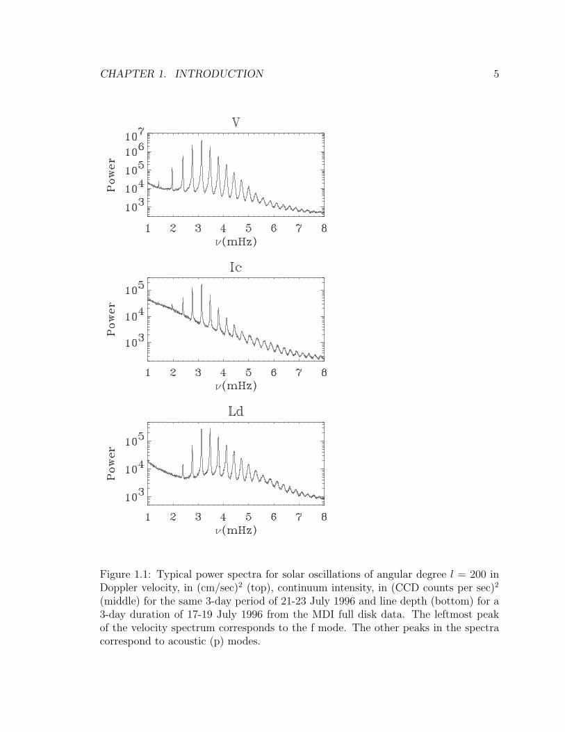
Figure 1.1: Typical power spectra for solar oscillations of angular degree l = 200 inDoppler velocity, in (cm/sec)2 (top), continuum intensity, in (CCD counts per sec)2
(middle) for the same 3-day period of 21-23 July 1996 and line depth (bottom) for a3-day duration of 17-19 July 1996 from the MDI full disk data. The leftmost peakof the velocity spectrum corresponds to the f mode. The other peaks in the spectracorrespond to acoustic (p) modes.
CHAPTER 1. INTRODUCTION 6
km/sec, while the p mode oscillations have a typical velocity of about 50 cm/sec per
mode.
MDI derives an estimate of the Doppler velocity from a ratio of differences of
filtergrams F1 through F4:
α> = [(F1 + F2)− (F3 + F4)]/(F1 − F3) (1.1)
α< = [(F1 + F2)− (F3 + F4)]/(F4 − F2) (1.2)
where the first ratio, equation (1.1), is used with a positive numerator while the latter
equation (1.2) is used to calculate the Doppler velocity when the numerator is less
than or equal to zero. The Doppler shift is calculated from a tabulated nearly linear
function of the filtergram difference ratios. This measurement has several noteworthy
properties:
1) It is essentially blue wing minus red wing intensity divided by continuum minus
line center intensity so it is quite insensitive to variations in the slopes of the wing
intensities. The purpose of this measurement is to get a proxy measure that is nearly
linear over a large dynamic range. The line core actually crosses F2/F3 near the limbs
(Scherrer et al., 1995).
2) It is independent of linear gain and offset variations in the intensity measurements.
1.1.2 Line depth
The line depth proxy is the continuum minus line center intensity. It is estimated
from the four filtergrams by:
Idepth =[2[(F1 − F3)
2 + (F2 − F4)2]
]1/2(1.3)
The formula has similarities to the Doppler calculation since it involves subtracting
filtergrams. Any brightness offsets in the filtergrams due to granulation tend to cancel
in the line depth and Doppler measurements. Therefore there are similarities between
velocity and line depth power spectra (see Figure 1.1).

CHAPTER 1. INTRODUCTION 7
1.1.3 Continuum intensity
Intensity measurements have the advantage of being perhaps one of the easiest mea-
surements to take. No fancy calibrations are required. Intensity measurements are
also less likely to need correction for rotation of the Earth/Sun. However, the fluc-
tuation in intensity due to small oscillations is only on the order of 1 ppm (part-
per-million), so the measurement is very sensitive to any kind of signal degradation.
That is why these measurements are so sensitive to granulation, atmospheric turbu-
lence and cloud interference from the Earth’s surface. Many of these problems are
alleviated with spaceborne observations.
The MDI proxy for the continuum intensity near the Ni-I absorption line of the
measurements is computed with all five filtergrams according to the equation:
Icont = 2F0 + Iave + Idepth/2 (1.4)
where Iave is the average of the four filtergrams, F1 through F4. This formula is
different from the previous two measurements in that there is the (2F0 + Iave) term
which contains the sum of the filtergrams. Any brightness offset due to granulation
in the filtergrams doesn’t cancel in the intensity measurement.
1.1.4 Integrated light techniques
Integrated light techniques used by MDI, which sums CCD pixels have been deployed
previously by the IRIS (International Research on the Interior of the Sun, adminis-
tered by the Universite de Nice, France) instrument (Fossat, 1991). Instruments in
this category use integrated sunlight and so they measure the average surface velocity
over the solar disk. They view the Sun as a star and study p modes of very low degree
(l = 0,1,2). These techniques are unable to study higher degree modes because higher
l modes have nearly equal areas of the disk which are receding and approaching ef-
fectively canceling out any velocity signal when averaged over the entire disk. Since
there is no spatial resolution with this technique, there is no way of isolating out
which mode is being measured.
CHAPTER 1. INTRODUCTION 8
1.1.5 Imaging techniques
The imaging techniques take advantage of modern CCD detectors to record velocity
(or intensity) measurements on a discrete grid over the visible disk. These techniques
have been used by the MDI instrument (Scherrer et al., 1995), where the CCD is a
10242 grid. This method returns a slew more data and allows resolution of individual
modes and analysis of their surface patterns. Usually for imaged methods, a Doppler
measurement is used for its superior signal/noise ratio.
1.2 Data processing
The various steps involved are recording the oscillation (using either intensity or
Doppler velocity measurements), calibrating and correcting the data, splitting the
recorded oscillations into their component spherical harmonics and then analyzing
the resonant frequencies of each individual harmonic.
Step 1: Record the data using either velocity or intensity, which are computed
from the filtergrams.
Step 2: Calibrate all the data. Correct the data for known effects like instrument
drifting, solar rotation, etc. Remove from the velocity a model of the spacecraft mo-
tion and solar rotation.
Step 3: Isolate the contribution from each spherical harmonic. This involves mul-
tiplying the data set at a particular time by one of the spherical harmonics functions
(Y ml , where l is the angular degree and m is the azimuthal order) and integrating over
the disk (Christensen-Dalsgaard, 1994). The resultant is the contribution from that
spherical harmonic degree to the velocity/intensity distribution over the disk. Since
one observes less than half of the Sun, the spherical harmonic functions are no longer
orthogonal, and the modes we isolate are not exactly what we intend to, but a slight
mixture of neighboring modes as well. As a result of this, leakage has to be taken

CHAPTER 1. INTRODUCTION 9
into account. The result from this step is a series of coefficients: one for each har-
monic considered at each time step. The time series are then detrended and gap filled.
Step 4: Convert the time series to frequency (power) spectrum. This is a Fourier
transform (Bracewell, 1986) of each mode in time. The result is a spectrum showing
the frequency content of each mode.
In general, a power spectrum is plotted only for each degree, l. This is because the
modes with different m but same l are almost identical. The m modes cause small
peak splittings, which is used in the analysis of internal rotation rates. There is also
a radial order, n, which we have not taken into account yet, since it is not visible
from the surface. Each peak in the power spectrum corresponds to a different radial
order n for the same degree, l.
The best possible frequency resolution is inversely proportional to observing time
and lifetime, therefore observations should be made for as long as time permits.
This is important for two reasons: firstly, since g modes have long periods and low
amplitudes, and in order to get a strong spectrum, long observation times are required.
A second reason is that Fourier analysis assumes an infinite time series, and discrete
ends to that produce undesirable effects. Data must be recorded often in order to get
a good sampling of the oscillations. This reduces aliasing problems. From the above
discussion it is clear that observations must be recorded for as long and continuous
a period as is possible. Several strategies have been used to achieve the above task.
Observations from the South pole have been carried out in the past, where the Sun
is visible for longer periods of time. Another solution is a network of observing sites
around the globe spaced so that their observing times overlap each other to produce
one continuous data set. A third method that is being tried is to observe from space,
unobstructed by atmospheric effects.
CHAPTER 1. INTRODUCTION 10
1.3 Mode physics
The Sun’s surface is found to be in a state of continuous motion when measured by
the different instruments. There are flares and other bizarre phenomena happening
on the surface. However, measurements of either the velocity or intensity across the
solar disk shows that it is oscillating in a periodic way.
These oscillations, although very complex, are actually combinations of millions
of resonant modes of vibration. Each mode is vibrating at a specific frequency caused
by waves of that frequency resonating in different cavities in the Sun. These cavities
are not gaps and walls in the Sun, like those found in buildings. But rather they are
defined by a combination of both the solar interior properties and the wave frequency.
Only inside a particular cavity are the conditions right for a certain wave to propagate
stably; outside the boundaries, it either is reflected back or decays exponentially.
Solar p modes are sound waves trapped in the cavity. As sound waves propa-
gate into the Sun their sound speed increases due to an increase of temperature.
This causes them to refract continually until they are reflected back to the surface
of the Sun (Christensen-Dalsgaard, 1994). At the surface the solar properties change
abruptly, and waves whose wavelength is smaller than the density scale height prop-
agate, while others get reflected and are trapped in the cavity.
Because the amplitude of the oscillations observed are small compared to their
wavelength, their properties can be studied by means of a linear theory. Therefore,
the oscillations can be decomposed into a linear combination of many resonant modes.
The frequencies of these modes are in turn related to the structure of the interior of the
Sun, and may be calculated using physics of stellar interiors (Christensen-Dalsgaard,
1994).
The mathematical framework used to study these oscillations are the usual equa-
tions of hydrodynamics. Even though we know that this is not true, to simplify
matters we assume a non-rotating, non-magnetic and spherically symmetric Sun.
The equation of continuity which expresses the conservation of mass becomes
∂ρ
∂t+∇ · (ρv) = 0 (1.5)

CHAPTER 1. INTRODUCTION 11
where ρ is the density, t the time and v the velocity.
The equation of motion (Newton’s second law) is
ρ
(∂v
∂t+ v · ∇v
)= −∇p + ρfb (1.6)
where p is the pressure, fb the body forces. Among the possible body forces we
consider only gravity g.
If the motion occurs adiabatically then p and ρ are related by
Dp
Dt= c2
(Dρ
Dt
)(1.7)
where c2 = γ1p/ρ is the sound speed, γ1 is the adiabatic exponent and D/Dt is the
material derivative, following the motion of the fluid element; given by
D
Dt=
∂
∂t+ v · ∇ (1.8)
This is contrasted with the local derivative ∂/∂t at a fixed point. The first three
equations (1.5)-(1.7) form the complete set of equations for adiabatic motion.
The observed solar oscillations have very small amplitudes (maximum velocity of
a superposition of millions of p modes at the surface is about 500 m/sec) compared
with the characteristic scales of the Sun, therefore they can be treated as small pertur-
bations around an equilibrium state. We also assume that the equilibrium structure
is static compared to the oscillation time scale (p modes have a period of about 5
minutes) and that there are no velocities.
Thus by representing each field variable f(r, t) = f0(r)+f ′(r, t), where f0(r) is the
equilibrium state and f ′(r, t) is a small Eulerian perturbation, that is the perturbation
at a given point r, we linearize the above equations about the equilibrium state by
expanding them in the perturbations and retaining only terms that do not contain
products of the perturbations.
The equations (1.5)-(1.6) of continuity and motion become
∂ρ′
∂t+∇ · (ρ0v
′) = M(r, t) (1.9)

CHAPTER 1. INTRODUCTION 12
ρ0∂v′
∂t+∇p′ + ρ′g0 = F (r, t) (1.10)
The right hand sides of the equations are the source terms which drive the os-
cillations. In deriving the above equations the Cowling approximation was applied,
with the neglect in the perturbation of the acceleration due to gravity (Christensen-
Dalsgaard, 1994). Here M and F are the mass and force sources and are given by:
M = −∇ · (ρ′v′) (1.11)
F = −ρ′∂v′
∂t−∇ · (ρ0v
′v′) (1.12)
It is convenient to transform the above equations expressing the Eulerian pertur-
bations in terms of the Lagrangian perturbations, which are perturbations following
the motion of the fluid. They are related as
δf(r) = f ′(r0) + δr · ∇p0 (1.13)
where δf is the Lagrangian perturbation of the field variable f and δr is the fluid
displacement. The velocity v is given by the time derivative of the displacement δr
The equation for adiabatic motion becomes
δp = c20δρ (1.14)
where c0 is the equilibrium sound speed, which is computed from a solar model.
The fluid displacement can be written in terms of the spherical harmonics Y ml (θ, φ)
δr = 2√
πRe
[(ψr(r), ψh(r)
∂
∂θ,ψh(r)
sin θ
∂
∂φ
)Y m
l (θ, φ) exp(iωnlt)
](1.15)
where r is the distance from the center, θ is the colatitude (angle from the polar
axis), φ is the longitude and ψr and ψh are the radial and horizontal components of
the displacement. The angular frequency ωnl is complex and contains the effect of
CHAPTER 1. INTRODUCTION 13
the damping. In this thesis viscous damping is considered.
Carrying out the spherical harmonic decomposition of the equations of mass and
momentum leads to the following ordinary differential equations, with the subscripts
nl dropped in the angular frequency ω and the subscript 0 dropped from the equilib-
rium variables:dψr
dr+ ψr
(2
r+
d ln ρ
dr
)+
ρ′
ρ− l(l + 1)
ρr2ω2p′ = S1 (1.16)
dp′
dr+ gρ′ − ω2ρψr = S2 (1.17)
The sources S1 and S2 are
S1 =1
ρω2
∫dt exp(−iωt)
∫ dΩ
ρFh (1.18)
S2 = −∫
dt exp(−iωt)∫
dΩ Fv (1.19)
where Ω is the solid angle, Fh and Fv contain the horizontal and radial component of
the forces and are given by:
Fh =
[1
r
∂Y m∗l
∂θFθ +
1
r sin θ
(∂Y m∗
l
∂φ
)Fφ − ∂2M
∂t2
](1.20)
Fv = Y m∗l Fr (1.21)
where F = (Fr, Fθ, Fφ) and * is the complex conjugate.
The above equations (1.16) and (1.17) can be rewritten involving Lagrangian
perturbations (Gough, 1993) and become:
dξ
dr+
(2
r− L2g
ω2r2
)ξ +
(1− L2c2
ω2r2
)δp
ρc2= S1 (1.22)
dδp
dr+
L2g
ω2r2δp− gρf
rξ = S2 (1.23)
where L2 = l(l + 1), ξ = ψr and the discriminant f is

CHAPTER 1. INTRODUCTION 14
f = 2 +ω2r
g+
r
Hg
− L2g
ω2r(1.24)
where H−1g is the scale height of the gravitational acceleration and is
H−1g = −d ln g
dr(1.25)
By differentiating equation (1.23) with respect to r and using equation (1.22) to
eliminate dξdr
and then using equation (1.23) to eliminate ξ, an equation for δp is
obtained:
d2δp
dr2+ H−1
u
dδp
dr+
[1
c2
(ω2 +
g
h
)− L2
r2
(1− N2
s
ω2
)]δp = S12 (1.26)
where H−1u and Ns are
H−1u = H−1 + H−1
f + H−1g + 3r−1 (1.27)
N2s = g
(H−1
u − g
c2− 2h−1
)(1.28)
and h−1 = H−1g + 2r−1 is the scale height of g
r2 and H−1f is the scale height of f .
It is convenient to reduce equation (1.26) into more compact form by means of
the transformation (Gough, 1993)
δp =
(gρf
r3
)1/2
Ψ := uΨ (1.29)
d2Ψ
dr2+ K2Ψ = S (1.30)
where S = S12/u, is given by
S(r, ω) =
[c1
dS2
dr+ c2S2
]+
[c3
dS1
dr+ c4S1
], (1.31)
where c1, c2, c3 and c4 depend on the solar model and are given in Appendix A.1 and
K is

CHAPTER 1. INTRODUCTION 15
K2 =ω2 − ω2
cs
c2+
l(l + 1)
r2
(N2
s
ω2− 1
)(1.32)
where ωcs is
ω2cs =
c2
4H2u
(1− 2
dHu
dr
)− g
h(1.33)
Here H−1u is the scale height of the factor u defined in equation (1.29). Medium l
oscillations are confined to the outer convective layers of the Sun, hence the effect of
spherical geometry can be neglected. In the plane-parallel approximation ωcs reduces
to ωc the acoustic cutoff frequency and Ns reduces to N the buoyancy frequency,
which are given below:
ω2c =
c2
4H2
(1− 2
dH
dr
)(1.34)
N2 = g(
1
H− g
c2
)(1.35)
where H−1 is the density scale height:
H−1 = −d ln ρ
dr(1.36)
The solutions to this reduced wave equation (1.30) are evanescent if K2 < 0, and
waves propagate when K2 > 0. The two frequencies define the cavities in the Sun.
It follows from the constraint K2 > 0 that there are two different types of cavities,
where the p and g modes propagate. This can be easily seen if we rewrite K as:
K2 =ω2
c2
(1− ω2
+
ω2
) (1− ω2
−ω2
)(1.37)
This makes it clear that there are two separate propagation zones: where the wave
frequency ω > ω+, and where ω < ω−. These boundary frequencies ω+ and ω− are
given by
ω2+ =
1
2(S2
l + ω2cs) +
[1
4(S2
l + ω2cs)
2 −N2s S2
l
]1/2
(1.38)

CHAPTER 1. INTRODUCTION 16
ω2− =
1
2(S2
l + ω2cs)−
[1
4(S2
l + ω2cs)
2 −N2s S2
l
]1/2
(1.39)
where Sl is the Lamb frequency and is
S2l =
c2L2
r2(1.40)
In the interior of the Sun, the equations (1.38) and (1.39) can be approximated
by:
ω2+ ≈
c2l(l + 1)
r2(1.41)
ω2− ≈ N2 (1.42)
Waves that propagate in the region defined by ω > ω+ are called p modes, and
those that resonate in the ω < ω− region are called g modes. Waves with frequency
in the range ω− < ω < ω+ are evanescent. A plot of the solar potential ν+ and ν− is
shown in Figure 1.2
1.3.1 P modes
P modes are standing pressure waves trapped in the Sun. They propagate stably in
the region of the Sun defined by ω > ω+.
For p modes,
K2 ≈ ω2 − ω2+
c2(1.43)
The upper limit of this region is essentially when the wave frequency equals the
acoustic cutoff frequency, and depends only on the speed of sound c and the density
scale height H. For p modes the discriminant f > 0 in equation (1.24) (Gough, 1993).
Once a wave reaches the point where its frequency equals this cutoff frequency, it
is sharply reflected back inward. This cutoff point is fairly constant, between about
0.98 and 0.99 solar radii. However, it does have a finite upper limit in the outer layers
CHAPTER 1. INTRODUCTION 17
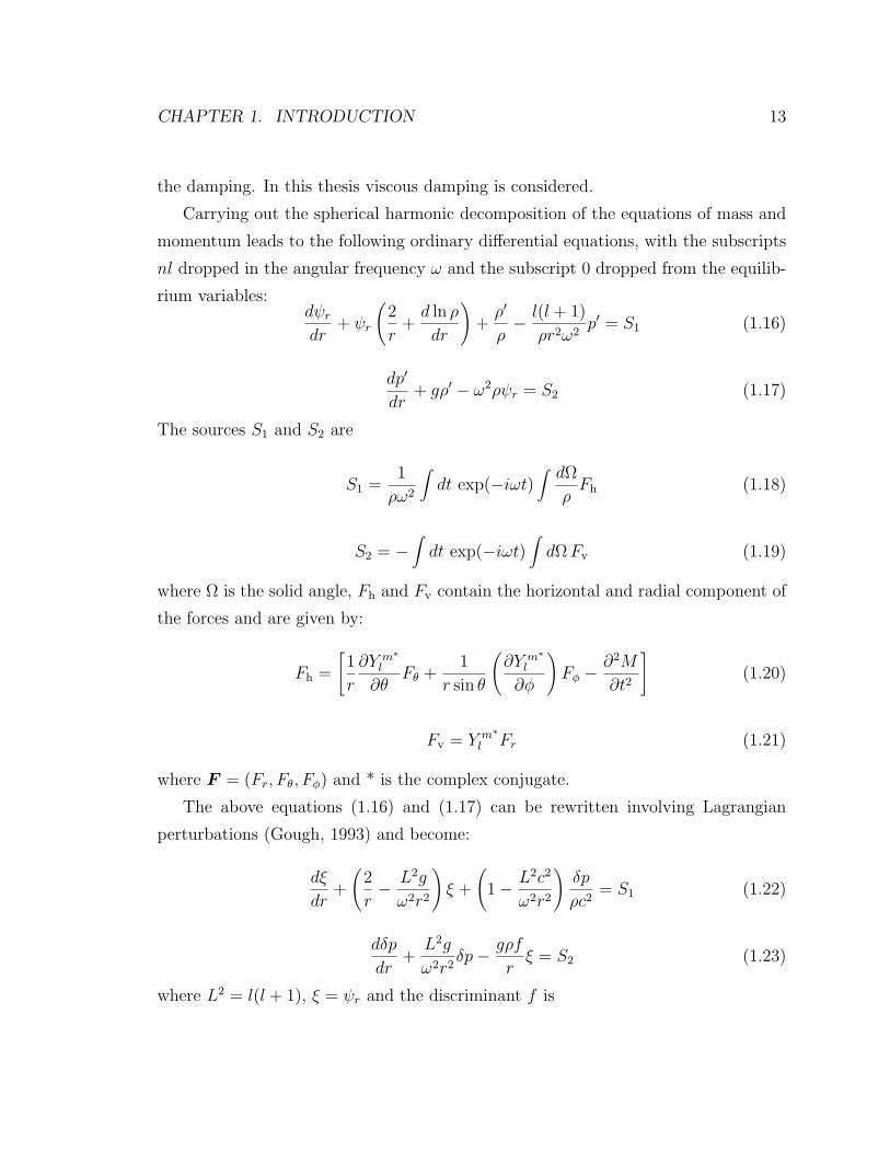
Figure 1.2: Solar potentials ν+ = ω+/2π and ν− = ω−/2π as a function of depth h forfor angular degree l = 1000. Depth 0 indicates the photosphere and negative depthsare below the photosphere.
of the Sun. If a wave has a frequency greater than ωc then it will not be reflected
back into the Sun. This constrains the p modes to have resonant frequencies lower
than a specific value, set by the stellar structure.
The inner boundary of the p mode propagation cavity is caused by an increase
in sound speed, c, towards the center of the Sun due to increase in temperature. As
c increases, the inner edge of the wave (closer to the core of the Sun) moves faster
than the outer edge, causing the wave to gradually refract towards the surface. As
the wave propagates deeper into the Sun, the wave is continually refracted until it is
completely reflected. This inner turning point is described by the Lamb frequency Sl.
High frequency p modes include waves with ω > ωc, νc = ωc/2π = 5.2 mHz. These
waves propagate and are not trapped by the photosphere. It was therefore a surprise
to find p mode ridges continue above the acoustic cutoff. The explanation by Kumar
and Lu (1991) states that waves are emitted isotropically from a source near the top
CHAPTER 1. INTRODUCTION 18
of the convection zone. Waves that propagate directly from the source interfere with
the waves that are reflected from below due to the continual increase in sound speed.
This interference is responsible for the observed high frequency ridges and this is true
for the ridges above l = 200 as well. These high frequency waves suffer some amount
of reflection in the solar atmosphere.
Note that this inner turning point does depend on the mode degree. For higher
degree modes, the turning point will be nearer to the surface than for low degree
modes. This is important, because it tells us how far a mode of particular degree
penetrates into the interior of the Sun. Low order, low degree waves penetrate the
deepest of all the modes. High degree (l > 60) don’t penetrate any deeper than the
convective layer, whereas low degree modes travel deeper down up to about 0.05 solar
radii. Radial modes (l = 0) propagate right through the core (Christensen-Dalsgaard,
1994). The lower and upper turning points are shown in the plot of the solar acoustic
potential ν+ = ω+/2π in Figure 1.2.
1.3.2 G modes
G modes are rather mysterious. They hide deep within the solar interior and have
not yet been observed. The main restoring force for these modes is buoyancy. The
waves are essentially oscillations of packets of gas moving around their hydrostatic
equilibrium position. If some initial disturbance perturbs the gas from equilibrium,
it may rise above the equilibrium position only to find that its density is then greater
than the new surroundings. The gas then sinks back down, but overshoots the equi-
librium position, until it is in a region where its density is less than the surrounding
gas. The packet is then forced up, and so on... The frequency of these waves is the
buoyancy frequency.
G modes, like the p modes, are trapped within a cavity in the solar interior. These
waves oscillate in a region defined by ω < ω−. The upper limit of this region is the
bottom of the convective layer, since in the convection zone the gravity waves are no
longer stable.
The inner limit of the g mode cavity is defined by the buoyancy frequency N . The
CHAPTER 1. INTRODUCTION 19
lower turning point occurs when ω = ω−, or in other words when the wave frequency
equals the buoyancy frequency. In the stable g mode region, ω− is less than N . But
as the wave travels towards the center, the gravitational acceleration reduces to the
point till N = ω−. This is the turning point. Therefore g modes are nothing but
standing internal gravity waves. For g modes f < 0 (Gough, 1993).
Gravity modes can be trapped either beneath the convection zone or in the atmo-
sphere (Christensen-Dalsgaard, 1994). A single mode can exist in both regions; how-
ever, the evanescent decay is so great through the turbulent convection that extremely
weak coupling between the atmosphere and the interior is likely to be destroyed by
turbulence. Thus for practical purposes the interior modes and the atmospheric
modes can be regarded as distinct.
G modes have much longer periods than the p modes (Christensen-Dalsgaard,
1994). Typical g mode periods are of the order of 165 minutes. Many observations
have been done to detect these modes, but because of their very long periods and
low amplitudes (as they are localized around the core of the Sun), the data and
interpretations are full of ambiguities.
1.3.3 F mode
The p and g modes are separated by a mode with no radial node, whose frequency lies
between those of the p and g modes. This mode can exist only when l 6= 0. Cowling
called it the f mode, for fundamental gravity mode (Christensen-Dalsgaard, 1994).
The f mode is a special type of the g mode. It is the surface gravity wave that
exists at the interface of fluids of differing density. The f mode propagates without
compression, so it produces no pressure fluctuations. It has been observed in both
the velocity and intensity observations, but not in line depth. The reason why it is
present in intensity is not well understood. Since the f mode is a surface gravity wave,
it has proved useful to study the surface magnetic fields, the constraining of the solar
radius and other interesting surface effects. Moreover the frequencies of the f mode
depend only on their wavelength and on gravity, but not on the internal structure of
the layer, in particular the density. Its dispersion relation is given by ω2 = gk, where

CHAPTER 1. INTRODUCTION 20
g is the acceleration due to gravity computed from the solar model and k = L/RSun is
the wave number and RSun is the solar radius. The f mode satisfies the discriminant
f = 0 (Gough, 1993). The displacement eigenfunction decays exponentially with
depth from the solar surface, which is an indication that the mode is concentrated
in the uppermost layers of the Sun, particularly when k is large. Since the f mode
propagates horizontally, it can be used to study supergranules and horizontal flow
fields.
So, the Sun is observed to resonate at certain harmonic frequencies. Which fre-
quencies are resonant is a combination of the frequency of the wave and the size of
the cavity it is trapped in. Waves of millions of frequencies are excited in the inte-
rior of the Sun, but the specific structure of the Sun selects which exact frequencies
are resonant. These frequencies are a measure of the interior structure of the Sun.
Studying the p, g and f modes together would be useful in solving the mysteries of
the Sun.
Before proceeding to discuss the excitation and damping of p modes, it will be
worthwhile to review Lighthill’s theory of sound generation.
1.4 Lighthill’s theory
Sir James Lighthill in 1952 propounded his theory of sound generation due to fluid
flow, with rigid boundaries. According to his theory sound is generated by a conver-
sion of kinetic enery into acoustic, as a result of fluctuations in the flow of momentum
across fixed surfaces.
The propagation of sound in a uniform medium, without sources of matter or
external forces is governed by the equation of continuity and linearized equation of
momentum
∂ρ
∂t+
∂
∂xi
(ρvi) = 0, (1.44)
∂
∂t(ρvi) + c2
0
∂ρ
∂xi
= 0 (1.45)

CHAPTER 1. INTRODUCTION 21
Eliminating the momentum density ρvi from equations (1.44) and (1.45) leads to
∂2ρ
∂t2− c2
0∇2ρ = 0 (1.46)
Here ρ is the density, vi is the velocity in the xi direction and c0 is the sound speed
in the uniform medium.
On the other hand, the original equation of momentum in an arbitrary continuous
medium under no external forces in Reynolds’s form is
∂
∂t(ρvi) +
∂
∂xj
(ρvivj + pij) = 0 (1.47)
Here pij is the compressive stress tensor, representing the force in the xi direction
acting on a portion of fluid, per unit surface area with inward normal in the xj
direction. The other term ρvivj is the momentum flux tensor, that is the rate at
which momentum in the xi direction crosses unit surface area in the xj direction.
This equation can be obtained from the momentum equation in the familiar Eulerian
form by adding a multiple of the equation of continuity, equation (1.44). Physically,
this equation represents the fact that the momentum contained within a fixed region
of space as changing at a rate equal to the combined effect of (i) the stresses acting
at the boundary pij and (ii) the flow across the boundary of momentum-bearing fluid
due to ρvivj.
Hence the equations of an arbitrary fluid motion can be rewritten as the equa-
tions of propagation of sound in a uniform medium at rest due to externally applied
fluctuating stresses, namely, as
∂
∂t(ρvi) + c2
0
∂ρ
∂xi
= −∂Tij
∂xj
(1.48)
∂2ρ
∂t2− c2
0∇2ρ =∂2Tij
∂xi∂xj
(1.49)
where the instantaneous applied stress at any point is
Tij = ρvivj + pij − c20ρδij (1.50)

CHAPTER 1. INTRODUCTION 22
Equations (1.48) and (1.49) are the basic equations of the theory of aerodynamic
sound generation (Lighthill, 1952).
It has been pointed out in Lighthill’s paper that all effects such as the convection
of sound by the turbulent flow, or the variations in the sound speed within it, are
taken into account, by incorporation as equivalent applied stresses, in equations (1.48)
and (1.49). Thus outside the airflow the density satisfies the ordinary equations of
sound, with out the stress Tij in equations (1.45) and (1.46), and the fluctuations
in density, caused by the effective applied stresses within the airflow, are propagated
acoustically. These stresses are responsible for the quadrupolar emission of sound.
The theory of sound generated aerodynamically was extended by Lighthill (1953),
to take into account the statistical properties of turbulent airflows, from which the
sound radiated (without the help of solid boundaries) is called aerodynamic noise. The
quadrupole distribution is shown to behave as if it were concentrated into independent
quadrupoles, one in each average eddy volume.
1.5 Excitation and damping of p modes
P modes have a period of about 5 minutes and are believed to be excited as a result
of granulation in the outer turbulent convective zone (Goldreich and Keeley, 1977).
The granulation turnover time is roughly 5 minutes, which suggests that p modes
are excited as a result of granulation. The maximum amplitude of a superposition
of velocity oscillations is small compared to the other characteristic scales of the
Sun, and is about 500 m/sec. The convective currents randomly excite different
frequencies within the Sun. Any given resonant oscillation gets damped and dies out
after a lifetime of anywhere from hours to years, then is reexcited at some later time
by the same random motion of the convective currents.
The linearized hydrodynamic equations derived in the previous sections ade-
quately describe the excitation of p modes. The right hand side of the continuity
equation (1.9) contains the mass term (monopole source), the momentum equation
(1.10) has a force term (dipole source) on the right hand side. The force term contains
the turbulent Reynolds stress, which is responsible for the quadrupole source. These
CHAPTER 1. INTRODUCTION 23
sources could be produced by fluctuations in entropy. The physical significance of
each of these sources along with their role in p mode excitation is discussed in the
following subsections.
1.5.1 Monopole source
The monopole source results by forcing the mass in a fixed region of space to fluctuate
(Crighton, 1975). By this kinetic energy is coverted into acoustic energy. A way of
achieving this in linear acoustics is to suppose that sources of mass are distributed
throughout the fluid, injecting fluid mass at a given rate. The right hand side of the
linearized continuity equation describes the mass source. A time dependent mass flux,
e.g., popping a balloon, cracking a finger, radially pulsating sphere etc. results in a
monopole source. Entropy fluctuations due to radiative cooling at the solar surface
are responsible for the monopole source in the Sun.
1.5.2 Dipole source
The dipole source results by forcing the momentum in a fixed region of space to
fluctuate. This type of source is exactly equivalent to an external force distribution
acting on the fluid (Crighton, 1975). The right hand side of the linearized momentum
equation contains the force, which acts as the dipole source. The monopole and
dipole terms are related in the Sun, since an increase in entropy will cause both an
increase in the volume of the gas (the monopole part) and, because of the gravitational
field, a change in the momentum of the gas (the dipole part). A time-varying force
(momentum flux) is responsible for dipole emission such as sound from a musical
string or a tuning fork or the force due the Reynolds stresses in the Sun.
1.5.3 Quadrupole source
The quadrupole source results by forcing the rates of momentum flux across fixed
surfaces to vary, as when sound is generated aerodynamically with no motion of
solid boundaries. In a theoretical treatment, the real fluid, in which highly-nonlinear

CHAPTER 1. INTRODUCTION 24
motions may occur, is replaced by a fictitious acoustic medium, in which only small
amplitude linear motions occur. If this medium is acted upon by an external stress
system, then exactly the same density fluctuations will be produced. This is the
basis of Lighthill’s theory. The quadrupole stress distribution is derived from dipoles
in exactly the same way as the dipole from a monopole by a limiting process. A
quadrupole is formed by taking the limit of two adjacent equal and opposite dipoles.
Thus, there are two characteristic directions associated with a quadrupole: one the
direction of the individual dipoles, the other the direction in which the dipoles are
separated. Since there are three components of each direction, there are nine possible
independent orientations of the quadrupole axes. These divide into a group of three
longitudinal quadrupoles in which the dipoles or monopoles are arranged in a line and
in which both characteristic directions coincide, and a group of six lateral quadrupoles
with mutually perpendicular characteristic directions (Crighton, 1975). Now, two
equal and opposite adjacent forces constitute a stress; a pressure type stress in the
longitudinal case, a shear stress in the lateral case. Internal stresses with no associated
mass or momentum flux as in the case of free turbulence is responsible for quadrupolar
emission of acoustic waves. In the Sun Reynolds stresses act as quadrupole sources.
For Lighthill’s theory to be valid, the physical conditions should be such that
wave motions, satisfying the homogeneous wave equation, do emerge at sufficiently
great distances from the unsteady flow. Therefore, Lighthill’s theory reduces to the
ordinary acoustic theory at all points outside the region of unsteady flow.
1.6 Why is this problem important?
By studying the excitation of p modes one learns the underlying physics of excitation
and about the source of these modes. This is then useful in deriving a fitting formula
to accurately determine the p mode eigenfrequencies by fitting the observed velocity
and intensity power spectra. An accurate determination of the frequencies will in
turn have an effect on the inversions to determine the solar structure and rotation
rate.

Chapter 2
The Line Asymmetry Puzzle(Part of this chapter is published in ApJ 1998, 495, L115)
Line asymmetry is closely linked to the excitation of p modes. Observations of Duvall
et al. (1993) have indicated that the power spectrum of solar acoustic (p) modes
show varying amounts of asymmetry. In particular, the velocity and intensity power
spectra revealed an opposite sense of asymmetry. There was scepticism about the
result (Abrams and Kumar, 1996), and it was even believed to be an error in the
experiment. However, the new MDI data presented here confirm the result and, in
addition, allow us to study the variations of asymmetry among modes of various
angular degrees and frequencies.
The variations in the asymmetry have important implications in helioseismology
where the eigenfrequencies are generally determined by assuming that the line profile
is symmetric and can be fitted by a Lorentzian. This leads to systematic errors in
the determination of frequencies and, thus, affects the results of inversions.
Several authors have studied this problem theoretically and have found that there
is an inherent asymmetry when the solar oscillations are excited by a localized source
(Gabriel, 1992); (Duvall et al., 1993); (Roxburgh and Vorontsov, 1995); (Abrams
and Kumar, 1996); (Nigam et al., 1997). Physically, the asymmetry is an effect of
interference between an outward direct wave from the source and a corresponding
inward wave that passes through the region of wave propagation (Duvall et al., 1993).
However, the precise cause for the asymmetry and its relation to the Sun’s acoustic
25
CHAPTER 2. THE LINE ASYMMETRY PUZZLE 26
source have not been pinned down in the past. We briefly describe the observations,
formulate a theoretical model and from it suggest an explanation for the difference in
asymmetries between velocity and intensity and finally estimate the depth and type
of the sources that are responsible for exciting the solar p modes.
2.1 Observations
To compare the asymmetry in velocity and intensity spectra we computed spherical
harmonic transforms (SHTs) of full disk velocity and intensity images from the MDI
instrument (Scherrer et al., 1995). These SHT’s were gap filled, Fourier transformed
to make power spectra, shifted in frequency according to a solar rotation law, and
averaged over the angular order m. To simplify the comparison we chose the days
July 21 to July 23, 1996 for which simultaneous velocity and intensity images were
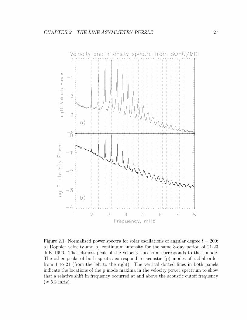
available. The results for oscillations of angular degree l = 200 are shown in Figure
2.1.
From these two power spectra that have been normalized with respect to the
maximum power we see that the p mode peaks of the velocity spectrum have negative
asymmetry (more power on the low frequency end of the peak) while the peaks of
the intensity spectrum have positive asymmetry (more power on the high frequency
end of the peak). In the velocity spectrum (Figure 2.1a), the asymmetry is strongest
for low frequency (low radial order) modes and becomes negligible around and above
the acoustic cutoff frequency (≈ 5.2 mHz). However, the asymmetry in the intensity
oscillations (Figure 2.1b) increases with frequency for modes below the acoustic cutoff
frequency, and then gradually decreases at higher frequencies. The intensity spectrum
shows a higher noise level compared to the velocity spectrum.
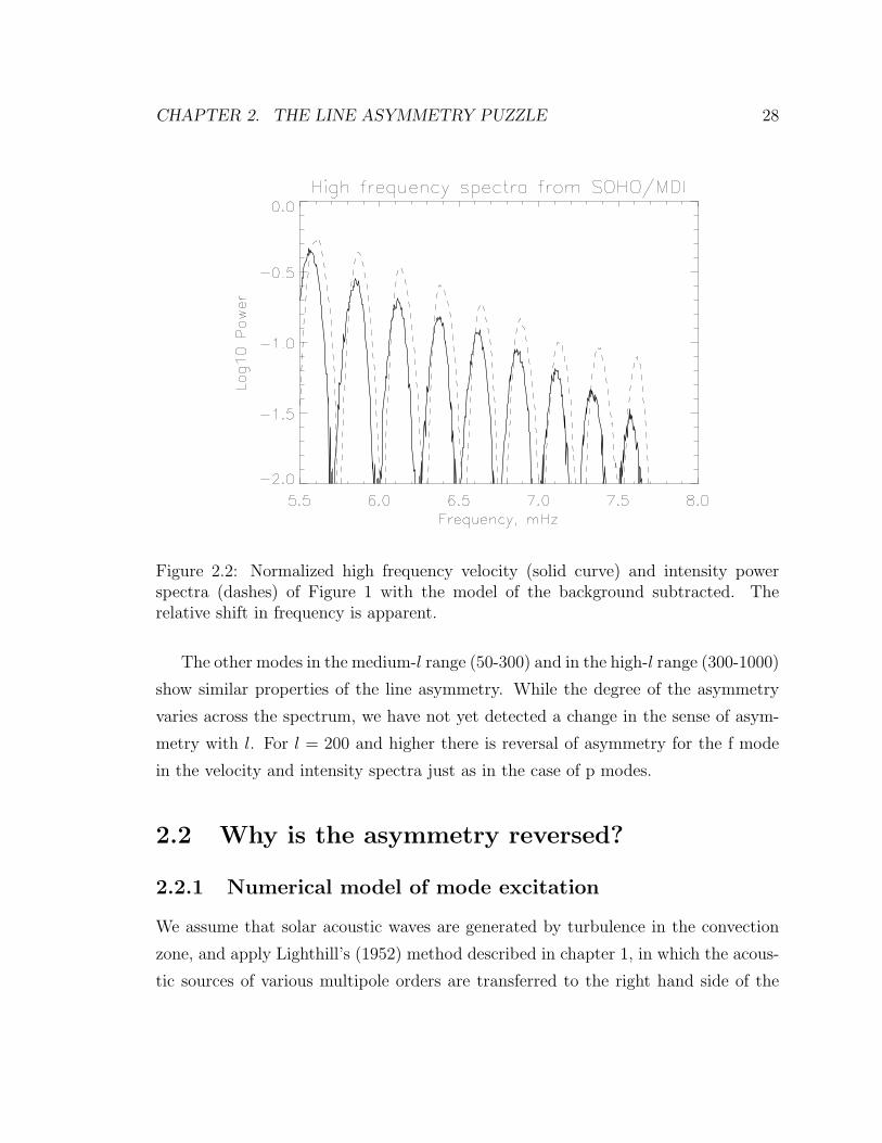
Also in Figure 2.2 with the model of the additive background subtracted a notable
shift in the peaks at the high frequency part of the intensity spectrum is seen in
relation to the same part of the velocity spectrum. This frequency shift is particularly
strong at and above the acoustic cutoff frequency. This is due to the fact that around
the acoustic cutoff frequency, a transition from the dominance of well resonance to
source resonance takes place (see section 2.2.3).
CHAPTER 2. THE LINE ASYMMETRY PUZZLE 27
Figure 2.1: Normalized power spectra for solar oscillations of angular degree l = 200:a) Doppler velocity and b) continuum intensity for the same 3-day period of 21-23July 1996. The leftmost peak of the velocity spectrum corresponds to the f mode.The other peaks of both spectra correspond to acoustic (p) modes of radial orderfrom 1 to 21 (from the left to the right). The vertical dotted lines in both panelsindicate the locations of the p mode maxima in the velocity power spectrum to showthat a relative shift in frequency occurred at and above the acoustic cutoff frequency(≈ 5.2 mHz).
CHAPTER 2. THE LINE ASYMMETRY PUZZLE 28
Figure 2.2: Normalized high frequency velocity (solid curve) and intensity powerspectra (dashes) of Figure 1 with the model of the background subtracted. Therelative shift in frequency is apparent.
The other modes in the medium-l range (50-300) and in the high-l range (300-1000)
show similar properties of the line asymmetry. While the degree of the asymmetry
varies across the spectrum, we have not yet detected a change in the sense of asym-
metry with l. For l = 200 and higher there is reversal of asymmetry for the f mode
in the velocity and intensity spectra just as in the case of p modes.
2.2 Why is the asymmetry reversed?
2.2.1 Numerical model of mode excitation
We assume that solar acoustic waves are generated by turbulence in the convection
zone, and apply Lighthill’s (1952) method described in chapter 1, in which the acous-
tic sources of various multipole orders are transferred to the right hand side of the
CHAPTER 2. THE LINE ASYMMETRY PUZZLE 29
wave equation (Moore and Spiegel, 1964), to calculate the velocity and pressure per-
turbations. We also assume that the observed intensity variations recorded by the
MDI instrument correspond to Lagrangian pressure (or temperature) perturbations
(Duvall et al., 1993); (Abrams and Kumar, 1996).
The background state is assumed to be spherically symmetrical, and all the per-
turbations are time harmonic. Dissipation is modeled by viscous damping. Then,
using a standard decomposition onto spherical harmonics (Gough, 1993); (Gabriel,
1993) we transform Lighthill’s equations of motion, continuity and energy (the full
non-adiabatic problem is at least of the fourth order) into a simplified single second-
order wave equation (see equation (1.30) in chapter 1)
d2Ψ
dr2+
[ω2 − ω2
c
c2− l(l + 1)
r2
(1− N2
ω2
)]Ψ = S[f , q], (2.1)
where Ψ is proportional to the Lagrangian pressure perturbation δp (Gough, 1993), r
is the radius, ω is the frequency, ωc is the acoustic cutoff frequency, c is the equilibrium
sound speed, N is the equilibrium buoyancy frequency, S is a combination of source
terms that include the fluctuating Reynolds stress force, f and the mass source, q.
In this research, we consider a source given in equation (2.2) that is a combination
of monopole (mass source) and dipole (Unno, 1964). The dipole part results when
a monopole source is in a stratified medium and also from the radial and horizontal
components of the Reynolds stress force. The radial component of the force is more
dominant than its horizontal counterpart for data of medium angular degree l. The
expression for S is proportional to the sum of q, f and their respective derivatives with
respect to r. This type of composite source gives a good match with the MDI intensity
and velocity data, and is given by (see chapter 1 equation (1.31) and Appendix A.1,
equation (A.9))
S(r, ω) =
[c1
dS2
dr+ c2S2
]+
[c3
dS1
dr+ c4S1
], (2.2)
where c1, c2, c3 and c4 depend on the solar model. S1 is a source that contains the
mass term and the horizontal component of the Reynolds stress force. S2 contains
CHAPTER 2. THE LINE ASYMMETRY PUZZLE 30
the radial component of the Reynolds stress force. S1 scales as ω−2 while S2 does not
contain ω explicitly as discussed in Kumar (1994).
The Green’s function GΨ(r, rs) of equation (2.1) for a delta-function source at
r = rs using a standard solar model (Christensen-Dalsgaard et al., 1996), is found
numerically using finite differences. The Sommerfeld radiation condition is applied
above the upper turning point to ensure outgoing waves and GΨ(r, rs) = 0 at r = 0
as the perturbations are negligible much below the lower turning point. Damping
is added by making the frequency complex, the imaginary part having the damping
coefficient. Since the source is close to the surface, where dissipative effects vary with
position, the damping coefficient is a function of position. Two kinds of damping,
spatial, similar to Abrams and Kumar (1996), and temporal damping, were inves-
tigated. It is found that they have very little effect on line asymmetry. Damping
basically effects the line width. The resulting system is a complex tridiagonal matrix
equation which is solved by a standard routine (see Appendix A.2 for the numerical
solution). To compare with the observations we multiplied the Green’s function with
a suitable source function and then added noise that was correlated with this source
in a frequency dependent manner.
2.2.2 Effect of correlated noise
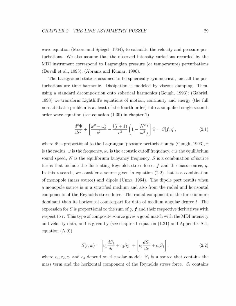
For the solar potential of the simplified model, the real part of the Green’s function
for the pressure perturbation is calculated from equation (2.1) and shown in Figure
2.3. It has been normalized with respect to its maximum value. The corresponding
imaginary part is plotted in Figure 2.4. The intersection of the dashes with the
Green’s function (solid line) in Figure 2.3 correspond to points of zero amplitude,
which result when there is no driving by the source.
The Lagrangian perturbations are then calculated from the Green’s function for
a single source location and source type by multiplying by a suitable source function
and adding solar noise. The noise is assumed to consist of a part cp(ν) that is
correlated with the source function s(ν), while np(ν) forms the uncorrelated additive
background. One then obtains for the pressure perturbation
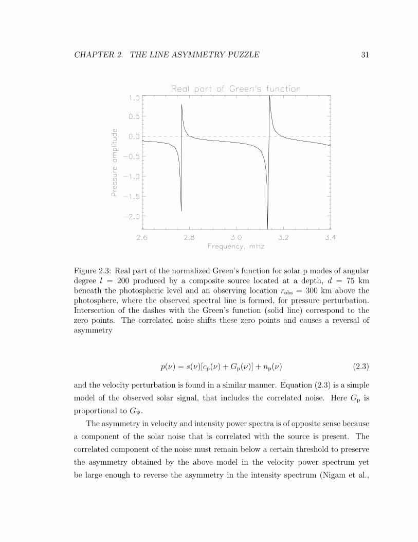
CHAPTER 2. THE LINE ASYMMETRY PUZZLE 31
Figure 2.3: Real part of the normalized Green’s function for solar p modes of angulardegree l = 200 produced by a composite source located at a depth, d = 75 kmbeneath the photospheric level and an observing location robs = 300 km above thephotosphere, where the observed spectral line is formed, for pressure perturbation.Intersection of the dashes with the Green’s function (solid line) correspond to thezero points. The correlated noise shifts these zero points and causes a reversal ofasymmetry
p(ν) = s(ν)[cp(ν) + Gp(ν)] + np(ν) (2.3)
and the velocity perturbation is found in a similar manner. Equation (2.3) is a simple
model of the observed solar signal, that includes the correlated noise. Here Gp is
proportional to GΨ.
The asymmetry in velocity and intensity power spectra is of opposite sense because
a component of the solar noise that is correlated with the source is present. The
correlated component of the noise must remain below a certain threshold to preserve
the asymmetry obtained by the above model in the velocity power spectrum yet
be large enough to reverse the asymmetry in the intensity spectrum (Nigam et al.,

CHAPTER 2. THE LINE ASYMMETRY PUZZLE 32
Figure 2.4: Imaginary part of the normalized Green’s function for solar p modes ofangular degree l = 200 produced by a composite source located at a depth, d = 75km beneath the photospheric level and an observing location robs = 300 km above thephotosphere, where the observed spectral line is formed, for pressure perturbation.
1998). The source position rs from the origin is kept fixed and the power spectrum
is computed from equation (2.3) for the pressure perturbation. It is found that the
correlation cp(ν) reverses the asymmetry found in Gp(ν) when computing the power
spectrum as seen from Figure 2.4b. This is due to the fact that cp shifts the zero
points in Gp(ν). The uncorrelated noise plays no role in the reversal of asymmetry.
The intensity and velocity fluctuations are computed from the absorption line that
is formed at a particular height in the solar atmosphere. The spectral line is effected
by the p mode oscillations and the solar granulation, which modulate and shift the
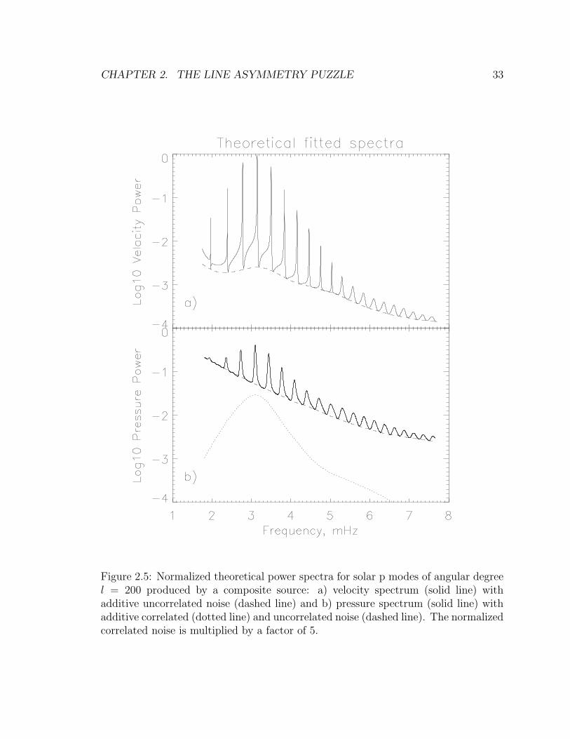
CHAPTER 2. THE LINE ASYMMETRY PUZZLE 33
Figure 2.5: Normalized theoretical power spectra for solar p modes of angular degreel = 200 produced by a composite source: a) velocity spectrum (solid line) withadditive uncorrelated noise (dashed line) and b) pressure spectrum (solid line) withadditive correlated (dotted line) and uncorrelated noise (dashed line). The normalizedcorrelated noise is multiplied by a factor of 5.
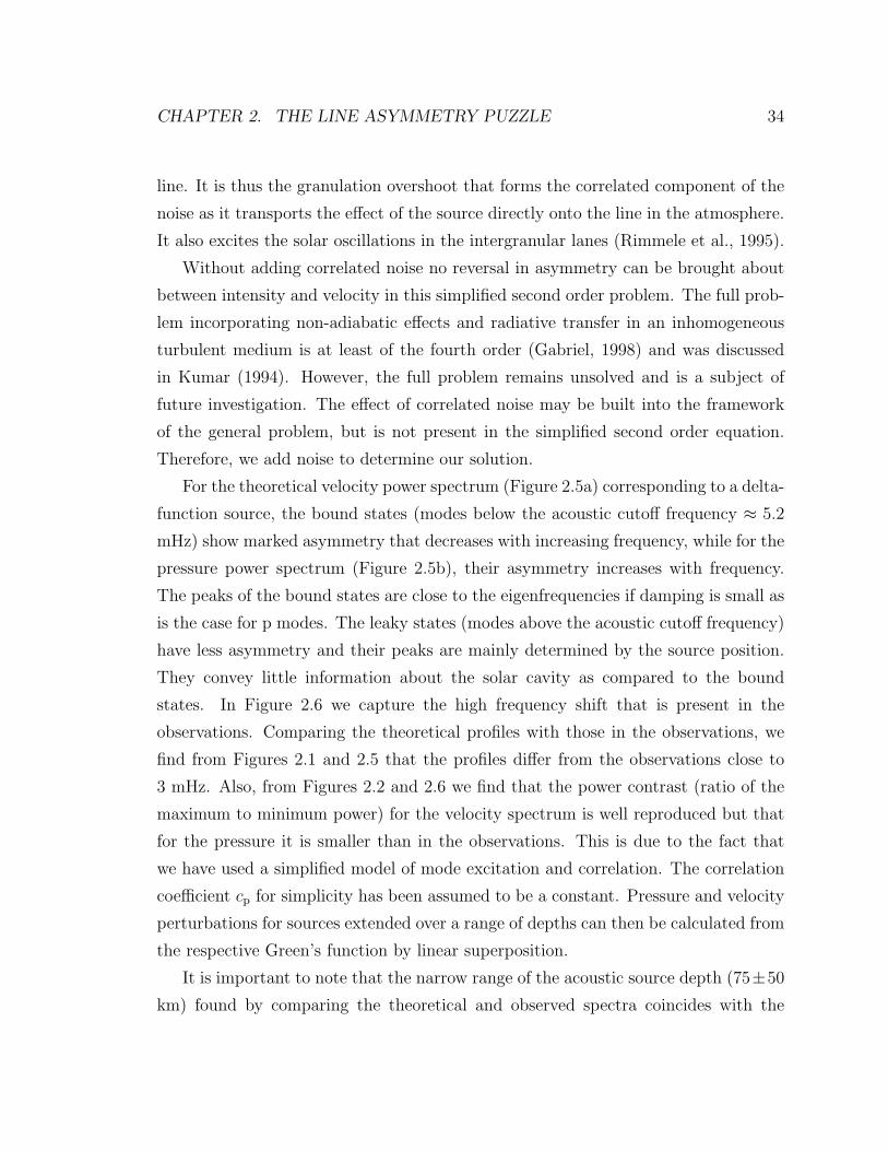
CHAPTER 2. THE LINE ASYMMETRY PUZZLE 34
line. It is thus the granulation overshoot that forms the correlated component of the
noise as it transports the effect of the source directly onto the line in the atmosphere.
It also excites the solar oscillations in the intergranular lanes (Rimmele et al., 1995).
Without adding correlated noise no reversal in asymmetry can be brought about
between intensity and velocity in this simplified second order problem. The full prob-
lem incorporating non-adiabatic effects and radiative transfer in an inhomogeneous
turbulent medium is at least of the fourth order (Gabriel, 1998) and was discussed
in Kumar (1994). However, the full problem remains unsolved and is a subject of
future investigation. The effect of correlated noise may be built into the framework
of the general problem, but is not present in the simplified second order equation.
Therefore, we add noise to determine our solution.
For the theoretical velocity power spectrum (Figure 2.5a) corresponding to a delta-
function source, the bound states (modes below the acoustic cutoff frequency ≈ 5.2
mHz) show marked asymmetry that decreases with increasing frequency, while for the
pressure power spectrum (Figure 2.5b), their asymmetry increases with frequency.
The peaks of the bound states are close to the eigenfrequencies if damping is small as
is the case for p modes. The leaky states (modes above the acoustic cutoff frequency)
have less asymmetry and their peaks are mainly determined by the source position.
They convey little information about the solar cavity as compared to the bound
states. In Figure 2.6 we capture the high frequency shift that is present in the
observations. Comparing the theoretical profiles with those in the observations, we
find from Figures 2.1 and 2.5 that the profiles differ from the observations close to
3 mHz. Also, from Figures 2.2 and 2.6 we find that the power contrast (ratio of the
maximum to minimum power) for the velocity spectrum is well reproduced but that
for the pressure it is smaller than in the observations. This is due to the fact that
we have used a simplified model of mode excitation and correlation. The correlation
coefficient cp for simplicity has been assumed to be a constant. Pressure and velocity
perturbations for sources extended over a range of depths can then be calculated from
the respective Green’s function by linear superposition.
It is important to note that the narrow range of the acoustic source depth (75±50
km) found by comparing the theoretical and observed spectra coincides with the

CHAPTER 2. THE LINE ASYMMETRY PUZZLE 35
Figure 2.6: Normalized theoretical high frequency velocity (solid curve) and pressurepower spectra (dashes) of Figure 2.4 with no additive uncorrelated noise. Correlatednoise with coefficient cp greater than a threshold value of 0.04 is responsible for therelative frequency shift that is present in the observations.
region of superadiabatic convection in the solar model (see Chapter 5). This region
represents the highly unstable upper boundary layer of the convection zone where
the convective motions are most violent. The extent of the source was determined
by comparing the high frequency peaks of the theoretical spectra with those of the
observations (Kumar and Lu, 1991), for a range of source depths.
2.2.3 Simple model of asymmetry
Solar p modes are formed by resonances of the acoustic cavity beneath the Sun’s
surface. The shape and size of the cavity depends on the stratification. However,
some basic features of line asymmetry can be explained by approximating the cavity
as a rectangular potential well V (r) of width a with an infinite potential at the lower
turning point r = 0, and a finite height at the upper turning point r = a (Stein, 1966);

CHAPTER 2. THE LINE ASYMMETRY PUZZLE 36
(Nigam and Kosovichev, 1996); (Abrams and Kumar, 1996). This height corresponds
to the square of the acoustic cutoff frequency ν2c (νc ≡ ωc/2π) while the width a relates
to the angular degree l of the mode. For simplicity the effects of stratification have
been neglected. The sound speed, c, is assumed to be constant in this problem. The
effect of damping is included in the complex frequency ω21 = (ω2 + iωΓ), the factor Γ
representing the damping coefficient and ω is the frequency. A delta-function source
is placed at r = rs inside the cavity. So, we write the reduced wave equation for the
pressure perturbation:
d2Ψ
dr2+
ω21 − V (r)
c2Ψ = δ(r − rs) (2.4)
where Ψ is proportional to the pressure perturbation.
Equation (2.4) is solved analytically (see Appendix A.3), using the boundary
condition that Ψ = 0 at r = 0 and applying the Sommerfeld radiation condition far
away from the upper turning point r = a. This gives the Green’s function GΨ for Ψ
(which is proportional to the pressure perturbation) at a particular observing point
r = robs; this can be taken to be at the upper turning point r = a without loss of
generality. If we define ω22 = (ω2
c − ω21), the Green’s function can be written as (see
Appendix A.3, equation (A.62))
GΨ(ω1) =−c sin(ω1rs/c)
ω1cos(ω1a/c) + ω2sin(ω1a/c)e−ω2(r−a)/c (2.5)
In equation (2.5) the exponential term drops out when the observing point is at r = a.
Equation (2.5) can be written as
GΨ(ω1) =Ns
Dw
(2.6)
where Ns is the numerator of the Green’s function which contains the effect of the
source and Dw is the denominator of the Green’s function which contains the effect
of the cavity.
The power spectrum can be calculated from the above equation, by taking the
absolute square of the numerator and denominator. In the numerator the maximum

CHAPTER 2. THE LINE ASYMMETRY PUZZLE 37
power occurs at the source resonance frequencies ωs, as in Figure 2.7, while in the
denominator the minimum power occurs at the well resonance frequency ωw, which
is the eigenfrequency (see Appendix A.4). The two separate resonances are due to
interference, which in the simple problem are separable. At the frequency ωw the
denominator is proportional to the damping coefficient, and this results in the peaks
seen in the power spectra. It is the mismatch between these two power spectra
from the numerator (solid curve in Figure 2.7) and the denominator (dotted curve in
Figure 2.7) that makes the overall power spectra asymmetric (solid curve in Figure
2.8). Examination of the two effects separately shows that there is no asymmetry in
either of them. A combination of the two effects leads to asymmetry. The maximum
value of the power from the Green’s function is close to the eigenfrequency. In the
neighborhood of an eigenfrequency there are three cases that can arise: (i) Source
resonance frequency ωs < ωw, this leads to negative asymmetry (ii) ωs = ωw, this leads
to zero asymmetry (symmetry) and (iii) ωs > ωw, his leads to positive asymmetry. A
physical measure of asymmetry is naturally the difference ωs−ωw. The eigenfrequency
is a characteristic of the cavity and doesn’t depend on the source position and nor on
the particular representation of the acoustic disturbance.
One can also think of the source resonance in terms of zero points, which are
the frequencies ωz for which the numerator power is zero. If we look at the Green’s
function, it is at these frequencies the function is zero (see Figures 2.7 and 2.8). At
these frequencies ωz, the overall power is zero. By adding correlated noise Ncor in
equation (2.6), we get
GΨ + Ncor =Ns + NcorDw
Dw
(2.7)
In equation (2.7) the numerator changes with respect to equation (2.6) , while
the denominator remains the same. Due to this the zero points get shifted and hence
reverse the asymmetry in the power spectrum of |GΨ + Ncor|2Reversal of asymmetry can also be brought about by changing the source location
rs or changing the source type. The asymmetry reverses whenever the source crosses a
node of the eigenfunction. Moving the source deeper and keeping everything else fixed
CHAPTER 2. THE LINE ASYMMETRY PUZZLE 38
3 4 5 6 7 8 9 10 110
0.1
0.2
0.3
0.4
0.5
0.6
0.7
0.8
0.9
1
Dimensionless Angular Frequency
Norm
alize
d po
wer
Well and Source Resonance
Figure 2.7: Normalized power (solid curve) from the numerator of the Green’s functioncontaining the effect of the source and no correlated noise. The dashes represent theeffect of the correlated noise on the numerator, while the dotted curve is due to thewell resonance, the reciprocal of the denominator of the Green’s function are plottedas a function of the dimensionless angular frequency, ωa/c. The peak is close to theeigenfrequency. The normalization is done with respect to the maximum value of thedotted curve.
reverses the asymmetry. Likewise, changing the source type (eg. monopole to dipole)
also reverses the asymmetry. However, without adding correlated noise, these effects
reverse the asymmetry in both the velocity and the pressure spectra simultaneously.
This does not explain the puzzle.
2.3 Summary
In this chapter, we have given a possible explanation for the puzzle about the opposite
sense of asymmetries between intensity and velocity power spectra. This will have
an implication on the fitting and determination of eigenfrequencies from the observed

CHAPTER 2. THE LINE ASYMMETRY PUZZLE 39
3 4 5 6 7 8 9 10 110
0.1
0.2
0.3
0.4
0.5
0.6
0.7
0.8
0.9
1
Dimensionless Angular Frequency
Norm
alize
d po
wer
Reversal of Asymmetry
Figure 2.8: Normalized power with respect to the maximum (solid curve) withoutcorrelated noise of the Green’s function, as a function of the dimensionless angularfrequency, ωa/c. Adding correlated noise shifts the zero points (the frequencies wherethe power is zero) in the power spectra and reverses the asymmetry (dashed curve).
spectra, which will in turn effect the inversions.
From our model we see that the intensity and velocity power spectra have opposite
sense of asymmetry, because the solar noise is partly correlated with the source that
is responsible for exciting the solar oscillations. The solar noise is made up of two
parts: one which is correlated to the source and the other is the additive uncorrelated
background. This also explains the appreciable frequency shift at and above the
acoustic cutoff frequency, for the high frequency pseudo-modes, which are in fact
responsible for the asymmetry of the bound states.
For a composite source the source depth is found to be in a thin layer 75 ± 50
km below the photosphere. It is remarkable that the theoretical spectra matches the
observations when the source is placed within the superadiabatic layer, thus pinning
down the location, extent and the nature of the source.

Chapter 3
Phase and Amplitude Differences(Part of this chapter is published in ApJ 1999, 510, L149)
The phase difference between velocity and intensity is also linked to the excitation
of p modes. Ground-based observations and analysis carried out by Deubner and
Fleck (1989), Deubner et al. (1992) and space-based observations from MDI that
were analyzed by Straus et al. (1998) revealed a velocity intensity a phase difference
that is below 90 degrees along modal lines of the solar p mode spectra. Above
the acoustic cutoff a non-zero phase difference is observed. But a simple adiabatic
theory of solar oscillations predicts a phase difference of 90 degrees for modes below
the acoustic cutoff frequency (bound states) and zero for modes above the acoustic
cutoff frequency (scattered states). To explain this disagreement between theory and
observations they suggested that continuous partial reflection of the waves in the solar
atmosphere was responsible for the observed phase difference. A number of authors
have studied this problem theoretically (Marmolino and Severino, 1991); (Wang et al.,
1995). However, their models could not explain the unusual phase difference between
velocity and intensity along modal lines. More recently, it was seen in the MDI data
that at low frequencies the velocity has a higher power contrast than intensity, relative
to the uncorrelated background. While at high frequencies above the acoustic cutoff,
the continuum intensity shows higher power contrast relative to the uncorrelated
background compared to the Doppler velocity, see Fig. 2.1 and Fig. 1 of Nigam et al.
(1998). In addition, a puzzling shift between the maxima in the velocity and intensity
40
CHAPTER 3. PHASE AND AMPLITUDE DIFFERENCES 41
high-frequency power spectra is observed in Fig. 2.6 (Nigam et al., 1998).
The phase difference between the intensity maximum and the radius minimum
was discovered in Cepheid pulsation many decades ago. Subsequently, this difference
(called the phase lag) has been determined for a large number of pulsating stars of
different types. In these cases the phase lag is interpreted in terms of nonadiabatic
effects and it is closely linked to the driving mechanism. Recently, Houdek et al.
(1995) presented an attempt to explain the phase lag in the solar oscillations as a
result of the nonadiabatic effects. In the solar case, this theory is far less reliable than
in the case of Cepheids.
We propose that the phase difference and variation of power in the velocity and
intensity spectra can be explained in the adiabatic approximation by the interaction
of the p modes and part of the background noise that is correlated to the source
responsible for exciting the waves. The correlated noise is also responsible for the
reversal of asymmetry between velocity and intensity (Nigam et al., 1998). This
result has been recently confirmed by Rast (1999) and Kumar and Basu (1999).
The solar intensity and velocity oscillations are usually observed from variations in
an absorption line. The intensity variations consist of two parts: solar oscillation
modes and granulation noise. Since the oscillation modes are excited by granulation,
the granulation signal (noise) is partially correlated with the oscillations. Thus, the
observed intensity and to some extent, velocity variations, have a noise component
which is caused directly by granulation and correlated to the oscillations.
3.1 Theoretical model
The Green’s function for the potential well model described in section (2.2.3) given
by equation (2.5) is (see Appendix A.3 for derivation)
GΨ(ω1) =−c sin(ω1rs/c)
ω1cos(ω1a/c) + ω2sin(ω1a/c)e−ω2(r−a)/c (3.1)
For modes below the acoustic cutoff frequency the above equation can be simpli-
fied; and, taking into account the time dependence eiωt, the pressure perturbation δp,
CHAPTER 3. PHASE AND AMPLITUDE DIFFERENCES 42
that is taken as a proxy for the intensity fluctuations in the observations which are
caused by the oscillations, is
δp ∝ −αc
ωc
eiωte−ωc(r−a)/c (3.2)
where α is a complex analytical function of ω, a, rs, c and the damping. Using the
equation of continuity, the velocity perturbation is
δv =δp ω
cρωc
eiπ/2 (3.3)
where ρ is the density which has been assumed to be constant in this simple model
(see Appendix B for details). Without loss of generality both the pressure and velocity
perturbations are evaluated at the upper turning point r = a.
The cross spectrum (see Appendix B, equation (B.13) for its definition) between
the velocity and pressure perturbations is calculated after adding correlated noise,
and is,
Svp = (δv + Nv,cor)(δp + Np,cor)∗ + Nv,uncorN
∗p,uncor (3.4)
where * refers to the complex conjugate. Np,cor and Nv,cor are the complex correlated
noise that are added to the pressure and velocity perturbations in equations (3.2) and
(3.3) respectively, and Np,uncor and Nv,uncor are the complex uncorrelated noise.
The phase of the cross spectra Svp gives the phase difference between velocity and
pressure, and is given by
θv−p = arctanNi +
ω|δp|2cρωc
Nr
(3.5)
where Nr and Ni are the real and imaginary parts of the terms in the cross spectra in
equation (3.4) that contain the correlated noise, (N∗p,corδv + Nv,corδp
∗ + Nv,corN∗p,cor +
Nv,uncorN∗p,uncor). They have dimensions of velocity times pressure.
From equation (3.5) it is evident that the phase difference θv−p is related to the
power |δp|2. Since tan is a monotonic function in (-π/2, π/2), the phase difference
rises and falls whenever the power jumps and falls, which happens whenever a mode
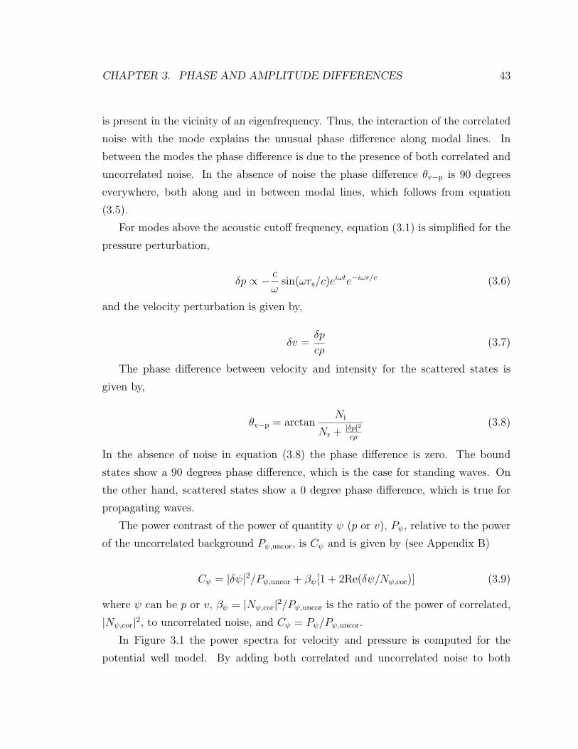
CHAPTER 3. PHASE AND AMPLITUDE DIFFERENCES 43
is present in the vicinity of an eigenfrequency. Thus, the interaction of the correlated
noise with the mode explains the unusual phase difference along modal lines. In
between the modes the phase difference is due to the presence of both correlated and
uncorrelated noise. In the absence of noise the phase difference θv−p is 90 degrees
everywhere, both along and in between modal lines, which follows from equation
(3.5).
For modes above the acoustic cutoff frequency, equation (3.1) is simplified for the
pressure perturbation,
δp ∝ − c
ωsin(ωrs/c)e
iωte−iωr/c (3.6)
and the velocity perturbation is given by,
δv =δp
cρ(3.7)
The phase difference between velocity and intensity for the scattered states is
given by,
θv−p = arctanNi
Nr + |δp|2cρ
(3.8)
In the absence of noise in equation (3.8) the phase difference is zero. The bound
states show a 90 degrees phase difference, which is the case for standing waves. On
the other hand, scattered states show a 0 degree phase difference, which is true for
propagating waves.
The power contrast of the power of quantity ψ (p or v), Pψ, relative to the power
of the uncorrelated background Pψ,uncor, is Cψ and is given by (see Appendix B)
Cψ = |δψ|2/Pψ,uncor + βψ[1 + 2Re(δψ/Nψ,cor)] (3.9)
where ψ can be p or v, βψ = |Nψ,cor|2/Pψ,uncor is the ratio of the power of correlated,
|Nψ,cor|2, to uncorrelated noise, and Cψ = Pψ/Pψ,uncor.
In Figure 3.1 the power spectra for velocity and pressure is computed for the
potential well model. By adding both correlated and uncorrelated noise to both

CHAPTER 3. PHASE AND AMPLITUDE DIFFERENCES 44
velocity and pressure, we see that the power contrast in the velocity power spectrum
is higher at low frequencies and falls off rapidly at higher frequencies in comparison
to the pressure power spectrum. To see this we assume that the correlated noise
in the velocity is negligible and set βv = 0 in equation (3.9), therefore the power
contrast for the velocity is proportional to |δv|2/Pv,uncor, which rapidly decreases at
higher frequencies, as the waves are no longer trapped. In the case of the pressure
perturbation from equation (3.9) the power contrast has additional terms involving
βp. Due to the presence of these additional terms the pressure power contrast does
not fall off rapidly as compared to the velocity power contrast. It is also seen that
the presence of correlated noise is responsible for the reversal of asymmetry and also
the high frequency shift between velocity and pressure (Nigam et al., 1998).
3.2 Comparison of the Numerical Model and Ob-
servations
Velocity and pressure perturbations are generated numerically from the Green’s func-
tion for the reduced wave equation as described in Chapter 2, (see also Appendix A.2)
using a standard solar model (Christensen-Dalsgaard et al., 1996). In order to com-
pare with the MDI observations, noise is added to the computed perturbations. We
took an example of angular degree l = 200 and angular order m = 81. Other modes
in the MDI data behave similarly. From this the cross spectrum between velocity
and pressure for the bound states is computed. The amplitude (absolute value) and
phase of the cross spectra are plotted in Figure 3.2. A similar plot is made for the
cross spectrum after smoothing the MDI data in Figure 3.3. By adjusting the noise
the observed phase jump in Figure 3.3b between velocity and intensity along modal
lines is reproduced in the theoretical plot in Figure 3.2b (black curve). The correlated
noise is close to zero in the velocity perturbation. We find that the phase difference
is below 90 degrees. While the unusual behavior of the phase along modal lines has
been explained in the discussion of equation (3.5), from which we see that in the
vicinity of an eigenfrequency the power rises and falls, and hence the phase rises and
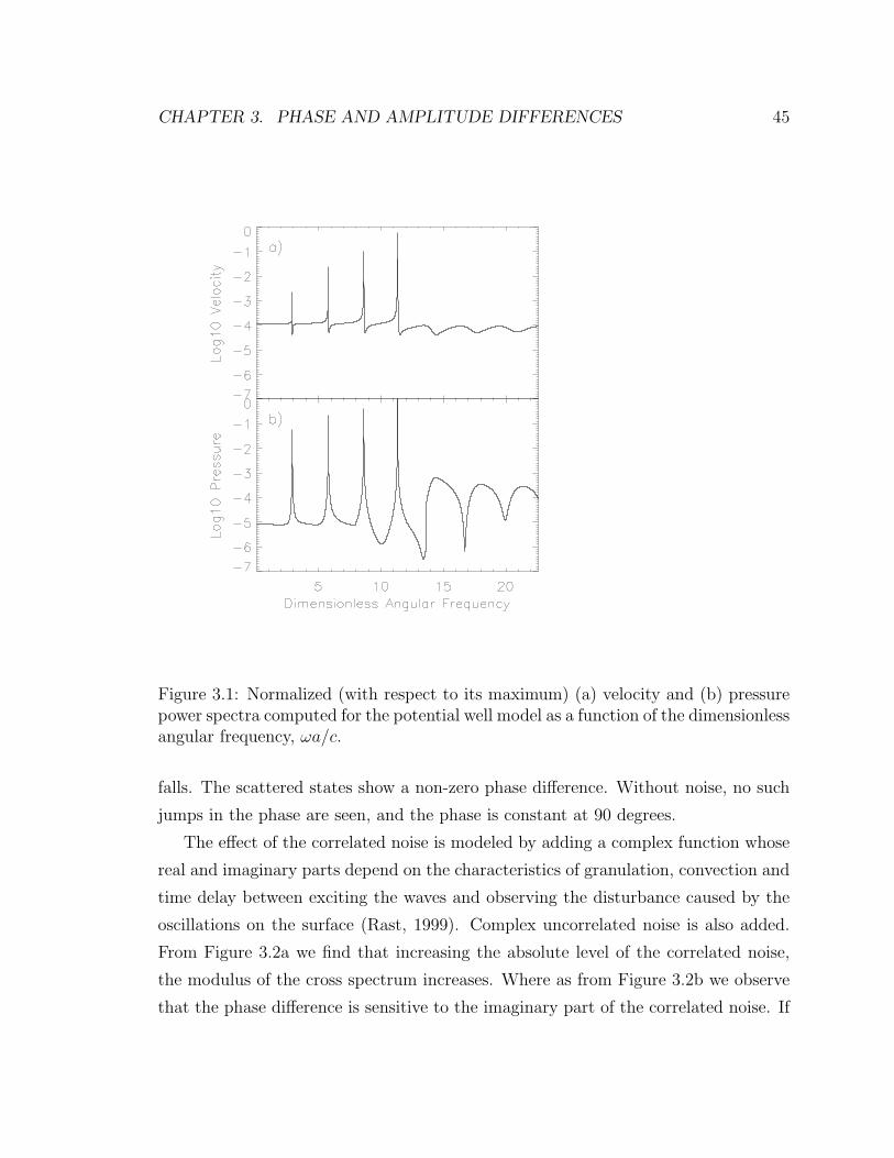
CHAPTER 3. PHASE AND AMPLITUDE DIFFERENCES 45
Figure 3.1: Normalized (with respect to its maximum) (a) velocity and (b) pressurepower spectra computed for the potential well model as a function of the dimensionlessangular frequency, ωa/c.
falls. The scattered states show a non-zero phase difference. Without noise, no such
jumps in the phase are seen, and the phase is constant at 90 degrees.
The effect of the correlated noise is modeled by adding a complex function whose
real and imaginary parts depend on the characteristics of granulation, convection and
time delay between exciting the waves and observing the disturbance caused by the
oscillations on the surface (Rast, 1999). Complex uncorrelated noise is also added.
From Figure 3.2a we find that increasing the absolute level of the correlated noise,
the modulus of the cross spectrum increases. Where as from Figure 3.2b we observe
that the phase difference is sensitive to the imaginary part of the correlated noise. If
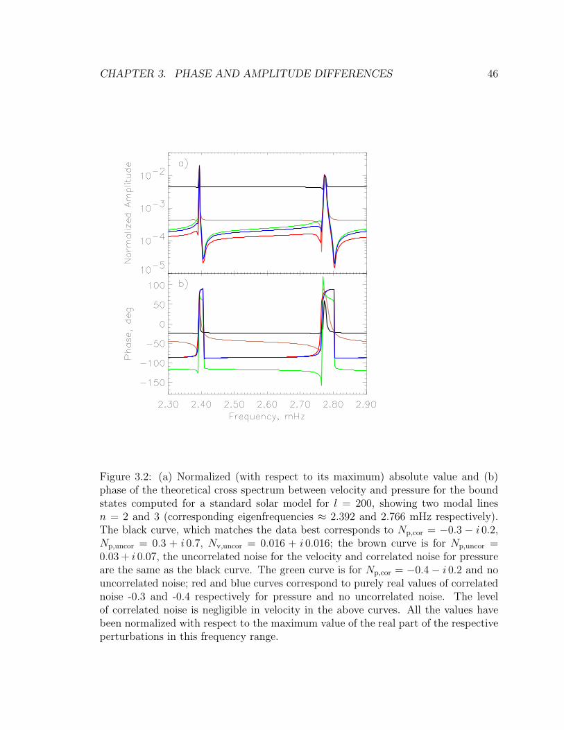
CHAPTER 3. PHASE AND AMPLITUDE DIFFERENCES 46
Figure 3.2: (a) Normalized (with respect to its maximum) absolute value and (b)phase of the theoretical cross spectrum between velocity and pressure for the boundstates computed for a standard solar model for l = 200, showing two modal linesn = 2 and 3 (corresponding eigenfrequencies ≈ 2.392 and 2.766 mHz respectively).The black curve, which matches the data best corresponds to Np,cor = −0.3 − i 0.2,Np,uncor = 0.3 + i 0.7, Nv,uncor = 0.016 + i 0.016; the brown curve is for Np,uncor =0.03 + i 0.07, the uncorrelated noise for the velocity and correlated noise for pressureare the same as the black curve. The green curve is for Np,cor = −0.4− i 0.2 and nouncorrelated noise; red and blue curves correspond to purely real values of correlatednoise -0.3 and -0.4 respectively for pressure and no uncorrelated noise. The levelof correlated noise is negligible in velocity in the above curves. All the values havebeen normalized with respect to the maximum value of the real part of the respectiveperturbations in this frequency range.
CHAPTER 3. PHASE AND AMPLITUDE DIFFERENCES 47
Figure 3.3: (a) Normalized (with respect to its maximum) absolute value and (b)phase of the cross spectrum between velocity and intensity for the smoothed SOI/MDIdata for l = 200, m = 81 showing two modal lines n = 2 and 3 as in Fig. 3.2. Thephase difference is below 90 degrees.
the imaginary part is set equal to zero, the phase difference is not sensitive to changes
in the real part, as seen by the blue and red curves, which coincide.
3.3 Summary
We have explained the unusual phase difference that is below 90 degrees between
velocity and intensity spectra. By adding correlated and uncorrelated noise we are

CHAPTER 3. PHASE AND AMPLITUDE DIFFERENCES 48
able to reproduce the phase jump along modal lines. The deviation of the phase dif-
ference from 90 degrees, that is predicted by simple adiabatic solar oscillation theory
was puzzling for many years. The phase difference depends on the power spectrum,
which jumps whenever an eigenfrequency is approached. The high frequency modes
show a non-zero phase difference which is different from the zero phase difference pre-
dicted theoretically. Taking into account the correlated noise whose level happens to
be higher in the pressure spectrum compared to the velocity, we are able to explain
the high power contrast in the velocity power spectrum at low frequencies and its
rapid drop off at frequencies above the cutoff frequency, in comparison to the inten-
sity. Studying the asymmetry, the high-frequency shift, the amplitude and the phase
difference between velocity and intensity is a useful diagnostic to measure the level
and phase of the correlated noise in the data, and also understand the mechanism of
mode excitation of solar oscillations.

Chapter 4
Asymmetric Fitting Formula(Part of this chapter is published in ApJ 1998, 505, L51 and ApJ 1998,
506, L147)
An asymmetric fitting formula is derived to measure the eigenfrequencies. The prin-
cipal goal of helioseismology is to infer the internal structure and rotation of the
Sun from the observed eigenfrequencies of the normal modes of oscillation. Solar
eigenfrequencies are generally determined by assuming that the power spectrum is
symmetric and can be fitted by a Lorentzian. This is clearly not the case. Recent
studies (Duvall et al., 1993); (Gabriel, 1993); (Abrams and Kumar, 1996); (Roxburgh
and Vorontsov, 1997); (Nigam et al., 1998); (Rosenthal, 1998) have shown that the
peaks in the power spectra are asymmetric. The asymmetry may be caused by in-
terference between an outward-directed wave from the source and a corresponding
inward-directed wave that passes through the region of wave propagation. Also im-
portant is the interaction between the wave and part of the background noise that is
correlated to the source responsible for exciting the waves. The solar intensity and
velocity oscillations are usually observed from variations in an absorption line. These
variations consist of two parts: solar oscillation modes and granulation noise. Be-
cause the oscillation modes are excited by granulation, the granulation signal (noise)
is partially correlated with the oscillations. According to Goode et al. (1998) the
solar oscillations are excited in the intergranular dark lanes. Thus, the observed in-
tensity and velocity variations have a noise component which is caused directly by
49

CHAPTER 4. ASYMMETRIC FITTING FORMULA 50
the dark lanes and correlated to the amplitude of the oscillations. The absorption
line is affected by the p mode oscillations and the solar granulation, (due to intensity
fluctuations and overshoot) which modulate and shift the line. More specifically, the
intensity fluctuations form the correlated component of the noise that is responsible
for the reversal of asymmetry in the intensity power spectrum.
Line asymmetry in the solar power spectra alters the frequencies which are ob-
tained under the assumption that the lines are symmetric. It has been observed
(Rhodes et al., 1997) that when asymmetric line profiles of the velocity data are
fitted with a symmetric formula, the resulting frequency is shifted by a significant
amount. The affect of asymmetry was first observed by Toutain (1993) and later he
observed frequency differences of the order of 0.1 µHz (Toutain et al., 1997) between
intensity and velocity, for modes of low angular degree when Lorentzian fits are per-
formed. This suggests that an asymmetric fitting formula should be used to measure
solar eigenfrequencies instead of the usual Lorentzian fits.
In §4.2 we describe an asymmetric fitting formula that was derived from a phys-
ical understanding of asymmetry. The derivation takes into account the reversal of
asymmetry between velocity and intensity when correlated noise is present in the data
(Nigam and Kosovichev, 1998). The correlated noise is above a certain threshold to
reverse the asymmetry in the intensity power spectrum but is small in the velocity
spectrum so as to preserve its asymmetry. We use a simple model to derive an an-
alytical fitting formula, as the full solar model is complicated and has to be dealt
with numerically. In §4.3 we use our formula to fit both the theoretical velocity and
pressure (intensity) spectra. This is compared with a symmetric Lorentzian fit, and
deviations from the computed theoretical eigenfrequencies are discussed. In §4.4 we
repeat the fits for the medium l MDI data and in §4.5 they are applied to the low l
data from MDI and VIRGO instruments.
4.1 Derivation of the Formula
The Green’s function for the potential well model from equation (2.5) in chapter 2 is

CHAPTER 4. ASYMMETRIC FITTING FORMULA 51
GΨ(ω1) =−c sin(ω1rs/c)
ω1cos(ω1a/c) + ω2sin(ω1a/c)e−ω2(r−a)/c (4.1)
A new formula to fit the bound states (modes with frequencies less than the
acoustic cutoff frequency) is derived from equation (4.1). In the derivation it is
assumed that the damping is much smaller than the frequency, which is true of
the solar p modes. We next substitute the expressions for ω1 and ω2 into equation
(4.1), and expand for small Γ. Making use of the eigenvalue condition at ω = ω0:
ω cos(ωa/c) + w sin(ωa/c) = 0, (where w2 = ω2c − ω2) (see Appendix A.4) we get
the complex amplitude of the pressure perturbation AΨ (see Appendix C.1, equation
(C.25))
AΨ(X) = −Aw
sin(βX − pw) + i2β cos(βX − pw)
sin(βX) + i2β cos(βX)
(4.2)
Here X = (ω − ω0)/Γ, β = aΓ/c, Aw = A0c/ωc, A0 is the mode amplitude that
has been multiplied by the Green’s function, pw = p0 +φc, p0 = ω0ds/c, sin φc ≈ ω/ωc
and ds = a− rs is the depth of the source below the upper turning point. To explain
the reversal of asymmetry between velocity and intensity (equivalent to the pressure
perturbation), correlated noise Ncor which is due to the granulation is added to the
amplitude signal AΨ (Nigam and Kosovichev, 1998). The power is then given by
P = |Ncor + AΨ|2. This gives a trigonometric expression for the power, that can be
used to fit the peaks and troughs (minimum points in the power spectra) in the power
spectra (see Appendix C.1, equation (C.28)) and is
P (x) ≈ A[U cos(Ux) + B sin(Ux)]2 + B2U2 cos2(Ux)
U2 cos2(Ux) + sin2(Ux)(4.3)
Where x = 2(ν − ν0)/γ, cyclic frequency ν = ω/2π, γ = Γ/2π,A = 4A2w(1− q2
w)β−2,
B = 0.5β(Ncor − Awqw)A−1w (1− q2
w)−1/2, qw = cos pw and U = β/2 is a dimensionless
quantity. Here β is the product of the damping Γ (mode line width) and the travel
time a/c of the p modes between the upper and lower turning points. U is generally
small for the solar case. The trigonometric formula in equation (4.3) can be used to
fit multiple peaks, in this case the travel time can be written in terms of the mode

CHAPTER 4. ASYMMETRIC FITTING FORMULA 52
spacing ∆ν between radial orders of constant angular degree l. The expression for U
is πγ/2∆ν.
This expression for the power can be expanded for small Ux to give a more prac-
tical polynomial formula,
P (x) ≈ A(1 + Bx)2 + B2
1 + x2+ Bl (4.4)
Here Bl is the uncorrelated linear background and Ncor is the correlated noise. In
using equation (4.4) as a fitting formula for the line profile the fit parameters are A,B,
the damping γ (which is related to the mode linewidth), and the eigenfrequency ν0.
The parameter B controls the asymmetry. It is positive for positive asymmetry (more
power on the higher frequency end of the peak) and negative for negative asymmetry
(more power on the lower frequency end of the peak). It contains the effects of
correlated noise and the source, the two factors that are responsible for asymmetry.
The sign of B changes when Ncor changes sign. When B = 0 (absence of asymmetry)
the first term in equation (4.4) reduces to the usual Lorentzian profile. Without
correlated noise the frequencies of the troughs in the power spectra are determined
by the source characteristics and the solar structure. Adding correlated noise shifts
these frequencies.
Other workers have derived fitting formulae (Duvall et al., 1993); (Gabriel, 1995);
(Appourchaux et al., 1995b); (Abrams and Kumar, 1996); (Rhodes et al., 1997);
(Rosenthal, 1998), but their models do not explain the reversal of asymmetry between
velocity and intensity. For instance, the polynomial line fitting formula derived by
Rosenthal (1998), equation (45), is different from our formula in equation (4.4), as
his formula does not contain correlated noise, which is responsible for the reversal of
asymmetry between intensity and velocity. Other important features of our profile,
equation (4.4) are that it is always positive and as shown below matches the theoretical
power spectra from a standard solar model and the MDI observations quite well.

CHAPTER 4. ASYMMETRIC FITTING FORMULA 53
4.2 Fitting of Velocity and Pressure Theoretical
Power Spectra
A simultaneous fit of the velocity and pressure spectra of angular degree l = 200
is performed using the above formula. The fitting is carried out using a standard
nonlinear minimization algorithm. We minimize the chi-square error, defined as the
square of the difference between the power estimated by the above formula and that
from the theoretical power spectra, summed over a suitable frequency range so as to
isolate the mode (see Appendix C.2). The theoretical power spectra are generated
from the Green’s function for the reduced wave equation as described in Nigam et al.
(1998). For modes of medium angular degree l, the effects of spherical geometry can
be neglected. In the plane parallel approximation, the reduced wave equation can be
written using equations (1.30) and (1.43)
d2Ψ
dr2+
ω21 − ω2
+
c2Ψ = S[f , q], (4.5)
where Ψ is proportional to the Lagrangian pressure perturbation δp, r is the radius, ω
is the frequency and c is the equilibrium sound speed. In equation (4.5) ω2+ plays the
role of the acoustic potential (Gough, 1993) and is calculated from a solar model using
equation (1.38). For the acoustic modes we neglect ω2− in equation (1.37), as it is very
small compared to ω2+. Both ω+ and c are functions of radius. S is a combination
of source terms that include the fluctuating Reynolds stress force, f , and the mass
source, q. The Green’s function GΨ(r, rs) of equation (4.5), for a delta-function source
at r = rs is found numerically using a standard solar model (Christensen-Dalsgaard
et al., 1996). We use reflecting boundary conditions at the lower and upper turning
points. To the Green’s function we add the noise Ncor(ν), which is correlated with the
source function s(ν), and uncorrelated noise Bl(ν). One then obtains for the pressure
perturbation, which serves as a proxy for the intensity observations.
p(ν) = s(ν)[Ncor(ν) + Gp(ν)] + Bl(ν) (4.6)

CHAPTER 4. ASYMMETRIC FITTING FORMULA 54
Figure 4.1: Asymmetrical fit for the l = 200, n = 5 theoretical power spectra (logscale) that has been normalized with respect to its maximum value: (a) Velocityspectrum and (b) Pressure spectrum. The dashed lines show the computed eigen-frequency. The fitted profile is indistinguishable from the theoretical profile, with amaximum deviation of 0.003%.

CHAPTER 4. ASYMMETRIC FITTING FORMULA 55
Figure 4.2: (a) Squares denote the deviation (in nHz) of the asymmetrical fittedfrequencies from the computed eigenfrequencies, triangles are the deviation of theLorentzian fitted frequencies of the theoretical pressure power spectrum for l = 200and the diamonds are the deviation of the Lorentzian fitted frequencies of the ve-locity power spectrum from the computed eigenfrequencies. (b) Triangles representthe dimensionless asymmetry parameter B for the pressure power spectrum and thediamonds for the velocity power spectrum.

CHAPTER 4. ASYMMETRIC FITTING FORMULA 56
where Gp is proportional to GΨ. The power spectrum for the pressure perturbation
is calculated from the function p(ν), see Fig. 2.5b. This equation is same as equation
(2.3) in chapter 2 with Bl(ν) = np(ν). The velocity power spectrum is found in a
similar manner, from the complex velocity amplitude (Appendix D, equation (D.25)).
The eigenfrequencies ω0 of the solar model are determined numerically from equa-
tion (4.5) with no source term (see Appendix C.3).
The first five modes (bound states with frequencies less than the acoustic cutoff
frequency) of the two spectra are fitted using both the asymmetrical formula and
the Lorentzian profile. The fitting algorithm converges rapidly to the same fitted fre-
quency for both the velocity and pressure power spectra when the asymmetric formula
is used. This is not the case for the Lorentzian fits, where the convergence is slow.
The asymmetrical fit for n = 5 is shown, along with the computed eigenfrequency, in
Figure 4.1. The fits are indistinguishable from the theoretical spectra, with a max-
imum deviation of 0.003%. The resulting fitted frequencies are then compared with
the computed eigenfrequencies in Figure 4.2a. We see the deviation from the true
eigenfrequencies is more pronounced for the Lorentzian fit than for the asymmetrical
formula, which yields values very close to the eigenfrequencies.
In Figure 4.2b we show the asymmetry parameter B for the five modes. The
asymmetry parameter is negative for the velocity and positive for the pressure power
spectra. This difference in asymmetry is also observed in real solar power spectra.
The good agreement obtained using equation (4.4) as a fitting formula means
that the formula although derived for a simple potential, is sufficiently accurate for a
realistic solar model.
4.3 Fitting of Velocity and Intensity MDI Power
Spectra
To carry out a simultaneous fit of the m-averaged velocity and intensity spectra we
compute spherical harmonic transforms (SHTs) of full disk velocity and intensity
images from the MDI instrument (Scherrer et al., 1995). After filling gaps in the
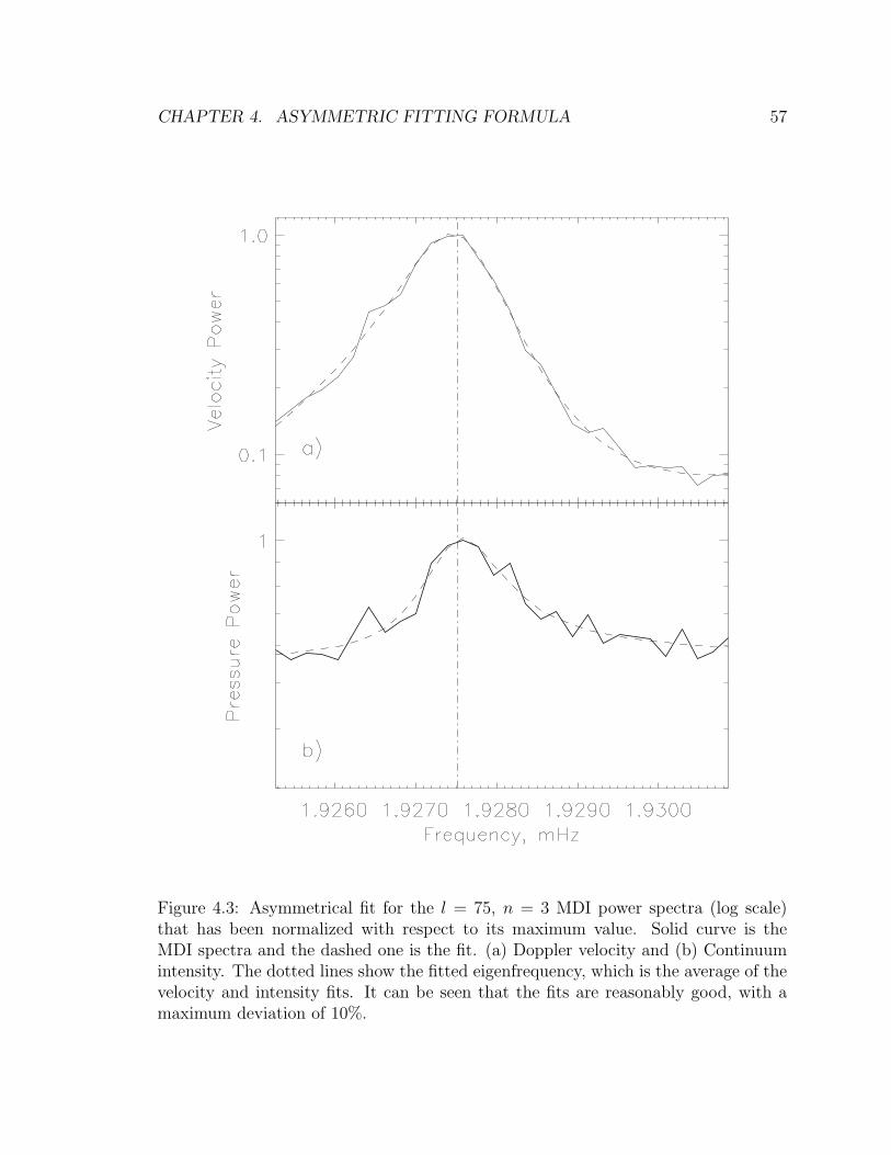
CHAPTER 4. ASYMMETRIC FITTING FORMULA 57
Figure 4.3: Asymmetrical fit for the l = 75, n = 3 MDI power spectra (log scale)that has been normalized with respect to its maximum value. Solid curve is theMDI spectra and the dashed one is the fit. (a) Doppler velocity and (b) Continuumintensity. The dotted lines show the fitted eigenfrequency, which is the average of thevelocity and intensity fits. It can be seen that the fits are reasonably good, with amaximum deviation of 10%.

CHAPTER 4. ASYMMETRIC FITTING FORMULA 58
Figure 4.4: (a) Squares denote the difference (in nHz) between the asymmetricalfitted frequencies of intensity with velocity, while the diamonds are the deviation ofthe corresponding Lorentzian fitted frequencies of the MDI power spectra for l = 75.(b) Triangles represent the dimensionless asymmetry parameter B for the intensitypower spectrum and the diamonds for the velocity power spectrum.
CHAPTER 4. ASYMMETRIC FITTING FORMULA 59
SHTs, they are Fourier transformed to make power spectra, shifted in frequency
according to a solar rotation law, and averaged over the angular order m. To simplify
the comparison we choose the 60 days from April 14 to June 12, 1997 for which
simultaneous velocity and intensity images were available.
A fit of these power spectra for angular degree l = 75 and order n from 3 to 8 is
done using the asymmetrical formula. The technique is similar to that described in
the previous section. Here we do not present the fits for l = 200 because the peaks are
not properly resolved and the fits get corrupted by the l-leakage. In Figure 4.3 we see
that the asymmetric formula fits the data reasonably well with a maximum deviation
of 10%. From the fits we get a small difference in the frequency between velocity
and intensity, which is much smaller than that obtained by fitting a Lorentzian as
seen in Figure 4.4a. In Figure 4.4b the asymmetry parameter B for both velocity
and intensity is shown. This parameter, which controls the asymmetry, is found to
decrease with frequency and reaches a minimum around 3 mHz. This is consistent
with the low l fits of Toutain et al. (1998) using the same asymmetrical formula.
4.4 Application of the formula to low degree modes
An accurate determination of frequencies of solar acoustic (p) modes of low angular
degree l is necessary to infer the structure and rotation of the solar core. Since the
work of Duvall et al. (1993) based on oscillation spectra averaged over the azimuthal
order, m, the line shape of medium-l p modes have been considered to be possibly
asymmetric. Moreover, this asymmetry showed up with opposite sign for modes
observed in intensity and in velocity. In standard techniques of measuring solar
frequencies (Anderson et al., 1990) the asymmetry is not taken into account, and the
line shape is assumed to be a Lorentzian. This leads to systematic errors in frequency
measurements, and thus to errors in helioseismic inferences of the structure of the
Sun. Recently, Toutain et al. (1997) have observed frequency differences of the order
of 0.1 µHz between intensity and velocity low-degree p mode lines when a Lorentzian
fit was done. In this chapter we show that these frequency differences can significantly
be reduced using our model of an asymmetrical line profile.
CHAPTER 4. ASYMMETRIC FITTING FORMULA 60
The first successful attempt to detect the asymmetry of low-l modes was made by
Toutain (1993) using the intensity data from the IPHIR space experiment (Frohlich
et al., 1990). However, the IPHIR data being the longest intensity time series avail-
able at that time, had a poor resolution and signal-to-noise ratio to make reliable
conclusions about the asymmetry and corresponding frequency corrections.
The oscillations of the Sun have been observed continuously for about 2 years with
three experiments on board SOHO. Two of these experiments are VIRGO (Frohlich
et al., 1995) which is measuring oscillations of the solar irradiance with a triple Sun-
photometer (SPM) and a 16-pixel imager LOI, (Appourchaux et al., 1995a) and the
MDI which is measuring with a CCD detector velocity oscillations in the Ni 6768
line (Scherrer et al., 1995). We have used the longest available time series from both
experiments consisting of 610 days of integrated velocity and spectral irradiance (at
400, 500 and 862 nm) to accurately measure the parameters of the p modes for degrees
l=0,1 and 2 in a frequency domain ranging from 2000 to 4000 µHz.
We discuss the fact that the shape of low-degree p mode lines significantly depart
from a Lorentzian profile. We use a theoretical model by Nigam and Kosovichev
(1998) to fit the asymmetrical shape found in the data. We fit both intensity and
velocity lines to determine the frequency dependence of the asymmetry and present
new estimates of eigenfrequencies of low-degree modes (Toutain et al., 1998) which are
particularly important for determining the structure of the Sun’s energy-generating
core.
4.4.1 Integrated velocity and intensity power spectra
The power spectra of the 610-day time series are plotted in Figure 4.5 in a frequency
range spanning from 1000 to 5000 µHz. Below 2000 µHz we hardly see p mode
lines in the intensity data because of granulation noise which steeply increases, and
above 4000 µHz, mode linewidths are such that modes of degrees 0 and 2 overlap. We
therefore restrict ourselves to work in this frequency range to compare the results from
the velocity and intensity data. Because of the stochastic nature of solar oscillations,
the power in each frequency bin of a line is distributed with a large variance around its
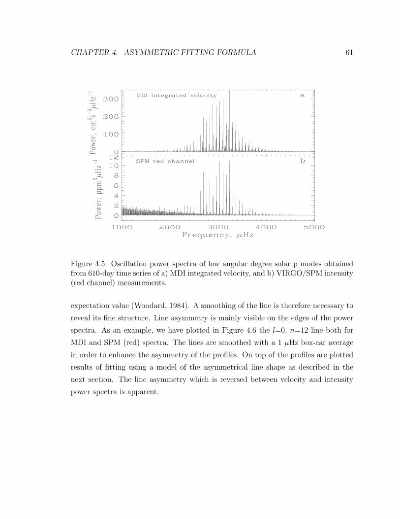
CHAPTER 4. ASYMMETRIC FITTING FORMULA 61
Figure 4.5: Oscillation power spectra of low angular degree solar p modes obtainedfrom 610-day time series of a) MDI integrated velocity, and b) VIRGO/SPM intensity(red channel) measurements.
expectation value (Woodard, 1984). A smoothing of the line is therefore necessary to
reveal its fine structure. Line asymmetry is mainly visible on the edges of the power
spectra. As an example, we have plotted in Figure 4.6 the l=0, n=12 line both for
MDI and SPM (red) spectra. The lines are smoothed with a 1 µHz box-car average
in order to enhance the asymmetry of the profiles. On top of the profiles are plotted
results of fitting using a model of the asymmetrical line shape as described in the
next section. The line asymmetry which is reversed between velocity and intensity
power spectra is apparent.
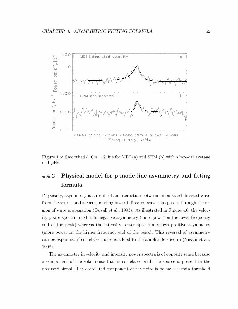
CHAPTER 4. ASYMMETRIC FITTING FORMULA 62
Figure 4.6: Smoothed l=0 n=12 line for MDI (a) and SPM (b) with a box-car averageof 1 µHz.
4.4.2 Physical model for p mode line asymmetry and fitting
formula
Physically, asymmetry is a result of an interaction between an outward-directed wave
from the source and a corresponding inward-directed wave that passes through the re-
gion of wave propagation (Duvall et al., 1993). As illustrated in Figure 4.6, the veloc-
ity power spectrum exhibits negative asymmetry (more power on the lower frequency
end of the peak) whereas the intensity power spectrum shows positive asymmetry
(more power on the higher frequency end of the peak). This reversal of asymmetry
can be explained if correlated noise is added to the amplitude spectra (Nigam et al.,
1998).
The asymmetry in velocity and intensity power spectra is of opposite sense because
a component of the solar noise that is correlated with the source is present in the
observed signal. The correlated component of the noise is below a certain threshold

CHAPTER 4. ASYMMETRIC FITTING FORMULA 63
to preserve the asymmetry obtained by the model (Nigam et al., 1998) in the velocity
power spectrum but that it is large enough (the correlated component is above a
certain threshold) to reverse the asymmetry in the intensity spectrum. This is due
to the fact that the correlated noise shifts the zero points in the amplitude spectra
of the pressure perturbation. The uncorrelated noise plays no role in the reversal of
asymmetry because it adds to the power not to the amplitude spectrum.
The solar intensity and velocity oscillations are observed from variations in an
absorption (Fraunhofer) line or, as in the case of the SPM, from intensity variations
in relatively broad bands of the solar spectrum. These variations consist of two
parts: solar oscillation modes and granulation noise. Because the oscillation modes
are excited by granulation the granulation signal (noise) is partially correlated with
the oscillations. According to Goode et al. (1998) the solar oscillations are excited
in the intergranular dark lanes. Thus, the observed intensity variations have a noise
component which is caused directly by the dark lanes and correlated to the amplitude
of the oscillations. It has been suggested by Roxburgh and Vorontsov (1997) that the
granulation overshoot forms the correlated component of the noise to the velocity
signal. However, the observations show higher level of noise in the intensity data,
and support the idea by Nigam et al. (1998) that the line asymmetry in the intensity
power spectra is reversed due to the correlated noise in the intensity observations.
To measure the properties of solar oscillations we employed an asymmetric fitting
formula of Nigam and Kosovichev (1998) for the power, P from equation (4.4):
4.4.3 Line asymmetry
According to the line shape model described in the previous section we have fitted
l=0-2 doublets and the l=1 lines between 2000 and 4000 µHz. The technique of fitting
is a standard maximum likelihood technique. Usually for a disk-averaged spectrum
we fit simultaneously the line for l=0 and 2 because they overlap. We therefore
give a mean asymmetry for these degrees. The modes of l=1 are fitted assuming
2-component rotationally split multiplets of m=1 and -1, both components having
the same asymmetry coefficient. The asymmetry coefficient is plotted in Figure 4.7

CHAPTER 4. ASYMMETRIC FITTING FORMULA 64
Figure 4.7: Asymmetry coefficient B for l = 0 (squares), l = 1 (crosses) and l = 2(diamonds) modes as a function of mode frequency for a) MDI, b) SPM data, and c)IPHIR data.

CHAPTER 4. ASYMMETRIC FITTING FORMULA 65
as a function of frequency for the MDI (a) and SPM (b) data. It is clear from these
results that, according to the definition of asymmetry we have, velocity lines exhibit
negative asymmetry whereas intensity lines exhibit positive asymmetry. Moreover the
frequency dependence of the asymmetry is similar in both cases. Asymmetry seems
to have a minimum around 3000 µHz and appears to be smaller for the velocity than
for the intensity at least for low and high frequencies. Both effects can easily be
explained if correlation with noise along with the source exciting the modes is the
factor of asymmetry (Nigam et al., 1998). In this case for a given correlation the
asymmetry is a function of the square root of the inverse of the signal-to-noise ratio,
which is largest around 3000 µHz and is bigger in general for the velocity spectra
compared to the intensity spectra, we expect the above behavior of the asymmetry
with frequency and data type. These arguments also explain why lines in the red
spectrum have slightly larger asymmetries compared to those from the SPM green
channel spectrum. This is because the signal-to-noise ratio in the red is about 10%
lower than in the green. On the other hand, blue and green signals are very well
correlated and have the same signal-to-noise ratios leading to the same asymmetry.
It is interesting to compare these asymmetries with those obtained with IPHIR
(Frohlich et al., 1990), which is an instrument similar to the SPM/VIRGO instrument.
IPHIR lines were fitted with an empirical line shape formula (Toutain, 1993) which
has the property to describe well the asymmetrical profile shown by Duvall et al.
(1993). Compared to SPM, IPHIR data have a signal-to-noise ratio in power which
is 3 times smaller. If the noise were to be solar noise and according to our model of
noise-source correlation we would expect the asymmetries with IPHIR to be 2 times
larger than with SPM, and that is what they are. It is interesting to note that an
increase in solar noise for a fixed line amplitude should mask the line asymmetry, but
it turns out to be opposite with IPHIR. The asymmetries from the IPHIR data are
generally larger than the SPM asymmetries. It is therefore consistent to think that
IPHIR noise in the 5-minute range is solar noise and that the p mode amplitudes are
correlated with the noise.
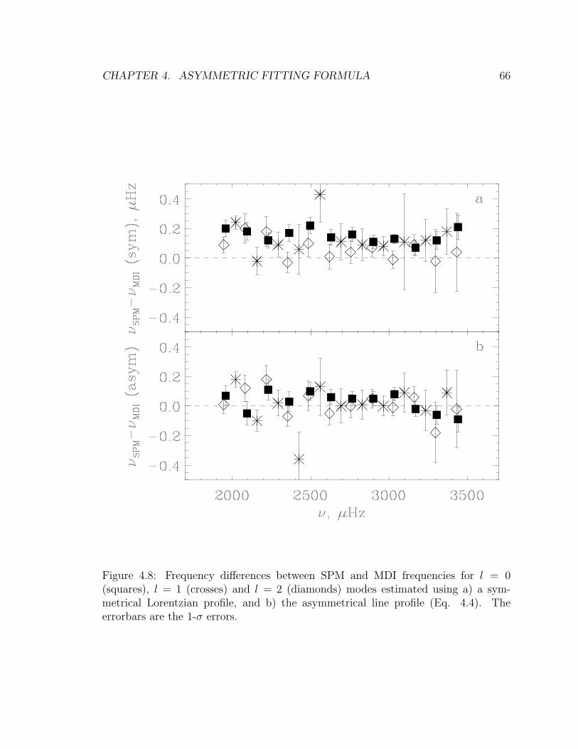
CHAPTER 4. ASYMMETRIC FITTING FORMULA 66
Figure 4.8: Frequency differences between SPM and MDI frequencies for l = 0(squares), l = 1 (crosses) and l = 2 (diamonds) modes estimated using a) a sym-metrical Lorentzian profile, and b) the asymmetrical line profile (Eq. 4.4). Theerrorbars are the 1-σ errors.
CHAPTER 4. ASYMMETRIC FITTING FORMULA 67
4.4.4 Frequency differences
The frequency differences from our symmetrical (Lorentzian) fits to the MDI and
SPM red channel data are plotted in Figure 4.8a. There is a systematic shift both for
l=0-2 and l=1 frequencies. The frequencies inferred from the SPM intensity spectrum
are systematically higher than the frequencies from the MDI velocity spectrum, as
one would expect due to the reversal of line asymmetry. These differences are of the
order of 0.1 µHz.
Using the asymmetrical formula given in equation (4.4) we have recomputed the
mode frequencies. The results are plotted in Figure 4.8b. Obviously, the differences
are significantly reduced when an asymmetrical profile is used. We have tested the
statistical significance of the asymmetry using the likelihood ratio-test (Appourchaux
et al., 1995a) and find that it is highly significant in most cases. Table 1 in Toutain
et al. (1998) shows mean frequency differences between intensity and velocity data
obtained with both symmetrical and asymmetrical fits. The close agreement between
frequencies from the asymmetrical fits means that these frequencies provide more
accurate approximation to the solar mode eigenfrequencies than the frequencies pre-
viously measured with a symmetrical Lorentzian profile. In Table 2 of Toutain et
al. (1998), a list of the frequencies obtained from the asymmetrical fits to the MDI
velocity spectra in the range from 1000 to 4000 µHz are provided.
4.4.5 Implications for solar core structure
To determine the hydrostatic structure of the Sun we combined the frequencies of
the low-degree modes with the frequencies of l = 3 − 300 obtained by Rhodes et al.
(1997) from the MDI medium-l data. The medium-l frequencies which constrain the
structure outside the solar core have not been corrected for the asymmetry effect.
The spherically symmetric structure of the Sun was determined by using a version of
the optimally localized averaging inversion method of Gough and Kosovichev (1988).
Figure 4.9 shows the relative difference between the square of the sound speed in the
Sun and the standard solar model (Christensen-Dalsgaard et al., 1996) In the central
core, the sound speed determined using the frequencies from the asymmetrical fits
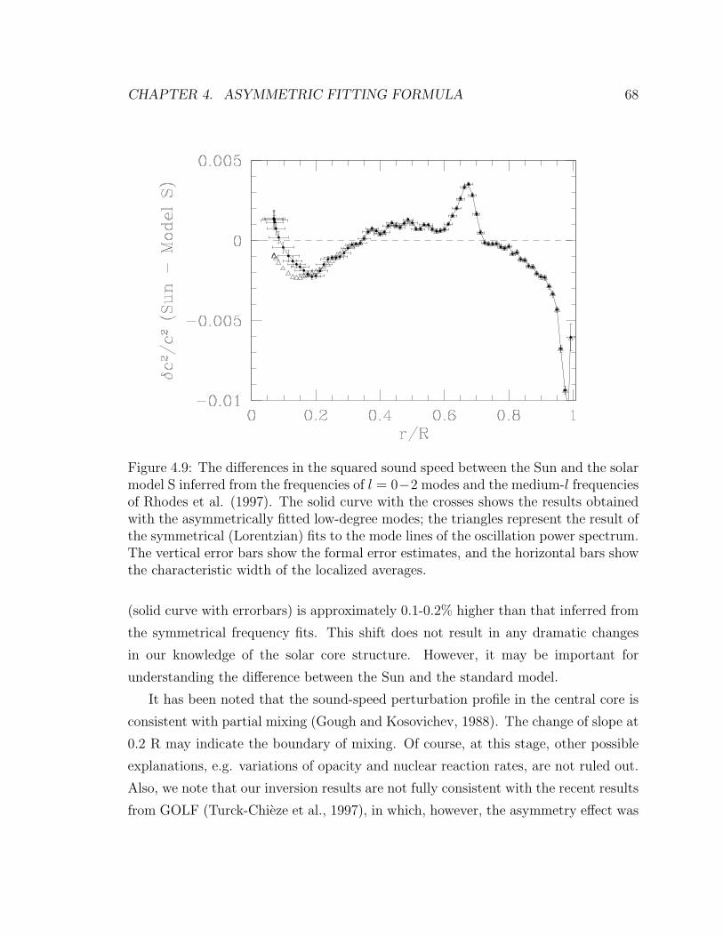
CHAPTER 4. ASYMMETRIC FITTING FORMULA 68
Figure 4.9: The differences in the squared sound speed between the Sun and the solarmodel S inferred from the frequencies of l = 0−2 modes and the medium-l frequenciesof Rhodes et al. (1997). The solid curve with the crosses shows the results obtainedwith the asymmetrically fitted low-degree modes; the triangles represent the result ofthe symmetrical (Lorentzian) fits to the mode lines of the oscillation power spectrum.The vertical error bars show the formal error estimates, and the horizontal bars showthe characteristic width of the localized averages.
(solid curve with errorbars) is approximately 0.1-0.2% higher than that inferred from
the symmetrical frequency fits. This shift does not result in any dramatic changes
in our knowledge of the solar core structure. However, it may be important for
understanding the difference between the Sun and the standard model.
It has been noted that the sound-speed perturbation profile in the central core is
consistent with partial mixing (Gough and Kosovichev, 1988). The change of slope at
0.2 R may indicate the boundary of mixing. Of course, at this stage, other possible
explanations, e.g. variations of opacity and nuclear reaction rates, are not ruled out.
Also, we note that our inversion results are not fully consistent with the recent results
from GOLF (Turck-Chieze et al., 1997), in which, however, the asymmetry effect was
CHAPTER 4. ASYMMETRIC FITTING FORMULA 69
not taken into account.
4.5 Summary
We have investigated the shape of spectral lines of solar oscillation modes using both
theoretical models and observational data from SOHO/MDI. A new fitting formula
for the power spectra of solar velocity and intensity oscillations has been derived. It
has been shown that the formula provides an accurate estimate of the eigenfrequencies
when applied to simulated and MDI velocity and intensity power spectra.
We have studied p mode frequency differences between velocity and intensity data
using 610 days of MDI integrated velocity and VIRGO/SPM intensity. Fitting l=0-2
p mode lines with commonly used Lorentzian profiles leads to systematic frequency
differences of the order of 0.1 µHz between intensity and velocity and also to a smaller
extent between different wavelengths in intensity. Using instead a model of an asym-
metrical line profile based on excitation of solar oscillations by a localized source
and its correlation with the solar noise in the observed velocity and intensity sig-
nals gives frequency differences which are significantly smaller than the differences
resulting from Lorentzian fits. The asymmetrical line profile provides more accurate
estimates of the eigenfrequencies of solar oscillations. The asymmetry effect results
in small (0.1-0.2%) but significant changes in the inferred sound-speed inversion in
the energy-generating core, which may be important for understanding the physical
processes in the core.

Chapter 5
Source of Solar Acoustic Modes(Part of this chapter is published in ApJ 1999, 514, L53)
Solar oscillations are thought to be excited stochastically by turbulent convection.
It was Lighthill (1952) who for the first time laid down a mathematical theory of
excitation of sound waves by sources of different multipoles. Since then, several
authors (Goldreich and Kumar, 1990); (Balmforth, 1992) have applied his theory to
the excitation of solar p modes. Recently, Goldreich et al. (1994) and Stein and
Nordlund (1998) argue that entropy fluctuations, which correspond to a monopole
source, drive the solar p modes.
Only recently has it been realized that the observed difference in asymmetry be-
tween velocity and intensity power spectra of the solar acoustic modes is a consequence
of the excitation mechanism of the solar oscillations. The relation of the observed
asymmetry and the excitation mechanism (Roxburgh and Vorontsov, 1997); (Nigam
et al., 1998); (Nigam and Kosovichev, 1999b); (Rast, 1999) and (Kumar and Basu,
1999) throws light on the nature of the correlated noise that is responsible for the op-
posite asymmetry between velocity and intensity. The correlation is expected because
the main source of noise is the turbulent convection which also drives the oscillations.
The same correlated noise also explains the unusual phase difference between veloc-
ity and intensity oscillations (Nigam and Kosovichev, 1999a) and the high-frequency
shift above the acoustic cutoff frequency between velocity and intensity (Nigam et al.,
1998).
70
CHAPTER 5. SOURCE OF SOLAR ACOUSTIC MODES 71
In this chapter we investigate the power spectra of velocity and pressure perturba-
tions obtained for different source depths and types. In order to explain the reversal
of asymmetry between velocity and intensity, correlated noise is added to the ampli-
tude spectrum of the pressure perturbation following Nigam et al. (1998). Previously
Kumar and Lu (1991) proposed that the source depth can be determined solely by
matching the high frequency spectra (above the acoustic cutoff frequency) with the
observed spectra. Clearly this is not the case and has been pointed out in Abrams and
Kumar (1996), Nigam et al. (1998) and Kumar and Basu (1999). In this paper the
source depth and type are determined by studying both the low and high frequency
part of the spectra. The interaction of the correlated noise and the p modes support
the observations of Goode et al. (1998), that the solar oscillations are excited in the
intergranular dark lanes.
In §2 we compute the power spectra for different source depths and for different
multipoles using a standard solar model (Christensen-Dalsgaard et al., 1996). In §3we discuss the origin and role of the correlated noise and propose a mechanism for
the excitation of solar oscillations that is consistent with the MDI observations.
5.1 Theoretical Model
We assume that solar acoustic waves are generated by turbulence in the convection
zone, and apply Lighthill’s (1952) method to calculate the velocity and pressure
perturbations. We also assume that the intensity variations recorded by the MDI
instrument correspond to the pressure perturbations together with the correlated
noise.
From equation (2.1)
d2Ψ
dr2+
[ω2 − ω2
c
c2− L2
r2
(1− N2
ω2
)]Ψ = S[f , q], (5.1)
where Ψ is proportional to the Lagrangian pressure perturbation δp, r is radius, ω is
frequency, ωc is the acoustic cutoff frequency, c is the equilibrium sound speed, N is
the buoyancy frequency, L =√
l(l + 1), S is a combination of the source terms given
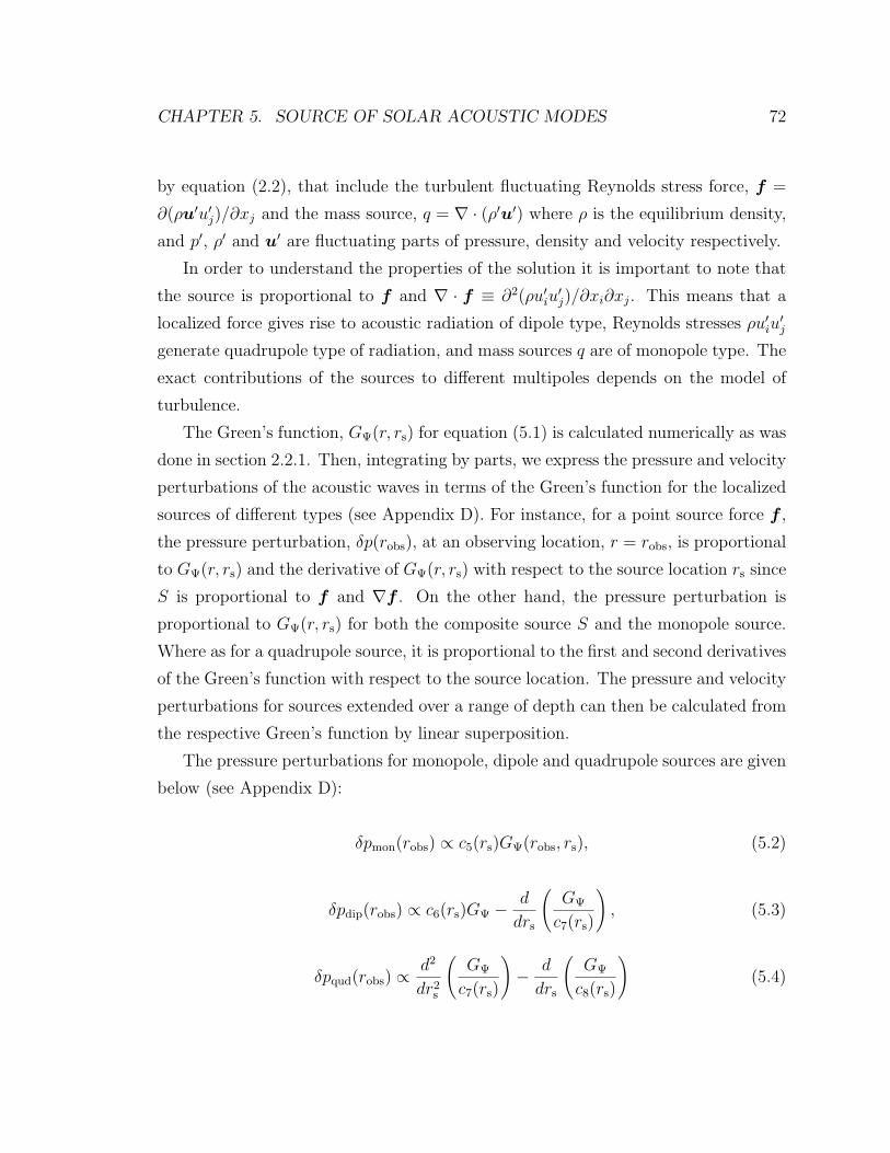
CHAPTER 5. SOURCE OF SOLAR ACOUSTIC MODES 72
by equation (2.2), that include the turbulent fluctuating Reynolds stress force, f =
∂(ρu′u′j)/∂xj and the mass source, q = ∇ · (ρ′u′) where ρ is the equilibrium density,
and p′, ρ′ and u′ are fluctuating parts of pressure, density and velocity respectively.
In order to understand the properties of the solution it is important to note that
the source is proportional to f and ∇ · f ≡ ∂2(ρu′iu′j)/∂xi∂xj. This means that a
localized force gives rise to acoustic radiation of dipole type, Reynolds stresses ρu′iu′j
generate quadrupole type of radiation, and mass sources q are of monopole type. The
exact contributions of the sources to different multipoles depends on the model of
turbulence.
The Green’s function, GΨ(r, rs) for equation (5.1) is calculated numerically as was
done in section 2.2.1. Then, integrating by parts, we express the pressure and velocity
perturbations of the acoustic waves in terms of the Green’s function for the localized
sources of different types (see Appendix D). For instance, for a point source force f ,
the pressure perturbation, δp(robs), at an observing location, r = robs, is proportional
to GΨ(r, rs) and the derivative of GΨ(r, rs) with respect to the source location rs since
S is proportional to f and ∇f . On the other hand, the pressure perturbation is
proportional to GΨ(r, rs) for both the composite source S and the monopole source.
Where as for a quadrupole source, it is proportional to the first and second derivatives
of the Green’s function with respect to the source location. The pressure and velocity
perturbations for sources extended over a range of depth can then be calculated from
the respective Green’s function by linear superposition.
The pressure perturbations for monopole, dipole and quadrupole sources are given
below (see Appendix D):
δpmon(robs) ∝ c5(rs)GΨ(robs, rs), (5.2)
δpdip(robs) ∝ c6(rs)GΨ − d
drs
(GΨ
c7(rs)
), (5.3)
δpqud(robs) ∝ d2
dr2s
(GΨ
c7(rs)
)− d
drs
(GΨ
c8(rs)
)(5.4)

CHAPTER 5. SOURCE OF SOLAR ACOUSTIC MODES 73
where c5, c6, c7 and c8 are calculated from the solar model. The velocity perturbations
can be calculated similarly (see Appendix D, equation (D.25)).
Using a standard solar model (Christensen-Dalsgaard et al., 1996), we have calcu-
lated the theoretical Green’s functions of angular degree l = 200 for both the velocity
and pressure perturbations for different types of acoustic sources located at various
depths, d, beneath the photospheric level of the model. Figures 5.1 and 5.2 show the
results at robs = 300 km above the photosphere, where the observed spectral line is
formed, for a monopole source and a dipole source due to the Reynolds stress force
respectively at four depths, 50 km, 75 km, 100 km, and 200 km.
For the velocity (or pressure) power spectra (Fig. 5.1) corresponding to the
monopole source, the bound state modes below the acoustic cutoff frequency (≈ 5.2
mHz) show marked asymmetry which decreases with increasing frequency. The peaks
of the bound states are close to the eigenfrequencies if damping is small as is the case
for p modes. The scattered states (those above the acoustic cutoff frequency) are
almost symmetrical and their peaks are mainly determined by the source position.
They convey little information about the solar cavity as compared to the bound states.
For the spectra for depths, d=50 km, 75 km and 100 km, the sense of asymmetry
of the bound states and the peaks of the scattered states are in agreement with the
MDI observations. However, for larger depths, there is a clear mismatch with the
MDI data of Fig. 2.1a, because the scattered states show asymmetry not found in
the observation. For example, at a depth of 200 km there is a peak around 5.3 mHz
that has become asymmetrical, and moreover at this depth the peaks of the scattered
states do not match the observed maxima. The quadrupole source produces a power
spectra similar to that in Figure 5.1 that is produced by a monopole source.
It is interesting to note that the velocity (or pressure) power spectra (Fig. 5.2) for
a dipole source are more sensitive to the depth of the source. Since the asymmetry
in Figure 5.2 does not match the observations, the dipole source is ruled out. Also,
changing the type of the source (e.g. dipole to quadrupole) changes the sense of the
asymmetry in the power spectra.
It is important to note that the narrow range of the acoustic source depth found
by comparing the theoretical and observed power spectra coincides with the region

CHAPTER 5. SOURCE OF SOLAR ACOUSTIC MODES 74
Figure 5.1: Normalized (with respect to its maximum) theoretical velocity powerspectra of solar oscillations of angular degree l = 200 produced by a monopole sourcelocated at four depths beneath the photospheric level at d = 50 km, 75 km, 100 kmand 200 km. Vertical dotted lines show the location of the maxima in the observedMDI velocity power spectrum (Fig. 2.1a) We have applied a threshold (at 10−6) toremove the numerical noise. The pressure spectra look similar.
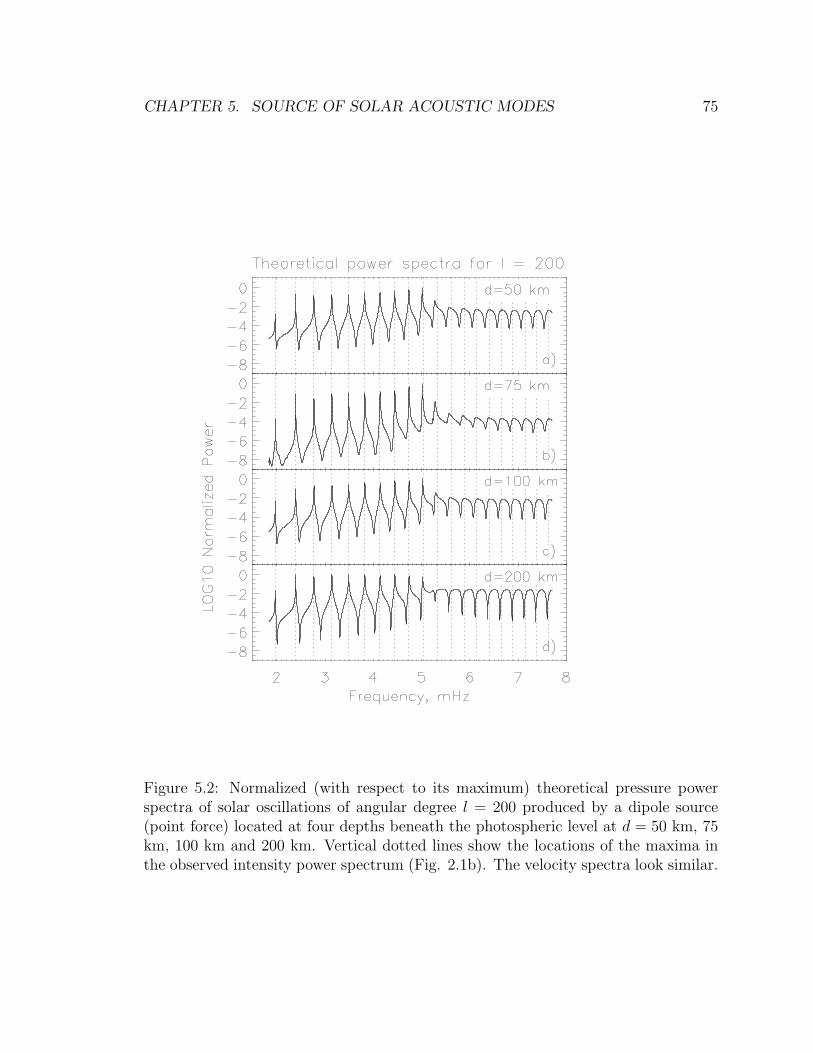
CHAPTER 5. SOURCE OF SOLAR ACOUSTIC MODES 75
Figure 5.2: Normalized (with respect to its maximum) theoretical pressure powerspectra of solar oscillations of angular degree l = 200 produced by a dipole source(point force) located at four depths beneath the photospheric level at d = 50 km, 75km, 100 km and 200 km. Vertical dotted lines show the locations of the maxima inthe observed intensity power spectrum (Fig. 2.1b). The velocity spectra look similar.
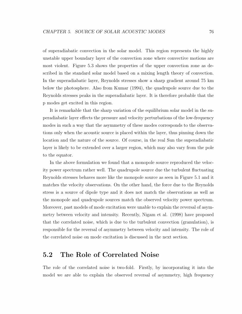
CHAPTER 5. SOURCE OF SOLAR ACOUSTIC MODES 76
of superadiabatic convection in the solar model. This region represents the highly
unstable upper boundary layer of the convection zone where convective motions are
most violent. Figure 5.3 shows the properties of the upper convection zone as de-
scribed in the standard solar model based on a mixing length theory of convection.
In the superadiabatic layer, Reynolds stresses show a sharp gradient around 75 km
below the photosphere. Also from Kumar (1994), the quadrupole source due to the
Reynolds stresses peaks in the superadiabatic layer. It is therefore probable that the
p modes get excited in this region.
It is remarkable that the sharp variation of the equilibrium solar model in the su-
peradiabatic layer effects the pressure and velocity perturbations of the low-frequency
modes in such a way that the asymmetry of these modes corresponds to the observa-
tions only when the acoustic source is placed within the layer, thus pinning down the
location and the nature of the source. Of course, in the real Sun the superadiabatic
layer is likely to be extended over a larger region, which may also vary from the pole
to the equator.
In the above formulation we found that a monopole source reproduced the veloc-
ity power spectrum rather well. The quadrupole source due the turbulent fluctuating
Reynolds stresses behaves more like the monopole source as seen in Figure 5.1 and it
matches the velocity observations. On the other hand, the force due to the Reynolds
stress is a source of dipole type and it does not match the observations as well as
the monopole and quadrupole sources match the observed velocity power spectrum.
Moreover, past models of mode excitation were unable to explain the reversal of asym-
metry between velocity and intensity. Recently, Nigam et al. (1998) have proposed
that the correlated noise, which is due to the turbulent convection (granulation), is
responsible for the reversal of asymmetry between velocity and intensity. The role of
the correlated noise on mode excitation is discussed in the next section.
5.2 The Role of Correlated Noise
The role of the correlated noise is two-fold. Firstly, by incorporating it into the
model we are able to explain the observed reversal of asymmetry, high frequency
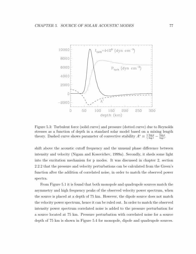
CHAPTER 5. SOURCE OF SOLAR ACOUSTIC MODES 77
Figure 5.3: Turbulent force (solid curve) and pressure (dotted curve) due to Reynoldsstresses as a function of depth in a standard solar model based on a mixing lengththeory. Dashed curve shows parameter of convective stability A∗ ≡ 1
γlog plog r
− log ρlog r
.
shift above the acoustic cutoff frequency and the unusual phase difference between
intensity and velocity (Nigam and Kosovichev, 1999a). Secondly, it sheds some light
into the excitation mechanism for p modes. It was discussed in chapter 2, section
2.2.2 that the pressure and velocity perturbations can be calculated from the Green’s
function after the addition of correlated noise, in order to match the observed power
spectra.
From Figure 5.1 it is found that both monopole and quadrupole sources match the
asymmetry and high frequency peaks of the observed velocity power spectrum, when
the source is placed at a depth of 75 km. However, the dipole source does not match
the velocity power spectrum, hence it can be ruled out. In order to match the observed
intensity power spectrum correlated noise is added to the pressure perturbation for
a source located at 75 km. Pressure perturbation with correlated noise for a source
depth of 75 km is shown in Figure 5.4 for monopole, dipole and quadrupole sources.
CHAPTER 5. SOURCE OF SOLAR ACOUSTIC MODES 78
Figure 5.4: Normalized (with respect to its maximum) theoretical pressure powerspectra of solar oscillations of angular degree l = 200 produced by a source locatedat a depth of 75 km beneath the photospheric level. Three different types of sourcesare considered, to which real correlated noise is added. a) Monopole, relative level ofcorrelated noise = −0.02, (b) Dipole, relative level = −4.0×10⁻⁵ and (c) Quadrupole,relative level = −0.03. These values have been normalized by the maximum valueof the real part of the pressure perturbation. There is no uncorrelated noise in theabove cases. We have applied a threshold (at 10−6) to remove the numerical noise.
CHAPTER 5. SOURCE OF SOLAR ACOUSTIC MODES 79
For different types of sources the level of the correlated noise was adjusted to get
the best possible agreement with the data. The sources happen to be negatively
correlated as also shown by Nigam and Kosovichev (1999a). This is consistent to
the photospheric darkening in the intensity fluctuations prior to the acoustic event as
observed by Goode et al. (1998) and seen in the simulations of Stein and Nordlund
(1998). By adding correlated noise we are able to match the intensity data best with
the help of a monopole source, as compared to the other source types. We are also
able to reverse the asymmetry for the dipole and quadrupole sources too, but they do
not match the asymmetry and high frequency peaks in the observed intensity power
spectrum as well as the monopole source.
The source of the oscillations were located by Goode et al. (1992) close to where
we find in the present paper. They used models and data about the height variation
of the velocity signal in the photosphere to pin down the depth of the source. Also,
Goode et al. (1998) showed a linear dependence on the local convective velocity of the
magnitude of the local excitation of oscillations implying a monopole source, which
is consistent with our finding.
5.3 Summary
Simulating the MDI observations of medium angular degree we find that a source
is located at a depth of 75 ± 50 km below the photosphere, in the superadiabatic
layer. The source appears to be of composite form, consisting of monopole and
quadrupole types. A monopole source provides a best match with the observations in
comparison to the quadrupole source; hence, it may be the dominant term exciting
the p modes. Studying the interaction of the correlated noise with the p modes one
finds that the noise is negatively correlated to the source, which leads to photospheric
darkening prior to the acoustic emission. Therefore, it is possible that the solar p
modes are excited by a combination of mass or entropy fluctuations due to radiative
cooling at the solar surface, which constitute a monopole source and quadrupolar
Reynolds stresses. Studying the phase relation between the correlated noise and the
perturbations could provide an insight into the physics of excitation of solar p modes.
Chapter 6
Conclusions
In this thesis I have discussed the excitation of solar p modes. The main contributions
to the field are an explanation for the reversal in asymmetry between velocity and
intensity power spectra. This then led to the derivation of an asymmetrical fitting
formula to determine the eigenfrequencies of oscillation by fitting both the velocity
and intensity power spectra. I also gave an explanation for the observed phase differ-
ence between velocity and intensity helioseismic spectra. To explain these observed
characteristics a model of excitation for solar p modes is proposed.
The cause of the reversal of asymmetry and the observed phase difference is due
to the presence of correlated noise in the oscillation spectra. This noise happens to
be higher in the intensity observations and can perhaps be attributed to the granu-
lation (Nigam et al., 1998). Solar p modes are believed to be excited by turbulent
convection in the superadiabatic layer, by a combination of mass or entropy fluctua-
tions, which constitute a monopole source and quadrupolar Reynolds stresses (Nigam
and Kosovichev, 1999b). The excitation of p modes could proceed in the following
way: Radiative cooling at the solar surface results in monopolar emission of sound
due to entropy fluctuations, followed by convective downdrafts in the dark narrow
intergrannular lanes. Such mass fluctuations are linked to changes in volume, which
in a gravitationally stratified medium such as the Sun produce dipolar emission via
buoyant acceleration in the cool intergrannular lanes. Finally, the Reynolds stresses
resulting from horizontal flow into the evacuated region left behind by the downflow
80

CHAPTER 6. CONCLUSIONS 81
are responsible for quadrupolar acoustic emission. In the observations of Goode et al.
(1998) and simulations of Nordlund (1985), Stein and Nordlund (1989) the strength
of the acoustic event is correlated to the photospheric darkening that is observed prior
to the occurrence of the event. This supports the notion of the correlated noise that
is introduced in the thesis. Several groups have verified our findings independently
(Kumar and Basu, 1999); (Rast, 1999) . The phase difference between velocity and
intensity that was studied in chapter 3 has been recently confirmed by Oliviero et
al. (1999) and Straus et al. (1999), who attribute the unusual behavior of the phase
to the correlated background. Moreover, the asymmetrical fitting formula is now
being used by the helioseismology community to determine the eigenfrequencies of
oscillation of the solar p and f modes (Antia and Basu, 1999); (Thiery et al., 1999);
(Bertello et al., 1999).
6.1 Directions for Future Work
It would be interesting to verify the above results using numerical simulations of
Stein and Nordlund. The reversal of asymmetry in the intensity power spectra could
then be explained by solving the equations that include radiative transfer in the
optically thin outer layers. Using the model proposed here and the observations
from the different instruments (MDI, GOLF and VIRGO) onboard SOHO, it should
be possible to estimate the correlated noise and study its physics. This would be
very useful in understanding the interaction of oscillations with turbulence. Also
changes in asymmetry and phase difference with solar cycle would be worth studying.
This would be useful in studying the effect that the magnetic field has on the p
mode frequencies. It would be challenging to fit the splittings and take rotation into
account. Ridge fitting could be done using this formula. It would be interesting to see
if the whole spectrum could be fit all at once. Since the correlated noise is much less in
the velocity spectrum compared to the intensity, whether fitting the velocity power
spectrum to determine the eigenfrequencies sufficient? These are a few important
related problems to keep the helioseismologists occupied into the next century.
CHAPTER 6. CONCLUSIONS 82
The effect of asymmetry on the frequencies of p modes will be important in cor-
recting the solar models, in order to match the corrected observed frequencies. This
would in turn have an impact on the celebrated solar neutrino problem (Bahcall and
Davis, 1976).
High spatial and temporal resolution observations would be useful to resolve in-
dividual acoustic sources and study their distribution. This would be invaluable in
studying the physics of excitation of solar p modes. A few years back Brown (1991)
has proposed that these sources are likely to be localized and discrete. Therefore, a
technique using wavelets (Milford and Nigam, 1995) could be applied to the data in
order to study these acoustic events.
A similar study for the f mode could be undertaken. This would then shed light
on its excitation.
The formalism developed in this thesis can be used to theoretically study the
excitation characteristics of g modes. When, if ever, g modes are detected in the Sun,
they can be used to test the predictions of the theory.
The millennium has seen several interesting discoveries. Solar p modes with a
period of about five minutes (Leighton et al., 1962) were discovered only four decades
ago, and the story of mode excitation has been revisited several times by many
authors. There is a long way to go, but we hope to learn more about these acoustic
modes and the Sun in the next century.

Appendix A
Mode Excitation
A derivation of the equations discussed in chapter 2 is carried out here. In §A.1
the basic equation in terms of the Lagrangian pressure perturbation is derived. In
§A.2 the algorithm for the numerical computation of the Green’s function is outlined.
Finally, in §A.3 and §A.4 the Green’s function and the eigenvalue condition for the
simple potential well problem are calculated analytically.
A.1 Linearized equations in terms of Lagrangian
perturbations
The equations (1.22) and (1.23) are rewritten as
dξ
dr+ A11ξ + A12δp = S1 (A.1)
dδp
dr+ A21ξ + A22δp = S2 (A.2)
where
A11 =2
r− L2g
ω2r2(A.3)
83
APPENDIX A. MODE EXCITATION 84
A12 =
(1− L2c2
ω2r2
)1
ρc2(A.4)
A21 = −gρf
r(A.5)
A22 =L2g
ω2r2(A.6)
where f is defined in equation (1.24)
The equations (A.1) and (A.2) are transformed to (see equations (1.30) and (1.31))
d2Ψ
dr2+ K2Ψ = S (A.7)
where Ψ is proportional to the Lagrangian pressure perturbation δp and K is is given
by equations (1.32) or (1.37)
For p modes this equation is simplified as
K2(r) ≈ ω21 − ω2
+
c2(A.8)
where, ω21 = ω2 + iωΓ, and Γ is the damping coefficient.
The composite source corresponding to the Lagrangian pressure perturbation is
S(r, ω) =
[c1
dS2
dr+ c2S2
]+
[c3
dS1
dr+ c4S1
], (A.9)
where c1, c2, c3 and c4 depend on the solar model and are given by:
c1 = 1/u (A.10)
where u is defined by equation
c2 = z/u (A.11)
and z is given by
z = A11 − A′21
A21
= A11 − d(ln A21)
dr(A.12)
APPENDIX A. MODE EXCITATION 85
c3 = −ρg
u(A.13)
c4 = −[zρg + A21 + d(ρg)
dr
]
u(A.14)
A.2 Numerical solution to the Green’s function
The defining equation for the Green’s function is
d2Ψ
dr2+
ω21 − ω2
+
c2Ψ = δ(r − rs), (A.15)
where, ω21 = ω2 + iωΓ
The above equation is discretized using a non-uniform mesh, by finited differ-
ence approximation of the derivative. The following notation is used Ψj = Ψ(rj),
cj = c(rj) and for other variables. The radial variable r has been discretized as
r1, r2, . . . rj, . . . rN.
This is subject to the following boundary conditions: At r = 0
Ψ = 0 (A.16)
At r = R, the radiation condition is applied to ensure outgoing waves. A harmonic
time dependence of eiωt is used.
dΨ
dr+ ikRΨ = 0 (A.17)
where,
k2(r) =ω2
1 − ω2+(r)
c2(r)(A.18)
Evaluating equation (A.18) at r = R leads to

APPENDIX A. MODE EXCITATION 86
k2R = k2(R) =
ω21 − ω2
+R
c2R
(A.19)
If on the other hand a harmonic time dependence of e−iωt is used instead, the
radiation condition is modified to
dΨ
dr− ikRΨ = 0 (A.20)
At the source location r = rs, the solution is continuous, but there is a jump in
the first derivative. There are two solutions Ψ< for 0 < r < rs and Ψ> for rs < r < R.
They are matched at r = rs.
The problem of computing the Green’s function can be formulated as solving the
following differential equations subject to the boundary and matching conditions.
d2Ψ<
dr2+
ω21 − ω2
+
c2Ψ< = 0 (A.21)
d2Ψ>
dr2+
ω21 − ω2
+
c2Ψ> = 0 (A.22)
Ψ<(r) = 0, at r = 0 (A.23)
Ψ<(rs) = Ψ>(rs) (A.24)
dΨ>
dr− dΨ<
dr= 1, at r = rs (A.25)
dΨ>
dr+ ikRΨ> = 0, at r = R (A.26)
The first derivatives are approximated by the following backward difference ap-
proximation
dΨ
dr≈ Ψj −Ψj−1
hj−1
(A.27)
APPENDIX A. MODE EXCITATION 87
and the following forward difference approximation
dΨ
dr≈ Ψj+1 −Ψj
hj
(A.28)
where, hj−1 is the mesh spacing
hj−1 = rj − rj−1 (A.29)
The second derivative is approximated as
d2Ψ
dr2≈ Ψj+1
havgjhj
− 2Ψj
hj−1hj
+Ψj−1
hj−1havgj
(A.30)
where,
havgj=
hj + hj−1
2(A.31)
The differential equations, the boundary and matching conditions can be dis-
cretized using finite differences. They are then combined and this leads to a tridiag-
onal system of equations.
ajΨj−1 + bjΨj + EjΨj+1 = 0 (A.32)
where j = 1,2, . . . p-1,p+1, . . . ,N-1 and, the boundary condition Ψ0 = 0 is used in
the equation (A.32).
At the source position r = rs, j = s
wsΨs−1 + vsΨs + usΨs+1 = 1 (A.33)
At j = N, the radiation condition is applied
βNΨN−1 + αNΨN = 0 (A.34)
where,
APPENDIX A. MODE EXCITATION 88
aj =1
hj−1havgj
(A.35)
bj = k2j − Fj (A.36)
Fj =2
hj−1hj
(A.37)
Ej =1
hjhavgj
(A.38)
ws =1
hs−1
(A.39)
us =1
hs
(A.40)
vs = −(us + ws) (A.41)
βN = − 1
hN−1
(A.42)
αN = −βN + ikN (A.43)
Equations (A.32), (A.33) & (A.34) can be rewritten as a matrix equation
AωXΨ = bs (A.44)
Where Aω is a N X N tridiagonal matrix. XΨ = (Ψ1, . . . , ΨN)T is the unknown
Green’s function that needs to be computed by solving equation (A.44) for each
frequency ω. The right hand side vector bs = (0, . . . , 1, . . . , 0)T , contains a 1 at
location j = s in the array corresponding to the source location r = rs.
APPENDIX A. MODE EXCITATION 89
Aω =
b1 E1 0 0 0 0 . . . 0
a2 b2 E2 0 0 0 . . . 0
0 a3 b3 E3 0 0 . . . 0...
.... . . . . . . . .
......
... 0 0 ws vs us . . . 0
......
......
. . . . . . . . ....
0 . . . 0 0 0 aN−1 bN−1 EN−1
0 . . . 0 0 0 0 βN αN
(A.45)
A.3 Green’s function for the potential well
From chapter 2, equation (2.4) we have
d2Ψ
dr2+
ω21 − V (r)
c2Ψ = δ(r − rs) (A.46)
where Ψ is proportional to the pressure perturbation.
ω21 = (ω2 + iωΓ) (A.47)
The source is placed inside the well, 0 < rs < a. Without loss of generality
consider frequencies ω < ωc. The solution Ψ = 0 at r = 0 and the radiation condition
is applied far away from the upper turning point r = a. This ensures propagating
waves for frequencies ω > ωc and exponential decay for waves with ω < ωc.
The above equation with the boundary conditions needs to be solved in the three
regions:
i) 0 ≤ r < rs: satisfied by Ψ1, with Ψ1 = 0 at r = 0.
ii) rs < r < a: satisfied by Ψ2.
iii) r ≥ a: satisfied by an exponentially decaying solution Ψ3.
These three solutions satisfy three different differential equations in each of the three
regions.
d2Ψ1
dr2+ W 2
1 Ψ1 = 0 (A.48)

APPENDIX A. MODE EXCITATION 90
d2Ψ2
dr2+ W 2
1 Ψ2 = 0 (A.49)
d2Ψ3
dr2−W 2
2 Ψ2 = 0 (A.50)
where,
W1 =ω1
c(A.51)
W2 =ω2
c(A.52)
ω22 = (ω2
c − ω21) (A.53)
The solutions to the differential equations with the boundary conditions are:
Ψ1(r) = c1 sin(W1r) (A.54)
Ψ2(r) = c2 sin(W1r) + c3 cos(W1r) (A.55)
Ψ3(r) = c4e−W2r (A.56)
The constants c1, c2, c3 and c4 are obtained by applying matching conditions at r = rs
and r = a.
At r = rs due to the delta function, the solution is continuous, but there is a jump
in the first derivative.
Ψ1(rs) = Ψ2(rs) (A.57)
dΨ2
dr− dΨ1
dr= 1, at r = rs (A.58)
APPENDIX A. MODE EXCITATION 91
At r = a, both the function and its first derivative are continuous.
Ψ2(a) = Ψ3(a) (A.59)
dΨ2
dr=
dΨ3
dr, at r = a (A.60)
Applying these matching conditions and carrying out the algebra, the constant c4 is
c4 = − sin(W1rs)
W1 cos(W1a) + W2 sin(W1a)eW2a (A.61)
The Green’s function at r ≥ a is GΨ(r, rs) = Ψ3(r) = c4e−W2r
GΨ(r, rs) =−c sin(ω1rs/c)
ω1cos(ω1a/c) + ω2sin(ω1a/c)e−ω2(r−a)/c (A.62)
For frequencies ω > ωc, ω2 becomes imaginary. Replacing ω2 by ik in the above
expression (A.62), we get the corresponding Green’s function. Where k is
k2 = (ω21 − ω2
c ) (A.63)
A.4 Eigenfrequencies for the potential well
The governing equation for the eigenfrequency ω0 is
d2Ψ
dr2+
ω20 − V (r)
c2Ψ = 0 (A.64)
where Ψ is proportional to the pressure perturbation.
Without loss of generality consider eigenfrequencies ω0 < ωc. The solution Ψ = 0
at r = 0 and the radiation condition is applied far away from the upper turning point
r = a. This ensures propagating waves for eigenfrequencies ω0 > ωc and exponential
decay for waves with ω0 < ωc.
The above equation (A.64) with the boundary conditions needs to be solved in
the two regions:
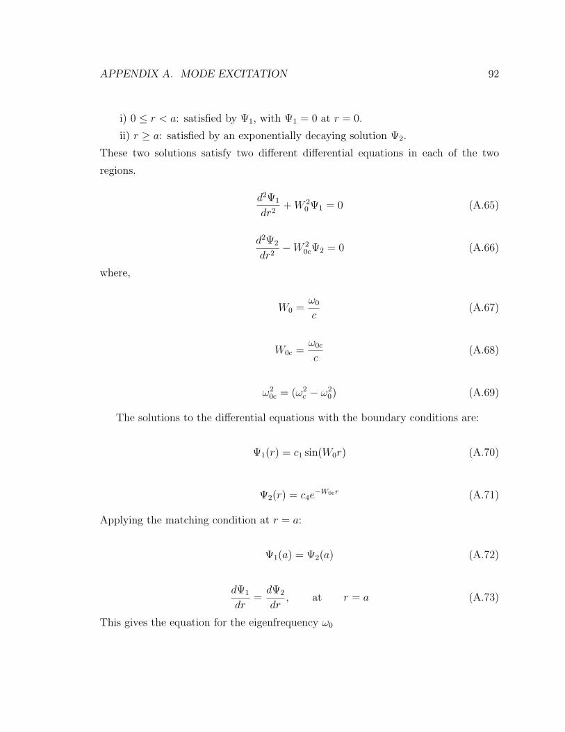
APPENDIX A. MODE EXCITATION 92
i) 0 ≤ r < a: satisfied by Ψ1, with Ψ1 = 0 at r = 0.
ii) r ≥ a: satisfied by an exponentially decaying solution Ψ2.
These two solutions satisfy two different differential equations in each of the two
regions.
d2Ψ1
dr2+ W 2
0 Ψ1 = 0 (A.65)
d2Ψ2
dr2−W 2
0cΨ2 = 0 (A.66)
where,
W0 =ω0
c(A.67)
W0c =ω0c
c(A.68)
ω20c = (ω2
c − ω20) (A.69)
The solutions to the differential equations with the boundary conditions are:
Ψ1(r) = c1 sin(W0r) (A.70)
Ψ2(r) = c4e−W0cr (A.71)
Applying the matching condition at r = a:
Ψ1(a) = Ψ2(a) (A.72)
dΨ1
dr=
dΨ2
dr, at r = a (A.73)
This gives the equation for the eigenfrequency ω0

APPENDIX A. MODE EXCITATION 93
ω0c sin(W0a) + W0 cos(W0a) = 0 (A.74)
The equation (A.74) also holds for eigenfrequencies ω0 > ωc, in which case ω0c becomes
imaginary.

Appendix B
Phase and Amplitude differences
In this appendix the equations used in chapter 3 are derived.
The Green’s function is given by (from equation (A.62))
GΨ(ω1) =−c sin(ω1rs/c)
ω1cos(ω1a/c) + ω2sin(ω1a/c)e−ω2(r−a)/c (B.1)
where ω1 and ω2 are given by:
ω21 = (ω2 + iωΓ) (B.2)
ω22 = (ω2
c − ω21) (B.3)
For solar p modes the damping coefficient Γ ¿ ω, using the binomial expansion,
equation (B.2) becomes
ω1 = ω + iΓ/2 (B.4)
The denominator D of equation (B.1) is
D = ω1 cos(ω1a/c) + ω2 sin(ω1a/c) (B.5)
The above equation (B.5) can be rewritten as
D = ωc sin(ω1a/c + φc) (B.6)
94

APPENDIX B. PHASE AND AMPLITUDE DIFFERENCES 95
where
sin φc =ω1
ωc
≈ ω
ωc
(B.7)
From equation (1.29) δp = uΨ and since the Green’s function is proportional to
Ψ, therefore δp ∝ GΨ. Taking into account the time dependence eiωt, for modes below
the acoustic cutoff frequency ωc
δp ∝ −αc
ωc
eiωte−ωc(r−a)/c (B.8)
where α is a complex analytical function of ω, a, rs, c and the damping, and is given
by
α =sin(ω1rs/c)
sin(ω1a/c + φc)(B.9)
Using the equation of continuity, and the adiabatic relation,
dδρ
dt+ ρ
dδv
dr= 0 (B.10)
δρ =δp
c2(B.11)
the velocity perturbation is given by
δv =δp ω
cρωc
eiπ/2 (B.12)
where ρ is the density which has been assumed to be constant in this simple model.
Without loss of generality both the pressure and velocity perturbations can be eval-
uated at the upper turning point r = a.
The cross spectrum Sxy between two complex numbers x = rxeiθx and y = rye
iθy
is defined as
Sxy = xy∗ = rxryei(θx−θy) (B.13)
The modulus of Sxy is rxry and its phase is θx − θy.
The power contrast of the power of quantity ψ (p or v), Pψ, relative to the power

APPENDIX B. PHASE AND AMPLITUDE DIFFERENCES 96
of the uncorrelated background Pψ,uncor, is Cψ and is given by
Cψ =(δψ + Nψ,cor)(δψ + Nψ,cor)
∗
Pψ,uncor
(B.14)
where ψ can be p or v, and Cψ = Pψ/Pψ,uncor.
Cψ =|δψ|2
Pψ,uncor
+ βψ
[1 +
δψN∗ψ,cor + δψ∗Nψ,cor
|Nψ,cor|2]
(B.15)
where βψ = |Nψ,cor|2/Pψ,uncor is the ratio of the power of correlated, |Nψ,cor|2, to
uncorrelated noise.
The above equation (B.15) can be rewritten, using the fact |Nψ,cor|2 = Nψ,corN∗ψ,cor,
as
Cψ =|δψ|2
Pψ,uncor
+ βψ
[1 +
(δψ
Nψ,cor
+δψ∗
N∗ψ,cor
)](B.16)
Further, by considering that
δψ
Nψ,cor
+δψ∗
N∗ψ,cor
= 2Re
(δψ
Nψ,cor
)(B.17)
The expression of the power contrast in equation (B.16) is then (see also Eq. (3.9))
Cψ =|δψ|2
Pψ,uncor
+ βψ
[1 + 2Re
(δψ
Nψ,cor
)](B.18)

Appendix C
Fitting formula
Derivations of the various equations in chapter 4 of the thesis are carried out here.
In §C.1 the asymmetrical fitting formula is derived. In §C.2 the basic idea of fitting
is explained. Finally, in §C.3 the eigenfrequencies of the solar model are computed
numerically, for both reflecting and radiation boundary conditions.
C.1 Derivation of the fitting formula
The Green’s function is
GΨ(ω1) =−c sin(ω1rs/c)
ω1cos(ω1a/c) + ω2sin(ω1a/c)e−ω2(r−a)/c (C.1)
where ω1 and ω2 are given by:
ω21 = (ω2 + iωΓ) (C.2)
ω22 = (ω2
c − ω21) (C.3)
For solar p modes the damping coefficient Γ ¿ ω, using the binomial expansion
equation (C.2) becomes
ω1 = ω + iΓ/2 (C.4)
97
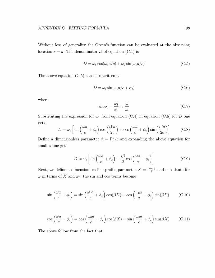
APPENDIX C. FITTING FORMULA 98
Without loss of generality the Green’s function can be evaluated at the observing
location r = a. The denominator D of equation (C.1) is
D = ω1 cos(ω1a/c) + ω2 sin(ω1a/c) (C.5)
The above equation (C.5) can be rewritten as
D = ωc sin(ω1a/c + φc) (C.6)
where
sin φc =ω1
ωc
≈ ω
ωc
(C.7)
Substituting the expression for ω1 from equation (C.4) in equation (C.6) for D one
gets
D = ωc
[sin
(ωa
c+ φc
)cos
(iΓa
2c
)+ cos
(ωa
c+ φc
)sin
(iΓa
2c
)](C.8)
Define a dimensionless parameter β = Γa/c and expanding the above equation for
small β one gets
D ≈ ωc
[sin
(ωa
c+ φc
)+
iβ
2cos
(ωa
c+ φc
)](C.9)
Next, we define a dimensionless line profile parameter X = ω−ω0
Γand substitute for
ω in terms of X and ω0, the sin and cos terms become
sin(
ωa
c+ φc
)= sin
(ω0a
c+ φc
)cos(βX) + cos
(ω0a
c+ φc
)sin(βX) (C.10)
cos(
ωa
c+ φc
)= cos
(ω0a
c+ φc
)cos(βX)− sin
(ω0a
c+ φc
)sin(βX) (C.11)
The above follow from the fact that
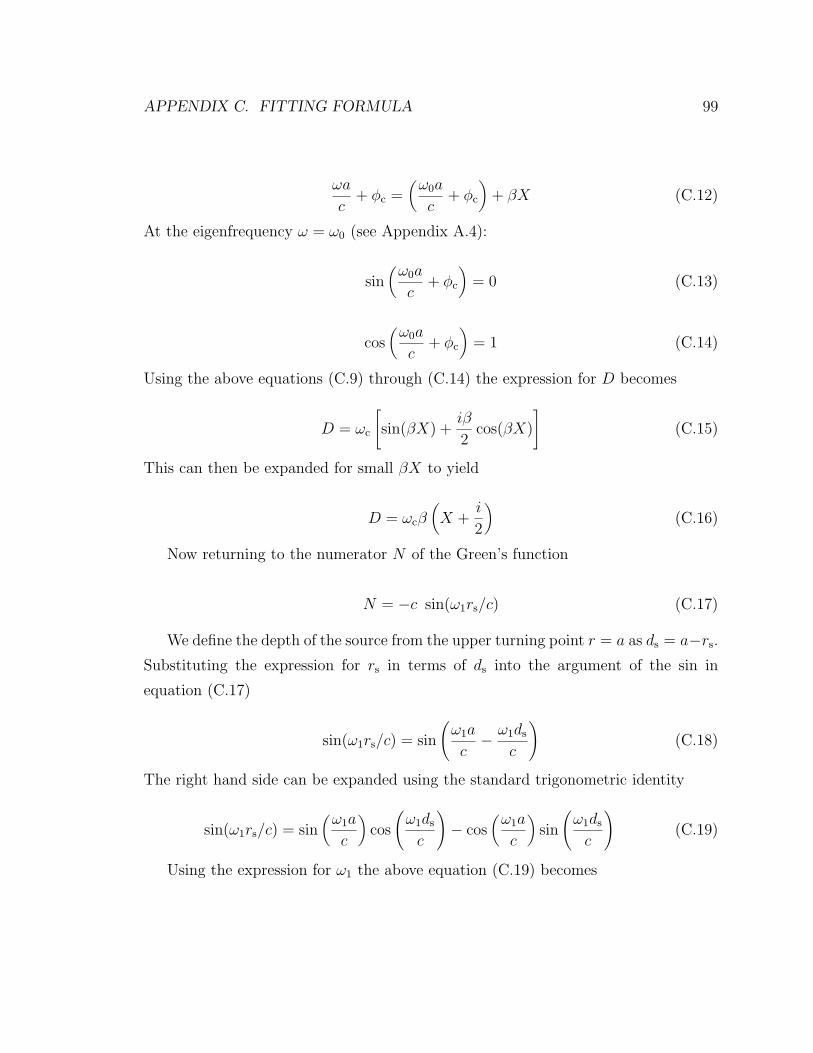
APPENDIX C. FITTING FORMULA 99
ωa
c+ φc =
(ω0a
c+ φc
)+ βX (C.12)
At the eigenfrequency ω = ω0 (see Appendix A.4):
sin(
ω0a
c+ φc
)= 0 (C.13)
cos(
ω0a
c+ φc
)= 1 (C.14)
Using the above equations (C.9) through (C.14) the expression for D becomes
D = ωc
[sin(βX) +
iβ
2cos(βX)
](C.15)
This can then be expanded for small βX to yield
D = ωcβ(X +
i
2
)(C.16)
Now returning to the numerator N of the Green’s function
N = −c sin(ω1rs/c) (C.17)
We define the depth of the source from the upper turning point r = a as ds = a−rs.
Substituting the expression for rs in terms of ds into the argument of the sin in
equation (C.17)
sin(ω1rs/c) = sin
(ω1a
c− ω1ds
c
)(C.18)
The right hand side can be expanded using the standard trigonometric identity
sin(ω1rs/c) = sin(
ω1a
c
)cos
(ω1ds
c
)− cos
(ω1a
c
)sin
(ω1ds
c
)(C.19)
Using the expression for ω1 the above equation (C.19) becomes

APPENDIX C. FITTING FORMULA 100
sin(ω1rs/c) = sin
(ωa
c+
iβ
2
)cos
(ωds
c+
iΓds
2c
)− cos
(ωa
c+
iβ
2
)sin
(ωds
c+
iΓds
2c
)
(C.20)
The above equation (C.20) can be simplified for small β and Γds
c
S ≈[sin
(ωa
c
)+
iβ
2cos
(ωa
c
)]cos
(ωds
c
)−
[cos
(ωa
c
)− iβ
2sin
(ωa
c
)]sin
(ωds
c
)
(C.21)
Where we have used the fact that cos(y) ≈ 1 and sin(y) ≈ y for small y and S =
sin(ω1rs/c). Substituting ω = ω0 + XΓ into the above equation (C.21) and using the
eigenvalue condition ω0ac
= nπ − φc, where n = 0, 1, ... Without loss of generality
consider n = 0. With this substitution and approximating for small Γds
cthe equation
(C.21) becomes
S ≈[sin(βX − φc) +
iβ
2cos(βX − φc)
]cos p0−
[cos(βX − φc)− iβ
2sin(βX − φc)
]sin p0
(C.22)
where p0 = ω0ds
c. The above equation (C.22) can be simplified to
S = sin(βX − pw) +iβ
2cos(βX − pw) (C.23)
where pw = p0 + φc.
The Green’s function then becomes
GΨ ≈−c
[sin(βX − pw) + iβ
2cos(βX − pw)
]
ωc
[sin(βX) + iβ
2cos(βX)
] (C.24)
We get the complex amplitude of the pressure perturbation AΨ from the Green’s
function
AΨ(X) = −Aw
sin(βX − pw) + i2β cos(βX − pw)
sin(βX) + i2β cos(βX)
(C.25)
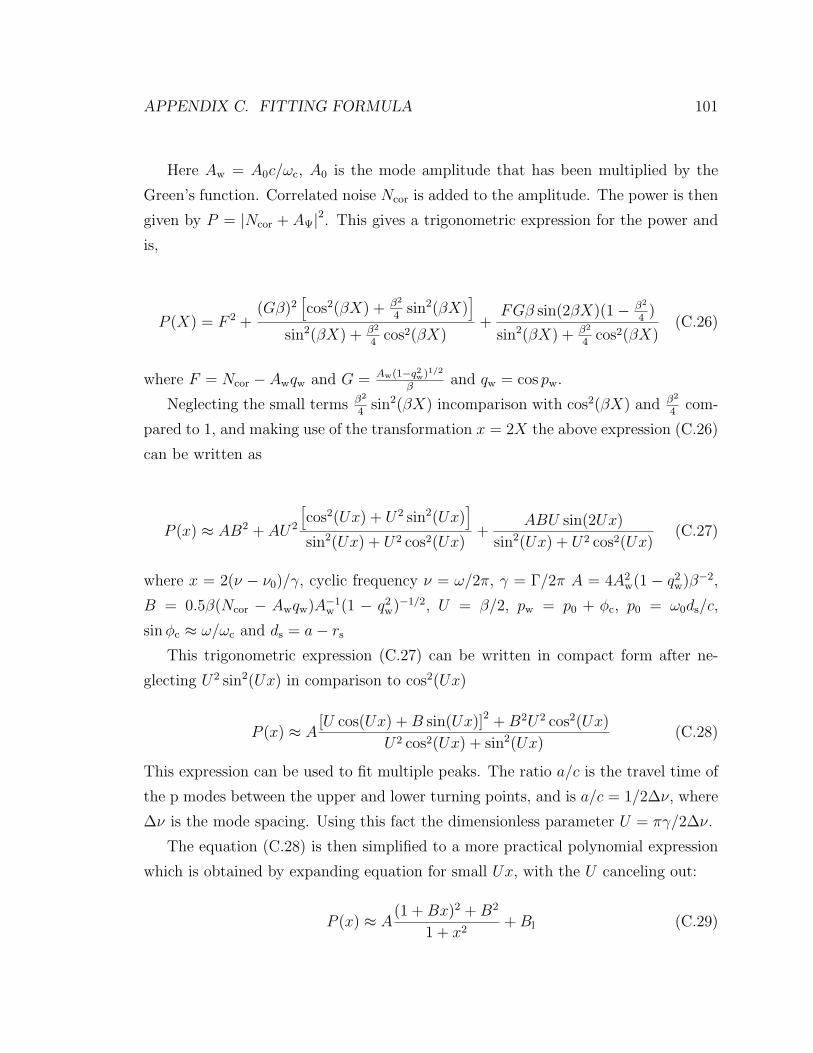
APPENDIX C. FITTING FORMULA 101
Here Aw = A0c/ωc, A0 is the mode amplitude that has been multiplied by the
Green’s function. Correlated noise Ncor is added to the amplitude. The power is then
given by P = |Ncor + AΨ|2. This gives a trigonometric expression for the power and
is,
P (X) = F 2 +(Gβ)2
[cos2(βX) + β2
4sin2(βX)
]
sin2(βX) + β2
4cos2(βX)
+FGβ sin(2βX)(1− β2
4)
sin2(βX) + β2
4cos2(βX)
(C.26)
where F = Ncor − Awqw and G = Aw(1−q2w)1/2
βand qw = cos pw.
Neglecting the small terms β2
4sin2(βX) incomparison with cos2(βX) and β2
4com-
pared to 1, and making use of the transformation x = 2X the above expression (C.26)
can be written as
P (x) ≈ AB2 + AU2
[cos2(Ux) + U2 sin2(Ux)
]
sin2(Ux) + U2 cos2(Ux)+
ABU sin(2Ux)
sin2(Ux) + U2 cos2(Ux)(C.27)
where x = 2(ν − ν0)/γ, cyclic frequency ν = ω/2π, γ = Γ/2π A = 4A2w(1 − q2
w)β−2,
B = 0.5β(Ncor − Awqw)A−1w (1 − q2
w)−1/2, U = β/2, pw = p0 + φc, p0 = ω0ds/c,
sin φc ≈ ω/ωc and ds = a− rs
This trigonometric expression (C.27) can be written in compact form after ne-
glecting U2 sin2(Ux) in comparison to cos2(Ux)
P (x) ≈ A[U cos(Ux) + B sin(Ux)]2 + B2U2 cos2(Ux)
U2 cos2(Ux) + sin2(Ux)(C.28)
This expression can be used to fit multiple peaks. The ratio a/c is the travel time of
the p modes between the upper and lower turning points, and is a/c = 1/2∆ν, where
∆ν is the mode spacing. Using this fact the dimensionless parameter U = πγ/2∆ν.
The equation (C.28) is then simplified to a more practical polynomial expression
which is obtained by expanding equation for small Ux, with the U canceling out:
P (x) ≈ A(1 + Bx)2 + B2
1 + x2+ Bl (C.29)

APPENDIX C. FITTING FORMULA 102
To this one can add the linear uncorrelated background Bl = c1+c2ν, where c1 and c2
are fitting parameters, which results in equation (4.4) in chapter 4 of the main text.
C.2 Fitting power spectra by the formula
Given a target power spectrum Pt(ν), fitting is carried out by minimizing the square
of the difference between the power estimated by the above formula P (ν) and Pt(ν),
summed over a suitable range so as to isolate the mode.
∆ =N∑
j=1
[Pt(νj)− P (νj)]2 (C.30)
where, ν1, ν2, . . . , νN are the N frequency mesh points.
The nonlinear minimization of ∆ is done with respect to a set of six parameters
S = A,B, γ, ν0, c1, c2 using Powell’s algorithm from the IDL library.
minS
∆ (C.31)
C.3 Numerical solution of the eigenvalue problem
C.3.1 Reflecting boundary conditions
The eigenfrequencies ω0 of the solar model are computed from the following equation
d2Ψ
dr2+
ω20 − ω2
+
c2Ψ = 0, (C.32)
For computing just the bound states, reflecting boundary conditions Ψ = 0 at r = 0
and r = R is applied. The above equation (C.32) is discretized using a non-uniform
mesh, by using finite difference approximation to the derivative. The following nota-
tion is used Ψj = Ψ(rj), cj = c(rj) and similarly for the other variables.
The second derivative is approximated as
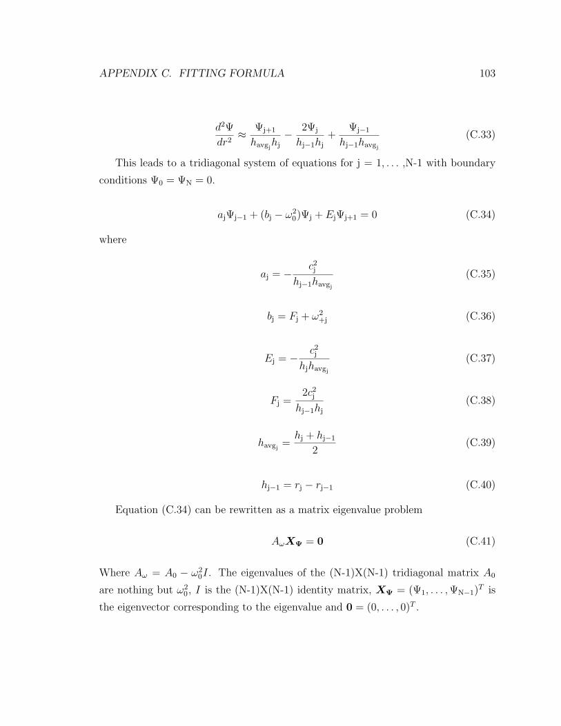
APPENDIX C. FITTING FORMULA 103
d2Ψ
dr2≈ Ψj+1
havgjhj
− 2Ψj
hj−1hj
+Ψj−1
hj−1havgj
(C.33)
This leads to a tridiagonal system of equations for j = 1, . . . ,N-1 with boundary
conditions Ψ0 = ΨN = 0.
ajΨj−1 + (bj − ω20)Ψj + EjΨj+1 = 0 (C.34)
where
aj = − c2j
hj−1havgj
(C.35)
bj = Fj + ω2+j (C.36)
Ej = − c2j
hjhavgj
(C.37)
Fj =2c2
j
hj−1hj
(C.38)
havgj=
hj + hj−1
2(C.39)
hj−1 = rj − rj−1 (C.40)
Equation (C.34) can be rewritten as a matrix eigenvalue problem
AωXΨ = 0 (C.41)
Where Aω = A0 − ω20I. The eigenvalues of the (N-1)X(N-1) tridiagonal matrix A0
are nothing but ω20, I is the (N-1)X(N-1) identity matrix, XΨ = (Ψ1, . . . , ΨN−1)
T is
the eigenvector corresponding to the eigenvalue and 0 = (0, . . . , 0)T .
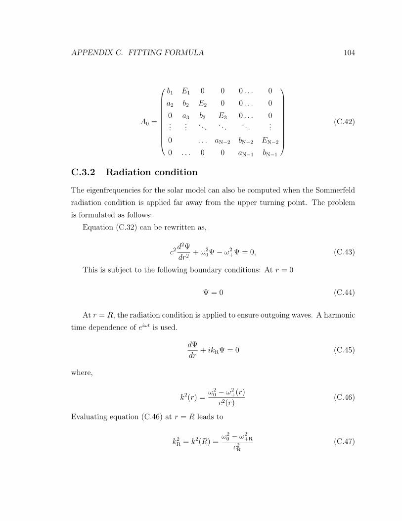
APPENDIX C. FITTING FORMULA 104
A0 =
b1 E1 0 0 0 . . . 0
a2 b2 E2 0 0 . . . 0
0 a3 b3 E3 0 . . . 0...
.... . . . . . . . .
...
0 . . . aN−2 bN−2 EN−2
0 . . . 0 0 aN−1 bN−1
(C.42)
C.3.2 Radiation condition
The eigenfrequencies for the solar model can also be computed when the Sommerfeld
radiation condition is applied far away from the upper turning point. The problem
is formulated as follows:
Equation (C.32) can be rewritten as,
c2d2Ψ
dr2+ ω2
0Ψ− ω2+Ψ = 0, (C.43)
This is subject to the following boundary conditions: At r = 0
Ψ = 0 (C.44)
At r = R, the radiation condition is applied to ensure outgoing waves. A harmonic
time dependence of eiωt is used.
dΨ
dr+ ikRΨ = 0 (C.45)
where,
k2(r) =ω2
0 − ω2+(r)
c2(r)(C.46)
Evaluating equation (C.46) at r = R leads to
k2R = k2(R) =
ω20 − ω2
+R
c2R
(C.47)

APPENDIX C. FITTING FORMULA 105
From equations (C.43) and (C.47) one obtains
c2
c2R
d2Ψ
dr2+
ω2+R − ω2
+
c2R
Ψ + k2RΨ = 0 (C.48)
Defining a new variable Φ = kRΨ, one obtains the following set of equations
c2
c2R
d2Ψ
dr2+
ω2+R − ω2
+
c2R
Ψ + kRΦ = 0 (C.49)
kRΨ− Φ = 0 (C.50)
These equations (C.49) and (C.50) are to be solved subject to the following bound-
ary conditions Ψ = Φ = 0 at r = 0.
At r = R the radiation condition is applied on Ψ and Φ
dΨ
dr+ ikRΨ = 0 (C.51)
dΦ
dr+ ikRΦ = 0 (C.52)
The first derivatives are approximated by the following backward difference approxi-
mation
dΨ
dr≈ Ψj −Ψj−1
hj−1
(C.53)
The boundary conditions and the equations can be discretized by using finite differ-
ences and are
Ψ0 = 0 (C.54)
Φ0 = 0 (C.55)
The following equations are written at the interior mesh points j = 1, . . . ,N-1
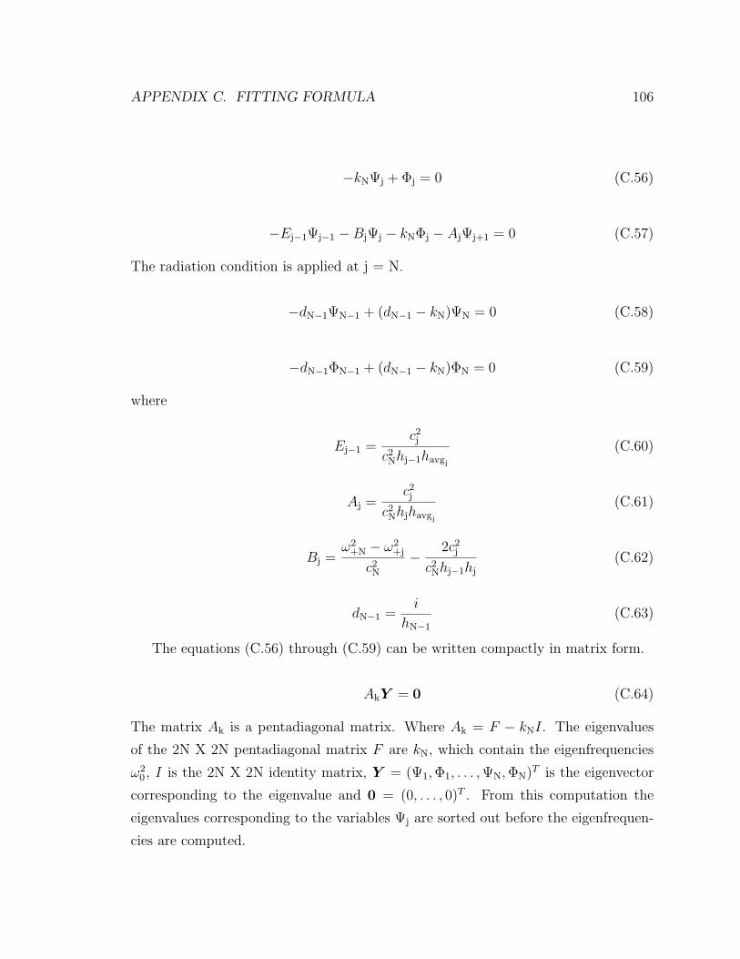
APPENDIX C. FITTING FORMULA 106
−kNΨj + Φj = 0 (C.56)
−Ej−1Ψj−1 −BjΨj − kNΦj − AjΨj+1 = 0 (C.57)
The radiation condition is applied at j = N.
−dN−1ΨN−1 + (dN−1 − kN)ΨN = 0 (C.58)
−dN−1ΦN−1 + (dN−1 − kN)ΦN = 0 (C.59)
where
Ej−1 =c2j
c2Nhj−1havgj
(C.60)
Aj =c2j
c2Nhjhavgj
(C.61)
Bj =ω2
+N − ω2+j
c2N
− 2c2j
c2Nhj−1hj
(C.62)
dN−1 =i
hN−1
(C.63)
The equations (C.56) through (C.59) can be written compactly in matrix form.
AkY = 0 (C.64)
The matrix Ak is a pentadiagonal matrix. Where Ak = F − kNI. The eigenvalues
of the 2N X 2N pentadiagonal matrix F are kN, which contain the eigenfrequencies
ω20, I is the 2N X 2N identity matrix, Y = (Ψ1, Φ1, . . . , ΨN, ΦN)T is the eigenvector
corresponding to the eigenvalue and 0 = (0, . . . , 0)T . From this computation the
eigenvalues corresponding to the variables Ψj are sorted out before the eigenfrequen-
cies are computed.
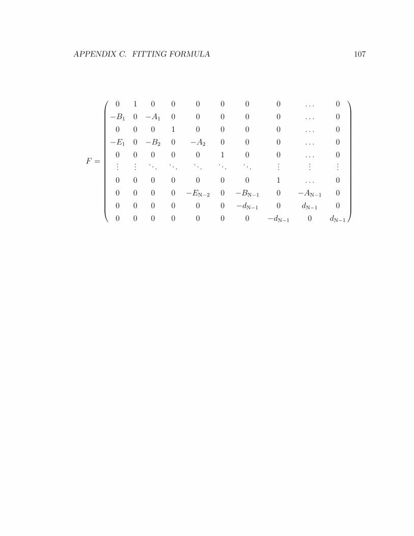
APPENDIX C. FITTING FORMULA 107
F =
0 1 0 0 0 0 0 0 . . . 0
−B1 0 −A1 0 0 0 0 0 . . . 0
0 0 0 1 0 0 0 0 . . . 0
−E1 0 −B2 0 −A2 0 0 0 . . . 0
0 0 0 0 0 1 0 0 . . . 0...
.... . . . . . . . . . . . . . .
......
...
0 0 0 0 0 0 0 1 . . . 0
0 0 0 0 −EN−2 0 −BN−1 0 −AN−1 0
0 0 0 0 0 0 −dN−1 0 dN−1 0
0 0 0 0 0 0 0 −dN−1 0 dN−1
Appendix D
The Source of p modes
The equations relating the excitation of p modes by different source types in Chapter
5 are derived here.
The composite source corresponding to the Lagrangian pressure perturbation is
S(r, ω) =
[c1
dS2
dr+ c2S2
]+
[c3
dS1
dr+ c4S1
], (D.1)
where c1, c2, c3 and c4 depend on the solar model and are given by:
c1 = 1/u (D.2)
where u is defined by equation (1.29)
c2 = z/u (D.3)
and z is given by
z = A11 − A′21
A21
= A11 − d(ln A21)
dr(D.4)
c3 = −ρg
u(D.5)
108
APPENDIX D. THE SOURCE OF P MODES 109
c4 = −[zρg + A21 + d(ρg)
dr
]
u(D.6)
A11 and A21 are given by
A11 =2
r− L2g
ω2r2(D.7)
A21 = −gρf
r(D.8)
where L2 = l(l + 1) and f has been defined by equation (1.24).
The above source can be broken up into monopole Smon, dipole Sdip and quadrupole
Squd sources respectively, which are given by
Smon = c4S1 (D.9)
Sdip−mon = c3dS1
dr(D.10)
where Sdip−mon is the dipole source due to monopole
Sdip = c1dS2
dr+ c2S2 (D.11)
The pressure perturbation δp for these source types can be computed by linear
superposition from the Green’s function.
Ψ(R) =∫ R
0GΨ(r, rs)S(rs)drs (D.12)
where δp(r) = u(r)Ψ(r).
For a monopole source
Ψmon(R) =∫ R
0GΨ(r, rs)c4(rs)S1(rs)drs (D.13)
Considering a single source location rs one gets for a monopole source,
APPENDIX D. THE SOURCE OF P MODES 110
δpmon(robs) ∝ c5(rs)GΨ(robs, rs), (D.14)
where c5(rs) is
c5(rs) = c4(rs)u(robs) (D.15)
For, the dipole source produced by the monopole source Sdip−mon, the pressure
perturbation is proportional to the Green’s function as in equation (D.14) above.
For a dipole source,
Ψdip(R) =∫ R
0GΨ(r, rs)
[c1
dS2
drs
+ c2S2(rs)
]drs (D.16)
The derivative in the S2 term can be transferred to the Green’s function by an inte-
gration by parts
∫ R
0GΨ(r, rs)
dS2
drs
drs = −∫ R
0
dGΨ(r, rs)
drs
S2drs (D.17)
The other term in the integration by parts GΨS2 vanishes at the two limits because
the source S2 is localized and is zero at those limits.
Ψdip(R) =∫ R
0
[c2(rs)GΨ − d (c1(rs)GΨ)
drs
]S2(rs)drs (D.18)
Now, considering a single source location rs one gets for a dipole source,
δpdip(robs) ∝ c6(rs)GΨ − d
drs
(GΨ
c7(rs)
), (D.19)
where c6 and c7 are
c6(rs) = c2(rs)u(robs) (D.20)
c7(rs) =1
c1(rs)u(robs)(D.21)
Finally, consider the quadrupole source Squd

APPENDIX D. THE SOURCE OF P MODES 111
S2 ≈ dSqud
dr(D.22)
where Squd is equal to the Reynolds stress ρvv. Substituting S2 in equation
Ψqud(R) =∫ R
0
([c2(rs)GΨ − d (c1(rs)GΨ)
drs
]dSqud
drs
)drs (D.23)
and carrying out a similar integration by parts as was done for the dipole source one
gets
δpqud(robs) ∝ d2
dr2s
(GΨ
c7(rs)
)− d
drs
(GΨ
c8(rs)
)(D.24)
where c8 = 1/c6
The radial component of the displacement ξ is computed from δp using the equa-
tion below
dδp
dr+
L2g
ω2r2δp− gρf
rξ = 0 (D.25)
The velocity perturbation δv = iωξ is then computed for the different source types.

Bibliography
Abrams, D. and Kumar, P.: 1996, The Astrophysical Journal 472, 882.
Anderson, E. R., Duvall, T. L., and Jefferies, S. M.: 1990, The Astrophysical Journal
364, 699.
Antia, H. M. and Basu, S.: 1999, The Astrophysical Journal 519, 400.
Appourchaux, T., Telljohann, U., Martin, D., Fleur, J., and Leveque, S.: 1995a, in
J. T. Hoeksema, V. Domingo, B. Fleck, and B. Battrick (eds.), Fourth SOHO
Workshop Helioseismology. Proceedings. ESA SP-376, (Paris: ESA) vol.2, 359.
Appourchaux, T., Toutain, T., Gough, D. ., and Kosovichev, A. G.: 1995b, in R. K.
Ulrich, E. J. Rhodes, and W. Dappen (eds.), Helio- And Astero-Seismology from
the Earth and Space, GONG 1994: Astr. Soc. Pac., San Francisco, 76, p. 314-317.
Bahcall, J. N. and Davis, R.: 1976, Science 191, 264.
Balmforth, N. J.: 1992, Monthly Notices Of The Royal Astronomical Society 255,
639.
Bertello, L., Henney, C. J., Ulrich, R. K., Varadi, F., Kosovichev, A. G., Scherrer,
P. H., Roca Cortes, T., Thiery, S., Boumier, P., and Turck-Chieze, S.: 1999, The
Astrophysical Journal, submitted.
Bracewell, R. N.: 1986, The Fourier Transform and its Applications, 2nd ed., Rev.,
McGraw-Hill, New York.
Brown, T. M.: 1991, The Astrophysical Journal 371, 396.
Christensen-Dalsgaard, J.: 1994, Lecture Notes on Stellar Oscillations: Institut for
Fysik og Astronomi, Aarhus Universitet, 3rd ed.
Christensen-Dalsgaard, J., Dappen, W., Ajukov, S. V., Anderson, E. R., Antia, H. M.,
Basu, S., Baturin, V. A., Berthomieu, G., Chaboyer, B., Chitre, S. M., Cox, A. N.,
112
BIBLIOGRAPHY 113
Demarque, P., Donatowicz, J., Dziembowski, W. A., Gabriel, M., Gough, D. O.,
Guenther, D. B., Guzik, J. A., Harvey, J. W., Hill, F., Houdek, G., Iglesias, C. A.,
Kosovichev, A. G., Leibacher, J. W., Morel, P., Proffitt, C. R., Provost, J., Reiter,
J., Rhodes, E. J., Rogers, F. J., Roxburgh, I. W., Thompson, M. J., and Ulrich,
R. K.: 1996, Science 272, 1286.
Crighton, D. G.: 1975, Progress In Aerospace Science 16, 31.
Deubner, F.-L.: 1975, Astronomy and Astrophysics 44, 371.
Deubner, F.-L. and Fleck, B.: 1989, Astronomy and Astrophysics 213, 423.
Deubner, F.-L., Fleck, B., Schmitz, F., and Straus, T.: 1992, Astronomy and Astro-
physics 266, 560.
Duvall, T. L., Jefferies, S. M., Harvey, J. W., Osaki, Y., and Pomerantzi, M. A.:
1993, The Astrophysical Journal 410, 829.
Fossat, E.: 1991, Solar Physics 133, 1.
Frohlich, C., Romero, J., Roth, H., Wehrli, C., Anderson, B. N., Appourchaux, T.,
Domingo, V., Telljohann, U., Berthomieu, G., Delache, P., Provost, J., Toutain,
T., Crommelynck, D. A., Chevalier, A., Fichot, A., Dappen, W., Gough, D. O.,
Hoeksema, T., Jimenez, A., Gomez, M. F., Herreros, J. M., Roca Cortes, T.,
Jones, A. R., Pap, J. M., and Willson, R. C.: 1995, Solar Physics 162, 101.
Frohlich, C., Toutain, T., Bonnet, R. M., Bruns, A. V., Delaboudiniere, J. P.,
Domingo, V., Kotov, V. A., Kollath, Z., Rashkovsky, D. N., Vial, J. C., and
Wehrli, C.: 1990, in G. Berthomieu and M. Cribier (eds.), Inside the Sun, (Dor-
drecht: Kluwer), 279.
Gabriel, M.: 1992, Astronomy and Astrophysics 265, 771.
Gabriel, M.: 1993, Astronomy and Astrophysics 274, 935.
Gabriel, M.: 1995, Astronomy and Astrophysics 299, 245.
Gabriel, M.: 1998, Astronomy and Astrophysics 330, 359.
Goldreich, P. and Keeley, D. A.: 1977, The Astrophysical Journal 212, 243.
Goldreich, P. and Kumar, P.: 1988, The Astrophysical Journal 326, 462.
Goldreich, P. and Kumar, P.: 1990, The Astrophysical Journal 363, 694.
Goldreich, P., Murray, N., and Kumar, P.: 1994, The Astrophysical Journal 424, 466.
Goode, P. R., Gough, D. O., and Kosovichev, A. G.: 1992, The Astrophysical Journal

BIBLIOGRAPHY 114
387, 707.
Goode, P. R., Strous, L. H., Rimmele, T. R., and Stebbins, R. T.: 1998, The Astro-
physical Journal 495, L27.
Gough, D. O.: 1993, in J. P. Zahn and J. Zinn-Justin (eds.), Astrophysical Fluid
Dynamics, Elsevier, Amsterdam, 399-560.
Gough, D. O. and Kosovichev, A. G.: 1988, in E. J. Rolfe (ed.), Seismology of the
Sun and Sun-like Stars, (Paris: ESA), 195.
Houdek, G., Balmforth, N. J., and Christensen-Dalsgaard, J.: 1995, in J. T. Hoek-
sema, V. Domingo, B. Fleck, and B. Battrick (eds.), Fourth SOHO Workshop:
Helioseismology, (ESA SP-376; Noordwijk: ESA), 447.
Kumar, P.: 1994, The Astrophysical Journal 428, 827.
Kumar, P. and Basu, S.: 1999, The Astrophysical Journal 519, 389.
Kumar, P. and Lu, E.: 1991, The Astrophysical Journal 375, L35.
Leibacher, J. W. and Stein, R. F.: 1971, The Astrophysical Journal 7, L191.
Leighton, R. B.: 1960, Proc. IAU Symp. 12, 321.
Leighton, R. B., Noyes, R. W., and Simon, G. W.: 1962, The Astrophysical Journal
135, 474.
Lighthill, M. J.: 1952, Proceedings Of The Royal Society Of London A211, 564.
Lighthill, M. J.: 1953, Proceedings Of The Royal Society Of London A222, 1.
Marmolino, C. and Severino, G.: 1991, Astronomy and Astrophysics 242, 271.
Milford, P. N. and Nigam, R.: 1995, in R. K. Ulrich, E. J. Rhodes, and W. Dappen
(eds.), Helio- And Astero-Seismology from the Earth and Space, GONG 1994:
Astr. Soc. Pac., San Francisco, 76, p. 504.
Moore, D. W. and Spiegel, E. A.: 1964, The Astrophysical Journal 139, 48.
Nigam, R. and Kosovichev, A. G.: 1996, Bulletin Of Astronomical Society Of India
24, 195.
Nigam, R. and Kosovichev, A. G.: 1998, The Astrophysical Journal 505, L51.
Nigam, R. and Kosovichev, A. G.: 1999a, The Astrophysical Journal 510, L149.
Nigam, R. and Kosovichev, A. G.: 1999b, The Astrophysical Journal 514, L53.
Nigam, R., Kosovichev, A. G., and Scherrer, P. H.: 1997, in J. Provost and F.
Schmider (eds.), Sounding Solar and Stellar Interiors, Proc. IAU Symp. 181.

BIBLIOGRAPHY 115
Nigam, R., Kosovichev, A. G., Scherrer, P. H., and Schou, J.: 1998, The Astrophysical
Journal 495, L115.
Nordlund, A.: 1985, Solar Physics 100, 209.
Oliviero, M., Severino, G., Straus, T., Jefferies, S. M., and Appourchaux, T.: 1999,
The Astrophysical Journal 516, L45.
Rast, M. P.: 1999, The Astrophysical Journal, submitted.
Rast, M. P. and Bogdan, T. J.: 1998, The Astrophysical Journal 496, 527.
Rhodes, E. J., Kosovichev, A. G., Schou, J., Scherrer, P. H., and Reiter, J.: 1997,
Solar Physics 175, 287.
Rimmele, T. R., Goode, P. R., Harold, E., and Stebbins, R. T.: 1995, The Astro-
physical Journal 444, L119.
Rosenthal, C. S.: 1998, The Astrophysical Journal 508, 864.
Roxburgh, I. W. and Vorontsov, S. V.: 1995, Monthly Notices Of The Royal Astro-
nomical Society 272, 850.
Roxburgh, I. W. and Vorontsov, S. V.: 1997, Monthly Notices Of The Royal Astro-
nomical Society 292, L33.
Scherrer, P. H., Bogart, R. S., Bush, R. I., Hoeksema, J. T., G., K. A., Schou, J.,
Rosenberg, W., Springer, L., Tarbell, T. D., Title, A., Wolfson, C. J., and Zayer,
I.: 1995, Solar Physics 162, 129.
Stein, R. F.: 1966, Generation and Propagation of Acoustic and Internal Gravity
Waves in the Solar Atmosphere, PhD. thesis, (Columbia University).
Stein, R. F.: 1967, Solar Physics 2, 385.
Stein, R. F. and Nordlund, A.: 1989, The Astrophysical Journal 342, L95.
Stein, R. F. and Nordlund, A.: 1998, The Astrophysical Journal 499, 914.
Straus, T., Fleck, B., Severino, G., Deubner, F.-L., Marmolino, C., and Tarbell, T.:
1998, in E. R. Priest (ed.), A Crossroads for European Solar and Heliospheric
Physics: Recent Achievements and Future Mission Possibilities, Tenerife, ESA
SP-417, 293.
Straus, T., Severino, G., Deubner, F.-L., Fleck, B., Jefferies, S. M., and Tarbell, T.:
1999, The Astrophysical Journal 516, 939.
Thiery, S., Boumier, P., Gabriel, A. H., and et al.: 1999, Astronomy and Astrophysics,

BIBLIOGRAPHY 116
submitted.
Toutain, T.: 1993, in D. O. Gough and I. W. Roxburgh (eds.), IRIS VI: Proceedings
Of The Sixth IRIS Workshop, (University of Cambridge), 28.
Toutain, T., Approurchaux, T., Baudin, F., Frohlich, C. Gabriel, A., Scherrer, P. H.,
Andersen, B. N., Bogart, R., Bush, R., Finsterle, W., Garcıa, R. A., Grec, G.,
Henney, C. J., Hoeksema, J. T., Jimenez, A., Kosovichev, A. G., Roca Cortes, T.,
Turck-Chieze, S., Ulrich, R., and Wehrli, C.: 1997, Solar Physics 175, 311.
Toutain, T., Approurchaux, T., Frohlich, C., Kosovichev, A. G., Nigam, R., and
Scherrer, P. H.: 1998, The Astrophysical Journal 506, L147.
Turck-Chieze, S., Basu, S., Brun, A. S., and et al.: 1997, Solar Physics 175, 247.
Ulrich, R.: 1970, The Astrophysical Journal 162, 993.
Unno, W.: 1964, Transactions I.A.U. XIIB, 555.
Wang, Z., Ulrich, R. K., and Coroniti, V.: 1995, The Astrophysical Journal 444, 879.
Woodard, M.: 1984, Short-Period Oscillations in the Total Solar Irradiance, Ph.D.
Thesis, (San Diego: University of California).