Oscillations in the open solar magnetic flux with a period ...

HAL Id: hal-00317798https://hal.archives-ouvertes.fr/hal-00317798

Submitted on 22 Dec 2004

HAL is a multi-disciplinary open accessarchive for the deposit and dissemination of sci-entific research documents, whether they are pub-lished or not. The documents may come fromteaching and research institutions in France orabroad, or from public or private research centers.

L’archive ouverte pluridisciplinaire HAL, estdestinée au dépôt et à la diffusion de documentsscientifiques de niveau recherche, publiés ou non,émanant des établissements d’enseignement et derecherche français ou étrangers, des laboratoirespublics ou privés.

Oscillations in the open solar magnetic flux with aperiod of 1.68 years: imprint on galactic cosmic rays and

implications for heliospheric shieldingA. Rouillard, M. Lockwood

To cite this version:A. Rouillard, M. Lockwood. Oscillations in the open solar magnetic flux with a period of 1.68 years:imprint on galactic cosmic rays and implications for heliospheric shielding. Annales Geophysicae,European Geosciences Union, 2004, 22 (12), pp.4381-4395. �hal-00317798�

https://hal.archives-ouvertes.fr/hal-00317798

https://hal.archives-ouvertes.fr

Annales Geophysicae (2004) 22: 4381–4395SRef-ID: 1432-0576/ag/2004-22-4381© European Geosciences Union 2004

AnnalesGeophysicae

Oscillations in the open solar magnetic flux with a period of1.68 years: imprint on galactic cosmic rays and implications forheliospheric shielding

A. Rouillard 1 and M. Lockwood1,2

1Department of Physics and Astronomy, University of Southampton, Southampton, SO17 1BJ, UK2Rutherford Appleton Laboratory, Chilton, OX11 0QX, UK

Received: 28 February 2003 – Revised: 1 September 2004 – Accepted: 5 October 2004 – Published: 22 December 2004

Abstract. An understanding of how the heliosphere mod-ulates galactic cosmic ray (GCR) fluxes and spectra is im-portant, not only for studies of their origin, acceleration andpropagation in our galaxy, but also for predicting their ef-fects (on technology and on the Earth’s environment and or-ganisms) and for interpreting abundances of cosmogenic iso-topes in meteorites and terrestrial reservoirs. In contrast tothe early interplanetary measurements, there is growing evi-dence for a dominant role in GCR shielding of the total openmagnetic flux, which emerges from the solar atmosphere andenters the heliosphere. In this paper, we relate a strong 1.68-year oscillation in GCR fluxes to a corresponding oscillationin the open solar magnetic flux and infer cosmic-ray propa-gation paths confirming the predictions of theories in whichdrift is important in modulating the cosmic ray flux.

Key words. Interplanetary physics (Cosmic rays, Interplan-etary magnetic fields)

1 Introduction

The energy and composition spectra of Galactic CosmicRays (GCRs) provide unique information on astrophysi-cal processes, but interpretation is complicated by the ef-fects of magnetic fields which influence the particle’s tra-jectory, particularly within the heliosphere (e.g. Ginzburg,1996). At Earth, GCRs (and the secondary products gen-erated when they hit the atmosphere) can deposit significantcharge in small volumes of semiconductor to cause malfunc-tions in the avionics of spacecraft and aeroplanes (e.g. Dyerand Truscott, 1999). In addition, the implications for hu-man health of prolonged exposure to cosmic rays in high-altitude aircraft has been the focus of recent study (Shea andSmart, 2000). GCRs also generate conductivity in the sub-

Correspondence to:A. Rouillard([email protected])

ionospheric gap, allowing current to flow in the global elec-tric thunderstorm circuit (e.g. Harrison, 2003) and it has beensuggested in recent years that they influence the productionof certain types of cloud with considerable implications forclimate (Marsh and Svensmark, 2000). The spallation prod-ucts of GCRs hitting atomic oxygen, nitrogen and argon inthe Earth’s atmosphere (cosmogenic isotopes which are sub-sequently stored in reservoirs, such as tree trunks, ocean sed-iments and ice sheets) are often used as indicators of solarvariability in paleoclimate studies (e.g. Bond et al., 2001;Neff et al., 2001), although the implied links between solarirradiance variations and cosmic ray shielding by the helio-sphere are not yet understood (Lockwood, 2002a, b). In allthese studies, understanding how the heliosphere influencesGCR fluxes and spectra is of key importance.

The modulation of GCRs is described by Parker’s trans-port equation (Parker, 1965) which may be written for thephase space density,f (r, p, t), as:

∂f

∂t=

∂

∂xi

[κS

ij∂

∂xj

]− U .∇f − Vd .∇f +

1

3∇.U

[∂f

∂ ln p

]+ Q , (1)

where the terms on the right-hand side correspond to diffu-sion, convection, particle drift, adiabatic cooling or heatingand any local sourceQ. κS

ij is the symmetric diffusion coef-ficient,U the outward solar wind velocity.

It has been argued (Fisk, 1999; Moraal, 1999) that the the-ory of cosmic ray transport in the heliosphere is now prob-ably complete and the greatest challenge in recent years hasbeen mainly to evaluate the magnitude, spatial and energydependence of the different terms and the parameters theydepend on. Our present understanding of the contributions ofthese various terms in Eq. (1) to the overall modulation, hasbeen obtained through theoretical estimations of the differ-ent modelled parameters and comparison to the limited dataavailable, in particular, deductions made from observed par-ticle energy spectra. In this way, the modulation effects ofoutward convection and adiabatic energy losses in the solar

4382 A. Rouillard and M. Lockwood: Oscillations in the open solar magnetic flux

wind speed have become well understood and therefore poseno major problems or uncertainties in modelling, especiallysince the Ulysses mission has provided us with informationfrom outside the ecliptic plane (Goldstein, 1994). Similarlydrift effects in the smooth background field are also well un-derstood, even in discontinuous media, such as the helio-spheric current sheet near the ecliptic plane or near the he-liosphere’s boundary. The problems arise mainly from thegreat uncertainties remaining about the effect of irregular-ities in the magnetic field on drifts and our great lack ofunderstanding of the scattering of charged particles paral-lel and perpendicular to the interplanetary field (IMF) dueto magnetic field irregularities (Moraal, 1999). These limita-tions imply major inherent assumptions for any GCR mod-ulation model. In an attempt to gain a better understand-ing of the diffusion mechanisms, an “ab-initio” theory hasbeen developed (Parhi, 2001), in which the diffusion coef-ficient κS

ij is derived from first principles. This “ab-initio”approach relates the diffusion term to charged particle scat-tering in complex space-time dependent magnetoplasma tur-bulences. This description predicts a good correlation be-tween the charged GCRs propagation and heliospheric mag-netic field variations, which was recently observed with solarparticles (Droge, 2003).

The motivation behind this work was raised by the re-cent discovery of simple and significant anti-correlations be-tween the flux of GCR particles measured by terrestrial neu-tron monitors and the magnitude of the heliospheric field atEarth (Cane et al., 1999; Belov, 2000) and its radial com-ponent which is proportional to the open solar flux (Lock-wood, 2001, 2003). As a consequence of this, recent worksin the literature have used these anti-correlations to investi-gate the effect of solar modulation of GCRs using simplerconcepts than the full Parker equation. For example, Wib-berenz et al. (2002) assumed that the radial diffusion coef-ficient scales as some power of the magnitude of the IMFand invoked continuous recovery processes (related to par-ticle entry into depleted regions of the heliosphere by driftand diffusion), to develop a simple model which seems tomap cosmic ray intensity variations very well over the lastfour solar cycles (Wibberenz and Cane, 2000; Wibberenz etal., 2002). In their model, the initial cosmic ray intensity,assumed to be a steady-state solution of a spherically sym-metric approximation, is perturbed by increases in the IMFthat propagate away from the Sun and cause a reduction inthe GCR radial diffusion coefficient. The assumed inversecoupling of the IMF with cosmic ray spatial diffusion coef-ficients is consistent with the concept of propagating diffu-sive barriers first introduced theoretically by Perko and Fisk(1983). The flux decrease associated with these barriers isfollowed by a recovery caused by both diffusion mechanismsand the large-scale influence of drifts. Longer recovery timesare therefore expected for periods ofA<0 when particle in-flows are along the heliospheric current sheet than forA>0,where inflows are expected from over the poles. The recentwork by Ferreira et al. (2003) to include the interplay be-tween these diffusive barriers and large-scale drifts in a full

time-dependent model has shown very promising results con-cerning the charge-sign dependent modulation effects pre-dicted by drift theory. The model used is based on a numer-ical solution of Parker’s time-dependent transport equationEq. (1), and the diffusion coefficient is assumed to be propor-tional to the solar magnetic fluxB−n. It should be noted thatwhile at neutron monitor rigidities the diffusion coefficientworks best with a direct inverse relationship,n=1, for thelower rigidities (<5 GV) even values ofn=3 do not reproducethe required solar cycle amplitude change, as demonstratedby Potgieter and Ferreira (2001). These authors showed thata time-varyingn (over the solar cycle) should be used and thetilt, T , of the Heliospheric Current Sheet (HCS) was equatedto n in the simple formn=T /T o, whereT o=11.

Recent work has shown that a better understanding of therelationship between the evolving open solar magnetic fieldand the variation of the cosmic ray intensity as measured byneutron monitors at Earth is fundamental to cosmic ray mod-ulation theory. In this paper we present further common fea-tures of the total open solar flux and GCR variations in boththe time and frequency domains and look at the implicationsfor where and how GCRs are shielded away from the Earth.

2 The open solar magnetic flux estimates

Three methods have been devised, to date, to estimate theopen solar flux. The most direct method for computing opensolar flux has been made possible by the discovery by theUlysses spacecraft that the radial component of the helio-spheric field is independent of heliographic latitude (Smithand Balogh, 1995; Balogh, 1995; Lockwood et al., 1999b).This discovery has been explained in terms of the low plasmaβ of the expanding solar wind at around 1.5RS<r<10RS ,where slightly non-radial flow allows the magnetic flux to re-distribute itself, to give latitude-independent tangential mag-netic pressure and thus a uniform radial field component(Suess and Smith, 1996). Because of this result, the radialfield seen near EarthBr1 can be used to compute the totalflux threading a heliospheric sphere of radiusR1=1 AU:

[Fs]IMF = 4πR1|Br1|/2 . (2)

The factor 2 arises because half the flux through this surfaceis outward and half is inward. Lockwood et al. (2004) haveshown that errors in using (2) are less than 5% for averageson time scales greater than a 27-day solar rotation period.Observations of the IMF magnitude have been made since1963. The earlier data were intercalibrated into the homo-geneous “Omnitape” data set of hourly data by Couzens andKing (1986), and this has been extended with data for upto the present day. This data set gives the near-Earth helio-spheric radial field componentBr1 which can be used withEq. (2) to give the total open solar flux.

A second method was developed by Lockwood etal. (1999a, b) and Lockwood and Stamper (1999) anduses theaa index, devised by Mayaud (1972), to quan-tify geomagnetic activity from a data series that extends

A. Rouillard and M. Lockwood: Oscillations in the open solar magnetic flux 4383

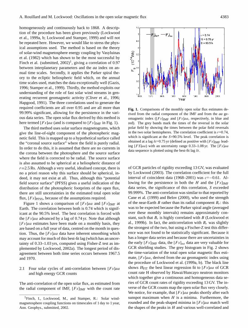
homogeneously and continuously back to 1868. A descrip-tion of the procedure has been given previously (Lockwoodet al., 1999a, b; Lockwood and Stamper, 1999) and will notbe repeated here. However, we would like to stress the phys-ical assumptions used. The method is based on the theoryof solar-wind magnetosphere energy coupling by Vasyluinaset al. (1982) which has shown to be the most successful byFinch et al. (submitted, 2002)1, giving a correlation of 0.97between interplanetary parameters and theaa index on an-nual time scales. Secondly, it applies the Parker spiral the-ory to the ecliptic heliospheric field which, on the annualtime scales used, matches the data exceptionally well (Gazis,1996; Stamper et al., 1999). Thirdly, the method exploits ourunderstanding of the role of fast solar wind streams in gen-erating recurrent geomagnetic activity (Cliver et al., 1996;Hapgood, 1991). The three correlations used to generate therequired coefficients are all over 0.95 and are all more than99.99% significant, allowing for the persistence in the vari-ous data series. The open solar flux derived by this method ishere termed[Fs]aa (and is compared to[Fs]IMF in Fig. 1).

The third method uses solar surface magnetograms, whichgive the line-of-sight component of the photospheric mag-netic field. This is mapped up to a hypothetical surface calledthe “coronal source surface” where the field is purely radial.In order to do this, it is assumed that there are no currents inthe corona between the photosphere and the source surfacewhere the field is corrected to be radial. The source surfaceis also assumed to be spherical at a heliospheric distance ofr=2.5 Rs. Although a very useful, idealised concept, there isno a priori reason why this surface should be spherical, in-deed, it may not exist at all. Thus, although this “potentialfield source surface” (PFSS) gives a useful indication of thedistribution of the photospheric footprints of the open flux,there are still uncertainties in the estimated total open solarflux, [Fs]PFSS, because of the assumptions required.

Figure 1 shows a comparison of[Fs]aa and [Fs]IMF atEarth. The correlation between both is 0.74 which is signif-icant at the 90.5% level. The best correlation is forced withthe [Fs]aa advanced by a lag of 0.74 yr. Note that although[Fs]aa estimates have been made on a monthly basis, theyare based on a full year of data, centred on the month in ques-tion. Thus, the[Fs]aa data have inherent smoothing whichmay account for much of this best-fit lag (which has an uncer-tainty of 0.33–1.03 yrs, computed using Fisher-Z test as im-plemented by Lockwood, 2002a). The longest period of dis-agreement between both time series occurs between 1967.5and 1970.

2.1 Four solar cycles of anti-correlation between[Fs]aa

and high energy GCR counts

The anti-correlation of the open solar flux, as estimated fromthe radial component of IMF,[Fs]IMF with the count rate

1Finch, I., Lockwood, M., and Stamper, R.: Solar wind-magnetosphere coupling functions on timescales of 1 day to 1 year,Ann. Geophys., submitted, 2002.

Figure 1. Comparisons of the monthly open solar flux estimates derived from the radial component of the IMF and from the aa geomagnetic index ([Fs]IMF and [Fs]aa, respectively, in blue and red). The grey bands mark the times of the reversal in the solar polar field by showing the times between the polar field reversals in the two solar hemispheres. The correlation coefficient is r = 0.74, which is significant at the S = 90.5% level. The peak correlation is obtained at a lag δt = 0.75 yr (defined as positive with [FS]IMF leading [FS]aa) with an uncertainty range 0.33-1.08yr. The [Fs]aa data sequence is plotted using the best-fit lag δt.

Fig. 1. Comparisons of the monthly open solar flux estimates de-rived from the radial component of the IMF and from theaa ge-omagnetic index ([Fs]IMF and [Fs]aa, respectively, in blue andred). The grey bands mark the times of the reversal in the solarpolar field by showing the times between the polar field reversalsin the two solar hemispheres. The correlation coefficient isr=0.74,which is significant at theS=90.5% level. The peak correlation isobtained at a lagδt=0.75 yr (defined as positive with[Fs]IMF lead-ing [FS]aa) with an uncertainty range 0.33–1.08 yr. The[Fs]aa

data sequence is plotted using the best-fit lagδt .

of GCR particles of rigidity exceeding 13 GV, was evaluatedby Lockwood (2003). The correlation coefficient for the fullinterval of coincident data (1968–2001) wasc=−0.61. Al-lowing for the persistence in both theH and the[Fs]IMFdata series, the significance of this correlation,S exceeded99.999%. The anti-correlation was similar to that reported byCane et al. (1999) and Belov (2000), who used the strengthof the near-EarthB rather than its radial componentBr : thiswas to be expected because the Parker spiral angle (averagedover these monthly intervals) remains approximately con-stant, such thatBr is highly correlated withB (Lockwood etal., 1999b). In fact, the anticorrelation withBr was slightlythe strongest of the two, but using a Fischer-Z test this differ-ence was not found to be statistically significant. Because ithas a longer data series and because there are uncertainties inthe early[Fs]IMF data, the[Fs]aa data are very valuable forGCR shielding studies. The grey histogram in Fig. 2 showsthe time-variation of the total open solar magnetic flux esti-mate,[Fs]aa, derived from theaa geomagnetic index usingthe procedure of Lockwood et al. (1999a, b). The black lineshowsHFIT the best linear regression fit to[Fs]aa of GCRcount rate H observed by Hawai/Huncayo neutron monitorswhich together give a continuous and homogeneous data se-ries of GCR count rates of rigidity exceeding 13 GV. The in-verse of the GCR counts map the open solar flux very closely.We notice, for example, that[Fs]aa peaks shortly after eachsunspot maximum whenH is a minima. Furthermore, therounded and the peak-shaped minima in[Fs]aa match wellthe shapes of the peaks inH and various well-correlated and


Figure 2. Variations of monthly means of solar, heliospheric and cosmic ray data since 1950. The grey histogram gives the open solar magnetic flux [Fs]aa, deduced from the aa geomagnetic index using the method of Lockwood et al. (1999a; b). The black line is HFIT the best fit of the anti-correlated cosmic ray counts H, observed by the equatorial Huancayo and Hawaii neutron monitors (which form a homogeneous data sequence on positively-charged GCRs with rigidities exceeding 13GV). The black histogram gives the sunspot number, R for comparison.

20 21 22

19

18 23

Fig. 2. Variations of monthly means of solar, heliospheric and cos-mic ray data since 1950. The grey histogram gives the open solarmagnetic flux[Fs]aa, deduced from theaa geomagnetic index us-ing the method of Lockwood et al. (1999a, b). The black line isHFIT, the best fit of the anti-correlated cosmic ray countsH , ob-served by the equatorial Huancayo and Hawaii neutron monitors(which form a homogeneous data sequence on positively-chargedGCRs with rigidities exceeding 13 GV). The black histogram givesthe sunspot numberR for comparison.

short-lived peaks, and minima appear in both[Fs]aa andHFIT. Monthly averages of[Fs]aa andH give a correlationcoefficientr of =−0.777 which means that 60% of the vari-ation in the cosmic ray variation is explained (in a statisticalsense) by the open solar flux. Allowing for the persistencein both theH and the[Fs]aa data series, the significance ofthis correlation,S exceeds 99.999% (i.e. there is less than a0.001% probability that this result was obtained by chance).

2.2 Disagreements between the estimates of the open fluxand cosmic ray counts at Earth in solar cycle 20

As we can see in Fig. 2 the main differences between thevariations of[Fs]aa and the best fit cosmic ray fluxes,HFIToccur on the descending phase of solar cycle 19 and through-out the anomalous solar cycle 20. It is interesting to note thatinitial studies did not find a good correlation between GCRsand the IMF (Hedgecock, 1975) but more recent data showthe IMF to be a more dominant factor than, for example, thetilt of the heliospheric current sheet (which is itself well cor-related withFs) (Cane et al., 1999; Belov, 2000). Here wereport similar but less significant disagreements betweenH

and[Fs]aa in the same period of time. Figure 1 shows that[Fs]aa goes though a maximum in the ascending phase ofsolar cycle 20 that is not reflected in[Fs]IMF (cf. Fig. 1) butis seen in a corresponding minimum in the cosmic ray counts(cf. Fig. 2). Additionally, in the descending phase of cycle 20(1971–1975),[Fs]IMF goes through a maximum neither re-flected with the same proportion in[Fs]aa norH .

2.3 The 22-year periodicity

The observed GCR fluxes show a marked 22-year cycle, withalternate peaked and rounded maxima (which, becauseH

is anti-correlated with[Fs]aa appear as V- and U-shapedminima of HFIT in Fig. 2). This has been attributed to theeffect of the drift term in the transport equation which hasbeen postulated to dominate the GCR shielding for 6–7 yearsaround solar mininum (the quiet heliosphere), the differencesbetween odd and even numbered cycles arising from the factthat the heliospheric field polarity A reverses shortly aftereach sunspot maximum: U- and V-shaped GCR maximaare expected forqA>0 andqA<0, respectively (Jokipii etal., 1977; McDonald et al., 1993). At solar maximum theparadigm of the quiet heliosphere (dominated by the effectsof the guiding centre, gradient and curvature drift motionsand quasi-steady corotating interaction regions CIRs) doesnot apply. In this diffusive mode of sunspot maximum, tran-sient events are thought to dominate and while drifts arethought to have still high magnitudes they are less globallycoherent.

Figures 1 and 2 show that alternate U- and V-shaped min-ima are also seen in both[Fs]aa and[Fs]IMF , implying thata 22-yr cycle was also a feature of the open solar magneticflux emergence. It appears therefore that on top of a twenty-two-year pattern in the polarity of the Sun’s magnetic field,a twenty-two-year pattern is also seen in the time varyingquantity of open field lines threading a sphere centred on theSun and passing at 1 AU. This correspondence could follownaturally from an eleven-year variation in the cosmic ray fluxresulting from a series of outward propagating transients, oreven merged transients as first identified by McDonald etal. (1981) but not from a drift-induced 11-year modulationas proposed by Jokipii et al. (1977). The presence of chargesign dependent effects around the years of solar minimum,1995.5–1998, has been recently demonstrated convincinglyby Heber et al. (1999), using Ulysses Kiel Electron Tele-scope data. Galactic comic electrons also show this 22-yrcycle and, having the opposite chargeq, the drift theory pre-dicts that this should be in antiphase with the nucleon GCRvariation (Evenson, 1998). Measurements of 2.5 GV protonsand electrons during the first fast latitudinal scan (1994.7–1995.6) revealed a small but clear latitudinal gradient in thetime series not observed in the electron data (Heber et al.,1999) and in agreement with a drift-mode according to Fer-reira et al. (2003) (where protons are expected to drift in fromthe poles during these years ofA>0). In the same paperHeber et al. showed that between 1995.5 and 1998 the elec-tron time series presented greater sensitivity to variations inthe tilt of the HCS than the proton time series in agreementwith negative particles propagating inward along the cur-rent sheet (Heber et al., 1999). These results have revealedcharge-sign dependent effects in the years with an extrapo-lated HCS tilt smaller than 20 degrees and do not allow anyconclusions to be drawn on their direct relevance to the 11-year modulation effect. The more recent Ulysses KET datarecorded during the global solar polarity change was also


analysed and shows a charge-sign dependence before and af-ter the years of solar maximum (Heber et al., 2003). Heberet al. (2003) noticed that the relative variation of the electronand proton counts along the Ulysses orbit phased in for twoand a half years at solar maximum but phased out outsidethis period in the transition years from solar maximum tosolar minimum mode. The most promising direct detectionof a charge-sign dependent effect at solar maximum was ob-tained by Clem and Evenson (2002), using the positron abun-dance recently measured by the LEE/AESOP payload (LowEnergy Electrons/Anti-Electron Sub Orbital Payload) aboarda balloon flight. As seen in Fig. 5 of their paper a clear tran-sition in the abundance of positron at Earth is seen duringpolarity reversal. The result is based, however, on one set ofmeasurements in the newA<0 polarity state, and new mea-surements are needed to obtain the average abundance of thecurrent polarity state. These new results obtained in the yearsbefore, during and just after solar maximum suggest a pos-sible important role of charge-sign dependent effects in theyears of transition from GCR minimal to maximal values.As mentioned earlier Wibberenz et al. (2002) have combinedthese drift-associated effects and the time-dependent tran-sient modulators by postulating that the background driftsset the global distribution of cosmic rays in the heliospherewhich is then modulated by the outwardly propagating tran-sients. We are lacking, however, observations that would al-low for a proper determination of the relative role of driftsand propagating diffusive barriers in generating the 11-yearcosmic ray cycle. The close correspondence between the var-ious open flux estimates and the cosmic ray flux at Earth inthe last two solar cycles is striking and could reveal funda-mental properties of the photospheric origin and low coronagenerating/redistribution mechanisms of both the solar openmagnetic field lines and their associated GCR modulators.We also think that a comparison of the anomalous cosmic raycycle, a period when the open flux does not follow the GCRflux as well (solar cycle 20), with the two recent solar cycles,could reveal interesting features on the origin of the 11-yearcosmic ray cycle and perhaps put this 11-year open flux-GCRcorrespondence in context with recent results on charge-signdependence. These claims will be addressed thoroughly in aforthcoming article.

Here we investigate the two possibilities that the 22-yr cy-cle in GCRs may result from the polarity dependent drifts orthat it is related to open flux emergence from the Sun.

Section 3 discusses corresponding periodicities detected inthe large-scale magnetic field and their relation to the solarsurface dynamics with periodicities observed in cosmic rayscounts. Section 4 presents more correlative work betweenthe finer time series structure of the open flux and cosmicray counts measured at Earth. Section 5 presents quantitativework on the lags observed between the fluctuations of thesolar magnetic field and cosmic ray measurements at 1 AU.

3 Periodicities in the large-scale magnetic field and incosmic ray counts at Earth

3.1 1–2-year quasi-periodicities

The Sun’s large-scale magnetic field and its proxies areknown to undergo substantial variations on time scales muchless than a solar cycle but longer than the 27-day rotationperiod. For instance, Gnevyshev argues that each solar cycleexhibits two peaks of maximum activity separated by 2–3 yr,a feature present in large sunspots, major flares, coronalgreen-line emission and geomagnetic activity (Gnevyshev,1967, 1977). Storini et al. (1997) detected double-peakedstructures in the cosmic ray flux during solar cycles 19–22,with intervening “gaps” coinciding with the time of helio-magnetic polarity reversal. Although the effects describedby Gnevyshev and subsequent authors are related to varia-tions in the Sun’s large-scale magnetic field occuring at andjust after sunspot maximum, flucutations on time-scales of1–3 yr are also present at other phases of the solar cycle ap-pearing from time to time and have been detected in vari-ous solar wind parameters (Richardson, 1994), as well asauroral records (Silvermann and Shapiro, 1983). Recently,Lockwood (2001) has suggested that the field variations of∼1 year in duration associated with medium-term eventsmay be related to the oscillations close to the base of the solarconvection zone observed by the SOHO spacecraft (Howe etal., 2000). In fact, a recent study suggests that periodicitiesof 1.3–1.4 yr may occasionally appear from 1-yr decayingstochastic processes associated with the emergence of activeregions on the solar surface (Wang and Sheeley, 2003).

3.2 The imprint of the open solar flux in GCR fluxes

A strong oscillation in GCR fluxes of periodT =1.68 yr (fre-quency, f =0.595 yr−1=9 nHz) has been reported recentlyand related to similar oscillations in solar surface features(Valdes-Galicia et al., 1996; Valdes-Galicia and Mendoza,1998). This periodicity has also been found in the coronalhole area (McIntosh et al., 1992; Maravilla et al., 2001). Herewe remove the dominant solar cycle periodicity using a high-pass filter (f >0.2 yr−1, T <5 yr) and use non-parametric andparametric spectral estimations to investigate this oscillation.In addition to application to the GCR data series, these meth-ods were applied to the open solar flux derived from bothsolar surface magnetograms by the PFSS (Potential FieldSource Surface) method (Wang and Sheeley, 1995) and thenear-Earth IMF observations (Lockwood, 2003).

Results of a non-parametric spectral estimation of the fil-tered time series, made using Fourier analysis, are shown inFig. 3. For this 22-year period (1972–1994) the 1.68-year os-cillation is the strongest feature in the power spectra of bothGCR fluxes and of the open flux, once the dominant 11-yearsolar cycle is suppressed by the filter. For this 22-yr inter-val, power spectra have a frequency resolution of 0.048 yr−1.The spectra are offset vertically for clarity. From bottomto top they are for: the Climax neutron monitor (>3 GV)


Figure 3. Stacked power spectra for 1972-1994. All data have been Fourier analysed after being passed through a high pass filter (f > 0.2 yr-1) to suppress the solar cycle variation. From bottom to top: Climax neutron monitor (>3GV) counts, C (blue); Moscow neutron monitor (>4GV) counts, M (red); Huancayo/Hawaii neutron monitor (>13GV) counts, H (black and yellow dashed); open solar flux deduced from photospheric magnetograms by the PFSS method, [Fs]PFSS (green); open solar flux deduced from the radial interplanetary magnetic field measured near Earth, [Fs]IMF (black); the aa geomagnetic index (light blue and mauve). Vertical dashed lines mark periods of 1.68 yr, 1.30 yr, 1.00 yr and 0.50 yr.

Fig. 3. Stacked power spectra for 1972–1994. All data havebeen Fourier analysed after being passed through a high pass filter(f >0.2 yr−1) to suppress the solar cycle variation. From bottom totop: Climax neutron monitor (>3 GV) counts,C (blue); Moscowneutron monitor (>4 GV) counts,M (red); Huancayo/Hawaii neu-tron monitor (>13 GV) counts,H (black and yellow dashed); opensolar flux deduced from photospheric magnetograms by the PFSSmethod,[Fs]chemPFSS (green); open solar flux deduced from theradial interplanetary magnetic field measured near Earth,[Fs]IMF(black); theaa geomagnetic index (light blue and mauve). Verticaldashed lines mark periods of 1.68 yr, 1.30 yr, 1.00 yr and 0.50 yr.

counts, C (blue); the Moscow neutron monitor (>4 GV)counts, M (red); the Huancayo/Hawaii neutron monitors(>13 GV) counts,H (black and yellow dashed); the opensolar flux deduced from photospheric magnetograms by thePFSS method,[Fs]PFSS(green); the open solar flux deducedfrom the radial interplanetary magnetic field measured nearEarth,[Fs]IMF (black); and theaa geomagnetic index (lightblue and mauve). The vertical dashed lines mark the fre-quencies corresponding to periodT of 1.68, 1.3, 1.0 and0.5 years. All spectra show a peak atT =1.68 yr, except for[Fs]PFSS which shows enhanced power at this period butpeaks for the adjacent quantised period of 1.54 yr. Somespectra also show a peak atT =1.3 yr which is seen in so-lar wind speed and geomagnetic activity (Richardson et al.,1994; Mursula and Zieger, 2000; Lockwood, 2001). Theaageomagnetic activity index also shows a strong peak at 0.5 yr,arising from the effect of the Earth’s axial tilt on coupling be-tween the solar wind and the Earth’s magnetosphere (Russelland McPherron, 1973). Given the strong equinoctial effectthat this mechanism causes in geomagnetic activity, it is in-teresting to note that the power in the variation atT =0.5 yris only 50% bigger than that inaa at T =1.68 yr. Theaa in-dex also shows a weak peak at 1.0 yr which is most likelya result from ionospheric conductivity variations at the twomagnetometer sites used to compile the index. Weak annualvariations are also seen in the cosmic ray data from all the

sites employed: these indicate that either the corrections toallow for the effect of atmospheric pressure on raw neutroncounts have not completely suppressed the seasonal variationintroduced by this effect, or there is a strong yearly effect ofthe inclination of the Earth (Nagashima et al., 1985).

The parametric spectral estimation was also made us-ing the maximum entropy method (MEM). The time se-ries is modelled parametrically and then processed with thecondition that the entropy of the original random time seriesis maximised (Kay and Marple, 1981). This has the effect of“flattening” the power spectrum and can provide a frequencyspectrum with sharp spectral features. MEM can be unreli-able if the order of the parametric model used is too small ortoo big: too small a model order will give a spectrum withbad resolution, too big a model order can lead to a spectrumwith “artificial peaks” (with some spectral line splitting oc-curring). Some criteria of model order selection were usedto give an idea as to what model order should be selected fora particular time series. The MEM procedure was applied tothe filtered Climax neutron monitor counts,C, the open solarflux data deduced from surface magnetograms by the PFSSmethod,[Fs]PFSS, and to the open solar flux deduced fromthe radial interplanetary field measured at Earth,[Fs]IMF .As for the Fourier analysis, in all MEM spectra the variationatT =1.68 yr in the corresponding time series is the most im-portant peak once the 11-year solar cycle variation is filteredout. This oscillation therefore appears to be a characteristicimprint of the open solar flux on the GCRs. Application of aband-pass filter (5<T <1 yr) onH andC, which would effec-tively remove the overall 11-yr solar cycle variation, wouldleave a time series1H and1C dominated by the 1.68-yroscillation in an almost synchronised way to1[Fs]IMF withprobable exact phase variations. We investigate this questionin Sect. 4 by means of correlation analysis.

Figure 4 shows the variation of the power spectral densi-ties of the cosmic ray count rates, two open solar flux esti-mates (1[Fs]aa is not used because of the smoothing inher-ent in its derivation – see Lockwood et al., 1999a, b) and thetilt of the heliospheric current sheet. These are obtained fromthe Fourier analysis (using 11-year sliding data intervals) andplotted here in spectrogram format. The time of a particularpower density is taken as the middle date of each 11-yearwindow. An 11-year window was taken as a compromise be-tween time and frequency resolution (windowing effects arediscussed below), where the length of the window taken ofcourse determines the starting and ending date of the variousspectrograms. The peak around frequencyf =1/1.68 yr−1 isa persistent and strong feature (>10%2 Hz−1) in all spec-trograms except for the tilt of the heliospheric current sheetwhich has for this frequency a power spectral density lessthan 6%2 Hz−1 and appearing much later in the solar cycle.We also notice that during the period wheref =1/1.68 yr−1

appears strongest in all data sequences, the heliospheric cur-rent sheet reveals a frequency of∼1./0.72 yrs not seen in thecosmic ray spectrograms corroborating the results of Caneet al. (1999), who found that the overall correlation be-tween HCS tilt and cosmic ray count rates was low. The


H(>13GV) C(>3GV)

a b

c d

e

Fig. 4. Spectrograms showing contours of power spectral density as a function of date and frequency,f . The dashed white lines in eachpanel show periods of 0.5, 1.0, 1.33 and 1.68 years. Power spectra are computed for 11-yr periods, centred on the dates shown on thehorizontal axes. Plots are for:(a) Climax neutron monitor (>3 GV) counts,C; (b) Huancayo/Hawaii neutron monitor (>13 GV) counts,H ;(c) open solar flux deduced from the radial interplanetary magnetic field measured near Earth,[Fs]IMF ; (d) open solar flux deduced fromphotospheric magnetograms by the PFSS method,[Fs]PFSS; and(e) the heliospheric current sheet tilt angle.

correspondence between the spectrograms for the cosmic raycounts and the1[Fs]IMF spectrogram is remarkable: mostfrequencies seen in Fig. 4c also appear in Figs. 4a and b.The spectrograms are also quite similar to that obtained byKudela et al. (2002) using wavelet transforms as their spec-tral method. However, the periodicity pattern highlighted byMursula and Zieger (1999) is not reproduced clearly here.Figure 5 shows the time variations of spectral power at period

1.68 yr. Results are shown for GCR countsC, M and H

(respectively,>3 GV, >4 GV, >13 GV), the open solar fluxestimates[Fs]IMF and [Fs]PFSSand the HCS tilt. Similarvariations are seen in all parameters with peaks at the timeof peak sunspot number (shown by the coloured histogramat the bottom of the plot); however, the peak in 1968 is pro-portionally weaker. The top panel uses 11-year sliding win-dows (the same as the spectrograms shown in Fig. 4), which


Figure 5. Time variations of the power spectral density around the period of 1.68 years (1.55yr ≤ T ≤ 1.81yr) from analysis of (top) 11-year segments of data and (b) 6-year segments of data. The variations are shown using the same line colour-coding scheme as figure 3. The sunspot number variation is shown for comparison. Power spectral densities have been scaled to that for the Climax counts, C, using the best least-squares linear regression fits of the time variations.

a)

b)

Fig. 5. (a) Time variations of the power spectral density aroundthe period of 1.68 years (1.55 yr≤T ≤1.81 yr) from analysis of (top)11-year segments of data and(b) 6-year segments of data. Thevariations are shown using the same line colour-coding scheme asFig. 3. The sunspot number variation is shown for comparison.Power spectral densities have been scaled to that for the Climaxcounts,C, using the best least-squares linear regression fits of thetime variations.

maintains high frequency resolution but is comparable to thesolar cycle. In the lower panel we repeat using 6-year win-dows (the same as used in Figs. 7, 8, 9 and 10 described later)with lower frequency but higher time resolution. The timevariations are, generally speaking, similar at sunspot maxi-mum; although for the first cycle the smaller peak is in thedeclining phase.

4 Procedure of the correlation analysis

The presence of corresponding quasi-annual periodicities inboth cosmic ray and open solar flux data motivated a moredetailed correlative study. We present in this section the re-sults of a window-by-window correlation analysis betweenthe open solar flux estimates and the cosmic ray counts mea-sured by the Climax and Huancayo/Hawaii neutron monitors

C andH , respectively. Open flux estimates derived from ge-omagnetic activity and radial IMF observations,[Fs]aa and[Fs]IMF are both used. The correlation analysis of[Fs]aa

with H andC is limited to their unfiltered data due to the timeresolution of[Fs]aa>1 yr but these data provide a longeroverall interval. However, the correlation analysis of[Fs]IMFwith H andC can be carried out on both the detrended data(after application of a band pass filter 5<T <1 yr) and on theraw data.

4.1 Description of the window by window cross-correlation analysis

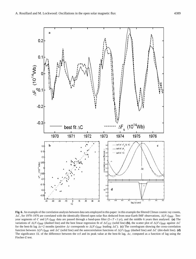
To evaluate the time-variation of the cross-correlation coeffi-cient between open solar flux estimates and the neutron mon-itor count rates at Earth over the last four completed solarcycles, we employ the cross-correlation analysis illustratedby Fig. 6. This example shows a cross-correlation between1[Fs]IMF and1C, where the notation1X refers to param-eter X after passing through a high band-pass filter. Thefilter used has a pass-band of 4 yrs. FHWM is centred on3 yrs. Here we filter 11-year segments of the data of whichwe then employ the middle 6 years, thereby avoiding end ef-fects of the sliding window. Figure 6a shows an example ofa temporal variation of1[Fs]IMF (dashed line) and the bestlinear regression fit1Cf it (solid line) and Fig. 6b shows thesame data in scatter plot format for the best-fit lag1t (posi-tive 1t corresponds to1[Fs]IMF leading1C) which equals2 months in this case; the line in Fig. 6b shows the best-fitregression used to scale the best fit,1Cf it , from 1C. Fig-ure 6c shows the correlogram giving the cross-correlationfunction (ccf) between1[Fs]IMF and1C (solid line) andthe autocorrelation functions (acf) of1[Fs]IMF (dashed line)and1C (dot-dash line), all shown as a function of lag. Fig-ure 6d shows the significanceSL of the difference betweenthe ccf and its peak value at the best-fit lag,1t , computed asa function of lag using the Fischer-Z test. The uncertainty,δ,is set by the points whereSL rises above 90% and the ccf be-comes significantly lower than its peak value. Further detailsof this correlation procedure are given by Lockwood (2002a).In this case the correlation coefficientc=0.93 which, allow-ing for persistence, is significant at theS>99.6% level.

4.2 Window by window cross-correlation analysis ofC andH with [Fs]aa

Figures 7 and 8 show the results of applying this procedure to[Fs]aa and GCR counts of rigidity exceeding, respectively,13 GV (H , from the Huncayo/Hawai neutron monitor) and3 GV (C, from the Climax neutron monitor). The top panelof both figures shows the raw data series, whereas the sec-ond panel shows the same data after application of the band-pass filter. Considerable variability can be seen in the GCRcounts in the 1–5 yr pass band in the1C and 1H series.However, the inherent one year smoothing of[Fs]aa is re-vealed by the relative lack of variation in1[Fs]aa (red linein Figs. 7b and 8b) when the main solar cycle variation is


a).

b).

c).

d).

a

b c

d

∆t

Fig. 6. An example of the correlation analysis between data sets employed in this paper: in this example the filtered Climax cosmic ray counts,1C, for 1970–1976 are correlated with the identically filtered open solar flux deduced from near-Earth IMF observations,1[Fs]IMF . Ten-year segments ofC and [Fs]IMF data are passed through a band-pass filter (5<T <1 yr), and the middle 6 years then analysed.(a) Thevariations of1[Fs]IMF (dashed line) and the best linear regression fit of1CFIT (solid line) (b), the scatter plot of1[Fs]IMF against1C

for the best-fit lag1t=2 months (positive1t corresponds to1[Fs]IMF leading1C). (c) The correlogram showing the cross-correlationfunction between1[Fs]IMF and1C (solid line) and the autocorrelation functions of1[Fs]IMF (dashed line) and1C (dot-dash line).(d)The significanceSL of the difference between the ccf and its peak value at the best-fit lag,1t , computed as a function of lag using theFischer-Z test.


Figure 7. Results of the correlation analysis of Huancayo/Hawaii neutron monitor (>13GV) counts H and the open solar flux deduced from the geomagnetic aa index [Fs]aa. The grey bands mark the times of the reversal in the solar polar field by showing the times between the polar field reversals in the two solar hemispheres. From top to bottom, the panels show: (a). the variations of [Fs]aa (red) and HFIT, the best linear regression fit of H to [Fs]aa (blue); (b). the band-pass filtered variations ∆[Fs]aa (red) and ∆HFIT, the best linear regression fit of ∆H to ∆[Fs]aa (blue); (c) the lag of the peak correlation, δt; (d) the magnitude of the peak correlation coefficient |r|, and (e) the significance of that correlation, S. The mauve and the grey data points to the right of (c), (d) and (e) give the values for the full, raw data sequences shown in the top panel (in mauve) and the filtered data sequences (in grey). The correlation of ∆[Fs]aa and ∆H is low (r = 0.22) because of the smoothing inherent [Fs]aa, so only data points for [Fs]aa and H are shown in (c), (d) and (e), computed for each 6-year interval as shown in figure 5: data points in green have S ≥ 90% (the dotted line shown in the bottom panel), those in cyan have S < 90%.

a

b

c

d

e

Fig. 7. Results of the correlation analysis of Huancayo/Hawaii neu-tron monitor (>13 GV) countsH and the open solar flux deducedfrom the geomagneticaa index [Fs]aa. The grey bands mark thetimes of the reversal in the solar polar field by showing the times be-tween the polar field reversals in the two solar hemispheres. Fromtop to bottom, the panels show:(a) the variations of[Fs]aa (red)andHFIT, the best linear regression fit ofH to [Fs]aa (blue); (b)the band-pass filtered variations1[Fs]aa (red) and1HFIT, the bestlinear regression fit of1H to 1[Fs]aa (blue); (c) the lag of thepeak correlation,δt ; (d) the magnitude of the peak correlation coef-ficient |r|, and(e) the significance of that correlation,S. The mauveand the grey data points to the right of (c), (d) and (e) give thevalues for the full, raw data sequences shown in the top panel (inmauve) and the filtered data sequences (in grey). The correlationof 1[Fs]aa and1H is low (r=0.22) because of the smoothing in-herent[Fs]aa, so only data points for[Fs]aa andH are shownin (c), (d) and (e), computed for each 6-year interval as shown inFig. 5: data points in green haveS≥90% (the dotted line shown inthe bottom panel), those in cyan haveS<90%.

removed after application of the band-pass filter: the shortestperiod of oscillation is at least 3 years as explained above.In fact, the overall cross-correlation coefficient is very low:|r|=0.22 for 1[Fs]aa with 1HFIT and |r|=0.18 1[Fs]aa

with 1CFIT. We present in Figs. 7d and 8d the time varia-tions of the cross-correlation coefficients|r| for [Fs]aa withH and C (all unfiltered), respectively. These cross-correlationcoefficients have high values (|r|>0.6) with a high signifi-cance (S>80%) throughout most of the interval where cos-mic ray measurements are available. A continuous and sig-nificant decrease is seen, however, in both|r| sets between1968 and 1977, confirming the disagreements already visible

Figure 8. The same as figure 7, for the correlation analysis of Climax neutron monitor (>3GV) counts C and the open solar flux deduced from the geomagnetic aa index [Fs]aa.

a

b

c

d

e

Fig. 8. The same as Fig. 7, for the correlation analysis of Climaxneutron monitor (>3 GV) countsC and the open solar flux deducedfrom the geomagneticaa index[Fs]aa.

in the raw time series (Fig. 2). The same window-by-windowcross-correlation analysis of unfiltered data was carried outwith [Fs]IMF instead of[Fs]aa and gives very similar results(blue and green lines of Figs. 9 and 10). The differences seenin solar cycle 20 between the variation of the total amount ofopen field lines in the heliosphere and the GCR count ratesat Earth are statistically the same for the two estimates of thetotal open flux. The middle panels (c) of Figs. 7, 8, 9 and 10give the lags of peak correlation with uncertainties as derivedin Fig. 6. On the right hand-side of panels (c), (d) and (e) ofthe figures is given respectively, the best fit1t , the correla-tion coefficient|r|, and the significanceS for the full datasequences: the mauve and grey points are for the unfilteredand the filtered data shown in panels (a) and (b), respectively.

4.3 Window by window cross-correlation analysis ofC andH with [Fs]IMF , as well as the filtered time series1C

and1H with 1[Fs]IMF

To investigate the imprint of the different oscillations in theopen solar flux to the GCR counts further, the window-by-window cross-correlation procedure was applied to the de-trended open solar flux1[Fs]IMF with the detrended cosmicray counts1H and 1C. (As mentioned above the inher-ent smoothing in[Fs]aa does not allow us to use it for thisanalysis). 11-year intervals of data were passed through thesame band-pass filter (5<T <1 yr) and, to avoid edge effects,


Figure 9: The same as figure 7, for the correlation analysis of Huancayo/Hawaii neutron monitor (>13GV) counts H and the open solar flux deduced from the radial component of the IMF [Fs]IMF. The correlation of ∆[Fs]IMF and ∆H is high (r = 0.61) so analysis of ∆[Fs]IMF and ∆H are shown in (c), (d) and (e) (in addition to that for the unfiltered data, [Fs]IMF and H, again shown in green and cyan): those in black have S ≥ 90% (the dotted line shown in the bottom panel), those in red have S < 90%.

b

a

c

d

e

Fig. 9. The same as Fig. 7, for the correlation analysis of Huan-cayo/Hawaii neutron monitor (>13 GV) countsH and the open so-lar flux deduced from the radial component of the IMF[Fs]IMF .The correlation of1[Fs]IMF and1H is high (r=0.61) so analysisof 1[Fs]IMF and1H are shown in (c), (d) and (e) (in addition tothat for the unfiltered data,[Fs]IMF andH , again shown in greenand cyan): those in black haveS≥90% (the dotted line shown in thebottom panel), those in red haveS<90%.

the middle 6 years were then cross-correlated. The resultsof these cross-correlations are shown in Figs. 9 and 10. Thegreen/light blue lines in parts (c), (d) and (e) are for unfil-tered dataC and[Fs]IMF , the black/red lines are for the fil-tered data1[Fs]IMF (red) and1CFIT: the green and blacksegments are for correlations of significanceS exceeding the90% threshold (the horizontal dotted line in part e), the redand light blue segments are forS≤90%.

The correlation for the filtered data is strong and signifi-cant (S>90%, shown in black) at all solar maxima (when thepower at 1.68 yrs is greatest, see Fig. 8), as well as the min-ima for solar field polarityA>0 (around 1975 and 1990), butfalls to S<90% (shown in red) for the minimum withA<0(around 1987). Figure 5 shows that this lack of correlationis not caused by a lack of power in the 1.68 yr oscillation, itbeing comparable to during the other two minima. It appearsthat for periods dominated by transient events at solar maxi-mum and for periods dominated by the GCR drifts expectedat solar minimum forqA>0 (inflows from the heliosphericpoles to Earth), the 1.68-yr oscillation in the open solar fluxleaves a clear and dominant imprint on the GCR fluxes. How-ever, for the minimum withqA<0, when drifts associated

Figure 10: The same as figure 9, for the correlation analysis of Climax neutron monitor (>3GV) counts C and the open solar flux deduced from the radial component of the IMF [Fs]IMF.

b

a

c

d

e

Fig. 10. The same as Fig. 9, for the correlation analysis of Climaxneutron monitor (>3 GV) countsC and the open solar flux deducedfrom the radial component of the IMF[Fs]IMF .

with the smooth background field are predicted to force cos-mic rays to propagate along the equatorial heliospheric cur-rent sheet to Earth the imprint of the 1.68-year oscillationin open flux is considerably weaker and/or more confused.Thus, in the imprint of the 1.68-year variation we seem tofind evidence forqA-dependent drifts. However, the oscilla-tions detected spectrally in the tilt of the heliospheric currentsheet (1982–1995) do not appear in the cosmic ray counts atEarth in this particular period of predicted HCS propagation.An interesting issue is whether these frequencies should orshould not appear in the cosmic ray counts according to ourpresent understanding of the propagation of cosmic rays inthe heliosphere. The tilt angle has been used in many modelsof cosmic ray modulation as a time-dependent parameter inorder to solve Parker’s equation (e.g. Ferreira et al., 2003) orto provide a convenient way of relating the change in the dif-fusion coefficient to the evolving solar activity (Wibberenzet al., 2002). A spectral analysis of the cosmic ray counts’time series predicted by these various models in the period1980–1985 would perhaps clarify this point.

The correlation for the filtered data is strong before 1976.This could support suggestions that the earliest IMF datawere subject to a drift in their absolute calibration (Belov,2000) and that this lowers the correlation for unfiltered data(the light blue segments). However, the same low cross-correlation coefficients are obtained for the open solar flux


from aa (Figs. 7 and 8), and so it seems that the effect is realand the mechanism linking the total amount of open fieldlines in the heliosphere to the time-variation of cosmic raysmeasured at Earth for some reason acted differently in so-lar cycle 20 (than in solar cycles 19, 21, 22 and 23). Sucha hypothesis is valuable considering that solar cycle 20 ischaracterised by an overall lower activity and a longer mag-netic field reversal than in other cycles (Fig. 6). Wibberenzet al. (2002) argue that this apparantly “anomalous” responseof the cosmic rays in solar cycle 20 is due to the differenttimes for particles to enter into the depleted regions of theheliosphere by diffusion and drift mechanisms in the twodifferent magnetic polarities of the Sun. Periods of nega-tive polarity A<0 when inflows are thought to occur alongthe HCS (such as the descending phase of solar cycle 20)should be characterised by long recovery processes. Thepresence of numerous weak field increases, with time lengthsless than characteristic recovery times between them, wouldthen be more effective in preventing sunward cosmic rayspropagation. This interpretation should, in principle, lead tothe GCR depression seen even with the considerably weakerIMF strength of this solar cycle (Fig. 1).

5 The presence of varying lags between cosmic ray fluxat Earth and 1[Fs]IMF

The study of lag times between changes in the quantity ofopen field lines near the Sun (progressively dragged out inthe heliosphere by the solar wind) and the subsequent re-sponse of cosmic rays is crucial to any approach of GCRsolar modulation where diffusion mechanisms have a domi-nant role.

Figures 7, 8, 9 and 10 show interesting features concerningthe time-lag variation between the various cross-correlationsof the open solar flux estimates and cosmic ray counts atEarth. In studying these plots it should be remembered that[Fs]IMF leads[Fs]aa by 0.75±0.4 yr. A lag (1t>0) is ex-pected between open magnetic field and cosmic ray varia-tions because changes in the heliospheric field are carriedinto the heliosphere at the solar wind speed or less. Themode value of the distribution of the heliographic equatoris 370 km s−1, which corresponds to distances of the order of78 AU per year (Hapgood et al., 1991). This agrees well withthe typical speeds seen in the streamer belt by Ulysses: thespeeds seen by Ulysses in the polar regions are roughly twicethis at solar minimum, but at solar maximum the speeds be-come similar at all latitudes (Richardson et al., 1994). Studyof the time-lag for peak correlation between the open solarflux and cosmic ray counts at Earth can be used to inferroughly the locations of main modulation mechanisms as-sociated with the diffusion tensor in the adopted paradigmwhere changes in the open solar flux are propagated outwardat the solar wind speed. A simple look at the size of the errorbars in Figs. 7, 8, 9 and 10 shows that the following anal-ysis does not claim to be an exact study of lags; moreover,

as pointed out by Dorman et al. (1997, 2001), an accurateinterpretation of lags in terms of the size of the modulationregion should include the integral modulation effects of allmechanisms known to date. Figures 7c and 8c show the pre-viously discussed results of cross-correlating[Fs]aa with H

and C, as well as the detrended variations1[Fs]aa with1H and1C. The best-lag obtained for the overall cross-correlation is shown as pink and grey dots, respectively, onthe right-hand side of the sub-figure. A green/blue line rep-resents the time variation of the best-fit lag obtained for thewindow by window cross-correlation of[Fs]aa with H andC. The lag remains in all cases very high at about 8 monthswith considerable random fluctuations in the period of low-correlation coefficients. The time-lag has not changed sig-nificantly in the last 40 years and is similar to the overall lag.Noting that[Fs]aa leads[Fs]IMF by 0.75 yr, Figs. 7 and 8show no significant evidence for a non-zero lag.

Figures 9c and 10c show the results of cross-correlating[Fs]IMF with H and C (greeen/blue lines), as well asthe detrended variations1[Fs]IMF with 1H and1C (redand black lines). The overall lag obtained for[Fs]IMF(1t∼0) and 1[Fs]IMF is much smaller than for[Fs]aa.The green/blue lines in Figs. 9c and 10c show that the time-lags between[Fs]IMF andH or C do not remain constantthroughout the solar cycles but shift from values close to0.2 yr in (1971–1981) to very low values (1991–1996) intheqA>0 polarity states. The same general trend is noticedin the red/black lines corresponding to the cross-correlationof the detrended variations1[Fs]IMF with 1H and 1C,with additional big fluctuations appearing in theqA<0 po-larity state (1981–1991) for the cross-correlation with theHawai/Huncayo neutron monitors counts. These big varia-tions inqA<0 are features of the very poor cross-correlationobserved during this time period and therefore are artificial(leading to an unphysical point of value below zero, errorbars considered). It should be noted that if statistical er-rors are considered, all other best lag estimates have phys-ical values and the green/blue line values agree with theblack/red line values. Around 1980, a persistent value of1t=0.25±0.15 yr is observed, in this solar maximum pe-riod a solar wind speed of 370 km.s−1 would lead to a re-sponse of cosmic rays to diffusion mechanisms at around11–30 AU: this is consistent with where merged interactionregions have been seen to act as barriers to GCRs at this time(Burlaga, 1987; Heber et al., 2000). However, at the nextsolar maximum around 1991, both the1[Fs]IMF−1C and1[Fs]IMF−1H correlations show a shorter lag, which maybe an indicator that the response to changes in the open fluxby diffusion is somewhat closer in towards the Sun.

It should be noted that the strong IMF-GCR correlationspresented by Cane et al. (1999) and Belov (2000) were forzero lag.

The upper limit to1t for the filtered data places an esti-mate of the outer limit on the location of high energy GCRscattering processes. Figures 9c and 10c show that this upperlimit decreased from about 0.3 yr around 1980 to less than0.1 yr around 1995, the subsequent sunspot minimum with


A>0. This suggests that scattering processes of the inflow,thought to occur mainly over the poles forA>0, might havemoved inward from within 50 AU to within 10 AU. The rea-sons for this change are not understood. Both[Fs]aa and[Fs]IMF (Fig. 1) are of the order of 15% lower for the secondof these sunspot minima. This may allow the GCRs to reachcloser to the centre of the heliosphere before they are signif-icantly scattered. The study of these lags will be the subjectof following papers. For more information on lags we re-fer the readers to the extensive work of Dorman et al. (1997,1999, 2001), who have studied lags between features on theSun and GCRs by assuming the full integral nature of GCRmodulation.

6 Summary and conclusions

For all but the period 1968–1975, there is a strong and sig-nificant anti-correlation between the open solar flux, as de-rived from IMF observations or theaa geomagnetic index,and cosmic ray flux at Earth. This is true during most ofthe solar cycle phases of both magnetic field polarities andcould point to a more significant role of the open solar fluxin cosmic ray flux modulation than has been attributed todate. We notice an interesting fact, that is, the alternatepeaked and rounded maxima seen in the neutron GCR fluxtime series (giving a 22-year cycle), successfully attributedto the polarity-dependent drift component of the propagationmechanisms of cosmic rays in the heliosphere (see Heber,2000; Ferreira et al., 2003), is also seen in the variation ofthe two 1-AU open flux estimates presented here. This im-plies that the Sun has, as well as a twenty-two-year cycle inthe direction of its dipolar field, a twenty-two-year pattern inthe quantity of open field lines threading a sphere passing at1 AU. In the last four solar cycles at least, the Sun appears tohave reached low open flux values sooner after polarity re-versal inqA>0 polarity, leading to rounder minima than inqA<0 polarity.

In this paper, we have shown that the recently reported1.68-year variation in GCR fluxes is a persistent feature thatis linked to a similar variation in the open solar magnetic fluxestimated from the IMF strength at Earth or from the PFSSmethod using solar magnetograms. This imprint is strongestat solar maximum and cross-correlation analysis shows thatthere is a difference betweenqA>0 and qA<0 cycles atsunspot minimum. Thus, we find possible evidence for theeffects of polarity-dependent GCR drifts acting at least 3–4years around sunspot minimum. The close mapping betweenthe average IMF strength on such different time scales is sig-nificant: we confirm the possibility that the variation of thetotal flux in the heliosphere is a good proxy to the overallvariation of diffusion mechanisms affecting the propagationof 3–10 GV cosmic rays, at least in the inner heliosphere.The 1.68-yr variation has only a very weak power for 1982–1986 and is non-existent for the period 1989–1993, in thespectral analysis of the HCS tilt angle. In contrast, the pe-riod is present in the GCR data during these time intervals.

A spectral analysis of the cosmic ray counts’ time series pre-dicted by the various models which make use of the HCS tiltangle (Ferreira et al., 2003) in the period 1980–1986 wouldperhaps clarify this point.

Following the submission of this paper, a paper by Kato etal. (2003) has been published in the Journal of GeophysicalResearch (108, A10, 1367) showing the presence of the 1.68-year variation in the Voyager cosmic ray data on its way tothe outer Heliosphere, with peaks in the power spectral den-sity around the period of 1.68 years also occurring in 1983and 1992 (Fig. 8 of their paper), thereby demonstrating theglobal heliospheric nature of these particle flux variations atthis time. Their contour map of wavelet power for IMF vari-ations at 1 AU is slightly different from ours, with a singlebroader enhancement peaking in 1991 (Fig. 9 of their paper).We are currently investigating the origin of these differences(occurring here for different spectral methods).

Acknowledgements.The work of AR is supported by the UK Nat-ural Environment Research Council with the award of a PhD stu-dentship, that of ML by the UK Particle Physics and AstronomyResearch Council. The authors are grateful to World Data Centre(WDC) C1 at RAL, and all scientists who supplied the cosmic ray,geomagnetic, solar and interplanetary data used to the internationalWDC network. We thank the referee for their comments, whichhave greatly improved the quality of this paper. We also thank Y.-M.Wang of Naval Research Laboratory, Washington for the provisionof the open flux derived from the PFSS method and B. Lanchesterfor support and encouragement.

Topical Editor R. Forsyth thanks B. Heber and T. Horbury fortheir help in evaluating this paper.

References

Balogh, A., Smith, E. J., Tsurutani, B. T., Southwood, D. J.,Forsyth, R. J., and Horbury, T. S.: The heliospheric field over thesouth polar region of the Sun, Science, 268, 1007–1010, 1995.

Belov, A.: Large-scale modulation: view from the Earth, Space Sci.Rev., 93, 79–105, 2000.

Bond, G., Kromer, B., Beer, J., Muscheler, R., Evans, M. N., Show-ers, W., Hoffman, S., Lotti-Bond, R., Hajdas, I., and Bonani, G.:Persistent solar influence on North Atlantic climate during theHolocene, Science, 294, 2130–2136, 2001.

Burlaga, L. F.: Large-scale fluctuations in B between 13 and 22AUand their effects on cosmic rays, J. Geophys. Res., 92, 13 647–13 652, 1987.

Cane, H. V., Wibberenz, G., Richardson, I. G., and von Rosenvinge,T. T.: Cosmic ray modulation and the solar magnetic field, Geo-phys. Res. Lett., 26, 565–568, 1999.

Clem, J. M. and Evenson, P.: Positron abundance in galactic cosmicrays, Astrophys. J., 568, 216–219, 2002.

Cliver, E. W., Boriakoff, V., and Boumar, K. H.: The 22-year cycleof geomagnetic activity, J. Geophys. Res., 101, 27 091–27 109,1996.

Couzens, D. A. and King, J. H.: Interplanetary Medium Data Book– Supplement 3, National Space Science Data Center, GoddardSpace Flight Center, Greenbelt, Maryland, USA, 1986.

Dorman, L. I., Villoresi, G., Dorman, I. V., Iucci, N., and Parisi,M.: High rigidity CR-SA hysterisis phenomenon and dimension


of modulation region in the heliosphere in dependence of particlerigidity, Proc. 25th Intern. Cosmic Ray Conf., 2, 69–72, 1997.

Dorman, L. I., Dorman, N., Iucci, N., Parisi, M., and Villoresi, G.:Hysterisis phenomenon: the dimension of modulation region independence of cosmic ray energy, Proc. 26th Intern. Cosmic RayConf., 7, 194–197, 1999.

Dorman, L. I., Iucci, N., and Villoresi, G.: Time lag between cosmicray and solar activity: solar minimum of 1994–1996 and residualmodulation, Adv. Space Res., 27, 3, 595–600, 2001.

Droge, W.: Solar particle transport in a dynamical quasi-linear the-ory, Astrophys. J., 589, 1027–1039, 2003.

Dyer, C. S. and Truscott, P. R.: Cosmic radiation effects on Avion-ics, Radiat. Prot. Dosim., 337–342, 1999.

Evenson, P.: Cosmic ray electrons, Space Sci. Rev., 83, 63–73,1988.

Ferreira, S. E. S., Potgieter, M. S., Heber, B., and Fichtner, H.:Charge-sign dependent modulation in the heliopshere over a 22-year cycle., Ann. Geophys., 21, 1359–1366, 2003.

Fisk, L. A.: An overview of the transport of galactic and anomalouscosmic rays in the heliopshere: theory, Ad. Space Res., 23, 3,415–423, 1999.

Gazis, P. R.: Solar cycle variation of the heliosphere, Rev. Geo-phys., 34, 379–402, 1996.

Ginzburg, V. L.: Cosmic Ray astrophysics (history and general re-view), Physics-Uspekhi, 39 (2), 155–168, 1996.

Gnevyshev, M. N.: On the 11-years cycle of solar activity, Sol.Phys., 1, 107–120, 1967.

Gnevyshev, M. N.: Essential features of the 11-year solar cycle, Sol.Phys., 51, 175–183, 1977.

Goldstein, B. E.: Ulysses observations of solar wind plasma param-eters in the ecliptic from 1.4 to 4.5 AU and out of the ecliptic,Space Sci. Rev., 72, 113–116, 1994.

Hapgood, M. A., Bowe, G., Lockwood, M., Willis, D. M., and Tu-lunay, Y.: Variability of the interplanetary magnetic field at 1A.U. over 24 years: 1963–1986, Planet. Space Sci., 39, 411–423,1991.

Harrison, R. G.: Long-term measurements of the global atmo-spheric electric circuit at Eskdalemuir, Scotland, 1911–1981, At-mos. Res., 70(1), 1–19, 2003.

Heber, B., Ferrando, P., Raviart, A., Wibberenz, G., Muller-Mellin,R., Kunow, H., Sierks, H., Bothmer, V., Posner, A., Paizis, C.,and Potgieter, M. S.: Differences in the temporal variations ofgalactic cosmic ray electrons and protons: implications fromUlysses at solar minimum, Geophys. Res. Lett., 26, 2133–21236,1999.

Heber, B., Clem, J. M., Muller-Mellin, R., Kunow, H., Ferreira,S. E. S., and Potgieter, M. S.: Evolution of the galactic cosmicray electron to proton ratio: Ulysses COSPIN?KET observations,Geophys. Res. Lett., 30, 19, 8032–8045, 2003.

Hedgecock, P. C.: Measurements of the interplanetary magneticfield in relation to the modulation of cosmic rays, Solar Phys.,42, 497–527, 1975.

Howe, R., Christensen-Dalsgaard, J., Hill, F., Komm, R. W., Larsen,R. M., Schou, J., Thompson, M. J., and Toomre, J.: DynamicVariations at the base of the convection zone, Science, 287,2456–2460, 2000.

Jokipii, J. R., Levy, E. H., and Hubbard, W. B.: Effects of particledrift on cosmic ray transport. I. General properties, applicationto solar modulation, Astrophys. J., 213, 861–868, 1977.

Kay, S. M. and Marple, S. L.: Spectrum analysis: a modern per-spective, Proc. IEEE, 69, 1380–1419, 1981.

Kudela, K., Ryback, J., Antalova, A., and Storini, M.: Time evolu-

tion of low frequency periodicities in cosmic ray intensity, Sol.Phys. 205, 165–175, 2002.

Lockwood, M.: Long-Term Variations in the Magnetic Fields of theSun and the Heliosphere: their origin, effects and implications,J. Geophys. Res., 106, 16 021–16 038, 2001.

Lockwood, M.: An evaluation of the correlation between open solarflux and total solar irradiance, Astron. and Astrophys., 382, 678–6361, 2002a.

Lockwood, M.: Long-term variations in the open solar flux andlinks to variations in earth’s climate, in: From Solar Min toMax: Half a solar cycle with SoHO, Proc. SoHO 11 Sympo-sium, Davos, Switzerland, March 2002, ESA-SP-508, pp 507–522, ESA Publications, Noordvijk, The Netherlands, 2002b.

Lockwood, M.: Twenty-three cycles of changing open solar flux, J.Geophys. Res., 108, A3, 1128–1143, 2003.

Lockwood, M. and Stamper, R.: Long-term drift of the coronalsource magnetic flux and the total solar irradiance, Geophys. Res.Lett., 26, 2461–2464, 1999.

Lockwood, M., Stamper, R., and Wild, M. N.: A doubling of thesun’s coronal magnetic field during the last 100 years, Nature,399, 437–439, 1999a.

Lockwood, M., Stamper, R., Wild, M. N., Balogh, A., and Jones,G.: Our changing sun, Astron. and Geophys., 40, 4.10–4.16,1999b.

Lockwood, M., Forsyth, R. B., Balogh, A., and McComas, D. J.:Open solar flux estimates from the near-Earth measurements ofthe Interplanetary magnetic field: comparison of the first two per-ihelion passes of the Ulysses spacecraft, Ann. Geophys., 1395–1405, 2004.

Maravilla, D., Lara, A., Valdes-Galicia, J. F., and Mendoza, B.:An Analysis of Polar Coronal Hole Evolution: Relations toOther Solar Phenomena and Heliospheric Consequences, SolarPhysics, 203 (1), 27–38, 2001.

Marsh, N. and Svensmark, H.: Cosmic rays, clouds and climate,Space Science Rev., 94, 215–230, 2000.

Mayaud, P. N.: Theaa-indices: A 100-year series characterisingthe magnetic activity, J. Geophys. Res., 77, 6870–6874, 1972.

McDonald, F. B, Trainer, J. H., Trainer, J. D., Mihalov, J. H., Wolfe,J. H., and Webber, W. R.: Radially propagating shock waves inthe outer heliosphere: The evidence from Pioneer 10 energeticparticle and plasma observations, Astrophys. J., 246, L165, 1981.

McDonald, F. B., Lal, N., and McGuire, R. E.: The role of drifts andglobal merged interaction regions in the long-term modulation ofcosmic rays, J. Geophys. Res., 98, 1243–1256, 1993.

McIntosh, P. S., Thompson, R. J., and Willcok, E. C.: A 600-dayperiodicity in coronal holes, Nature, 360, 322, 1992.

Moraal, H., Steenberg, C. D., and Zank, G. P.: Simulations of galac-tic and anomalous cosmic ray transport in the heliosphere, Adv.Space Res., 23, 3, 425–436, 1999.

Mursula, K. and Zieger, B.: Simultaneous occurrence of mid-termperiodicities in solar wind speed, geomagnetic activity and cos-mic rays, 26th ICRC Proceedings, SH 3.2.11, 1999.

Mursula, K. and Zieger, B.: The 1.3-year variation in solar windspeed and geomagnetic activity, Adv. Space Res., 25 (9), 1939–1942, 2000.

Neff, U., Burns, S. J., Mangini, A., Mudelsee, M., Fleitmann, D.,and Matter, A.: Strong coherence between solar variability andthe Monsoon in Oman between 9 and 6 kyrs ago, Nature, 411,290–293, 2001.

Nagashima, K., Sakakibara, S., Fenton, A. G., and Humble, J. E.:The insensitivity of the cosmic ray galactic anisotropy to helios-magnetic polarity reversals, Plan. Space Sci., 33, 395–405, 1985.


Parhi, S., Burger, R. A., Bieber, J. W., and Matthaeus, W. H.: Chal-lenges for an ‘ab-initio’ theory of cosmic ray modulation, Pro-ceedings of ICRC, 3670, 2001.

Parker, E. N.: The passage of energetic charged particles throughinterplanetary space, Planet. Space Sci., 13, 9–49, 1965.

Perko, J. S. and Fisk, L. A.: Solar modulation of galactic cos-mic rays. V - Time-dependent modulation, J. Geophys. Res., 88,9033–9036, 1983.

Potgieter, M. S. and Ferreira, S. E. S.: Modulation of cosmic raysin the heliosphere over 11 and 22 year cycles: A modeling per-spective, Adv. Space Res., 27 (3), 481–492, 2001.

Richardson, J. D., Paularena, K. I., Belcher, J. W., and Lazarus, A.J.: Solar wind oscillations with a 1.3 year period, Geophys. Res.Lett., 21, 1559–1560, 1994.

Russell, C. T. and McPherron, R. L.: The semi-annual variation ofgeomagnetic activity, J. Geophys. Res., 78, 92–115, 1973.

Shea, M. A. and Smart, D. F.: Cosmic ray implications for humanhealth, Space Sci. Rev., 93, 187–205, 2000.

Smith, E. J. and Balogh, A.: Ulysses observations of the radial mag-netic field, Geophys. Res. Lett., 22, 3317–3320, 1995.

Silverman, S. M. and Shapiro, R.: Power spectral analysis of auroraloccurrence frequency, J. Geophys. Res., 88, 6310–6316, 1983.

Stamper, R., Lockwood, M., Wild, M. N., and Clark, T. D. G.: So-lar causes of the long term increase in geomagnetic activity, J.Geophys. Res., 104, 28 325–28 342, 1999.

Storini, M., Pase, S., Sykora, J., and Parisi, M.: Two components ofcosmic ray modulation, Solar Phys., 172, 317–325, 1997.

Suess, S. T. and Smith, E. J.: Latitudinal dependence of the radialIMF component-coronal imprint, Geophys, Res. Lett., 23, 3267–3270, 1996.

Valdes-Galicia, J. F. and Mendoza, B.: On the role of large scalesolar photospheric motions in the cosmic-ray 1.68-yr intensityvariation, Solar Phys., 178, 183–191, 1998.

Valdes-Galicia, J. F., Perez-Enrıquez, R., and Otaola, J. A.: Thecosmic ray 1-68-year variation: a clue to understand the natureof the solar cycle?, Solar Phys., 167, 409–417, 1996.

Vasyluinas, V. M., Kan, J. R., Siscoe, G. L., and Akasofu, S.I.: Scaling relations governing magnetospheric energy transfer,Planet. Space. Sci., 30, 359–365, 1982.

Wang, Y.-M. and Sheeley Jr., N. R.: Solar implications of Ulyssesinterplanetary field measurements, Astrophys. J., 447, L143–L146, 1995.

Wang, Y.-M. and Sheeley Jr., N. R.: On the fluctuating componentof the sun’s large-scale magnetic field, Astrophys. J., 590, 1111–1120, 2003.

Wibberenz, G. and Cane, H. V.: Simple analytical solutions forpropagating diffusive barriers and application to the 1974 mini-cycle, J. Geophys. Res., 105, 18 315–18 325, 2000.

Wibberenz, G., Richardson, I. G., and Cane, H. V.: A simple con-cept for modelling cosmic ray modulation in the inner helio-sphere during solar cycles 20–23, J. Geophys. Res., 107, 1353–1368, 2002.

Oscillations in the open solar magnetic flux with a period ...

Documents

Transcript of Oscillations in the open solar magnetic flux with a period ...