The soft-margin support vector machine

Nuno Vasconcelos ECE Department, UCSD

2

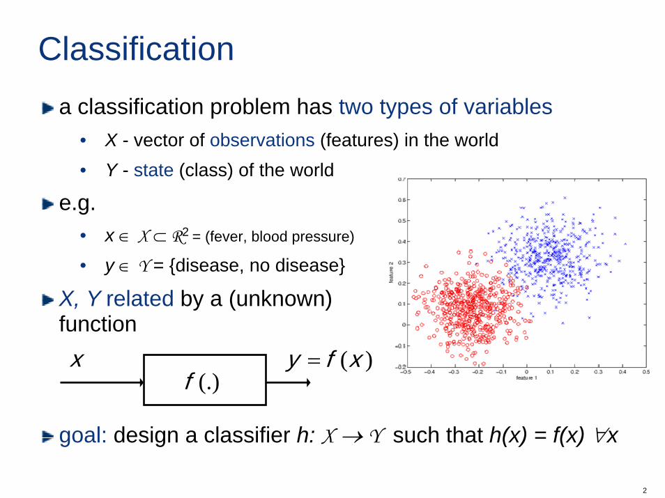
Classificationa classification problem has two types of variables

• X - vector of observations (features) in the world• Y - state (class) of the world

e.g. • x ∈ X ⊂ R2 = (fever, blood pressure)

• y ∈ Y = disease, no disease

X, Y related by a (unknown) function

goal: design a classifier h: X → Y such that h(x) = f(x) ∀x

)(xfy =x(.)f

3

Linear classifier implements the decision rule

with

has the properties• it divides X into two “half-spaces”

• boundary is the plane with:• normal w• distance to the origin b/||w||

• g(x)/||w|| distance from x to boundary• for a linearly separable training set

D = (x1,y1), ..., (xn,yn) we have zero empirical risk when

bxwxg T +=)(⎩⎨⎧

=<−>

= sgn[g(x)] if

if

0)(10)(1

)(*xgxg

xh

w

wb

x

wxg )(

( ) ibxwy iT

i ∀>+ ,0

4

The marginis the distance from the boundaryto the closest point

there will be no error if it is strictlygreater than zero

note that this is ill-defined in the sense that γ does not change if both w and b are scaled by λwe need a normalization

( ) 0,0 >⇔∀>+ γ ibxwy iT

i

w

y=1

y=-1

w

wb

x

wxg )(

wbxw i

T

i

+= minγ

5

Normalizationa convenient normalization is tomake |g(x)| = 1 for the closest point, i.e.

under which

the SVM is the classifier that maximizes the margin under these constraints

w

y=1

y=-1

w

wb

x

wxg )(

1min ≡+bxw iT

i

w1

=γ

( ) ibxwyw iT

ibw∀≥+ tosubject 1min 2

,

6

The dual problemno duality gap, the dual problem is

once this is solved, the vector

is the normal to the maximum margin planeb* can be left a free parameter (false pos.vs misses) or set to

0

21max

0

=⎭⎬⎫

⎩⎨⎧

+−

∑

∑∑≥

i

i

tosubject

ii

ijTij

ijiji

y

xxyy

α

αααα

∑=i

iii xyw α*

1/||w*||

1/||w*||

x

2)(*

−+ +−=

xxwbT

7

Support vectors

αi=0

αi=0

αi>0

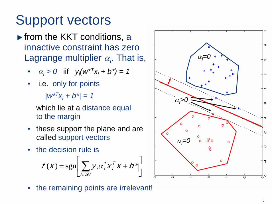
from the KKT conditions, a innactive constraint has zero Lagrange multiplier αi. That is, • αi > 0 iif yi(w*Txi + b*) = 1• i.e. only for points

|w*Txi + b*| = 1 which lie at a distance equal to the margin

• these support the plane and are called support vectors

• the decision rule is

• the remaining points are irrelevant!

⎥⎦

⎤⎢⎣

⎡+= ∑

∈

*sgn)( * bxxyxfSVi

Tiiiα

8

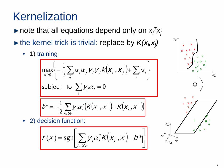
Kernelizationnote that all equations depend only on xi

Txj

the kernel trick is trivial: replace by K(xi,xj)• 1) training

• 2) decision function:

xx

x

x

x

xxx

xx

xx

oo

o

o

ooo

o

oooo

x1

x2

xx

x

x

x

xxx

xx

xx

oo

o

o

ooo

o

oooo

x1

x3x2

xn

Φ

( )

0

,21max

0

=⎭⎬⎫

⎩⎨⎧

+−

∑

∑∑≥

i

i

tosubject

ii

ijijij

iji

y

xxkyy

α

αααα

( ) ( )( )−+

∈

+−= ∑ xxKxxKyb iiiSVi

i ,,21* *α

( ) ⎥⎦

⎤⎢⎣

⎡+= ∑

∈

*,sgn)( * bxxKyxfSVi

iiiα

9

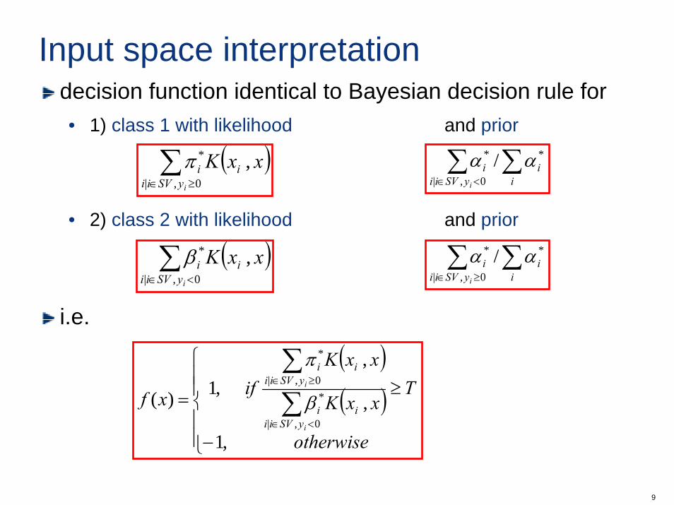
Input space interpretationdecision function identical to Bayesian decision rule for• 1) class 1 with likelihood and prior

• 2) class 2 with likelihood and prior

i.e.

( )∑≥∈ 0,|

* ,iySVii

ii xxKπ ∑∑<∈ i

iySVii

ii

*

0,|

* / αα

( )∑<∈ 0,|

* ,iySVii

ii xxKβ ∑∑≥∈ i

iySVii

ii

*

0,|

* / αα

( )( )

⎪⎪⎩

⎪⎪⎨

⎧

−

≥= ∑∑

<∈

≥∈

otherwise

TxxK

xxKifxf

i

i

ySViiii

ySViiii

,1

,

,,1)(

0,|

*0,|

*

β

π

10

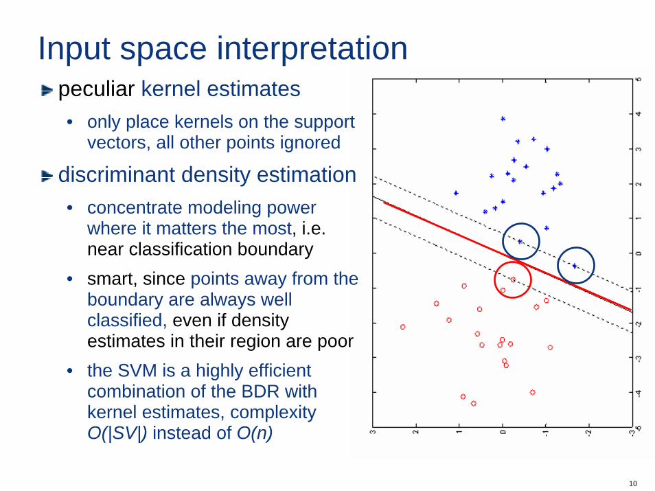
Input space interpretationpeculiar kernel estimates• only place kernels on the support

vectors, all other points ignored

discriminant density estimation• concentrate modeling power

where it matters the most, i.e. near classification boundary

• smart, since points away from the boundary are always well classified, even if density estimates in their region are poor

• the SVM is a highly efficient combination of the BDR with kernel estimates, complexity O(|SV|) instead of O(n)

11

Limitations of the SVMappealing, but also points outthe limitations of the SVM:• major problem of kernel density

estimation is the choice ofbandwidth

• if too small estimates have toomuch variance, if too large theestimates have too much bias

• this problem appears again forthe SVM

• no generic “optimal” procedure tofind the kernel or its parameters

• requires trial and error• note, however, that this is less of

a headache since only a few kernels have to be evaluated

12

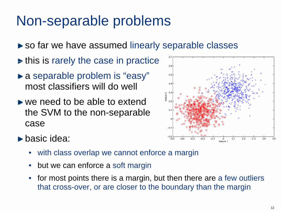
Non-separable problemsso far we have assumed linearly separable classesthis is rarely the case in practicea separable problem is “easy”most classifiers will do wellwe need to be able to extendthe SVM to the non-separablecasebasic idea:• with class overlap we cannot enforce a margin• but we can enforce a soft margin• for most points there is a margin, but then there are a few outliers

that cross-over, or are closer to the boundary than the margin

13

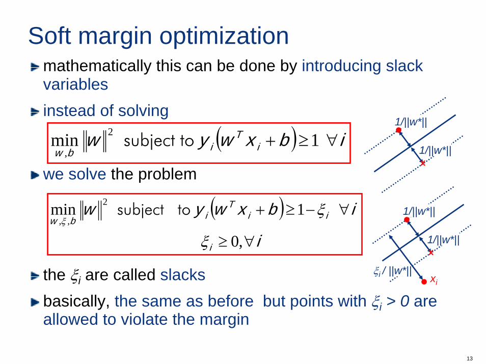
Soft margin optimizationmathematically this can be done by introducing slack variablesinstead of solving

we solve the problem

the ξi are called slacksbasically, the same as before but points with ξi > 0 are allowed to violate the margin

( ) ibxwyw iT

ibw∀≥+ tosubject 1min 2

,

( )i

ibxwyw

i

iiT

ibw

∀≥

∀−≥+

,0

1min 2

,,

ξ

ξξ

tosubject

1/||w*||

1/||w*||

x

ξi / ||w*||xi

1/||w*||

1/||w*||

x

14

Soft margin optimizationnote that the problem is not really well definedby making ξi arbitrarily large, any w will dowe need to penalize large ξi

this is done by solving instead

f(ξ) is usually a norm. We consider• the 1-norm: the 2-norm:

( )i

ibxwy

Cfw

i

iiT

i

bw

∀≥∀−≥+

+

,01

)(min 2

,,

ξξ

ξξ

tosubject

1/||w*||

1/||w*||

x

ξi / ||w*||xi

∑=i

if ξξ )( ∑=i

if 2)( ξξ

15

2-norm SVM

note that • if ξi < 0, and the constraint (**) is satisfied then• (**) is satisfied by ξi = 0 and the cost will be smaller• hence ξi < 0 is never a solution and the positivity constraints on

the ξi are redundant• they can therefore be dropped

( )i

ibxwy

Cw

i

iiT

i

iibw

∀≥∀−≥+

+ ∑

,0,1

min 22

,,

ξξ

ξξ

tosubject

(**)

16

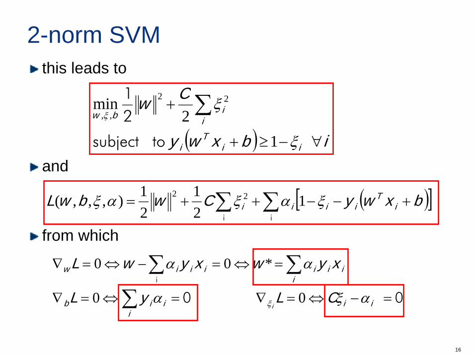
2-norm SVMthis leads to

and

from which

( ) ibxwy

Cw

iiT

i

iibw

∀−≥+

+ ∑ tosubject

21

ξ

ξξ

12

min 22

,,

0 0 i

=−⇔=∇=⇔=∇

=⇔=−⇔=∇

∑

∑∑ CLyL

xywxywL

iii

iib

iiiiiiiw

iαξα

αα

ξ 00

*00

( )[ ] ii

∑∑ +−−++= bxwyCwbwL iT

iiii ξαξαξ 121

21),,,( 22

17

2-norm dual problemplugging back we get the Lagrangian

Cyxyw ii

iii

iiii

αξαα === ∑∑ 0, ,*

( )

∑∑

∑∑∑

∑

∑∑∑∑

∑∑

+⎟⎟⎠

⎞⎜⎜⎝

⎛+−=

+⎟⎟⎠

⎞⎜⎜⎝

⎛+−=

=−

−+−=

⎥⎦⎤

⎢⎣⎡ +−−+⎟

⎠⎞

⎜⎝⎛+=

ii

ijj

Tij

ijiji

ii

iij

Tij

ijiji

iii

ijj

Tijijii

i

ij

Tij

ijiji

iT

ii

ii

i

Cxxyy

Cxxyy

by

xxyyC

xxyy

bxwyCC

CwrbwL

αδ

αα

αααα

α

αααααα

ααααξ

21

121

21

21

122

1),,,*,(

2

0

2

22

i

i

43421

⎩⎨⎧

≠=

=jiji

ij ,0,1

δ

18

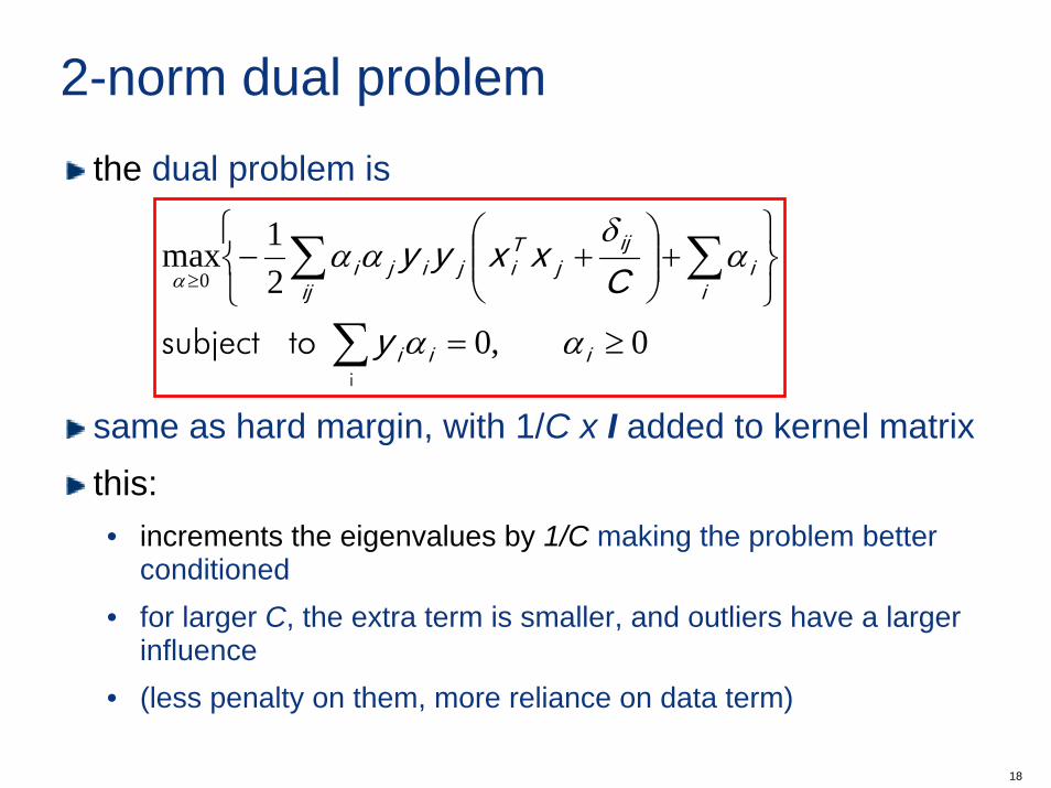
2-norm dual problemthe dual problem is

same as hard margin, with 1/C x I added to kernel matrixthis:• increments the eigenvalues by 1/C making the problem better

conditioned• for larger C, the extra term is smaller, and outliers have a larger

influence • (less penalty on them, more reliance on data term)

0,0

21max

0

≥=⎭⎬⎫

⎩⎨⎧

+⎟⎟⎠

⎞⎜⎜⎝

⎛+−

∑

∑∑≥

iii

ii

ijj

Tij

ijiji

y

Cxxyy

αα

αδ

ααα

tosubject i

19

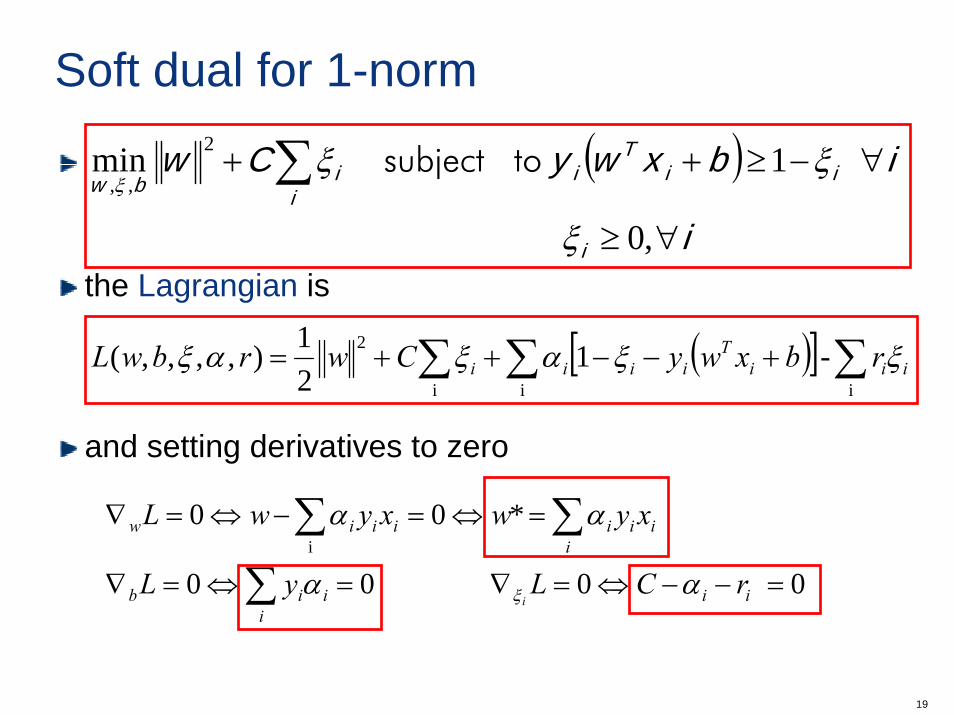
Soft dual for 1-norm

the Lagrangian is

and setting derivatives to zero

( )i

ibxwyCw

i

iiT

ii

ibw

∀≥

∀−≥++ ∑,0

1min 2

,,

ξ

ξξξ

tosubject

( )[ ] ∑∑∑ +−−++=iii

2 - 121),,,,( iii

Tiiii rbxwyCwrbwL ξξαξαξ

00 0 0

*00i

=−−⇔=∇=⇔=∇

=⇔=−⇔=∇

∑

∑∑ rCLyL

xywxywL

iii

iib

iiiiiiiw

iαα

αα

ξ

20

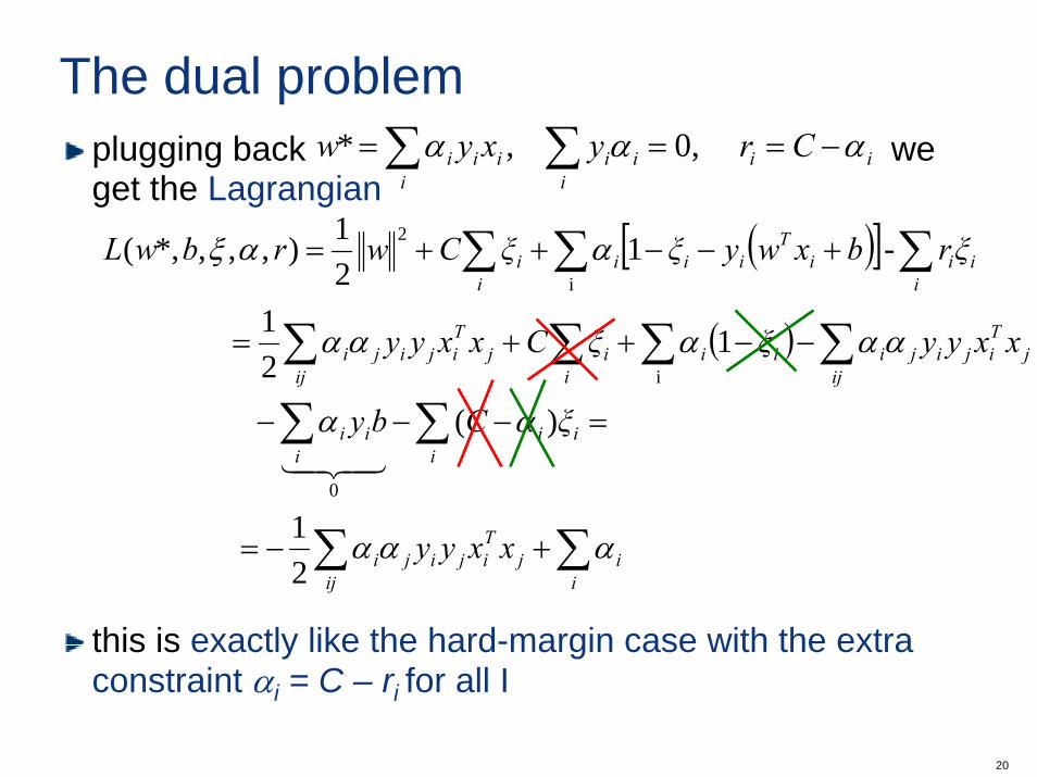
The dual problemplugging back we get the Lagrangian

this is exactly like the hard-margin case with the extra constraint αi = C – ri for all I

iii

iii

iii Cryxyw ααα −=== ∑∑ 0, ,*

( )[ ]

( )

∑∑

∑∑

∑∑∑∑

∑∑∑

+−=

=−−−

−−++=

+−−++=

iij

Tij

ijiji

iii

iii

ijjijiii

iij

Tij

ijiji

iiii

Tiii

ii

xxyy

ξCby

xyyξξCxxyy

ξrbxwyξξCwrbwL

ααα

αα

ααααα

ααξ

21

)(

121

- 121),,,*,(

0

i

i

2

43421

jTi x

21

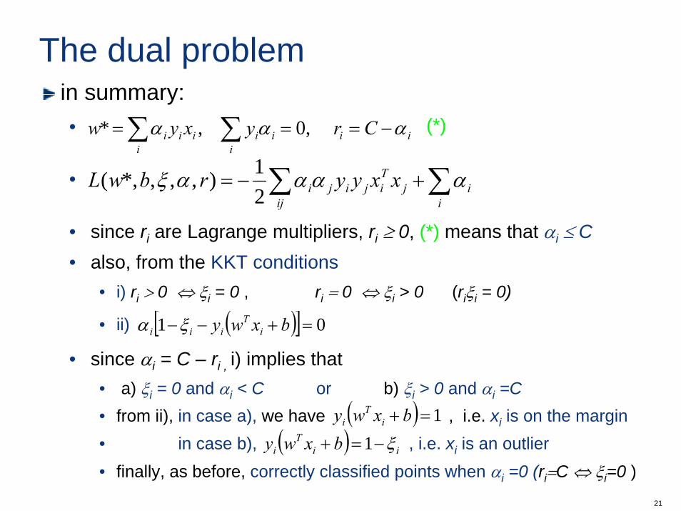
The dual problemin summary:•

•

• since ri are Lagrange multipliers, ri ≥ 0, (*) means that αi ≤ C• also, from the KKT conditions

• i) ri > 0 ⇔ ξi = 0 , ri = 0 ⇔ ξi > 0 (riξi = 0)

• ii)

• since αi = C – ri , i) implies that• a) ξi = 0 and αi < C or b) ξi > 0 and αi =C• from ii), in case a), we have , i.e. xi is on the margin• in case b), , i.e. xi is an outlier • finally, as before, correctly classified points when αi =0 (ri=C ⇔ ξi=0 )

iii

iii

iii Cryxyw ααα −=== ∑∑ 0, ,*

∑∑ +−=i

ijTij

ijiji xxyyrbwL ααααξ

21),,,*,(

(*)

( )[ ] 01 =+−− bxwy iT

iii ξα

( ) 1=+ bxwy iT

i

( ) iiT

i bxwy ξ−=+ 1

22

The dual problem

αi=0

αi=0

0 < αi < c

*

*

αi = c

overall, dual problem is

the only difference with respect to the hard margin case is the box constraint on the αi.geometrically we have this

C

y

xxyy

i

ii

ijTij

ijiji

≤≤

=⎭⎬⎫

⎩⎨⎧

+−

∑

∑∑≥

α

α

αααα

0

,0 tosubject

21max

i

i0

23

Support vectors

αi=0

αi=0

0 < αi < c

*

*

αi = c

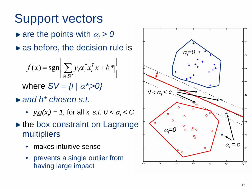
are the points with αi > 0as before, the decision rule is

where SV = i | α*i>0and b* chosen s.t.• yig(xi) = 1, for all xi s.t. 0 < αi < C

the box constraint on Lagrangemultipliers• makes intuitive sense• prevents a single outlier from

having large impact

⎥⎦

⎤⎢⎣

⎡+= ∑

∈

*sgn )( * bxxyxfSVi

Tiiiα

24

Soft margin SVMnote that C controls the importance of outliers• larger C implies that more emphasis is given to minimizing the

number of outliers• more of them will be within the margin

1-norm vs 2-norm• as usual, the 1-norm tends to limit more drastically the outlier

contributions• this makes it a bit more robust, and it tends to be used more

frequently in practice

common problem:• not really intuitive how to set up C• usually cross-validation, there is a need to cross-validate with

respect to both C and kernel parameters

25

υ-SVMa more recent formulation has been introduced to try to overcome this

advantages:• υ has intuitive interpretation:

• 1) υ is an upper bound on the proportion of training vectors that are margin errors, i.e. for which

• 2) υ is a lower bound on total number of support vectors

• more discussion on the homework

( )0,0

,

1min 2

,,,

≥∀≥∀−≥+

+− ∑

ρξξρ

ξυρρξ

tosubject

iibxwy

nw

i

iiT

i

iibw

ρ≤)( ii xgy

26

Connections to regularizationwe talked about penalizing functions that are too complicated, to improve generalizationinstead of the empirical risk, we should minimize the regularized risk

the SVM seems to be doing this in some sense:• it is designed to have as few errors as possible on training set

(this is controlled by the soft margin weight C)• we maximize the margin, by minimizing ||w||2 (which is a form of

complexity penalty)• hence, minimizing the margin must be connected to enforcing

some form of regularizer

[ ] [ ] [ ]ffRfR empreg Ω+= λ

27

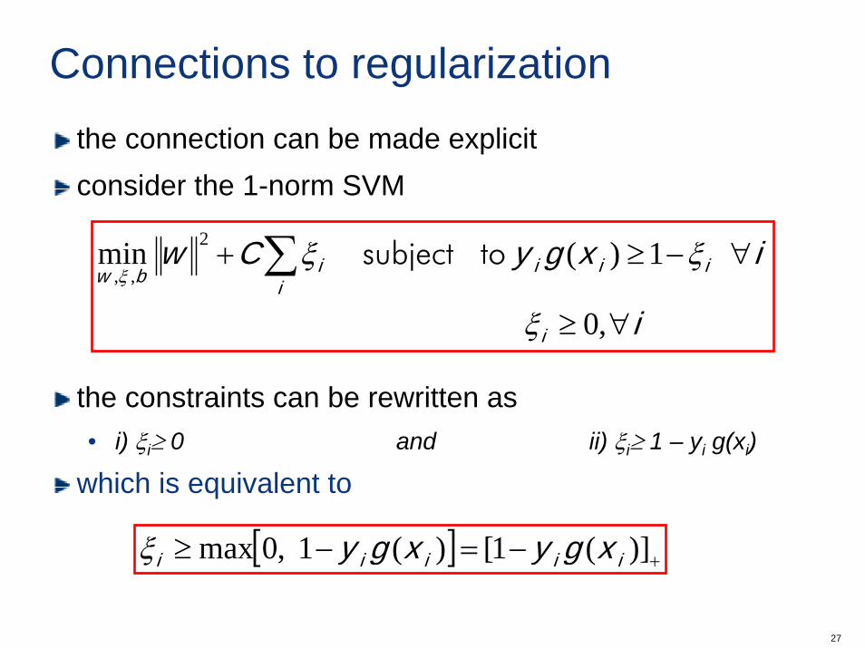
Connections to regularizationthe connection can be made explicitconsider the 1-norm SVM

the constraints can be rewritten as• i) ξi≥ 0 and ii) ξi≥ 1 – yi g(xi)

which is equivalent to

i

ixgyCw

i

iiii

ibw

∀≥

∀−≥+ ∑,0

1)(min 2

,,

ξ

ξξξ

tosubject

[ ] +−=−≥ )](1[)(1,0max iiiii xgyxgy ξ

28

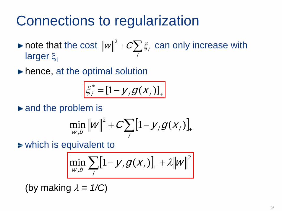
Connections to regularizationnote that the cost can only increase with larger ξi

hence, at the optimal solution

and the problem is

which is equivalent to

(by making λ = 1/C)

∑+i

iCw ξ2

+−= )](1[*iii xgyξ

[ ]∑ +−+i

iibwxgyCw )(1min 2

,

[ ] 2

,)(1min wxgy

iiibw

λ+−∑ +

29

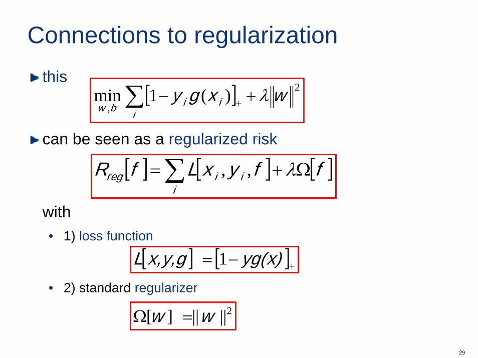
Connections to regularizationthis

can be seen as a regularized risk

with• 1) loss function

• 2) standard regularizer

[ ] 2

,)(1min wxgy

iiibw

λ+−∑ +

[ ] [ ] [ ]ffyxLfRi

iireg Ω+= ∑ λ,,

[ ] [ ]+−= yg(x)x,y,gL 1

2||||][ w w =Ω

30

The SVM lossit is interesting to compare the SVM loss

with the “0-1” loss:• the SVM loss penalizes large negative

margins• assigns some penalty to anything with

margin less than 1• for the “0-1” loss the errors are all

the same

the regularizer• penalizes planes of large w.• standard measure of complexity in regularization theory

[ ] [ ]+−= yg(x)x,y,gL 1

0 1

“0-1”

SVM loss

yg(x)

1

31

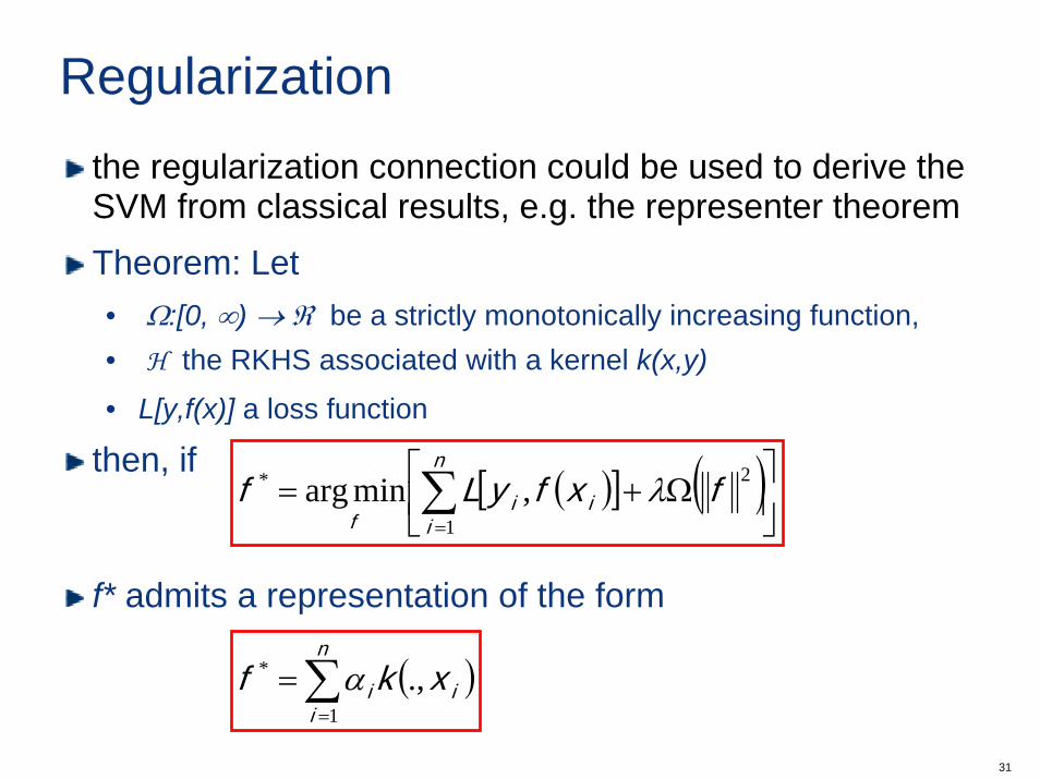
Regularizationthe regularization connection could be used to derive the SVM from classical results, e.g. the representer theoremTheorem: Let • Ω:[0, ∞) → ℜ be a strictly monotonically increasing function,• H the RKHS associated with a kernel k(x,y)

• L[y,f(x)] a loss function

then, if

f* admits a representation of the form

( )[ ] ( )⎥⎦

⎤⎢⎣

⎡Ω+= ∑

=

n

iii

ffxfyLf

1

2* ,minarg λ

( )∑=

=n

iii xkf

1

* .,α

32

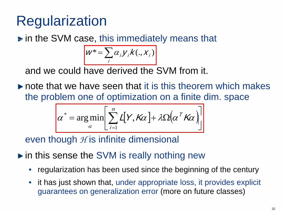
Regularizationin the SVM case, this immediately means that

and we could have derived the SVM from it.note that we have seen that it is this theorem which makes the problem one of optimization on a finite dim. space

even though H is infinite dimensional

in this sense the SVM is really nothing new• regularization has been used since the beginning of the century• it has just shown that, under appropriate loss, it provides explicit

guarantees on generalization error (more on future classes)

∑=i

iii xkyw )(.,* α

[ ] ( )⎥⎦

⎤⎢⎣

⎡Ω+= ∑

=

n

i

T KKYL1

* ,minarg ααλααα

33