Hard or Soft Classification?Large-Margin Unified Machines

Yufeng LIU, Hao Helen ZHANG, and Yichao WU

Margin-based classifiers have been popular in both machine learning and statistics for classification problems. Among numerous classifiers,some are hard classifiers while some are soft ones. Soft classifiers explicitly estimate the class conditional probabilities and then performclassification based on estimated probabilities. In contrast, hard classifiers directly target the classification decision boundary without pro-ducing the probability estimation. These two types of classifiers are based on different philosophies and each has its own merits. In thisarticle, we propose a novel family of large-margin classifiers, namely large-margin unified machines (LUMs), which covers a broad rangeof margin-based classifiers including both hard and soft ones. By offering a natural bridge from soft to hard classification, the LUM pro-vides a unified algorithm to fit various classifiers and hence a convenient platform to compare hard and soft classification. Both theoreticalconsistency and numerical performance of LUMs are explored. Our numerical study sheds some light on the choice between hard and softclassifiers in various classification problems.

KEY WORDS: Class probability estimation; DWD; Fisher consistency; Regularization; SVM.

1. INTRODUCTION

Classification is a very useful statistical tool for informationextraction from data. As a supervised learning technique, thegoal of classification is to construct a classification rule basedon a training set where both covariates and class labels aregiven. Once obtained, the classification rule can then be usedfor class prediction of new objects whose covariates are avail-able.

There is a large amount of literature on various classifi-cation methods, ranging from the very classical ones suchas Fisher linear discriminant analysis (LDA) and logistic re-gression (Hastie, Tibshirani, and Friedman 2001), to the re-cent machine learning based ones such as the Support Vec-tor Machine (SVM) (Boser, Guyon, and Vapnik 1992; Cortesand Vapnik 1995) and Boosting (Freund and Schapire 1997;Friedman, Hastie, and Tibshirani 2000). Among various clas-sification methods, there are two main groups of methods: softand hard classification. Our notions of soft and hard classifi-cation are the same as those defined in Wahba (1998, 2002).In particular, a soft classification rule generally estimates theclass conditional probabilities explicitly and then makes theclass prediction based on the largest estimated probability. Incontrast, hard classification bypasses the requirement of classprobability estimation and directly estimates the classifica-tion boundary. Typical soft classifiers include some traditionaldistribution-based likelihood approaches such as LDA and lo-gistic regression. On the other hand, some margin-based ap-proaches such as the SVM, generally distributional assumptionfree, belong to the class of hard classification methods.

Given a particular classification task, one natural question toask is that which type of classifiers should be used? Though a

Yufeng Liu is Associate Professor, Department of Statistics and OperationsResearch, Carolina Center for Genome Sciences, University of North Carolina,Chapel Hill, NC 27599 (E-mail: yfliu@email.unc.edu). Hao Helen Zhang isAssociate Professor and Yichao Wu is Assistant Professor, Department of Sta-tistics, North Carolina State University, Raleigh, NC 27695-8203. The authorsthank the editor, the associate editor, and three referees for their helpful sug-gestions that led to significant improvement of the article. The authors are par-tially supported by NSF grants DMS-0747575 (Liu), DMS-0645293 (Zhang)and DMS-0905561 (Wu), NIH grants NIH/NCI R01 CA-149569 (Liu and Wu),NIH/NCI P01 CA142538 (Liu and Zhang), and NIH/NCI R01 CA-085848(Zhang).

large number of classifiers are available, as it is typically thecase, there is no single method working best for all problems.The choice of classifiers really depends on the nature of thedataset and the primary learning goal. Wahba (2002) providedsome insights on soft versus hard classification. In particular,she demonstrated that the penalized logistic regression (PLR,Lin et al. 2000) and the SVM can both be fit into optimizationproblems in Reproducing Kernel Hilbert Spaces (RKHS). How-ever, the choice between the PLR and SVM for many practicalproblems is not clear. Recent rapid advances in high dimen-sional statistical data analysis also shed some light on this is-sue. With the large amount of high-dimension low-sample size(HDLSS) data available, effective statistical techniques for an-alyzing HDLSS data become more pressing. Traditional tech-niques such as LDA cannot even be computed directly whenthe dimension is larger than the sample size. Certain transfor-mation or dimension reduction is needed in order to apply LDA.Margin-based methods such as the SVM provide a totally dif-ferent view from the likelihood-based approaches. For example,the SVM does not have any distributional assumption and fo-cuses on the decision boundary only. It can be efficiently imple-mented for HDLSS data and has achieved great success in manyapplications (Vapnik 1998; Cristianini and Shawe-Taylor 2000;Schölkopf and Smola 2002). Recently, Marron, Todd, and Ahn(2007) pointed out that the SVM has the “data piling” phenom-ena in HDLSS settings due to its nondifferentiable hinge loss.In particular, when we project the training data onto the normvector of separating hyperplane for the linear SVM in high-dimensional problems, many projections are the same. Theyproposed a SVM variant, namely distance discriminant analysis(DWD), which does not have the data piling problem.

Between the two types of classifiers, soft classification pro-vides more information than hard classification and conse-quently it is desirable in certain situations where the probabilityinformation is useful. However, if the class probability functionis hard to estimate in some complicated problems, hard classi-fication may yield more accurate classifiers by targeting on the

© 2011 American Statistical AssociationJournal of the American Statistical Association

March 2011, Vol. 106, No. 493, Theory and MethodsDOI: 10.1198/jasa.2011.tm10319

166

Dow

nloa

ded

by [

66.2

6.70

.83]

at 2

0:12

06

Nov

embe

r 20

12

Liu, Zhang, and Wu: Hard or Soft Classification? Large-Margin Unified Machines 167

classification boundary only (Wang, Shen, and Liu 2008). Inpractice, it is difficult to choose between hard and soft classi-fiers, and consequently, it will be ideal to connect them sinceeach has its own strength. In this article, we propose a uni-fied framework of large-margin classifiers which covers a broadrange of methods from hard to soft classifiers. This new frame-work offers a unique transition from soft to hard classification.We call this family as Large-margin Unified Machines (LUMs).The proposed LUM family not only covers some well-knownlarge-margin classifiers such as the standard SVM and DWD, italso includes many new classifiers. One interesting example inthe LUM family is the new hybrid of SVM and Boosting.

One important contribution of the LUM is that it sheds somelight on the choice between hard and soft classifiers. Our inten-sive numerical study suggests that:

• soft classifiers tend to work better when the underlyingconditional class probability function is relatively smooth;or when the class signal level is relatively weak

• hard classifiers tend to work better when the underlyingconditional class probability function is relatively non-smooth; or when the two classes are close to be separable,that is, the class signal level is relatively strong; or whenthe dimension is relatively large compared to the samplesize.

Certainly, our observations may not be valid for all classifica-tion problems. Nevertheless, the LUM family provides a con-venient platform for deep investigation of the nature of a clas-sification problem. We propose an efficient tuning procedurefor the LUMs, and the resulting tuned LUM is shown to givenear-optimal classification performance compared with variousclassifiers in the LUM family. Thus we recommend it as a com-petitive classifier. Furthermore, we develop probability estima-tion techniques for the LUM family including hard classifierssuch as the SVM. The probability estimation method using therefitted LUM provides very competitive probability estimationfor both soft and hard classifiers in the LUM family.

Another major advantage of the LUM is its unified computa-tional strategies for different classifiers in the family. In prac-tice, different methods are often implemented with differentmethod-specific algorithms. For example, the SVM is typicallyfitted via solving a quadratic programming problem. The DWDwas proposed to be computed using the second-order cone pro-gramming (Marron, Todd, and Ahn 2007). For Boosting in theclassification setting, it can be implemented using the AdaBoostalgorithm (Freund and Schapire 1997). In this article, a uni-fied computational algorithm is developed for the LUMs tosolve seemingly very different methods in the family such asthe SVM and DWD. This greatly facilitates the implementationand comparison of various classifiers on a given problem. Wefurther propose a simple gradient descent algorithm to handlehigh-dimensional problems.

The remaining of the article is organized as follows. Sec-tion 2 introduces the proposed LUM methodology and dis-cusses some interesting special cases. Section 3 tackles the is-sues of Fisher consistency and class probability estimation. Sec-tion 4 addresses the computational aspect of LUMs. Section 5includes intensive simulated examples to demonstrate the per-formance of LUMs. Section 6 discusses two real data examples.Section 7 gives some final discussions. The Appendix containsthe technical proofs.

2. THE LUM METHODOLOGY

In supervised learning, we are given a training sample{(xi, yi); i = 1,2, . . . ,n}, distributed according to some un-known probability distribution P(x, y). Here, xi ∈ S ⊂ R

d andyi denote the input vector and output variable respectively, n isthe sample size, and d is the dimensionality of S . Consider atwo-class problem with y ∈ {±1} and let p(x) = P(Y = 1|X =x) be the conditional probability of class 1 given X = x. Letφ(x) : R

d → {±1} be a classifier and Cyφ(x) represent the costof misclassifying input x of class y into class φ(x). We setCyφ(x) = 0 if φ(x) = y and Cyφ(x) > 0 otherwise. One impor-tant goal of classification is to obtain a classifier φ(x) whichcan deliver the best classification accuracy. Equivalently, weaim to estimate the Bayes rule, φB(x), minimizing the general-ization error (GE), Err(φ) = E[CYφ(X)]. When equal costs areused with Cjl = 1; ∀j �= l, the Bayes rule can be reduced toφB(x) = sign(p(x) − 1/2).

The focus of this article is on large-margin classifiers. Amongvarious margin-based methods, the SVM is perhaps the mostwell known. While the SVM was first invented in the machinelearning community, it overlaps with classical statistics prob-lems, such as nonparametric regression and classification. It isnow known that the SVM can be fit in the regularization frame-work of Loss + Penalty using the hinge loss (Wahba 1998).In the regularization framework, the loss function is used tokeep the fidelity of the resulting model to the data. The penaltyterm in regularization helps to avoid overfitting of the resultingmodel. Specifically, margin-based classifiers try to calculate afunction f (x), a map from S to R, and use sign(f (x)) as the clas-sification rule. By definition of the classification rule, it is clearthat sign(yf (x)) reflects the classification result on the point(x, y). Correct classification occurs if and only if yf (x) > 0.The quantity yf (x) is commonly referred as the functional mar-gin and it plays a critical role in large-margin classificationtechniques. In short, the regularization formulation of binarylarge-margin classifiers can be summarized as the following op-timization problem:

minf

λJ(f ) + 1

n

n∑i=1

V(yif (xi)), (1)

where the minimization is taken over some function class F ,J(f ) is the regularization term, λ > 0 is a tuning parameter, andV(·) is a loss function. For example, the SVM uses the hingeloss function V(u) = [1 − u]+, where (u)+ = u if u ≥ 0 and 0otherwise.

Besides the SVM, many other classification techniques canbe fit into the regularization framework, for example, the PLR(Lin et al. 2000), the AdaBoost in Boosting (Freund andSchapire 1997; Friedman, Hastie, and Tibshirani 2000), the im-port vector machine (IVM; Zhu and Hastie 2005), ψ -learning(Shen et al. 2003; Liu and Shen 2006), the robust SVM (RSVM,Wu and Liu 2007), and the DWD (Marron, Todd, and Ahn2007).

Among various large margin classifiers, some are hard clas-sifiers which only focus on estimating the decision bound-ary. The SVM is a typical example of hard classifiers (Wang,Shen, and Liu 2008). In contrast to hard classifiers, soft clas-sifiers estimate the class conditional probability and the deci-sion boundary simultaneously. For example, the PLR and the

Dow

nloa

ded

by [

66.2

6.70

.83]

at 2

0:12

06

Nov

embe

r 20

12

168 Journal of the American Statistical Association, March 2011

Figure 1. Plots of LUM loss functions. Left panel: a = 1,c = 0,1,5,∞; Right panel: c = 0, a = 1,5,10,∞. The online versionof this figure is in color.

AdaBoost can be classified as soft classifiers (Zhang 2004;Tewari and Bartlett 2005). One may wonder which one is morepreferable, hard or soft classification? The answer truly dependson the problem given. In this article, we propose a family oflarge-margin classifiers which covers a spectrum of classifiersfrom soft to hard ones. In particular, for given a > 0 and c ≥ 0,define the following family of new loss functions

V(u) =

⎧⎪⎪⎨⎪⎪⎩

1 − u if u <c

1 + c1

1 + c

(a

(1 + c)u − c + a

)a

if u ≥ c

1 + c.

(2)

Note that V(u) in (2) has two different pieces, one for u <c

1+c and one for u ≥ c1+c , which are smoothly joined together at

c1+c . When u < c/(1 + c), V(u) is same as the hinge loss, [1 −u]+. Note that the hinge loss is not differentiable at u = 1, whileV(u) is differentiable for ∀u. Figure 1 displays several LUMloss functions for different values of a and c. As we can seefrom Figure 1, a and c play different roles in the loss function:c controls the connecting point between the two pieces of theloss as well as the shape of the right piece, and a determinesthe decaying speed for the right piece. We next show that theLUM is a very rich family, and in particular, it includes severalwell-known classifiers as special cases.

2.1 a > 0 and c → ∞: The Standard SVM

As pointed out before, the parameter c specifies the locationof the connection point of the two pieces of V(u) in (2). Theconnection point u = c/(1 + c) is between 0 and 1. As c in-creases, the connection point approaches 1 and the value V(u)

for u > c/(1+ c) becomes 0 when c → ∞. Thus, the hinge lossof the SVM becomes a limiting case in the LUM family. Thisis also reflected in Figure 1.

2.2 a = 1 and c = 1: DWD

Marron, Todd, and Ahn (2007) pointed out that for HDLSSdata, the SVM may suffer from “data piling” at the marginwhich may reduce generalizability. To solve the problem, theyproposed a different classifier, namely DWD. The idea wasmotivated from the maximum separation idea of the SVM. Inparticular, the SVM tries to separate the two classes as muchas possible without taking into account of correctly classifiedpoints far away from the boundary. Marron, Todd, and Ahn(2007) argued that this property of the SVM can result in the

“data piling” problem in HDLSS data. The method of DWDmodifies the SVM by allowing all points to influence the solu-tion. It gives high significance to those points that are close tothe hyperplane, with little impact from correct points that arefurther away. Recently, Qiao et al. (2010) proposed weightedDWD, as an extension of the standard DWD.

Despite its interesting connection with the SVM, the originalDWD proposal is not in the typical form Loss + Penalty of reg-ularization. In this section, we show that DWD is a special caseof the LUM family which corresponds to the LUM loss witha = 1 and c = 1. This result can help us to further understandDWD in the regularization prospective.

For simplicity, consider f (x) = w′x + b. The original DWDproposed by Marron, Todd, and Ahn (2007) solves the follow-ing optimization problem

minγ ,w,b,ξ

∑i

(1/γi) + Cn∑

i=1

ξi

subject to γi = yif (xi) + ξi,w′w ≤ 1, (3)

γi ≥ 0, ξi ≥ 0,∀i.

Theorem 1 shows that the DWD is a special case of LUMswith a = 1 and c = 1. Consequently, it provides more insighton the property of the DWD.

Theorem 1. With a one-to-one correspondence between Cand λ, the DWD optimization problem in (3) is equivalent to

minw,b

V(yif (xi)) + λ

2wTw, (4)

where V is the LUM loss function with a = 1 and c = 1.

2.3 a → ∞ and Fixed c: Hybrid of SVM and AdaBoost

Boosting is one of the most important statistical learningideas in the past decade. It was originally proposed for classi-fication problems by Freund and Schapire (1997) and has beenextended to many other areas in statistics. The idea of the orig-inal boosting algorithm AdaBoost is to apply the weak clas-sification algorithm sequentially to weighted versions of thedata. Then weak classifiers are combined to produce a strongone. Friedman, Hastie, and Tibshirani (2000) showed that theAdaBoost algorithm is equivalent to forward stagewise additivemodeling using the exponential loss function V(u) = exp(−u).

It turns out that the special case of the LUM family with a →∞ and any fixed c ≥ 0 has a very interesting connection to theexponential loss. For any given c ≥ 0, let a → ∞, then V(u)

becomes

V(u) =

⎧⎪⎪⎨⎪⎪⎩

1 − u if u <c

1 + c1

(1 + c)exp

{−[(1 + c)u − c]} if u ≥ c

1 + c.

(5)

In particular, when c = 0, then V(u) = 1 − u for u < 0 and e−u

otherwise, leading to the combination of the hinge loss and ex-ponential loss. As a result, this limiting case of the LUM lossfunction can be viewed as a hybrid of the standard SVM andthe AdaBoost.

The left panel of Figure 2 displays the hinge loss, the ex-ponential loss, and the LUM loss with a → ∞ and c = 0 as a

Dow

nloa

ded

by [

66.2

6.70

.83]

at 2

0:12

06

Nov

embe

r 20

12

Liu, Zhang, and Wu: Hard or Soft Classification? Large-Margin Unified Machines 169

Figure 2. Left Panel: Plot of a hybrid loss of the hinge loss and theexponential loss with c = 0; Right Panel: Plot of the hybrid loss withc = 0 versus the logistic loss. The online version of this figure is incolor.

hybrid loss of the two well-known loss functions. Interestingly,the hybrid loss makes use of the exponential loss for the rightside, consequently, all correctly classified points in the train-ing data can influence the decision boundary. The hinge loss,in contrast, does not make use of the data information once itsfunctional margin is larger than 1. For the left side of the hybridloss, it uses the hinge loss which is much smaller and thus muchcloser to the 0–1 loss function. This can yield robustness of theresulting classifiers when there are outliers in the data.

The hybrid loss with c = 0 also has an interesting connectionwith the logistic loss V(u) = log(1 + exp(−u)). Note that whenu gets large, the logistic loss and exponential loss are very closewith limu→∞(log(1 + exp(−u)))/(exp(−u)) = 1. When u be-comes negative and gets sufficiently small, log(1 + exp(−u)) isapproximately −u and differs from the hinge loss by 1. Thus,the hybrid loss with c = 0 lies between the logistic loss log(1 +exp(−u)) and the logistic loss+1, that is, 1+ log(1+exp(−u)).This relationship can be visualized from the right panel of Fig-ure 2. As shown in the plot, the right side of this hybrid lossbehaves like the logistic loss when u gets sufficiently large. Atthe same time, the left side of the hybrid loss is approximatelythe same as the logistic loss + 1. The main difference comesfrom the region of u around 0, where the hybrid loss penalizesthe wrong classified points around the boundary more severelythan the logistic loss. This difference may help the hybrid lossdeliver better performance than the logistic loss in certain situ-ations as shown in our simulation study in Section 5.

In Section 3, we will further study the aspect of class prob-ability estimation of various loss functions in the LUM family,which can provide more insight on the behaviors of differentloss functions.

3. FISHER CONSISTENCY ANDPROBABILITY ESTIMATION

To gain further theoretical insight about LUMs, we study thestatistical properties of the population minimizers of the LUMloss functions in this section. Since LUMs include both hardand soft classification rules as special cases, we will study itsproperties from two perspectives: the first one is its classifica-tion consistency, and the second one is to investigate whetherand when LUMs can estimate the class conditional probability.As we will show, the unique framework of LUMs enables us tosee how soft classifiers gradually become hard classifiers as theloss function changes.

Fisher consistency for a binary classification procedure basedon a loss function can be defined to be that the population min-imizer of the loss function has the same sign as p(x) − 1/2(Lin 2004). In our context, Fisher consistency requires thatthe minimizer of E[V(Yf (X))|X = x] has the same sign asp(x) − 1/2. Fisher consistency is also known as classificationcalibrated (Bartlett, Jordan, and McAuliffe 2006) and is a de-sirable property for a loss function. The following propositionimplies Fisher consistency of LUMs.

Proposition 1. Denote p(x) = P(Y = 1|X = x). For a givenX = x, the theoretical minimizer f ∗(x) of E[V(Yf (X))] is asfollows:

f ∗(x) =

⎧⎪⎪⎪⎪⎪⎪⎪⎨⎪⎪⎪⎪⎪⎪⎪⎩

− 1

1 + c(R(x)−1a − a + c) if 0 ≤ p(x) < 1/2[

− c

1 + c,

c

1 + c

]if p(x) = 1/2

1

1 + c(R(x)a − a + c) if 1/2 < p(x) ≤ 1,

(6)

where R(x) = [p(x)/(1 − p(x))](1/(a+1)).

The proof follows from the first derivative of the loss functionand the details are included in the Appendix. One immediateconclusion we can draw from Proposition 1 is that the class ofLUM loss functions is Fisher consistent.

As a remark, for c → ∞, the LUM loss V(yf (x)) reduces tothe hinge loss for the SVM with the corresponding minimizeras follows:

f ∗(x) =⎧⎨⎩

−1 if 0 ≤ p(x) < 1/2

(−1,1) if p(x) = 1/2

1 if 1/2 < p(x) ≤ 1.

As a result, the hinge loss is Fisher consistent for binary clas-sification as previously noted by Lin (2002). Moreover, we em-phasize that the SVM only estimates the classification bound-ary {x : p(x) = 1/2} without estimating p(x) itself (Wang, Shen,and Liu 2008). Thus, the LUM family becomes hard classifiersas c → ∞.

For a → ∞, the loss V(yf (x)) reduces to the hybrid loss ofthe hinge loss and the exponential loss, as shown in Section 2.3.Its corresponding minimizer is as follows:

f ∗(x) =

⎧⎪⎪⎪⎪⎪⎪⎪⎪⎪⎪⎪⎨⎪⎪⎪⎪⎪⎪⎪⎪⎪⎪⎪⎩

1

1 + c

[ln

(p(x)/(1 − p(x))

) − c]

if 0 ≤ p(x) < 1/2[− c

1 + c,

c

1 + c

]if p(x) = 1/2

1

1 + c

[ln

(p(x)/(1 − p(x))

) + c]

if 1/2 < p(x) ≤ 1.

(7)

From the minimizer f ∗(x) of V(yf (x)) in (6) with any finitec ≥ 0, we can convert the corresponding probabilities p(x) as

Dow

nloa

ded

by [

66.2

6.70

.83]

at 2

0:12

06

Nov

embe

r 20

12

170 Journal of the American Statistical Association, March 2011

Figure 3. Plot of the correspondence between f ∗(x) and p(x) asgiven in (8) with a = 1 and c = 0,1, and ∞. The online version of thisfigure is in color.

follows:

p(x) =

⎧⎪⎪⎪⎪⎪⎪⎪⎪⎪⎪⎪⎪⎪⎪⎪⎪⎨⎪⎪⎪⎪⎪⎪⎪⎪⎪⎪⎪⎪⎪⎪⎪⎪⎩

[1 +

[1

a{−(1 + c)f ∗(x) + a − c}

]a+1]−1

if f ∗(x) < − c

1 + c1

2if f ∗(x) ∈

[− c

1 + c,

c

1 + c

]

1 −[

1 +[

1

a{(1 + c)f ∗(x) + a − c}

]a+1]−1

if f ∗(x) >c

1 + c.

(8)

In order to estimate p(x), c needs to be finite. Interestingly,when p(x) = 1/2, p(x) and f ∗(x) do not have a one-to-onecorrespondence for any c > 0. In fact, all values of f ∗(x) ∈[− c

1+c ,c

1+c ] correspond to p(x) = 1/2. Figure 3 displays therelationship between between f ∗(x) and p(x) with a = 1 andc = 0,1, and ∞. When c > 0, the flat region of p(x) versusf ∗(x) as shown in Figure 3 makes the estimation of p(x) moredifficult. Thus, in terms of class conditional probability estima-tion, LUM loss functions with c = 0 will be the best case sincewe have a one-to-one correspondence between p(x) and f ∗(x)

for ∀p(x) ∈ [0,1]. Another important point we want to makeis that although as c increases, the class probability estimationmay become more difficult, LUMs can still provide class prob-ability estimation, even for very large values of c. The only ex-ceptional case is c → ∞, then the method reduces to the stan-dard SVM whose minimizer cannot estimate p(x) as mentionedbefore. Therefore, unlike the SVM, LUMs can provide classprobability estimation for any finite c, although the estimationdeteriorates as c increases.

As a remark, we note that the relationship between f ∗(x)

and p(x) given in (6) and (8) can be cast as a link func-tion used in generalized linear models (GLM) (McCullaghand Nelder 1989), although LUMs and GLM were originatedfrom very different views. For example, the logistic regressionuses the logit link function log(p(x)/(1 − p(x)) = f (x) with

p(x) = exp(f (x))/(1 + exp(f (x))). Interestingly, this link func-tion matches the form of the minimizer of our hybrid loss givenin (7) with c = 0. This observation further confirms the softclassification behavior of the LUM family when c = 0.

Although the relationship between f ∗(x) and p(x) can helpus to obtain estimation of p(x), calculation of f (x) for an ac-curate classification boundary and estimation of p(x) have dif-ferent goals. Even if f (x) can yield an accurate classificationboundary, f (x) itself may not be accurate enough for the esti-mation of p(x) since the classification boundary only dependson sign(f (x)). This problem can be more severe if there is a lotof shrinkage on f (x) by the regularization term. To improve theprobability estimation accuracy, we consider a refitted LUM bycalculating a refined estimate associated with two parameters(γ0, γ1) as f (2)(x) = γ0 + γ1f (1)(x), where f (1)(x) is the solu-tion by the original LUM regularization problem (1). In partic-ular, with f (1) given, the refitted LUM solves an unregularizedproblem, with the same a as for f (1)(x) and c = 0 in the LUMloss, as follows:

minγ0,γ1

n∑i=1

V(yi

(γ0 + γ1f (1)(xi)

)). (9)

The idea is that f (2)(x) serves as a scaled-corrected version off (1)(x) for probability estimation. This can be very effective iff (1)(x) gives accurate classification boundary. Once f (2)(x) isobtained, we can use it to estimate p(x) via (8), with the samea as for f (1)(x) and c = 0. Here we use c = 0 in the refittingstep since the corresponding formula has a one-to-one corre-spondence between p(x) and f ∗(x). As shown in our simulatedexamples in Section 5, probability estimation using the refittedLUM often leads to great improvement over that of the originalLUM solution.

4. COMPUTATIONAL ALGORITHM

The LUM loss V(u) is convex and first-order differentiable,but it is not second-order differentiable. One can use variousconvex optimization tools to fit the LUMs, such as nonlinearoptimization functions in R and Matlab and specialized licensedoptimization solvers such as MOSEK and MINOS. All of thesework well when the dimensionality of data is not too large.Next, we propose a simple alternative algorithm for the LUMs,the coordinate gradient descent algorithm, which works effi-ciently for both low and high-dimensional data.

Now we present the coordinate descent algorithm to mini-mize the objective function of the LUMs

minf

λJ(f ) + 1

n

n∑i=1

V(yi(f (xi)), (10)

where J(f ) is the regularization function of the function f (·). Wefocus on linear learning with f (x) = x′w + b and J(f ) = 1

2 w′w.The extension to kernel learning is straightforward. Denote thesolution at the mth step by w(m) = (w(m)

1 , w(m)2 , . . . , w(m)

d )T and

b(m). At the (m + 1)th step, for j = 1,2, . . . ,d, define f (m+1)ij =∑

k<j xikw(m+1)k + ∑

k′>j xik′w(m)

k′ + b(m) and set

w(m+1)j = argmin

wj

λ

2w2

j + 1

n

n∑i=1

V(yi

(f (m+1)ij + xijwj

)). (11)

Dow

nloa

ded

by [

66.2

6.70

.83]

at 2

0:12

06

Nov

embe

r 20

12

Liu, Zhang, and Wu: Hard or Soft Classification? Large-Margin Unified Machines 171

Problem (11) involves a one-dimensional optimization and canbe solved using many routine optimization techniques such asthe Newton–Raphson method. Once finishing updating w(m+1)

jfor j = 1,2, . . . ,d, we update the intercept by setting

b(m+1) = argminb

n∑i=1

V

(yi

(b +

d∑j=1

xijw(m+1)j

)). (12)

We keep iterating until convergence. The convergence criterionwe used is to require ‖w(m) − w(m+1)‖2 + (b(m) − b(m+1))2 tobe sufficiently small.

5. SIMULATION

In this section, we use simulated examples to demonstratethe numerical performance of LUMs in various scenarios. Onemain advantage of the LUM is that it provides a convenient plat-form to fit a spectrum of large-margin classifiers, from soft tohard, using one common algorithm. This has greatly facilitateda systematic exploration and comparison of different types ofclassifiers. Moreover, the LUM produces the class probabilitiesas a by-product for each combination of a and c.

We consider five examples. The first example illustrates a sit-uation where soft classifiers outperform hard classifiers. Thesecond example shows a case that hard classifiers outperformsoft classifiers. The third example demonstrates the perfor-mance transition of hard and soft classifiers with varying sig-nal strength. The forth and fifth examples demonstrate how theperformance of LUMs changes when the data dimensionalityvaries. We fit the LUM classifiers with various choices of aand c. For each method, we generate a training set of size 100to fit the classifier, a validation set of size 100 to tune the reg-ularization parameters. For each pair (a, c), the correspondingtuning parameter λ is selected by minimizing the classificationerror over the validation set using a grid search.

For the purpose of classification, we fit the LUMs with dif-ferent combinations of (a, c) and report the probability estima-tion and classification results associated with each pair (a, c).In practice, a systematic tuning procedure is often desired toselect the optimal (a, c). Since two-dimensional tuning can betime consuming, we suggest a fast and effective tuning proce-dure for the LUMs. Our empirical experience with the LUMs

(shown later in five examples) as well as the loss shapes asshown in Figure 1 suggest that the classification performance ofthe LUMs is not quite sensitive to the choice of a, while c playsa more important role. The magnitude of c determines whetherthe classifier is soft or hard. For example, c = 0 yields a softclassifier and c = 10,000 gives a hard classifier. In light of this,we suggest to choose c from two extreme values {0;10,000}while fixing a at a constant value such as 1000. We call the re-sulting classifier the “tuned LUM,” which is computationallymore efficient than the exhaustive search over (a, c)-space. Insome sense, the “tuned LUM” tries to make a greedy choicebetween a pair of hard and soft classifiers, the two ends of theLUM family. Our numerical results show that the tuned LUMin general performs nearly as well as the LUM with the best(a, c). For the purpose of probability estimation, we comparethe probability estimation errors of the LUMs and the refittedLUMs described in Section 3.

For each classifier, we evaluate its performance in both clas-sification accuracy and probability estimation, respectively us-ing the classification error of the estimated classifier and themean absolute error (MAE) EX|p(X) − p(X)| of the estimatedconditional probability on the test set of size 100,000. For fur-ther comparison, we also report the results of the PLR. We con-duct 1000 replications for each method in all examples, andreport the average test errors, MAEs, and the associated MonteCarlo standard errors (SEs).

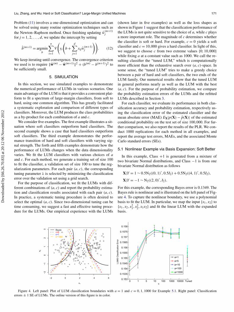
5.1 Nonlinear Example via Basis Expansion: Soft Better

In this example, Class +1 is generated from a mixture oftwo bivariate Normal distributions, and Class −1 is from onebivariate Normal distribution as follows

X|Y = 1 ∼ 0.5N2((0,1)′,0.5I2) + 0.5N2((4,1)′,0.5I2),

X|Y = −1 ∼ N2((2,0)′, I2).

For this example, the corresponding Bayes error is 0.1349. TheBayes rule is nonlinear and is illustrated on the left panel of Fig-ure 4. To capture the nonlinear boundary, we use a polynomialbasis to fit the LUM. In particular, we map the input {x1, x2} to{x1, x2, x2

1, x22, x1x2} and fit the linear LUM with the expanded

basis.

Figure 4. Left panel: Plot of LUM classification boundaries with a = 1 and c = 0,1,1000 for Example 5.1. Right panel: Classificationerrors ± 1 SE of LUMs. The online version of this figure is in color.

Dow

nloa

ded

by [

66.2

6.70

.83]

at 2

0:12

06

Nov

embe

r 20

12

172 Journal of the American Statistical Association, March 2011

There are two parameters a and c in the LUM function, andeach combination of them will result in a different classifier.As we pointed out before, a and c serve different roles in theLUM family of loss functions: c determines whether the cor-responding classifier is soft or hard, whereas a controls thedecaying speed of the loss function. We explore the effect ofa and c, via calculating the classifiers corresponding to vari-ous values of these parameters with a = 1,5,10,100,1000 andc = 0,1,5,10,100,1000,10,000. As c → ∞, the LUM classi-fier approaches to the SVM. Since the solutions barely changeafter c ≥ 1000, the LUM classifier with c ≥ 1000 can be viewedas a good approximation of the SVM classifier. Our limited nu-merical experience confirms that the LUM solution with largec and the SVM solution are almost identical.

The right panel of Figure 4 summarizes the average test clas-sification errors over 1000 repetitions for different values of aand c. It is seen that LUMs with c = 0 and 1 give the small-est test errors in all settings, suggesting that soft classificationoutperforms hard classification within the LUM family for thisexample. The effects of a appear to be very small. On the rightpanel of Figure 4, we also report the performance of the tunedLUM, denoted by “Tuned,” for each a. More explicitly the“tuned” LUM for each a is defined as follows. For each rep-etition and a fixed a, we apply another layer of tuning by com-paring the best tuning errors over the validation set for c = 0and c = 10,000 and the corresponding test error is given by thetest error for the LUM with c = 0 or c = 10,000 depending onwhich one gives a smaller tuning error. The performance of thetuned LUM method is close to the best among all LUMs withvarious a and c. For comparison, we also calculated the classi-fication accuracy of the PLR. The corresponding test error (SE)are 0.1563 (0.0005).

On the left panel of Figure 4, we depict the classificationboundaries given by the Bayes rule and various LUM classifierswith c = 0,1,10,1000, for one simulated dataset of size 200.As we can see from the plot, all LUMs are reasonably close tothe Bayes boundary, and the one corresponding to c = 0 is theclosest one to the Bayes rule.

Table 1 summarizes the MAEs for the estimated class proba-bilities over the 1000 repetitions. The LUM with c = 0 gives thesmallest MAE among all the LUM estimates, which is consis-tent to their theoretical properties studied previously. The differ-ences in MAEs between soft and hard LUMs are quite signifi-cant, in view of the SEs. Interestingly, the refitted LUMs largelyimprove probability estimation. Furthermore, the difference be-tween refitted soft and hard LUMs in terms of MAEs becomesmuch smaller than that of the original LUMs. The correspond-ing MAE (SE) for the PLR are 0.0957 (0.0012). Overall, we canconclude that LUMs yield competitive performance in terms ofboth classification accuracy and probability estimation.

5.2 Random Flipping Example: Hard Better

In this two-dimensional example, covariates X1 and X2 areindependently generated from Uniform[−1,1]. Conditional onX1 and X2, the class output is generated as follows: Y =sign(X1 + X2) when |X1 + X2| ≥ 0.5; when |X1 + X2| < 0.5,Y = sign(X1 + X2) with probability 0.8 and −sign(X1 + X2)

with probability 0.2.

Table 1. Average MAEs for probability estimation in Example 5.1.The corresponding SEs for the average LUM MAEs and average

refitted LUM MAEs range from 0.0008 to 0.0014 andfrom 0.0006 to 0.0007, respectively

a

c 1 5 10 100 1000

LUM MAEs0 0.0948 0.0955 0.0971 0.0983 0.09841 0.0982 0.1027 0.1035 0.1045 0.10445 0.1117 0.1145 0.1155 0.1164 0.1165

10 0.1185 0.1216 0.1219 0.1227 0.1226100 0.1276 0.1283 0.1286 0.1288 0.1287

1000 0.1289 0.1290 0.1292 0.1290 0.129110,000 0.1291 0.1292 0.1293 0.1290 0.1294

Refitted LUM MAEs0 0.0791 0.0782 0.0788 0.0795 0.07951 0.0780 0.0778 0.0783 0.0792 0.07925 0.0803 0.0796 0.0801 0.0807 0.0808

10 0.0811 0.0805 0.0808 0.0815 0.0816100 0.0807 0.0800 0.0806 0.0813 0.0813

1000 0.0807 0.0799 0.0804 0.0810 0.081210,000 0.0807 0.0801 0.0804 0.0811 0.0812

The underlying conditional class probability function of thisexample is a step function. Thus, in this case, class probabili-ties are difficult to estimate and the classification accuracy ofsoft classifiers may be sacrificed by probability estimation. Weexpect that hard classifiers, bypassing probability estimation,may work better than soft classifiers. The classification accu-racy results are shown in Figure 5.

Indeed, hard classifiers work much better in this examplein terms of classification accuracy. The tuned LUM works ex-tremely well here. The test error (SE) of the PLR are 0.1242(0.0005). Its performance is similar to that of the LUM withsmall c. Similar to Example 5.1, the classification performanceis not very sensitive to the choice of a.

The probability estimation results of LUMs are summarizedin terms of MAEs in Table 2. Since soft classifiers do not workwell for this example, we do not expect them to produce accu-rate probability estimation. Indeed, as shown in Table 2, prob-ability estimation of the original LUMs is not satisfactory. The

Figure 5. Classification results of LUMs for Example 5.2 with var-ious a and c. The online version of this figure is in color.

Dow

nloa

ded

by [

66.2

6.70

.83]

at 2

0:12

06

Nov

embe

r 20

12

Liu, Zhang, and Wu: Hard or Soft Classification? Large-Margin Unified Machines 173

Table 2. Probability MAEs of Example 5.2 given by LUMs. Thecorresponding SEs for the average LUM MAEs and average

refitted LUM MAEs range from 0.0027 to 0.0033 andfrom 0.0003 to 0.0008, respectively

a

c 1 5 10 100 1000

LUMS MAE0 0.2008 0.2030 0.2037 0.2055 0.20491 0.2068 0.2137 0.2142 0.2150 0.21535 0.2170 0.2200 0.2202 0.2212 0.2215

10 0.2190 0.2221 0.2218 0.2230 0.2230100 0.2176 0.2177 0.2178 0.2183 0.2183

1000 0.2172 0.2170 0.2173 0.2178 0.217810,000 0.2173 0.2174 0.2171 0.2175 0.2170Best 0.2061 0.2104 0.2107 0.2115 0.2114

Refitted LUMS MAE0 0.0814 0.0760 0.0753 0.0745 0.07471 0.0782 0.0746 0.0740 0.0736 0.07365 0.0782 0.0746 0.0741 0.0737 0.0736

10 0.0782 0.0746 0.0741 0.0736 0.0736100 0.0783 0.0746 0.0740 0.0736 0.0736

1000 0.0782 0.0746 0.0741 0.0736 0.073610,000 0.0782 0.0746 0.0740 0.0736 0.0736

refitted LUMs produce dramatic improvement over the origi-nal LUMs. Interestingly, the refitted LUMs with large c’s workeven slightly better than those with smaller c’s. This is con-sistent with the observation by Wang, Shen, and Liu (2008)that better classification can be translated into better probabil-ity estimation. In this case, the original LUMs provide accurateclassification boundaries and then the refitted LUMs correct thescales of the classification function by the original LUMs forbetter probability estimation. In this case, the MAE (SE) of thePLR are 0.1823 (0.003), much worse than our refitted LUMs.

5.3 Varying Signal Example: Transition BetweenHard and Soft Classifiers

In this two-dimensional example, predictors X1 and X2 areuniformly distributed over {(x1, x2) : |x1| + |x2| ≤ 2}. Condi-tional on X1 = x1 and X2 = x2, Y takes 1 with probabil-ity es(x1+x2)/(1 + es(x1+x2)) and −1 with probability 1/(1 +es(x1+x2)) for some s > 0. This is essentially a binomial exam-ple with s controlling the signal strength level. As the previous

examples have demonstrated that the effect of a on the classifi-cation error is very minimal, we fix a = 1000 in this example.The goal of the current example is to explore the performancepattern for different c as the signal level varies. Figure 6 plotsthe classification errors for different c and different signal lev-els.

As shown in Figure 6, LUMs with small c’s, that is, soft clas-sifiers, work better for the case of weak signals with s = 0.2 and0.6. As we increase the signal levels, all classifiers give more ac-curate classification results. However, hard classifiers becomemore and more competitive. When s = 0.6, LUMs with smalland large c’s outperform those with middle values of c. Oncethe signal level is relatively high with s = 0.7 and 1.5, hard clas-sifiers, that is, LUMs with large c’s, outperform soft classifiers.This example implies that which type of classifiers performsbetter is related to the signal strength contained in data. In thisparticular setup, soft classifiers tend to work better when thesignal is weak, and hard classifiers seem to work better in thecase of strong signals.

5.4 Increasing Dimension Example With NonsparseSignal: From Soft Better to Hard Better

For this example, the data are generated from a Gaussianmixture distribution: positive samples are from N(μd, Id) andnegative samples are from N(−μd, Id) with μd = (μ,μ, . . . ,

μ)T . The dimension d changes from 10, 50, 100, 200, to 400.Here μ controls the signal level. We choose μ as a function ofd such that the Bayes error is fixed at 22% for different dimen-sions.

The previous examples have demonstrated that the effect ofa on the classification error is very minimal, so we fix a = 1000in this example. We plot the classification errors in Figure 7 fordifferent dimensionality d. As we can see from Figure 7, whenthe dimension d = 10 and 50, LUMs with smaller c’s, that is,soft classifiers, yield the best performance. As the dimensionincreases to d = 100, LUMs with large c’s become relativelymore competitive. When the dimension equals to 400, LUMswith large c’s work the best. This indicates that hard classifierstend to work better in high-dimensional classification examples.

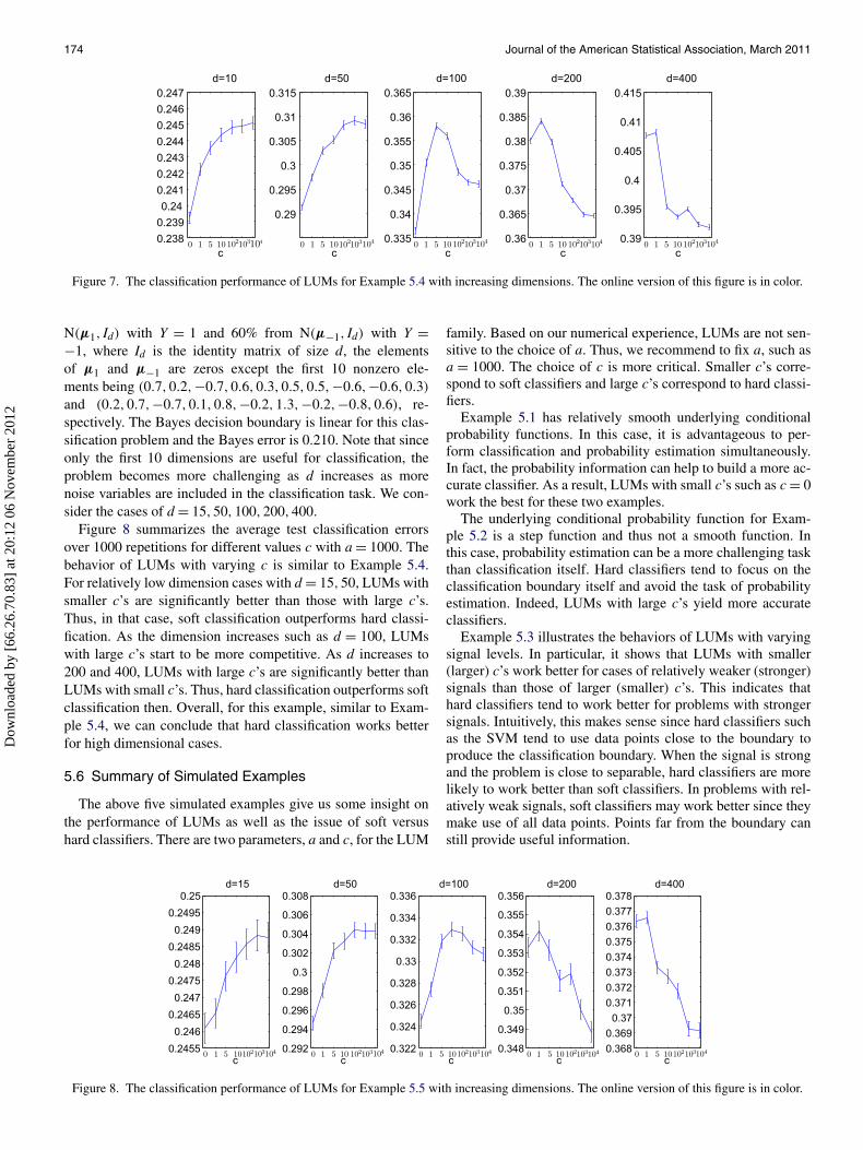
5.5 Increasing Dimension Example With Sparse Signal:From Soft Better to Hard Better

We generate the data as a mixture of two Gaussians in a15-dimensional space. In particular, 40% of data are from

Figure 6. The classification performance of LUMs for Example 5.3 with varying signal levels. The online version of this figure is in color.

Dow

nloa

ded

by [

66.2

6.70

.83]

at 2

0:12

06

Nov

embe

r 20

12

174 Journal of the American Statistical Association, March 2011

Figure 7. The classification performance of LUMs for Example 5.4 with increasing dimensions. The online version of this figure is in color.

N(μ1, Id) with Y = 1 and 60% from N(μ−1, Id) with Y =−1, where Id is the identity matrix of size d, the elementsof μ1 and μ−1 are zeros except the first 10 nonzero ele-ments being (0.7,0.2,−0.7,0.6,0.3,0.5,0.5,−0.6,−0.6,0.3)

and (0.2,0.7,−0.7,0.1,0.8,−0.2,1.3,−0.2,−0.8,0.6), re-spectively. The Bayes decision boundary is linear for this clas-sification problem and the Bayes error is 0.210. Note that sinceonly the first 10 dimensions are useful for classification, theproblem becomes more challenging as d increases as morenoise variables are included in the classification task. We con-sider the cases of d = 15,50,100,200,400.

Figure 8 summarizes the average test classification errorsover 1000 repetitions for different values c with a = 1000. Thebehavior of LUMs with varying c is similar to Example 5.4.For relatively low dimension cases with d = 15,50, LUMs withsmaller c’s are significantly better than those with large c’s.Thus, in that case, soft classification outperforms hard classi-fication. As the dimension increases such as d = 100, LUMswith large c’s start to be more competitive. As d increases to200 and 400, LUMs with large c’s are significantly better thanLUMs with small c’s. Thus, hard classification outperforms softclassification then. Overall, for this example, similar to Exam-ple 5.4, we can conclude that hard classification works betterfor high dimensional cases.

5.6 Summary of Simulated Examples

The above five simulated examples give us some insight onthe performance of LUMs as well as the issue of soft versushard classifiers. There are two parameters, a and c, for the LUM

family. Based on our numerical experience, LUMs are not sen-sitive to the choice of a. Thus, we recommend to fix a, such asa = 1000. The choice of c is more critical. Smaller c’s corre-spond to soft classifiers and large c’s correspond to hard classi-fiers.

Example 5.1 has relatively smooth underlying conditionalprobability functions. In this case, it is advantageous to per-form classification and probability estimation simultaneously.In fact, the probability information can help to build a more ac-curate classifier. As a result, LUMs with small c’s such as c = 0work the best for these two examples.

The underlying conditional probability function for Exam-ple 5.2 is a step function and thus not a smooth function. Inthis case, probability estimation can be a more challenging taskthan classification itself. Hard classifiers tend to focus on theclassification boundary itself and avoid the task of probabilityestimation. Indeed, LUMs with large c’s yield more accurateclassifiers.

Example 5.3 illustrates the behaviors of LUMs with varyingsignal levels. In particular, it shows that LUMs with smaller(larger) c’s work better for cases of relatively weaker (stronger)signals than those of larger (smaller) c’s. This indicates thathard classifiers tend to work better for problems with strongersignals. Intuitively, this makes sense since hard classifiers suchas the SVM tend to use data points close to the boundary toproduce the classification boundary. When the signal is strongand the problem is close to separable, hard classifiers are morelikely to work better than soft classifiers. In problems with rel-atively weak signals, soft classifiers may work better since theymake use of all data points. Points far from the boundary canstill provide useful information.

Figure 8. The classification performance of LUMs for Example 5.5 with increasing dimensions. The online version of this figure is in color.

Dow

nloa

ded

by [

66.2

6.70

.83]

at 2

0:12

06

Nov

embe

r 20

12

Liu, Zhang, and Wu: Hard or Soft Classification? Large-Margin Unified Machines 175

Examples 5.4 and 5.5 show how dimensionality of the classi-fication problem affects the choice between soft and hard clas-sifiers. The common belief in statistical learning is that hardclassifiers can be a good candidate for high-dimensional prob-lems. One potential reason is that data tend to be more separablein high-dimensional spaces, so hard classifiers may yield clas-sifiers with better generalization ability. Indeed, we can learnfrom Examples 5.4 and 5.5 that LUMs with large c’s becomemore competitive as the dimension increases.

Our numerical results suggest that our tuned LUMs betweenlarge and small c’s with a fixed a can yield near optimal classi-fication accuracy. For problems that we are uncertain about thechoice between soft and hard classifiers, we recommend to usethe tuned LUM.

In terms of probability estimation, LUMs with smaller c’syield much more accurate probability estimation than those oflarger c’s. The more interesting lesson is that the step of refittingcorrects the scale of the classification function and significantlyimproves the performance of probability estimation. It can beused as an attractive method of probability estimation for bothhard and soft classifiers.

6. REAL EXAMPLE

We apply the proposed LUMs to two real data exam-ples. The first example is the liver disorder dataset from theUCI benchmark repository. The dataset can be downloadedfrom http://www.ics.uci.edu/~mlearn/MLRepository.html. Thisdataset contains 345 observations and seven input features. Thefirst five features are all blood tests which are thought to be sen-sitive to liver disorders that might arise from excessive alcoholconsumption. The other two features are related to the mea-sure of alcoholic consumption per day. The goal of the problemis to use the blood test and alcoholic consumption informa-tion to classify the status of liver disorder. The second exampleis the lung cancer dataset, described in Liu et al. (2008). Thedataset contains 205 subjects including 128 adenocarcinoma,20 carcinoid, 21 squamous, 17 normal tissues, 13 colon cancermetastasis, and six small cell carcinoma samples. Since the ade-nocarcinoma class is the most heterogeneous class, we consider

the binary classification task of adenocarcinoma versus others.We select 200 genes with the most variation for classification.

Since there are no separate validation and testing data avail-able for these datasets, we randomly divide each dataset intothree parts: one part used as the training set, one part for tuning,and the third part used as the testing set. We repeat this process10 times and report the average test errors for linear LUMs inFigure 9.

The liver disorder example is shown to be a relatively diffi-cult classification problem with test errors over 30%. In view ofthe lesson we learn from Example 5.3, soft classification maywork better in this case. The left panel of Figure 9 shows thetest errors for various a and c. Again the effect of a is small,but it appears that smaller c works better, suggesting soft clas-sification is more preferable here. We also calculated the tunedLUMs. For a = 1000, the corresponding test error is 0.3470,which is near optimal compared to other errors in the plot.

The lung cancer example is a high-dimensional example andthe right panel of Figure 9 suggests that hard classificationworks better here. This is consistent with the findings in Exam-ples 5.4 and 5.5. In this case, the test error for the tuned LUMwith a = 1000 is 0.0957. Again this is near optimal in view ofthe test errors corresponding to various (a, c) reported in rightpanel of Figure 9.

7. DISCUSSION

Large-margin classifiers play an important role in classifica-tion problems. In this article, we propose a rich family calledthe LUM which covers a wide range of classifiers from soft tohard ones. The new family provides a natural bridge betweensoft and hard classification. Properties of this new family helpsto provide further insight on large-margin classifiers. Further-more, the LUM family includes some existing classifiers suchas the SVM and DWD as well as many new ones including thehybrid of the SVM and Boosting.

The LUM family is indexed by two parameters a and c. Ournumerical study shows that the performance of LUMs is notvery sensitive to the choice of a. Thus, we recommend to fix a atone value such as 1000. The role of c is more critical for the re-sulting classifier since it connects soft and hard classifiers. Our

Figure 9. Plots of classification errors by LUMs with various a and c. The liver disorder example and the lung cancer example are displayedon the left and right panels respectively. The online version of this figure is in color.

Dow

nloa

ded

by [

66.2

6.70

.83]

at 2

0:12

06

Nov

embe

r 20

12

176 Journal of the American Statistical Association, March 2011

numerical examples shed some light on the choice between softand hard classifiers. Furthermore, our tuned LUM, with fixed aand tuned c in {0;10,000}, appears to give near-optimal perfor-mance.

Our study on probability estimation shows that the step of re-fitting is critical. Moreover, our probability estimation schemeworks well for both hard and soft classifiers in the LUM fam-ily. As a result, it can also be used as a probability estimationtechnique for hard classifiers such as the SVM.

APPENDIX

Proof of Theorem 1

To simply the formulation (3), we remove γ and get the followingequivalent formulation of (3):

minw,b,ξ

∑i

1/(yif (xi) + ξi) + Cn∑

i=1

ξi

(A.1)subject to w′w ≤ 1, ξi ≥ 0,∀i.

To get the minimizer of (A.1), for fixed yif (xi), we first study the min-imizer of

A(ξi) ≡ 1

yif (xi) + ξi+ Cξi

with ξi ≥ 0. Note that

A′(ξi) = − 1

(yif (xi) + ξi)2

+ C.

• When yif (xi) ≤ 1/√

C, A′(ξi) < 0 if ξi < 1/√

C − yif (xi),A′(ξi) = 0 if ξi = 1/

√C − yif (xi), and A′(ξi) > 0 if ξi >

1/√

C − yif (xi). Then the minimizer ξ∗i = 1/

√C − yif (xi).

• When yif (xi) > 1/√

C, A′(ξi) > 0 for ∀ξi ≥ 0. Then ξ∗ = 0.

Then one can show that the optimization problem (A.1) is equivalentto the following problem:

minw,b

VCDWD(yif (xi)) subject to w′w ≤ 1, (A.2)

where VCDWD(u) = 2

√C − Cu if u ≤ 1/

√C and 1/u otherwise.

Let f = f√

C. Then we have VCDWD(yif (xi)) = √

CV1DWD(yif (xi)),

where V1DWD(u) = 2 − u if u ≤ 1 and 1/u otherwise. Then the opti-

mization problem (A.2) is equivalent to

minw,b

V1DWD(yif (xi)) subject to w′w ≤ C. (A.3)

Using Lagrange multiplier λ > 0, (A.3) can be written in the followingequivalent formulation

minw,b

V1DWD(yif (xi)) + λ

2w′w. (A.4)

From the convex optimization theory, we know that there is an one-to-

one correspondence between C in (A.3) and λ in (A.4). Denote ( ˆw,ˆb)

with given λ as the solution of (A.4). Then we have ˆw′ ˆw = C.Consider a = 1 and c = 1, then our loss V(u) = 1 − u if u ≤ 1/2

and 1/(4u) otherwise. Let u1 = 2u. Then V(u) = V1DWD(2u)/2 and

V1DWD(u1) = 2V(u1/2). Plugging the relationship into (A.4), we get

minw∗,b∗ V(yif

∗(xi)) + λ∗2

w∗′w∗, (A.5)

where f ∗ = f /2 and λ∗ = 2λ. Denote (w∗, b∗) with given λ∗ as the so-lution of (A.5). Then we have w∗′w∗ = ˆw′ ˆw/4 = C/4. Consequently,we can conclude that DWD is equivalent to LUM with a = 1 and c = 1.

Proof of Proposition 1

Notice E[V(Yf (X))] = E[E(V(Yf (X))|X = x)]. We can minimizeE[V(Yf (X))] by minimizing E(V(Yf (X))|X = x) for every x.

For any fixed x, E(V(Yf (X))|X = x) can be written as V(f (x))p(x)+V(−f (x))(1 − p(x)). For simplicity of notation, we drop x and need tominimize g(f ) = V(f )p + V(−f )(1 − p) with respect to f . To this end,we take the first order derivative of g(f ) since it is differentiable. Thenwe have

g′(f ) = pV ′(f ) − (1 − p)V ′(−f ), (A.6)

V ′(u) =

⎧⎪⎪⎨⎪⎪⎩

−1 if u <c

1 + c

−(

a

(1 + c)u − c + a

)a+1if u ≥ c

1 + c.

(A.7)

Plugging (A.7) into (A.6), we get

g′(f ) =

⎧⎪⎪⎪⎪⎪⎪⎪⎪⎪⎪⎪⎪⎪⎪⎪⎪⎪⎨⎪⎪⎪⎪⎪⎪⎪⎪⎪⎪⎪⎪⎪⎪⎪⎪⎪⎩

−p + (1 − p)

(a

(1 + c)(−f ) − c + a

)a+1

if f < − c

1 + c1 − 2p

if − c

1 + c≤ f ≤ c

1 + c

−p

(a

(1 + c)f − c + a

)a+1+ (1 − p)

if f >c

1 + c.

(A.8)

To obtain the minimizer of g(f ), we need to examine the signs ofits derivative g′(f ). When p < 1/2, g′(f ) > 0 for f ≥ − c

1+c and theminimizer f ∗ can be obtained by setting g′(f ) = 0 for f < − c

1+c . Sim-ilarly, when p > 1/2, g′(f ) < 0 for f ≤ c

1+c and the minimizer f ∗can be obtained by setting g′(f ) = 0 for f > c

1+c . When p = 1/2,g′(f ) < 0 for f < − c

1+c , g′(f ) > 0 for f > c1+c , and g′(f ) = 0 for

f ∈ [−c/(1 + c), c/(1 + c)]. The desired result then follows.

[Received May 2010. Revised October 2010.]

REFERENCES

Bartlett, P., Jordan, M., and McAuliffe, J. (2006), “Convexity, Classification,and Risk Bounds,” Journal of the American Statistical Association, 101,138–156. [169]

Boser, B., Guyon, I., and Vapnik, V. N. (1992), “A Training Algorithm for Op-timal Margin Classifiers,” The Fifth Annual Conference on ComputationalLearning Theory, Pittsburgh, PA: ACM Press, pp. 142–152. [166]

Cortes, C., and Vapnik, V. N. (1995), “Support-Vector Networks,” MachineLearning, 20, 273–279. [166]

Cristianini, N., and Shawe-Taylor, J. (2000), An Introduction to Support VectorMachines and Other Kernel-Based Learning Methods, Cambridge, UnitedKingdom: Cambridge University Press. [166]

Freund, Y., and Schapire, R. (1997), “A Decision Theoretic Generalization ofOn-Line Learning and an Application to Boosting,” Journal of Computerand System Sciences, 55, 119–139. [166-168]

Friedman, J. H., Hastie, T., and Tibshirani, R. (2000), “Additive Logistic Re-gression: A Statistical View of Boosting,” The Annals of Statistics, 28, 337–407. [166-168]

Hastie, T., Tibshirani, R., and Friedman, J. (2001), The Elements of StatisticalLearning: Data Mining, Inference, and Prediction, New York: Springer-Verlag. [166]

Lin, X., Wahba, G., Xiang, D., Gao, F., Klein, R., and Klein, B. (2000),“Smoothing Spline ANOVA Models for Large Data Sets With BernoulliObservations and the Randomized GACV,” The Annals of Statistics, 28,1570–1600. [166,167]

Lin, Y. (2002), “Support Vector Machines and the Bayes Rule in Classification,”Data Mining and Knowledge Discovery, 6, 259–275. [169]

(2004), “A Note on Margin-Based Loss Functions in Classification,”Statistics & Probability Letters, 68, 73–82. [169]

Liu, Y., and Shen, X. (2006), “Multicategory ψ -Learning,” Journal of the Amer-ican Statistical Association, 101, 500–509. [167]

Dow

nloa

ded

by [

66.2

6.70

.83]

at 2

0:12

06

Nov

embe

r 20

12

Liu, Zhang, and Wu: Hard or Soft Classification? Large-Margin Unified Machines 177

Liu, Y., Hayes, D. N., Nobel, A., and Marron, J. S. (2008), “Statistical Signif-icance of Clustering for High Dimension Low Sample Size Data,” Journalof the American Statistical Association, 103, 1281–1293. [175]

Marron, J. S., Todd, M., and Ahn, J. (2007), “Distance Weighted Discrimi-nation,” Journal of the American Statistical Association, 102, 1267–1271.[166-168]

McCullagh, P., and Nelder, J. (1989), Generalized Linear Models, London,United Kingdom: Chapman & Hall/CRC. [170]

Qiao, X., Zhang, H. H., Liu, Y., Todd, M. J., and Marron, J. S. (2010),“Weighted Distance Weighted Discrimination and Its Asymptotic Proper-ties,” Journal of the American Statistical Association, 105, 401–414. [168]

Schölkopf, B., and Smola, A. J. (2002), Learning With Kernels, Cambridge,MA: MIT Press. [166]

Shen, X., Tseng, G. C., Zhang, X., and Wong, W. H. (2003), “On ψ -Learning,”Journal of the American Statistical Association, 98, 724–734. [167]

Tewari, A., and Bartlett, P. (2005), “On the Consistency of Multiclass Classifi-cation Methods,” in Proceedings of the 18th Annual Conference on Learn-ing Theory, Vol. 3559, Bertinoro, Italy: Springer, pp. 143–157. [168]

Vapnik, V. (1998), Statistical Learning Theory, New York: Wiley. [166]

Wahba, G. (1998), “Support Vector Machines, Reproducing Kernel HilbertSpaces, and Randomized GACV,” in: Advances in Kernel Methods: Sup-port Vector Learning, eds. B. Schölkopf, C. J. C. Burges, and A. J. Smola,Cambridge, MA: MIT Press, pp. 125–143. [166,167]

(2002), “Soft and Hard Classification by Reproducing Kernel HilbertSpace Methods,” Proceedings of the National Academy of Sciences, 99,16524–16530. [166]

Wang, J., Shen, X., and Liu, Y. (2008), “Probability Estimation for Large-Margin Classifiers,” Biometrika, 95, 149–167. [167,169,173]

Wu, Y., and Liu, Y. (2007), “Robust Truncated-Hinge-Loss Support VectorMachines,” Journal of the American Statistical Association, 102, 974–983.[167]

Zhang, T. (2004), “Statistical Analysis of Some Multi-Category Large MarginClassification Methods,” Journal of Machine Learning Research, 5, 1225–1251. [168]

Zhu, J., and Hastie, T. (2005), “Kernel Logistic Regression and the Import Vec-tor Machine,” Journal of Computational and Graphical Statistics, 14, 185–205. [167]

Dow

nloa

ded

by [

66.2

6.70

.83]

at 2

0:12

06

Nov

embe

r 20

12