The Simplex Algorithm

Slides by Carl Kingsford

1

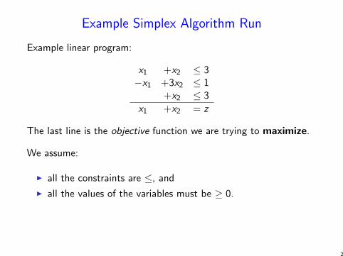
Example Simplex Algorithm Run

Example linear program:

x1 +x2 ≤ 3−x1 +3x2 ≤ 1

+x2 ≤ 3

x1 +x2 = z

The last line is the objective function we are trying to maximize.

We assume:

I all the constraints are ≤, and

I all the values of the variables must be ≥ 0.

2

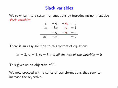
Slack variables

We re-write into a system of equations by introducing non-negativeslack variables:

x1 +x2 +x3 = 3−x1 +3x2 +x4 = 1

+x2 +x5 = 3

x1 +x2 = z

There is an easy solution to this system of equations:

x3 = 3, x4 = 1, x5 = 3 and all the rest of the variables = 0

This gives us an objective of 0.

We now proceed with a series of transformations that seek toincrease the objective.

3

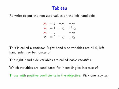
Tableau

Re-write to put the non-zero values on the left-hand side:

x3 = 3 −x1 −x2x4 = 1 +x1 −3x2x5 = 3 −x2z = 0 +x1 +x2

This is called a tableau: Right-hand side variables are all 0, lefthand side may be non-zero.

The right hand side variables are called basic variables.

Which variables are candidates for increasing to increase z?

Those with positive coefficients in the objective. Pick one: say x2.

4

Tableau

Re-write to put the non-zero values on the left-hand side:

x3 = 3 −x1 −x2x4 = 1 +x1 −3x2x5 = 3 −x2z = 0 +x1 +x2

This is called a tableau: Right-hand side variables are all 0, lefthand side may be non-zero.

The right hand side variables are called basic variables.

Which variables are candidates for increasing to increase z?

Those with positive coefficients in the objective. Pick one: say x2.

4

Entering variable

x2 is called the entering variable (we’ll see why in a minute)

How much can we increase x2 by?

So long as none of the basic variables become negative.

We choose the amount to increase based on the strictest equation:

3− x2 ≥ 0 =⇒ x2 ≤ 3 (1)

1− 3x2 ≥ 0 =⇒ x2 ≤ 1/3 (2)

3− x2 ≥ 0 =⇒ x2 ≤ 3 (3)

Constraint (2) is the strictest, so we set x2 = 1/3.

5

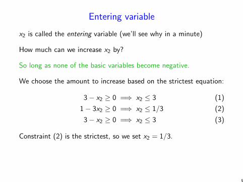
Entering variable

x2 is called the entering variable (we’ll see why in a minute)

How much can we increase x2 by?

So long as none of the basic variables become negative.

We choose the amount to increase based on the strictest equation:

3− x2 ≥ 0 =⇒ x2 ≤ 3 (1)

1− 3x2 ≥ 0 =⇒ x2 ≤ 1/3 (2)

3− x2 ≥ 0 =⇒ x2 ≤ 3 (3)

Constraint (2) is the strictest, so we set x2 = 1/3.

5

The leaving variable

Look at the strictest constraint now:

x4 = 1 + x1 − 3x2 =⇒ x2 = 1/3 + (1/3)x1 − (1/3)x4

If we increase x2 = 1/3, then x4 becomes 0.

We re-write constraint (2) to put x2 on the left-hand side, andsubstitute in for x2 in all the remaining equations:

x3 = 8/3 −(4/3)x1 +(1/3)x4x2 = 1/3 +(1/3)x1 −(1/3)x4x5 = 8/3 −(1/3)x1 +(1/3)x4z = 1/3 +(4/3)x1 −(1/3)x4

This system of equations is equivalent to what we started with, butnow if we set the rhs variables to 0, we get an objective value of1/3. Progress!

6

Pivots

x4 was the leaving variable.

Now which variable can we increase?

x1 is the only variable with a non-negative coefficient in ourobjective. So, we select x1 as the entering variable, and see howmuch we can increase it:

x1 ≤ (8/3)/(4/3) = 2 (4)

x1≥ (1/3)/(−1/3) = −1 (5)

x1 ≤ (8/3)/(1/3) = 8 (6)

Notice only those constraints where x1 has a negative coefficientprovide a constraint!

Constraint (4) is the strictest. So we increase x1 to 2 in the sameway as before.

7

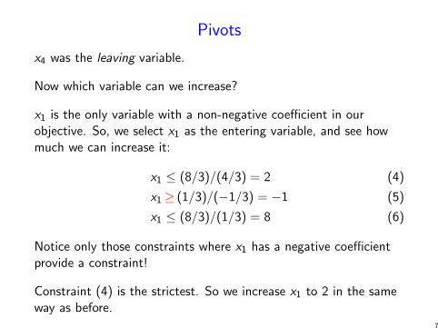
Pivots

x4 was the leaving variable.

Now which variable can we increase?

x1 is the only variable with a non-negative coefficient in ourobjective. So, we select x1 as the entering variable, and see howmuch we can increase it:

x1 ≤ (8/3)/(4/3) = 2 (4)

x1≥ (1/3)/(−1/3) = −1 (5)

x1 ≤ (8/3)/(1/3) = 8 (6)

Notice only those constraints where x1 has a negative coefficientprovide a constraint!

Constraint (4) is the strictest. So we increase x1 to 2 in the sameway as before.

7

Increasing x1 to 2

Look at the strictest constraint:

x3 = 8/3− (4/3)x1 + (1/3)x4 =⇒ x1 = 2− (3/4)x3 − (1/4)x4

Rewrite that constraint in terms of x1, and substitute in for x1everywhere:

x1 = 2 −(3/4)x3 +(1/4)x4x2 = 1 −(1/4)x3 −(1/4)x4x5 = 2 +(1/4)x3 +(1/4)x4z = 3 −x3

Now: all the coefficients in the objective function are ≤ 0, so we’redone. The optimal value is 3 with x1 = 2 and x2 = 1.

Check that these values satisfy the original constraints!

8

Note

I Note that increasing x1 also increased x2. This happenedwhen we substituted in for x1 in the second constraint.

9

Simplex Algorithm In General

1. Write LP with slack variables (slack vars = initial solution)

2. Choose a variable v in the objective with a positive coefficientto increase

3. Among the equations in which v has a negative coefficientqiv , choose the strictest one

This is the one that minimizes −pi/qiv because theequations are all of the form xi = pi + qivxv .

4. Re-write the strictest equation to put v on the left-hand side,and substitute for v everywhere else.

5. If all the coefficients are ≤ 0 in objective, we’re done;otherwise, jump back to step 2.

10

Schematic of a pivot

+-+-+

+

p1p2p3p4p5

z = obj

xi =

xj =

Basic variables

values of basic variables in

current solution

objective value of current solution

candidate entering variable

candidate leaving

variables

11

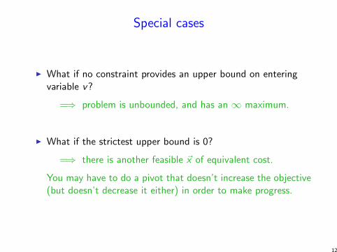
Special cases

I What if no constraint provides an upper bound on enteringvariable v?

=⇒ problem is unbounded, and has an ∞ maximum.

I What if the strictest upper bound is 0?

=⇒ there is another feasible ~x of equivalent cost.

You may have to do a pivot that doesn’t increase the objective(but doesn’t decrease it either) in order to make progress.

12

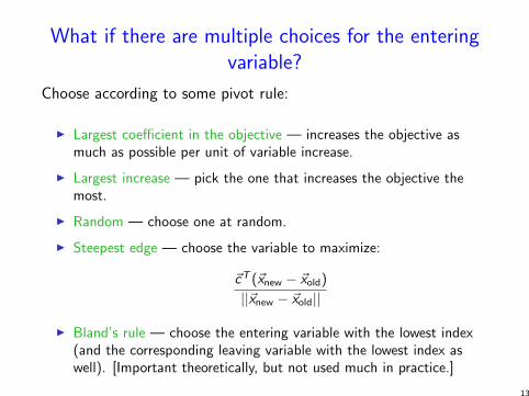
What if there are multiple choices for the enteringvariable?

Choose according to some pivot rule:

I Largest coefficient in the objective — increases the objective asmuch as possible per unit of variable increase.

I Largest increase — pick the one that increases the objective themost.

I Random — choose one at random.

I Steepest edge — choose the variable to maximize:

~cT (~xnew − ~xold)

||~xnew − ~xold||

I Bland’s rule — choose the entering variable with the lowest index(and the corresponding leaving variable with the lowest index aswell). [Important theoretically, but not used much in practice.]

13

How do we know this process will terminate?

In general, this process might not terminate!

If you can always increase the objective function (non-zero upperbound on the entering variable), then it must eventually stop.

It might be that you repeatedly have to choose an entering variablewith a 0 upper bound.

Bland’s rule ensures that you can’t cycle forever.

14

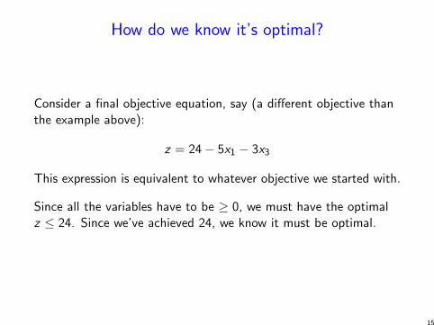
How do we know it’s optimal?

Consider a final objective equation, say (a different objective thanthe example above):

z = 24− 5x1 − 3x3

This expression is equivalent to whatever objective we started with.

Since all the variables have to be ≥ 0, we must have the optimalz ≤ 24. Since we’ve achieved 24, we know it must be optimal.

15

Initialization

We made one implicit assumption in the discussion above: thatinitially setting the non-slack variables to 0 would give us a feasiblesolution.

This is not the case if the bi values are < 0:

x3 = 3 −x1 −x2x4 = −1 +x1 −3x2x5 = 3 −x2z = 0 +x1 +x2

Here, we’d get a “solution” with x4 < 0, which is not allowed.

We solve an auxiliary LP problem to find the initial solution.

16

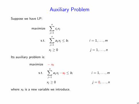
Auxiliary Problem

Suppose we have LP:

maximizen∑

j=1

cjxj

s.t.n∑

j=1

aijxj ≤ bi i = 1, . . . ,m

xj ≥ 0 j = 1, . . . , n

Its auxiliary problem is:

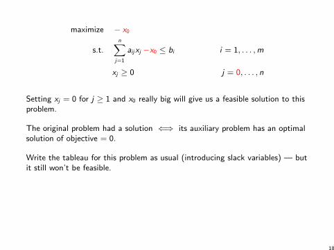
maximize − x0

s.t.n∑

j=1

aijxj −x0 ≤ bi i = 1, . . . ,m

xj ≥ 0 j = 0, . . . , n

where x0 is a new variable we introduce.

17

maximize − x0

s.t.n∑

j=1

aijxj −x0 ≤ bi i = 1, . . . ,m

xj ≥ 0 j = 0, . . . , n

Setting xj = 0 for j ≥ 1 and x0 really big will give us a feasible solution to thisproblem.

The original problem had a solution ⇐⇒ its auxiliary problem has an optimalsolution of objective = 0.

Write the tableau for this problem as usual (introducing slack variables) — butit still won’t be feasible.

18

Auxiliary Tableau

-x0z =

w1 =

w2 =

w3 =

w4 =

w5 =

+1x0+1x0+1x0+1x0+1x0

All +1 coeff. b/c original equations

all had -1x0

+A-B

+C-D+E

The original b vector (which includes some

negative entries)

The

slac

k va

riabl

es

Suppose −B is the most negative entry. Rewrite that equation in terms of x0:

x0 = +B + terms involving variables

Now substitute the red part in for x0 in every other equation.

This will add B to every constant term =⇒ all the constant terms becomepositive (since −B was the most negative).

19

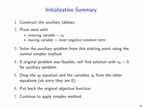
Initialization Summary

1. Construct the auxiliary tableau.

2. Pivot once withI entering variable = x0I leaving variable = most negative constant term

3. Solve the auxiliary problem from this starting point using thenormal simplex method.

4. If original problem was feasible, will find solution with x0 = 0for auxiliary problem.

5. Drop the x0 equation and the variables x0 from the otherequations (ok since they are 0).

6. Put back the original objective function.

7. Continue to apply simplex method.

20

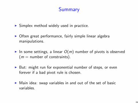
Summary

I Simplex method widely used in practice.

I Often great performance, fairly simple linear algebramanipulations.

I In some settings, a linear O(m) number of pivots is observed(m = number of constraints).

I But: might run for exponential number of steps, or evenforever if a bad pivot rule is chosen.

I Main idea: swap variables in and out of the set of basicvariables.

21