CS675: Convex and Combinatorial Optimization Fall 2016 The...
41
CS675: Convex and Combinatorial Optimization Fall 2016 The Simplex Algorithm Instructor: Shaddin Dughmi
Transcript of CS675: Convex and Combinatorial Optimization Fall 2016 The...
CS675: Convex and Combinatorial OptimizationFall 2016
The Simplex Algorithm
Instructor: Shaddin Dughmi
Algorithms for Convex Optimization
We will look at 2 algorithms in detail: Simplex and Ellipsoid.If there is time, we might also look at interior point methods (e.g.gradient descent and variants). These are important in practice.

History and Basics of the Simplex Algorithm
First methodical procedure for solving linear programsDeveloped by George Dantzig in 1947Considered one of the most influential algorithms of the 20thcentury
Really a family of algorithms, parametrized by a “pivot rule”Efficient in practice, leading to conjectures that it runs inpolynomial timeIn 1972, Klee and Minty exhibited worst-case examples that takeexponential time, at least for some of the most popular simplexpivot rulesThis spurred development of the Ellipsoid method, interior pointmethods, . . .
History and Basics of the Simplex Algorithm
First methodical procedure for solving linear programsDeveloped by George Dantzig in 1947Considered one of the most influential algorithms of the 20thcenturyReally a family of algorithms, parametrized by a “pivot rule”
Efficient in practice, leading to conjectures that it runs inpolynomial timeIn 1972, Klee and Minty exhibited worst-case examples that takeexponential time, at least for some of the most popular simplexpivot rulesThis spurred development of the Ellipsoid method, interior pointmethods, . . .
History and Basics of the Simplex Algorithm
First methodical procedure for solving linear programsDeveloped by George Dantzig in 1947Considered one of the most influential algorithms of the 20thcenturyReally a family of algorithms, parametrized by a “pivot rule”Efficient in practice, leading to conjectures that it runs inpolynomial timeIn 1972, Klee and Minty exhibited worst-case examples that takeexponential time, at least for some of the most popular simplexpivot rules
This spurred development of the Ellipsoid method, interior pointmethods, . . .
History and Basics of the Simplex Algorithm
First methodical procedure for solving linear programsDeveloped by George Dantzig in 1947Considered one of the most influential algorithms of the 20thcenturyReally a family of algorithms, parametrized by a “pivot rule”Efficient in practice, leading to conjectures that it runs inpolynomial timeIn 1972, Klee and Minty exhibited worst-case examples that takeexponential time, at least for some of the most popular simplexpivot rulesThis spurred development of the Ellipsoid method, interior pointmethods, . . .

Outline
1 Description of The Simplex Algorithm
2 Properties
3 Initialization

Linear Programming
We consider a standard form LP written as follows for convenience
maximize cᵀxsubject to Ax � b
minimize yᵀbsubject to yᵀA = cᵀ
y � 0
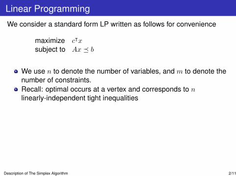
We use n to denote the number of variables, and m to denote thenumber of constraints.
Recall: optimal occurs at a vertex and corresponds to nlinearly-independent tight inequalitiesWe assume we are given a starting vertex x0 as input, and want tocompute optimal vertex x∗
This is Phase IIPhase I, finding an initial vertex, involves solving another LP. Wewill come back to this at the end.
Degeneracy: a vertex with > n tight inequalitiesWe will mostly assume this away to save ourselves a headache
Incidentally, algorithm will produce optimal dual y∗ as well.
Description of The Simplex Algorithm 2/11
Linear Programming
We consider a standard form LP written as follows for convenience
maximize cᵀxsubject to Ax � b
minimize yᵀbsubject to yᵀA = cᵀ
y � 0
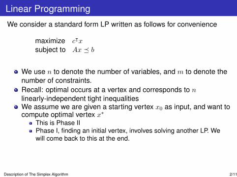
We use n to denote the number of variables, and m to denote thenumber of constraints.Recall: optimal occurs at a vertex and corresponds to nlinearly-independent tight inequalities
We assume we are given a starting vertex x0 as input, and want tocompute optimal vertex x∗
This is Phase IIPhase I, finding an initial vertex, involves solving another LP. Wewill come back to this at the end.
Degeneracy: a vertex with > n tight inequalitiesWe will mostly assume this away to save ourselves a headache
Incidentally, algorithm will produce optimal dual y∗ as well.
Description of The Simplex Algorithm 2/11
Linear Programming
We consider a standard form LP written as follows for convenience
maximize cᵀxsubject to Ax � b
minimize yᵀbsubject to yᵀA = cᵀ
y � 0
We use n to denote the number of variables, and m to denote thenumber of constraints.Recall: optimal occurs at a vertex and corresponds to nlinearly-independent tight inequalitiesWe assume we are given a starting vertex x0 as input, and want tocompute optimal vertex x∗
This is Phase IIPhase I, finding an initial vertex, involves solving another LP. Wewill come back to this at the end.
Degeneracy: a vertex with > n tight inequalitiesWe will mostly assume this away to save ourselves a headache
Incidentally, algorithm will produce optimal dual y∗ as well.
Description of The Simplex Algorithm 2/11

Linear Programming
We consider a standard form LP written as follows for convenience
maximize cᵀxsubject to Ax � b
minimize yᵀbsubject to yᵀA = cᵀ
y � 0
We use n to denote the number of variables, and m to denote thenumber of constraints.Recall: optimal occurs at a vertex and corresponds to nlinearly-independent tight inequalitiesWe assume we are given a starting vertex x0 as input, and want tocompute optimal vertex x∗
This is Phase IIPhase I, finding an initial vertex, involves solving another LP. Wewill come back to this at the end.
Degeneracy: a vertex with > n tight inequalitiesWe will mostly assume this away to save ourselves a headache
Incidentally, algorithm will produce optimal dual y∗ as well.Description of The Simplex Algorithm 2/11
Recall: Physical Interpretation of LP
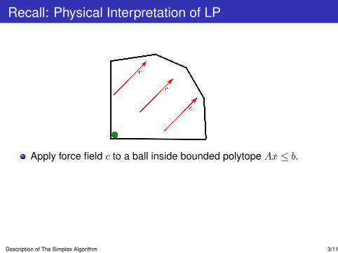
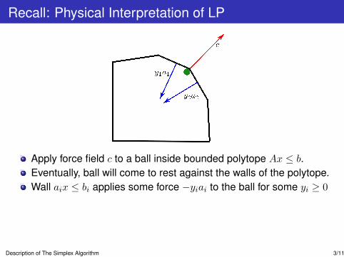
Apply force field c to a ball inside bounded polytope Ax ≤ b.
Eventually, ball will come to rest against the walls of the polytope.Wall aix ≤ bi applies some force −yiai to the ball for some yi ≥ 0
Since the ball is still, cT =∑
i yiai = yTA.At optimality, only the walls adjacent to the ball push(Complementary Slackness)
Necessary and sufficient for optimality, given dual-feasible y
Description of The Simplex Algorithm 3/11
Recall: Physical Interpretation of LP
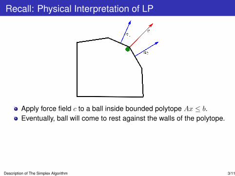
Apply force field c to a ball inside bounded polytope Ax ≤ b.Eventually, ball will come to rest against the walls of the polytope.
Wall aix ≤ bi applies some force −yiai to the ball for some yi ≥ 0
Since the ball is still, cT =∑
i yiai = yTA.At optimality, only the walls adjacent to the ball push(Complementary Slackness)
Necessary and sufficient for optimality, given dual-feasible y
Description of The Simplex Algorithm 3/11
Recall: Physical Interpretation of LP
Apply force field c to a ball inside bounded polytope Ax ≤ b.Eventually, ball will come to rest against the walls of the polytope.Wall aix ≤ bi applies some force −yiai to the ball for some yi ≥ 0
Since the ball is still, cT =∑
i yiai = yTA.At optimality, only the walls adjacent to the ball push(Complementary Slackness)
Necessary and sufficient for optimality, given dual-feasible y
Description of The Simplex Algorithm 3/11

Recall: Physical Interpretation of LP
Apply force field c to a ball inside bounded polytope Ax ≤ b.Eventually, ball will come to rest against the walls of the polytope.Wall aix ≤ bi applies some force −yiai to the ball for some yi ≥ 0
Since the ball is still, cT =∑
i yiai = yTA.
At optimality, only the walls adjacent to the ball push(Complementary Slackness)
Necessary and sufficient for optimality, given dual-feasible y
Description of The Simplex Algorithm 3/11

Recall: Physical Interpretation of LP
Apply force field c to a ball inside bounded polytope Ax ≤ b.Eventually, ball will come to rest against the walls of the polytope.Wall aix ≤ bi applies some force −yiai to the ball for some yi ≥ 0
Since the ball is still, cT =∑
i yiai = yTA.At optimality, only the walls adjacent to the ball push(Complementary Slackness)
Necessary and sufficient for optimality, given dual-feasible yDescription of The Simplex Algorithm 3/11

Informal Description
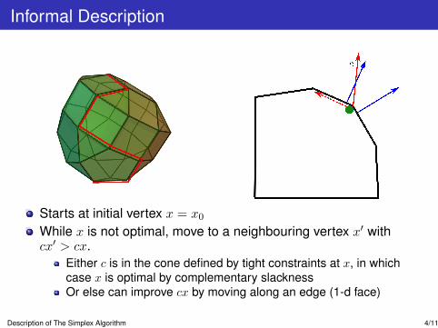
Starts at initial vertex x = x0While x is not optimal, move to a neighbouring vertex x′ withcx′ > cx.
Either c is in the cone defined by tight constraints at x, in whichcase x is optimal by complementary slacknessOr else can improve cx by moving along an edge (1-d face)
Description of The Simplex Algorithm 4/11
Informal Description
Starts at initial vertex x = x0While x is not optimal, move to a neighbouring vertex x′ withcx′ > cx.
Either c is in the cone defined by tight constraints at x, in whichcase x is optimal by complementary slacknessOr else can improve cx by moving along an edge (1-d face)
Description of The Simplex Algorithm 4/11
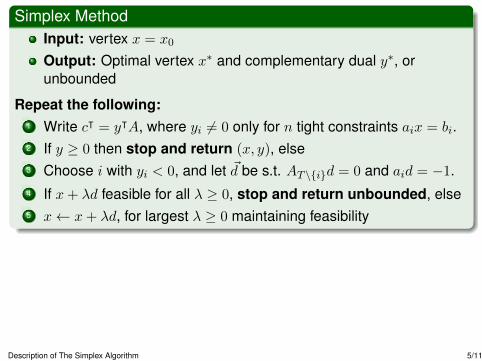
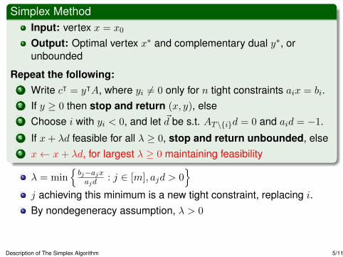
Simplex MethodInput: vertex x = x0
Output: Optimal vertex x∗ and complementary dual y∗, orunbounded
Repeat the following:1 Write cᵀ = yᵀA, where yi 6= 0 only for n tight constraints aix = bi.2 If y ≥ 0 then stop and return (x, y), else3 Choose i with yi < 0, and let ~d be s.t. AT\{i}d = 0 and aid = −1.4 If x+ λd feasible for all λ ≥ 0, stop and return unbounded, else5 x← x+ λd, for largest λ ≥ 0 maintaining feasibility
Description of The Simplex Algorithm 5/11

Simplex MethodInput: vertex x = x0
Output: Optimal vertex x∗ and complementary dual y∗, orunbounded
Repeat the following:1 Write cᵀ = yᵀA, where yi 6= 0 only for n tight constraints aix = bi.2 If y ≥ 0 then stop and return (x, y), else3 Choose i with yi < 0, and let ~d be s.t. AT\{i}d = 0 and aid = −1.4 If x+ λd feasible for all λ ≥ 0, stop and return unbounded, else5 x← x+ λd, for largest λ ≥ 0 maintaining feasibility
Let T be set of tight rows. yᵀTAT = cᵀ
Gaussian elimination
Description of The Simplex Algorithm 5/11

Simplex MethodInput: vertex x = x0
Output: Optimal vertex x∗ and complementary dual y∗, orunbounded
Repeat the following:1 Write cᵀ = yᵀA, where yi 6= 0 only for n tight constraints aix = bi.2 If y ≥ 0 then stop and return (x, y), else3 Choose i with yi < 0, and let ~d be s.t. AT\{i}d = 0 and aid = −1.4 If x+ λd feasible for all λ ≥ 0, stop and return unbounded, else5 x← x+ λd, for largest λ ≥ 0 maintaining feasibility
y is a dual satisfying complementary slackness with xTherefore both are optimal
Description of The Simplex Algorithm 5/11
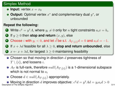
Simplex MethodInput: vertex x = x0
Output: Optimal vertex x∗ and complementary dual y∗, orunbounded
Repeat the following:1 Write cᵀ = yᵀA, where yi 6= 0 only for n tight constraints aix = bi.2 If y ≥ 0 then stop and return (x, y), else3 Choose i with yi < 0, and let ~d be s.t. AT\{i}d = 0 and aid = −1.4 If x+ λd feasible for all λ ≥ 0, stop and return unbounded, else5 x← x+ λd, for largest λ ≥ 0 maintaining feasibility
Chosen so that moving in direction d preserves tightness ofT \ {i}, and loosens i.AT is full-rank, therefore null(AT\{i}) is a 1-dimensional subspacewhich is not normal to aiChoose d ∈ null(AT\{i}) appropriately.Moving in direction d improves objective: cᵀd = yᵀAd = yiaid > 0
Description of The Simplex Algorithm 5/11

Simplex MethodInput: vertex x = x0
Output: Optimal vertex x∗ and complementary dual y∗, orunbounded
Repeat the following:1 Write cᵀ = yᵀA, where yi 6= 0 only for n tight constraints aix = bi.2 If y ≥ 0 then stop and return (x, y), else3 Choose i with yi < 0, and let ~d be s.t. AT\{i}d = 0 and aid = −1.4 If x+ λd feasible for all λ ≥ 0, stop and return unbounded, else5 x← x+ λd, for largest λ ≥ 0 maintaining feasibility
i.e. Ad ≤ 0
Description of The Simplex Algorithm 5/11
Simplex MethodInput: vertex x = x0
Output: Optimal vertex x∗ and complementary dual y∗, orunbounded
Repeat the following:1 Write cᵀ = yᵀA, where yi 6= 0 only for n tight constraints aix = bi.2 If y ≥ 0 then stop and return (x, y), else3 Choose i with yi < 0, and let ~d be s.t. AT\{i}d = 0 and aid = −1.4 If x+ λd feasible for all λ ≥ 0, stop and return unbounded, else5 x← x+ λd, for largest λ ≥ 0 maintaining feasibility
λ = min{bj−ajxajd
: j ∈ [m], ajd > 0}
j achieving this minimum is a new tight constraint, replacing i.By nondegeneracy assumption, λ > 0
Description of The Simplex Algorithm 5/11

Outline
1 Description of The Simplex Algorithm
2 Properties
3 Initialization
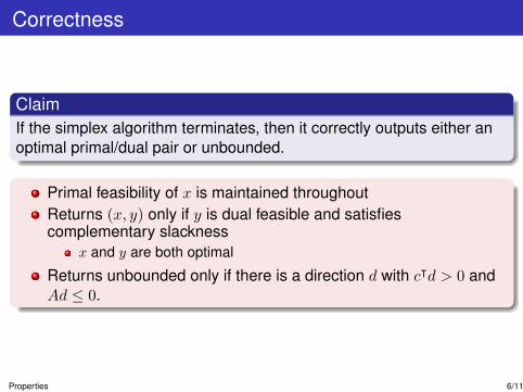
Correctness
ClaimIf the simplex algorithm terminates, then it correctly outputs either anoptimal primal/dual pair or unbounded.
Primal feasibility of x is maintained throughoutReturns (x, y) only if y is dual feasible and satisfiescomplementary slackness
x and y are both optimal
Returns unbounded only if there is a direction d with cᵀd > 0 andAd ≤ 0.
Properties 6/11
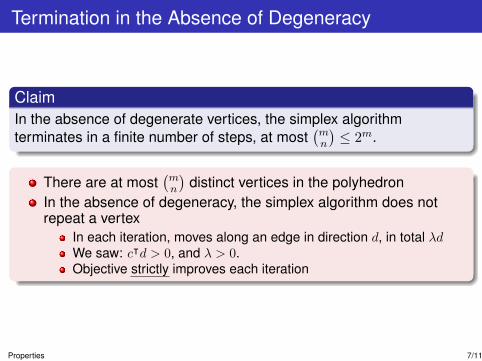
Termination in the Absence of Degeneracy
ClaimIn the absence of degenerate vertices, the simplex algorithmterminates in a finite number of steps, at most
(mn
)≤ 2m.
There are at most(mn
)distinct vertices in the polyhedron
In the absence of degeneracy, the simplex algorithm does notrepeat a vertex
In each iteration, moves along an edge in direction d, in total λdWe saw: cᵀd > 0, and λ > 0.Objective strictly improves each iteration
Properties 7/11
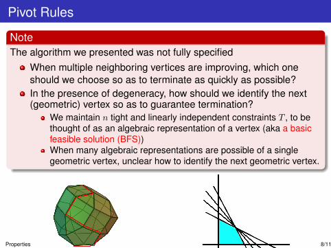
Pivot Rules
NoteThe algorithm we presented was not fully specified
When multiple neighboring vertices are improving, which oneshould we choose so as to terminate as quickly as possible?In the presence of degeneracy, how should we identify the next(geometric) vertex so as to guarantee termination?
We maintain n tight and linearly independent constraints T , to bethought of as an algebraic representation of a vertex (aka a basicfeasible solution (BFS))When many algebraic representations are possible of a singlegeometric vertex, unclear how to identify the next geometric vertex.
Properties 8/11

Pivot Rules
Both concerns are addressed by the use of a pivot rule, whichdetermines the order in which we examine algebraic vertices.
Pivot ruleA rule for selecting which i leaves T , and which j enters T , whenmultiple choices are possible either because of multiple improvingneighbors or degeneracy. Examples:
Bland’s rule: Choose lowest indexed i, then lowest indexed jLexicographic: Maintain an order over rows, and move from T tothe lexicographically smallest possible T ′.Perturbation: perturb entries of b by a small value to removedegeneracy. This perturbation can be purely symbolic.
Properties 8/11

Runtime and Termination
Many pivot rules, like the ones we mentioned, have been shown tonever cycle over algebraic vertices
Guarantees termination in general, even in the presence ofdegeneraciesSee book and notes for proofs.
However, no pivot rules have been shown to guarantee apolynomial number of pivots
Even if no degeneracies.
In 1972, Klee and Minty exhibited a family of examples that lead toexponential worst-case runtime for some widely-used pivot rules
Properties 9/11
Runtime and Termination
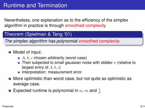
Nevertheless, one explanation as to the efficiency of the simplexalgorithm in practice is through smoothed complexity
Theorem (Spielman & Teng ’01)The simplex algorithm has polynomial smoothed complexity.
Model of input:A, b, c chosen arbitrarily (worst case)Then subjected to small gaussian noise with stddev σ (relative tolargest entry of A, b, c)Interpretation: measurement error
More optimistic than worst case, but not quite as optimistic asaverage case.Expected runtime is polynomial in n, m and 1
σ
Properties 9/11

Runtime and Termination
Open QuestionIs there a pivot rule which guarantees a polynomial number of pivots ofthe simplex algorithm in the worst case?
Why is this important?Would yield a strongly polynomial algorithm for LPIf true, resolves in the affirmative a classic open question inpolyhedral combinatorics
Polynomial Hirsch Conjecture: Is the diameter of the edge-vertexgraph of an m-facet polytope in n-dimensional space bounded by apolynomial in n and m?
Properties 9/11
Outline
1 Description of The Simplex Algorithm
2 Properties
3 Initialization

Initialization
Solving a Linear Program via the Simplex MethodPhase I: Find a vertex x0.Phase II: Run the simplex algorithm starting from x0
So far, we have looked only at phase IIFor phase I, we pose a different LP whose optimal solution is avertex, if one exists
Initialization 10/11
Phase I
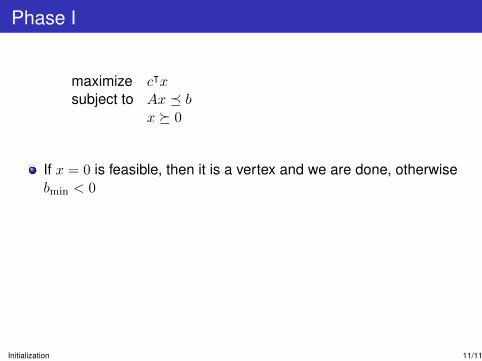
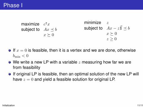
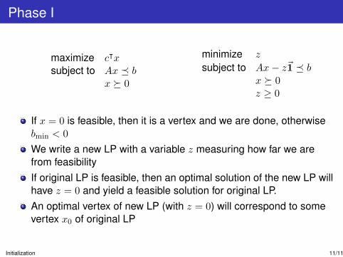
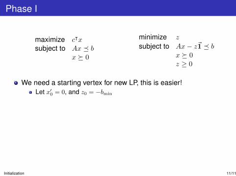
maximize cᵀxsubject to Ax � b
x � 0
minimize z
subject to Ax− z~1 � bx � 0z ≥ 0
If x = 0 is feasible, then it is a vertex and we are done, otherwisebmin < 0
We write a new LP with a variable z measuring how far we arefrom feasibilityIf original LP is feasible, then an optimal solution of the new LP willhave z = 0 and yield a feasible solution for original LP.An optimal vertex of new LP (with z = 0) will correspond to somevertex x0 of original LPWe need a starting vertex for new LP, this is easier!
Let x′0 = 0, and z0 = −bmin
Running simplex on new LP with starting vertex (x′0, z0), we getstarting vertex x0 for original LP.
Initialization 11/11

Phase I
maximize cᵀxsubject to Ax � b
x � 0
minimize z
subject to Ax− z~1 � bx � 0z ≥ 0
If x = 0 is feasible, then it is a vertex and we are done, otherwisebmin < 0
We write a new LP with a variable z measuring how far we arefrom feasibility
If original LP is feasible, then an optimal solution of the new LP willhave z = 0 and yield a feasible solution for original LP.An optimal vertex of new LP (with z = 0) will correspond to somevertex x0 of original LPWe need a starting vertex for new LP, this is easier!
Let x′0 = 0, and z0 = −bmin
Running simplex on new LP with starting vertex (x′0, z0), we getstarting vertex x0 for original LP.
Initialization 11/11
Phase I
maximize cᵀxsubject to Ax � b
x � 0
minimize z
subject to Ax− z~1 � bx � 0z ≥ 0
If x = 0 is feasible, then it is a vertex and we are done, otherwisebmin < 0
We write a new LP with a variable z measuring how far we arefrom feasibilityIf original LP is feasible, then an optimal solution of the new LP willhave z = 0 and yield a feasible solution for original LP.
An optimal vertex of new LP (with z = 0) will correspond to somevertex x0 of original LPWe need a starting vertex for new LP, this is easier!
Let x′0 = 0, and z0 = −bmin
Running simplex on new LP with starting vertex (x′0, z0), we getstarting vertex x0 for original LP.
Initialization 11/11
Phase I
maximize cᵀxsubject to Ax � b
x � 0
minimize z
subject to Ax− z~1 � bx � 0z ≥ 0
If x = 0 is feasible, then it is a vertex and we are done, otherwisebmin < 0
We write a new LP with a variable z measuring how far we arefrom feasibilityIf original LP is feasible, then an optimal solution of the new LP willhave z = 0 and yield a feasible solution for original LP.An optimal vertex of new LP (with z = 0) will correspond to somevertex x0 of original LP
We need a starting vertex for new LP, this is easier!Let x′0 = 0, and z0 = −bmin
Running simplex on new LP with starting vertex (x′0, z0), we getstarting vertex x0 for original LP.
Initialization 11/11
Phase I
maximize cᵀxsubject to Ax � b
x � 0
minimize z
subject to Ax− z~1 � bx � 0z ≥ 0
We need a starting vertex for new LP, this is easier!Let x′0 = 0, and z0 = −bmin
Running simplex on new LP with starting vertex (x′0, z0), we getstarting vertex x0 for original LP.
Initialization 11/11

Phase I
maximize cᵀxsubject to Ax � b
x � 0
minimize z
subject to Ax− z~1 � bx � 0z ≥ 0
We need a starting vertex for new LP, this is easier!Let x′0 = 0, and z0 = −bmin
Running simplex on new LP with starting vertex (x′0, z0), we getstarting vertex x0 for original LP.
Initialization 11/11