The Schr odinger Equation - University of Illinois at Urbana ... 3 The Schr odinger Equation 3.1...

Chapter 3

The Schrodinger Equation

3.1 Derivation of the Schrodinger Equation

We will consider now the propagation of a wave function ψ(~r, t) by an infinitesimal time step ε. Itholds then according to (2.5)

ψ(~r, t+ ε) =∫

Ωd3r0 φ(~r, t+ ε|~r0, t)ψ(~r0, t) . (3.1)

We will expand the l.h.s. and the r.h.s. of this equation in terms of powers of ε and we willdemonstrate that the terms of order ε require that ψ(~r, t) satisfies a partial differential equation,namely the Schrodinger equation. For many situations, but by no means all, the Schrodingerequation provides the simpler avenue towards describing quantum systems than the path ingralformulation of Section 2. Notable exceptions are non-stationary systems involving time-dependentlinear and quadratic Lagrangians.The propagator in (3.1) can be expressed through the discretization scheme (2.20, 2.21). In thelimit of very small ε it is sufficient to employ a single discretization interval in (2.20) to evaluatethe propagator. Generalizing (2.20) to R3 one obtains then for small ε

φ(~r, t+ ε|~r0, t) =[ m

2πi~ε

] 32 exp

i

~

[m

2(~r − ~r0)2

ε− ε U(~r, t)

]. (3.2)

From this follows

ψ(~r, t+ ε) =∫

Ωd3r0

[ m

2πi~ε

] 32 exp

i

~

[m

2(~r − ~r0)2

ε− ε U(~r, t)

]ψ(~r0, t) . (3.3)

In order to carry out the integration we set ~r0 = ~r + ~s and use ~s as the new integration variable.We will denote the components of ~s by (x1, x2, x3)T . This yields

ψ(~r, t+ ε) =∫ +∞−∞ dx1

∫ +∞−∞ dx2

∫ +∞−∞ dx3

[m

2πi~ε

] 32 ×

× exp(i

~

m

2x2

1 + x22 + x2

3

ε− ε U(~r, t)

)︸︷︷︸

even in x1, x2, , x3

ψ(~r + ~s, t) . (3.4)

51

52 Schrodinger Equation

It is important to note that the integration is not over ~r, but over ~s = (x1, x2, x3)T , e.g. U(~r, t) is aconstant with respect to this integration. The integration involves only the wave function ψ(~r+~s, t)and the kinetic energy term. Since the latter contributes to (3.4) only for small x2

1 +x22 +x2

3 valueswe expand

ψ(~r + ~s, t) = ψ(~r, t) +3∑j=1

xj∂

∂xjψ(~r, t) +

12

3∑j,k=1

xjxk∂2

∂xj∂xkψ(~r, t) + . . . (3.5)

assuming that only the leading terms contribute, a supposition which will be examined below. Sincethe kinetic energy contribution in (3.4) is even in all three coordinates x1, x2, x3, only terms of theexpansion (3.5) which are even separately in all three coordinates yield non-vanishing contributions.It is then sufficient to consider the terms

ψ(~r, t) ; 12

∑3j=1 x

2j∂2

∂x2jψ(~r, t) ; 1

4

∑3j,k=1 x

2jx

2k

∂4

∂x2j∂x

2kψ(~r, t) ;

112

∑3j=1 x

4j∂4

∂x4jψ(~r, t) ; . . . (3.6)

of the expansion of ψ(~r + ~s, t).Obviously, we need then to evaluate integrals of the type

In(a) =∫ +∞

−∞dx x2n exp

(i a x2

), n = 0, 1, 2 (3.7)

According to (2.36) holds

I0(a) =

√iπ

a(3.8)

Inspection of (3.7) shows

In+1(a) =1i

∂

∂aIn(a). (3.9)

Starting from (3.8) one can evaluate recursively all integrals In(a). It holds

I1(a) =i

2a

√iπ

a; I2(a) = − 3

4a2

√iπ

a, . . . (3.10)

It is now important to note that in case of integral (3.4) one identifies

1a

=2 ε ~m

= O(ε) (3.11)

and, consequently, the terms collected in (3.6) make contributions of the order

O(ε32 ) , O(ε

52 ) , O(ε

72 ) , O(ε

72 ) . (3.12)

Here one needs to note that we are actually dealing with a three-fold integral. According to (3.11)holds [ m

2πi~ε

] 32 ×

[i π

a

] 32

= 1 (3.13)

3.2: Boundary Conditions 53

and one can conclude, using (3.10),

ψ(~r, t+ ε) = exp[− iε~

U(~r, t)] [

ψ(~r, t) +14

2iε~m∇2ψ(~r, t) + O(ε2)

]. (3.14)

This expansion in terms of powers of ε suggests that we also expand

ψ(~r, t+ ε) = ψ(~r, t) + ε∂

∂tψ(~r, t) + O(ε2) (3.15)

and

exp[− iε~

U(~r, t)]

= 1 − iε

~

U(~r, t) + O(ε2) . (3.16)

Inserting this into (3.14) results in

ψ(~r, t) + ε ∂∂tψ(~r, t) = ψ(~r, t) − iε

~

U(~r, t)ψ(~r, t)

+iε

~

~2

2m∇2ψ(~r, t) + O(ε2) . (3.17)

Obviously, this equation is trivially satisfied to order O(ε0). In order O(ε) the equation reads

i~∂

∂tψ(~r, t) =

[− ~

2

2m∇2 + U(~r, t)

]ψ(~r, t) . (3.18)

This is the celebrated time-dependent Schrodinger equation. This equation is often written in theform

i~∂

∂tψ(~r, t) = H ψ(~r, t) (3.19)

where

H = − ~2

2m∇2 + U(~r, t) . (3.20)

3.2 Boundary Conditions

The time-dependent Schrodinger equation is a partial differential equation, 1st order in time, 2ndorder in the spatial variables and linear in the solution ψ(~r, t). The following general remarks canbe made about the solution.Due to its linear character any linear combination of solutions of the time-dependent Schrodingerequation is also a solution.The 1st order time derivative requires that for any solution a single temporal condition needs to bespecified, e.g., ψ(~r, t1) = f(~r). Usually, one specifies the so-called initial condition, i.e., a solutionis thought for t ≥ t0 and the solution is specified at the intial time t0.The 2nd order spatial derivatives require that one specifies also properties of the solution on aclosed boundary ∂Ω surrounding the volume Ω in which a solution is to be determined. We willderive briefly the type of boundary conditions encountered. As we will discuss in Chapter 5 belowthe solutions of the Schrodinger equation are restricted to particular Hilbert spaces H which are


linear vector spaces of functions f(~r) in which a scalar product between two elements f, g ∈ H isdefined as follows

〈f |g〉Ω =∫

Ωd3rf∗(~r)g(~r) (3.21)

This leads one to consider the integral

〈f |H |g〉Ω =∫

Ωd3rf∗(~r) H g(~r) (3.22)

where H is defined in (3.20). Interchanging f∗(~r) and g(~r) results in

〈g|H |f〉Ω =∫

Ωd3r g(~r) Hf∗(~r) . (3.23)

Since H is a differential operator the expressions (3.22) and (3.23), in principle, differ from eachother. The difference between the integrals is

〈g|H |f〉Ω = − 〈g|H |f〉Ω

=∫

Ωd3rf∗(~r)

(− ~

2

2m∇2

)g(~r) −

∫Ωd3rg(~r)

(− ~

2

2m∇2

)f∗(~r)

+∫

Ωd3rf∗(~r)U(~r, t) g(~r) −

∫Ωd3rg(~r)U(~r, t), f∗(~r)

= − ~2

2m

∫Ωd3rf∗(~r)

(∇2

)g(~r) −

∫Ωd3rg(~r)

(∇2

)f∗(~r) (3.24)

Using Green’s theorem1 ∫Ω d

3r(f∗(~r)∇2 g(~r) − g(~r)∇2 f∗(~r)

)=∫∂Ω d~a · ( f∗(~r)∇g(~r) − g(~r)∇f∗(~r) ) (3.25)

one obtains the identity

〈f | H |g〉Ω = 〈g| H |f〉Ω +∫∂Ωd~a · ~P (f∗, g|~r) (3.26)

where∫∂Ω d~a · ~A(~r) denotes an integral over the surface ∂Ω of the volume Ω, the surface elements

d~a pointing out of the surface in a direction normal to the surface and the vector–valued function~A(~r) is taken at points ~r ∈ ∂Ω. In (3.26) the vector–valued function ~P (f∗, g|~r) is called theconcomitant of H and is

~P (f∗, g|~r) = − ~2

2m( f∗(~r)∇g(~r) − g(~r)∇f∗(~r) ) (3.27)

We will postulate below that H is an operator in H which represents energy. Since energy is a realquantity one needs to require that the eigenvalues of the operator H are real and, hence, that H ishermitian2. The hermitian property, however, implies

〈f | H |g〉Ω = 〈g| H |f〉Ω (3.28)1See, for example, Calssical Electrodynamics, 2nd Ed., J. D. Jackson, (John Wiley, New York, 1975), Chapter 1.2The reader is advised to consult a reference text on ‘Linear Algebra’ to follow this argument.

3.3: Particle Flux 55

and, therefore, we can only allow functions which make the differential d~a · ~P (f∗, g|~r) vanish on∂Ω. It must hold then for all f ∈ H

f(~r) = 0 ∀~r, ~r ∈ ∂Ω (3.29)

ord~a · ∇f(~r) = 0 ∀~r, ~r ∈ ∂Ω (3.30)

Note that these boundary conditions are linear in f , i.e., if f and g satisfy these conditions thanalso does any linear combination αf + βg. Often the closed surface of a volume ∂Ω is the unionof disconnected surfaces3 ∂Ωj , i.e., ∂Ω = ∂Ω1 ∩ ∂Ω2 ∩ ∂Ω3 ∩ . . . In this case one can postulateboth conditions (3.29, 3.30) each condition holding on an entire surface ∂Ωj . However, to avoiddiscontinuities in ψ(~r, t) on a single connected surface ∂Ωj only either one of the conditions (3.29,3.30) can be postulated.A most common boundary condition is encountered for the volume Ω = ~R3 in which case onepostulates

lim|~r|→∞

f(~r) = 0 “natural boundary condition” . (3.31)

In fact, in this case also all derivatives of f(~r) vanish at infinity. The latter property stems fromthe fact that the boundary condition (3.31) usually arises when a particle existing in a bound stateis described. In this case one can expect that the particle density is localized in the area where theenergy of the particle exceeds the potential eenrgy, and that the density decays rapidly when onemoves away from that area. Since the total probability of finding the particle anywhere in space is∫

d3r|f(~r)|2 = 1 (3.32)

the wave function must decay for |~r| → ∞ rapidly enough to be square integrable, i.e., obey (3.32),e.g., like exp(−κr), κ > 0 or like r−α, α > 2. In either case does f(~r) and all of its derivativesvanish asymptotically.

3.3 Particle Flux and Schrodinger Equation

The solution of the Schrodinger equation is the wave function ψ(~r, t) which describes the state ofa particle moving in the potential U(~r, t). The observable directly linked to the wave function isthe probability to find the particle at position ~r at time t, namely, |ψ(~r, t)|2. The probability toobserve the particle anywhere in the subvolume ω ⊂ Ω is

p(ω, t) =∫ωd3r |ψ(~r, t)|2 . (3.33)

The time derivative of p(ω, t) is

∂tp(ω, t) =∫ωd3r [ψ∗(~r, t)∂tψ(~r, t) + ψ(~r, t)∂tψ∗(~r, t) ] . (3.34)

3An example is a volume between two concentric spheres, in which case ∂Ω1 is the inner sphere and ∂Ω2 is theouter sphere.


Using (3.19) and its conjugate complex4

− i~ ∂∂tψ∗(~r, t) = H ψ∗(~r, t) (3.35)

yields

i~∂tp(ω, t) =∫ωd3r

[ψ∗(~r, t) H ψ(~r, t) − ψ(~r, t) H ψ∗(~r, t)

]. (3.36)

According to (3.26, 3.27) this can be written

i~∂tp(ω, t) =∫∂ωd~a · ~P (ψ∗(~r, t), ψ(~r, t)~r, t) . (3.37)

If one applies this identity to ω = Ω one obtains according to (3.29, 3.30) ∂tp(Ω, t) = 0. Accord-ingly the probability to observe the particle anywhere in the total volume Ω is constant. A naturalchoice for this constant is 1. One can multiply the solution of (3.18) by any complex number andaccordingly one can define ψ(~r, t) such that∫

Ωd3r|ψ(~r, t)|2 = 1 (3.38)

holds. One refers to such solution as normalized. We will assume in the remainder of this Sectionthat the solutions discussed are normalized. Note that for a normalized wave function the quantity

ρ(~r, t) = |ψ(~r, t)|2 (3.39)

is a probability density with units 1/volume.The surface integral (3.37) can be expressed through a volume integral according to∫

∂ωd~a · ~A(~r) =

∫ωd3r∇ · ~A(~r) (3.40)

One can rewrite then (3.37) ∫ωd3r

(∂tρ(~r, t) + ∇ ·~j(~r, t)

)= 0 (3.41)

where~j(~r, t) = ~P (ψ∗, ψ|~r, t) . (3.42)

Using (3.27) one can express this

~j(~r, t) =~

2mi[ψ(~r, t)∇ψ∗(~r, t) − ψ∗(~r, t)∇ψ(~r, t) ] . (3.43)

Since (3.41) holds for any volume ω ⊂ Ω one can conclude

∂tρ(~r, t) + ∇ ·~j(~r, t) = 0 . (3.44)4Note that the Hamiltonian H involves only real terms.

3.4: Free Particle 57

The interpretation of ~j(~r, t) is that of density flux. This follows directly from an inspection ofEq. (3.41) written in the form

∂t

∫ωd3r ρ(~r, t) = −

∫∂ωd~a ·~j(~r, t) . (3.45)

Obviously, ~j(~r, t) gives rise to a descrease of the total probability in volume ω due to the disap-pearence of probability density at the surface ∂ω. Note that ~j(~r, t) points in the direction to theoutside of volume ω.It is of interest to note from (3.43) that any real wave function ψ(~r, t) has vanishing flux anywhere.One often encounters wave functions of the type

φ(~r) = f(~r) ei~k·~r , for f(~r) ∈ R. (3.46)

The corresponding flux is

~j(~r) =~~k

mf2(~r) , (3.47)

i.e., arises solely from the complex factor exp(i~k · ~r). Such case arose in Sect. 2 for a free parti-cle [c.f. (2.48, 2.71)], and for particles moving in a linear [c.f. (2.105, 2.125)] and in a quadratic[c.f. (2.148, 2.167)] potential. In Sect. 2 we had demonstrated that a factor exp(ipoxo/~) inducesa motion of 1-dimensional wave packets such that po/m corresponds to the initial velocity. Thisfinding is consistent with the present evaluation of the particle flux: a factor exp(ipoxo/~) gives riseto a flux po/m, i.e., equal to the velocity of the particle. The generalization to three dimenisonsimplies then that the factor exp(i~k ·~r) corresponds to an intial velocit ~~k/m and a flux of the samemagnitude.

3.4 Solution of the Free Particle Schrodinger Equation

We want to consider now solutions of the Schrodinger equation (3.18) in Ω∞ = R3 in the case

U(~r, t) = 0

i~∂

∂tψ(~r, t) = − ~

2

2m∇2 ψ(~r, t) (3.48)

which describes the motion of free particles. One can readily show by insertion into (3.48) that thegeneral solution is of the form

ψ(~r, t) = [2π]−32

∫Ω∞

d3k φ(~k) exp(i(~k · ~r − ωt)

)(3.49)

where the dispersion relationship holds

ω =~k2

2m. (3.50)

Obviously, the initial condition at ψ(~r, t0) determines φ(~k). Equation (3.49) reads at t = t0

ψ(~r, t0) = [2π]−32

∫Ω∞

d3k φ(~k) exp(i(~k · ~r − ωt0)

). (3.51)


The inverse Fourier transform yields

φ(~k) = [2π]−32

∫Ω∞

d3r0 exp(−i~k · ~r0)ψ(~r0, t0) . (3.52)

We have not specified the spatial boundary condition in case of (3.49). The solution as stated isdefined in the infinte space Ω∞ = R

3. If one chooses the initial state f(~r) defined in (3.51) tobe square integrable it follows according to the properties of the Fourier–transform that ψ(~r, t) asgiven by (3.49) is square integrable at all subsequent times and, hence, that the “natural boundarycondition” (3.31) applies. The ensuing solutions are called wave packets.

Comparision with Path Integral Formulation

One can write solution (3.49, 3.51, 3.52) above

ψ(~r, t) =∫

Ω∞

d3r0 φ(~r, t|~r0, t0)ψ(~r0, t0) (3.53)

where

φ(~r, t|~r0, t0) =[

12π

]3 ∫Ω∞

d3k exp(i~k · (~r − ~r0) − i

~

~2k2

2m(t − t0)

). (3.54)

This expression obviously has the same form as postulated in the path integral formulation of Quan-tum Mechanics introduced above, i.e., in (2.5). We have identified then with (3.54) an alternativerepresentation of the propagator (2.47). In fact, evaluating the integral in (3.54) yields (2.47). Toshow this one needs to note

12π

∫ +∞

−∞dk1 exp

(i~k1(x − x0) − i

~

~2k2

1

2m(t − t0)

)=[

m

2πi~(t− t0)

] 12

exp[im

2~(x− x0)2

t− t0

]. (3.55)

This follows from completion of the square

i~k1(x − x0) − i

~

~2k2

1

2m(t − t0)

= −i ~(t− to)2m

[k1 −

m

~

x− xot− to

]2

+i

~

m

2(x− xo)2

t− to(3.56)

and using (2.247).Below we will generalize the propagator (3.54) to the case of non-vanishing potentials U(~r), i.e.,derive an expression similar to (3.54) valid for this case. The general form for this propagatorinvolves an expansion in terms of a complete set of eigenfunctions as in (3.114) and (4.70) derivedbelow for a particle in a box and the harmonic oscillator, respectively. In case of the harmonocoscillator the expansion can be stated in a closed form given in (4.81)


Free Particle at Rest

We want to apply solution (3.49, 3.52) to the case that the initial state of a 1-dimensional freeparticle ψ(x0, t) is given by (??). The 1-dimensional version of (3.53, 3.54) is

ψ(x, t) =∫ +∞

−∞dx0 φ(x, t|x0, t0)ψ(x0, t) (3.57)

where

φ(x, t|x0, t0) =1

2π

∫ +∞

−∞dk exp

(ik (x − x0) − i

~

~2k2

2m(t − t0)

). (3.58)

Integration over x0 leads to the integral∫ +∞

−∞dx0exp

(−ikx0 +

i

~

pox0 −x2

0

2δ2

)=√

2πδ2 exp(−

(k − po~

)2δ2

2

)(3.59)

which is solved through completion of the square in the exponent [c.f. (3.55, (3.56)]. The remainingintegration over k leads to the integral∫ +∞

−∞ dk exp[ikx − 1

2 (k − po~

)2 δ2 − i ~k2

m (t− t0)]

=???? (3.60)

Combining (3.57–3.60) yields with t0 = 0

ψ(x, t) =

[1 − i ~t

mδ2

1 + i ~tmδ2

] 14[

1πδ2 (1 + ~2t2

m2δ4 )

] 14

× (3.61)

× exp

[−

(x − pom t)2

2δ2(1 + ~2t2

m2δ4 )(1 − i

~t

mδ2) + i

po~

x − i

~

p2o

2mt

].

a result which is identical to the expression (??) obtained by means of the path integral propagator(2.46). We have demonstrated then in this case that the Schrodinger formulation of QuantumMechanics is equivalent to the Feynman path integral formulation.

Stationary States

We consider now solutions of the time-dependent Schrodinger equation (3.19, 3.20) which are ofthe form

ψ(~r, t) = f(t)φ(~r) . (3.62)

We will restrict the space of allowed solutions to a volume Ω such that the functions also make theconcomitant (3.27) vanish on the surface ∂Ω of Ω, i.e., the functions obey boundary conditions ofthe type (3.29, 3.30). Accordingly, the boundary conditions are

φ(~r) = 0 ∀~r, ~r ∈ ∂Ω (3.63)

ord~a · ∇φ(~r) = 0 ∀~r, ~r ∈ ∂Ω (3.64)


and affect only the spatial wave function φ(~r). As pointed out above, a common case is Ω = Ω∞and the ‘natural boundary condition’ (3.31). We will demonstrate that solutions of the type (3.62)do exist and we will characterize the two factors of the solution f(t) and φ(~r). We may note inpassing that solutions of the type (3.62) which consist of two factors, one factor depending only onthe time variable and the other only on the space variables are called separable in space and time.It is important to realize that the separable solutions (3.62) are special solutions of the time-dependent Schrodinger equation, by no means all solutions are of this type. In fact, the solutions(3.62) have the particular property that the associated probability distributions are independentof time. We want to demonstrate this property now. It follows from the observation that for thesolution space considered (3.27) holds and, hence, according to (3.42) the flux ~j(~r, t) vanishes onthe surface of ∂Ω. It follows then from (3.45) that the total probability∫

Ωd3r ρ(~r, t) =

∫Ωd3r |ψ(~r, t)|2 = |f(t)|2

∫Ωd3r |φ(~r)|2 (3.65)

is constant. This can hold only if |f(t)| is time-independent, i.e., if

f(t) = eiα, α ∈ R . (3.66)

One can conclude that the probability density for the state (3.62) is

|ψ(~r, t)|2 = |φ(~r)|2 , (3.67)

i.e., is time-independent. One calls such states stationary states.In order to further characterize the solution (3.62) we insert it into (3.19). This yields an expression

g1(t)h1(~r) = g2(t)h2(~r) (3.68)

where g1(t) = i~∂tf(t), g2(t) = f(t), h1(~r) = φ(~r), and h2(~r) = H φ(~r). The identity (3.68) canhold only for all t and all ~r if g1(t) = E g2(t) and E h1(~r) = h2(~r) for some E ∈ C. We mustpostulate therefore

∂t f(t) = E f(t)H φ(~r) = E φ(~r) . (3.69)

If these two equations can be solved simultaneously a solution of the type (3.62) exists.It turns out that a solution for f(t) can be found for any E, namely

f(t) = f(0) exp(− i

~

E t

). (3.70)

The task of finding solutions φ(~r) which solve (3.69) is called an eigenvalue problem. We willencounter many such problems in the subsequent Sections. At this point we state without proofthat, in general, for the eigenvalue problems in the confined function space, i.e., for functionsrequired to obey boundary conditions (3.63, 3.64), solutions exist only for a set of discrete Evalues, the eigenvalues of the operator H. At this point we will accept that solutions φ(~r) of thetype (3.69) exist, however, often only for a discrete set of values En, n = 1, 2, . . . We denote thecorresponding solution by φE(~r). We have then shown that

ψ(~r, t) = f(0) exp(− i

~

E

)φE(~r) where H φE(~r) = E φE(~r) . (3.71)


is a solution of the time-dependent Schrodinger equation (3.19, 3.20).According to (3.66) E must be real. We want to prove now that the eigenvalues E which arise inthe eigenvalue problem (3.71) are, in fact, real. We start our proof using the property (3.28) forthe special case that f and g in (3.28) both represent the state φE(~r), i.e.,∫

Ωd3r φ∗E(~r) H φE(~r) =

∫Ωd3r φE(~r) H φ∗E(~r) . (3.72)

According to (3.71) this yields

E

∫Ωd3r φ∗E(~r)φE(~r) = E∗

∫Ωd3r φE(~r)φ∗E(~r) . (3.73)

from which follows E = E∗ and, hence, E ∈ R. We will show in Section 5 that E can beinterprerted as the total energy of a stationary state.

Stationary State of a Free Particle

We consider now the stationary state of a free particle described by

ψ(~r, t) = exp(− i~

E t

)φE(~r) , − ~

2

2m∇2 φ(~r) = E φ(~r) . (3.74)

The classical free particle with constant energy E > 0 moves without bounds in the space Ω∞. Asa result we cannot postulate in the present case that wave functions are localized and normalizable.We will wave this assumption as we always need to do later whenever we deal with unboundparticles, e.g. particles scattered of a potential.The solution φE(~r) corresponding to the eigenvalue problem posed by (3.74) is actually best labelledby an index ~k, ~k ∈ R3

φ~k(~r) = N exp(i~k · ~r

),~

2k2

2m= E . (3.75)

One can ascertain this statement by inserting the expression for φ~k(~r) into the eigenvalue problem

posed in (3.74) using ∇exp(i~k · ~r

)= i~k exp

(i~k · ~r

). The resulting total energy values E are

positive, a property which is to be expected since the energy is purely kinetic energy which, ofcourse, should be positive.The corresponding stationary solution

ψ(~r, t) = exp(− i~

~2k2

2mt

)exp

(i~k · ~r

)(3.76)

has kinetic energy ~2k2/2m. Obviously, one can interpret then ~k as the magnitude of the momen-tum of the particle. The flux corresponding to (3.76) according to (3.43) is

~j(~r, t) = |N |2 ~~k

m. (3.77)

Noting that ~k can be interpreted as the magnitude of the momentum of the particle the flux isequal to the velocity of the particle ~v = ~~k/m multiplied by |N |2.


3.5 Particle in One-Dimensional Box

As an example of a situation in which only bound states exist in a quantum system we consider thestationary states of a particle confined to a one-dimensional interval [−a, a] ⊂ R assuming that thepotential outside of this interval is infinite. We will refer to this as a particle in a one-dimensional‘box’.

Setting up the Space F1 of Proper Spatial Functions

The presence of the infinite energy wall is accounted for by restricting the spatial dependence of thesolutions to functions f(x) defined in the domain Ω1 = [−a, a] ⊂ R which vanish on the surface∂Ω1 = −a, a, i.e.,

f ∈ F1 = f : [−a, a] ⊂ R → R, f continuous, f(±a) = 0 (3.78)

Solutions of the Schrodinger Equation in F1

The time–dependent solutions satisfy

i~∂tψ(x, t) = − ~2

2md2

dx2ψ(x, t) . (3.79)

The stationary solutions have the form ψ(x, t) = exp(−iEt/~)φE(x) where φE(x) is determinedby

− ~2

2md2

dx2φE(x) = E φE(x) , φ(±a) = 0 . (3.80)

We note that the box is symmetric with respect to the origin. We can expect, hence, that thesolutions obey this symmetry as well. We assume, therefore, two types of solutions, so-called evensolutions obeying φ(x) = φ(−x)

φ(e)E (x) = A coskx ,

~2k2

2m= E (3.81)

and so-called odd solutions obeying φ(x) = −φ(−x)

φ(o)E (x) = A sinkx; ,

~2k2

2m= E . (3.82)

One can readily verify that (3.81, 3.82) satisfy the differential equation in (3.80).The boundary conditions which according to (3.80) need to be satisfied are

φ(e,o)E (a) = 0 and φ

(e,o)E (−a) = 0 (3.83)

The solutions (3.81, 3.82) have the property that either both boundary conditions are satisfied ornone. Hence, we have to consider only one boundary condition, let say the one at x = a. It turnsout that this boundary condition can only be satisfied for a discrete set of k–values kn, n ∈ N. Incase of the even solutions (3.81) they are

kn =nπ

2a, n = 1, 3, 5 . . . (3.84)

3.5: Particle in One-Dimensional Box 63

since for such kncos(kna) = cos

(nπa2a

)= cos

(nπ2

)= 0 . (3.85)

In case of the odd solutions (3.82) only the kn–values

kn =nπ

2a, n = 2, 4, 6 . . . (3.86)

satisfy the boundary condition since for such kn

sin(kna) = sin(nπa

2a

)= sin

(nπ2

)= 0 . (3.87)

(Note that, according to (3.86), n is assumed to be even.)

The Energy Spectrum and Stationary State Wave Functions

The energy values corresponding to the kn–values in (3.84, 3.86), according to the dispersionrelationships given in (3.81, 3.82), are

En =~

2π2

8ma2n2 , n = 1, 2, 3 . . . (3.88)

where the energies for odd (even) n–values correspond to the even (odd) solutions given in (3.81)and (3.82), respectively, i.e.,

φ(e)n (a;x) = An cos

nπx

2a, n = 1, 3, 5 . . . (3.89)

andφ(o)n (a;x) = An sin

nπx

2a, n = 2, 4, 6 . . . . (3.90)

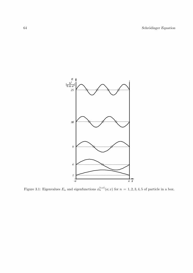
The wave functions represent stationary states of the particle in a one-dimensional box. The wavefunctions for the five lowest energies En are presented in Fig. (3.1). Notice that the number ofnodes of the wave functions increase by one in going from one state to the state with the nexthigher energy En. By counting the number of their nodes one can determine the energy orderingof the wave functions.It is desirable to normalize the wave functions such that∫ +a

−adx |φ(e,o)

n (a;x)|2 = 1 (3.91)

holds. This condition implies for the even states

|An|2∫ +a

−adx cos2nπx

2a= |An|2 a = 1 , n = 1, 3, 5 . . . (3.92)

and for the odd states

|An|2∫ +a

−adx sin2nπx

2a= |An|2 a = 1 , n = 2, 4, 6 . . . (3.93)

The normalization constants are then

An =

√1a. (3.94)


1

4

9

16

25

-a a x

E

[ ]h2

8 m a2

Figure 3.1: Eigenvalues En and eigenfunctions φ(e,o)n (a;x) for n = 1, 2, 3, 4, 5 of particle in a box.


The Stationary States form a Complete Orthonormal Basis of F1

We want to demonstrate now that the set of solutions (3.89, 3.90, 3.94)

B1 = φn(a;x) , n = 1, 2, 3, . . . (3.95)

where

φn(a;x) =

√1a

cosnπx2a for n = 1, 3, 5 . . .sinnπx2a for n = 2, 4, 6 . . .

(3.96)

together with the scalar product5

〈f |g〉Ω1 =∫ +a

−adxf(x) g(x) , f, g ∈ F1 (3.97)

form an orthonormal basis set, i.e., it holds

〈φn|φm〉Ω1 = δnm . (3.98)

The latter property is obviously true for n = m. In case of n 6= m we have to consider three cases,(i) n,m both odd, (ii) n,m both even, and (iii) the mixed case. The latter case leads to integrals

〈φn|φm〉Ω1 =1a

∫ +a

−adx cos

nπx

2asin

mπx

2a. (3.99)

Since in this case the integrand is a product of an even and of an odd function, i.e., the integrandis odd, the integral vanishes. Hence we need to consider only the first two cases. In case of n,modd, n 6= m, the integral arises

〈φn|φm〉Ω1 = 1a

∫ +a−a dx cosnπx2a cosmπx2a =

1a

∫ +a−a dx

[cos (n−m)πx

2a + cos (n+m)πx2a

](3.100)

The periods of the two cos-functions in the interval [−a, a] are N, N ≥ 1. Obviously, the integralsvanish. Similarly, one obtains for n,m even

〈φn|φm〉Ω1 = 1a

∫ +a−a dx sinnπx2a sinmπx2a =

1a

∫ +a−a dx

[cos (n−m)πx

2a − cos (n+m)πx2a

](3.101)

and, hence, this integral vanishes, too.Because of the property (3.98) the elements of B1 must be linearly independent. In fact, for

f(x) =∞∑n=1

dn φn(a;x) (3.102)

holds according to (3.98)

〈f |f〉Ω1 =∞∑n=1

d2n . (3.103)

5We will show in Section 5 that the property of a scalar product do indeed apply. In particular, it holds:〈f |f〉Ω1 = 0 → f(x) ≡ 0.


f(x) ≡ 0 implies 〈f |f〉Ω1 = 0 which in turn implies dn = 0 since d2n ≥ 0. It follows that B1

defined in (3.95) is an orthonormal basis.We like to show finally that the basis (3.95) is also complete, i.e., any element of the function spaceF1 defined in (3.78) can be expressed as a linear combination of the elements of B1 defined in(3.95, 3.96). Demonstration of completeness is a formidable task. In the present case, however,such demonstration can be based on the theory of Fourier series. For this purpose we extend thedefinition of the elements of F1 to the whole real axis through

f : R → R ; ~f(x) = f([x+ a]a − a) (3.104)

where [y]a = ymod2a. The functions f are periodic with period 2a. Hence, they can be expandedin terms of a Fourier series, i.e., there exist real constants an, n = 0, 1, 2, . . . and bn, n = 1, 2, . . .such that

f =∞∑n=0

an cosnπx

2a+

∞∑n=1

an sinnπx

2a(3.105)

The functions f corresponding to the functions in the space F1 have zeros at x = ±ma, m =1, 3, 5 . . . Accordingly, the coefficients an, n = 2, 4, . . . and bn, n = 1, 3, . . . in (3.105) must vanish.This implies that only the trigonometric functions which are elements of B1 enter into the Fourierseries. We have then shown that any f corresponding to elements of F1 can be expanded in termsof elements in B1. Restricting the expansion (3.105) to the interval [−a, a] yields then also anexpansion for any element in F1 and B1 is a complete basis for F1.

Evaluating the Propagator

We can now use the expansion of any initial wave function ψ(x, t0) in terms of eigenfunctionsφn(a;x) to obtain an expression for ψ(x, t) at times t > t0. For this purpose we expand

ψ(x, t0) =∞∑n=1

dn φn(a;x) . (3.106)

Using the orthonormality property (3.98) one obtains∫ +a

−adx0φm(a;x0)ψ(x0, t0) = dm . (3.107)

Inserting this into (3.106) and generalizing to t ≥ t0 one can write

ψ(x, t) =∞∑n=1

φn(a;x) cn(t)∫ +a

−adx0φn(a;x0)ψ(x0, t0) (3.108)

where the functions cn(t) are to be determined from the Schrodinger equation (3.79) requiring theinitial condition

cn(t0) = 1 . (3.109)

Insertion of (3.108) into the Schrodinger equation yields∑∞n=1 φn(a;x) ∂tcn(t)

∫ +a−a dx0φn(a;x0)ψ(x0, t0) =∑∞

n=1

(− i~En)φn(a;x) cn(t)

∫ +a−a dx0φn(a;x0)ψ(x0, t0) . (3.110)


Multiplying both sides by φm(a;x) and integrating over [−a, a] yields, according to (3.98),

∂t cm(t) = − i~

Em cm(t) , cm(t0) = 1 . (3.111)

The solutions of these equations which satisfy (3.109) are

cm(t) = exp(− i~

Em (t − t0)). (3.112)

Equations (3.108, 3.112) determine now ψ(x, t) for any initial condition ψ(x, t0). This solution canbe written

ψ(x, t) =∫ +a

−adx0 φ(x, t|x0, t0)ψ(x0, t0) (3.113)

where

φ(x, t|x0, t0) =∞∑n=1

φn(a;x) exp(− i~

En (t − t0))φn(a;x0) . (3.114)

This expression has the same form as postulated in the path integral formulation of QuantumMechanics introduced above, i.e., in (2.5). We have identified then with (3.114) the representationof the propagator for a particle in a box with infinite walls.It is of interest to note that φ(x, t|x0, t0) itself is a solution of the time-dependent Schrodingerequation (3.79) which lies in the proper function space (3.78). The respective initial conditionis φ(x, t0|x0, t0) = δ(x − x0) as can be readily verified using (3.113). Often the propagatorφ(x, t|x0, t0) is also referred to as a Greens function. In the present system which is composedsolely of bound states the propagator is given by a sum, rather than by an integral (3.54) as in thecase of the free particle system which does not exhibit any bound states.Note that the propagator has been evaluated in terms of elements of a particular function space F1,the elements of which satisfy the appropriate boundary conditions. In case that different boundaryconditions hold the propagator will be different as well.

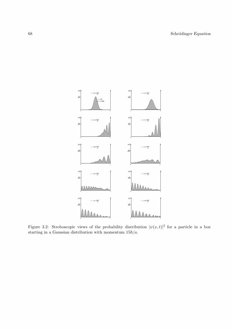
Example of a Non-Stationary State

As an illustration of a non-stationary state we consider a particle in an initial state

ψ(x0, t0) =[

12πσ2

] 14

exp(− x2

0

2σ2+ i k0 x0

), σ =

a

4, k0 =

15a. (3.115)

This initial state corresponds to the particle being localized initially near x0 = 0 with a velocityv0 = 15~/ma in the direction of the positive x-axis. Figure 3.2 presents the probability distributionof the particle at subsequent times. One can recognize that the particle moves first to the left andthat near the right wall of the box interference effects develop. The particle moves then to theleft, being reflected at the right wall. The interference pattern begins to ‘smear out’ first, but thecollision with the left wall leads to new interference effects. The last frame shows the wave frontreaching again the right wall and the onset of new interference.


-a a

1π σ

|Ψ|2

k = 15a

-a a

1π σ

|Ψ|2

-a a

1π σ

|Ψ|2

-a a

1π σ

|Ψ|2

-a a

1π σ

|Ψ|2

-a a

1π σ

|Ψ|2

-a a

1π σ

|Ψ|2

-a a

1π σ

|Ψ|2

-a a

1π σ

|Ψ|2

-a a

1π σ

|Ψ|2

h2m a2

t = 0.00

h2m a2

t = 0.48

h2m a2

t = 0.96

h2m a2

t = 1.92h2

m a2t = 2.16

h2m a2

t = 1.68

h2m a2

t = 1.20

h2m a2

t = 0.72

h2m a2

t = 0.24

h2m a2

t = 1.44

Figure 3.2: Stroboscopic views of the probability distribution |ψ(x, t)|2 for a particle in a boxstarting in a Gaussian distribution with momentum 15~/a.

3.6: Particle in Three-Dimensional Box 69

Summary: Particle in One-Dimensional Box

We like to summarize our description of the particle in the one-dimensional box from a point ofview which will be elaborated further in Section 5. The description employed a space of functionsF1 defined in (3.78). A complete basis of F1 is given by the infinite set B1 (3.95). An importantproperty of this basis and, hence, of the space F1 is that the elements of the basis set can beenumerated by integer numbers, i.e., can be counted. We have defined in the space F1 a scalarproduct (3.97) with respect to which the eigenfunctions are orthonormal. This property allowed usto evaluate the propagator (3.114) in terms of which the solutions for all initial conditions can beexpressed.

3.6 Particle in Three-Dimensional Box

We consider now a particle moving in a three-dimensional rectangular box with side lengths2a1, 2a2, 2a3. Placing the origin at the center and aligning the x1, x2, x3–axes with the edgesof the box yields spatial boundary conditions which are obeyed by the elements of the functionspace

F3 = f : Ω → R, f continuous, f(x1,x2,x3) = 0 ∀ (x1,x2,x3)T ∈ ∂ . (3.116)

where Ω is the interior of the box and ∂Ω its surface

Ω = [−a1, a1]⊗ [−a2, a2]⊗ [−a3, a3] ⊂ R3

∂Ω = (x1, x2, x3)T ∈ Ω, x1 = ±a1 ∪ (x1, x2, x3)T ∈ Ω, x2 = ±a2∪ (x1, x2, x3)T ∈ Ω, x3 = ±a3 . (3.117)

We seek then solutions of the time-dependent Schrodinger equation

i~∂tψ(x, t) = H ψ(x1, x2, x3, t) , H = − ~2

2m(∂2

1 + ∂22 + ∂2

3

)(3.118)

which are stationary states. The corresponding solutions have the form

ψ(x1, x2, x3, t) = exp(− i~

E t

)φE(x1, x2, x3) (3.119)

where φE(x1, x2, x3) is an element of the function space F3 defined in (3.116) and obeys the partialdifferential equation

H φE(x1, x2, x3) = E φE(x1, x2, x3) . (3.120)

Since the Hamiltonian H is a sum of operators O(xj) each dependent only on a single variable, i.e.,H = O(x1) +O(x2) +O(x3), one can express

φ(x1, x2, x3) =3∏j=1

φ(j)(xj) (3.121)

where

− ~2

2m∂2j φ

(j)(xj) = Ej φ(j)(xj) , φ(j)(±aj) = 0 , j = 1, 2, 3 (3.122)


and E1 + E2 + E3 = E. Comparing (3.122) with (3.80) shows that the solutions of (3.122) aregiven by (3.96) and, hence, the solutions of (3.120) can be written

φ(n1,n2,n3)(a1, a2, a3;x1, x2, x3) = φn1(a1;x1)φn2(a2;x2)φn3(a3;x3)n1, n2, n3 = 1, 2, 3, . . . (3.123)

and

E(n1,n2,n3) =~

2π2

8m

(n2

1

a21

+n2

2

a22

+n2

3

a23

), n1, n2, n3 = 1, 2, 3, . . . (3.124)

The same considerations as in the one-dimensional case allow one to show that

B3 = φ(n1,n2,n3)(a1, a2, a3;x1, x2, x3) , n1, n2, n3 = 1, 2, 3, . . . (3.125)

is a complete orthonormal basis of F3 and that the propagator for the three-dimensional box is

φ(~r, t|~r0, t0) =∞∑

n1,n2,n3=1

φ(n1,n2,n3)(a1, a2, a3;~r) (3.126)

exp(− i~

E(n1n2n3) (t − t0))φ(n1,n2,n3)(a1, a2, a3;~r0) .

Symmetries

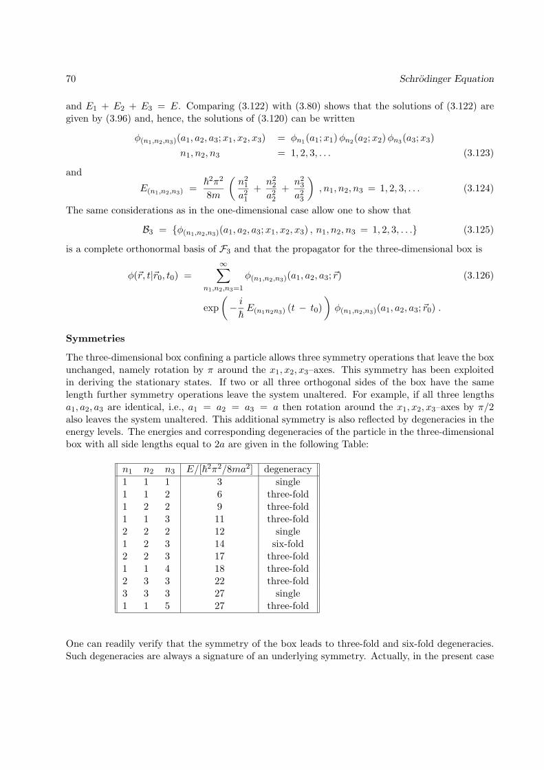
The three-dimensional box confining a particle allows three symmetry operations that leave the boxunchanged, namely rotation by π around the x1, x2, x3–axes. This symmetry has been exploitedin deriving the stationary states. If two or all three orthogonal sides of the box have the samelength further symmetry operations leave the system unaltered. For example, if all three lengthsa1, a2, a3 are identical, i.e., a1 = a2 = a3 = a then rotation around the x1, x2, x3–axes by π/2also leaves the system unaltered. This additional symmetry is also reflected by degeneracies in theenergy levels. The energies and corresponding degeneracies of the particle in the three-dimensionalbox with all side lengths equal to 2a are given in the following Table:

n1 n2 n3 E/[~2π2/8ma2] degeneracy1 1 1 3 single1 1 2 6 three-fold1 2 2 9 three-fold1 1 3 11 three-fold2 2 2 12 single1 2 3 14 six-fold2 2 3 17 three-fold1 1 4 18 three-fold2 3 3 22 three-fold3 3 3 27 single1 1 5 27 three-fold

One can readily verify that the symmetry of the box leads to three-fold and six-fold degeneracies.Such degeneracies are always a signature of an underlying symmetry. Actually, in the present case

3.6: Particle in Three-Dimensional Box 71

‘accidental’ degeneracies also occur, e.g., for (n1, n2, n3) = (3, 3, 3) (1, 1, 5) as shown in the Tableabove. The origin of this degeneracy is, however, the identity 32 + 32 + 32 = 12 + 12 + 52.One particular aspect of the degeneracies illustrated in the Table above is worth mentioning. Weconsider the degeneracy of the energy E122 which is due to the identity E122 = E212 = E221. Anylinear combination of wave functions

φ(~r) = αφ(1,2,2)(a, a, a;~r) + β φ(2,1,2)(a, a, a;~r) + γ φ(2,2,1)(a, a, a;~r) (3.127)

obeys the stationary Schrodinger equation H φ(~r) = E122 φ(~r). However, this linear combinationis not necessarily orthogonal to other degeneraste states, for example, φ(1,2,2)(a, a, a;~r). Hence,in case of degenerate states one cannot necessarily expect that stationary states are orthogonal.However, in case of an n–fold degeneracy it is always possible, due to the hermitian character ofH, to construct n orthogonal stationary states6.

6This is a result of linear algebra which the reader may find in a respective textbook.

The Schr odinger Equation - University of Illinois at Urbana ... 3 The Schr odinger Equation 3.1...

Documents

Transcript of The Schr odinger Equation - University of Illinois at Urbana ... 3 The Schr odinger Equation 3.1...