The role of planarity in connectivity problems ... · The role of planarity in connectivity...

HAL Id: dumas-00854884https://dumas.ccsd.cnrs.fr/dumas-00854884

Submitted on 28 Aug 2013

HAL is a multi-disciplinary open accessarchive for the deposit and dissemination of sci-entific research documents, whether they are pub-lished or not. The documents may come fromteaching and research institutions in France orabroad, or from public or private research centers.

L’archive ouverte pluridisciplinaire HAL, estdestinée au dépôt et à la diffusion de documentsscientifiques de niveau recherche, publiés ou non,émanant des établissements d’enseignement et derecherche français ou étrangers, des laboratoirespublics ou privés.

The role of planarity in connectivity problemsparameterized by treewidth

Julien Baste

To cite this version:Julien Baste. The role of planarity in connectivity problems parameterized by treewidth. DataStructures and Algorithms [cs.DS]. 2013. �dumas-00854884�

https://dumas.ccsd.cnrs.fr/dumas-00854884

https://hal.archives-ouvertes.fr

The role of planarity in connectivity problemsparameterized by treewidth

Julien BasteSupervised by Ignasi Sau

AlGCo project-team, CNRS, LIRMM, Montpellier, [email protected] and [email protected]

Abstract. For some years it was believed that for “connectivity” problems suchas Hamiltonian Cycle, algorithms running in time 2O(tw) ·nO(1) –called single-exponential– existed only on planar and other sparse graph classes, where twstands for the treewidth of the n-vertex input graph. This was recently dis-proved by Cygan et al. [FOCS 2011] and Bodlaender et al. [ICALP 2013], whoprovided single-exponential algorithms on general graphs for essentially all con-nectivity problems that were known to be solvable in single-exponential timeon sparse graphs. During my internship we further investigate the role of pla-narity in connectivity problems parameterized by treewidth, and convey thatseveral problems can indeed be distinguished according to their behavior on pla-nar graphs. In particular, we show that there exist problems that cannot besolved in time 2o(tw log tw) · nO(1) on general graphs but that can be solved intime 2O(tw) · nO(1) when restricted to planar graphs, and problems that can besolved in time 2O(tw log tw) · nO(1) on general graphs but that cannot be solvedin time 2o(tw log tw) · nO(1) even when restricted to planar graphs, the negativeresults holding unless the ETH fails. We feel that our results constitute a firststep in a subject that can be much exploited.

Keywords: parameterized complexity, treewidth, dynamic programming, con-nectivity problems, single-exponential algorithms, planar graphs.

1 Introduction

Motivation and previous work. Graph is a fundamental data structurethat represent elements and relations between them. Studying algorithmsperforming on these graphs is crucial in many fields, networks for example.Many problems on graphs are well known and can be solved in polynomialtime. Shortest Path, which is the problem of finding the shortest pathbetween two given vertices, is an example of problem on graph that can besolved in linear time in the number of vertices of the input graph. On another side, many problems in graph theory are known to be NP-hard. In thisreport we focus only on NP-hard problems. To improve known algorithmson NP-hard problems, a solution is to find a parameter, smaller than the sizeof the graph, and solve problems in function of this parameter. For graphclasses where the parameter is small enough, solving problem in functionof the given parameter improve the time complexity.

The starting point is to see that NP-hard problems are easy to solve intrees. Because of this observation, Robertson and Seymour introduce in [19]

2 Julien Baste Supervised by Ignasi Sau

a graph parameter call treewidth that is a way to measure the distancebetween a given graph and a tree. This parameter becames very interestingwith the apparition of the Courcelle’s theorem in [3]. This theorem statesthat each graph problem that can be expressed in monadic second orderlogic can be solved in time f(tw)·n on a graph with n vertices and treewidthtw. Even if the f function is unavoidably huge [11], this theorem is reallyimportant as it gives a first set of problems that can be solved by usingtreewidth. It is especially important because we know many graph classeswhich have a bounded treewidth. For these graph classes, problem that canbe expressed in monadic second order can be solved in linear time. Thenatural and crucial continuation is to identify problems where the functionf does not grow too fast.

If the input is a n-vertex graph G given with a tree-decompositionof width tw, then we know many problems that can be solved in time2O(tw log tw) ·nO(1). Intuitively, it is the case for problems that can be solvedvia dynamic programming on a tree-decomposition by enumerating all par-titions or packings of vertices in the bags of the tree-decomposition, whichare twtw = 2O(tw log tw) many. In this report, all the problems considered canbe solved in time 2O(tw log tw) ·nO(1). In particular, we are interesting in whichof them can be solved in single-exponential time i.e. in time 2O(tw) · nO(1).Let us discuss on existing works.

It is well known that many problems can be solved in single-exponential.Intuitively it is the case for problems with locally checkable certificates i.e.a certificate that uses a constant size for each vertex and that can be checkby a cardinality check and by iteratively looking at the neighborhood ofthe input graph. Vertex Cover, where we should find a set of verticesof minimum size such that each vertex contains at least an element of thisset, is an example of these problems. For it, we enumerate subsets of thebags of an optimal tree-decomposition, which are 2O(tw), and keep only thesubsets that give a local certificate. In this report, we are looking on prob-lems that have not got locally checkable certificates. More precisely, we areinteresting to the class of connectivity problems which contains problemssuch as Hamiltonian cycle, Steiner Tree, or Connected VertexCover. These problems are called like that because the solution shouldsatisfy a connectivity requirement (see [1,4,21] for more details). The longtime used algorithms to solve these problems used classic dynamic pro-gramming techniques that enumerate all partitions or packings of the bagsof the tree-decomposition.

A succession of paper shows that, when restricted to sparse graphs,many of these connectivity problems can be solved in single-exponentialtime. It is the case for planar graphs [10], graphs with bounded genus [7,21],and graphs excluding a fixed graph as a minor [9,22]. The idea below these

The role of sparsity in connectivity problems parameterized by treewidth 3

improvements is to use a special type of branch-decompositions (which areobjects similar to tree-decompositions) that has nice combinatorial proper-ties. These properties lie on the fact that graphs are sparse.

Improvement in this field was blocked at this stage during a long time.The common belief is that, on general graphs, only problems with locallycheckable certificates can be solved in single-exponential time. This be-lief was amplified with the proof, by Lokshtanov et al. [17], that DisjointPaths, a connectivity problem, cannot be solved in 2o(tw log tw)·nO(1) on gen-eral graph under the exponential time hypothesis. Cygan et al. [4] broke thisbelief with a single-exponential randomize algorithm, called Cut&Count,that solved connectivity problems like Longest Path, Feedback Ver-tex Set, or Connected Vertex Cover on general graph. Bodlaenderet al. [1] still improved it by exhibiting another single-exponential deter-ministic algorithm that basicaly solves the same problems So we arrive at apoint where all connectivity problems that are single-exponential on sparsegraph classes [7, 9, 10, 21, 22] are also solvable in single-exponential timeon general graphs [1, 4], and we have not got any example of case wheresparsity improves the algorithm time.

Our results. At this stage, we could suppose that sparsity is not an inter-esting restriction for obtaining single-exponential algorithms. In this article,we highlight that sparsity, especially planarity, does play a role in connec-tivity problems parameterized by treewidth. For connectivity problems thatcan be solved in time 2O(tw log tw) · nO(1) in general graph, we distinct threedisjoint types:

• Type 1: Problems that can be solved in time 2O(tw) · nO(1) on generalgraphs.• Type 2: Problems that cannot be solved in time 2o(tw log tw) · nO(1) on

general graphs (up to some reasonable complexity assumption), but thatcan be solved in time 2O(tw) · nO(1) when restricted to planar graphs.• Type 3: Problems that cannot be solved in time 2o(tw log tw) ·nO(1) even

when restricted to planar graphs.

Our main contribution is to show that Type 2 and Type 3 are non-empty.It permits to distinct connectivity problems not only on their behaviourson general graphs but also on their behaviours on planar graphs. Moreprecisely, we prove the following results:

– For many problems with locally checkable certificates, it is known thatsingle-exponential time algorithms are the best we can do unless theETH fails [14]. These lower bounds are proved for general graphs andeach problem need an ad-hoc proof. We prove, in Section 4, that Pla-nar 3-colorability, which is a problem of Type 1, cannot be solved


in time 2o(tw) · nO(1) unless the ETH fails, even when the planar inputgraph has maximum degree at most 5.

– We reuse Cycle Packing, Max Cycle Cover, and MaximallyDisconnected Dominating Set that are prove in [4] to be unsolvablein time 2o(tw log tw) ·nO(1) unless ETH fails. We prove that these problemsare of type 2. In Section 5 we focus on Planar Cycle Packing andprove that it can be solved in time 2O(tw) ·nO(1) but cannot be solved in2o(tw) · nO(1) unless ETH fails.

– In Section 6, we introduce Monochromatic Disjoint Paths, a vari-ant of the Disjoint Paths problem on a vertex-colored graph with ad-ditional color restrictions for the paths, and prove that this problem is ofType 3. We exhibit an algorithm solving Monochromatic DisjointPaths in time 2O(tw log tw) · nO(1) and show that Planar Monochro-matic Disjoint Paths cannot be solved in time 2o(tw log tw) · nO(1).

Section 2 is dedicated to preliminaries. We introduce global ideas ofprevious works in Section 3. Section 4, Section 5, and Section 6 are dedicatedrespectively to problems of Type 1, Type 2, and Type 3. We add in Section 7a lower bound for Planar Subgraph Isomorphism that uses the sameideas than the reduction of Planar Monochromatic Disjoint Pathsand in Section 8 a lower bound for Planar Disjoint Paths that uses thesame ideas than the reduction of Planar Cycle Packing. We finish inSection 9 by highlighting some further investigations that can be done.

2 Preliminaries

Exponential time hypothesis. The Exponential time hypothesis. is the hy-pothesis that 3-SAT cannot be solved in subexponential time. We use ETHas a shortcut for Exponential time hypothesis.

Sets. We use the notation [n] for the set {1, . . . , n}. In the set [k] × [k], arow is a set {i} × [k] and a column is a set [k]× {i} for some i ∈ [k].

Graphs. For any graph-theoretic notation not defined here, the reader isreferred to [5]. A graph G is a pair (V,E) where V is the set of verticesof G and E ⊆ V × V is the set of edges. All the considered graphs areundirected and contain neither loops nor multiple edges. We denote byV (G) the set of vertices of the graph G and by E(G) its set of edges. Whenthe context is clear, n stands for the number of vertices of a graph G,which will typically be the input graph of the problem under consideration.A subgraph H = (VH , EH) of a graph G = (V,E) is a graph such thatVH ⊆ V and EH ⊆ E ∩ (VH × VH). The degree of a vertex v in a graph Gdenoted by degG(v), is the number of edges of G containing v.


A grid m∗k is a graph Grm,k = ({ai,j|i ∈ [m], j ∈ [k]}, {{ai,j, ai+1,j}|i ∈[m− 1], j ∈ [k]} ∪ {{ai,j, ai,j+1}|i ∈ [m], j ∈ [k − 1]}). When m = k we justspeak about a grid of size k.

We say that there is a path s . . . t in a graph G if there exist m ∈ Nand x0, . . . , xm in V (G) such that x0 = s, xm = t, and for all i ∈ [m],{xi−1, xi} ∈ E(G).

A tree T is a graph with no cycles. In a tree, a leaf is a vertex withdegree 1.

Treewidth. A tree-decomposition of width w of a graph G = (V,E) is a pair(T, σ), where T is a tree and σ = {Bt|Bt ⊆ V, t ∈ V (T )} such that:

–⋃t∈V (T )Bt = V ,

– For every edge {u, v} ∈ E there is a t ∈ V (T ) such that {u, v} ⊆ Bt,– Bi ∩Bk ⊆ Bj for all {i, j, k} ⊆ V (T ) such that j lies on the path i . . . k

in T ,– maxi∈V (T ) |Bt| = w + 1.

The set Bt are called bag. The treewidth of G, denoted tw(G), is thesmallest integer w such that there is a tree-decomposition of G of width w.An optimal tree-decomposition is a tree-decomposition of width tw.

Pathwidth. A path-decomposition of a graph G = (V,E) is a tree-decomposition, (T, σ) such that T is a path. The pathwidth of G, denotedpw(G), is the smallest integer w such that there is a path-decompositionof G of width w. Clearly, for any graph G, we have tw(G) 6 pw(G).

Branchwidth. A branch-decomposition (T, σ) of a graph G = (V,E) consistsof an unrooted ternary tree T and a bijection σ : L → E from the set Lof leaves of T to the edge set of G. We define for every edge e of T themiddle set mid(e) ⊆ V (G) as follows: Let T1 and T2 be the two connectedcomponents of T\{e}. Then let Gi be the graph induced by the edge set{σ(f) : f ∈ L ∩ V (Ti)} for i ∈ {1, 2}. The middle set is the intersectionof the vertex set of G1 and G2, i.e., mid(e) := V (G1) ∩ V (G2). When weconsider T as rooted, we let Ge be the graph Gi such that Ti does notcontain the root of T . The width of (T, σ) is the maximum order of themiddle sets over all edges of T , i.e., w(T, σ) := max{|mid(e)||e ∈ T}. Thebranchwidth of G, denoted bw(G), is the minimum width over all branchdecompositions of G. An optimal branch decomposition of G is a branchdecomposition (T, σ) of width bw(G).

The branch-width of a graph G with at least 3 edges is linked totreewidth by the relation from [20]: bw(G)− 1 6 tw(G) 6 b3

2bw(G)c − 1.


Planar graphs. Let Σ be the sphere {(x, y, z) ∈ R3 : x2 + y2 + z2 = 1}. Bya Σ-plane graph G we mean a planar graph G with the vertex set V (G),the edge set E(G), and the face set F (G) drawn without edge crossings inΣ.

An O-arc is a subset of Σ homeomorphic to a circle. An O-arc in Σis called a noose of a Σ-plane graph G if it meets G only in vertices andintersects with every faces at most once. Each noose O bounds two opendiscs ∆1, ∆2 in Σ, i.e., ∆1 ∩∆2 = ∅ and ∆1 ∪∆2 ∪O = Σ.

For a Σ-plane graph G, we define a sphere cut decomposition or sc-decomposition (T, σ, π) of G as a branch decomposition such that for everyedge e of T there exists a noose Oe bounding the two open discs ∆1 and∆2 such that Gi ⊆ ∆i ∪ Oe, 1 6 i 6 2. Thus Oe meets G only in mid(e)and its length is |mid(e)|.

Partition. A partition P of a set S is a set of subset of S such that⋃s∈P s =

S and for all s1, s2 ∈ P , s1 ∩ s2 = ∅. A partition P is called non-crossingmatching if for each s1, s2 ∈ P , for each a, b ∈ s1 and c, d ∈ s2 with a < band c < d then one of the following situations occurred: a < b < c < d,a < c < d < b, c < d < a < b, or c < a < b < d. Kreweras showed in [15]that the number of non-crossing partition on [k] for k ∈ N is at most 4k.

Matchings. A matching M is a set of pair, also call edges, such that foreach e, e′ ∈ M , e 6= e′, e ∩ e′ = ∅. For a matching M in a graph G, wedenote by V [M ] the set of all vertices that belong to an edge of M . We saythat two matchings M and M ′ are disjoint if V [M ] ∩ V [M ′] = ∅.

A matching M on V = {v1, . . . , vn}, for some n ∈ N∗, is called non-crossing matching if for each {va, vb}, {vc, vd} ∈ M , with a < b and c < d,then one of the following situations occurred: a < b < c < d, a < c < d < b,c < d < a < b, or c < a < b < d.

Kreweras showed in [15] that the number of non-crossing matchings on[k] for k ∈ N is at most 2k.

Planar problem. Let P be a problem defined on graphs. We denote byPlanar P the restriction of the problem P to the case where the inputgraphs are restricted to be planar.

3 Algorithms in 2O(tw) · nO(1) for connectivityproblems

3.1 On planar graphs

Let us present the work of Dorn et al. In [10], they present how to solvethe majority of the planar connectivity problems in time 2O(tw) · nO(1). For


these algorithms, we use a special branch-decomposition, the sphere cutdecomposition, that has nice combinatorial properties. Let G = (V,E) agraph given with its planar embedding and let (T, σ, π) be the sphere cutdecomposition of the graph G. Let e be an edge of T then we can draw acircle, called noose, that meets G only in vertices and intersects with everyfaces at most once. Each noose Oe bounds two open discs ∆1, ∆2 in Σ, i.e.,∆1∩∆2 = ∅ and ∆1∪∆2∪O = Σ such that Gi ⊆ ∆i∪Oe, 1 6 i 6 2. ThusOe meets G only in mid(e) and its length is |mid(e)|. That means thatfor each cut, we isolate two planar subgraphs of G that we link together.In particular, when performing dynamic programming, when we merge thetwo tables of the two children e1 and e2 of e, these tables correspond totwo planar graphs where we keep information only to the vertices that arein the mid(ei) and we construct an other planar graph (see Fig. 1 for anexample).

This planar property mainly reduce the number of partitions in the cutset we have to consider. Kreweras showed in [15] that the number of non-crossing partitions on [k] for k ∈ N is at most 4k. So when we enumerateall partitions or packing of vertices in the mid(e) for a planar connectivityproblems, we just need to keep 4tw partitions for each mid(e), e ∈ T . Withthis, the complexity analysis of algorithms that we use in the general casegives in the planar case a solution in time 2O(tw log tw) · nO(1).

This technique can be adaped for input graph with bounded genus orthat exclude a graph H as minor. As it uses the structure of the inputgraph, it cannot be generalized to general graphs.

3.2 Cut & Count

The Cut&Count technique [4] is based on Monte-Carlo algorithms and cangive false negative with probability at most 1

2. On the other hand, it cannot

give false positive and solves many connectivity problems in time 2O(tw) ·nO(1). The Cut&Count technique is based on the isolation lemma [18] thatpermits to count objects modulo 2 since if we have many solutions to aproblem, it reduces them to a unique one with a high probability.

Definition 1 A function ω : U → Z isolates a set family F ⊆ 2U if thereis a unique S ∈ F with ω(S) = mins∈S(S), with the notation ω(X) =Σu∈Xω(u).

Definition 2 (Isolation Lemma) Let F ⊆ 2U be a set family over auniverse U with |F| > 0. For each u ∈ U , choose a weight ω(u) ∈ {1...N}uniformly and independently at random. Then

Prob[ω isolate F ] > 1− U

N


The planar graph Ge1 . The planar graph Ge2 .

The vertices still not compute

mid(e1) mid(e2)

mid(e)

Fig. 1. An illustration of a use of sphere cut decomposition.

Let S ⊆ 2U be a set of solution, we want to know if this set is empty.As its name says, the Cut&Count technique is based on two parts :

The Cut part: We relax the connectivity requirement so we take a set Rof all possible connected candidate solutions so S ⊆ R. We also considerthe set C of pairs (X,C) where X ∈ R and C is a consistent cut of X.

The Count part: We compute |C| modulo 2 using a sub-procedure. Non-connected candidate solutions X ⊆ R\S are canceled since they areconsistent with an even number of cuts. Connected candidates X ∈ Sremain.

Note that we use the isolation lemma to obtain an odd number of solu-tions in order to make the counting part work.

3.3 rank based and Square determinant algorithms

The Cut&Count technique has several disadvantages. First, it is a prob-abilistic solution, we cannot be confident in the result. Second, they donot extend to counting the number of witnesses. Third, they do not giveintuition for the optimal substructure or equivalence classes. Cut&Counttechnique is an hope to deterministic algorithms working faster than


2O(tw log tw) · nO(1). The first idea is to derandomize Cut&Count but it re-quieres to derandomize the isolation lemma that remains a big open ques-tion.

In [1], authors get rid of these disadvantages. They use the “rank based”and the “determinant” approaches that permit to remove weight and count-ing versions problems that appear in Cut&Count. Removing disadvantageshas a price and the runtime is slightly worse.

The main idea to the rank based approach is, given a graph G and tree-decomposition (T, σ), to define for each bags of the tree-decomposition arepresentative set such that it is enough to enumerate only these represen-tative elements and such that they are 2O(tw) many. For it, authors definefew operations and prove that if we can solve a problem with a dynamicprogramming algorithm that uses only these operations then, we can findfor each bag of the tree-decomposition a representative set of size 2O(tw)

and so, we can solve the considered problem in time 2O(tw) · nO(1).In an other hand, if the goal is to compute the number of solution to

a given connectivity problem, the determinant approach is more adapted.The key idea is to define for a graph G a matrix A that has the mainproperty that if G is a tree then |det(A)| = 1 else det(A) = 0. With thisobservation, to count the number of solutions of our connectivity problem,we bring the count of the number of solutions to the count of the numberof some trees.

4 Tight Problems of Type 1

In this section we show that Planar 3-colorability cannot be solvedin time 2o(tw) · nO(1) even when the input graph has maximum degree atmost 5. It is a commun belief that NP-hard problems parametrized by twcannot be solved in time 2o(tw) · nO(1), assuming some standard complexityassumtion. By making reduction that preserved subexponential complexity,the lower bound 2o(tw) · nO(1) was proved in [14] for problems such that k-Colorability, k-Set Cover, Independent Set, or Vertex Coverassuming ETH. For these reductions the main point is that the relevantparameters should not increase more than linearly. To our best knowledge,there is no such reduction for Planar 3-colorability or Planar Cy-cle Packing. We show that there is a reduction where the parameterincreases quadratically which turn out to be enough for proving an expo-nential lower bound in the treewidth.3-colorabilityInput: A graph G = (V,E).Question: Is there a color function c : V → {1, 2, 3} suchthat for all {x, y} ∈ E, c(x) 6= c(y).


u′u

The gadget.

u C u′

The representation.

Fig. 2. Color gadget.

u

u′

v′v

The gadget.

u

u′

v CC v′

The representation.

Fig. 3. Cross-color gadget.

Theorem 1. Planar 3-colorability cannot be solved in time 2o(√n) ·

nO(1) unless the ETH fails even when the input graph is restricted to havemaximum degree at most 5.

Proof: For the reduction, we need some planar gadgets. The first one isdepicted in Fig. 2 and named C-gadget. This gadget ensures that two ver-tices u and u′ are in the same color class. Note that we can extend theC-gadget for three vertices u, u′, and u′′ and ensure the three vertices tobe in the same color class by fixing a C-gadget between u and u′ and another C-gadget between u′ and u′′. The second one is depicted in Fig. 3 andnamed CC-gadget. In this gadget, introduced in [13], we can check that ifu, v, u′ and v′ are in the same face and oriented in this order around theface, that u and u′ are in the same color class and v and v′ are in the samecolor class.

We reduce from 3-colorability. Let G = (V,E) be a general graphwith V = {v1, . . . , vn} and let n = |V |. We proceed to construct a planargraph H.


CC

CC

CC

CC

CC CC

C

C

C

C

uH,1

vH,1

uH,2

vH,2

uH,3

vH,3

uH,4

vH,4

wH,1

wH,2

wH,3

wH,4

αH,1,2

βH,1,2

αH,1,3

βH,1,3

αH,1,4

βH,1,4

αH,2,3

βH,2,3

αH,2,4

βH,2,4

αH,3,4

βH,3,4

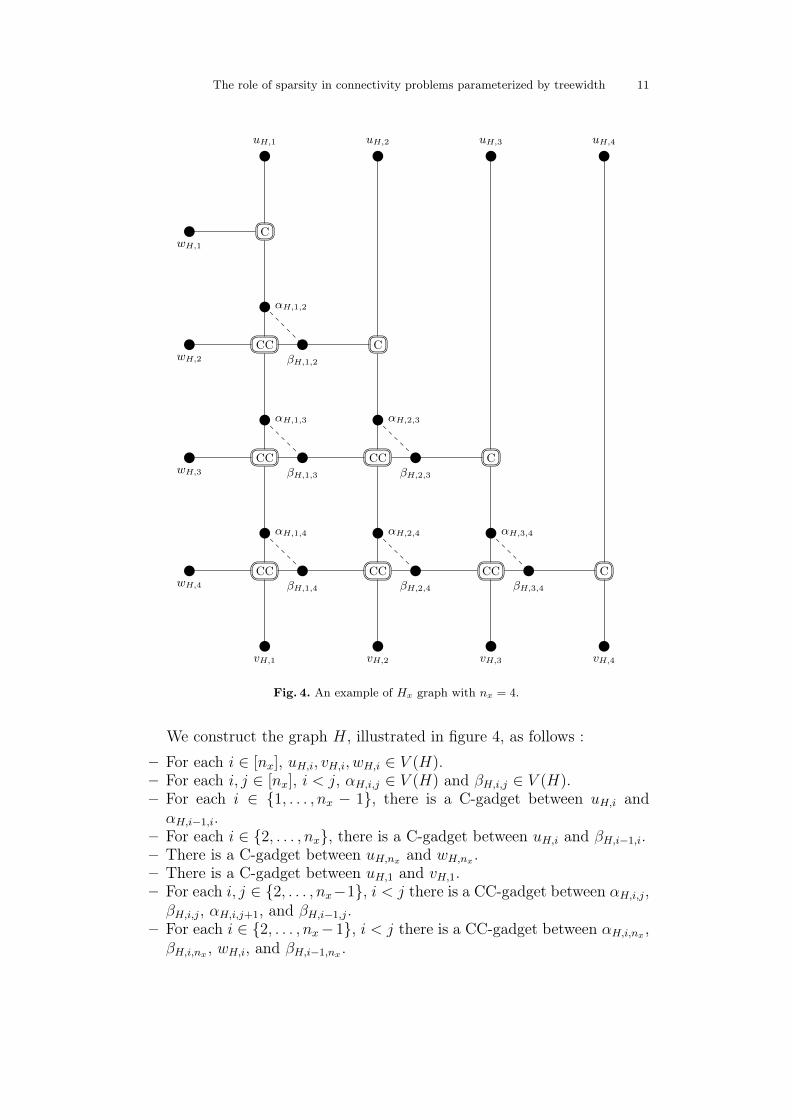
Fig. 4. An example of Hx graph with nx = 4.

We construct the graph H, illustrated in figure 4, as follows :

– For each i ∈ [nx], uH,i, vH,i, wH,i ∈ V (H).– For each i, j ∈ [nx], i < j, αH,i,j ∈ V (H) and βH,i,j ∈ V (H).– For each i ∈ {1, . . . , nx − 1}, there is a C-gadget between uH,i andαH,i−1,i.

– For each i ∈ {2, . . . , nx}, there is a C-gadget between uH,i and βH,i−1,i.– There is a C-gadget between uH,nx and wH,nx .– There is a C-gadget between uH,1 and vH,1.– For each i, j ∈ {2, . . . , nx−1}, i < j there is a CC-gadget between αH,i,j,βH,i,j, αH,i,j+1, and βH,i−1,j.

– For each i ∈ {2, . . . , nx−1}, i < j there is a CC-gadget between αH,i,nx ,βH,i,nx , wH,i, and βH,i−1,nx .


The original node. The simulation of the same node but with locally maximal degree 5.

Fig. 5. Maximal degree diminution to 5.

– For each j ∈ {2, . . . , nx− 1}, i < j there is a CC-gadget between αH,1,j,βH,1,j, αH,1,j+1, and vH,j.

– There is a CC-gadget between αH,1,nx , βH,1,nx , wH,1, and vH,nx .– For each i, j ∈ [nx], i < j, if (vi, vj) ∈ E, then (αH,i,j, βH,i,j) ∈ E(H).

Note that H is planar as the C-gadget and the CC-gadget are planarand we can keep the planarity when building H as Fig. 4 shows.

Because of the properties on the C-gadget and the CC-gadget, for eachi in [n], uH,i, vH,i, and wH,i are in the same color class. Because of the edges(αH,i,j, βH,i,j), if there is an edge between vi and vj in G, then uH,i and uH,jshould receive different colors. If we have a 3-coloring of G then by coloringuH,i with the color of vi for each i ∈ [n] then we find a 3-coloring of H. Ifwe have a coloring of H we color each vi of V with the color of uH,i for eachi ∈ [n].

Let us argue about the maximal degree of the graph H. With the pre-vious construction, the maximal degree in 7. To restrict it to 5, we need toinsert two color gadgets as show in figure 5 for each node with degree 6 or7.

Let us argue about the number of vertices of H. H is a grid of size nwhere each node is replace by a C-gadget, a CC-gadget, or is removed.As these two gadgets have at most 13 vertices, and in the worst case, allthese new vertices have degree 7 and we need to replace them by twocolor gadgets, that have 7 vertices, to reduce to a degree 5, we have that|V (H)| 6 65 · n2. As [14] prove that 3-colorability cannot be solved intime 2o(n) · nO(1), the theorem follow. �

Corollary 1. Planar 3-colorability cannot be solved in time 2o(tw) ·nO(1) unless the ETH fails, where tw stands for the treewidth of the inputgraph even when the input graph is restricted to have maximum degree atmost 5.


Proof: As a planar graph G on n vertices satisfies tw(G) = O(√n) [12],

an algorithm in time 2o(tw) · nO(1) for Planar 3-colorability impliesthat there is an algorithm in time 2o(

√n) · nO(1), which is impossible by

Theorem 4 unless the ETH fails. �

5 Problems of Type 2

In this section we prove that there exist problems of Type 2. More precisely,we prove that Cycle Packing, Max Cycle Cover, Maximally Dis-connected Dominating Set, and Maximally Disconnected Ver-tex Cover are of Type 2.

5.1 The upper bound for Planar Cycle Packing

Cycle PackingInput: A graph G = (V,E) and an integer `0.Parameter: The treewidth tw of G.Question: Does G contain `0 pairwise vertex-disjoint cycles?

Theorem 2. The Planar Cycle Packing problem can be solved in time2O(tw) · nO(1).

Proof: We strongly follow the techniques introduced in [8,10,21,22], whichare based on Catalan structures.

Let G be a graph, X ⊆ V (G), and M a matching on V (G)\X. Intu-itively, M represents the endpoints of the paths we are building and Xis the set of vertices that are already inside a path but they are not anendpoint of any path. We define G[(X,M, `)] = (V [M ],M). We say thatG[(X1,M1, `1), (X2,M2, `2)] is defined if X1 ∩ (X2 ∪ V [M2]) = X2 ∩ (X1 ∪V [M1]) = ∅ and we define G[(X1,M1, `1), (X2,M2, `2)] = G[(X1,M1, `1)] ∪G[(X2,M2, `2)]. Otherwise, we say that G[(X1,M1, `1), (X2,M2, `2)] is un-defined. We say that cp(G,X,M) > ` if G contains paths joining each pairof vertices given by M and ` cycles, all pairwise vertex-disjoint.

We now consider G = (V,E) to be our Σ-plane input graph and `0 ourinteger. Let (T, µ, π) be a sc-decomposition of G of width bw. As in [10], weroot T by arbitrarily choosing an edge e and we subdivide it by inserting anew node s. Let e′ and e′′ be the new edges and set mid(e′) = mid(e′′) =mid(e). We create a new node root r, we connect it to s, by an edge er,and set mid(er) = ∅. The root er is not consider as a leaf.

Let e ∈ E(T ) and Re = {(X,M, `)|X ⊆ mid(e), M is a matchingof a subset of mid(e)\X and cp(Ge, X,M) > `}. We observe that there


ui,1

ci

ui,3

bi

ai

ui,2

ui,0

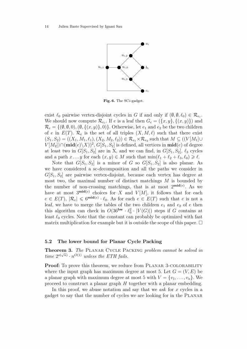
Fig. 6. The SCi-gadget.

exist `0 pairwise vertex-disjoint cycles in G if and only if (∅, ∅, `0) ∈ Rer .We should now compute Rer . If e is a leaf then Ge = ({x, y}, {(x, y)}) andRe = {(∅, ∅, 0), (∅, {(x, y)}, 0)}. Otherwise, let e1 and e2 be the two childrenof e in E(T ). Re is the set of all triples (X,M, `) such that there exist(S1, S2) = ((X1,M1, `1), (X2,M2, `2)) ∈ Re1×Re2 such thatM ⊆ ((V [M1]∪V [M2])∩(mid(e)\X))2, G[S1, S2] is defined, all vertices in mid(e) of degreeat least two in G[S1, S2] are in X, and we can find, in G[S1, S2], `3 cyclesand a path x . . . y for each (x, y) ∈M such that min(`1 + `2 + `3, `0) > `.

Note that G[S1, S2] is a minor of G so G[S1, S2] is also planar. Aswe have considered a sc-decomposition and all the paths we consider inG[S1, S2] are pairwise vertex-disjoint, because each vertex has degree atmost two, the maximal number of distinct matchings M is bounded bythe number of non-crossing matchings, that is at most 2mid(e). As wehave at most 3mid(e) choices for X and V [M ], it follows that for eache ∈ E(T ), |Re| 6 6mid(e) · `0. As for each e ∈ E(T ) such that e is not aleaf, we have to merge the tables of the two children e1 and e2 of e thenthis algorithm can check in O(36bw · `20 · |V (G)|) steps if G contains atleast `0 cycles. Note that the constant can probably be optimized with fastmatrix multiplication for example but it is outside the scope of this paper.�

5.2 The lower bound for Planar Cycle Packing

Theorem 3. The Planar Cycle Packing problem cannot be solved intime 2o(

√n) · nO(1) unless the ETH fails.

Proof: To prove this theorem, we reduce from Planar 3-colorabilitywhere the input graph has maximum degree at most 5. Let G = (V,E) bea planar graph with maximum degree at most 5 with V = {v1, . . . , vn}. Weproceed to construct a planar graph H together with a planar embedding.

In this proof, we abuse notation and say that we ask for x cycles in agadget to say that the number of cycles we are looking for in the Planar


v

u′

v′

u

(a) The expel gadget.

u E u′

(b) Its representation.

v

u′

u′′

v′

u

(c) The double-expel gadget.

Fig. 7. The expel gadget and the double-expel gadget.

pc4

pc2

pc1 pc3w0w1,1

Ew2,2

w2,1

E

w3,2 w3,1

Ew4,2

w4,1

E

w1,2

The gadget.

pc2

pc4

pc1 PC pc3

The representation.

Fig. 8. Path-crossing gadget.

Cycle Packing problem is increased by x. We will ask for a certain num-ber of cycles in each of the introduced gadgets, which by construction willlead to a set of cycles of maximum cardinality in H.

We start by introducing some gadgets. For each i ∈ [n],corresponding to the vertices v1, . . . , vn of G, we add to Hthe SCi-gadget depicted in Fig. 6. More precisely, SCi =({ai, bi, ci, ui,0, ui,1, ui,2, ui,3}, {(ui,0, ui,1), (ui,0, ui,2), (ui,0, ui,3), (ai, ui,1), (ai, ui,2),(bi, ui,2), (bi, ui,3), (ci, ui,1), (ci, ui,3)}). We ask for a cycle inside this gadget.This cycle imposes that at least one of the vertices {ai, bi, ci}, named aselected vertex of the SCi-gadget, is used by the inner cycle and leavesthe possibility that the two others are free. The intended meaning of eachSCi-gadget is as follows. The three vertices ai, bi, and ci correspond to thethree colors in the 3-coloring of G, namely a, b, and c. If for instance ai


ai

bi

ci

ai,1 bi,1 ci,1

ai,2

bi,2

ci,2

(a) The gadget.

ai

bi

ci

ai,1 bi,1 ci,1

ai,2

bi,2

ci,2

(b) An example.

Fig. 9. Bifurcate gadget: To keep planarity, there is a path-crossing gadget in each edge inter-section.

ai,k

aj,k

bi,k bj,k′

ci,k

cj,k′

Fig. 10. Edge gadget: To keep planarity, there is a path-crossing gadget in each edge intersec-tion.

is a selected vertex for i, it will imply that vertex vi can be colored withcolor a.

Therefore, each SCi-gadget defines the available colors for vertex vi,which we call the color output of vertex vi. In order to construct H thatdefine a valid 3-coloring of G, we need to propagate the color output of vi


as many times as the degree of vi in G. For this, we introduce a gadgetcall bifurcate gadget. Before proceeding to the description of the gadget,let us describe its intended function. The objective is, starting with thevertices ai, bi, and ci of the SCi-gadget, to construct a set of degG(vi)triples {ai,k, bi,k, ci,k} for 1 6 k 6 degG(vi) such that in each triple therewill be again at least one selected vertex, defined by the cycles that wewill construct in the bifurcate gadgets. Note that in the SCi-gadget thechoice of a selected vertex in each triple {ai,k, bi,k, ci,k} naturally defines acolor output for vertex vi. The crucial property of the gadget is that theintersection of the color outputs given by all the triples is non-empty if andonly if the graph H contains enough vertex-disjoint cycles. In other words,the existence of the appropriate number of vertex-disjoint cycles in H willdefine an available color for each vertex vi in G.

We now proceed to the construction of the bifurcate gadget.First we need to introduce three other auxiliary gadgets. The firsttwo ones, called expel and double-expel gadgets, are depicted in Fig.7. Formally, for two vertices u and u′, the expel gadget is de-fined as EGu,u′ = ({u, u′, v, v′}, {(u, v), (u, v′), (u′, v), (u′, v′), (v, v′)}),and we ask for a cycle inside each such expel gadget. This gad-get ensures that if u is in another cycle, then u′ is necessarily usedby the internal cycle and vice-versa. Similarly, the double-expel gad-get for three vertices u, u′, and u′′ is defined as DEGu,u′,u′′ =({u, u′, u′′, v, v′}, {(u, v), (u, v′), (u′, v), (u′′, v′), (u′, u′′), (v, v′)}), and we alsoask for a cycle inside each such gadget. This gadget ensures that if u is inanother cycle, then u′ and u′′ are necessarily used by the internal cycle andthat if u′ or u′′ are in an external cycle, then u is necessarily used by theinternal cycle.

As in our construction the edges of the expel gadgets will cross,we need a gadget that replaces each edge-crossing with a planar sub-graph while preserving the existence of the original edges, in the sensethat each of the crossing edges gets replaced by a path joining the end-vertices of the original edge. This gadget is called path-crossing gadgetand is depicted in Fig. 8. Formally the path-crossing gadget PCG issuch that {pc1, pc2, pc3, pc4, w0, w1,1, w1,2, w2,1, w2,2, w3,1, w3,2, w4,1, w4,2} ⊆V (PCG), E(PCG) contains two paths pc1, w1,1, w1,2, w0, w3,2, w3,1, pc3 andpc2, w2,1, w2,2, w0, w4,2, w4,1, pc4, and we add four expel gadgets EGw1,1,w2,2 ,EGw2,1,w3,2 , EGw3,1,w4,2 , EGw4,1,w1,2 to PCG. We ask in this gadget only thefour cycles asked by the expel gadgets. This gadget ensures that an externalcycle that contain an edge from a path-crossing gadget should go straight,i.e., for all α ∈ [4], if the cycle arrives at a vertex pcα it should exit bypc(α+1 (mod 4))+1. If a cycle does not respect this property, we say that thecycle turns inside the path-crossing gadget. That is, the gadget preserves


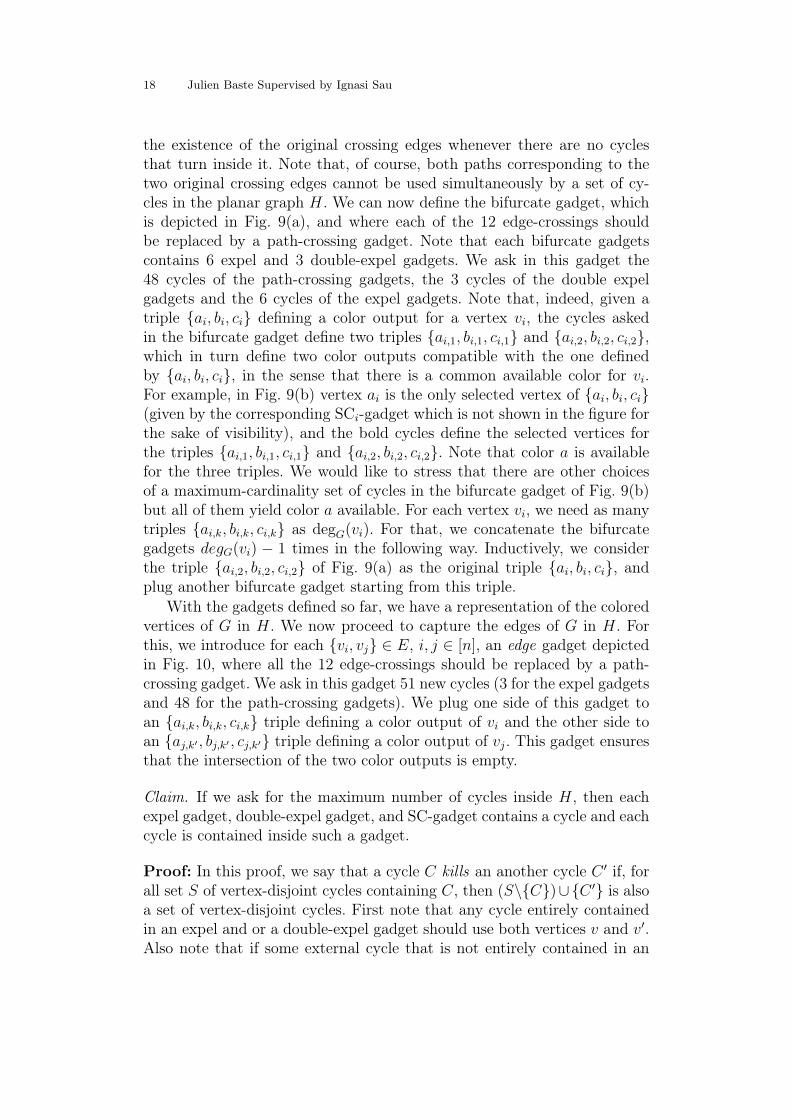
the existence of the original crossing edges whenever there are no cyclesthat turn inside it. Note that, of course, both paths corresponding to thetwo original crossing edges cannot be used simultaneously by a set of cy-cles in the planar graph H. We can now define the bifurcate gadget, whichis depicted in Fig. 9(a), and where each of the 12 edge-crossings shouldbe replaced by a path-crossing gadget. Note that each bifurcate gadgetscontains 6 expel and 3 double-expel gadgets. We ask in this gadget the48 cycles of the path-crossing gadgets, the 3 cycles of the double expelgadgets and the 6 cycles of the expel gadgets. Note that, indeed, given atriple {ai, bi, ci} defining a color output for a vertex vi, the cycles askedin the bifurcate gadget define two triples {ai,1, bi,1, ci,1} and {ai,2, bi,2, ci,2},which in turn define two color outputs compatible with the one definedby {ai, bi, ci}, in the sense that there is a common available color for vi.For example, in Fig. 9(b) vertex ai is the only selected vertex of {ai, bi, ci}(given by the corresponding SCi-gadget which is not shown in the figure forthe sake of visibility), and the bold cycles define the selected vertices forthe triples {ai,1, bi,1, ci,1} and {ai,2, bi,2, ci,2}. Note that color a is availablefor the three triples. We would like to stress that there are other choicesof a maximum-cardinality set of cycles in the bifurcate gadget of Fig. 9(b)but all of them yield color a available. For each vertex vi, we need as manytriples {ai,k, bi,k, ci,k} as degG(vi). For that, we concatenate the bifurcategadgets degG(vi) − 1 times in the following way. Inductively, we considerthe triple {ai,2, bi,2, ci,2} of Fig. 9(a) as the original triple {ai, bi, ci}, andplug another bifurcate gadget starting from this triple.

With the gadgets defined so far, we have a representation of the coloredvertices of G in H. We now proceed to capture the edges of G in H. Forthis, we introduce for each {vi, vj} ∈ E, i, j ∈ [n], an edge gadget depictedin Fig. 10, where all the 12 edge-crossings should be replaced by a path-crossing gadget. We ask in this gadget 51 new cycles (3 for the expel gadgetsand 48 for the path-crossing gadgets). We plug one side of this gadget toan {ai,k, bi,k, ci,k} triple defining a color output of vi and the other side toan {aj,k′ , bj,k′ , cj,k′} triple defining a color output of vj. This gadget ensuresthat the intersection of the two color outputs is empty.

Claim. If we ask for the maximum number of cycles inside H, then eachexpel gadget, double-expel gadget, and SC-gadget contains a cycle and eachcycle is contained inside such a gadget.

Proof: In this proof, we say that a cycle C kills an another cycle C ′ if, forall set S of vertex-disjoint cycles containing C, then (S\{C})∪{C ′} is alsoa set of vertex-disjoint cycles. First note that any cycle entirely containedin an expel and or a double-expel gadget should use both vertices v and v′.Also note that if some external cycle that is not entirely contained in an


expel gadget or a double-expel gadget uses the vertex v or v′ of an expelor a double-expel gadget, then it also use the vertex u (or u and u′′) andwe are not able to find an internal cycle anymore. Therefore, any externalcycle containing v or v′kills the cycle {u, v, v′} or {u′, u′′, v′, v′′}.

Note that if an external cycle of a path-crossing gadget turn in-side it, then without loss of generality it uses a path of the formpc1, w1,1, w1,2, w0, w2,2, w2,1, pc2 inside the path-crossing gadget. This exter-nal cycle kills the cycle inside the expel gadget between w1,1 and w2,2.Moreover, another disjoint external cycle turning in the same path-crossinggadget kills the cycle inside the expel gadget between w3,1 and w4,2.

Let C be a cycle in H that is not contained in only one expel gadget,double-expel gadget, or SCi-gadget. Because of the previous remarks, wehave that C cannot turn in two path-crossing gadgets and if it turns in anypath-crossing gadget then it uses at least two expel or double-expel gadgetsand kills their internal cycles. In both configurations, the introduction of Cin the solution decreases the number of cycles that we can find in H.

The only choice remaining for C is to turn only once in a path-crossinggadget. If it happens inside a bifurcate gadget, then C uses verticesof two expel gadgets expel1 and expel2 corresponding to two differentcolors. The only way to connect vertices corresponding ti different colorsoutside the path-crossing gadget is by using an SCi-gadget. So C killsthe cycles of expel1 and expel2, or it could also use a path leading to anedge gadget. If C turns in a path-crossing gadget inside an edge gadget,then the the analysis is similar but there is an extra case where the edgegadget representing the edge between vi and vj is directly plugged in theSCj-gadget. Just note that in this case none of the vertices {ai, bi, ci} can bea selected vertex with the current set of cycles we ask for„ and therefore inorder to allow it we need to decrease the number of cycles in the solution. �

If we are given a solution of Planar Cycle Packing in H, then foreach i ∈ [n], the selection of a cycle in the SCi-gadget selects a color for vi,that can be any color that is shared by all color outputs of vi, and the edgegadgets ensure that two adjacent vertices are in two different color classes.So in this way we obtain a solution of Planar 3-colorability in G.

Conversely, given a solution of Planar 3-colorability in G, weconstruct a solution of Planar Cycle Packing in H as follows. Foreach i ∈ [n] we choose in the SCi-gadget the cycle of length 4 that con-tains ui,0 and the vertex in {ai, bi, ci} that corresponds to the color of vi.We also choose in the bifurcates gadgets the cycle that select vertices in{ai,1, bi,1, ci,1, ai,2, bi,2, ci,2} that lead to two identical color outputs that isexactly the color output of {ai, bi, ci}. This selection keeps the property thatthe color output of {ai, bi, vi} is contain in the color output of {ai,1, bi,1, ci,1}


and in the color output of {ai,2, bi,2, ci,2}, and leaves free as many verticesas possible for other cycles in other gadgets. Inside the edge gadget repre-senting {vi, vj} ∈ E, we select the three cycles that are allowed by the freevertices. We complete our cycle selection by selecting a cycle in each expelgadget contained in a path-crossing gadget. By the claim, this choice leadsto an optimal solution of Planar Cycle Packing in H.

As the degree of each vertex in G is bounded by 5, the number ofgadgets we introduce for each vi ∈ V (G) to construct H is also boundedby a constant, so the total number of vertices of H is linear in the numberof vertices of G. Therefore if we could solve Planar Cycle Packing intime 2o(

√n) · nO(1) then we could also solve Planar 3-coloring in time

2o(√n) · nO(1), which is impossible by Theorem 1 unless the ETH fails. The

theorem follows. �

From Theorem 3 we obtain the following corollary.

Corollary 2. The Planar Cycle Packing problem cannot be solved intime 2o(tw) · nO(1) unless the ETH fails.

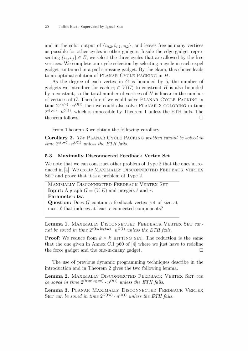
5.3 Maximally Disconnected Feedback Vertex Set

We note that we can construct other problem of Type 2 that the ones intro-duced in [4]. We create Maximally Disconnected Feedback VertexSet and prove that it is a problem of Type 2.

Maximally Disconnected Feedback Vertex SetInput: A graph G = (V,E) and integers ` and r.Parameter: tw.Question: Does G contain a feedback vertex set of size atmost ` that induces at least r connected components?

Lemma 1. Maximally Disconnected Feedback Vertex Set can-not be soved in time 2o(tw log tw) · nO(1) unless the ETH fails.

Proof: We reduce from k × k hitting set. The reduction is the samethat the one given in Annex C.1 p60 of [4] where we just have to redefinethe force gadget and the one-in-many gadget. �

The use of previous dynamic programming techniques describe in theintroduction and in Theorem 2 gives the two following lemma.

Lemma 2. Maximally Disconnected Feedback Vertex Set canbe soved in time 2O(tw log tw) · nO(1) unless the ETH fails.

Lemma 3. Planar Maximally Disconnected Feedback VertexSet can be soved in time 2O(tw) · nO(1) unless the ETH fails.


6 Problems of Type 3

In this section we prove that there exist problems of Type 3. More precisely,we prove that Monochromatic Disjoint Paths is of Type 3. For thisproblem, we need to introduce some definition. Let G = (V,E) be a graph,let k be an integer, and c : V → {0, . . . , k} a color function. Two colors c1and c2 in {0, . . . , k} are compatible and we note c1 ≡ c2 if c1 = 0, c2 = 0, orc1 = c2. Let P = x0 . . . xm be a path inG. We say that P is amonochromaticpath if for all i 6= j, c(xi) and c(xj) are two compatible colors. We letc(P ) = maxi∈[m](c(xi)). We say that P is colored x if x = c(P ). We say thattwo monochromatic paths P and P ′ are color-compatible if c(P ) ≡ c(P ′).

Monochromatic Disjoints PathsInput: A graph G = (V,E) of treewidth tw, acolor function γ : V → {0, . . . , tw}, m ∈ N andN = {Ni = {si, ti}|i ∈ {1, . . . ,m}, si, ti ∈ V }.Parameter: tw.Question: Does G contain m pairwise vertex-disjointmonochromatic paths from si to ti, i ∈ {1, . . . ,m}?

6.1 Algorithm for Monochromatic Disjoint Paths

Lemma 4. Monochromatic Disjoint Paths can be solved in time2O(tw log tw) · nO(1).

Proof: The following algorithm is an adaptation of the algorithm givenin [23] for Disjoint Path.

Let G be a colored graph and let γ : V (G)→ {0, . . . , tw} be the coloringof the graph. Let (Ni = {si, ti})i∈{1...m} be the m paths we are looking forand let (T, µ, π) a sc-decomposition of G of width bw(G). As in [10], weroot T by arbitrarily choosing an edge e and subdivide it by insering anew node s. Let e′ and e′′ be the new edges and set mid(e′) = mid(e′′) =mid(e). Create a new node root r, connect it to s, by an edge er, and setmid(er) = ∅. The root er is not consider as a leaf.

Let now e be an edge of T , let X,P ⊆mid(e) with X∩P = ∅, andM,Lbe two disjoint matchings of mid(e)\(X ∪P ). Let γ0 : P ∪ V [M ]∪ V [L]→{0, . . . , tw} be color functions. Let ϕ : P → {1, . . . ,m} an injectivefunction. Intuitively, we want to keep memories of path inside Ge, soP stands for virtual source of a terminals, M stands for pair of virtualsources that should be links, L stands for pair {x, y} such that there isa path in Ge that link x and y, and X stands for vertices that are al-ready inside a path or both an endpoint and a terminal. We say that


mdp(Ge,mid(e), X, P,M,L, c0, ϕ) = true if all the following conditions arefulfilled.

– For all {si, ti} in N ∩ V (Ge)2

• There exists a monochromatic path si . . . ti in Ge or• There exist {s′i, t′i} ∈M and two monochromatic paths in Ge si . . . s

′i

colored γ0(s′i) and ti . . . t′i colored γ0(t′i) with γ0(s′i) ≡ γ0(t′i).

– For all {si, ti} in N , such that si ∈ V (Ge) and ti 6∈ V (Ge) or vice-versa,• There exist s′i ∈ P such that ϕ(s′i) = i and a monochromatic pathsi = v0 . . . vk = s′i colored c0(s′i).

– For all {xi, yi} in L• There exists a monochromatic path xi . . . yi coloredmax(γ0(xi), γ0(yi)) in Ge.

– All these paths are vertex-disjoint and all vertices in S with degree atleast 2 are in X.

Let S1 = (X1, P1,M1, L1, γ1, ϕ1), and S2 = (X2, P2,M2, L2, γ2, ϕ2) withX1, X2, P1, P2, . . . defined as above. We define G[S1] = (P1 ∪ V [M1] ∪V [L1], {{x, y} ∈ L1}) and colored by γ1 and similarly define G[S2]. We saythat G[S1, S2] is defined if for all x ∈ V (G[S1]) ∩ V (G[S2]), c1(x) ≡ c2(x),X1 ∩ V (G[S2]) = X2 ∩ V (G[S1]) = X1 ∩X2 = ∅, and we define G[S1, S2] =G[S1]∪G[S2] and colored by γ12 defined such that for all x ∈ V (G[S1, S2]),γ12 = max(γ1(x), γ2(x)). Otherwise we say that G[S1, S2] is undefined.

Let e ∈ E(T ), we define Re = {(X,P,M,L, γ, ϕ)|X ⊆ mid(e), P ⊆mid(e), X ∩ P = ∅, M and L are disjoint matchings on mid(e)\(X ∪ P ),V [M ] ∩ V [L] = ∅ and mdp(Ge,mid(e), X, P,M,L, γ, ϕ) = true. We wantto know if (∅, ∅, ∅, ∅, ∅, ∅) ∈ Rer . We can compute Re, for each e ∈ E(T ),as follows :

– if e is a leaf, then Ge = ({x, y}, {(x, y)}• if {x, y} ∈ N thenRe = {({x, y}, ∅, ∅, ∅, ∅, ∅)}• if x ∈ Ni, y ∈ Nj, i 6= j thenRe = {(∅, {x, y}, ∅, ∅, {(x, γ(x)), (y, γ(y))}, {(x, i), (y, j)})}• if x ∈ Ni and ∀j ∈ {1, . . . ,m}, y 6∈ Nj and γ(x) 6≡ γ(y) thenRe = {(∅, {x}, ∅, ∅, {(x, γ(x)}, {(x, i)})}• if x ∈ Ni and ∀j ∈ {1, . . . ,m}, y 6∈ Nj and γ(x) ≡ γ(y) then Re ={(∅, {x}, ∅, ∅, {(x, γ(x)}, {(x, i)}), ({x}, {y}, ∅, ∅, {(y,max(γ(x), γ(y)))}, {(y, i)})}

– if e is not a leaf, let e1 and e2 be the two children of e in E(T ).We construct Re as the set of all 6-uplets (X,P,M,L, γ0, ϕ) suchthat there exist S1 = (X1, P1,M1, L1, γ1, ϕ1) ∈ Re1 , and S2 =(X2, P2,M2, L2, γ2, ϕ2) ∈ Re2 fulfilling the following properties:• H = G[S1, S2] is defined


• For all {xi, yi} in L, there exists a monochromatic path xi . . . yi inH and we have γ0(xi) = γ0(yi) = γ12(xi . . . yi).• All vertices in mid(e) of degree at least 2 in G[S1, S2] are in X.• For all {v, w} in Mi, i ∈ {1, 2}, there is a monochromatic color

compatible path from v to w inG[S1, S2] or two vertices {v′, w′} ∈M ,and two monochromatic color compatible paths v . . . v′ and w . . . w′and we have γ0(v′) = γ0(w

′) = max(γ12(v . . . v′), γ12(w . . . w

′)).• For all i in {1, 2}, For all v in Pi, there exist w ∈ P and a monochro-

matic color compatible path v . . . w or there are w ∈ P3−i such thatϕi(v) = ϕ3−i(w) and a monochromatic path from v . . . w such thatγ0(w) = γ12(v . . . w).• All these paths are pairwise vertex-disjoint.

As in the graph G[S1, S2], by construction, all vertices have degree atmost two, we can check all the previous properties in polynomial timebecause we just have to compare two sets or follow a path in G[S1, S2] tocheck each property. So we can compute each element ofRe in poly(mid(e))steps. As (X,P, V [M ], V [L]) forms a partition of a subset of mid(e), thereare at most 5mid(e) such sets. There are at most tw+ 1 colors and at most(tw + 1)mid(e) choices for γ0. As |{ϕ(x)|x ∈ P}| 6 |P | 6 mid(e), thenthere are at most mid(e)mid(e) such different color functions ϕ possible.As bw − 1 6 tw we have that for all e in E(T ), |mid(e)| 6 tw and so forall e in E(T ), |Re| 6 5tw · (tw + 1)2tw. As for each e ∈ E(T ) such that eis not a leaf, we have to merge the tables of the two children e1 and e2 ofe then the above dynamic programming algorithm can solve Monochro-matic Disjoint Paths in O(25tw · (tw + 1)4tw · |V (G)|) steps. Thelemma follows. Note that the constant can probably be optimized with fastmatrix multiplication for example but it is outside the scope of this paper.�

6.2 Lower bound for Planar Monochromatic Disjoint Paths

Theorem 4. Planar Monochromatic Disjoint Paths cannot besolved in time 2o(pw logpw) · nO(1) unless the ETH fails, where pw standsfor the pathwidth of the input graph.

Proof: We reduce from the k × k hitting set problem. We do not usethe original version but the one considered in [17]:


s

v

t

u

The gadget.

u E v

The representation.

Fig. 11. Expel gadget.

ur,1

ur,2

ur,3

sr

ur,k

vr,0

The gadget.

sr CS vr,0

The representation.

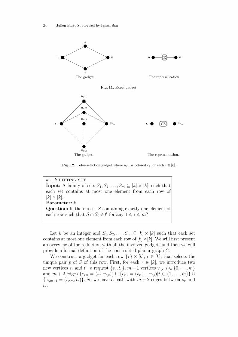
Fig. 12. Color-selection gadget where ur,i is colored ci for each i ∈ [k].

k × k hitting setInput: A family of sets S1, S2, . . . , Sm ⊆ [k] × [k], such thateach set contains at most one element from each row of[k]× [k].Parameter: k.Question: Is there a set S containing exactly one element ofeach row such that S ∩ Si 6= ∅ for any 1 6 i 6 m?

Let k be an integer and S1, S2, . . . , Sm ⊆ [k] × [k] such that each setcontains at most one element from each row of [k]× [k]. We will first presentan overview of the reduction with all the involved gadgets and then we willprovide a formal definition of the constructed planar graph G.

We construct a gadget for each row {r} × [k], r ∈ [k], that selects theunique pair p of S of this row. First, for each r ∈ [k], we introduce twonew vertices sr and tr, a request {sr, tr}, m+1 vertices vr,i, i ∈ {0, . . . ,m}and m + 2 edges {er,0 = (sr, vr,0)} ∪ {er,i = (vr,i−1, vr,i)|i ∈ {1, . . . ,m}} ∪{er,m+1 = (vr,m, tr)}. So we have a path with m + 2 edges between sr andtr.


v1,i−1

a1,iv1,i

v2,i−1

a2,iv2,i

v3,i−1

a3,iv3,i

vk,i−1

ak,ivk,i

w1,i,2

Ew2,i,1

w2,i,2

Ew3,i,1

w3,i,2

wk,i,1

The gadget.

v1,i−1 v1,i

v2,i−1 v2,i

v3,i−1 v3,i

vk,i−1 vk,iSETi

SETi

SETi

SETi

The representation.

Fig. 13. Set gadget.

Each edge of these paths, except the last one, will be replaced by anappropriate gadget. Namely, for each r ∈ [k], we replace the edge er,0 withthe gadget depicted in Fig. 12, which we call color-selection gadget. In thisfigure, ur,i is colored i. The color used by the path from sr to tr in thecolor-selection gadget will define the pair of the solution of S in the row{r} × [k].

Now that we have described the gadgets that allow to define S, we needto ensure that S ∩ Si 6= ∅ for any i ∈ [m]. For this, we need the gadgetdepicted in fig. 11, which we call expel gadget. Each time we introducethis gadet, we add the request {s, t}. This new path requested uses eithervertex u or vertex v, so only one of these vertices can be used by otherpaths. For each i ∈ [m], we replace all the edges {er,i|r ∈ [k]} with thegadget depicted in Fig. 13, which we call set gadget. In this figure, ar,iis such that if ({r} × [k]) ∩ Si = {{r, cr,i}} then ar,i is colored cr,i, andif ({r} × [k]) ∩ Si = ∅ then vertex ar,i is removed from the gadget. This


s1CS

v1,0 v1,1 v1,2 v1,m−1 v1,m t1

s2CS

v2,0 v2,1 v2,2 v2,m−1 v2,m t2

s3CS

v3,0 v3,1 v3,2 v3,m−1 v3,m t3

skCS

vk,0 vk,1 vk,2 vk,m−1 vk,m tk

SET1

SET1

SET1

SET2

SET2

SET2

SETm

SETm

SETm

SET1 SET2 SETm

Fig. 14. Final graph G in the reduction of Theorem 4

completes the construction of the graph G, which is depicted in Fig. 14.Note that G is indeed planar.

Formally, the graph we obtain is G = (V,E) where V = {sr|r ∈ [k]} ∪{tr|r ∈ [k]} ∪ {vr,i|r ∈ [k], i ∈ {0,m}} ∪ {ur,c|r ∈ [k], c ∈ [k]} ∪ ({wr,i,b|r ∈[k], i ∈ [m], i ∈ {1, 2}}\{wr,i,b|i ∈ [m], (r, b) ∈ {(1, 1), (k, 2)}}) ∪ {sr,i|r ∈[k − 1], i ∈ [m]} ∪ {tr,i|r ∈ [k − 1], i ∈ [m]} ∪ {ar,i|∃c ∈ [k], (r, c) ∈ Si andE = {{sr, ur,c} ∈ V 2|r ∈ [k], c ∈ [k]} ∪ {{ur,c, vr,0} ∈ V 2|r ∈ [k], c ∈ [k]} ∪{{vr,i−1, wr,i,b} ∈ V 2|r ∈ [k], i ∈ [m], b ∈ {1, 2}} ∪ {{wr,i,b, vr,i} ∈ V 2|r ∈[k], i ∈ [m], b ∈ {1, 2}} ∪ {{vr,i−1, ar,i} ∈ V 2|r ∈ [k], i ∈ [m]} ∪ {{ar,i, vr,i} ∈V 2|r ∈ [k], i ∈ [m]} ∪ {{vr,m, tr} ∈ V 2|r ∈ [k]} ∪ {{sr,i, wr,i,2} ∈ V 2|r ∈[k− 1], i ∈ [m]} ∪ {{sr,i, wr+1,i,1} ∈ V 2|r ∈ [k− 1], i ∈ [m]} ∪ {{tr,i, wr,i,2} ∈V 2|r ∈ [k − 1], i ∈ [m]} ∪ {{tr,i, wr+1,i,1} ∈ V 2|r ∈ [k − 1], i ∈ [m]}. Thecolor function γ of G is defined such that for each r ∈ [k] and c ∈ [k],γ(ur,c) = c, and for each i ∈ [m] and (r, c) ∈ Si, γ(ar,i) = c. For any othervertex v ∈ V (G), we set γ(v) = 0.

The input of Planar Monochromatic Disjoint Paths is the pla-nar graph G, the color function γ and the k + (k − 1) · m requestsN = {{sr, tr}|r ∈ [k]} ∪ {{sr,i, tr,i}|r ∈ [k − 1], i ∈ [m]}, the second setcorresponding to the requests introduced by the expel gadgets.

Note that because of the expel gadgets, the request {sr, tr} imposes apath between vr,i−1 and vr,i for each r ∈ [k]. Note also that because of theexpel gadgets, at least one of the paths between vr,i−1 and vr,i should usean ar,i vertex, as otherwise at least two paths would intersect. Conversely,


if one path uses an ar,i vertex, then we can find all the desired paths in thecorresponding set gadgets by using the wr,i,b vertices.

Given a solution of Planar Monochromatic Disjoint Paths in G,we can construct a solution of k × k hitting set S = {(r, c)|r ∈ [k], suchthat the path from sr to tr is colored with color c}. We have that S containsexactly one element of each row, so we just have to check if S ∩ Si 6= ∅ foreach i ∈ [m]. Because of the property of the set gadgets mentioned above,for each i ∈ [m], the set gadget labeled i ensures that S ∩ Si 6= ∅.

Conversely, given a solution S of k×k hitting set, for each {r, c} ∈ Swe color the path from sr to tr with color c. We assign an arbitrary coloringto the other paths. For each i ∈ [m], we take {r, c} ∈ S ∩ Si and in theset gadget labeled i, we impose that the path from vr,i−1 to vr,i uses vertexar,i. By using the wr,i,b vertices for the other paths, we find the desiredk + (k − 1) ·m monochromatic paths.

Let us now argue about the pathwidth of G. We define for each r, c ∈ [k]the bag B0,r,c = {sr′|r′ ∈ [k]} ∪ {vr′,0|r′ ∈ [k]} ∪ {ur,c}, for each i ∈ [m], thebag Bi = {vr,i−1|r ∈ [k]} ∪ {vr,i|r ∈ [k]} ∪ {ar,i ∈ V (G)|r ∈ [k]} ∪ {wr,i,b ∈V (G)|r ∈ [k], b ∈ [2]} ∪ {sr,i|r ∈ [m − 1]} ∪ {tr,i|r ∈ [m − 1]}, and the bagBm+1 = {vr,m|r ∈ [k]} ∪ {tr|r ∈ [k]}. We note that the size of each bag isat most 2 · (k − 1) + 5 · k − 2 = O(k). A path decomposition of G consistsof all bag B0,r,c, r, c ∈ [k] and Bi, i ∈ {1, . . . ,m + 1} and edges {Bi, Bi+1}for each i ∈ [m], {B0,r,c, B0,r,c+1} for r ∈ [k], c ∈ [k − 1], {B0,r,k, B0,r+1,1}for r ∈ [k], and {B0,k,k, B1}. Therefore, as we have that pw(G) = O(k),the theorem follows. �

As any graph G satisfies tw(G) 6 pw(G), from theorem 4 we obtainthe following corollary

Corollary 3. Planar Monochromatic Disjoint Paths cannot besolved in time 2o(tw log tw) · nO(1) unless the ETH fails.

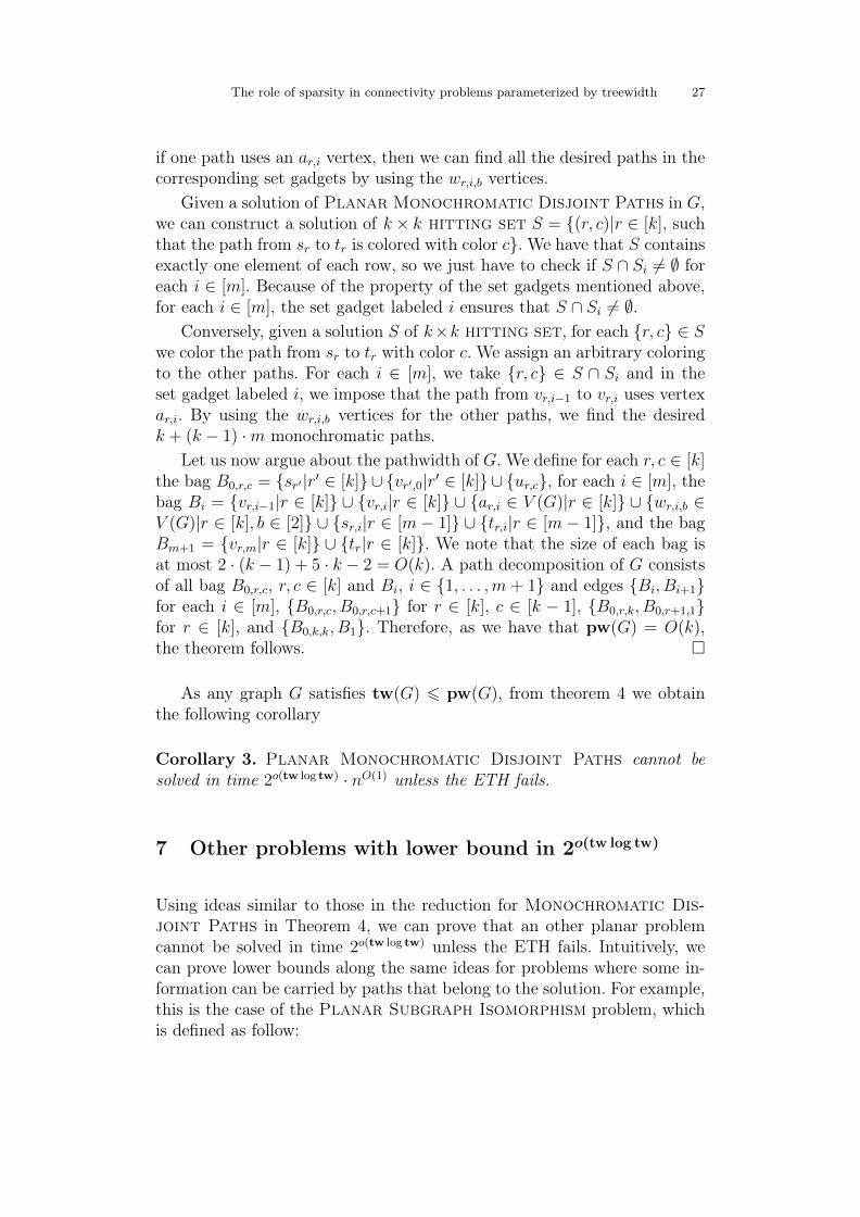
7 Other problems with lower bound in 2o(tw log tw)

Using ideas similar to those in the reduction for Monochromatic Dis-joint Paths in Theorem 4, we can prove that an other planar problemcannot be solved in time 2o(tw log tw) unless the ETH fails. Intuitively, wecan prove lower bounds along the same ideas for problems where some in-formation can be carried by paths that belong to the solution. For example,this is the case of the Planar Subgraph Isomorphism problem, whichis defined as follow:


Grr Grr Grr Grr

Path with k + 1 edges Path with k + 1 edges

Repeat a total of m times

Fig. 15. Reqr with m+ 1 elements Grr.

u v

Grg

The gadget.

Grg

The request.

Fig. 16. Expel gadget.

sr vr,0

Grr Grr Grr Grr

Fig. 17. The color-selection gadget.

Planar Subgraph IsomorphismInput: Two planar graphs G and H.Parameter: tw = tw(G).Question: Does G contains a subgraph isomorphic to H?

Lemma 5. Planar Subgraph Isomorphism cannot be solved in time2o(tw log tw) · nO(1) unless ETH fails.

Proof: We reduce again from k×k hitting set. Let k be an integer withk > 3 and S1, S2, . . . , Sm ⊆ [k]× [k] such that each set contains at most oneelement from each row of [k] × [k]. We construct a graph G similar to theone for Monochromatic Disjoint Path. We construct in the same timethe graph H. In this section, we call each maximal connected subgraph ofH a request. So H will be the union of all the requests we made. We modifythe expel gadget, the color selection gadget, and the avoid path gadget.As in Monochromatic Disjoint Paths, we create a gadget for eachrow {r} × [k] and make a request, Reqr, depicted in Fig. 15, for each ofthese gadgets, that choose a path and simulates a color for each row. Weadd the set gadget that ensures that S ∩ Si 6= ∅ for each i ∈ {1 . . .m}.For each r ∈ [k], the Reqr simulates the path from sr to tr that appearsin Monochromatic Disjoint Paths. The way it is insert in the color-


v1,i−1

v1,i

v2,i−1

v2,i

vk,i−1

vk,i

Gr1 Gr1 Gr1 Gr1

Gr2 Gr2 Gr2 Gr2

Gr2 Gr2 Gr2 Gr2

Grk Grk Grk Grk

Gr1

Gr2

Grk

EE

EE

EE

Fig. 18. Set gadget with (1, 3) ∈ S1, (2, 2) ∈ S2, . . . , (k, 1) ∈ Sk.

selection gadget simulates the color of the path sr . . . tr and fix the pathsit can use in the set gadgets as in Monochromatic Disjoint Paths.

More precisely, we define k+1 graphs that do not appear anywhere elsein the graph. For it, we take a grid of size k+2 in which we remove a vertex.We name Gr1, Gr2, . . . , Grk and Grg these grids. Gri, i ∈ [k], identifies thesubgraph corresponding to the row i, while Grg identifies the expel gadgetrequests. We redefine the expel gadget as depicted in Fig. 16 and the color-selection gadget as depicted in Fig. 17. We also redefine the set gadget asdepicted in Fig. 18 similarly to Monochromatic Disjoint Paths butwith the new expel gadget and a way to simulate in Planar SubgraphIsomorphism the color we have in Monochromatic Disjoint Paths.

The final graph we construct has the same shape depicted in Fig. 14but with the new gadgets instead. We define the planar graph H to be theunion of the m · (k − 1) expel gadget requests shown in Fig. 16 and therequest Reqr for each r ∈ [k].


u

s

u′

u′′

t

Fig. 19. The double-expel gadget.

All we have to specify is that we can use the path in the set gadgetthat simulates the colored path that appear in the reduction of PlanarMonochromatic Disjoint Paths only if we choose the correspondingcolor in the color-selection gadget. This property is given by the fact thatwe look for a path where the identify grids are space by the same numberof node each time and so, the color selected in the color-selection gadget ismaintain in each set gadget.

If S is a solution of k × k hitting set, by starting to find the requestReqi that simulates the correct color we find a solution to Planar Sub-graph Isomorphism as we have found a solution of MonochromaticDisjoint Paths. For the same reason that appear in the proof of PlanarMonochromatic Disjoint Paths lower bound, a solution of PlanarSubgraph Isomorphism defines a solution S of k × k hitting set. �

8 A Lower bounds for Planar Disjoint Paths

In this section we prove that, assuming the ETH, the Planar DisjointPaths problem cannot be solved in time 2o(tw) · nO(1).

Theorem 5. Planar Disjoint paths cannot be solved in time 2o(√n) ·

nO(1) unless the ETH fails.

Proof:We strongly follow the proof of Theorem 3. We reduce from Planar3-Colorability where the input graph has maximum degree at most 5.Let G = (V,E) be a planar graph with maximum degree at most 5 whereV = {v1, . . . , vn}. We proceed to construct a planar graph H togetherwith a planar embedding. We construct the same graph as in the proof ofTheorem 3 but where the gadgets are appropriately modified. We reuse theexpel gadget depicted in Fig. 11 and for each expel gadget, we ask for a


ai

bi

ci

si,0

ti,0

Fig. 20. The SCi-gadget: To keep planarity, there is a path-crossing gadget in each edge inter-section.

path between s and t. We redefine the double-expel gadget as depicted inFig. 19 and for each double-expel gadget, we ask for a path between s andt. We reuse the path-crossing gadget depicted in Fig. 8 and only ask forthe paths contained in the expel gadgets. We can now redefine the SCi-gadget depicted in Fig. 20, where each edge intersection is replaced by apath-crossing gadget. For each SCi-gadget we ask for a path between si,0and ti,0. We also define the bifurcate gadget depicted in Fig. 21 and foreach bifurcate gadget, we ask for a path between si,k and ti,k for k ∈ [9].We finally define the edge gadget depicted in Fig. 22 and for each edgegadget, we ask for a path between si,j,k and ti,j,k for k ∈ [3]. We can easilycheck that these gadgets preserve the same properties as the correspondingones in the proof of Theorem 3. Moreover, it is easy to see that a pathcannot turn in a path-crossing gadget. This completes the construction ofthe planar graph H.

Given a solution of Planar Disjoint Path in H, for each i ∈ [n],the selection of a cycle in the SCi-gadget selects a color for vi, that canbe any color that is shared by all color outputs of vi, and the edge gad-gets ensure that two adjacent vertices are in two different color classes.So in this way we obtain a solution of Planar 3-colorability in G.Conversely, given a solution of Planar 3-colorability in G, it definesa color output for {ai, bi, ci} for i ∈ [n]. Therefore, we select in the SCi-gadget the path that uses the vertex in {ai, bi, ci} corresponding to thecolor of vi. In the bifurcate gadget, we choose the paths that use the ver-tices in {ai,1, bi,1, ci,1, ai,2, bi,2, ci,2} leading to two identical color outputsthat are exactly the color output of {ai, bi, ci}. This selection keeps theproperty that the color output of {ai, bi, vi} is contained in the color out-put of {ai,1, bi,1, ci,1} and in the color output of {ai,2, bi,2, ci,2}, and leavesfree as many vertices as possible for other cycles in other gadgets. Insideeach edge gadget representing {vi, vj} ∈ E, we select the paths that areallowed by the free vertices. We complete our path selection by selecting afree path in each expel gadget contained in the path-crossing gadget.


si,1

ti,1

ai

si,2

ti,2

bi

si,3

ti,3

ci

ai,1

si,4 ti,4

bi,1

si,5 ti,4

ci,1

si,6 ti,6

si,7

ti,7

ai,2

si,8

ti,8

bi,2

si,9

ti,9

ci,2

Fig. 21. Bifurcate gadget: To keep planarity, there is a path-crossing gadget in each edge in-tersection.

As the degree of each vertex in G is bounded by 5, the number ofgadgets we introduce for each vi ∈ V (G) to construct H is also boundedby a constant, so the total number of vertices of H is linear in the number


si,j,1

ai,k

ti,j,1

aj,k

si,j,2

bi,k

ti,j,2

bj,k′

si,j,3

ci,k

ti,j,3

cj,k′

Fig. 22. Edge gadget: To keep planarity, there is a path-crossing gadget in each edge intersec-tion.

of vertices of G. Therefore if we could solve Planar Disjoint Paths intime 2o(

√n) · nO(1), then we could also solve Planar 3-Colorability in

time 2o(√n) · nO(1), which is impossible by Theorem 1 unless the ETH fails.

The theorem follows. �

From Theorem 8, we obtain the following corollary.

Corollary 4. The Planar Disjoint Paths problem cannot be solved intime 2o(tw) · nO(1) unless the ETH fails.

9 Further research

In this report, we show that planarity plays a role in time complexity forconnectivity problems parametrized by treewidth. But it is just the first stepand many problems are still open. In particular, we display few interestingproblems that we are still not able to solve:

– The Disjoint Path problem is known to be solvable in time 2O(tw log tw)·nO(1) in general graph [23] and we have not got better algorithm whenwe restrict the input graph to be planar. The best lower bound we


find for Planar Disjoint Path say that it cannot be solved in time2o(tw) · nO(1) unless ETH fails. We are still not able to define if it is aproblem of Type 2 or of Type 3 or even an intermediate type and thequestion is still open.

– The Subgraph Isomorphism problem is know to be solvable in time2O(h) ·nO(1) on planar graphs [6] and graphs on surfaces [2], where h is thenumber of vertices of a pattern graphH to be found in a host graph G onn vertices. As the Subgraph Isomorphism problem can be expressedin monadic second order logic then an algorithm that compute in timef(tw) · n exist. To our best knowledge no such algorithm is known, butwe prove that we cannot solve the problem in time 2o(tw log tw) · nO(1).

– Lokshtanov et al. [16] have proved that for a number of problems suchas Dominating Set or q-Coloring, the best known constant c inalgorithms of the form ctw · nO(1) on general graphs is the best possibleunless the Strong ETH fails. Is it possible to provide better constantsfor these problems on planar graphs? The existence of such algorithmswould permit to further refine the problems belonging to Type 1.

– Does a problem that can be solved in time 2o(tw) exist?– Finally, it would be interesting to obtain similar results for problems pa-

rameterized by pathwidth, and to extend our algorithms to more generalclasses of sparse graphs.

References

1. H. L. Bodlaender, M. Cygan, S. Kratsch, and J. Nederlof. Solving weighted and countingvariants of connectivity problems parameterized by treewidth deterministically in singleexponential time. CoRR, abs/1211.1505, 2012.

2. P. Bonsma. Surface split decompositions and subgraph isomorphism in graphs on surfaces.In Proc. of the 29th International Symposium on Theoretical Aspects of Computer Science(STACS), volume 14 of LIPIcs, pages 531–542, 2012.

3. B. Courcelle. The monadic second-order logic of graphs. I. Recognizable sets of finitegraphs. Information and Computation, 85(1):12–75, 1990.

4. M. Cygan, J. Nederlof, M. Pilipczuk, M. Pilipczuk, J. M. M. van Rooij, and J. O. Woj-taszczyk. Solving Connectivity Problems Parameterized by Treewidth in Single ExponentialTime. In Proc. of the 52nd Annual IEEE Symposium on Foundations of Computer Science(FOCS), pages 150–159. IEEE Computer Society, 2011.

5. R. Diestel. Graph Theory. Springer-Verlag, 3rd edition, 2005.6. F. Dorn. Planar subgraph isomorphism revisited. In Proc. of the 27th International Sym-

posium on Theoretical Aspects of Computer Science (STACS), volume 5 of LIPIcs, pages263–274, 2010.

7. F. Dorn, F. V. Fomin, and D. M. Thilikos. Fast Subexponential Algorithm for Non-localProblems on Graphs of Bounded Genus. In Proc. of the 10th Scandinavian Workshop onAlgorithm Theory (SWAT), volume 4059 of LNCS, pages 172–183, 2006.

8. F. Dorn, F. V. Fomin, and D. M. Thilikos. Catalan Structures and Dynamic Programmingin H-minor-free Graphs. In Proc. of the 19th annual ACM-SIAM Symposium on Discretealgorithms (SODA), pages 631–640, 2008.

9. F. Dorn, F. V. Fomin, and D. M. Thilikos. Catalan Structures and Dynamic Programmingin H-minor-free graphs. Journal of Computer and System Sciences, 78(5):1606–1622, 2012.


10. F. Dorn, E. Penninkx, H. L. Bodlaender, and F. V. Fomin. Efficient Exact Algorithms onPlanar Graphs: Exploiting Sphere Cut Decompositions. Algorithmica, 58(3):790–810, 2010.

11. J. Flum and M. Grohe. Parameterized Complexity Theory. Texts in Theoretical ComputerScience. Springer, 2006.

12. F. V. Fomin and D. M. Thilikos. New upper bounds on the decomposability of planargraphs. Journal of Graph Theory, 51(1):53–81, 2006.

13. M. Garey, D. Johnson, and R. E. Tarjan. The Planar Hamiltonian Circuit Problem isNP-Complete. In SIAM J Comput., pages 704–714, 1976.

14. R. Impagliazzo, R. Paturi, and F. Zane. Which Problems Have Strongly ExponentialComplexity? Journal of Computer and System Sciences, 63(4):512–530, 2001.

15. G. Kreweras. Sur les partitions non croisees d’un cycle. Discrete Mathematics, 1(4):333 –350, 1972.

16. D. Lokshtanov, D. Marx, and S. Saurabh. Known Algorithms on Graphs of BoundedTreewidth are Probably Optimal. In Proc. of the 22nd annual ACM-SIAM Symposium onDiscrete algorithms (SODA), pages 777–789, 2011.

17. D. Lokshtanov, D. Marx, and S. Saurabh. Slightly Superexponential Parameterized Prob-lems. In Proc. of the 22nd annual ACM-SIAM Symposium on Discrete algorithms (SODA),pages 760–776, 2011.

18. K. Mulmuley, U. V. Vazirani, and V. V. Vazirani. Matching is as easy as matrix inversion.In Proceedings of the nineteenth annual ACM symposium on Theory of computing, STOC’87, pages 345–354, New York, NY, USA, 1987. ACM.

19. N. Robertson and P. Seymour. Graph minors. ii. algorithmic aspects of tree-width. Journalof Algorithms, 7(3):309 – 322, 1986.

20. N. Robertson and P. Seymour. Graph minors. x. obstructions to tree-decomposition. Jour-nal of Combinatorial Theory, Series B, 52(2):153 – 190, 1991.

21. J. Rué, I. Sau, and D. M. Thilikos. Dynamic programming for graphs on surfaces. CoRR,abs/1104.2486, 2011, to appear in ACM Transactions on Algorithms (TALG). Short versionin the Proc. of ICALP’10.

22. J. Rué, I. Sau, and D. M. Thilikos. Dynamic Programming for H-minor-free Graphs.In Proc. of the 18th Annual International Conference on Computing and Combinatorics(COCOON), volume 7434 of LNCS, pages 86–97, 2012.

23. P. Scheffler. A practical linear time algorithm for disjoint paths in graphs with boundedtree-width. Fachbereich 3 Mathematik, Tech. Report 396/1994, FU Berlin, 1994.

The role of planarity in connectivity problems ... · The role of planarity in connectivity...

Documents

Transcript of The role of planarity in connectivity problems ... · The role of planarity in connectivity...