Monetary Law and Monetary Policy 4. Monetary policy – instruments and policies

NBP Working Paper No. 245
The role of bank balance sheets in monetary policy transmission. Evidence from PolandMariusz Kapuściński

Economic InstituteWarsaw, 2016
NBP Working Paper No. 245
The role of bank balance sheets in monetary policy transmission. Evidence from PolandMariusz Kapuściński

Published by: Narodowy Bank Polski Education & Publishing Department ul. Świętokrzyska 11/21 00-919 Warszawa, Poland phone +48 22 185 23 35 www.nbp.pl
ISSN 2084-624X
© Copyright Narodowy Bank Polski, 2016
Mariusz Kapuściński – Narodowy Bank Polski and Warsaw School of Economics; [email protected]
The views expressed in this paper are those of the author and do not necessarily represent those of Narodowy Bank Polski. I would like to thank Marta Korczak, Radosław Kotkowski, Tomasz Łyziak, Andrzej Sławiński, Dorota Ścibisz and Ewa Wróbel for useful comments. Any remaining errors are mine.

3NBP Working Paper No. 245
Contents1 Introduction 5
2 The bank lending channel of the monetary transmission mechanism – old and new 7
3 Empirical strategy 11
3.1 Models 113.2 Data 15
4 Results 17
4.1 Panel vector autoregressions 174.2 Univariate panel regressions 184.3 Counterfactual exercises 204.4 The traditional empirical strategy 21
5 Conclusion 24
Appendix 25

Narodowy Bank Polski4
Abstract
Abstract
This study investigates whether the effects of monetary policy are amplified
through its impact on bank balance sheet strength. Or, in other words, it tests
whether the bank lending channel of the monetary transmission mechanism (as
reformulated by Disyatat, 2011) works. To this end, panel vector autoregressions
with high frequency identification and univariate panel regressions are applied to
data for Poland. Counterfactual exercises show that the analysed channel accounts
for about 23% of a decrease in lending following a monetary policy impulse. This
is another piece of evidence showing that the financial accelerator works in both
non-financial and financial sector. In some cases it can make the interplay between
monetary and macroprudential policy non-trivial.
JEL classifications: E52, E51, C33, C23, E43
Keywords: monetary transmission mechanism, bank capital, panel vector autore-
gressions, high frequency identification
3
1 Introduction
Financial factors played the primary role in the Great Recession (2007-2009). The
turbulence started in August 2007 when BNP Paribas halted redemptions of three
investment funds. It intensified in September 2008 when Lehman Brothers filed for
bankruptcy. It is not surprising that since then financial markets in general, and banks
in particular, have been the subject of a larger share of economic studies. For example,
many of them attempt to analyse the macroeconomic role of banks within the dominant
dynamic stochastic general equilibrium framework in an increasingly useful for policy
analysis manner (for recent advances see, for example, Brzoza-Brzezina, 2014; Jakab
and Kumhof, 2015).
Besides observing more interest in banks, one can also find a changing approach
to them. Recently, a few papers pointed out that banks neither ‘multiply up’ central
bank money to create deposits nor do they intermediate loanable funds, as usually
assumed (McLeay et al., 2014; Werner, 2015; Jakab and Kumhof, 2015). Banks create
money making loans, with a central bank simply accommodating demand for reserves
(Goodhart, 2009). And in creating money banks are limited mainly by expected prof-
itability and capacity of their capital to absorb potential loan losses (fulfilling capital
requirements at the same time).1 It can make a difference for our understanding of
some economic phenomena and designing economic policy.
It also matters for understanding the role of banks and their balance sheets in
monetary policy transmission. There is a large body of literature on the bank lend-
ing channel, which started with a seminal paper of Bernanke and Blinder (1988) and
continues until today. In its traditional formulation, it argues that monetary tight-
ening reduces deposits and the ability of banks to make loans. As will be explained
later, taking into account the above-mentioned changes in the approach to banks, that
the traditional bank lending channel is operative seems unlikely. It has been already
pointed out by Disyatat (2011), who proposed an alternative formulation: a monetary
impulse can reduce loan supply through its impact on bank balance sheet strength.
It resembles bank balance sheet, bank capital and risk-pricing channels found earlier
(Chami and Cosimano, 2010; Van den Heuvel, 2006; Kishan and Opiela, 2012), with
some of them focusing on quantities and some on prices.
This study investigates whether such a mechanism works. It proposes an empirical
strategy to identify it, which is its main contribution to the literature. First, panel
vector autoregressions with high-frequency identification are applied to data for Poland
to check whether monetary policy matters for bank balance sheet strength (measured
by non-performing loans, profitability and a capital buffer). Second, the impact of bank
balance sheet strength on bank lending is analysed using univariate panel regressions.
1This is by no means a new finding. Werner (2014) argues that the ‘credit creation theory ofbanking’ was dominant in the first two decades of the 20th century.
4
5NBP Working Paper No. 245
Chapter 1
Abstract
This study investigates whether the effects of monetary policy are amplified
through its impact on bank balance sheet strength. Or, in other words, it tests
whether the bank lending channel of the monetary transmission mechanism (as
reformulated by Disyatat, 2011) works. To this end, panel vector autoregressions
with high frequency identification and univariate panel regressions are applied to
data for Poland. Counterfactual exercises show that the analysed channel accounts
for about 23% of a decrease in lending following a monetary policy impulse. This
is another piece of evidence showing that the financial accelerator works in both
non-financial and financial sector. In some cases it can make the interplay between
monetary and macroprudential policy non-trivial.
JEL classifications: E52, E51, C33, C23, E43
Keywords: monetary transmission mechanism, bank capital, panel vector autore-
gressions, high frequency identification
3
1 Introduction
Financial factors played the primary role in the Great Recession (2007-2009). The
turbulence started in August 2007 when BNP Paribas halted redemptions of three
investment funds. It intensified in September 2008 when Lehman Brothers filed for
bankruptcy. It is not surprising that since then financial markets in general, and banks
in particular, have been the subject of a larger share of economic studies. For example,
many of them attempt to analyse the macroeconomic role of banks within the dominant
dynamic stochastic general equilibrium framework in an increasingly useful for policy
analysis manner (for recent advances see, for example, Brzoza-Brzezina, 2014; Jakab
and Kumhof, 2015).
Besides observing more interest in banks, one can also find a changing approach
to them. Recently, a few papers pointed out that banks neither ‘multiply up’ central
bank money to create deposits nor do they intermediate loanable funds, as usually
assumed (McLeay et al., 2014; Werner, 2015; Jakab and Kumhof, 2015). Banks create
money making loans, with a central bank simply accommodating demand for reserves
(Goodhart, 2009). And in creating money banks are limited mainly by expected prof-
itability and capacity of their capital to absorb potential loan losses (fulfilling capital
requirements at the same time).1 It can make a difference for our understanding of
some economic phenomena and designing economic policy.
It also matters for understanding the role of banks and their balance sheets in
monetary policy transmission. There is a large body of literature on the bank lend-
ing channel, which started with a seminal paper of Bernanke and Blinder (1988) and
continues until today. In its traditional formulation, it argues that monetary tight-
ening reduces deposits and the ability of banks to make loans. As will be explained
later, taking into account the above-mentioned changes in the approach to banks, that
the traditional bank lending channel is operative seems unlikely. It has been already
pointed out by Disyatat (2011), who proposed an alternative formulation: a monetary
impulse can reduce loan supply through its impact on bank balance sheet strength.
It resembles bank balance sheet, bank capital and risk-pricing channels found earlier
(Chami and Cosimano, 2010; Van den Heuvel, 2006; Kishan and Opiela, 2012), with
some of them focusing on quantities and some on prices.
This study investigates whether such a mechanism works. It proposes an empirical
strategy to identify it, which is its main contribution to the literature. First, panel
vector autoregressions with high-frequency identification are applied to data for Poland
to check whether monetary policy matters for bank balance sheet strength (measured
by non-performing loans, profitability and a capital buffer). Second, the impact of bank
balance sheet strength on bank lending is analysed using univariate panel regressions.
1This is by no means a new finding. Werner (2014) argues that the ‘credit creation theory ofbanking’ was dominant in the first two decades of the 20th century.
4

Narodowy Bank Polski6
Finally, impulse response functions from the first step are compared with counterfactual
ones, which assume that the analysed channel does not work.
The results show that a monetary policy impulse increases non-performing loans,
and reduces bank profitability and a capital buffer. Weaker balance sheets, in turn, are
associated with lower lending growth. Overall, the bank lending channel (as reformu-
lated by Disyatat, 2011) accounts for about 23% of a decrease in lending following a
monetary policy impulse. This is another piece of evidence showing that the financial
accelerator works in both non-financial and financial sector. In some cases it can make
the interplay between monetary and macroprudential policy non-trivial.
For comparison, results from the traditional, less direct strategy for identifying the
bank lending channel are shown as well. It relies on comparing responses of different
groups of banks to monetary policy, assuming that some groups can better insulate
themselves from shocks. In this case it should be those with less non-performing loans,
more profitable and with a larger capital buffer. However, using this strategy would
not lead to the same conclusions. This is probably because it reveals nonlinearity in
responses due to many factors, including differences in portfolios of customers.
The paper is organised as follows. The second section provides a critical review
of the literature. The third one describes econometric models and data. The fourth
section shows results. The last one concludes.
5
2 The bank lending channel of the monetary transmission
mechanism – old and new
There is a large body of literature on the bank lending channel, which started with a
seminal paper of Bernanke and Blinder (1988). They modified the IS-LM model by
adding loans. Within such a framework monetary tightening works as follows. A central
bank conducts open market operations (reverse repo in this case) which drain reserves.
It is assumed that a reserve requirement is binding, so banks have to reduce deposits.
A lower amount of deposits, in turn, drives up interest rates. This is a so-called money
view on the transmission of monetary policy. Another one, an (‘old’) lending view,
argues that a decrease in deposits reduces loans, enhancing the first mechanism. It
does so because deposits are assumed to be funds that banks use to make loans.
Early discussions on this framework (see Kashyap and Stein, 1993 for a review)
pointed out that banks can replace deposits with other sources of funds, attenuating
the bank lending channel (Romer and Romer, 1990). However, as argued for example
by Stein (1998), for this channel to work it suffices that these other sources are more
costly. Another objection could be that nowadays reserve requirements are relatively
low, and that central banks signal their policy stance using a target for an interest rate
rather than open market operations. Furthermore, they simply accommodate demand
for reserves (Goodhart, 2009). Otherwise they would not achieve the interest rate
target (see Disyatat, 2008). But a decline in deposits could also take place due to
portfolio substitution following an interest rate increase, assuming that interest rate on
deposits does not change (or changes less than a bond yield). Therefore, some more
recent studies (for example, Ehrmann et al., 2001) abstract from reserves.
To test the bank lending channel most papers apply some form of an empirical
strategy proposed by Kashyap and Stein (1995). It relies on comparing responses of
different groups of banks to monetary policy, assuming that certain groups can better
insulate themselves from a decrease in deposits. In the above-mentioned study they
showed that in the United States loan portfolios of smaller banks decline more after
monetary tightening, as (according to their interpretation) they cannot easily raise non-
deposit sources of funds. Kashyap and Stein (2000) found that this stronger decline
holds especially for banks small and with less liquid assets. According to Kishan and
Opiela (2000) – for small and undercapitalised banks.2 For liquidity the exact inter-
pretation is usually different. It is argued that more liquid banks can compensate for
a decrease in deposits by selling securities. There is also an alternative explanation for
capitalisation. Peek and Rosengren (1995), and Kishan and Opiela (2006) showed that
banks respond to monetary policy differently depending on whether they are capital-
2On the other hand, more recently Carpenter and Demiralp (2012) showed that in the United Statesresponses of bank balance sheet variables, with banks divided by size, liquidity and capitalisation, areinconsistent with the bank lending channel being operative.
6
7NBP Working Paper No. 245
Chapter 2
Finally, impulse response functions from the first step are compared with counterfactual
ones, which assume that the analysed channel does not work.
The results show that a monetary policy impulse increases non-performing loans,
and reduces bank profitability and a capital buffer. Weaker balance sheets, in turn, are
associated with lower lending growth. Overall, the bank lending channel (as reformu-
lated by Disyatat, 2011) accounts for about 23% of a decrease in lending following a
monetary policy impulse. This is another piece of evidence showing that the financial
accelerator works in both non-financial and financial sector. In some cases it can make
the interplay between monetary and macroprudential policy non-trivial.
For comparison, results from the traditional, less direct strategy for identifying the
bank lending channel are shown as well. It relies on comparing responses of different
groups of banks to monetary policy, assuming that some groups can better insulate
themselves from shocks. In this case it should be those with less non-performing loans,
more profitable and with a larger capital buffer. However, using this strategy would
not lead to the same conclusions. This is probably because it reveals nonlinearity in
responses due to many factors, including differences in portfolios of customers.
The paper is organised as follows. The second section provides a critical review
of the literature. The third one describes econometric models and data. The fourth
section shows results. The last one concludes.
5
2 The bank lending channel of the monetary transmission
mechanism – old and new
There is a large body of literature on the bank lending channel, which started with a
seminal paper of Bernanke and Blinder (1988). They modified the IS-LM model by
adding loans. Within such a framework monetary tightening works as follows. A central
bank conducts open market operations (reverse repo in this case) which drain reserves.
It is assumed that a reserve requirement is binding, so banks have to reduce deposits.
A lower amount of deposits, in turn, drives up interest rates. This is a so-called money
view on the transmission of monetary policy. Another one, an (‘old’) lending view,
argues that a decrease in deposits reduces loans, enhancing the first mechanism. It
does so because deposits are assumed to be funds that banks use to make loans.
Early discussions on this framework (see Kashyap and Stein, 1993 for a review)
pointed out that banks can replace deposits with other sources of funds, attenuating
the bank lending channel (Romer and Romer, 1990). However, as argued for example
by Stein (1998), for this channel to work it suffices that these other sources are more
costly. Another objection could be that nowadays reserve requirements are relatively
low, and that central banks signal their policy stance using a target for an interest rate
rather than open market operations. Furthermore, they simply accommodate demand
for reserves (Goodhart, 2009). Otherwise they would not achieve the interest rate
target (see Disyatat, 2008). But a decline in deposits could also take place due to
portfolio substitution following an interest rate increase, assuming that interest rate on
deposits does not change (or changes less than a bond yield). Therefore, some more
recent studies (for example, Ehrmann et al., 2001) abstract from reserves.
To test the bank lending channel most papers apply some form of an empirical
strategy proposed by Kashyap and Stein (1995). It relies on comparing responses of
different groups of banks to monetary policy, assuming that certain groups can better
insulate themselves from a decrease in deposits. In the above-mentioned study they
showed that in the United States loan portfolios of smaller banks decline more after
monetary tightening, as (according to their interpretation) they cannot easily raise non-
deposit sources of funds. Kashyap and Stein (2000) found that this stronger decline
holds especially for banks small and with less liquid assets. According to Kishan and
Opiela (2000) – for small and undercapitalised banks.2 For liquidity the exact inter-
pretation is usually different. It is argued that more liquid banks can compensate for
a decrease in deposits by selling securities. There is also an alternative explanation for
capitalisation. Peek and Rosengren (1995), and Kishan and Opiela (2006) showed that
banks respond to monetary policy differently depending on whether they are capital-
2On the other hand, more recently Carpenter and Demiralp (2012) showed that in the United Statesresponses of bank balance sheet variables, with banks divided by size, liquidity and capitalisation, areinconsistent with the bank lending channel being operative.
6

Narodowy Bank Polski8
constrained or not. If they are, their ability to expand lending following easing of
monetary policy is limited, irrespective of whether other constraints are binding. But
overall, significant differences in responses with the ‘correct’ sign are interpreted as an
indication that the bank lending channel works.
The literature expanded in two directions. First, size, liquidity and capitalisation
were supplemented with other characteristics. Gambacorta (2005), and Cetorelli and
Goldberg (2008) found that access to funding within holdings and global banks can
insulate from monetary impulses. According to Altunbas et al. (2009) the same holds
for using securitisation, which makes assets effectively more liquid. Altunbas et al.
(2010) showed that bank risk can be considered as another proxy for access to non-
deposit sources of funds.
Second, similar exercises were conducted for other countries/regions. For example,
for Europe Ehrmann et al. (2001) showed that in some countries banks respond to mon-
etary policy differently, depending on liquidity of their assets. Altunbas et al. (2002)
found nonlinear responses with respect to capitalisation. Specifically, according to
these studies loan portfolios of less liquid/undercapitalised banks decrease more follow-
ing monetary tightening. There are also a few papers for Poland, with mixed results.
Pawłowska and Wróbel (2002) showed that size, liquidity and capitalisation matter
when it comes to responses of bank loans to monetary policy, but surprisingly more
liquid banks respond more strongly. The latter result can also be found in Chmielewski
(2005), who additionally established that there is a role for bank risk and ownership
(with more risky and foreign banks reducing lending more). Havrylchyk and Jurzyk
(2005) confirmed his finding on ownership, but also showed that the role of size, if
any, can go in the opposite direction than in Pawłowska and Wróbel (2002). Matousek
and Sarantis (2009) arrived at the same conclusion on size. On the other hand, they
confirmed the result of Pawłowska and Wróbel (2002) on capital. According to Opiela
(2008) banks with a full deposit guarantee used to contract lending more than those
with a partial guarantee after monetary tightening. However, this is no longer relevant,
as currently deposits in all banks are guaranteed in the same way. For a more extensive
survey on this literature see Peek and Rosengren (2013).
But Disyatat (2011) raised more fundamental objections to the traditional approach
to the bank lending channel. To begin with, it was already mentioned that monetary
tightening/easing can be implemented without any additional open market operation.
For example, currently Narodowy Bank Polski (NBP) makes an interest rate decision
11 times a year on first or second Wednesday of a given month. Regular open market
operations are conducted each Friday. Say, a 25 basis point increase in a reference rate
(which is a yield on 1-week operations absorbing liquidity) on Wednesday influences
interbank interest rates immediately (if expected even in advance), not on next Friday.3
In addition, a volume of open market operations is unlikely to be affected by the interest
3Of course, it also holds for central banks in developed economies (see Borio, 1997).
7
rate decision, as demand for reserves is largely interest-inelastic. Surplus liquidity has
to be absorbed/missing liquidity has to be provided simply to achieve the interest rate
target. And a given level of reserves can coexist with many different levels of interest
rates (this is a so-called decoupling principle, see Borio and Disyatat, 2010). Therefore,
a link: reserves-money multiplier-deposits rather cannot be a starting point for the bank
lending channel.
Another one could be a decrease in deposits due to portfolio substitution. But
do aggregate deposits decline following an interest rate increase? And if they do, for
what reason? The key assumption is that interest rate on deposits does not change
(or changes less than a bond yield) after monetary tightening. Indeed, in the United
States there used to be Requlation Q, which imposed ceilings on saving deposit rates.
But it was phased out in 1986. Currently there is practically no opportunity cost in
holding saving deposits, or at least a bond yield does not constitute such a cost (Stiglitz
and Greenwald, 2003). On the other hand, demand deposits usually offer lower or no
return. But these are kept rather for other (transactional) purposes and should not be
interest-elastic in the first place. Furthermore, although deposits are being transferred
between banks on a large scale every day, an aggregate decline in them can happen only
in specific circumstances. There are three most important cases. First, when deposits
are exchanged for cash. Second, when non-banks buy financial assets from banks. It
should be noted that when a household buys a bond from a non-bank corporation it
exchanges a deposit for a bond. Now it is the corporation who has the deposit in a
bank, not the household. However, an aggregate amount of deposits does not change.
But when the household buys this bond from the bank deposit of the household is
‘destroyed’. The same happens when non-banks repay loans to banks, which is the
third case of interest (see McLeay et al., 2014). In other words, when loans decrease so
do deposits, not the other way around.
The last point leads to another one, probably the most important in this discussion.
Namely, banks do not intermediate deposits, they create deposits making loans (see
Jakab and Kumhof, 2015). Put differently, new loans are not funded by recycling of
deposits that were made earlier, but by creation of new deposits. This is what differ-
entiates banks from other corporations, including non-bank corporations specialised in
making payday loans. And in creating money banks are limited mainly by expected
profitability and capacity of their capital to absorb potential loan losses (fulfilling cap-
ital requirements at the same time). Of course, a given bank has to roughly balance
deposit outflows with inflows, as the balancing item for a change in deposits is a change
in reserves. If the bank does not have sufficient reserves to settle the net outflow, it has
to borrow them. This can turn out to be unsustainable in the long run (see the case
of Northern Rock during the last crisis, Shin, 2009). But this is a different point than
saying that banks are limited in their lending activity by deposits. Taking all this into
account, that the traditional bank lending channel is operative seems unlikely.
8

9NBP Working Paper No. 245
The bank lending channel of the monetary transmission mechanism – old and new
constrained or not. If they are, their ability to expand lending following easing of
monetary policy is limited, irrespective of whether other constraints are binding. But
overall, significant differences in responses with the ‘correct’ sign are interpreted as an
indication that the bank lending channel works.
The literature expanded in two directions. First, size, liquidity and capitalisation
were supplemented with other characteristics. Gambacorta (2005), and Cetorelli and
Goldberg (2008) found that access to funding within holdings and global banks can
insulate from monetary impulses. According to Altunbas et al. (2009) the same holds
for using securitisation, which makes assets effectively more liquid. Altunbas et al.
(2010) showed that bank risk can be considered as another proxy for access to non-
deposit sources of funds.
Second, similar exercises were conducted for other countries/regions. For example,
for Europe Ehrmann et al. (2001) showed that in some countries banks respond to mon-
etary policy differently, depending on liquidity of their assets. Altunbas et al. (2002)
found nonlinear responses with respect to capitalisation. Specifically, according to
these studies loan portfolios of less liquid/undercapitalised banks decrease more follow-
ing monetary tightening. There are also a few papers for Poland, with mixed results.
Pawłowska and Wróbel (2002) showed that size, liquidity and capitalisation matter
when it comes to responses of bank loans to monetary policy, but surprisingly more
liquid banks respond more strongly. The latter result can also be found in Chmielewski
(2005), who additionally established that there is a role for bank risk and ownership
(with more risky and foreign banks reducing lending more). Havrylchyk and Jurzyk
(2005) confirmed his finding on ownership, but also showed that the role of size, if
any, can go in the opposite direction than in Pawłowska and Wróbel (2002). Matousek
and Sarantis (2009) arrived at the same conclusion on size. On the other hand, they
confirmed the result of Pawłowska and Wróbel (2002) on capital. According to Opiela
(2008) banks with a full deposit guarantee used to contract lending more than those
with a partial guarantee after monetary tightening. However, this is no longer relevant,
as currently deposits in all banks are guaranteed in the same way. For a more extensive
survey on this literature see Peek and Rosengren (2013).
But Disyatat (2011) raised more fundamental objections to the traditional approach
to the bank lending channel. To begin with, it was already mentioned that monetary
tightening/easing can be implemented without any additional open market operation.
For example, currently Narodowy Bank Polski (NBP) makes an interest rate decision
11 times a year on first or second Wednesday of a given month. Regular open market
operations are conducted each Friday. Say, a 25 basis point increase in a reference rate
(which is a yield on 1-week operations absorbing liquidity) on Wednesday influences
interbank interest rates immediately (if expected even in advance), not on next Friday.3
In addition, a volume of open market operations is unlikely to be affected by the interest
3Of course, it also holds for central banks in developed economies (see Borio, 1997).
7
rate decision, as demand for reserves is largely interest-inelastic. Surplus liquidity has
to be absorbed/missing liquidity has to be provided simply to achieve the interest rate
target. And a given level of reserves can coexist with many different levels of interest
rates (this is a so-called decoupling principle, see Borio and Disyatat, 2010). Therefore,
a link: reserves-money multiplier-deposits rather cannot be a starting point for the bank
lending channel.
Another one could be a decrease in deposits due to portfolio substitution. But
do aggregate deposits decline following an interest rate increase? And if they do, for
what reason? The key assumption is that interest rate on deposits does not change
(or changes less than a bond yield) after monetary tightening. Indeed, in the United
States there used to be Requlation Q, which imposed ceilings on saving deposit rates.
But it was phased out in 1986. Currently there is practically no opportunity cost in
holding saving deposits, or at least a bond yield does not constitute such a cost (Stiglitz
and Greenwald, 2003). On the other hand, demand deposits usually offer lower or no
return. But these are kept rather for other (transactional) purposes and should not be
interest-elastic in the first place. Furthermore, although deposits are being transferred
between banks on a large scale every day, an aggregate decline in them can happen only
in specific circumstances. There are three most important cases. First, when deposits
are exchanged for cash. Second, when non-banks buy financial assets from banks. It
should be noted that when a household buys a bond from a non-bank corporation it
exchanges a deposit for a bond. Now it is the corporation who has the deposit in a
bank, not the household. However, an aggregate amount of deposits does not change.
But when the household buys this bond from the bank deposit of the household is
‘destroyed’. The same happens when non-banks repay loans to banks, which is the
third case of interest (see McLeay et al., 2014). In other words, when loans decrease so
do deposits, not the other way around.
The last point leads to another one, probably the most important in this discussion.
Namely, banks do not intermediate deposits, they create deposits making loans (see
Jakab and Kumhof, 2015). Put differently, new loans are not funded by recycling of
deposits that were made earlier, but by creation of new deposits. This is what differ-
entiates banks from other corporations, including non-bank corporations specialised in
making payday loans. And in creating money banks are limited mainly by expected
profitability and capacity of their capital to absorb potential loan losses (fulfilling cap-
ital requirements at the same time). Of course, a given bank has to roughly balance
deposit outflows with inflows, as the balancing item for a change in deposits is a change
in reserves. If the bank does not have sufficient reserves to settle the net outflow, it has
to borrow them. This can turn out to be unsustainable in the long run (see the case
of Northern Rock during the last crisis, Shin, 2009). But this is a different point than
saying that banks are limited in their lending activity by deposits. Taking all this into
account, that the traditional bank lending channel is operative seems unlikely.
8

Narodowy Bank Polski10
Therefore, Disyatat (2011) proposed an alternative (‘new’) formulation for the bank
lending channel. He argued that the effects of monetary policy can be amplified through
its impact on bank balance sheet strength, which influences loan supply. The exact
mechanism is supposed to work as follows. Monetary tightening, implemented by an
interest rate increase, affects bank cash flows, net interest margins, asset valuation and
asset quality. This is reflected in lower profits and capital.4 Weaker bank balance
sheets, in turn, lead to higher costs of funds for both banks and their customers, which
reduces lending.
This description resembles a few mechanisms found earlier: bank balance sheet,
bank capital and risk-pricing channels (Chami and Cosimano, 2010; Van den Heuvel,
2006; Kishan and Opiela, 2012).5 The first two are focused on quantities and the third
one on prices. All of them are similar to the balance sheet channel/financial accelerator
(Bernanke et al., 1999) but on a bank level instead of a level of non-financial corpor-
ations. Indeed, for parsimony it would be probably best to refer to a single balance
sheet channel, operating for non-bank corporations, banks, as well as households.6 This
is what, for example, Igan et al. (2013) implicitly do in their empirical study on the
relationship between monetary policy and balance sheets in general. That monetary
policy works through its impact on the health of banks is also basis for a so-called I
theory of money (Brunnermeier and Sannikov, 2016).
Importantly, the results from the literature on the traditional bank lending channel
can be to a large extent reconciled with its revised version (Disyatat, 2011). For
example, smaller, less liquid and undercapitalised banks can be perceived as more
risky and therefore face a stronger increase in their cost of funding following monetary
tightening. It should be noted that what matters is existing, not necessarily new
funding. And that larger reliance on market-based funding amplifies, not attenuates the
mechanism. This is an important difference in implications between the two approaches
to the bank lending channel.
Even if the traditional empirical strategy can give some indication whether the
effects of monetary policy are amplified through its impact on bank balance sheet
strength, Disyatat (2011) suggests to use strategies based on interest rates or spreads,
rather than quantities. Besides the above-mentioned studies on the risk-pricing channel,
this is what, for example, Gambacorta (2008) and de Haan et al. (2015) do. But since
usually micro data on interest rates is scarce, and because quantity rationing seems
to be both theoretically (see Jakab and Kumhof, 2015) and empirically (see Bassett
et al., 2014; Altavilla et al., 2015) important, one can also directly investigate whether
monetary policy indeed affects bank balance sheet strength and, if it does, whether it
4On the role of bank capital see Holmstrom and Tirole (1997), and Borio and Zhu (2012).5On the bank balance sheet channel see also Hosono and Miyakawa (2014), on the bank capital
channel Meh (2011), on the risk-pricing channel Breitenlechner and Scharler (2015).6The point that the balance sheet channel can work for both non-bank corporations and banks can
be found already in Bernanke and Gertler (1995), as well as in Bernanke (2007).
9
matters for bank lending. This study proposes to use such an empirical strategy.
10
3 Empirical strategy
3.1 Models
The empirical investigation is conducted in three steps. The first one checks whether
monetary policy matters for bank balance sheet strength. To this end, there are estim-
ated panel vector autoregressions in the following form:7
yit “ A0i ` A1yit´1 ` A2yit´2 ` ¨ ¨ ¨ ` Apyit´p ` Bxit ` eit, (1)
where i and t are unit and time subscripts, p is a number of lags, yit is a vector of
endogenous variables, xit is a vector of exogenous variables (possibly in lags), eit is a
vector of error terms, A0i is a vector of fixed effects (intercept terms), and A1, A2, . . . , Ap
and B are matrices of other parameters. These models allow to capture dynamic
interrelations between variables, which are especially important in this case. Error
terms are assumed to be identically and independently distributed, with a covariance
matrix Σ.
In line with the empirical literature on the bank lending channel units are assumed
to be heterogeneous only in intercept terms. This is reflected in a i subscript for a
vector A0. In static panel data models fixed effects are usually eliminated by a within
transformation – subtraction of a unit-specific average of a given variable from each
observation. Then, estimation is conducted on transformed variables using simple
ordinary least squares (OLS). However, such a transformation causes bias in estimates
when a lagged dependent variable is used as a regressor (in panel vector autoregressions
it is, in each equation). This is because a within transformed lagged dependent variable
is correlated with a within transformed error.
The most common way to avoid this problem is to remove fixed effects by a first
difference transformation. In such a case, parameters are estimated using instru-
mental variables (IV) or generalised method of moments (GMM), with first differenced
variables instrumented by their lagged levels or first differences. These are so-called
Anderson-Hsiao and Arellano-Bond/Blundell-Bond estimators. The problem is that
the first one is inefficient and that the Sargan test for overidentifying restrictions for
the second one is uninformative for models with the number of units smaller that the
number of instruments (that would be the case in this study, even using the most parsi-
monious specification). Moreover, first differences for some variables seem unnatural.
Taking this considerations into account, another transformation is used. Namely, fixed
effects are removed calculating forward orthogonal deviations, which are differences
between each observation and a unit-specific average of future observations of a given
variable. Parameters are estimated using GMM, instrumenting transformed variables
7Estimation is conducted using a pvar package in Stata (Abrigo and Love, 2015).
11
with untransformed ones.
In order to quantify the effects of monetary policy in panel vector autoregressions
(and in non-structural models in general), endogenous and exogenous policy actions
have to be separated from each other. Or, in other words, monetary policy shocks
have to be identified. Here, this is achieved using (relatively) high-frequency data from
financial markets. Specifically, a ‘current interest rate change’ factor from Kapuściński
(2015), reflecting exogenous policy actions, is employed as one of variables. It was
obtained following a method of Gurkaynak et al. (2005). First, there were calculated
changes in variables representing the expected path of interest rates one year ahead,
within two-day windows around policy meetings. Second, they were ‘compressed’ using
principal components. Third, the first two factors were rotated and normalised, so that
one of them could be interpreted as an unexpected component of changes in the current
interest rate and the other one as a proxy for central bank communication. The first
one is used here. For details see Kapuściński (2015).
Monetary policy shocks identified with high-frequency data have been used in vector
autoregressions since Bagliano and Favero (1999). They employed them as an exogen-
ous variable and calculated dynamic multipliers (instead of impulse response functions,
as usually in vector autoregressions) in order to analyse the effects of monetary policy,
using an interest rate as one of endogenous variables at the same time. More recently,
Barakchian and Crowe (2013) used them as an endogenous variable instead of an in-
terest rate. Gertler and Karadi (2015), and Passari and Rey (2015) instrumented an
interest rate with these shocks.
High-frequency identification was chosen because it has the potential to correct for
some drawbacks of more traditional identification strategies, such as short-run restric-
tions. These include a time-invariant structure (parameters in a monetary policy rule
can change over time), a restricted information set (policymakers can track literally
hundreds of variables), the use of final, revised data (estimates of GDP frequently
change) and long distributed lags (there is little reason to believe that policymakers
respond to, for example, inflation or GDP from a year earlier, Rudebusch, 1998).
The baseline model includes the economic sentiment indicator (ESI), a monetary
policy shock, non-performing loan (NPL) ratio, a return on assets (ROA)8, a capital
buffer and loans as endogenous variables (with such an ordering in Cholesky decom-
position), as well as seasonal dummies as exogenous variables. The choice of the ESI
instead of GDP is motivated by an inherent simultaneity between GDP and loans,
which makes the choice of Cholesky ordering non-trivial. On the one hand, for ex-
ample, when a corporation wants to make an investment and finance it with a loan, it
is investment demand what drives loans. But on the other hand, it is acceptance of
the loan what makes the investment possible. Moreover, the change in loans funds the
level of loan-financed expenditures (Biggs et al., 2009), while it seems more natural to
8The use of a return on equity does not change the results.
12

11NBP Working Paper No. 245
Chapter 3
Therefore, Disyatat (2011) proposed an alternative (‘new’) formulation for the bank
lending channel. He argued that the effects of monetary policy can be amplified through
its impact on bank balance sheet strength, which influences loan supply. The exact
mechanism is supposed to work as follows. Monetary tightening, implemented by an
interest rate increase, affects bank cash flows, net interest margins, asset valuation and
asset quality. This is reflected in lower profits and capital.4 Weaker bank balance
sheets, in turn, lead to higher costs of funds for both banks and their customers, which
reduces lending.
This description resembles a few mechanisms found earlier: bank balance sheet,
bank capital and risk-pricing channels (Chami and Cosimano, 2010; Van den Heuvel,
2006; Kishan and Opiela, 2012).5 The first two are focused on quantities and the third
one on prices. All of them are similar to the balance sheet channel/financial accelerator
(Bernanke et al., 1999) but on a bank level instead of a level of non-financial corpor-
ations. Indeed, for parsimony it would be probably best to refer to a single balance
sheet channel, operating for non-bank corporations, banks, as well as households.6 This
is what, for example, Igan et al. (2013) implicitly do in their empirical study on the
relationship between monetary policy and balance sheets in general. That monetary
policy works through its impact on the health of banks is also basis for a so-called I
theory of money (Brunnermeier and Sannikov, 2016).
Importantly, the results from the literature on the traditional bank lending channel
can be to a large extent reconciled with its revised version (Disyatat, 2011). For
example, smaller, less liquid and undercapitalised banks can be perceived as more
risky and therefore face a stronger increase in their cost of funding following monetary
tightening. It should be noted that what matters is existing, not necessarily new
funding. And that larger reliance on market-based funding amplifies, not attenuates the
mechanism. This is an important difference in implications between the two approaches
to the bank lending channel.
Even if the traditional empirical strategy can give some indication whether the
effects of monetary policy are amplified through its impact on bank balance sheet
strength, Disyatat (2011) suggests to use strategies based on interest rates or spreads,
rather than quantities. Besides the above-mentioned studies on the risk-pricing channel,
this is what, for example, Gambacorta (2008) and de Haan et al. (2015) do. But since
usually micro data on interest rates is scarce, and because quantity rationing seems
to be both theoretically (see Jakab and Kumhof, 2015) and empirically (see Bassett
et al., 2014; Altavilla et al., 2015) important, one can also directly investigate whether
monetary policy indeed affects bank balance sheet strength and, if it does, whether it
4On the role of bank capital see Holmstrom and Tirole (1997), and Borio and Zhu (2012).5On the bank balance sheet channel see also Hosono and Miyakawa (2014), on the bank capital
channel Meh (2011), on the risk-pricing channel Breitenlechner and Scharler (2015).6The point that the balance sheet channel can work for both non-bank corporations and banks can
be found already in Bernanke and Gertler (1995), as well as in Bernanke (2007).
9
matters for bank lending. This study proposes to use such an empirical strategy.
10
3 Empirical strategy
3.1 Models
The empirical investigation is conducted in three steps. The first one checks whether
monetary policy matters for bank balance sheet strength. To this end, there are estim-
ated panel vector autoregressions in the following form:7
yit “ A0i ` A1yit´1 ` A2yit´2 ` ¨ ¨ ¨ ` Apyit´p ` Bxit ` eit, (1)
where i and t are unit and time subscripts, p is a number of lags, yit is a vector of
endogenous variables, xit is a vector of exogenous variables (possibly in lags), eit is a
vector of error terms, A0i is a vector of fixed effects (intercept terms), and A1, A2, . . . , Ap
and B are matrices of other parameters. These models allow to capture dynamic
interrelations between variables, which are especially important in this case. Error
terms are assumed to be identically and independently distributed, with a covariance
matrix Σ.
In line with the empirical literature on the bank lending channel units are assumed
to be heterogeneous only in intercept terms. This is reflected in a i subscript for a
vector A0. In static panel data models fixed effects are usually eliminated by a within
transformation – subtraction of a unit-specific average of a given variable from each
observation. Then, estimation is conducted on transformed variables using simple
ordinary least squares (OLS). However, such a transformation causes bias in estimates
when a lagged dependent variable is used as a regressor (in panel vector autoregressions
it is, in each equation). This is because a within transformed lagged dependent variable
is correlated with a within transformed error.
The most common way to avoid this problem is to remove fixed effects by a first
difference transformation. In such a case, parameters are estimated using instru-
mental variables (IV) or generalised method of moments (GMM), with first differenced
variables instrumented by their lagged levels or first differences. These are so-called
Anderson-Hsiao and Arellano-Bond/Blundell-Bond estimators. The problem is that
the first one is inefficient and that the Sargan test for overidentifying restrictions for
the second one is uninformative for models with the number of units smaller that the
number of instruments (that would be the case in this study, even using the most parsi-
monious specification). Moreover, first differences for some variables seem unnatural.
Taking this considerations into account, another transformation is used. Namely, fixed
effects are removed calculating forward orthogonal deviations, which are differences
between each observation and a unit-specific average of future observations of a given
variable. Parameters are estimated using GMM, instrumenting transformed variables
7Estimation is conducted using a pvar package in Stata (Abrigo and Love, 2015).
11
3 Empirical strategy
3.1 Models
The empirical investigation is conducted in three steps. The first one checks whether
monetary policy matters for bank balance sheet strength. To this end, there are estim-
ated panel vector autoregressions in the following form:7
yit “ A0i ` A1yit´1 ` A2yit´2 ` ¨ ¨ ¨ ` Apyit´p ` Bxit ` eit, (1)
where i and t are unit and time subscripts, p is a number of lags, yit is a vector of
endogenous variables, xit is a vector of exogenous variables (possibly in lags), eit is a
vector of error terms, A0i is a vector of fixed effects (intercept terms), and A1, A2, . . . , Ap
and B are matrices of other parameters. These models allow to capture dynamic
interrelations between variables, which are especially important in this case. Error
terms are assumed to be identically and independently distributed, with a covariance
matrix Σ.
In line with the empirical literature on the bank lending channel units are assumed
to be heterogeneous only in intercept terms. This is reflected in a i subscript for a
vector A0. In static panel data models fixed effects are usually eliminated by a within
transformation – subtraction of a unit-specific average of a given variable from each
observation. Then, estimation is conducted on transformed variables using simple
ordinary least squares (OLS). However, such a transformation causes bias in estimates
when a lagged dependent variable is used as a regressor (in panel vector autoregressions
it is, in each equation). This is because a within transformed lagged dependent variable
is correlated with a within transformed error.
The most common way to avoid this problem is to remove fixed effects by a first
difference transformation. In such a case, parameters are estimated using instru-
mental variables (IV) or generalised method of moments (GMM), with first differenced
variables instrumented by their lagged levels or first differences. These are so-called
Anderson-Hsiao and Arellano-Bond/Blundell-Bond estimators. The problem is that
the first one is inefficient and that the Sargan test for overidentifying restrictions for
the second one is uninformative for models with the number of units smaller that the
number of instruments (that would be the case in this study, even using the most parsi-
monious specification). Moreover, first differences for some variables seem unnatural.
Taking this considerations into account, another transformation is used. Namely, fixed
effects are removed calculating forward orthogonal deviations, which are differences
between each observation and a unit-specific average of future observations of a given
variable. Parameters are estimated using GMM, instrumenting transformed variables
7Estimation is conducted using a pvar package in Stata (Abrigo and Love, 2015).
11
with untransformed ones.
In order to quantify the effects of monetary policy in panel vector autoregressions
(and in non-structural models in general), endogenous and exogenous policy actions
have to be separated from each other. Or, in other words, monetary policy shocks
have to be identified. Here, this is achieved using (relatively) high-frequency data from
financial markets. Specifically, a ‘current interest rate change’ factor from Kapuściński
(2015), reflecting exogenous policy actions, is employed as one of variables. It was
obtained following a method of Gurkaynak et al. (2005). First, there were calculated
changes in variables representing the expected path of interest rates one year ahead,
within two-day windows around policy meetings. Second, they were ‘compressed’ using
principal components. Third, the first two factors were rotated and normalised, so that
one of them could be interpreted as an unexpected component of changes in the current
interest rate and the other one as a proxy for central bank communication. The first
one is used here. For details see Kapuściński (2015).
Monetary policy shocks identified with high-frequency data have been used in vector
autoregressions since Bagliano and Favero (1999). They employed them as an exogen-
ous variable and calculated dynamic multipliers (instead of impulse response functions,
as usually in vector autoregressions) in order to analyse the effects of monetary policy,
using an interest rate as one of endogenous variables at the same time. More recently,
Barakchian and Crowe (2013) used them as an endogenous variable instead of an in-
terest rate. Gertler and Karadi (2015), and Passari and Rey (2015) instrumented an
interest rate with these shocks.
High-frequency identification was chosen because it has the potential to correct for
some drawbacks of more traditional identification strategies, such as short-run restric-
tions. These include a time-invariant structure (parameters in a monetary policy rule
can change over time), a restricted information set (policymakers can track literally
hundreds of variables), the use of final, revised data (estimates of GDP frequently
change) and long distributed lags (there is little reason to believe that policymakers
respond to, for example, inflation or GDP from a year earlier, Rudebusch, 1998).
The baseline model includes the economic sentiment indicator (ESI), a monetary
policy shock, non-performing loan (NPL) ratio, a return on assets (ROA)8, a capital
buffer and loans as endogenous variables (with such an ordering in Cholesky decom-
position), as well as seasonal dummies as exogenous variables. The choice of the ESI
instead of GDP is motivated by an inherent simultaneity between GDP and loans,
which makes the choice of Cholesky ordering non-trivial. On the one hand, for ex-
ample, when a corporation wants to make an investment and finance it with a loan, it
is investment demand what drives loans. But on the other hand, it is acceptance of
the loan what makes the investment possible. Moreover, the change in loans funds the
level of loan-financed expenditures (Biggs et al., 2009), while it seems more natural to
8The use of a return on equity does not change the results.
12

Narodowy Bank Polski12
with untransformed ones.
In order to quantify the effects of monetary policy in panel vector autoregressions
(and in non-structural models in general), endogenous and exogenous policy actions
have to be separated from each other. Or, in other words, monetary policy shocks
have to be identified. Here, this is achieved using (relatively) high-frequency data from
financial markets. Specifically, a ‘current interest rate change’ factor from Kapuściński
(2015), reflecting exogenous policy actions, is employed as one of variables. It was
obtained following a method of Gurkaynak et al. (2005). First, there were calculated
changes in variables representing the expected path of interest rates one year ahead,
within two-day windows around policy meetings. Second, they were ‘compressed’ using
principal components. Third, the first two factors were rotated and normalised, so that
one of them could be interpreted as an unexpected component of changes in the current
interest rate and the other one as a proxy for central bank communication. The first
one is used here. For details see Kapuściński (2015).
Monetary policy shocks identified with high-frequency data have been used in vector
autoregressions since Bagliano and Favero (1999). They employed them as an exogen-
ous variable and calculated dynamic multipliers (instead of impulse response functions,
as usually in vector autoregressions) in order to analyse the effects of monetary policy,
using an interest rate as one of endogenous variables at the same time. More recently,
Barakchian and Crowe (2013) used them as an endogenous variable instead of an in-
terest rate. Gertler and Karadi (2015), and Passari and Rey (2015) instrumented an
interest rate with these shocks.
High-frequency identification was chosen because it has the potential to correct for
some drawbacks of more traditional identification strategies, such as short-run restric-
tions. These include a time-invariant structure (parameters in a monetary policy rule
can change over time), a restricted information set (policymakers can track literally
hundreds of variables), the use of final, revised data (estimates of GDP frequently
change) and long distributed lags (there is little reason to believe that policymakers
respond to, for example, inflation or GDP from a year earlier, Rudebusch, 1998).
The baseline model includes the economic sentiment indicator (ESI), a monetary
policy shock, non-performing loan (NPL) ratio, a return on assets (ROA)8, a capital
buffer and loans as endogenous variables (with such an ordering in Cholesky decom-
position), as well as seasonal dummies as exogenous variables. The choice of the ESI
instead of GDP is motivated by an inherent simultaneity between GDP and loans,
which makes the choice of Cholesky ordering non-trivial. On the one hand, for ex-
ample, when a corporation wants to make an investment and finance it with a loan, it
is investment demand what drives loans. But on the other hand, it is acceptance of
the loan what makes the investment possible. Moreover, the change in loans funds the
level of loan-financed expenditures (Biggs et al., 2009), while it seems more natural to
8The use of a return on equity does not change the results.
12
have both loans and a measure of expenditures (usually GDP) either in levels or in first
(log-)differences in a model. Between the ESI and loans there is still a strong interre-
lation, but it seems that feedback from loans to the ESI, which is survey-based (and
forward-looking), should be delayed (hence the ESI is put before loans when calculating
impulse response functions). Monetary policy is assumed to affect economic conditions
only with a lag, but it is allowed to affect measures of bank balance sheet strength
(NPL ratio, ROA, a capital buffer) and loans within a given period. The ordering of
bank-specific variables (the last four ones) is dictated by the causal interpretation: a
change in asset quality affects profitability and capital, which in turn influences the
ability and willingness of banks to make loans.9 Generally, the above-mentioned set of
variables is just sufficient to answer the question of interest.
As models are estimated on quarterly data, the number of lags is set to four. How-
ever, both lag length and specification are subject to numerous robustness checks. As
far as specification is concerned, first, the set of variables is supplemented by a domestic
interest rate, with the following Cholesky ordering: a monetary policy shock, the ESI, a
domestic interest rate, NPL ratio, ROA, a capital buffer, loans. This approach is closer
to the one of Bagliano and Favero (1999), instead of that of Barakchian and Crowe
(2013), as in the baseline model.10 Second, because there can be a trade-off between
the number of variables and the quality of estimates, there are estimated models with
measures of bank balance sheet strength taken separately. Third, additional controls
are used (separately) as exogenous variables (in lags from 1 to p): a GDP deflator,
house prices, a foreign interest rate, an exchange rate and the VIX (Chicago Board
Options Exchange (CBOE) Volatility Index). For lag length, it is checked whether
results change when it is reduced to two periods.
The second step of the empirical investigation is to analyse the impact of bank bal-
ance sheet strength on bank lending. Here, reduced-form, univariate panel regressions
are estimated. They can be represented by Equation 1, with now yit being univariate
and xit including both endogenous variables (in lags from 1 to p) and exogenous vari-
ables (possibly in lags). Again, units are assumed to be heterogeneous only in intercept
terms, fixed effects are removed using forward orthogonal deviations and parameters
are estimated employing GMM (with untransformed variables used as instruments for
transformed ones). The dependent variable are, of course, loans. The core of baseline
models includes lagged loans, the ESI, a monetary policy shock and seasonal dum-
mies as independent variables. Additionally, variables measuring bank balance sheet
strength are added separately and jointly. All independent variables are in lags from
1 to p, which in this case is again set to 4. Effectively, it means that now the focus is
on equation for loans from the first step. Robustness analysis in this case involves re-
9Generalised impulse responses (not reported), which are insensitive to the ordering of variables,look similar to orthogonalised ones.
10Compared to Bagliano and Favero (1999), here monetary policy shock is not used as exogenous,but as ‘the most exogenous out of endogenous’ variables.
13
13NBP Working Paper No. 245
Empirical strategy
with untransformed ones.
In order to quantify the effects of monetary policy in panel vector autoregressions
(and in non-structural models in general), endogenous and exogenous policy actions
have to be separated from each other. Or, in other words, monetary policy shocks
have to be identified. Here, this is achieved using (relatively) high-frequency data from
financial markets. Specifically, a ‘current interest rate change’ factor from Kapuściński
(2015), reflecting exogenous policy actions, is employed as one of variables. It was
obtained following a method of Gurkaynak et al. (2005). First, there were calculated
changes in variables representing the expected path of interest rates one year ahead,
within two-day windows around policy meetings. Second, they were ‘compressed’ using
principal components. Third, the first two factors were rotated and normalised, so that
one of them could be interpreted as an unexpected component of changes in the current
interest rate and the other one as a proxy for central bank communication. The first
one is used here. For details see Kapuściński (2015).
Monetary policy shocks identified with high-frequency data have been used in vector
autoregressions since Bagliano and Favero (1999). They employed them as an exogen-
ous variable and calculated dynamic multipliers (instead of impulse response functions,
as usually in vector autoregressions) in order to analyse the effects of monetary policy,
using an interest rate as one of endogenous variables at the same time. More recently,
Barakchian and Crowe (2013) used them as an endogenous variable instead of an in-
terest rate. Gertler and Karadi (2015), and Passari and Rey (2015) instrumented an
interest rate with these shocks.
High-frequency identification was chosen because it has the potential to correct for
some drawbacks of more traditional identification strategies, such as short-run restric-
tions. These include a time-invariant structure (parameters in a monetary policy rule
can change over time), a restricted information set (policymakers can track literally
hundreds of variables), the use of final, revised data (estimates of GDP frequently
change) and long distributed lags (there is little reason to believe that policymakers
respond to, for example, inflation or GDP from a year earlier, Rudebusch, 1998).
The baseline model includes the economic sentiment indicator (ESI), a monetary
policy shock, non-performing loan (NPL) ratio, a return on assets (ROA)8, a capital
buffer and loans as endogenous variables (with such an ordering in Cholesky decom-
position), as well as seasonal dummies as exogenous variables. The choice of the ESI
instead of GDP is motivated by an inherent simultaneity between GDP and loans,
which makes the choice of Cholesky ordering non-trivial. On the one hand, for ex-
ample, when a corporation wants to make an investment and finance it with a loan, it
is investment demand what drives loans. But on the other hand, it is acceptance of
the loan what makes the investment possible. Moreover, the change in loans funds the
level of loan-financed expenditures (Biggs et al., 2009), while it seems more natural to
8The use of a return on equity does not change the results.
12
have both loans and a measure of expenditures (usually GDP) either in levels or in first
(log-)differences in a model. Between the ESI and loans there is still a strong interre-
lation, but it seems that feedback from loans to the ESI, which is survey-based (and
forward-looking), should be delayed (hence the ESI is put before loans when calculating
impulse response functions). Monetary policy is assumed to affect economic conditions
only with a lag, but it is allowed to affect measures of bank balance sheet strength
(NPL ratio, ROA, a capital buffer) and loans within a given period. The ordering of
bank-specific variables (the last four ones) is dictated by the causal interpretation: a
change in asset quality affects profitability and capital, which in turn influences the
ability and willingness of banks to make loans.9 Generally, the above-mentioned set of
variables is just sufficient to answer the question of interest.
As models are estimated on quarterly data, the number of lags is set to four. How-
ever, both lag length and specification are subject to numerous robustness checks. As
far as specification is concerned, first, the set of variables is supplemented by a domestic
interest rate, with the following Cholesky ordering: a monetary policy shock, the ESI, a
domestic interest rate, NPL ratio, ROA, a capital buffer, loans. This approach is closer
to the one of Bagliano and Favero (1999), instead of that of Barakchian and Crowe
(2013), as in the baseline model.10 Second, because there can be a trade-off between
the number of variables and the quality of estimates, there are estimated models with
measures of bank balance sheet strength taken separately. Third, additional controls
are used (separately) as exogenous variables (in lags from 1 to p): a GDP deflator,
house prices, a foreign interest rate, an exchange rate and the VIX (Chicago Board
Options Exchange (CBOE) Volatility Index). For lag length, it is checked whether
results change when it is reduced to two periods.
The second step of the empirical investigation is to analyse the impact of bank bal-
ance sheet strength on bank lending. Here, reduced-form, univariate panel regressions
are estimated. They can be represented by Equation 1, with now yit being univariate
and xit including both endogenous variables (in lags from 1 to p) and exogenous vari-
ables (possibly in lags). Again, units are assumed to be heterogeneous only in intercept
terms, fixed effects are removed using forward orthogonal deviations and parameters
are estimated employing GMM (with untransformed variables used as instruments for
transformed ones). The dependent variable are, of course, loans. The core of baseline
models includes lagged loans, the ESI, a monetary policy shock and seasonal dum-
mies as independent variables. Additionally, variables measuring bank balance sheet
strength are added separately and jointly. All independent variables are in lags from
1 to p, which in this case is again set to 4. Effectively, it means that now the focus is
on equation for loans from the first step. Robustness analysis in this case involves re-
9Generalised impulse responses (not reported), which are insensitive to the ordering of variables,look similar to orthogonalised ones.
10Compared to Bagliano and Favero (1999), here monetary policy shock is not used as exogenous,but as ‘the most exogenous out of endogenous’ variables.
13

Narodowy Bank Polski14
placing a monetary policy shock with a domestic interest rate, controlling (separately)
additionally for a GDP deflator, house prices, a foreign interest rate, an exchange rate
and the VIX (in lags from 1 to p), and reducing lag length to two periods.
In the third step, knowing the effects of monetary policy on bank balance sheet
strength, and of bank balance sheet strength on bank lending, there are conducted
counterfactual exercises. Impulse responses from the first step are compared with
counterfactual ones, which assume that the (new) bank lending channel of the monetary
transmission mechanism does not work. The latter are calculated with parameters
measuring the impact of bank balance strength on lending set to zero.11 As a summary
measure of the role of the analysed channel, there is used a cumulative (percentage)
difference in responses of loans to monetary policy after 20 periods. In order to obtain
a plausible range of estimates, these differences are calculated not only for the baseline
model, but also for the alternative specification (with the set of variables supplemented
by a domestic interest rate), for models with additional controls and for the different
lag length (two, instead of four).
For comparison, the traditional, less direct strategy for identifying the bank lending
channel is used as well. As in the second step, it employs reduced-form, univariate panel
regressions (estimation is conducted in the same way). Loans are explained by their
lags, the ESI, a monetary policy shock, measures of bank balance sheet strength (added
separately and jointly) and seasonal dummies, but also by interaction terms between
the monetary policy shock and measures of bank balance sheet strength (also added
separately and jointly). All independent variables are in lags from 1 to p, with p set
to four. The interaction terms are used to compare responses of different groups of
banks to monetary policy. The underlying idea is that some of them should be able
to better insulate themselves from shocks. In this case it would be those with less
non-performing loans, more profitable and with a larger capital buffer. Significant
interaction terms (reflecting significant differences in responses) with the ‘correct’ sign
would be interpreted as an indication that the bank lending channel works (but, as will
be explained later, they can be compatible also with other hypotheses).
Although that the traditional bank lending channel is operative seems unlikely
already from the institutional point of view, some empirical evidence (with the same
caveat as above) can be provided checking whether access to market-based funding at-
tenuates (as implied by the traditional approach) or amplifies (as in the new approach)
the effects of monetary policy. This is made by estimating equation as in the previous
exercise, but with a share of market-based funding and its interaction with the monet-
ary policy shock as additional independent variables. Other details, including the core
set of variables, are kept unchanged. As a robustness check, the monetary policy shock
is replaced by a domestic interest rate.
11Carpenter and Demiralp (2012), and Bluwstein and Canova (2015), although for different purposes,adopt a similar approach.
14
3.2 Data
Each model is estimated on an unbalanced panel for Poland, covering the period
between the first quarter of 2001 and the first quarter of 2015, and 20-42 banks (36
on average). The latter cover between 29% and 81% of aggregate loans (65% on av-
erage). Banks without granted loans, suspended, in liquidation, in bankruptcy and
not conducting operating activity are removed from the sample. The same holds for
cooperative banks and branches of credit institutions, as specifics of their activity differ
from those of commercial banks. In order to correct for breaks, following mergers and
acquisitions new units are created in the data.12 Moreover, there are removed banks
with less than half observations in the time dimension.
Two groups of variables are used: macro, which are the same for each bank, and
micro, which are bank-specific. These with frequency higher than quarterly are av-
eraged over quarters (the monetary policy shock is cumulated first). Each variable is
employed in levels if stationary, or in first differences or growth rates if integrated of
order one (none of them is found to be integrated of order 2 or higher). For macro
variables, there are used three tests: augmented Dickey-Fuller (ADF), Phillips-Perron
(PP) and Kwiatkowski-Phillips-Schmidt-Shin (KPSS). In a case of conflicting results,
the decision on the correct transformation (or lack thereof) is made on the basis of
economic intuition. The situation is slightly different with micro variables, which are
employed in estimation only after detection and treatment of outliers. As the latter can
influence the results of tests for stationarity, it is first tested on aggregate data (with
ADF, PP and KPPS tests). Then, after the transformation suggested by the first step
and outlier detection and treatment, Levin, Lin and Chu, and Peseran and Shin tests
for stationarity for panel data are used for confirmation.
Starting with macro variables, the ESI (seasonally adjusted) and the VIX are taken
in levels from the European Commission and the CBOE, accordingly. The monet-
ary policy shock from Kapuściński (2015) is used in first differences, similarly as the
domestic interest rate, represented by WIBOR 3M (Warsaw interbank offer rate, a
three-month interbank interest rate), the foreign interest rate, the exchange rate, the
GDP deflator and house prices. While the domestic interest rate is taken in a raw form,
the other two financial market variables are calculated using data for three-month in-
terbank interest rates for CHF, EUR and USD (as quoted in London), and CHF/PLN,
EUR/PLN and USD/PLN exchange rates (all series from Datastream). The foreign
interest rate is a weighted average, and the exchange rate is a nominal effective one (an
increase reflects a depreciation), with weights proportional to a share of each currency
in foreign currency loans in Poland (NBP data, available from March 2004, the same
structure as in March 2004 assumed earlier). The GDP deflator (seasonally adjusted)
12Mergers and acquisitions are identified using NBP database on banks removed from the list ofmonetary financial institutions, a study of Kozak (2013) and press releases.
15

15NBP Working Paper No. 245
Empirical strategy
placing a monetary policy shock with a domestic interest rate, controlling (separately)
additionally for a GDP deflator, house prices, a foreign interest rate, an exchange rate
and the VIX (in lags from 1 to p), and reducing lag length to two periods.
In the third step, knowing the effects of monetary policy on bank balance sheet
strength, and of bank balance sheet strength on bank lending, there are conducted
counterfactual exercises. Impulse responses from the first step are compared with
counterfactual ones, which assume that the (new) bank lending channel of the monetary
transmission mechanism does not work. The latter are calculated with parameters
measuring the impact of bank balance strength on lending set to zero.11 As a summary
measure of the role of the analysed channel, there is used a cumulative (percentage)
difference in responses of loans to monetary policy after 20 periods. In order to obtain
a plausible range of estimates, these differences are calculated not only for the baseline
model, but also for the alternative specification (with the set of variables supplemented
by a domestic interest rate), for models with additional controls and for the different
lag length (two, instead of four).
For comparison, the traditional, less direct strategy for identifying the bank lending
channel is used as well. As in the second step, it employs reduced-form, univariate panel
regressions (estimation is conducted in the same way). Loans are explained by their
lags, the ESI, a monetary policy shock, measures of bank balance sheet strength (added
separately and jointly) and seasonal dummies, but also by interaction terms between
the monetary policy shock and measures of bank balance sheet strength (also added
separately and jointly). All independent variables are in lags from 1 to p, with p set
to four. The interaction terms are used to compare responses of different groups of
banks to monetary policy. The underlying idea is that some of them should be able
to better insulate themselves from shocks. In this case it would be those with less
non-performing loans, more profitable and with a larger capital buffer. Significant
interaction terms (reflecting significant differences in responses) with the ‘correct’ sign
would be interpreted as an indication that the bank lending channel works (but, as will
be explained later, they can be compatible also with other hypotheses).
Although that the traditional bank lending channel is operative seems unlikely
already from the institutional point of view, some empirical evidence (with the same
caveat as above) can be provided checking whether access to market-based funding at-
tenuates (as implied by the traditional approach) or amplifies (as in the new approach)
the effects of monetary policy. This is made by estimating equation as in the previous
exercise, but with a share of market-based funding and its interaction with the monet-
ary policy shock as additional independent variables. Other details, including the core
set of variables, are kept unchanged. As a robustness check, the monetary policy shock
is replaced by a domestic interest rate.
11Carpenter and Demiralp (2012), and Bluwstein and Canova (2015), although for different purposes,adopt a similar approach.
14
3.2 Data
Each model is estimated on an unbalanced panel for Poland, covering the period
between the first quarter of 2001 and the first quarter of 2015, and 20-42 banks (36
on average). The latter cover between 29% and 81% of aggregate loans (65% on av-
erage). Banks without granted loans, suspended, in liquidation, in bankruptcy and
not conducting operating activity are removed from the sample. The same holds for
cooperative banks and branches of credit institutions, as specifics of their activity differ
from those of commercial banks. In order to correct for breaks, following mergers and
acquisitions new units are created in the data.12 Moreover, there are removed banks
with less than half observations in the time dimension.
Two groups of variables are used: macro, which are the same for each bank, and
micro, which are bank-specific. These with frequency higher than quarterly are av-
eraged over quarters (the monetary policy shock is cumulated first). Each variable is
employed in levels if stationary, or in first differences or growth rates if integrated of
order one (none of them is found to be integrated of order 2 or higher). For macro
variables, there are used three tests: augmented Dickey-Fuller (ADF), Phillips-Perron
(PP) and Kwiatkowski-Phillips-Schmidt-Shin (KPSS). In a case of conflicting results,
the decision on the correct transformation (or lack thereof) is made on the basis of
economic intuition. The situation is slightly different with micro variables, which are
employed in estimation only after detection and treatment of outliers. As the latter can
influence the results of tests for stationarity, it is first tested on aggregate data (with
ADF, PP and KPPS tests). Then, after the transformation suggested by the first step
and outlier detection and treatment, Levin, Lin and Chu, and Peseran and Shin tests
for stationarity for panel data are used for confirmation.
Starting with macro variables, the ESI (seasonally adjusted) and the VIX are taken
in levels from the European Commission and the CBOE, accordingly. The monet-
ary policy shock from Kapuściński (2015) is used in first differences, similarly as the
domestic interest rate, represented by WIBOR 3M (Warsaw interbank offer rate, a
three-month interbank interest rate), the foreign interest rate, the exchange rate, the
GDP deflator and house prices. While the domestic interest rate is taken in a raw form,
the other two financial market variables are calculated using data for three-month in-
terbank interest rates for CHF, EUR and USD (as quoted in London), and CHF/PLN,
EUR/PLN and USD/PLN exchange rates (all series from Datastream). The foreign
interest rate is a weighted average, and the exchange rate is a nominal effective one (an
increase reflects a depreciation), with weights proportional to a share of each currency
in foreign currency loans in Poland (NBP data, available from March 2004, the same
structure as in March 2004 assumed earlier). The GDP deflator (seasonally adjusted)
12Mergers and acquisitions are identified using NBP database on banks removed from the list ofmonetary financial institutions, a study of Kozak (2013) and press releases.
15

Narodowy Bank Polski16
is from Eurostat, and house prices are from NBP since the fourth quarter of 2006 and
from the Central Statistical Office before.
All micro variables are taken from publicly unavailable NBP databases. Loans are
in quarterly growth rates. They include both these in domestic and those in foreign
currency, with the latter exchange rate adjusted. The adjustment is made by dividing
foreign currency loans by the nominal effective exchange rate similar to the one above,
but based on end-of-month data13 and normalised to 1 at the beginning of the sample.
The NPL ratio is calculated as a share of non-performing loans in total loans and used in
first differences. Because there was a methodological change for non-performing loans,
and because for some period (January 2008-February 2010) two methodologies overlap,
there is made a smooth transition between the NPL ratio calculated in both ways.
ROA, which is a relation between annualised quarterly profits and average quarterly
assets, is taken in levels. The capital buffer (used in levels) is calculated as a difference
between a capital adequacy ratio/total capital ratio and a level of the capital adequacy
ratio/total capital ratio under which the Financial Supervision Authority (FSA) allows
for a full dividend payout).14 In this case there was a methodological change as well,
and there is made a smooth transition for the period of overlap (the first quarter of
2014) to correct for that. The share of market-based funding is a relation between
debt from financial institutions and total debt. It is taken in levels without testing for
stationarity to allow for easy interpretation of the interaction term between the share
of market-based funding and the monetary policy shock.15 Outliers are removed with
winsorizing, replacing observations below 10th and above 90th percentile with these
percentiles.16 Time series (medians and percentiles in the case of micro variables), as
well as the results of unit root tests and sample coverage after individual corrections
in the data are shown in Appendix.
13Balance sheets are reported as stocks at the end of a given month.14This reference levels amounted to: 12.5% in the first quarter of 2015, 12% in 2012-2014, 10%
in 2009-2011 and 8% before. In presented models these levels are used in a raw form, but the useof smoothed ones does not change the results. The outcomes do not change when both the capitaladequacy ratio/total capital ratio and the reference levels are used as variables either.
15Because this variable varies between 0 and 1, outliers are not removed either.16It may seem to be extreme, but it should be noted that for periods when there are 20 banks it
simply means that 2 smallest and 2 largest observations are treated as outliers. The results do notchange significantly when 5th and 95th percentiles are used. For the capital buffer, cutting off onlythe upper tail does not change the results either.
16
4 Results
4.1 Panel vector autoregressions
Figure 1 shows responses to a monetary policy impulse from the baseline PVAR model.
It includes 68% confidence intervals calculated using Monte Carlo simulation with 1000
repetitions. The impulse itself dies out very quickly, which suggests that the monetary
policy shock is indeed effectively an exogenous variable. Economic conditions start to
deteriorate 2 quarters following monetary tightening, as reflected by a decrease in the
ESI. Because higher interest rates and lower incomes make it more difficult to service
debt, after another quarter there is a persistent increase in non-performing loans. A
statistically significant decrease in them at the beginning should be rather treated as an
artefact, related to the fact that it takes time for asset quality to become worse. With a
larger share of non-performing loans banks have to make new loan loss provisions, which
reduce their profitability. The decrease in profits is probably amplified by a fall in asset
prices. At first lower profitability is accompanied by a lower capital buffer, since banks
build it mainly by retaining profits. But then banks seem to balance the decrease
in the buffer, probably additionally compensating for an increase in risk, because a
cumulative response of the buffer after 20 quarters (not shown) may be positive (the
point estimate suggests a positive cumulative response, but the confidence interval is
wide). Finally, the deterioration in economic sentiment and bank balance sheets lowers
both loan demand and supply. This is reflected by a decrease in actual lending.
Figure 1. Responses to monetary policy impulse – baseline
Source: Own calculations
Results from alternative specifications for this subsection, but also for Subsection
17

17NBP Working Paper No. 245
Chapter 4
is from Eurostat, and house prices are from NBP since the fourth quarter of 2006 and
from the Central Statistical Office before.
All micro variables are taken from publicly unavailable NBP databases. Loans are
in quarterly growth rates. They include both these in domestic and those in foreign
currency, with the latter exchange rate adjusted. The adjustment is made by dividing
foreign currency loans by the nominal effective exchange rate similar to the one above,
but based on end-of-month data13 and normalised to 1 at the beginning of the sample.
The NPL ratio is calculated as a share of non-performing loans in total loans and used in
first differences. Because there was a methodological change for non-performing loans,
and because for some period (January 2008-February 2010) two methodologies overlap,
there is made a smooth transition between the NPL ratio calculated in both ways.
ROA, which is a relation between annualised quarterly profits and average quarterly
assets, is taken in levels. The capital buffer (used in levels) is calculated as a difference
between a capital adequacy ratio/total capital ratio and a level of the capital adequacy
ratio/total capital ratio under which the Financial Supervision Authority (FSA) allows
for a full dividend payout).14 In this case there was a methodological change as well,
and there is made a smooth transition for the period of overlap (the first quarter of
2014) to correct for that. The share of market-based funding is a relation between
debt from financial institutions and total debt. It is taken in levels without testing for
stationarity to allow for easy interpretation of the interaction term between the share
of market-based funding and the monetary policy shock.15 Outliers are removed with
winsorizing, replacing observations below 10th and above 90th percentile with these
percentiles.16 Time series (medians and percentiles in the case of micro variables), as
well as the results of unit root tests and sample coverage after individual corrections
in the data are shown in Appendix.
13Balance sheets are reported as stocks at the end of a given month.14This reference levels amounted to: 12.5% in the first quarter of 2015, 12% in 2012-2014, 10%
in 2009-2011 and 8% before. In presented models these levels are used in a raw form, but the useof smoothed ones does not change the results. The outcomes do not change when both the capitaladequacy ratio/total capital ratio and the reference levels are used as variables either.
15Because this variable varies between 0 and 1, outliers are not removed either.16It may seem to be extreme, but it should be noted that for periods when there are 20 banks it
simply means that 2 smallest and 2 largest observations are treated as outliers. The results do notchange significantly when 5th and 95th percentiles are used. For the capital buffer, cutting off onlythe upper tail does not change the results either.
16
4 Results
4.1 Panel vector autoregressions
Figure 1 shows responses to a monetary policy impulse from the baseline PVAR model.
It includes 68% confidence intervals calculated using Monte Carlo simulation with 1000
repetitions. The impulse itself dies out very quickly, which suggests that the monetary
policy shock is indeed effectively an exogenous variable. Economic conditions start to
deteriorate 2 quarters following monetary tightening, as reflected by a decrease in the
ESI. Because higher interest rates and lower incomes make it more difficult to service
debt, after another quarter there is a persistent increase in non-performing loans. A
statistically significant decrease in them at the beginning should be rather treated as an
artefact, related to the fact that it takes time for asset quality to become worse. With a
larger share of non-performing loans banks have to make new loan loss provisions, which
reduce their profitability. The decrease in profits is probably amplified by a fall in asset
prices. At first lower profitability is accompanied by a lower capital buffer, since banks
build it mainly by retaining profits. But then banks seem to balance the decrease
in the buffer, probably additionally compensating for an increase in risk, because a
cumulative response of the buffer after 20 quarters (not shown) may be positive (the
point estimate suggests a positive cumulative response, but the confidence interval is
wide). Finally, the deterioration in economic sentiment and bank balance sheets lowers
both loan demand and supply. This is reflected by a decrease in actual lending.
Figure 1. Responses to monetary policy impulse – baseline
Source: Own calculations
Results from alternative specifications for this subsection, but also for Subsection
17

Narodowy Bank Polski18
4.2 and Subsection 4.4, are provided in Appendix. Figure D shows responses to a
monetary policy impulse from the model with the set of variables supplemented by a
domestic interest rate. It gives slightly more delayed decreases in the ESI, loans and
ROA, and a more delayed increase in NPL ratio. The point estimate for a cumulative
reaction of the capital buffer is still negative after 20 quarters this time, but again
the confidence interval is wide. In Figures E-G there are responses from models with
measures of bank balance sheet strength taken separately. In this case reactions of
NPL ratio and ROA are somewhat more pronounced, which may indicate an omitted
variable bias. A cumulative reaction of the capital buffer is again rather still negative
after 20 quarters. Responses from models with additional controls are shown in Figures
H-L. Only inclusion of GDP deflator gives markedly different dynamics, but even in this
case conclusions remain largely unchanged. As far as point estimates are concerned,
little changes also when lag length is reduced to two periods, as shown in Figure L.
However, in this case confidence intervals are larger. Nevertheless, in general, results
from panel vector autoregressions seem to be robust – a monetary impulse makes bank
balance sheets weaker.
That economic conditions deteriorate and loans decrease in Poland following mon-
etary tightening is an almost universal finding (see, for example, Kapuściński et al.,
2016). A quite similar pattern of responses of bank capital (in this case measured
simply by a capital adequacy ratio) and profitability can be found in Serwa and Wdow-
iński (2015). Wdowiński (2014) also found that higher interest rates are associated
with more non-performing loans. However, all these studies use aggregate data.
4.2 Univariate panel regressions
Table 1 shows long-run multipliers from the baseline set of reduced form, univariate
panel regressions with loans as the dependent variable. Since loan growth is persistent,
its lags are statistically significant in each specification, with a positive sign. An im-
provement in the ESI supports lending, as could be expected. The effects of monetary
policy on loans turn out to be less clear than when using PVAR models. In specific-
ations with NPL ratio and ROA monetary tightening is associated with a decrease in
lending. Point estimates are relatively large, but it should be noted that the monetary
policy shock has much lower variance than the domestic interest rate (in first differ-
ences, as used in estimation, 0.04 versus 0.49 percentage points). However, whenever
a capital buffer is added, the monetary policy shock is not statistically significant at
any reasonable significance level.17 A larger share of non-performing loans is associ-
17It may be related to the imperfections of the GMM estimator. When models are re-estimatedusing the fixed effects estimator (not reported), which in this case is biased, the monetary policy shockis statistically significant with the expected sign in each specification, while the other results remainlargely unchanged. It should be noted that the bias of the fixed effects estimator should not be large,since the time dimension of the panel is reasonably long. However, the GMM estimator was used forconsistency with models from the previous subsection.
18
ated with lower lending growth, probably because banks need to compensate for credit
risk by higher margins (which reduces demand) and because they perceive less bor-
rowers as creditworthy (accepting a smaller share of loan applications). Also, holders
of bank liabilities may demand higher interest rates, which can raise loan rates fur-
ther. This result does not survive inclusion of other variables measuring bank balance
sheet strength, which may indicate a problem with multicollinearity.18 Irrespective of
whether they are included separately of jointly, higher ROA and capital buffer seem
to support lending. In the first case this is most likely because for a given dividend
payout ratio, the higher the profitability, the higher the loan growth a bank can af-
ford without reducing a capital ratio. But when this limitation is farther from being
biding (that is, when the capital buffer is larger), banks can take more risk by lending
more. Furthermore, banks closer to the level of the capital ratio required by the FSA
may require higher margins in order to improve their capital positions, reducing loan
demand.
Table 1. Estimation output, univariate panel regressions – baseline (dependent variable– loans)
(1) (2) (3) (4)
Loans 0.73*** 0.74*** 0.62*** 0.61***(0.03) (0.03) (0.06) (0.06)
ESI 0.33*** 0.34*** 0.26*** 0.16***(0.05) (0.06) (0.05) (0.06)
Monetary policy -10.20*** -9.25** 2.88 3.50shock (3.90) (4.05) (4.45) (4.63)NPL -0.96** 0.14
(0.47) (0.46)ROA 1.35* 3.89***
(0.73) (1.02)Capital buffer 1.28*** 1.14***
(0.36) (0.33)
Observations 1,797 1,797 1,781 1,781R-squared 0.46 0.46 0.36 0.38
Note: Robust standard errors in parentheses. *** pă0.01, ** pă0.05, * pă0.1Source: Own calculations
Going to results from robustness analysis (again in Appendix), Table C shows an es-
timation output from models with the monetary policy shock replaced by the domestic
interest rate. In this case the only notable difference is a smaller long-run multiplier for
the effects of monetary policy (probably related to the difference in variances of both
18Again, when using the fixed effects estimator, non-performing loans are statistically significantwith the expected sign in both specifications.
19

19NBP Working Paper No. 245
Results
4.2 and Subsection 4.4, are provided in Appendix. Figure D shows responses to a
monetary policy impulse from the model with the set of variables supplemented by a
domestic interest rate. It gives slightly more delayed decreases in the ESI, loans and
ROA, and a more delayed increase in NPL ratio. The point estimate for a cumulative
reaction of the capital buffer is still negative after 20 quarters this time, but again
the confidence interval is wide. In Figures E-G there are responses from models with
measures of bank balance sheet strength taken separately. In this case reactions of
NPL ratio and ROA are somewhat more pronounced, which may indicate an omitted
variable bias. A cumulative reaction of the capital buffer is again rather still negative
after 20 quarters. Responses from models with additional controls are shown in Figures
H-L. Only inclusion of GDP deflator gives markedly different dynamics, but even in this
case conclusions remain largely unchanged. As far as point estimates are concerned,
little changes also when lag length is reduced to two periods, as shown in Figure L.
However, in this case confidence intervals are larger. Nevertheless, in general, results
from panel vector autoregressions seem to be robust – a monetary impulse makes bank
balance sheets weaker.
That economic conditions deteriorate and loans decrease in Poland following mon-
etary tightening is an almost universal finding (see, for example, Kapuściński et al.,
2016). A quite similar pattern of responses of bank capital (in this case measured
simply by a capital adequacy ratio) and profitability can be found in Serwa and Wdow-
iński (2015). Wdowiński (2014) also found that higher interest rates are associated
with more non-performing loans. However, all these studies use aggregate data.
4.2 Univariate panel regressions
Table 1 shows long-run multipliers from the baseline set of reduced form, univariate
panel regressions with loans as the dependent variable. Since loan growth is persistent,
its lags are statistically significant in each specification, with a positive sign. An im-
provement in the ESI supports lending, as could be expected. The effects of monetary
policy on loans turn out to be less clear than when using PVAR models. In specific-
ations with NPL ratio and ROA monetary tightening is associated with a decrease in
lending. Point estimates are relatively large, but it should be noted that the monetary
policy shock has much lower variance than the domestic interest rate (in first differ-
ences, as used in estimation, 0.04 versus 0.49 percentage points). However, whenever
a capital buffer is added, the monetary policy shock is not statistically significant at
any reasonable significance level.17 A larger share of non-performing loans is associ-
17It may be related to the imperfections of the GMM estimator. When models are re-estimatedusing the fixed effects estimator (not reported), which in this case is biased, the monetary policy shockis statistically significant with the expected sign in each specification, while the other results remainlargely unchanged. It should be noted that the bias of the fixed effects estimator should not be large,since the time dimension of the panel is reasonably long. However, the GMM estimator was used forconsistency with models from the previous subsection.
18
ated with lower lending growth, probably because banks need to compensate for credit
risk by higher margins (which reduces demand) and because they perceive less bor-
rowers as creditworthy (accepting a smaller share of loan applications). Also, holders
of bank liabilities may demand higher interest rates, which can raise loan rates fur-
ther. This result does not survive inclusion of other variables measuring bank balance
sheet strength, which may indicate a problem with multicollinearity.18 Irrespective of
whether they are included separately of jointly, higher ROA and capital buffer seem
to support lending. In the first case this is most likely because for a given dividend
payout ratio, the higher the profitability, the higher the loan growth a bank can af-
ford without reducing a capital ratio. But when this limitation is farther from being
biding (that is, when the capital buffer is larger), banks can take more risk by lending
more. Furthermore, banks closer to the level of the capital ratio required by the FSA
may require higher margins in order to improve their capital positions, reducing loan
demand.
Table 1. Estimation output, univariate panel regressions – baseline (dependent variable– loans)
(1) (2) (3) (4)
Loans 0.73*** 0.74*** 0.62*** 0.61***(0.03) (0.03) (0.06) (0.06)
ESI 0.33*** 0.34*** 0.26*** 0.16***(0.05) (0.06) (0.05) (0.06)
Monetary policy -10.20*** -9.25** 2.88 3.50shock (3.90) (4.05) (4.45) (4.63)NPL -0.96** 0.14
(0.47) (0.46)ROA 1.35* 3.89***
(0.73) (1.02)Capital buffer 1.28*** 1.14***
(0.36) (0.33)
Observations 1,797 1,797 1,781 1,781R-squared 0.46 0.46 0.36 0.38
Note: Robust standard errors in parentheses. *** pă0.01, ** pă0.05, * pă0.1Source: Own calculations
Going to results from robustness analysis (again in Appendix), Table C shows an es-
timation output from models with the monetary policy shock replaced by the domestic
interest rate. In this case the only notable difference is a smaller long-run multiplier for
the effects of monetary policy (probably related to the difference in variances of both
18Again, when using the fixed effects estimator, non-performing loans are statistically significantwith the expected sign in both specifications.
19

Narodowy Bank Polski20
measures of it, as mentioned above). In Table D there are results from models with
additional control variables. Only house prices and the exchange rate turn out to be
(statistically) significant for loans. When control variables are included, estimates for
the effects of the ESI are smaller, in a model with house prices even insignificant. The
same happens when lag length is reduced to two periods (Table E). The long-run effects
of ROA and the capital buffer are also estimated to be smaller, with the first variable
insignificant when taken separately. Additionally, as little as two lags seem not to be
enough to capture the effects of monetary policy and non-performing loans (both are
insignificant). In short, here also robustness analysis does not seem to invalidate the
findings from the baseline set of models – weaker balance sheets are associated with
lower lending growth.
The positive relationship between measures of economic activity and loans can
be also found in studies on the monetary policy transmission in Poland (Kapuściński
et al., 2016 can again be used as an example). IMF (2013) shows that higher NPL
ratios and lower net interest margins (which can be used as a proxy for profitability)
are associated with lower lending. On the other hand, it finds that an increase in bank
capital causes a fall in loan growth. The same can be found (at least for initial periods)
in Serwa and Wdowiński (2015), who also confirm that higher ROA increases lending.
The conflicting results on the effects of bank capital may (at least to some extent)
derive from an omitted variable bias in studies that do not control for the capital ratio
required by the FSA. When the FSA was increasing the requirement, banks responded
by increasing the actual capital ratio, reducing their lending growth at the same time.
Here the relationship is negative for the requirement, but not necessarily for capital as
a buffer against loan losses.
4.3 Counterfactual exercises
The previous two subsections showed that monetary tightening makes bank balance
sheets weaker, and weaker balance sheets cause lower lending growth. It means that
conditions for the (new) bank lending channel of the monetary transmission mechanism
to work do hold. But how important is this channel? Figure 2 compares reactions of
lending to monetary tightening from Subsection 4.1 with counterfactual ones. Specific-
ally, it shows percentage differences in cumulative impulse responses after 20 quarters.
The counterfactuals assume the analysed channel does not work. They are calculated
switching off the end (the impact of bank balance sheet strength on bank lending) of
the mechanism. Here, ‘alternative’ specification refers to the one with the domestic
interest rate as one of endogenous variables.
A few observations emerge. First, differences in responses are similar across spe-
cifications (30% for the baseline, 26% for the alternative). Second, on average, the
differences are larger for models with additional controls. They are smaller for a model
20
Figure 2. Differences in cumulative responses of loans to monetary policy impulse after20 quarters
Source: Own calculations
with the VIX. Third, differences in responses are markedly increasing in number of lags.
It can mean that the effects significantly increase in time. In general, a decrease in
lending following a monetary policy impulse to the (new) bank lending channel ranges
between 5 and 41%, with 23% in the middle. It seems to be a plausible estimate.
4.4 The traditional empirical strategy
Table 2 shows results from two additional exercises. Models 1-4 follow the traditional
empirical strategy for identifying the bank lending channel, checking whether some
groups of banks can better insulate themselves from monetary policy. These nonlin-
earities would be visible in statistically significant long-run multipliers for interaction
terms and their ‘correct’ signs (negative for interactions of the monetary policy shock
with non-performing loans, positive for interactions with other measures of bank bal-
ance sheet strength). But both when interactions terms are included separately and
jointly they are not statistically significant at any of usually used significance levels.
For ROA, and in one case for NPL ratio, point estimates even go in the ‘wrong’ direc-
tion. It means that, on the one hand, the effects of monetary policy can be amplified
through its impact on bank balance sheet strength (as shown in previous sections).
On the other hand, banks with stronger balance sheets do not necessarily decrease
21

21NBP Working Paper No. 245
Results
measures of it, as mentioned above). In Table D there are results from models with
additional control variables. Only house prices and the exchange rate turn out to be
(statistically) significant for loans. When control variables are included, estimates for
the effects of the ESI are smaller, in a model with house prices even insignificant. The
same happens when lag length is reduced to two periods (Table E). The long-run effects
of ROA and the capital buffer are also estimated to be smaller, with the first variable
insignificant when taken separately. Additionally, as little as two lags seem not to be
enough to capture the effects of monetary policy and non-performing loans (both are
insignificant). In short, here also robustness analysis does not seem to invalidate the
findings from the baseline set of models – weaker balance sheets are associated with
lower lending growth.
The positive relationship between measures of economic activity and loans can
be also found in studies on the monetary policy transmission in Poland (Kapuściński
et al., 2016 can again be used as an example). IMF (2013) shows that higher NPL
ratios and lower net interest margins (which can be used as a proxy for profitability)
are associated with lower lending. On the other hand, it finds that an increase in bank
capital causes a fall in loan growth. The same can be found (at least for initial periods)
in Serwa and Wdowiński (2015), who also confirm that higher ROA increases lending.
The conflicting results on the effects of bank capital may (at least to some extent)
derive from an omitted variable bias in studies that do not control for the capital ratio
required by the FSA. When the FSA was increasing the requirement, banks responded
by increasing the actual capital ratio, reducing their lending growth at the same time.
Here the relationship is negative for the requirement, but not necessarily for capital as
a buffer against loan losses.
4.3 Counterfactual exercises
The previous two subsections showed that monetary tightening makes bank balance
sheets weaker, and weaker balance sheets cause lower lending growth. It means that
conditions for the (new) bank lending channel of the monetary transmission mechanism
to work do hold. But how important is this channel? Figure 2 compares reactions of
lending to monetary tightening from Subsection 4.1 with counterfactual ones. Specific-
ally, it shows percentage differences in cumulative impulse responses after 20 quarters.
The counterfactuals assume the analysed channel does not work. They are calculated
switching off the end (the impact of bank balance sheet strength on bank lending) of
the mechanism. Here, ‘alternative’ specification refers to the one with the domestic
interest rate as one of endogenous variables.
A few observations emerge. First, differences in responses are similar across spe-
cifications (30% for the baseline, 26% for the alternative). Second, on average, the
differences are larger for models with additional controls. They are smaller for a model
20
Figure 2. Differences in cumulative responses of loans to monetary policy impulse after20 quarters
Source: Own calculations
with the VIX. Third, differences in responses are markedly increasing in number of lags.
It can mean that the effects significantly increase in time. In general, a decrease in
lending following a monetary policy impulse to the (new) bank lending channel ranges
between 5 and 41%, with 23% in the middle. It seems to be a plausible estimate.
4.4 The traditional empirical strategy
Table 2 shows results from two additional exercises. Models 1-4 follow the traditional
empirical strategy for identifying the bank lending channel, checking whether some
groups of banks can better insulate themselves from monetary policy. These nonlin-
earities would be visible in statistically significant long-run multipliers for interaction
terms and their ‘correct’ signs (negative for interactions of the monetary policy shock
with non-performing loans, positive for interactions with other measures of bank bal-
ance sheet strength). But both when interactions terms are included separately and
jointly they are not statistically significant at any of usually used significance levels.
For ROA, and in one case for NPL ratio, point estimates even go in the ‘wrong’ direc-
tion. It means that, on the one hand, the effects of monetary policy can be amplified
through its impact on bank balance sheet strength (as shown in previous sections).
On the other hand, banks with stronger balance sheets do not necessarily decrease
21
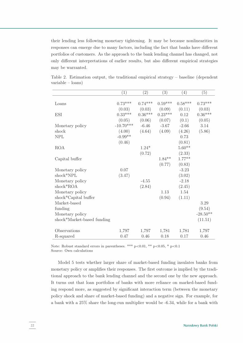
Narodowy Bank Polski22
their lending less following monetary tightening. It may be because nonlinearities in
responses can emerge due to many factors, including the fact that banks have different
portfolios of customers. As the approach to the bank lending channel has changed, not
only different interpretations of earlier results, but also different empirical strategies
may be warranted.
Table 2. Estimation output, the traditional empirical strategy – baseline (dependentvariable – loans)
(1) (2) (3) (4) (5)
Loans 0.73*** 0.74*** 0.59*** 0.58*** 0.73***(0.03) (0.03) (0.09) (0.11) (0.03)
ESI 0.33*** 0.36*** 0.23*** 0.12 0.36***(0.05) (0.06) (0.07) (0.1) (0.05)
Monetary policy -10.70*** -6.46 -3.67 -2.66 3.14shock (4.00) (4.64) (4.09) (4.26) (5.86)NPL -0.99** 0.73
(0.46) (0.81)ROA 1.24* 5.60**
(0.72) (2.33)Capital buffer 1.84** 1.77**
(0.77) (0.83)Monetary policy 0.07 -3.23shock*NPL (3.47) (3.02)Monetary policy -4.55 -2.18shock*ROA (2.84) (2.45)Monetary policy 1.13 1.54shock*Capital buffer (0.94) (1.11)Market-based 3.29funding (9.54)Monetary policy -28.50**shock*Market-based funding (11.51)
Observations 1,797 1,797 1,781 1,781 1,797R-squared 0.47 0.46 0.18 0.17 0.46
Note: Robust standard errors in parentheses. *** pă0.01, ** pă0.05, * pă0.1Source: Own calculations
Model 5 tests whether larger share of market-based funding insulates banks from
monetary policy or amplifies their responses. The first outcome is implied by the tradi-
tional approach to the bank lending channel and the second one by the new approach.
It turns out that loan portfolios of banks with more reliance on marked-based fund-
ing respond more, as suggested by significant interaction term (between the monetary
policy shock and share of market-based funding) and a negative sign. For example, for
a bank with a 25% share the long-run multiplier would be -6.34, while for a bank with
22
a 75% share – -18.02 (again, this is a large estimate, but a given level of the monet-
ary policy shock can correspond to a change in the domestic interest rate many times
larger). Although it may also be a result of banks having different portfolios (with
different demand elasticities), it can also be interpreted as a sign that the development
of interbank markets rather supported, than attenuated the bank lending channel.
Finally, Table F provides a robustness check on the results above. The monetary
policy shock is replaced by the domestic interest rate. In this case, the interaction
term between a measure of monetary policy and ROA is statistically significant, but
with unexpected, negative sign. Other results remain qualitatively unchanged. A point
estimate for the interaction term between the domestic interest rate and the share of
market-based funding is now more reasonable, implying a 2.09% decrease in lending
following a 1 percentage point increase in the interest rate for a bank with a 25% share,
and a 6.28% decrease for a bank with a 75% share.
23

23NBP Working Paper No. 245
Results
their lending less following monetary tightening. It may be because nonlinearities in
responses can emerge due to many factors, including the fact that banks have different
portfolios of customers. As the approach to the bank lending channel has changed, not
only different interpretations of earlier results, but also different empirical strategies
may be warranted.
Table 2. Estimation output, the traditional empirical strategy – baseline (dependentvariable – loans)
(1) (2) (3) (4) (5)
Loans 0.73*** 0.74*** 0.59*** 0.58*** 0.73***(0.03) (0.03) (0.09) (0.11) (0.03)
ESI 0.33*** 0.36*** 0.23*** 0.12 0.36***(0.05) (0.06) (0.07) (0.1) (0.05)
Monetary policy -10.70*** -6.46 -3.67 -2.66 3.14shock (4.00) (4.64) (4.09) (4.26) (5.86)NPL -0.99** 0.73
(0.46) (0.81)ROA 1.24* 5.60**
(0.72) (2.33)Capital buffer 1.84** 1.77**
(0.77) (0.83)Monetary policy 0.07 -3.23shock*NPL (3.47) (3.02)Monetary policy -4.55 -2.18shock*ROA (2.84) (2.45)Monetary policy 1.13 1.54shock*Capital buffer (0.94) (1.11)Market-based 3.29funding (9.54)Monetary policy -28.50**shock*Market-based funding (11.51)
Observations 1,797 1,797 1,781 1,781 1,797R-squared 0.47 0.46 0.18 0.17 0.46
Note: Robust standard errors in parentheses. *** pă0.01, ** pă0.05, * pă0.1Source: Own calculations
Model 5 tests whether larger share of market-based funding insulates banks from
monetary policy or amplifies their responses. The first outcome is implied by the tradi-
tional approach to the bank lending channel and the second one by the new approach.
It turns out that loan portfolios of banks with more reliance on marked-based fund-
ing respond more, as suggested by significant interaction term (between the monetary
policy shock and share of market-based funding) and a negative sign. For example, for
a bank with a 25% share the long-run multiplier would be -6.34, while for a bank with
22
a 75% share – -18.02 (again, this is a large estimate, but a given level of the monet-
ary policy shock can correspond to a change in the domestic interest rate many times
larger). Although it may also be a result of banks having different portfolios (with
different demand elasticities), it can also be interpreted as a sign that the development
of interbank markets rather supported, than attenuated the bank lending channel.
Finally, Table F provides a robustness check on the results above. The monetary
policy shock is replaced by the domestic interest rate. In this case, the interaction
term between a measure of monetary policy and ROA is statistically significant, but
with unexpected, negative sign. Other results remain qualitatively unchanged. A point
estimate for the interaction term between the domestic interest rate and the share of
market-based funding is now more reasonable, implying a 2.09% decrease in lending
following a 1 percentage point increase in the interest rate for a bank with a 25% share,
and a 6.28% decrease for a bank with a 75% share.
23

Narodowy Bank Polski24
Chapter 5
5 Conclusion
The study proposed an empirical strategy to identify whether the effects of monet-
ary policy are amplified through its impact on bank balance sheet strength. Such a
mechanism is known as the bank lending channel of monetary policy transmission (as
reformulated by Disyatat, 2011) and does not require loans to be limited by central
bank money or deposits. Panel vector autoregressions with high frequency identifica-
tion, univariate panel regressions and counterfactual exercises were applied to data for
Poland. They showed that a monetary policy impulse increases non-performing loans,
and reduces bank profitability and a capital buffer. Weaker balance sheets, in turn, are
associated with lower lending growth. Overall, the mechanism accounts for about 23%
of a decrease in lending following a monetary policy impulse.
For comparison, results from the traditional, less direct strategy for identifying the
bank lending channel were shown as well. However, using this strategy would not lead
to the same conclusions. This is probably because it reveals nonlinearity in responses of
different groups of banks to monetary policy due to many factors, including differences
in portfolios of customers. As the approach to the bank lending channel has changed,
not only different interpretations of earlier results, but also different empirical strategies
may be warranted.
This is another piece of evidence showing that the financial accelerator works in
both non-financial and financial sector. In some cases it can make the interplay between
monetary and macroprudential policy non-trivial. On the one hand, for example, during
a boom associated with a positive credit gap systematic monetary and macroprudential
policy complement each other. On the other hand, following a monetary policy surprise
its effects are partially offset by systematic macroprudential policy. Coordination may
be needed for optimal outcomes.
For future research, it would be useful to extend the analysis to quantify the role
banks not only as an amplifier, but also as a source of shocks, using data from the
Senior loan officer opinion survey. Studies of Bassett et al. (2014) and Altavilla et al.
(2015) are examples of steps in this direction.
24
Appendix
Figure A. Macro data
Source: CBOE, Central Statistical Office, Datastream, European Commission, Kapuściński (2015),NBP, own calculations
Figure B. Micro data
Source: NBP, own calculations
25

25NBP Working Paper No. 245
Appendix
5 Conclusion
The study proposed an empirical strategy to identify whether the effects of monet-
ary policy are amplified through its impact on bank balance sheet strength. Such a
mechanism is known as the bank lending channel of monetary policy transmission (as
reformulated by Disyatat, 2011) and does not require loans to be limited by central
bank money or deposits. Panel vector autoregressions with high frequency identifica-
tion, univariate panel regressions and counterfactual exercises were applied to data for
Poland. They showed that a monetary policy impulse increases non-performing loans,
and reduces bank profitability and a capital buffer. Weaker balance sheets, in turn, are
associated with lower lending growth. Overall, the mechanism accounts for about 23%
of a decrease in lending following a monetary policy impulse.
For comparison, results from the traditional, less direct strategy for identifying the
bank lending channel were shown as well. However, using this strategy would not lead
to the same conclusions. This is probably because it reveals nonlinearity in responses of
different groups of banks to monetary policy due to many factors, including differences
in portfolios of customers. As the approach to the bank lending channel has changed,
not only different interpretations of earlier results, but also different empirical strategies
may be warranted.
This is another piece of evidence showing that the financial accelerator works in
both non-financial and financial sector. In some cases it can make the interplay between
monetary and macroprudential policy non-trivial. On the one hand, for example, during
a boom associated with a positive credit gap systematic monetary and macroprudential
policy complement each other. On the other hand, following a monetary policy surprise
its effects are partially offset by systematic macroprudential policy. Coordination may
be needed for optimal outcomes.
For future research, it would be useful to extend the analysis to quantify the role
banks not only as an amplifier, but also as a source of shocks, using data from the
Senior loan officer opinion survey. Studies of Bassett et al. (2014) and Altavilla et al.
(2015) are examples of steps in this direction.
24
Appendix
Figure A. Macro data
Source: CBOE, Central Statistical Office, Datastream, European Commission, Kapuściński (2015),NBP, own calculations
Figure B. Micro data
Source: NBP, own calculations
25

Narodowy Bank Polski26
Table A. Unit root tests – aggregate
Augmented Dickey & Phillips & Perron Kwiatkowski, Phillips,Fuller Schmidt & Shin
Level Differenced Level Differenced Level Differenced
ESI -2.66* -4.89*** -2.09 -4.89*** 0.17Monetary policy -2.01 -4.36*** -1.75 -4.37*** 0.69** 0.30shockDomestic interest -4.24*** -5.43*** 0.69** 0.36*rateGDP deflator -1.39 -2.84*** -1.50 -6.23*** 0.91*** 0.29House prices -1.12 -4.14*** -1.33 -8.03*** 0.66** 0.16Foreign interest -1.77 -3.84*** -1.97 -3.71*** 0.71** 0.10rateExchange rate -1.69 -5.57*** -1.17 -5.60*** 0.46*VIX -3.05** -3.04** 0.11Loans -1.16 -1.16 -0.65 -1.55 0.88*** 0.19NPL -2.29 -2.46** -1.09 -2.31** 0.57** 0.14ROA -2.01 -9.34*** -4.51*** 0.17Capital buffer -1.4 -8.94*** -1.35 -8.82*** 0.72** 0.10
Note: *** pă0.01, ** pă0.05, * pă0.1Source: Own calculations
Table B. Unit root tests – micro
Levin, Lin & Im, Pesaran &Chu Shin
Level Differenced Level Differenced
Loans -10.18*** -11.2***NPL -15.44*** -16.59***ROA -18.06*** -18.42***Capital buffer -6.39*** -4.48***
Note: *** pă0.01, ** pă0.05, * pă0.1Source: Own calculations
26
Figure C. Sample coverage
Source: NBP, own calculations
27

27NBP Working Paper No. 245
Appendix
Figure C. Sample coverage
Source: NBP, own calculations
27

Narodowy Bank Polski28
Figure D. Responses to monetary policy impulse – alternative: domestic interest ratesas an additional endogenous variable
Source: Own calculations
Figure E. Responses to monetary policy impulse – alternative: NPL only
Source: Own calculations
28
Figure F. Responses to monetary policy impulse – alternative: ROA only
Source: Own calculations
Figure G. Responses to monetary policy impulse – alternative: capital buffer only
Source: Own calculations
29

29NBP Working Paper No. 245
Appendix
Figure D. Responses to monetary policy impulse – alternative: domestic interest ratesas an additional endogenous variable
Source: Own calculations
Figure E. Responses to monetary policy impulse – alternative: NPL only
Source: Own calculations
28
Figure F. Responses to monetary policy impulse – alternative: ROA only
Source: Own calculations
Figure G. Responses to monetary policy impulse – alternative: capital buffer only
Source: Own calculations
29

Narodowy Bank Polski30
Figure H. Responses to monetary policy impulse – alternative: GDP deflator as anadditional exogenous variable
Source: Own calculations
Figure I. Responses to monetary policy impulse – alternative: house prices as an addi-tional exogenous variable
Source: Own calculations
30
Figure J. Responses to monetary policy impulse – alternative: foreign interest rate asan additional exogenous variable
Source: Own calculations
Figure K. Responses to monetary policy impulse – alternative: exchange rate as anadditional exogenous variable
Source: Own calculations
31
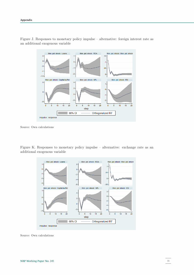
31NBP Working Paper No. 245
Appendix
Figure H. Responses to monetary policy impulse – alternative: GDP deflator as anadditional exogenous variable
Source: Own calculations
Figure I. Responses to monetary policy impulse – alternative: house prices as an addi-tional exogenous variable
Source: Own calculations
30
Figure J. Responses to monetary policy impulse – alternative: foreign interest rate asan additional exogenous variable
Source: Own calculations
Figure K. Responses to monetary policy impulse – alternative: exchange rate as anadditional exogenous variable
Source: Own calculations
31

Narodowy Bank Polski32
Figure L. Responses to monetary policy impulse – alternative: VIX as an additionalexogenous variable
Source: Own calculations
Figure M. Responses to monetary policy impulse – alternative: 2 lags
Source: Own calculations
32
Table C. Estimation output, univariate panel regressions – alternative: interest rateinstead of monetary policy shock (dependent variable – loans)
(1) (2) (3) (4)
Loans 0.72*** 0.73*** 0.63*** 0.61***(0.03) (0.03) (0.06) (0.06)
ESI 0.38*** 0.39*** 0.26*** 0.18**(0.06) (0.06) (0.07) (0.07)
Domestic interest -3.88*** -3.49*** 0.16 -0.01rate (0.94) (0.98) (1.36) (1.46)NPL -1.09** 0.04
(0.44) (0.51)ROA 1.42** 3.72***
(0.70) (1.09)Capital buffer 1.22*** 1.06***
(0.39) (0.37)
Observations 1,797 1,797 1,781 1,781R-squared 0.47 0.46 0.38 0.39
Note: Robust standard errors in parentheses. *** pă0.01, ** pă0.05, * pă0.1Source: Own calculations
33

33NBP Working Paper No. 245
Appendix
Figure L. Responses to monetary policy impulse – alternative: VIX as an additionalexogenous variable
Source: Own calculations
Figure M. Responses to monetary policy impulse – alternative: 2 lags
Source: Own calculations
32
Table C. Estimation output, univariate panel regressions – alternative: interest rateinstead of monetary policy shock (dependent variable – loans)
(1) (2) (3) (4)
Loans 0.72*** 0.73*** 0.63*** 0.61***(0.03) (0.03) (0.06) (0.06)
ESI 0.38*** 0.39*** 0.26*** 0.18**(0.06) (0.06) (0.07) (0.07)
Domestic interest -3.88*** -3.49*** 0.16 -0.01rate (0.94) (0.98) (1.36) (1.46)NPL -1.09** 0.04
(0.44) (0.51)ROA 1.42** 3.72***
(0.70) (1.09)Capital buffer 1.22*** 1.06***
(0.39) (0.37)
Observations 1,797 1,797 1,781 1,781R-squared 0.47 0.46 0.38 0.39
Note: Robust standard errors in parentheses. *** pă0.01, ** pă0.05, * pă0.1Source: Own calculations
33
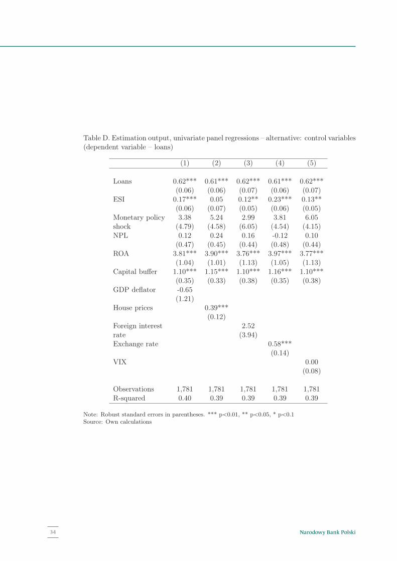
Narodowy Bank Polski34
Table D. Estimation output, univariate panel regressions – alternative: control variables(dependent variable – loans)
(1) (2) (3) (4) (5)
Loans 0.62*** 0.61*** 0.62*** 0.61*** 0.62***(0.06) (0.06) (0.07) (0.06) (0.07)
ESI 0.17*** 0.05 0.12** 0.23*** 0.13**(0.06) (0.07) (0.05) (0.06) (0.05)
Monetary policy 3.38 5.24 2.99 3.81 6.05shock (4.79) (4.58) (6.05) (4.54) (4.15)NPL 0.12 0.24 0.16 -0.12 0.10
(0.47) (0.45) (0.44) (0.48) (0.44)ROA 3.81*** 3.90*** 3.76*** 3.97*** 3.77***
(1.04) (1.01) (1.13) (1.05) (1.13)Capital buffer 1.10*** 1.15*** 1.10*** 1.16*** 1.10***
(0.35) (0.33) (0.38) (0.35) (0.38)GDP deflator -0.65
(1.21)House prices 0.39***
(0.12)Foreign interest 2.52rate (3.94)Exchange rate 0.58***
(0.14)VIX 0.00
(0.08)
Observations 1,781 1,781 1,781 1,781 1,781R-squared 0.40 0.39 0.39 0.39 0.39
Note: Robust standard errors in parentheses. *** pă0.01, ** pă0.05, * pă0.1Source: Own calculations
34
Table E. Estimation output, univariate panel regressions – alternative: 2 lags (depend-ent variable – loans)
(1) (2) (3) (4)
Loans 0.62*** 0.61*** 0.55*** 0.55***(0.03) (0.03) (0.04) (0.04)
ESI 0.20*** 0.18*** 0.16*** 0.14***(0.03) (0.03) (0.03) (0.04)
Monetary policy 1.08 0.49 3.15 4.09*shock (2.50) (2.38) (2.16) (2.20)NPL 0.34 0.50*
(0.32) (0.27)ROA 0.56 1.70***
(0.41) (0.56)Capital buffer 0.56*** 0.55***
(0.21) (0.21)
Observations 1,881 1,881 1,865 1,865R-squared 0.40 0.40 0.39 0.39
Note: Robust standard errors in parentheses. *** pă0.01, ** pă0.05, * pă0.1Source: Own calculations
35
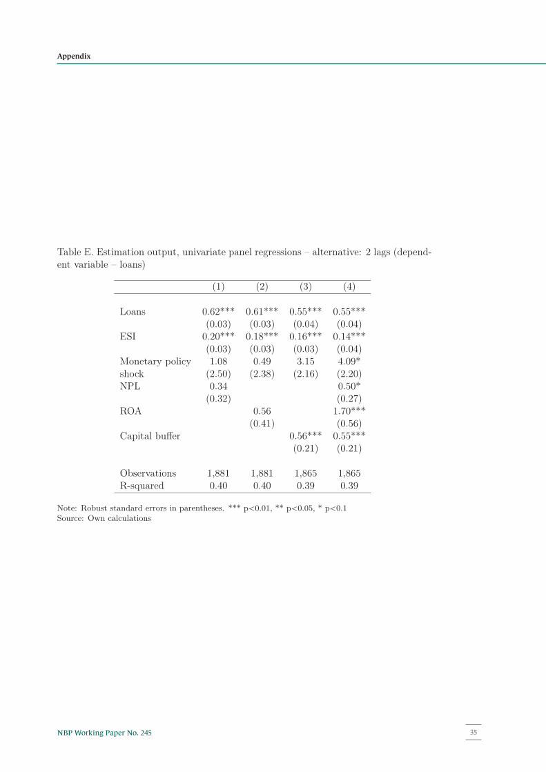
35NBP Working Paper No. 245
Appendix
Table D. Estimation output, univariate panel regressions – alternative: control variables(dependent variable – loans)
(1) (2) (3) (4) (5)
Loans 0.62*** 0.61*** 0.62*** 0.61*** 0.62***(0.06) (0.06) (0.07) (0.06) (0.07)
ESI 0.17*** 0.05 0.12** 0.23*** 0.13**(0.06) (0.07) (0.05) (0.06) (0.05)
Monetary policy 3.38 5.24 2.99 3.81 6.05shock (4.79) (4.58) (6.05) (4.54) (4.15)NPL 0.12 0.24 0.16 -0.12 0.10
(0.47) (0.45) (0.44) (0.48) (0.44)ROA 3.81*** 3.90*** 3.76*** 3.97*** 3.77***
(1.04) (1.01) (1.13) (1.05) (1.13)Capital buffer 1.10*** 1.15*** 1.10*** 1.16*** 1.10***
(0.35) (0.33) (0.38) (0.35) (0.38)GDP deflator -0.65
(1.21)House prices 0.39***
(0.12)Foreign interest 2.52rate (3.94)Exchange rate 0.58***
(0.14)VIX 0.00
(0.08)
Observations 1,781 1,781 1,781 1,781 1,781R-squared 0.40 0.39 0.39 0.39 0.39
Note: Robust standard errors in parentheses. *** pă0.01, ** pă0.05, * pă0.1Source: Own calculations
34
Table E. Estimation output, univariate panel regressions – alternative: 2 lags (depend-ent variable – loans)
(1) (2) (3) (4)
Loans 0.62*** 0.61*** 0.55*** 0.55***(0.03) (0.03) (0.04) (0.04)
ESI 0.20*** 0.18*** 0.16*** 0.14***(0.03) (0.03) (0.03) (0.04)
Monetary policy 1.08 0.49 3.15 4.09*shock (2.50) (2.38) (2.16) (2.20)NPL 0.34 0.50*
(0.32) (0.27)ROA 0.56 1.70***
(0.41) (0.56)Capital buffer 0.56*** 0.55***
(0.21) (0.21)
Observations 1,881 1,881 1,865 1,865R-squared 0.40 0.40 0.39 0.39
Note: Robust standard errors in parentheses. *** pă0.01, ** pă0.05, * pă0.1Source: Own calculations
35

Narodowy Bank Polski36
Table F. Estimation output, the traditional empirical strategy – alternative: interestrate instead of monetary policy shock (dependent variable – loans)
(1) (2) (3) (4) (5)
Loans 0.72*** 0.73*** 0.53*** 0.50* 0.71***(0.03) (0.03) (0.20) (0.28) (0.03)
ESI 0.37*** 0.41*** 0.15 -0.01 0.4***(0.05) (0.06) (0.16) (0.28) (0.05)
Domestic interest -4.29*** -1.79 -2.86* -0.87 0.40rate (0.96) (1.19) (1.50) (1.28) (1.37)NPL -1.10** 1.71
(0.44) (2.14)ROA 0.79 8.25
(0.72) (6.21)Capital buffer 2.85 3.20
(1.83) (2.56)Domestic interest 1.01 -1.15rate*NPL (0.74) (1.52)Domestic interest -1.96*** -2.29**rate*ROA (0.73) (1.16)Domestic interest 0.68 0.93rate*Capital buffer (0.57) (0.89)Market-based -0.20funding (9.76)Domestic interest -8.77***rate*Market-based funding (2.76)
Observations 1,797 1,797 1,781 1,781 1,797R-squared 0.47 0.47 . . 0.47
Note: Robust standard errors in parentheses. *** pă0.01, ** pă0.05, * pă0.1Source: Own calculations
36
References
Abrigo, M. R. and I. Love (2015). Estimation of Panel Vector Autoregression in Stata:
a Package of Programs. mimeo.
Altavilla, C., M. Darracq Paries, and G. Nicoletti (2015). Loan supply, credit markets
and the euro area financial crisis. Working Paper Series 1861, European Central
Bank.
Altunbas, Y., O. Fazylov, and P. Molyneux (2002). Evidence on the bank lending
channel in Europe. Journal of Banking & Finance 26 (11), 2093–2110.
Altunbas, Y., L. Gambacorta, and D. Marques-Ibanez (2009). Securitisation and the
bank lending channel. European Economic Review 53 (8), 996–1009.
Altunbas, Y., L. Gambacorta, and D. Marques-Ibanez (2010). Bank risk and monetary
policy. Journal of Financial Stability 6 (3), 121–129.
Bagliano, F. C. and C. A. Favero (1999). Information from financial markets and VAR
measures of monetary policy. European Economic Review 43 (4-6), 825–837.
Barakchian, S. M. and C. Crowe (2013). Monetary policy matters: Evidence from new
shocks data. Journal of Monetary Economics 60 (8), 950–966.
Bassett, W. F., M. B. Chosak, J. C. Driscoll, and E. Zakrajsek (2014). Changes in bank
lending standards and the macroeconomy. Journal of Monetary Economics 62 (C),
23–40.
Bernanke, B. S. (2007). The financial accelerator and the credit channel. Speech 296,
Board of Governors of the Federal Reserve System (U.S.).
Bernanke, B. S. and A. S. Blinder (1988). Credit, Money, and Aggregate Demand.
American Economic Review 78 (2), 435–39.
Bernanke, B. S. and M. Gertler (1995). Inside the Black Box: The Credit Channel of
Monetary Policy Transmission. Journal of Economic Perspectives 9 (4), 27–48.
Bernanke, B. S., M. Gertler, and S. Gilchrist (1999). The financial accelerator in
a quantitative business cycle framework. In J. B. Taylor and M. Woodford (Eds.),
Handbook of Macroeconomics, Volume 1 of Handbook of Macroeconomics, Chapter 21,
pp. 1341–1393. Elsevier.
Biggs, M., T. Mayer, and A. Pick (2009). Credit and economic recovery. DNB Working
Papers 218, Netherlands Central Bank, Research Department.
37

37NBP Working Paper No. 245
References
Table F. Estimation output, the traditional empirical strategy – alternative: interestrate instead of monetary policy shock (dependent variable – loans)
(1) (2) (3) (4) (5)
Loans 0.72*** 0.73*** 0.53*** 0.50* 0.71***(0.03) (0.03) (0.20) (0.28) (0.03)
ESI 0.37*** 0.41*** 0.15 -0.01 0.4***(0.05) (0.06) (0.16) (0.28) (0.05)
Domestic interest -4.29*** -1.79 -2.86* -0.87 0.40rate (0.96) (1.19) (1.50) (1.28) (1.37)NPL -1.10** 1.71
(0.44) (2.14)ROA 0.79 8.25
(0.72) (6.21)Capital buffer 2.85 3.20
(1.83) (2.56)Domestic interest 1.01 -1.15rate*NPL (0.74) (1.52)Domestic interest -1.96*** -2.29**rate*ROA (0.73) (1.16)Domestic interest 0.68 0.93rate*Capital buffer (0.57) (0.89)Market-based -0.20funding (9.76)Domestic interest -8.77***rate*Market-based funding (2.76)
Observations 1,797 1,797 1,781 1,781 1,797R-squared 0.47 0.47 . . 0.47
Note: Robust standard errors in parentheses. *** pă0.01, ** pă0.05, * pă0.1Source: Own calculations
36
References
Abrigo, M. R. and I. Love (2015). Estimation of Panel Vector Autoregression in Stata:
a Package of Programs. mimeo.
Altavilla, C., M. Darracq Paries, and G. Nicoletti (2015). Loan supply, credit markets
and the euro area financial crisis. Working Paper Series 1861, European Central
Bank.
Altunbas, Y., O. Fazylov, and P. Molyneux (2002). Evidence on the bank lending
channel in Europe. Journal of Banking & Finance 26 (11), 2093–2110.
Altunbas, Y., L. Gambacorta, and D. Marques-Ibanez (2009). Securitisation and the
bank lending channel. European Economic Review 53 (8), 996–1009.
Altunbas, Y., L. Gambacorta, and D. Marques-Ibanez (2010). Bank risk and monetary
policy. Journal of Financial Stability 6 (3), 121–129.
Bagliano, F. C. and C. A. Favero (1999). Information from financial markets and VAR
measures of monetary policy. European Economic Review 43 (4-6), 825–837.
Barakchian, S. M. and C. Crowe (2013). Monetary policy matters: Evidence from new
shocks data. Journal of Monetary Economics 60 (8), 950–966.
Bassett, W. F., M. B. Chosak, J. C. Driscoll, and E. Zakrajsek (2014). Changes in bank
lending standards and the macroeconomy. Journal of Monetary Economics 62 (C),
23–40.
Bernanke, B. S. (2007). The financial accelerator and the credit channel. Speech 296,
Board of Governors of the Federal Reserve System (U.S.).
Bernanke, B. S. and A. S. Blinder (1988). Credit, Money, and Aggregate Demand.
American Economic Review 78 (2), 435–39.
Bernanke, B. S. and M. Gertler (1995). Inside the Black Box: The Credit Channel of
Monetary Policy Transmission. Journal of Economic Perspectives 9 (4), 27–48.
Bernanke, B. S., M. Gertler, and S. Gilchrist (1999). The financial accelerator in
a quantitative business cycle framework. In J. B. Taylor and M. Woodford (Eds.),
Handbook of Macroeconomics, Volume 1 of Handbook of Macroeconomics, Chapter 21,
pp. 1341–1393. Elsevier.
Biggs, M., T. Mayer, and A. Pick (2009). Credit and economic recovery. DNB Working
Papers 218, Netherlands Central Bank, Research Department.
37

Narodowy Bank Polski38
Bluwstein, K. and F. Canova (2015). Beggar-thy-neighbor? The international effects
of ECB unconventional monetary policy measures. CEPR Discussion Papers 10856,
C.E.P.R. Discussion Papers.
Borio, C. and P. Disyatat (2010). Unconventional Monetary Policies: An Appraisal.
Manchester School 78 (s1), 53–89.
Borio, C. and H. Zhu (2012). Capital regulation, risk-taking and monetary policy: A
missing link in the transmission mechanism? Journal of Financial Stability 8 (4),
236–251.
Borio, C. E. V. (1997). Monetary policy operating procedures in industrial countries.
BIS Working Papers 40, Bank for International Settlements.
Breitenlechner, M. and J. Scharler (2015). The Bank Lending Channel and the Mar-
ket for Banks’ Funding: Demand for Non-reservable Deposits or Endogenous Risk
Premia. mimeo.
Brunnermeier, M. K. and Y. Sannikov (2016). The I Theory of Money. mimeo.
Brzoza-Brzezina, M. (2014). Financial Frictions and Macroprudential Policy. Interna-
tional Journal of Central Banking 10 (2), 249–261.
Carpenter, S. and S. Demiralp (2012). Money, reserves, and the transmission of mon-
etary policy: Does the money multiplier exist? Journal of Macroeconomics 34 (1),
59–75.
Cetorelli, N. and L. S. Goldberg (2008). Banking Globalization, Monetary Transmis-
sion, and the Lending Channel. NBER Working Papers 14101, National Bureau of
Economic Research, Inc.
Chami, R. and T. F. Cosimano (2010). Monetary policy with a touch of Basel. Journal
of Economics and Business 62 (3), 161–175.
Chmielewski, T. (2005). Bank risks, risk preferences and lending. MPRA Paper 5131,
University Library of Munich, Germany.
de Haan, L., J. W. van den End, and P. Vermeulen (2015). Lenders on the storm of
wholesale funding shocks: Saved by the central bank? DNB Working Papers 456,
Netherlands Central Bank, Research Department.
Disyatat, P. (2008). Monetary policy implementation: Misconceptions and their con-
sequences. BIS Working Papers 269, Bank for International Settlements.
Disyatat, P. (2011). The Bank Lending Channel Revisited. Journal of Money, Credit
and Banking 43 (4), 711–734.
38
Ehrmann, M., L. Gambacorta, J. Martinez Pages, P. Sevestre, and A. Worms (2001).
Financial systems and the role of banks in monetary policy transmission in the euro
area. Working Paper Series 0105, European Central Bank.
Gambacorta, L. (2005). Inside the bank lending channel. European Economic Re-
view 49 (7), 1737–1759.
Gambacorta, L. (2008). How do banks set interest rates? European Economic Re-
view 52 (5), 792–819.
Gertler, M. and P. Karadi (2015). Monetary Policy Surprises, Credit Costs, and Eco-
nomic Activity. American Economic Journal: Macroeconomics 7 (1), 44–76.
Goodhart, C. A. E. (2009). The Continuing Muddles of Monetary Theory: A Steadfast
Refusal to Face Facts. Economica 76 (s1), 821–830.
Gurkaynak, R. S., B. Sack, and E. Swanson (2005). Do Actions Speak Louder Than
Words? The Response of Asset Prices to Monetary Policy Actions and Statements.
International Journal of Central Banking 1 (1).
Havrylchyk, O. and E. Jurzyk (2005). Does the bank lending channel work in a trans-
ition economy? A case of Poland. European University Viadrina, mimeo.
Holmstrom, B. and J. Tirole (1997). Financial Intermediation, Loanable Funds, and
The Real Sector. The Quarterly Journal of Economics 112 (3), 663–691.
Hosono, K. and D. Miyakawa (2014). Business Cycles, Monetary Policy, and Bank
Lending: Identifying the bank balance sheet channel with firm-bank match-level loan
data. Discussion papers 14026, Research Institute of Economy, Trade and Industry
(RIETI).
Igan, D., A. N. Kabundi, F. N. D. Simone, and N. T. Tamirisa (2013). Monetary Policy
and Balance Sheets. IMF Working Papers 13/158, International Monetary Fund.
IMF (2013). Republic of Poland; Technical Note on Impaired Loans. IMF Staff Country
Reports 13/373, International Monetary Fund.
Jakab, Z. and M. Kumhof (2015). Banks are not intermediaries of loanable funds – and
why this matters. Bank of England working papers 529, Bank of England.
Kapuściński, M. (2015). Monetary policy and financial asset prices in Poland. NBP
Working Paper No. 216, Narodowy Bank Polski.
Kapuściński, M., A. Kociecki, H. Kowalczyk, T. Lyziak, J. Przystupa, E. Stanislawska,
A. Sznajderska, and E. Wróbel (2016). Monetary policy transmission mechanism in
Poland. What do we know in 2015? NBP Working Paper, Narodowy Bank Polski.
39

39NBP Working Paper No. 245
References
Bluwstein, K. and F. Canova (2015). Beggar-thy-neighbor? The international effects
of ECB unconventional monetary policy measures. CEPR Discussion Papers 10856,
C.E.P.R. Discussion Papers.
Borio, C. and P. Disyatat (2010). Unconventional Monetary Policies: An Appraisal.
Manchester School 78 (s1), 53–89.
Borio, C. and H. Zhu (2012). Capital regulation, risk-taking and monetary policy: A
missing link in the transmission mechanism? Journal of Financial Stability 8 (4),
236–251.
Borio, C. E. V. (1997). Monetary policy operating procedures in industrial countries.
BIS Working Papers 40, Bank for International Settlements.
Breitenlechner, M. and J. Scharler (2015). The Bank Lending Channel and the Mar-
ket for Banks’ Funding: Demand for Non-reservable Deposits or Endogenous Risk
Premia. mimeo.
Brunnermeier, M. K. and Y. Sannikov (2016). The I Theory of Money. mimeo.
Brzoza-Brzezina, M. (2014). Financial Frictions and Macroprudential Policy. Interna-
tional Journal of Central Banking 10 (2), 249–261.
Carpenter, S. and S. Demiralp (2012). Money, reserves, and the transmission of mon-
etary policy: Does the money multiplier exist? Journal of Macroeconomics 34 (1),
59–75.
Cetorelli, N. and L. S. Goldberg (2008). Banking Globalization, Monetary Transmis-
sion, and the Lending Channel. NBER Working Papers 14101, National Bureau of
Economic Research, Inc.
Chami, R. and T. F. Cosimano (2010). Monetary policy with a touch of Basel. Journal
of Economics and Business 62 (3), 161–175.
Chmielewski, T. (2005). Bank risks, risk preferences and lending. MPRA Paper 5131,
University Library of Munich, Germany.
de Haan, L., J. W. van den End, and P. Vermeulen (2015). Lenders on the storm of
wholesale funding shocks: Saved by the central bank? DNB Working Papers 456,
Netherlands Central Bank, Research Department.
Disyatat, P. (2008). Monetary policy implementation: Misconceptions and their con-
sequences. BIS Working Papers 269, Bank for International Settlements.
Disyatat, P. (2011). The Bank Lending Channel Revisited. Journal of Money, Credit
and Banking 43 (4), 711–734.
38
Ehrmann, M., L. Gambacorta, J. Martinez Pages, P. Sevestre, and A. Worms (2001).
Financial systems and the role of banks in monetary policy transmission in the euro
area. Working Paper Series 0105, European Central Bank.
Gambacorta, L. (2005). Inside the bank lending channel. European Economic Re-
view 49 (7), 1737–1759.
Gambacorta, L. (2008). How do banks set interest rates? European Economic Re-
view 52 (5), 792–819.
Gertler, M. and P. Karadi (2015). Monetary Policy Surprises, Credit Costs, and Eco-
nomic Activity. American Economic Journal: Macroeconomics 7 (1), 44–76.
Goodhart, C. A. E. (2009). The Continuing Muddles of Monetary Theory: A Steadfast
Refusal to Face Facts. Economica 76 (s1), 821–830.
Gurkaynak, R. S., B. Sack, and E. Swanson (2005). Do Actions Speak Louder Than
Words? The Response of Asset Prices to Monetary Policy Actions and Statements.
International Journal of Central Banking 1 (1).
Havrylchyk, O. and E. Jurzyk (2005). Does the bank lending channel work in a trans-
ition economy? A case of Poland. European University Viadrina, mimeo.
Holmstrom, B. and J. Tirole (1997). Financial Intermediation, Loanable Funds, and
The Real Sector. The Quarterly Journal of Economics 112 (3), 663–691.
Hosono, K. and D. Miyakawa (2014). Business Cycles, Monetary Policy, and Bank
Lending: Identifying the bank balance sheet channel with firm-bank match-level loan
data. Discussion papers 14026, Research Institute of Economy, Trade and Industry
(RIETI).
Igan, D., A. N. Kabundi, F. N. D. Simone, and N. T. Tamirisa (2013). Monetary Policy
and Balance Sheets. IMF Working Papers 13/158, International Monetary Fund.
IMF (2013). Republic of Poland; Technical Note on Impaired Loans. IMF Staff Country
Reports 13/373, International Monetary Fund.
Jakab, Z. and M. Kumhof (2015). Banks are not intermediaries of loanable funds – and
why this matters. Bank of England working papers 529, Bank of England.
Kapuściński, M. (2015). Monetary policy and financial asset prices in Poland. NBP
Working Paper No. 216, Narodowy Bank Polski.
Kapuściński, M., A. Kociecki, H. Kowalczyk, T. Lyziak, J. Przystupa, E. Stanislawska,
A. Sznajderska, and E. Wróbel (2016). Monetary policy transmission mechanism in
Poland. What do we know in 2015? NBP Working Paper, Narodowy Bank Polski.
39

Narodowy Bank Polski40
Kashyap, A. and J. C. Stein (1993). Monetary Policy and Bank Lending. NBER
Working Papers 4317, National Bureau of Economic Research, Inc.
Kashyap, A. K. and J. C. Stein (1995). The impact of monetary policy on bank balance
sheets. Carnegie-Rochester Conference Series on Public Policy 42 (1), 151–195.
Kashyap, A. K. and J. C. Stein (2000). What Do a Million Observations on Banks Say
about the Transmission of Monetary Policy? American Economic Review 90 (3),
407–428.
Kishan, R. P. and T. P. Opiela (2000). Bank Size, Bank Capital, and the Bank Lending
Channel. Journal of Money, Credit and Banking 32 (1), 121–41.
Kishan, R. P. and T. P. Opiela (2006). Bank capital and loan asymmetry in the
transmission of monetary policy. Journal of Banking & Finance 30 (1), 259–285.
Kishan, R. P. and T. P. Opiela (2012). Monetary Policy, Bank Lending, and the
Risk-Pricing Channel. Journal of Money, Credit and Banking 44 (4), 573–602.
Kozak, S. (2013). Consolidation of the banking sector in Poland in 1989-2013 in com-
parison with the structural changes of the banking sector in the USA and the EU.
NBP Working Paper No. 166, Narodowy Bank Polski.
Matousek, R. and N. Sarantis (2009). The bank lending channel and monetary trans-
mission in Central and Eastern European countries. Journal of Comparative Eco-
nomics 37 (2), 321–334.
McLeay, M., A. Radia, and R. Thomas (2014). Money creation in the modern economy.
Bank of England Quarterly Bulletin 54 (1), 14–27.
Meh, C. (2011). Bank Balance Sheets, Deleveraging and the Transmission Mechanism.
Bank of Canada Review 2011 (Summer), 23–34.
Opiela, T. P. (2008). Differential Deposit Guarantees And The Effect Of Monetary
Policy On Bank Lending. Economic Inquiry 46 (4), 610–623.
Passari, E. and H. Rey (2015). Financial Flows and the International Monetary System.
Economic Journal 0 (584), 675–698.
Pawłowska, M. and E. Wróbel (2002). Monetary transmission in Poland: some evidence
on interest rate and credit channels. National Bank of Poland Working Papers 24,
National Bank of Poland, Economic Institute.
Peek, J. and E. S. Rosengren (1995). Bank lending and the transmission of monetary
policy. In Conference series-Federal Reserve Bank of Boston, Volume 39, pp. 47–68.
Federal Reserve Bank of Boston.
40
Peek, J. and E. S. Rosengren (2013). The role of banks in the transmission of monetary
policy. Public Policy Discussion Paper 13-5, Federal Reserve Bank of Boston.
Romer, C. D. and D. H. Romer (1990). New Evidence on the Monetary Transmission
Mechanism. Brookings Papers on Economic Activity 21 (1), 149–214.
Rudebusch, G. D. (1998). Do Measures of Monetary Policy in a VAR Make Sense?
International Economic Review 39 (4), 907–31.
Serwa, D. and P. Wdowiński (2015). Zaleznosci miedzy sektorem bankowym i realnym:
strukturalny model VAR (Interrelations between the banking and the real sector: a
structural VAR model). mimeo.
Shin, H. S. (2009). Reflections on Northern Rock: The Bank Run That Heralded the
Global Financial Crisis. Journal of Economic Perspectives 23 (1), 101–19.
Stein, J. C. (1998). An Adverse-Selection Model of Bank Asset and Liability Manage-
ment with Implications for the Transmission of Monetary Policy. RAND Journal of
Economics 29 (3), 466–486.
Stiglitz, J. and B. Greenwald (2003). Towards a New Paradigm in Monetary Economics.
Number 9780521008051 in Cambridge Books. Cambridge University Press.
Van den Heuvel, S. (2006). The Bank Capital Channel of Monetary Policy. 2006
Meeting Papers 512, Society for Economic Dynamics.
Wdowiński, P. (2014). Makroekonomiczne czynniki ryzyka kredytowego w sektorze
bankowym w Polsce (Macroeconomic factors of the credit risk in the banking sector
in Poland). Gospodarka Narodowa (4), 55–77.
Werner, R. A. (2014). Can banks individually create money out of nothing? The
theories and the empirical evidence. International Review of Financial Analysis 36,
1 – 19.
Werner, R. A. (2015). A lost century in economics: Three theories of banking and the
conclusive evidence. International Review of Financial Analysis .
41

41NBP Working Paper No. 245
References
Kashyap, A. and J. C. Stein (1993). Monetary Policy and Bank Lending. NBER
Working Papers 4317, National Bureau of Economic Research, Inc.
Kashyap, A. K. and J. C. Stein (1995). The impact of monetary policy on bank balance
sheets. Carnegie-Rochester Conference Series on Public Policy 42 (1), 151–195.
Kashyap, A. K. and J. C. Stein (2000). What Do a Million Observations on Banks Say
about the Transmission of Monetary Policy? American Economic Review 90 (3),
407–428.
Kishan, R. P. and T. P. Opiela (2000). Bank Size, Bank Capital, and the Bank Lending
Channel. Journal of Money, Credit and Banking 32 (1), 121–41.
Kishan, R. P. and T. P. Opiela (2006). Bank capital and loan asymmetry in the
transmission of monetary policy. Journal of Banking & Finance 30 (1), 259–285.
Kishan, R. P. and T. P. Opiela (2012). Monetary Policy, Bank Lending, and the
Risk-Pricing Channel. Journal of Money, Credit and Banking 44 (4), 573–602.
Kozak, S. (2013). Consolidation of the banking sector in Poland in 1989-2013 in com-
parison with the structural changes of the banking sector in the USA and the EU.
NBP Working Paper No. 166, Narodowy Bank Polski.
Matousek, R. and N. Sarantis (2009). The bank lending channel and monetary trans-
mission in Central and Eastern European countries. Journal of Comparative Eco-
nomics 37 (2), 321–334.
McLeay, M., A. Radia, and R. Thomas (2014). Money creation in the modern economy.
Bank of England Quarterly Bulletin 54 (1), 14–27.
Meh, C. (2011). Bank Balance Sheets, Deleveraging and the Transmission Mechanism.
Bank of Canada Review 2011 (Summer), 23–34.
Opiela, T. P. (2008). Differential Deposit Guarantees And The Effect Of Monetary
Policy On Bank Lending. Economic Inquiry 46 (4), 610–623.
Passari, E. and H. Rey (2015). Financial Flows and the International Monetary System.
Economic Journal 0 (584), 675–698.
Pawłowska, M. and E. Wróbel (2002). Monetary transmission in Poland: some evidence
on interest rate and credit channels. National Bank of Poland Working Papers 24,
National Bank of Poland, Economic Institute.
Peek, J. and E. S. Rosengren (1995). Bank lending and the transmission of monetary
policy. In Conference series-Federal Reserve Bank of Boston, Volume 39, pp. 47–68.
Federal Reserve Bank of Boston.
40
Peek, J. and E. S. Rosengren (2013). The role of banks in the transmission of monetary
policy. Public Policy Discussion Paper 13-5, Federal Reserve Bank of Boston.
Romer, C. D. and D. H. Romer (1990). New Evidence on the Monetary Transmission
Mechanism. Brookings Papers on Economic Activity 21 (1), 149–214.
Rudebusch, G. D. (1998). Do Measures of Monetary Policy in a VAR Make Sense?
International Economic Review 39 (4), 907–31.
Serwa, D. and P. Wdowiński (2015). Zaleznosci miedzy sektorem bankowym i realnym:
strukturalny model VAR (Interrelations between the banking and the real sector: a
structural VAR model). mimeo.
Shin, H. S. (2009). Reflections on Northern Rock: The Bank Run That Heralded the
Global Financial Crisis. Journal of Economic Perspectives 23 (1), 101–19.
Stein, J. C. (1998). An Adverse-Selection Model of Bank Asset and Liability Manage-
ment with Implications for the Transmission of Monetary Policy. RAND Journal of
Economics 29 (3), 466–486.
Stiglitz, J. and B. Greenwald (2003). Towards a New Paradigm in Monetary Economics.
Number 9780521008051 in Cambridge Books. Cambridge University Press.
Van den Heuvel, S. (2006). The Bank Capital Channel of Monetary Policy. 2006
Meeting Papers 512, Society for Economic Dynamics.
Wdowiński, P. (2014). Makroekonomiczne czynniki ryzyka kredytowego w sektorze
bankowym w Polsce (Macroeconomic factors of the credit risk in the banking sector
in Poland). Gospodarka Narodowa (4), 55–77.
Werner, R. A. (2014). Can banks individually create money out of nothing? The
theories and the empirical evidence. International Review of Financial Analysis 36,
1 – 19.
Werner, R. A. (2015). A lost century in economics: Three theories of banking and the
conclusive evidence. International Review of Financial Analysis .
41

www.nbp.pl