The Real Consequences of Bank Mortgage Lending … Real Consequences of Bank Mortgage Lending...
43
16-05 | May 11, 2016 The Real Consequences of Bank Mortgage Lending Standards Cindy M. Vojtech Federal Reserve Board [email protected] Benjamin S. Kay Office of Financial Research [email protected] John C. Driscoll Federal Reserve Board [email protected] The Office of Financial Research (OFR) Working Paper Series allows members of the OFR staff and their coauthors to disseminate preliminary research findings in a format intended to generate discussion and critical comments. Papers in the OFR Working Paper Series are works in progress and subject to revision. Views and opinions expressed are those of the authors and do not necessarily represent official positions or policy of the OFR or Treasury. Comments and suggestions for improvements are welcome and should be directed to the authors. OFR working papers may be quoted without additional permission.
-
Upload
hoangthuan -
Category
Documents
-
view
215 -
download
1
Transcript of The Real Consequences of Bank Mortgage Lending … Real Consequences of Bank Mortgage Lending...
16-05 | May 11, 2016
The Real Consequences of Bank Mortgage Lending Standards
Cindy M. Vojtech Federal Reserve Board [email protected]
Benjamin S. Kay Office of Financial Research [email protected]
John C. Driscoll Federal Reserve Board [email protected]
The Office of Financial Research (OFR) Working Paper Series allows members of the OFR staff and their coauthors to disseminate preliminary research findings in a format intended to generate discussion and critical comments. Papers in the OFR Working Paper Series are works in progress and subject to revision. Views and opinions expressed are those of the authors and do not necessarily represent official positions or policy of the OFR or Treasury. Comments and suggestions for improvements are welcome and should be directed to the authors. OFR working papers may be quoted without additional permission.
The Real Consequences of Bank Mortgage LendingStandards
Cindy M. Vojtech a, Benjamin S. Kay b, and John C. Driscoll a,∗
a bFederal Reserve Board Treasury, Office of Financial Research
May 11, 2016
Abstract
Bank loan underwriting standards are key determinants of credit availability. Tobetter understand what happens when bank loan officers change standards, we matchresponses from the Federal Reserve’s Senior Loan Officer Opinion Survey (SLOOS) withmortgage application information from the Home Mortgage Disclosure Act (HMDA)over the period from 1990 to 2013. HMDA data contain both accepted and deniedapplications, allowing us to observe changes in denial rates when loan officers reportchanging standards. Reports of tightened standards are associated with an increase ofabout 1 percentage point in denial rates (conditioning on changes in macroeconomicconditions and borrower credit quality), implying a reduction in aggregate mortgagecredit of about $690 million per quarter. Reports of easing standards, though lessfrequent over that period, are associated with a 1 percentage point decline in denialrates. Denial rate changes are larger for banks that hold most of their mortgageson portfolio (rather than securitizing them). Tighter standards are associated withabout 16 percent fewer high interest rate loans (a proxy for riskier loans). Applicationsrise at banks that report strengthening demand for mortgage loans. Metropolitanstatistical areas (MSAs) that have more exposure to SLOOS banks that have tightenedstandards have much lower delinquency rates two years following the tightening—suggesting that standards are an important determinant of the credit quality of bankloan portfolios. House prices also fall in MSAs that have exposure to SLOOS banksthat report tightening.
∗Corresponding author. Address: 20th and Constitution Ave. NW, Washington, DC 20551. E-mail:[email protected]. Phone: (202) 452-2628. This paper previously circulated under the title “WhatDo Loan Officers Do When They Change Standards and Terms?” We thank Sumit Agarwal, Man Cho,Masaki Mori, Jon Mondragon, and seminar participants at the Federal Reserve Board, the Office of Finan-cial Research, the Federal Housing Finance Agency, the Bundesbank, the Oesterreichische Nationalbank,LUMSA, and the IRES Symposium for helpful comments. We also thank Robert Avery and Neil Bhuttafor data identifying banks in the HMDA data and Mike Massare and Edward Kim for excellent researchassistance. The views expressed in this paper are those of the authors, and not necessarily those of theFederal Reserve Board, the Office of Financial Research, or their respective staffs.
1 Introduction
Researchers have long examined the extent to which commercial banks are a source of and
propagation mechanism for macroeconomic shocks.1 Recently, this topic has become partic-
ularly important, as excessively easy underwriting standards on residential real estate loans
have been implicated as a major cause of the financial crisis. Understanding how bank loan
underwriting standards affect real outcomes in loan markets and the macroeconomy more
broadly is thus of considerable interest.
One source of information on bank loan underwriting policies is the Federal Reserve’s
quarterly Senior Loan Officer Opinion Survey (SLOOS). The survey, which has been con-
ducted since the 1960s and has consistent questions available since the early 1990s, asks bank
loan officers to indicate how they have changed underwriting standards and terms on major
types of business and household loans. This paper is the first to match the (confidential)
individual bank responses from the SLOOS with mortgage application information from the
Home Mortgage Disclosure Act (HMDA). HMDA data contain information on applications
that were denied as well as those that were accepted; thus, we can observe changes in de-
nial rates—an important margin by which changes in credit standards can have an effect
on potential borrowers. We can also observe changes in the amounts for approved loans
and match those to reports on changes in loan terms. We match the data over a period
from 1990 until 2013, yielding about 4,600 bank-quarter observations. Other authors (for
example, Lown and Morgan (2006) and Bassett et al. (2014)) have found that SLOOS re-
sponses have predictive power for macroeconomic activity. By establishing what happens in
the mortgage market when SLOOS respondents report having changed standards or terms,
we provide quantitative estimates of how changes in standards contribute to changes in the
macroeconomy.
Estimating the relationship between standards and these outcome variables is confounded
1See, for example, King (1986), Bernanke and Blinder (1988), Romer and Romer (1990), Bernanke andLown (1991), Gertler and Gilchrist (1993), Kashyap and Stein (1994, 2000), Peek and Rosengren (1995a,b,2000), Driscoll (2004), Ashcraft (2005), and Gilchrist and Zakrajsek (2012).
1
by two endogeneity problems. First, potential applicants may choose to not apply when
they perceive that lending standards have tightened. This may be why denial rates are
not highly countercyclical. Second, the pool of potential applicants for a specific bank may
change in credit quality due to changes in standards by other banks or to changes in local
or macroeconomic factors.
We address these problems in two ways. First, we include both national and local mea-
sures of macroeconomic conditions. Second, we include characteristics of the borrower pool
to control for changes in credit quality.
We find that a loan officer’s report of tightening standards is associated with an increase
of about 1 percentage point in that bank’s mortgage loan denial rate. This corresponds to
an aggregate reduction in mortgage credit from banks of about $690 million per quarter just
through the direct channel of denial rates. Reports of easing standards, though less frequent
over our sample period, are associated with a 1 percentage point decline in denial rates.
Because securitization reduces the screening incentives of originators, we test if securiti-
zation changes the relationship between changes in standards and denial rates. We find that
the effects on denial rates are larger at banks that hold their loans on portfolio, rather than
securitizing them. This is consistent with this reduced screening incentive.
We also test the effects on the dollars of mortgage credit extended. We estimate that
mortgage credit falls by about 5 percent when standards tighten and rises by about 4 percent
when demand for such credit strengthens.
Because we expect standards to have a greater effect on marginal borrowers, we separately
test the effect of changes in standards on that population. In particular, we analyze high
interest rate loans—a proxy for subprime and other nontraditional mortgages. We find that
such loans fall significantly, about 16 percent, when SLOOS banks report tightening.
With regard to questions on changes in demand, applications at SLOOS banks rise when
the latter report increases in demand. In contrast, reports of changes in demand have a
much smaller or insignificant relationship with denial rates. Similarly, changes in standards
2

have little effect on the volume of applications.
We look at the relationship between changes in standards and loan performance. We find
that MSAs that have more exposure to SLOOS banks that tightened standards have much
lower delinquency rates two years following the tightening. This suggests that when banks
tighten standards they are successful in not extending credit to borrowers who will have
trouble repaying their debts. It also suggests that SLOOS credit standards are a leading
indicator of financial industry vulnerability to shocks.
Finally, we look at the impact of bank lending standards on local housing markets. We
find that, in MSAs with more exposure to SLOOS banks that have tightened standards,
house prices decline—as one would expect from the decline in approved mortgages in such
areas.
The rest of the paper proceeds as follows: the next section reviews related literature;
section 3 provides details on the data and empirical strategy; section 4 provides results; and
section 5 concludes.
2 Related Literature
Although the Federal Reserve has conducted the SLOOS since 1966, much of the research
on the behavior of loan officers is comparatively recent, in part because it is only since
1990 that the survey has consistently asked about changes in lending policies across credit
products. Schreft and Owens (1991) provides a history of the early SLOOS and the general
methodology that persists to the present. One line of research has used this data to explore
bank-loan officer agency problems. Udell (1989) shows that loan review serves to reduce
these problems. Stein (2002) argues that agency problems in part depend on the degree to
which the loan relies on soft information. This is in agreement with the empirical findings
of Berger et al. (2005), Liberti and Mian (2009), and Agarwal and Hauswald (2010). Heider
and Inderst (2012) develop an optimal contracting model for loan officers. Agarwal and
3
Ben-David (1991), Berg et al. (2013), Berg et al. (2014) and Cole et al. (2013) examine loan
officers’ incentives, the latter using a laboratory experiment. Wang (2015) estimates that
heterogeneity in risk preferences, screening ability, and belief about screening ability by loan
officers appear to distort loan officer behavior.
A smaller body of work has looked at the macroeconomic impact of loan officer behavior
by using the SLOOS, including Lown et al. (2000), Lown and Morgan (2006), Cunningham
(2006), and Bassett et al. (2014). That literature generally finds that changes in SLOOS
standards have predictive power for subsequent movements in both banking variables such
as loans and macroeconomic variables such as GDP. However, in principle, this could be
because loan officers are well-informed or because they have a significant impact given the
critical role of banks in the economy.
Our paper is most closely related to Bassett et al. (2014) and Cunningham (2006) which
try to distinguish these informational and causal channels. Bassett et al. (2014) exploit
bank level shifts in the supply of business loans to confirm that “adjusted changes in banks’
lending standards capture shifts in business loan supply.” Cunningham (2006) finds that
growth in aggregate real estate loans is not well predicted by SLOOS standards responses.
This suggests that loan officers responding to the survey are simply commenting on market
conditions rather than signaling changes in their own credit decisions. Our results contrast
sharply with Cunningham (2006). We find that standards and demand measures both have
a statistically and economically important effect on credit extension. In fact, the effects of
changes in standards are larger than those from changes in demand. One key reason for the
different results is we can match bank responses to bank changes in credit, which gives us
much greater statistical power and additionally allows for inter-bank effects. The two earlier
papers use “net percentage of respondents reporting tightening standards,” a measure that
treats all banks as changing standards identically. This is a problem if, for example, in a
two-bank market one eases and the other tightens standards. The net percentage in this
market is zero, but overall credit may increase as the easing lender attracts new borrowers
4
as well as cast-off applicants from the tightening lender.
Also closely related to our work is Del Giovane et al. (2011) which uses data from the
Eurosystem Bank Lending Survey to study supply and demand shifts in lending to enterprises
in Italy. However, they cannot externally validate that the survey responses are actually
shifts in supply and demand. In contrast, because we can study mortgage applications
distinctly from approved mortgage quantities, we validate that change in demand does drive
applications and can be treated as a shift in the demand curve.
3 Data and Empirical Strategy
3.1 Data
3.1.1 The Senior Loan Officer Opinion Survey (SLOOS)
The Federal Reserve’s Senior Loan Officer Opinion Survey on Bank Lending Practices has
polled banks about changes in their lending standards for major categories of loans to house-
holds and businesses since 1990:Q2 and about changes in demand for those loan categories
since 1990:Q3. The survey is usually conducted quarterly by the Federal Reserve Board, and
for the majority of our sample, nearly 60 U.S. commercial banks participate in each survey.2
The survey panel of domestic banks spans all Federal Reserve Districts, while balancing the
need to keep it heavily weighted toward large banks. The primary cause of sample attrition
is the acquisition of a respondent bank by another bank that already participates in the
survey. Thus, nonresponse selection bias in the respondents is likely to be limited.
Banks are asked to report whether they have changed their standards during the survey
2While the survey has been conducted since 1966, questions have been consistently asked only since1990. However, the demand question was not asked in 1991:Q2. Up to 24 U.S. branches and agencies offoreign banks also participate in the survey, though they do not answer questions about residential realestate loans, as such loans are generally not a large part of their business. The survey is voluntary, butbanks that are asked to participate in the survey almost always agree to do so. In 2012, the domesticpanel (covering all Federal Reserve Districts) was expanded to allow up to 80 banks and represented about70 percent of total assets at domestically chartered institutions. For more information on the survey, seewww.federalreserve.gov/boarddocs/SnLoanSurvey.
5
period (i.e., over the previous three months) on seven categories of core loans: commercial
and industrial, commercial real estate, residential mortgages to purchase homes, home equity
lines of credit, credit cards, auto, and consumer loans other than credit cards or auto loans.
They also are asked about changes in demand for these categories. For this paper, we use
only answers about residential mortgage loans because no comparable application data exist
for any of these other categories.3
The question about changes in standards is,
“Over the past three months, how have your bank’s credit standards for approving
applications from individuals for mortgage loans to purchase homes changed?”4
Similarly, the question about changes in demand is,
“Apart from normal seasonal variation, how has demand for mortgages to pur-
chase homes changed over the past three months? (Please consider only applica-
tions for new originations as opposed to applications for refinancing of existing
mortgages.)”5
Banks are asked to answer both questions using a five-point scale. In the case of stan-
dards, the scale is: 1=“eased considerably”; 2=“eased somewhat”; 3=“about unchanged”;
4=“tightened somewhat”; and 5=“tightened considerably.” For demand, “eased” and
“tightened” are replaced with “strengthened” and “weakened,” respectively.
As banks historically have been extremely unlikely to characterize their changes in stan-
dards or demand as having changed “considerably,” we use only two classifications for those
3Starting with the April 2007 survey, the respondents were asked about changes in standards and demandon residential mortgages by type of mortgage product (prime, nontraditional, or subprime). In constructingour series, we combine responses across mortgage types as follows. We code each of the three loan types as-1, 0, or 1, for easing, unchanged, or tightening, respectively. We sum across loan types. If the sum is ≤ −1,then aggregate series = −1. If the sum is zero, then we code the aggregate series as = 0. If the sum is ≥ 1,then the aggregate series = 1.
4See, for example, question 24 of the Senior Loan Officer Opinion Survey on Bank Lending Practices,April 2016 Edition, https://www.federalreserve.gov/boarddocs/snloansurvey/201605/table1.htm, accessedon 5/3/2016.
5Ibid, Question 25. The order and numbering of the questions changes from survey to survey but thetext does not.
6
variables, rather than the five possible answers available to survey respondents: a dummy
variable for whether standards have eased considerably or somewhat; and a dummy variable
for whether they have tightened considerably or somewhat (and similarly for demand).
Figure 1 plots two summary measures of changes in standards and demand over the
sample period. For the change in standards series (top panel), the bars show the fraction
of respondents reporting they have tightened standards (blue bars) as well as the fraction
reporting that they have eased standards (red bars). For the change in demand series
(bottom panel), the bars show the fraction of respondents reporting they have seen stronger
demand (blue bars) and the fraction reporting that they have seen weaker demand (red
bars). The resulting series match prevailing narrative accounts of the period. For example,
the standards series shows net easings for much of the early 2000s during the real estate
boom, followed by tightenings preceding and during the recession of 2007-2009. The data
also show several episodes when a significant number of banks were easing and tightening
standards contemporaneously.
3.1.2 The Home Mortgage Disclosure Act (HMDA)
The Home Mortgage Disclosure Act of 1975 is a disclosure law for mortgages and mortgage
applications. Most banks, savings and loan associations, credit unions, and consumer finance
companies are required to report under HMDA. Avery et al. (2007) estimate that the more
than 8,900 lenders then covered by the law accounted for approximately 80 percent of all
home lending nationwide in 2006.6HMDA requires lenders to collect and publicly disclose
information on housing-related applications. The mandatory reporting threshold for depos-
itory institutions has changed slightly over time, but includes almost all commercial banks
that originate mortgage loans. The threshold for data collection in 2015 was $44 million
in total assets.7 Any bank with assets above the threshold, with a branch in an MSA,
6Avery et al. (2007) provide an extensive discussion of HMDA data. The FFIEC website also provides ahistory: www.ffiec.gov/hmda/history2.htm.
7Domestic banks participating in the SLOOS must have at least $3 Billion in assets so this thresh-old does not eliminate any banks. See Supporting Statement for the Senior Loan Officer Opin-
7
and that originated at least one mortgage loan in the calendar year must file a HMDA re-
port.8 The Federal Reserve Board had rulemaking authority over the reporting form until
mid-2011. After that, rulemaking authority passed to the Consumer Financial Protection
Bureau (CFPB).
We match HMDA applications and SLOOS responses at the bank level for the period
between 1990 and 2013. In addition, HMDA respondents owned by a bank holding company
(BHC) are linked to the largest commercial bank (“lead bank”) within that organization.
These lead banks are often SLOOS respondents. Because the SLOOS sample is somewhat
limited in size (60 banks), respondents are generally selected as the largest banking subsidiary
in a BHC without duplicates in the same BHC.9
The action date on the HMDA form is used to link an application to a specific quarter.10
For each bank-quarter, the denial rate is calculated using only home purchase loan appli-
cations.11 To stay in the testing panel, a bank observation must have at least 30 purchase
applications in both the current quarter and the prior quarter. In addition, a bank must
have at least four quarters of testable data. The main testing panel averages 49 banks per
quarter.12
Figure 2 plots quartiles of the denial rate for our SLOOS panel of banks. Although the
ion Survey on Bank Lending Practices (FR 2018; OMB No. 7100–0058), Federal Reserve Board,http://www.federalreserve.gov/boarddocs/SnLoanSurvey/about.htm, Accessed May 3, 2016.
8For details of the filing requirements see Home Mortgage Disclosure Act Examination Procedures, Fed-eral Reserve Board, https://www.federalreserve.gov/boarddocs/caletters/2009/0910/09-10 attachment.pdf,accessed on May 3, 2016.
9It is believed that the standards and practices of loan officers are generally similar for banks that operatewithin the same BHC.
10We use a confidential version of HMDA that includes the action date, unlike in the publicly availabledata, which shows only the year a loan occurred. The action date is the closing date for originated loans,the withdrawal date for loans approved but withdrawn by the potential borrower, and the denial date fordenied loans.
11We exclude refinance and home improvement loans to match the SLOOS mortgage question. Otherexclusions from the HMDA applications include: multifamily, manufactured housing, pre-approvals, andnon-owner-occupied housing.
12While the SLOOS has approval to survey up to 60 banks per quarter for most of the time frame studied,on average, 57.3 banks responded between 1990:Q3 and 2013:Q4. Of those, 4.2 banks did not answer themortgage questions. Banks generally do not answer questions about loan types that are not core to theirbusiness model. Other decreases in observations are primarily due to the purchase application and four-quarter requirements. Recall that several banks were added in 2012.
8
rate is, as expected, countercyclical, it does not vary much over time; the median is generally
between 10 percent and 15 percent for much of the sample.
The only borrower credit characteristic in HMDA is reported income. We use this and
loan size to calculate a loan-to-income (LTI) ratio for each application. We then divide the
applications into LTI ratio buckets based on LTI quintile thresholds in 2002 (the sample mid-
point). There is also a missing LTI category for the relatively small number of applications
without reported income. We use the shares for each category as explanatory variables
(dropping the largest for collinearity) to control for changes in borrower characteristics of a
bank’s applicant pool. In principle, a higher LTI ratio should indicate a riskier application,
although several authors have raised concerns about the accuracy of reported income in
HMDA applications (e.g., Avery et al. (2011) and Mian and Sufi (2015)). Furthermore, this
ratio is limited in scope as it does not capture other debt the applicant may have (e.g., student
loans and credit cards). In general, unobservable credit characteristics may be negatively
correlated with observable ones conditional on application amount; high down payment and
high FICO score borrowers can expect to successfully borrow larger amounts conditional on
income.
For more information about the credit quality of a bank’s borrower pool, we use data from
Lender Processing Services (LPS) Applied Analytics (formerly known as McDash Analytics).
These data consist of mortgage loans currently being serviced by some of the nation’s largest
servicers. Loans in LPS represent approximately two-thirds all serviced residential mort-
gages. The data include updated FICO scores of the borrower and the current delinquency
status of the loan. Licensing restrictions prohibit the triple merge of LPS-HMDA-SLOOS
because the bank would be identifiable to the authors. As an alternative, we use geographic
data in HMDA and LPS to build borrower controls and to test MSA-level outcomes. Because
LPS data has improved coverage in later years, regressions using these data are confined to
the period 2005 to 2013.
Table 1 presents summary statistics for the testing panel. As shown in figure 1, reports
9
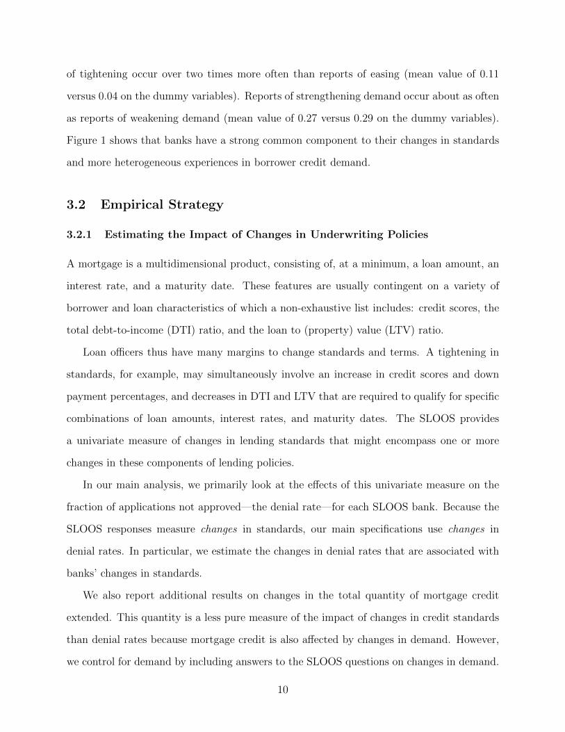
of tightening occur over two times more often than reports of easing (mean value of 0.11
versus 0.04 on the dummy variables). Reports of strengthening demand occur about as often
as reports of weakening demand (mean value of 0.27 versus 0.29 on the dummy variables).
Figure 1 shows that banks have a strong common component to their changes in standards
and more heterogeneous experiences in borrower credit demand.
3.2 Empirical Strategy
3.2.1 Estimating the Impact of Changes in Underwriting Policies
A mortgage is a multidimensional product, consisting of, at a minimum, a loan amount, an
interest rate, and a maturity date. These features are usually contingent on a variety of
borrower and loan characteristics of which a non-exhaustive list includes: credit scores, the
total debt-to-income (DTI) ratio, and the loan to (property) value (LTV) ratio.
Loan officers thus have many margins to change standards and terms. A tightening in
standards, for example, may simultaneously involve an increase in credit scores and down
payment percentages, and decreases in DTI and LTV that are required to qualify for specific
combinations of loan amounts, interest rates, and maturity dates. The SLOOS provides
a univariate measure of changes in lending standards that might encompass one or more
changes in these components of lending policies.
In our main analysis, we primarily look at the effects of this univariate measure on the
fraction of applications not approved—the denial rate—for each SLOOS bank. Because the
SLOOS responses measure changes in standards, our main specifications use changes in
denial rates. In particular, we estimate the changes in denial rates that are associated with
banks’ changes in standards.
We also report additional results on changes in the total quantity of mortgage credit
extended. This quantity is a less pure measure of the impact of changes in credit standards
than denial rates because mortgage credit is also affected by changes in demand. However,
we control for demand by including answers to the SLOOS questions on changes in demand.
10
3.2.2 Potential Endogeneity Problems
There are at least two potential endogeneity problems that may confound our ability to
estimate the relationship between changes in denial rates and reported changes in lending
standards on the SLOOS.
First, changes in the applicant pool may respond to potential applicants’ perceptions of
changes in banks’ standards. For example, when banks tighten standards, potential bor-
rowers with lower credit scores may disproportionately choose not to apply because they
believe they no longer qualify. This could leave denial rates on those applicants who do
apply unchanged in response to the tightening in standards. Indeed, despite the severity of
the financial crisis, denial rates on mortgage loans rose only a few percentage points (as seen
in figure 2).
To the extent this issue is problematic, we would also expect to see the volume of ap-
plications rise when SLOOS banks report easings and fall when they report tightenings.13
Figure 3 plots year-over-year growth in applications at a quarterly frequency (done to control
for seasonality) against the net percentage tightening series.14 Consistent with this endoge-
nous application process, the two series are negatively correlated, though the correlation is
much smaller in the earlier part of the sample when variation in changes in standards is
much smaller.
Second, changes in local or national macroeconomic conditions could lead to changes in
underwriting policy standards and changes in borrower credit quality (and thus denial rates).
For example, a recession might lead to a lower-credit-quality applicant pool, higher denial
rates, and tighter standards.
Both of these problems predict changes in the quality of the applicant pool, but in
opposite directions: the first problem predicts a smaller overall pool, but one of higher
quality, while the second predicts a lower-quality pool. Since both problems involve changes
13We assume here that potential borrowers are aware that banks, generically, are changing standards, butnot that a particular bank they are considering applying to is changing standards while another bank is not.
14Net percent tightening equals percent tightening minus percent easing, which are each plotted in figure 1.
11
in credit quality of either actual applicants or the pool of potential applicants, we attempt to
control for them by including measures of borrower credit quality as additional explanatory
variables. One crude measure available in our HMDA sample is the LTI ratio. For regressions
in which the amount of mortgage credit extended is the dependent variable, we use income
shares as control variables.
3.2.3 Measuring Changes in Demand
The SLOOS also asks about changes in loan demand. We can thus estimate the relationship
between this qualitative response and changes in mortgage loan applications. We do so using
the same controls as for the change in standards specification.
3.2.4 Model Specification
Given the above discussion, our main specification for the changes in standards is:
∆DRi,t = αi + β1Tighteni,t + β2Easei,t + β3Strongeri,t + β4Weakeri,t
+9∑
j=5
βj∆LTIi,t + γ macro controlst
+φ quarter dummiest + εi,t, (1)
where
∆DRi,t = change in denial rate
αi = SLOOS bank fixed effect
Tighteni,t, Easei,t = dummy variables for standards (unchanged is the omitted variable)
Strongeri,t,Weakeri,t = dummy variables for demand (unchanged is the omitted variable)
LTIi,t = vector of loan-to-income share buckets
macro controls = real GDP growth, change in market unemployment rate, and
εi,t = error term.
12
Our specification for the quantity of mortgage credit extended is:
∆Mi,t = αi + β1Tighteni,t + β2Easei,t + β3Strongeri,t + β4Weakeri,t
+10∑j=5
βj∆Ii,t + γ macro controlst + φ quarter dummiest + εi,t, (2)
where
∆Mi,t = change in log of mortgage credit extended, and
Ii,t = vector of income share buckets.
And our main specification for changes in demand is:
∆Appi,t = αi + β1Tighteni,t + β2Easei,t + β3Strongeri,t + β4Weakeri,t
+γ macro controlst + φ quarter dummiest + εi,t, (3)
where
∆Appi,t = change in log of applications (number).
4 Results
In this section, we first present our principal results on the impact of changes in standards on
changes in loan denial rates. We then report on how these results vary by differences in bank
policies—propensity to securitize mortgage loans—and in applicant risk characteristics—
13
variations across loan-to-income levels or approved applications for high interest rate loans.
We estimate the amounts by which the total dollar amount of credit and the volume of
applications change with reports of changes in standards or demand for loans. Finally, we
examine the consequences of changes in standards for the performance of the portfolio.
4.1 Principal Results on Changes in Standards
Table 2 presents the results of estimating equation (1) with different combinations of ex-
planatory variables. The first column shows the results simply using all of the SLOOS
dummy variables. In the absence of other controls, tightenings in standards are associated
with an increase in denial rates of about 1 percentage point, statistically significant at a
99 percent level of confidence.15 The easing dummy shows about the same economic effect
in the opposite direction and is significant at a 95 percent level of confidence. The demand
variables are not statistically different from zero.
Column (2) adds in the quarter dummies. The coefficient on the tightening dummy lowers
slightly, but the results generally hold. Controlling for macroeconomic variables—real GDP
growth and the market unemployment rate for the MSAs where a bank operates, column
(3)—has little further effect on the coefficients on both the tightening and easing dummies.16
Column (4) presents the results of including proxies for changes in borrower credit
quality—changes in LTI shares. The inclusion of these additional variables slightly increases
the coefficient on the tightening dummy and slightly decreases the coefficient on the easing
coefficient. The statistical significance of the easing dummy is also weakened. The relatively
imprecise measurement of the coefficient on the easing dummy is likely due to the relatively
few reports of easing. However, these results overall suggest that a reported tightening
of standards is associated with an increase in a bank’s denial rate of 1 percentage point,
15Standard errors are robust to autocorrelation, heteroskedasticity, and spatial correlations, using themethod of Driscoll and Kraay (1998).
16The market unemployment rate for a bank equals an MSA-weighted unemployment rate, where MSAweights are the share of applications received by the bank from an MSA. Weights are updated quarterly. Inalternative specifications, we add expected changes in both of these variables from the Blue Chip Surveys.Their inclusion does not change the estimates on the tightening and easing dummies.
14
and a reported easing of standards is associated with a decrease of a bank’s denial rate of
1 percentage point.
4.1.1 Economic Significance
The estimates in table 2 suggest that tightenings result in changes in denial rates of about
1 percentage point. One way of computing the economic significance of this result is to
calculate the reduction in mortgage credit extended by banks in response to a tightening. In
2013, all banks that are HMDA filers received on average 442,000 purchase applications per
quarter. Thus, a 1 percentage point increase in denial rates results in a decline in approved
applications of about 4,420. The median loan amount was $177,000. In the worst tightening
phase of the SLOOS survey, 88 percent of banks reported tightening. Using a similar percent
for the whole bank market corresponds to an aggregate reduction in mortgage credit of about
$690 million in one quarter purely through the channel of higher denial rates.
4.1.2 Comparison with Aggregate Results
For reasons of confidentiality, the bank-level SLOOS responses used in this paper are not
publicly available. However, the public release for the survey contains aggregate statistics on
changes in lending standards (through the total number of banks reporting tightening and
easing standards) and changes in loan demand (through the total number of banks reporting
having seen strengthening or weakening demand). We use these data to perform an exercise
similar to table 2. This exercise shows to what extent the strong results of table 2 are driven
by the cross-section of changes in lending standards rather than by aggregate, time-series
changes in lending standards. Alternatively, because bank-specific measures of changes in
standards and demand are likely measured with less error than their aggregate counterparts,
this may instead show the importance of superior measures of credit standards and demand
in understanding the standards/demand relationship with denial rates. Both of these in-
terpretations are in the spirit of Cunningham (2006), who also looked at the relationship
15
between aggregate standards and aggregate credit. Table 3 presents the summary of these
results.
In general, the results in table 3 are much weaker than the results in table 2. In all four
specifications the coefficients on the changes in standards variables are indistinguishable
from zero. In the bank-level regressions, all eight standards coefficients had the correct
signs predicted by a shift (left or right) in the supply curve, and seven were statistically
significant. In contrast, the national regressions have the wrong sign in four of the eight
changes in standards coefficients, and none are statistically significant. Changes in demand in
the aggregate regressions have generally larger coefficients than in the bank-level regressions
and are generally statistically insignificant. Also, all eight demand regression coefficients
are positive in the aggregate regressions. This is likely an indication of poor model fit as
it is implausible that in a properly specified regression of denial rates on standards, both
strengthening and weakening demand would increase denial rates.
4.2 How Do Changes in Denial Rates Vary by Bank Securitization
Policy?
Securitization (the bundling of mortgage loans into a security) alters loan officer incentives
to change standards. When securitization is available, mortgages can be originated and
sold as a security without exposing the bank to significant loan performance risk (Loutskina
and Strahan (2009)).17 In the absence of securitization, banks are incentivized to use the
best possible information on economic conditions and borrower characteristics to underwrite
loans (ignoring internal agency problems). Because the loan quality of a securitizing bank
is not at risk, there is less incentive to use information not screened by the security buyers
in determining to whom to extend credit. Therefore, when a bank that heavily securitizes
17More precisely, securitization does expose mortgage originators to some risk associated with loan per-formance, particularly to loans where performance sours rapidly or where there is a breach of one of thelife-of-loan representations and warranties and the loan fails to perform. However, these risks are sufficientlylimited that financial institutions that securitize mortgages gain significant relief by their regulators overholding those same loans on their balance sheet.
16
its mortgages has a report of changing lending conditions, we hypothesize a much smaller
impact on credit availability than a nonsecuritizer.18
Table 4 shows tests of this hypothesis by generalizing the denial regressions setup in
table 2 to allow for differential effect of tightening and easing for securitizers and nonsecu-
ritizers. For all specifications, the effect of tightening or easing standards by securitizers
on denial rates is indistinguishable from zero. In contrast, when nonsecuritizers change
standards the resulting denial rate changes are larger than those estimated in table 2. Be-
cause the effects for securitizers are imprecisely estimated, we additionally perform an F-test
of the hypothesis that βT ightening,Securitizers = βT ightening,Nonsecuritizers and of the hypothesis
βEasing,Securitizers = βEasing,Nonsecuritizers. five out of six cases, we can reject that the coeffi-
cients are equal at the 10 percent level (three out of six at the 5 percent level). On balance,
this is evidence that loan standards matter less for securitizing banks. This is consistent
with Keys et al. (2008) which find that the securitization process reduced the incentives of
financial intermediaries to carefully screen borrowers and resulted in much worse ex-post
performance.
4.3 How Do Changes in Denial Rates Vary Across Applicants?
The results in table 2 show that overall denial rates rise with tightenings (and fall, though
not statistically significant, with easings). We might expect that changes in standards are
felt differently across borrowers depending on credit quality. We attempt to evaluate the
extent to which this is true by directly testing denial rates for each of the LTI categories and
by examining loans with relatively higher interest rates.
Table 5 shows the results of running the same regressions as in table 2, but separately
for applications within an LTI category.19 If it were the case that lower credit quality
18Securitizer = 1 for banks with 50 percent or more of their mortgages securitized in the last and currentquarter. Nonsecuritizer = 1 if securitizer = 0. Securitization information is available in the HMDA data. Aloan is considered securitized if it is sold to Fannie Mae, Ginnie Mae, Freddie Mac, or a private securitizer.To focus on behavior around the financial crisis, this testing specification is limited to between 2002 and2013.
19For each LTI category, each bank-quarter observation must have at least 30 applications both in the
17
current quarter and the prior quarter.
borrowers were more affected by changes in standards, the coefficients on the tightening
dummy would generally increase as the LTI category increases. There is not a perfectly
monotonic relationship in table 5. Columns (5) and (6) do have higher coefficients than (3)
and (4), but the denial rates are not statistically different.
As an alternative approach, we exploit a HMDA variable of higher-risk approved loans
available since 2004. This “rate spread” variable records the interest rate spread on the loan
if the rate is substantially higher than the average prime offer rate—thus indicating whether
the loan is a nontraditional one.20 We would expect the number of approved applications
for such loans to be negatively related to our indicator variable for tightening and positively
related to our variable for easing.
Table 6 presents the results from this regression, using the same controls as in table 2.21
We restrict our sample to banks approving at least 30 such applications in the current and
prior quarter. In all sets of results, the growth rate of approved applications fall with a
tightening. The estimate ranges between 14 percent and 20 percent—economically large
effects.
4.4 How Does Total Credit Change With Supply and Demand?
Although denial rates are the cleanest expression available to us of the impact of changing
standards, we are also interested in seeing how such standards affect the amount of credit
extended. Because mortgage credit is the effect of changes in both supply and demand,
we attempt to control for the latter by including responses to the SLOOS questions on
changes in demand. We condition for changes in the applicant pool by including the shares
of applications in different income categories.
Table 7 reports the results of estimating equation (2). In the full specification, we find that
20The thresholds for being substantially higher are defined by HMDA, roughly 1.5 percentage points forfirst lien loans. Note that this variable is only available for approved loans. Mayer and Pence (2008) use thisvariable as a measure of subprime loans.
21Note that Driscoll-Kraay errors cannot be used due to the shorter time series.
18

tightening is associated with a 5 percent decrease in the amount of mortgage credit extended.
The results on easing remain statistically insignificant, though the point estimates are of an
equal but opposite magnitude to those for the tightening effect. As expected, reports of
changes in demand are associated with changes in the quantity of credit—an increase of
about 4 percent for stronger demand and a decrease of about 2 percent for weaker demand
(though the latter result is not statistically significant). These results show that changes in
the supply of credit have a much larger impact on the change in total credit than changes
in demand.
4.5 How Do Applications Change With Supply and Demand?
We examine the relationship between changes in application volume and responses about
changes in loan demand on the SLOOS to determine the extent to which reports of increases
and decreases in the latter are reflected in the former. Table 8 presents the results from
estimating equation (3) of changes in the log of applications on the SLOOS dummy variables.
As expected, the results show that the volume of applications is positively related to the
SLOOS strengthening demand dummy, with reports of strengthening associated with about
a 4 to 73/4 percent increase in applications. For comparison, mean application growth over
the sample is about flat, with a standard deviation of about 40 percent (table 1).
Table 9 repeats the exercise of table 8 but performs a separate regression for each of
the LTI buckets. Much like table 5, this explores if the effects of credit standards are
heterogeneous across applications of various levels of credit risk. Like in the applications
models (table 8), these LTI-specific regressions do not show a strong statistical relationship
between credit standards and applications. Similarly, the applications by LTI have a much
stronger statistical and economically larger relationship with the demand measures than the
supply measures. Higher LTI loans do, on average, have a greater sensitivity to fluctuations
in demand than do the lower LTI loans. Indeed, our highest LTI group is about twice as
sensitive as our lowest LTI group. Since no such pattern emerges in the denial rates of table
19
8, this suggests that high LTI loan demand is more volatile than high LTI loan supply.
4.6 How Do Loans Perform After Changes in Standards?
In general, underwriting standards are used by banks to appropriately price loan risk; in part,
this involves minimizing the likelihood that borrowers become delinquent or default. So it is
natural to ask, “When banks report tightening standards, what happens to the performance
of newly originated loans?” However, data limitations prevent us from tracking the perfor-
mance of individual loans by bank over time. Recall that data license agreements prohibit
us from doing an LPS-HMDA-SLOOS merge. Moreover, bank-level data on delinquencies
and charge-offs conflate the behavior of newly originated loans with those of existing loans.
Thus, for example, even if a bank tightens standards on new loans, delinquency rates may
rise at that bank if delinquencies increase on the (much larger) stock of existing loans.
In attempt to get around the data limitation, we use variations in delinquency rates across
geographic areas that differ in their degree of exposure to banks in the SLOOS panel. Specif-
ically, we use the LPS data to track loan performance at the MSA-quarter level, comparing
changes in delinquency rates in those MSAs with relatively more tightening (measured as
net-percent tightening or percent tightening and percent easing) with those with unchanged
standards. We test this with two specifications
∆Delinquency ratet,m = αm + Net percent tighteningt−8,m
+γ macro controlt + φ quarter dummiest + εt,m
∆Delinquency ratet,m = αm + Percent tighteningt−8,m + Percent easingt−8,m
+γ macro controlt + φ quarter dummiest + εt,m,
where Delinquency ratet,m is the current delinquency rate on the cohort of loans that were
originated eight quarters ago in a given MSA (m). Percent tightening (easing) is the
percent of SLOOS banks that tighten (ease) standards. Only banks that receive appli-
20
cations in a given MSA are considered for that MSA. Net percent tighteningt−8,m = Percent
tighteningt−8,m – Percent easingt−8,m. Table 10 shows the results. Columns (1) and (2) use
the first specification; columns (3) and (4) use the second specification. Columns (2) and
(4) add in a macro control and quarter dummy variables.
The results indicate that tightened standards lead to lower delinquency rates. An MSA
where 100 percent of banks are tightening is expected to have delinquency rates 11/4 to 3 per-
centage points lower relative to the previous quarter. To put this in perspective, the average
delinquency rate across MSAs on two-year-old mortgages was 8 percent during the testing
period. Therefore, a single quarter of 100 percent tightening would decrease delinquency
rates by one-sixth to one-third in that MSA relative to the average. Because tightening
standards is usually contemporaneous to challenging economic conditions, and poor condi-
tions are unlikely to improve delinquency rates, it seems unlikely that reverse causality is at
play here. The most likely explanation is the simple causal one, that when banks say they
are raising mortgage underwriting standards they are indeed curtailing credit availability to
borrowers who have trouble repaying their debts. This suggests that reports of changing
credit standards are a leading indicator of banking system vulnerability to shocks to real
estate prices.
4.7 How Do House Prices React to Changes in Standards?
So far, we have examined the role of changes in lending standards and demand on bank-
related variables: changes in denial rates on loans, changes in quantities of loans extended,
changes in mortgage applications made to banks, and changes in loan performance at banks.
These changes on bank behavior should also have effects on the housing markets in which
these banks operate. In particular, we might expect increases in denial rates on mortgage ap-
plications from tightening standards to be associated with lower demand for house purchases,
and thus lower house prices.22
22One might also expect that persistent tightenings in mortgage standards would be associated withreduced supply of new homes for purchase, though the lags associated with this effect would make it difficult
21
to test.
Table 11 shows the results of regressing MSA-level changes in house prices on the MSA-
level changes in standards (same standards variables as in table 10 but without the eight-
quarter lag). CoreLogic price indexes that exclude distressed sales are used in the table.
The results are as expected; columns (1)-(3) show that an MSA in which all banks were
tightening standards should see house prices fall by about 21/2 percent. MSAs in which all
banks were easing standards should see prices increase by about 1/3 percent. We find similar
results when we employ CoreLogic price indexes that include distressed sales or when we
employ Zillow’s house price index (which is available for fewer MSA-quarters).
5 Conclusions
Lending standards are a crucial determinant for credit availability. However, because loans
are complex financial contracts, obtaining a summary measure of standards is both valuable
and difficult. One attempt at such a summary measure is provided by the Federal Reserve’s
Senior Loan Officer Opinion Survey (SLOOS), which asks loan officers at 60 or more major
banks whether they have tightened, eased, or left unchanged standards on a variety of loan
categories over the preceding three months. Not only is this measure qualitative, it is also
not clear what real economic consequences are.
In this paper, we match the SLOOS responses at the bank level with data from HMDA
on loan applications. Because the HMDA data allows us to observe both approved and
denied applications, we are able to determine denial rates by bank. We can thus examine
the association between changes in denial rates and reported changes in standards on the
SLOOS. We estimate this relationship using quarterly panel data over the period 1990–2013,
using information on credit quality of the borrowers and other controls to attempt to account
for potential endogeneity problems.
We find that SLOOS bank reports of tightening lead to about a 1 percentage point
increase in denial rates, corresponding to a decrease in total mortgage credit in the aggregate
22
of about $690 million per quarter. Denial rates increase more strongly at banks that hold
their loans on portfolio (rather than securitizing them). Reports of SLOOS easings—though
less frequent over our sample period—are associated with declines in denial rates of a similar
magnitude. The amount of mortgage credit extended varies in an economically significant
way with reports of changes in both standards and demand.
In addition, we find that approved applications for loans with high interest rates—a proxy
for subprime and other nontraditional mortgages—fall by between 14 percent and 20 percent
when SLOOS banks report tightening and applications for all kinds of loans rise strongly
when banks report stronger demand.
MSAs with more exposure to SLOOS banks that have tightened standards show lower
delinquency rates two years after such tightenings. The opposite is true for easings. This
suggests that tightened standards are indeed associated with better loan performance. This
validates using reports of changing standards as a leading indicator of financial industry
vulnerability to shocks.
Finally, house prices fall in MSAs with SLOOS bank exposure when such banks tighten
standards. This may be caused by the increases in denial rates on mortgage loan applications,
which in turn lower the demand for housing.
Overall, SLOOS responses on standards and demand have the expected relationships
with the HMDA variables. The effects are economically significant, and imply that repeated
tightenings—which, given the serial correlation in such reports, are likely—could have even
more sizeable economic effects.
23
References
Agarwal, Sumit and Itzhak Ben-David, “Do Loan Officers’ Incentives Lead to Lax
Lending Standards?,” Journal of Economic Perspectives, 1991, 5, 73–96.
and Robert Hauswald, “Authority and Information,” 2010. NUS Working Paper.
Ashcraft, Adam B., “Are Banks Really Special? New Evidence from the FDIC-Induced
Failure of Healthy Banks,” American Economic Review, 2005, 95 (5), 1712–1730.
Avery, Robert B., Kenneth P. Brevoort, and Glenn B. Canner, “Opportunities
and Issues in Using HMDA Data,” Journal of Real Estate Research, October 2007, 29 (4),
351–379.
, Neil Bhutta, Kenneth P. Brevoort, and Glenn B. Canner, “The Mortgage Market
in 2010: Highlights from the Data Reported under the Home Mortgage Disclosure Act,”
Federal Reserve Bulletin, 2011, 97 (6), 1–60.
Bassett, William F., Mary Beth Chosak, John C. Driscoll, and Egon Zakrajsek,
“Changes in Bank Lending Standards and the Macroeconomy,” Journal of Monetary Eco-
nomics, 2014, 62, 23–40.
Berg, Tobias, Manju Puri, and Jorg Rocholl, “Loan Officer Incentives and the Limits
of Hard Information,” 2013. NBER Working Paper No. 19051.
, , and , “Loan Officer Incentives, Internal Ratings, and Default Rates,” 2014. Duke
University Working Paper.
Berger, Allen N., Nathan H. Miller, Mitchell A. Petersen, Raghuram G. Rajan,
and Jeremy C. Stein, “Does Function Follow Organizational Form? Evidence from the
Lending Practices of Large and Small Banks,” Journal of Financial Economics, 2005, 76,
237–269.
24
Bernanke, Ben S. and Alan S. Blinder, “Credit, Money, and Aggregate Demand,”
American Economic Review, 1988, 78 (2), 435–439.
and Cara S. Lown, “The Credit Crunch,” Brookings Papers on Economic Activity,
1991, 2 (2), 205–239.
Cole, Shawn, Martin Kanz, and Leora Klapper, “Incentivizing Calculated Risk-
Taking: Evidence from an Experiment with Commercial Bank Loan Officers?,” 2013.
NBER Working Paper No. 19472.
Cunningham, Tom, “The predictive power of the Senior Loan Officer Survey: do lending
officers know anything special?,” 2006.
Driscoll, John C., “Does Bank Lending Affect Output? Evidence from the U.S. States,”
Journal of Monetary Economics, 2004, 51 (3), 451–471.
and Aart C. Kraay, “Consistent Covariance Matrix Estimation with Spatially Depen-
dent Panel Data,” Review of Economics and Statistics, 1998, 80 (4).
Gertler, Mark and Simon Gilchrist, “The Role of Credit Market Imperfections in the
Monetary Transmission Mechanism: Arguments and Evidence,” Scandinavian Journal of
Economics, 1993, 95 (1), 43–64.
Gilchrist, Simon and Egon Zakrajsek, “Bank Lending and Credit Supply Shocks,” in
Franklin Allen, Masahiko Aoki, Nobuhiro Kiyotaki, Roger Gordon, Joseph E. Stiglitz, and
Jean-Paul Fitoussi, eds., The Global Macro Economy and Finance, Palgrave Macmillan,
2012, pp. 154–176.
Giovane, Paolo Del, Ginette Eramo, and Andrea Nobili, “Disentangling demand and
supply in credit developments: a survey-based analysis for Italy,” Journal of Banking &
finance, 2011, 35 (10), 2719–2732.
25
Heider, Florian and Roman Inderst, “Loan Prospecting,” Review of Financial Studies,
2012, 51, 783–810.
Kashyap, Anil K. and Jeremy C. Stein, “Monetary Policy and Bank Lending,” in
N. Gregory Mankiw, ed., Monetary Policy, Chicago: The University of Chicago Press,
1994, pp. 221–262.
and , “What Do a Million Observations on Banks Say About the Transmission of
Monetary Policy?,” American Economic Review, 2000, 90 (3), 407–428.
Keys, Benjamin, Tanmoy Mukherjee, Amit Seru, and Vikrant Vig, “Securitization
and screening: Evidence from subprime mortgage backed securities,” Quarterly Journal
of Economics, 2008, 125 (1).
King, Stephen R., “Monetary Transmission: Through Bank Loans or Bank Liabilities?,”
Journal of Money, Credit, and Banking, 1986, 18 (3), 290–303.
Liberti, J.M and Atif R. Mian, “Estimating the Effects of Hierarchies on Information
Use,” Review of Financial Studies, 2009, 22, 4057–4090.
Loutskina, Elena and Philip E. Strahan, “Securitization and the declining impact
of bank finance on loan supply: Evidence from mortgage originations,” The Journal of
Finance, 2009, 64 (2), 861–889.
Lown, Cara S. and Donald P. Morgan, “The Credit Cycle and the Business Cycle: New
Findings from the Loan Officer Opinion Survey,” Journal of Money, Credit, and Banking,
2006, 38, 1575–1597.
, , and Sonali Rohatgi, “Listening to Loan Officers: The Impact of Commercial Credit
Standards on Lending and Output,” Economic Policy Review, Federal Reserve Bank of
New York, 2000, 6, 1–16.
26
Mayer, Chris and Karen Pence, “Subprime Mortgages: What, Where, and to Whom?,”
2008. Finance and Economics Discussion Series Paper No. 2008-29, Federal Reserve Board.
Mian, Atif and Amir Sufi, “Fraudulent Income Overstatement on Mortgage Applications
during the Credit Expansation of 2002 to 2005,” Kreisman Working Papers Series in
Housing Law and Policy, 2015, 21.
Peek, Joe and Eric S. Rosengren, “Bank Regulation and the Credit Crunch,” Journal
of Banking and Finance, 1995, 19 (3-4), 679–692.
and , “The Capital Crunch: Neither a Borrower nor a Lender Be,” Journal of Money,
Credit, and Banking, 1995, 27 (3), 625–638.
and , “Collateral Damage: Effects of the Japanese Bank Crisis on Real Activity in the
United States,” American Economic Review, 2000, 90 (1), 30–45.
Romer, Christina D. and David H. Romer, “New Evidence on the Monetary Trans-
mission Mechanism,” Brookings Papers on Economic Activity, 1990, 1 (1), 149–198.
Schreft, Stacey and Raymond E Owens, “Survey evidence of tighter credit conditions:
what does it mean?,” Federal Reserve Bank of Richmond Working Paper, 1991, (91-5).
Stein, Jeremy C., “Information Production and Capital Allocation: Decentralized vs.
Hierarchical Firms,” Journal of Finance, 2002, 57, 1891–1922.
Udell, Gregory F., “Loan Quality, Commercial Loan Review and Loan Officer Contract-
ing,” Journal of Banking and Finance, 1989, 13, 367–382.
Wang, James, “Why Hire Loan Officers? Examining Delegated Expertise,” 2015. Univer-
sity of Michigan Working Paper.
27
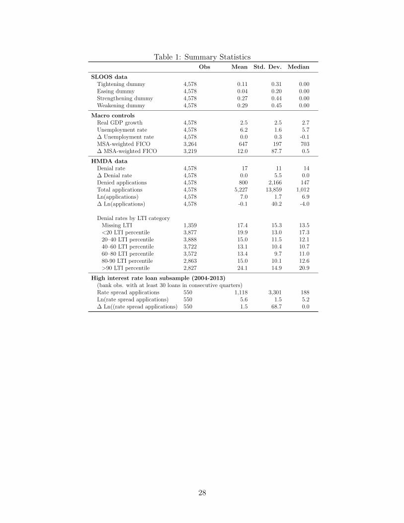
Table 1: Summary StatisticsObs Mean Std. Dev. Median
SLOOS dataTightening dummyEasing dummyStrengthening dummyWeakening dummy
4,5784,5784,5784,578
0.110.040.270.29
0.310.200.440.45
0.000.000.000.00
Macro controlsReal GDP growthUnemployment rate∆ Unemployment rateMSA-weighted FICO∆ MSA-weighted FICO
4,5784,5784,5783,2643,219
2.56.20.0647
12.0
2.51.60.3197
87.7
2.75.7
-0.17030.5
HMDA dataDenial rate∆ Denial rateDenied applicationsTotal applicationsLn(applications)∆ Ln(applications)
Denial rates by LTI categoryMissing LTI<20 LTI percentile20–40 LTI percentile40–60 LTI percentile60–80 LTI percentile80-90 LTI percentile>90 LTI percentile
4,5784,5784,5784,5784,5784,578
1,3593,8773,8883,7223,5722,8632,827
170.0800
5,2277.0
-0.1
17.419.915.013.113.415.024.1
115.5
2,16613,859
1.740.2
15.313.011.510.49.7
10.114.9
140.0147
1,0126.9
-4.0
13.517.312.110.711.012.620.9
High interest rate loan subsample (2004-2013)(bank obs. with at least 30 loans in consecutive quarters)Rate spread applications 550 1,118Ln(rate spread applications) 550 5.6∆ Ln((rate spread applications) 550 1.5
3,3011.5
68.7
1885.20.0
28
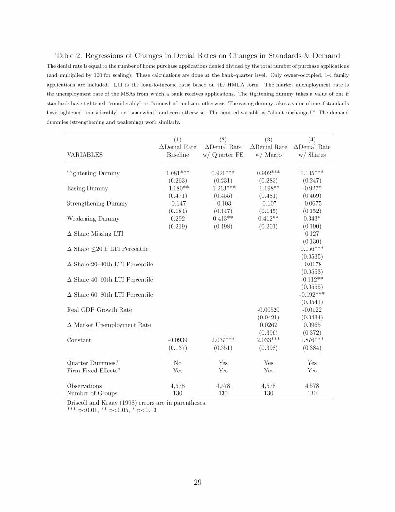
Table 2: Regressions of Changes in Denial Rates on Changes in Standards & DemandThe denial rate is equal to the number of home purchase applications denied divided by the total number of purchase applications
(and multiplied by 100 for scaling). These calculations are done at the bank-quarter level. Only owner-occupied, 1-4 family
applications are included. LTI is the loan-to-income ratio based on the HMDA form. The market unemployment rate is
the unemployment rate of the MSAs from which a bank receives applications. The tightening dummy takes a value of one if
standards have tightened “considerably” or “somewhat” and zero otherwise. The easing dummy takes a value of one if standards
have tightened “considerably” or “somewhat” and zero otherwise. The omitted variable is “about unchanged.” The demand
dummies (strengthening and weakening) work similarly.
VARIABLES
(1)∆Denial Rate
Baseline
(2)∆Denial Rate
w/ Quarter FE
(3)∆Denial Rate
w/ Macro
(4)∆Denial Rate
w/ Shares
Tightening Dummy
Easing Dummy
Strengthening Dummy
Weakening Dummy
∆ Share Missing LTI
∆ Share ≤20th LTI Percentile
∆ Share 20–40th LTI Percentile
∆ Share 40–60th LTI Percentile
∆ Share 60–80th LTI Percentile
Real GDP Growth Rate
∆ Market Unemployment Rate
Constant
Quarter Dummies?Firm Fixed Effects?
ObservationsNumber of Groups
1.081***(0.263)-1.180**(0.471)-0.147(0.184)0.292
(0.219)
-0.0939(0.137)
NoYes
4,578130
0.921***(0.231)
-1.203***(0.455)-0.103(0.147)0.413**(0.198)
2.037***(0.351)
YesYes
4,578130
0.902***(0.283)-1.198**(0.481)-0.107(0.145)0.412**(0.201)
-0.00520(0.0421)0.0262(0.396)
2.033***(0.398)
YesYes
4,578130
1.105***(0.247)-0.927*(0.469)-0.0675(0.152)0.343*(0.190)0.127
(0.130)0.156***(0.0535)-0.0178(0.0553)-0.112**(0.0555)-0.192***(0.0541)-0.0122(0.0434)0.0965(0.372)
1.876***(0.384)
YesYes
4,578130
Driscoll and Kraay (1998) errors are in parentheses.*** p<0.01, ** p<0.05, * p<0.10
29
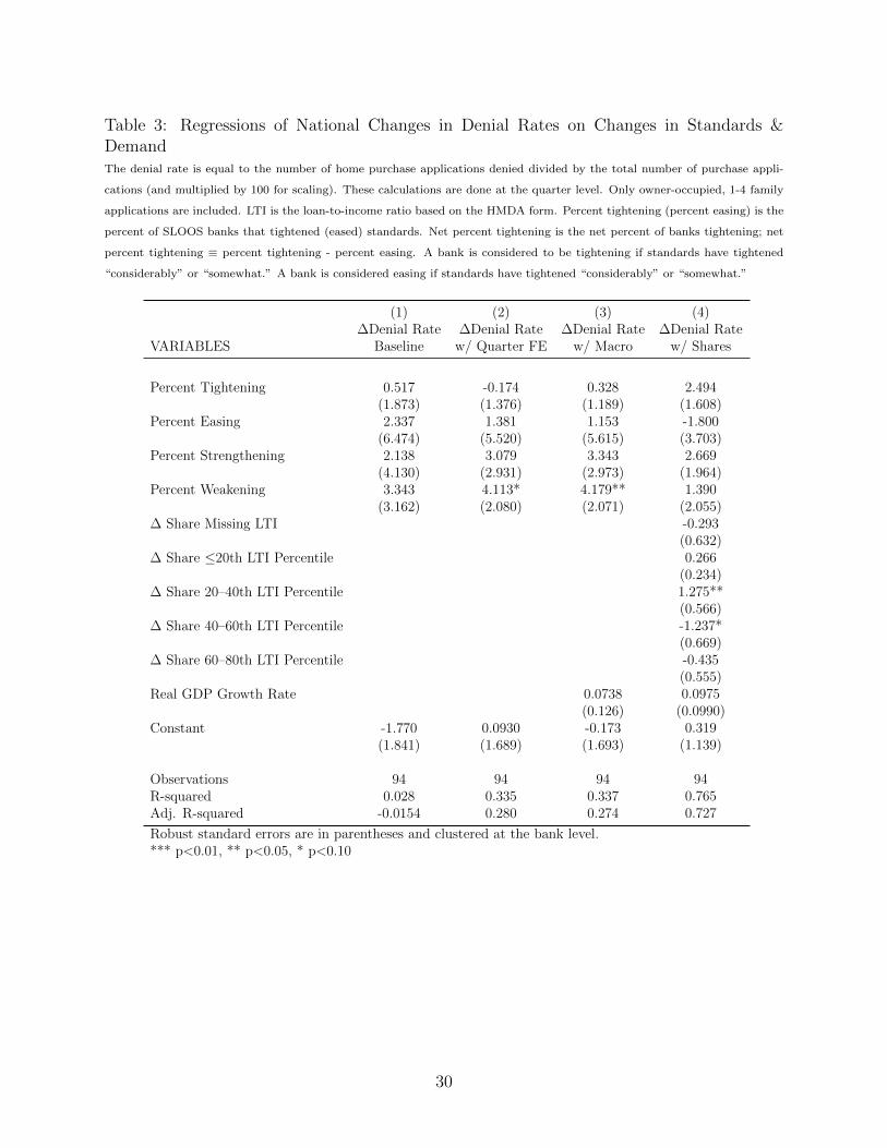
Table 3: Regressions of National Changes in Denial Rates on Changes in Standards &DemandThe denial rate is equal to the number of home purchase applications denied divided by the total number of purchase appli-
cations (and multiplied by 100 for scaling). These calculations are done at the quarter level. Only owner-occupied, 1-4 family
applications are included. LTI is the loan-to-income ratio based on the HMDA form. Percent tightening (percent easing) is the
percent of SLOOS banks that tightened (eased) standards. Net percent tightening is the net percent of banks tightening; net
percent tightening ≡ percent tightening - percent easing. A bank is considered to be tightening if standards have tightened
“considerably” or “somewhat.” A bank is considered easing if standards have tightened “considerably” or “somewhat.”
VARIABLES
(1)∆Denial Rate
Baseline
(2)∆Denial Rate
w/ Quarter FE
(3)∆Denial Rate
w/ Macro
(4)∆Denial Rate
w/ Shares
Percent Tightening
Percent Easing
Percent Strengthening
Percent Weakening
∆ Share Missing LTI
∆ Share ≤20th LTI Percentile
∆ Share 20–40th LTI Percentile
∆ Share 40–60th LTI Percentile
∆ Share 60–80th LTI Percentile
Real GDP Growth Rate
Constant
ObservationsR-squaredAdj. R-squared
0.517(1.873)2.337
(6.474)2.138
(4.130)3.343
(3.162)
-1.770(1.841)
940.028
-0.0154
-0.174(1.376)1.381
(5.520)3.079
(2.931)4.113*(2.080)
0.0930(1.689)
940.3350.280
0.328(1.189)1.153
(5.615)3.343
(2.973)4.179**(2.071)
0.0738(0.126)-0.173(1.693)
940.3370.274
2.494(1.608)-1.800(3.703)2.669
(1.964)1.390
(2.055)-0.293(0.632)0.266
(0.234)1.275**(0.566)-1.237*(0.669)-0.435(0.555)0.0975
(0.0990)0.319
(1.139)
940.7650.727
Robust standard errors are in parentheses and clustered at the bank level.*** p<0.01, ** p<0.05, * p<0.10
30
Table 4: Effects of Standards Changes Conditional on SecuritizationThe denial rate is equal to the number of home purchase applications denied divided by the total number of purchase applications
(and multiplied by 100 for scaling). These calculations are done at the bank-quarter level. Only owner-occupied, 1-4 family
applications are included. Securitizer = 1 for banks with 50 percent or more of their mortgages securitized in the last and
current quarter. Nonsecuritizers = 1 if securitizer = 0. LTI is the loan-to-income ratio based on the HMDA form. The market
unemployment rate is the unemployment rate of the MSAs from which a bank receives applications. The tightening dummy
takes a value of one if standards have tightened “considerably” or “somewhat” and zero otherwise. The easing dummy takes
a value of one if standards have tightened “considerably” or “somewhat” and zero otherwise. The omitted variable is “about
unchanged.” The demand dummies (strengthening and weakening) work similarly.
VARIABLES
(1)∆Denial Rate
Baseline
(2)∆Denial Rate
w/ Quarter FE & Macro
(3)∆Denial Rate
w/ Shares
Securitizer Dummy * Tightening Dummy
Securitizer Dummy * Easing Dummy
Nonsecuritizer Dummy * Tightening Dummy
Nonsecuritizer Dummy * Easing Dummy
Strengthening Dummy
Weakening Dummy
∆ Share Missing LTI
∆ Share ≤20th Percentile
∆ Share 20–40th Percentile
∆ Share 40–60th Percentile
∆ Share 60–80th Percentile
Real GDP Growth Rate
∆ Market Unemployment Rate
Constant
Quarter Dummies?Firm Fixed Effects?
F-Test Statistics From:F(1,92) test tight sec = tight nonsecF(1,92) test ease sec = ease nonsec
ObservationsNumber of Groups
0.111(0.307)-0.0604(0.589)
1.352***(0.353)-1.508**(0.603)-0.159(0.184)0.284
(0.219)
-0.0892(0.137)
NoYes
6.55*2.72
4,578130
0.304(0.240)0.279
(0.523)1.067***(0.369)
-1.627***(0.597)-0.122(0.144)0.408**(0.202)
-0.00484(0.0424)0.0349(0.395)
2.034***(0.397)
YesYes
3.12*5.83**
4,578130
0.472*(0.273)0.219
(0.476)1.279***(0.330)-1.261**(0.586)-0.0797(0.151)0.338*(0.191)0.128
(0.130)0.154***(0.0534)-0.0178(0.0551)-0.114**(0.0553)
-0.193***(0.0540)-0.0120(0.0437)
0.104(0.372)
1.876***(0.383)
YesYes
3.09*4.04**
4,578130
Driscoll and Kraay (1998) errors are in parentheses.*** p<0.01, ** p<0.05, * p<0.10
31
Tab
le5:
Reg
ress
ions
ofC
han
ges
inD
enia
lR
ates
onC
han
ges
inSta
ndar
ds
&D
eman
d,
by
LT
IC
ateg
ory
Th
ese et
ten
ed
Th
e e
mark
vh
a
scalin
g). tigh
oth
erw
ise.
ust
Th
e
mev
ati
on
for form
.
ha
A zero
100
ob
serv
y HM
D
stan
dard
s
an
d
b
if
hat”
on
e
w
of
mu
ltip
lied th
eon
som
e
base
d
ban
k-q
uart
er
alu
e “ h
(an
d
rati
o v or
eac
ay
“co
nsi
der
ab
ly” ,
cate
gory
ap
plica
tion
s
tak
TI
L
hase loan
-to-i
nco
me es
du
mm
the
ten
ing
ten
ed
hea
c
pu
rc
s Fi tigh or
of
TI
tigh
.
evLer
sim
ilarl
y
incl
ud
ed. h
a
b Th
e
um
n
ork
tota
l
w
are
ap
plica
tion
s.
stan
dard
s
the if
y
ap
plica
tion
s
on
e
enin
g)
b esei
v
f
div
ided
o eak
rec
alu
e w
fam
ily
ban
k v an
d
den
ied a
es
a
tak
1-4 h
wh
ic y
(str
ength
enin
g
qu
art
er.
ap
plica
tion
s
ccu
pie
d,
du
mm
from
pri
or
easi
ng
hase
wn
er-o
o
MS
As
du
mm
ies
the
Th
e
an
d
pu
rc
On
ly the
of
el.
rate
lev
of oth
erw
ise.
dem
an
d
hom
e
qu
art
er
Th
e
t
erb
ban
k-q
uart
er
ym
ent
zero
curr
en
um
n han
ged
.”
the in
to
un
emp
lo
an
d
the
un
c
oth
the
the
at
is
don
e
rate “
som
ewh
at”
ou
t
b
equ
al
“ab
isis or
rate
are t
calc
ula
tion
s enm
ap
plica
tion
s
den
ial
Th
e
un
emp
loy
“co
nsi
der
ab
ly”
vari
ab
le
30
om
itte
d
least
at
(1)
(2)
(3)
(4)
(5)
(6)
∆D
enia
lR
ate
∆D
enia
lR
ate
∆D
enia
lR
ate
∆D
enia
lR
ate
∆D
enia
lR
ate
∆D
enia
lR
ate
LT
ILT
ILT
ILT
ILT
ILT
IV
AR
IAB
LE
S≤
2020
-40
40-6
060
-80
80-9
0>
90
Tig
hte
nin
gD
um
my
0.63
0*1.
209*
**0.
826*
*0.
908*
*1.
192*
**1.
018*
*(0
.365
)(0
.426
)(0
.359
)(0
.373
)(0
.406
)(0
.416
)E
asin
gD
um
my
-0.9
17**
-1.6
90**
-1.2
24*
-1.3
07*
-2.0
43**
-1.5
68*
(0.4
41)
(0.7
27)
(0.6
84)
(0.6
63)
(0.8
23)
(0.8
82)
Str
engt
hen
ing
Du
mm
y-0
.041
7-0
.162
-0.2
150.
0763
-0.1
790.
0426
(0.2
15)
(0.1
91)
(0.2
33)
(0.2
10)
(0.2
82)
(0.2
95)
Wea
ken
ing
Du
mm
y0.
711*
*0.
0532
0.18
20.
357*
0.36
00.
628*
**(0
.322
)(0
.230
)(0
.240
)(0
.198
)(0
.258
)(0
.229
)R
eal
GD
PG
row
thR
ate
-0.0
894*
*-0
.002
030.
0048
20.
0179
0.01
190.
0086
7(0
.037
5)(0
.048
1)(0
.050
1)(0
.051
8)(0
.066
0)(0
.061
9)∆
Mar
ket
Un
emp
loym
ent
Rat
e0.
290
-0.2
700.
0214
-0.2
04-0
.519
-0.5
31(0
.251
)(0
.338
)(0
.469
)(0
.554
)(0
.534
)(0
.741
)C
onst
ant
2.58
4***
2.43
7***
1.41
7***
1.34
5***
1.39
6***
1.22
8**
(0.4
41)
(0.4
20)
(0.4
18)
(0.4
52)
(0.4
04)
(0.5
79)
Qu
arte
rD
um
mie
s?Y
esY
esY
esY
esY
esY
esF
irm
Fix
edE
ffec
ts?
Yes
Yes
Yes
Yes
Yes
Yes
Ob
serv
atio
ns
3,87
73,
888
3,72
23,
572
2,86
32,
827
Nu
mb
erof
Gro
ups
120
119
118
116
102
106
Dri
scol
lan
dK
raay
(199
8)er
rors
are
inp
aren
thes
es.
***
p<
0.01
,**
p<
0.05
,*
p<
0.10
32
Table 6: Regressions of Changes in Rate Spread Loans on Changes in Standards & DemandThe change in home purchase loans is measured in log differences (and multiplied by 100 for scaling). These calculations
are done at the bank-quarter level. Only owner-occupied, 1-4 family applications are included. Rate spread is a definition
set by HMDA and is only defined for approved loans. Only bank observations that have 30 or more rate spread loans in
consecutive quarters are included. LTI is the loan-to-income ratio based on the HMDA form. The market unemployment
rate is the unemployment rate of the MSAs from which a bank receives applications. The tightening dummy takes a value of
one if standards have tightened “considerably” or “somewhat” and zero otherwise. The easing dummy takes a value of one if
standards have tightened “considerably” or “somewhat” and zero otherwise. The omitted variable is “about unchanged.” The
demand dummies (strengthening and weakening) work similarly.
VARIABLES
(1)Log Diff Apps
Baseline
(2)Log Diff Appsw/ Quarter FE
(3)Log Diff Apps
w/ Macro
(4)Log Diff Apps
w/ Shares
Tightening Dummy
Easing Dummy
Strengthening Dummy
Weakening Dummy
∆ Share Missing LTI
∆ Share ≤20th LTI Percentile
∆ Share 20–40th LTI Percentile
∆ Share 40–60th LTI Percentile
∆ Share 60–80th LTI Percentile
Real GDP Growth Rate
∆ Market Unemployment Rate
Constant
Quarter Dummies?Firm Fixed Effects?
ObservationsR-squaredAdj. R-squared
-18.55***(5.046)31.10
(22.06)2.340
(10.89)5.004
(7.525)
2.135(4.973)
NoYes
5500.074-0.017
-19.90***(5.387)29.24
(21.76)0.667
(11.16)5.234
(7.881)
8.729(7.453)
YesYes
5500.089-0.007
-14.27***(5.125)26.37
(21.79)3.126
(11.41)5.679
(8.127)
1.125(1.346)-11.02*(6.442)13.56*(7.802)
YesYes
5500.0990.000
-16.24**(6.946)18.91
(16.88)-1.125(11.66)0.175
(8.469)6.515*(3.621)-1.034(3.597)1.349
(3.001)2.048
(3.693)6.074
(4.461)0.629
(1.141)-13.46**(6.606)14.43
(8.903)
YesYes
5500.1450.043
Robust standard errors are in parentheses and clustered at the bank level.*** p<0.01, ** p<0.05, * p<0.10
33
Table 7: Regressions of Changes in Credit Approved on Changes in Standards & DemandCredit is the total dollar amount of home purchase loans approved. Changes in credit is measured in log differences (and
multiplied by 100 for scaling). These calculations are done at the bank-quarter level. Only owner-occupied, 1-4 family applica-
tions are included. Income percentile thresholds are based on HMDA data and set each quarter. The market unemployment
rate is the unemployment rate of the MSAs from which a bank receives applications. The tightening dummy takes a value of
one if standards have tightened “considerably” or “somewhat” and zero otherwise. The easing dummy takes a value of one if
standards have tightened “considerably” or “somewhat” and zero otherwise. The omitted variable is “about unchanged.” The
demand dummies (strengthening and weakening) work similarly.
VARIABLES
(1)Log Diff Credit
Baseline
(2)Log Diff Credit
w/ Macro & Quarter FE
(3)Log Diff Credit
w/ Income
Tightening Dummy
Easing Dummy
Strengthening Dummy
Weakening Dummy
∆ Share Income Missing
∆ Share Income Percentile <10
∆ Share Income Percentile 10–25
∆ Share Income Percentile 25-50
∆ Share Income Percentile 50–75
∆ Share Income Percentile 75–90
Real GDP Growth Rate
∆ Market Unemployment Rate
Constant
Quarter Dummies?Firm Fixed Effects?
ObservationsNumber of Groups
-8.645***(2.675)8.294*(4.842)
7.742***(1.967)-1.797(2.356)
-0.179(1.073)
NoYes
4,578130
-4.472**(2.036)5.979
(4.452)4.176***(1.272)-2.169(1.642)
0.257(0.266)
-5.653***(1.835)
-8.081***(2.860)
YesYes
4,578130
-5.010**(2.232)5.376
(4.645)4.050***(1.197)-2.439(1.680)0.158
(0.624)-1.210***(0.370)-0.383(0.352)0.338
(0.479)0.968*(0.577)0.289
(0.356)0.153
(0.305)-6.301***(2.078)
-8.667***(3.202)
YesYes
4,578130
Driscoll and Kraay (1998) errors are in parentheses.*** p<0.01, ** p<0.05, * p<0.10
34

Table 8: Regressions of Changes in Applications on Changes in Standards & DemandThe change in home purchase loans is measured in log differences (and multiplied by 100 for scaling). These calculations are
done at the bank-quarter level. Only owner-occupied, 1-4 family applications are included. The market unemployment rate is
the unemployment rate of the MSAs from which a bank receives applications. The tightening dummy takes a value of one if
standards have tightened “considerably” or “somewhat” and zero otherwise. The easing dummy takes a value of one if standards
have tightened “considerably” or “somewhat” and zero otherwise. The omitted variable is “about unchanged.” The demand
dummies (strengthening and weakening) work similarly.
VARIABLES
(1)Log Diff Apps
Baseline
(2)Log Diff Appsw/ Quarter FE
(3)Log Diff Apps
w/ Macro
Tightening Dummy
Easing Dummy
Strengthening Dummy
Weakening Dummy
Real GDP Growth Rate
∆ Market Unemployment Rate
Constant
Quarter Dummies?Firm Fixed Effects?
ObservationsNumber of Groups
-5.588**(2.273)3.333
(3.856)7.794***(1.709)-1.454(2.011)
-1.296(0.921)
NoYes
4,578130
-3.869*(2.029)1.866
(3.572)4.039***(1.237)-1.725(1.346)
-10.22***(2.114)
YesYes
4,578130
-1.570(2.034)1.140
(3.506)4.525***(1.283)-1.742(1.327)0.327
(0.239)-5.244***(1.669)
-8.080***(2.782)
YesYes
4,578130
Driscoll and Kraay (1998) errors are in parentheses.*** p<0.01, ** p<0.05, * p<0.10
35
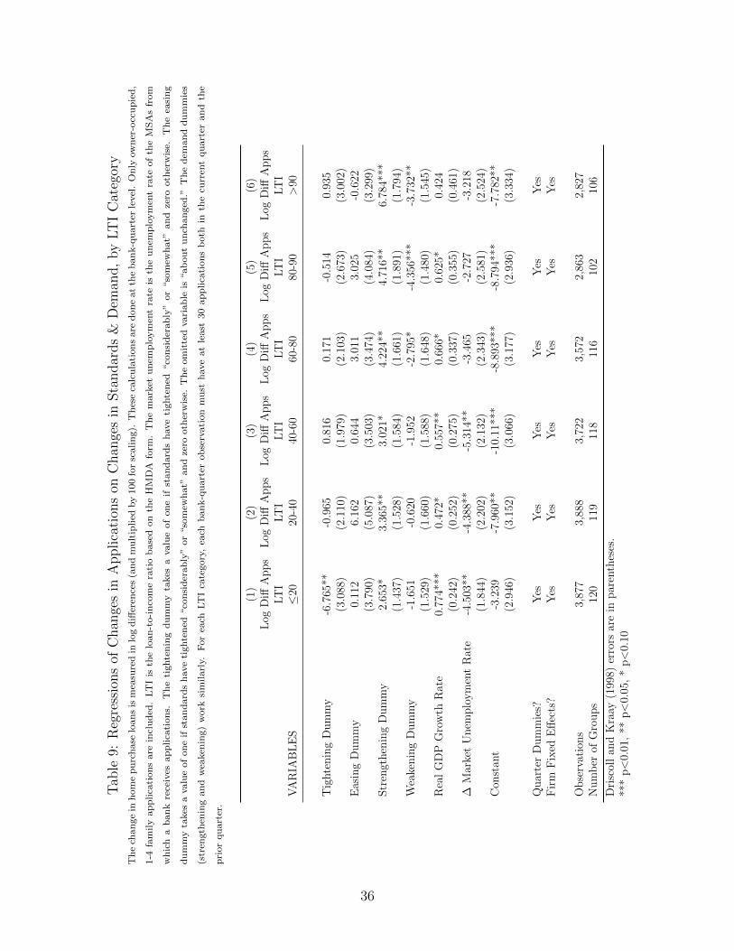
Tab
le9:
Reg
ress
ions
ofC
han
ges
inA
pplica
tion
son
Chan
ges
inSta
ndar
ds
&D
eman
d,
by
LT
IC
ateg
ory
ccu
pie
d,
from
easi
ng
du
mm
ies
the
MS
As
an
d
Th
e
ow
ner
-o
the
of dem
an
d
qu
art
er
On
ly
rate
oth
erw
ise.
t
Th
e
el.
t curr
en
lev
ym
en zero e
th
ban
k-q
uart
er
un
emp
lo an
d
han
ged
.”
in
“so
mew
hat” un
c
oth
b
ou
t
the
“ab
the
is is
at
rate or
ap
plica
tion
s
don
e
ym
ent
“co
nsi
der
ab
ly”
30
vari
ab
le
are
least
calc
ula
tion
s
un
emp
lo
om
itte
d
at
ev
ha
et Th
e
ten
ed
mark ust
Th
ese
tigh m
Th
e
ev ati
on
scalin
g).
ha oth
erw
ise.
form
.
stan
dard
s
zero
an
d
bse
rvo
for A r
HM
D te
100
if
yb the
on
e
ult
iplied
on
of
“so
mew
hat”
ban
k-q
uar
m base
d h
alu
e
or
eac
v ,
nd
(a rati
o aes
diff
eren
ces
tak
cate
gory
y
“co
nsi
der
ab
ly”
TI
du
mm L
hea
c
log
in loan
-to-i
nco
me
ten
ed
ten
ing
or
tigh F
mea
sure
d the
tigh e
vh
a
TI
L Th
e
sim
ilarl
y.
is
is
stan
dard
s
incl
ud
ed.
ap
plica
tion
s. ork
loan
s
w
hase
if
are on
e
enin
g)
pu
rc of
esre
ceiv
alu
e w
hom
ein ap
plica
tion
s eak
v an
d
a
ban
k es
han
ge
y tak
c fam
il a y
h
Th
e
1-4
wh
ic
du
mm
(str
ength
enin
g
qu
art
er.
pri
or
(1)
(2)
(3)
(4)
(5)
(6)
Log
Diff
Apps
Log
Diff
Apps
Log
Diff
Apps
Log
Diff
Apps
Log
Diff
Apps
Log
Diff
Apps
LT
ILT
ILT
ILT
ILT
ILT
IV
AR
IAB
LE
S≤
2020
-40
40-6
060
-80
80-9
0>
90
Tig
hte
nin
gD
um
my
-6.7
65**
-0.9
650.
816
0.17
1-0
.514
0.93
5(3
.088
)(2
.110
)(1
.979
)(2
.103
)(2
.673
)(3
.002
)E
asin
gD
um
my
0.11
26.
162
0.64
43.
011
3.02
5-0
.622
(3.7
90)
(5.0
87)
(3.5
03)
(3.4
74)
(4.0
84)
(3.2
99)
Str
engt
hen
ing
Dum
my
2.65
3*3.
365*
*3.
021*
4.22
4**
4.71
6**
6.78
4***
(1.4
37)
(1.5
28)
(1.5
84)
(1.6
61)
(1.8
91)
(1.7
94)
Wea
kenin
gD
um
my
-1.6
51-0
.620
-1.9
52-2
.795
*-4
.356
***
-3.7
32**
(1.5
29)
(1.6
60)
(1.5
88)
(1.6
48)
(1.4
80)
(1.5
45)
Rea
lG
DP
Gro
wth
Rat
e0.
774*
**0.
472*
0.55
7**
0.66
6*0.
625*
0.42
4(0
.242
)(0
.252
)(0
.275
)(0
.337
)(0
.355
)(0
.461
)∆
Mar
ket
Unem
plo
ym
ent
Rat
e-4
.503
**-4
.388
**-5
.314
**-3
.465
-2.7
27-3
.218
(1.8
44)
(2.2
02)
(2.1
32)
(2.3
43)
(2.5
81)
(2.5
24)
Con
stan
t-3
.239
-7.9
60**
-10.
11**
*-8
.893
***
-8.7
94**
*-7
.782
**(2
.946
)(3
.152
)(3
.066
)(3
.177
)(2
.936
)(3
.334
)
Quar
ter
Dum
mie
s?Y
esY
esY
esY
esY
esY
esF
irm
Fix
edE
ffec
ts?
Yes
Yes
Yes
Yes
Yes
Yes
Obse
rvat
ions
3,87
73,
888
3,72
23,
572
2,86
32,
827
Num
ber
ofG
roups
120
119
118
116
102
106
Dri
scol
lan
dK
raay
(199
8)er
rors
are
inpar
enth
eses
.**
*p<
0.01
,**
p<
0.05
,*
p<
0.10
36
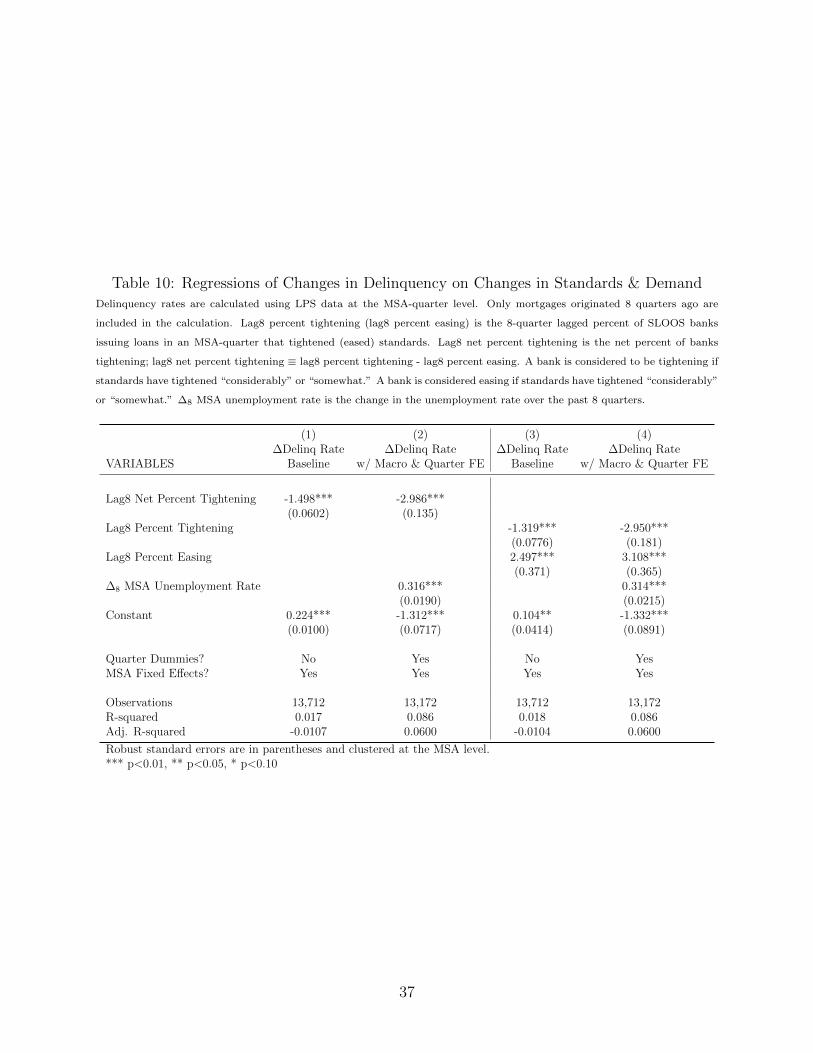
Table 10: Regressions of Changes in Delinquency on Changes in Standards & DemandDelinquency rates are calculated using LPS data at the MSA-quarter level. Only mortgages originated 8 quarters ago are
included in the calculation. Lag8 percent tightening (lag8 percent easing) is the 8-quarter lagged percent of SLOOS banks
issuing loans in an MSA-quarter that tightened (eased) standards. Lag8 net percent tightening is the net percent of banks
tightening; lag8 net percent tightening ≡ lag8 percent tightening - lag8 percent easing. A bank is considered to be tightening if
standards have tightened “considerably” or “somewhat.” A bank is considered easing if standards have tightened “considerably”
or “somewhat.” ∆8 MSA unemployment rate is the change in the unemployment rate over the past 8 quarters.
(1) (2) (3) (4)∆Delinq Rate ∆Delinq Rate ∆Delinq Rate ∆Delinq Rate
VARIABLES Baseline w/ Macro & Quarter FE Baseline w/ Macro & Quarter FE
Lag8 Net Percent Tightening -1.498*** -2.986***(0.0602) (0.135)
Lag8 Percent Tightening -1.319*** -2.950***(0.0776) (0.181)
Lag8 Percent Easing 2.497*** 3.108***(0.371) (0.365)
∆8 MSA Unemployment Rate 0.316*** 0.314***(0.0190) (0.0215)
Constant 0.224*** -1.312*** 0.104** -1.332***(0.0100) (0.0717) (0.0414) (0.0891)
Quarter Dummies? No Yes No YesMSA Fixed Effects? Yes Yes Yes Yes
Observations 13,712 13,172 13,712 13,172R-squared 0.017 0.086 0.018 0.086Adj. R-squared -0.0107 0.0600 -0.0104 0.0600
Robust standard errors are in parentheses and clustered at the MSA level.*** p<0.01, ** p<0.05, * p<0.10
37
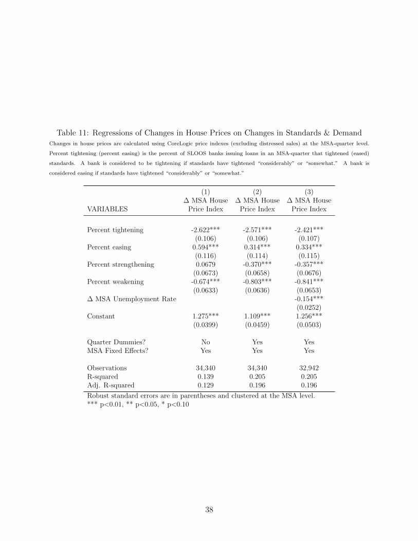
Table 11: Regressions of Changes in House Prices on Changes in Standards & DemandChanges in house prices are calculated using CoreLogic price indexes (excluding distressed sales) at the MSA-quarter level.
Percent tightening (percent easing) is the percent of SLOOS banks issuing loans in an MSA-quarter that tightened (eased)
standards. A bank is considered to be tightening if standards have tightened “considerably” or “somewhat.” A bank is
considered easing if standards have tightened “considerably” or “somewhat.”
VARIABLES
(1)∆ MSA House
Price Index
(2)∆ MSA House
Price Index
(3)∆ MSA House
Price Index
Percent tightening
Percent easing
Percent strengthening
Percent weakening
∆ MSA Unemployment Rate
Constant
Quarter Dummies?MSA Fixed Effects?
ObservationsR-squaredAdj. R-squared
-2.622***(0.106)
0.594***(0.116)0.0679
(0.0673)-0.674***(0.0633)
1.275***(0.0399)
NoYes
34,3400.1390.129
-2.571***(0.106)
0.314***(0.114)
-0.370***(0.0658)-0.803***(0.0636)
1.109***(0.0459)
YesYes
34,3400.2050.196
-2.421***(0.107)
0.334***(0.115)
-0.357***(0.0676)-0.841***(0.0653)
-0.154***(0.0252)1.256***(0.0503)
YesYes
32,9420.2050.196
Robust standard errors are in parentheses and clustered at the MSA level.*** p<0.01, ** p<0.05, * p<0.10
38

-100
-80
-60
-40
-20
0
20
40
60
80
100Percent
1991 1993 1995 1997 1999 2001 2003 2005 2007 2009 2011 2013-100
-80
-60
-40
-20
0
20
40
60
80
100Percent
1991 1993 1995 1997 1999 2001 2003 2005 2007 2009 2011 2013
Eas
ing
T
ight
enin
g
Quarterly
Reported Changes in Standards for Residential Real Estate Loans
-100
-80
-60
-40
-20
0
20
40
60
80
100Percent
1991 1993 1995 1997 1999 2001 2003 2005 2007 2009 2011 2013-100
-80
-60
-40
-20
0
20
40
60
80
100Percent
1991 1993 1995 1997 1999 2001 2003 2005 2007 2009 2011 2013
W
eake
ning
Str
engt
heni
ng
Quarterly
Reported Changes in Demand for Residential Real Estate Loans
Note: The question on changes in demand for RRE loans was not asked in 1990:Q2 and 1991:Q2. Shaded bars indicate periods of business recession as defined by the National Bureau of Economic Research. Source: SLOOS.
Figure 1: Standards and Demand, 1990–2013
39
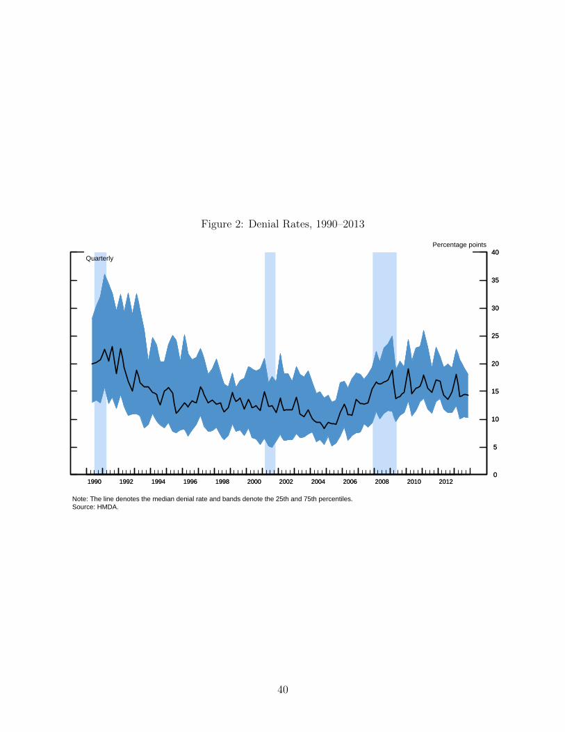
1990 1992 1994 1996 1998 2000 2002 2004 2006 2008 2010 2012 0
5
10
15
20
25
30
35
40Percentage points
Note: The line denotes the median denial rate and bands denote the 25th and 75th percentiles. Source: HMDA.
1990 1992 1994 1996 1998 2000 2002 2004 2006 2008 2010 2012 0
5
10
15
20
25
30
35
40Quarterly
Figure 2: Denial Rates, 1990–2013
40
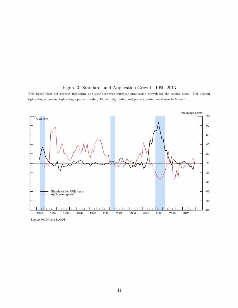
Figure 3: Standards and Application Growth, 1990–2013This figure plots net percent tightening and year-over-year purchase application growth for the testing panel. Net percent
tightening ≡ percent tightening - percent easing. Percent tightening and percent easing are shown in figure 1.
Source: HMDA and SLOOS.
1990 1992 1994 1996 1998 2000 2002 2004 2006 2008 2010 2012-100
-80
-60
-40
-20
0
20
40
60
80
100Percentage points
Standards for RRE loansApplication growth
Quarterly
41