The RD53A Pixel Readout Chip - indico.physics.lbl.gov€¦ · Pixel Size 50x250 µm2 50x50 µm2...
51
UNIVERSITY OF CALIFORNIA The RD53A Pixel Readout Chip Instrumentation Brownbag 08/16/17 1 Timon Heim - LBNL
Transcript of The RD53A Pixel Readout Chip - indico.physics.lbl.gov€¦ · Pixel Size 50x250 µm2 50x50 µm2...

UNIVERSITY OF CALIFORNIA
The RD53A Pixel Readout Chip
Instrumentation Brownbag08/16/17
1
Timon Heim - LBNL
Timon Heim 2 Instrumentation Seminar
Outline• ATLAS experiment and its Phase-2 upgrade in a nutshell
• RD53 collaboration and LBNL contribution
• Radiation tolerance of 65nm technology
• The RD53A demonstrator
• Overview
• Analog front-ends and results from test chips
• Digital architecture
• *New* features
• Preparations for testing
• Conclusion and Outlook

Timon Heim 3 Instrumentation Seminar
ATLAS Experiment

Timon Heim 4 Instrumentation Seminar
ATLAS Pixel Detector
Hybrid Technology:• Dedicated sensor and readout chip,
connected via bump bond• Mixed signal readout chip with per pixel
amplifier and discriminator• Two main sensor technologies:
• Planar• 3D

Timon Heim 5 Instrumentation Seminar
Pixel Readout Chip at the LHCRequirements:
• Collisions occur every 25ns• Convert charge to digital value,
typically Time-over-Threshold in 25ns units
• Store charge and time of each hit locally for a some µs (trigger latency)
• Read out hits which have been triggered, bandwidth > trigger frequency * number of hits
DAC Global Threshold
Hit OutAmp
Bias
ThresholdRegister
LHC → Summer Rain HL-LHC → Pouring Storm
• Store full time sequence of drops until trigger (not collect in a bucket) → more memory• High resolution to distinguish between drops → smaller pixels• Drops damage sensor and readout chip → higher radiation tolerance

Timon Heim 6 Instrumentation Seminar
Timeline
2011 2012 2013 2014 2015 2016 2017 2018 2019 2020 2021 2022 2023 2024 2025 2035
Phase 0 Upgrade
Phase 1 Upgrade
Phase 2 Upgrade
LS1 LS2 LS3
75% nominalluminosity
7/8 TeVnominal
luminosity
13/14 TeV2 x nominal luminosity
14 TeV5 to 7 x nominal
luminosity
14 TeV
30 fb-1 150 fb-1 300 fb-1 3000 fb-1
We are here
Run 1 Run 2 Run 3 HL-LHC
….
Current Tracker Readout
ITkChip Size 2x2cm2 2x2 cm2
Pixel Size 50x250 µm2 50x50 µm2
Pixel Hit Rate 400 MHz/cm2 3 GHz/cm2
Trigger rate 200 kHz 1 MHzTrigger Latency 6.4 µs 12.8 µs
Current consumption 20 µA/pixel <8 µA/pixelRadiation Tolerance 300 Mrad 0.5-1 Grad
Min. stable Threshold 1500 e 600 e
ATLAS Phase 2 Upgrade will replace Inner detector with new all-silicon tracker, the Inner Tracker (ITk)

Timon Heim 7 Instrumentation Seminar
RD53 CollaborationOverview:• R&D program aiming to develop
pixel readout chips in 65nm technology
• Consisting of ATLAS and CMS groups
Goals:• Study of radiation effects in 65nm• Develop design flow to efficiently
design large pixel readout chips• Design of shared rad-hard IPs• Design and test a large scale
65nm pixel readout chip → RD53A

Timon Heim 8 Instrumentation Seminar
LBNL Contributions
LBNL ATLAS Group:• FE65P2:
• Verification: Rebecca• Testing: Ben, Katie, Rebecca, Maurice, Timon,
Veronica• DAQ: Timon
• RD53A:• Verification: Cesar• Preparation for testing: Aleksandra, Katie,
Adrien, Maurice, Timon• DAQ: Arnaud, Timon• Cable testing: Veronica
Great internal collaboration with IC design group and external collaboration with Universities!
LBNL IC design group:• Abder: Initial analog front-end
design, FE65P2• Dario: analog front-end design,
FE65P2, DRAD, RD53A• Amanda: RD53A analog front-end
design
Visitors:• FE65P2:
• Testing: Lashkar• RD53A:
• DAQ: Nikola, Lev• Wafer probing: Xiangyang

Timon Heim 9 Instrumentation Seminar
Radiation Hardness
Take-away points:• Total Ionising Dose (TID) effects can
damage CMOS transistors• 65nm is intrinsically very radiation hard
More details in Instrumentation Colloquium:“Radiation Effects in CMOS Technologies for LHC Detector Upgrades”
by Federico Faccio
• Analog: avoid narrow & short transistors• Digital: qualified 9T std library in
dedicated test chip

Timon Heim 10 Instrumentation Seminar
RD53A Overview400 pixels / 20 mm
192
pixe
ls /
11.8
mm Synchronous
Analog Front-EndLinear
Analog Front-EndDifferential
Analog Front-End
Periphery
76,800 x 50x50µm2 pixels

Timon Heim 11 Instrumentation Seminar
RD53A Specs

Timon Heim 12 Instrumentation Seminar
Analog Islands & Digital Sea
Design strategy:• All analog FE flavours fit into
the same 35x35µm2 area• Analog FEs are arranged in
2x2 analog islands• Digital on-top• Digital logic can be
synthesised around the analog islands → No step-and-repeat design
• Hierarchical design to enable fast verification
50µm
35µm
Analog 2x2-pixel Island
SynthesisedDigital Sea
Bump pad

Timon Heim 13 Instrumentation Seminar
Digital Pixel Region
Centralised Buffer Architecture (CBA):• 4x4 pixel per region• Each region has 16 memories to store:
• 9-bit timestamp• 16-bit hit map• 6 x 4-bit ToT values
• P&R ~90-95% full
Distributed Buffer Architecture (CBA):• 4x1 pixel per region• Each pixel has 8 x 4-bit ToT memories• Each region has 8 x 9-bit Latency timer
memories• P&R ~80-85% full
One Pixel:

Timon Heim 14 Instrumentation Seminar
Digital Architecture
8x8 Digital Core
8x8 Digital Core
8x8 Digital Core
…
8x8 Digital Core
8x8 Digital Core
8x8 Digital Core
…
8x8 Digital Core
8x8 Digital Core
8x8 Digital Core
…
…
…
…
End of Column
Digital Core:• Small enough for
transistor level simulation
• Tiles of synthesised logic connected during place & route
• Two kinds of digital buffer architecture:• 4x4• 4x1
24x
50x

Timon Heim 15 Instrumentation Seminar
Analog Front-EndsRD53A
Chipix65:• 64x64 pixel• Submitted summer 2016• Synchronous and Linear
front-end• 4x4 Centralised buffer
architecture• 4x4 digital core• DAC, ADC, bandgap,
CERN I/O pads
Towards RD53A:• Two small scale prototypes:
• Exercise “analog island in digital sea” design flow
• Test analog front-end designs• Test vehicle for irradiations• 50x50µm2 sensor
development
FE65P2:• 64x64 pixel• Submitted fall 2015• Differential front-end• 2x2 distributed buffer
architecture• 4x64 digital core• Digital logic from FE-I4• Barebone periphery

Timon Heim 16 Instrumentation Seminar
Differential Front-End
Charge Sensitive Amplifier:• Straight cascode design• Global settings for If (8bit DAC)• No per pixel adjustment• Selectable gain
Two Stage Comparator:• Differential design• Global 8bit threshold DAC• Two per pixel 4bit threshold DACs• Optimised for low threshold operation
V
t
a
b cba c
Timon Heim 17 Instrumentation Seminar
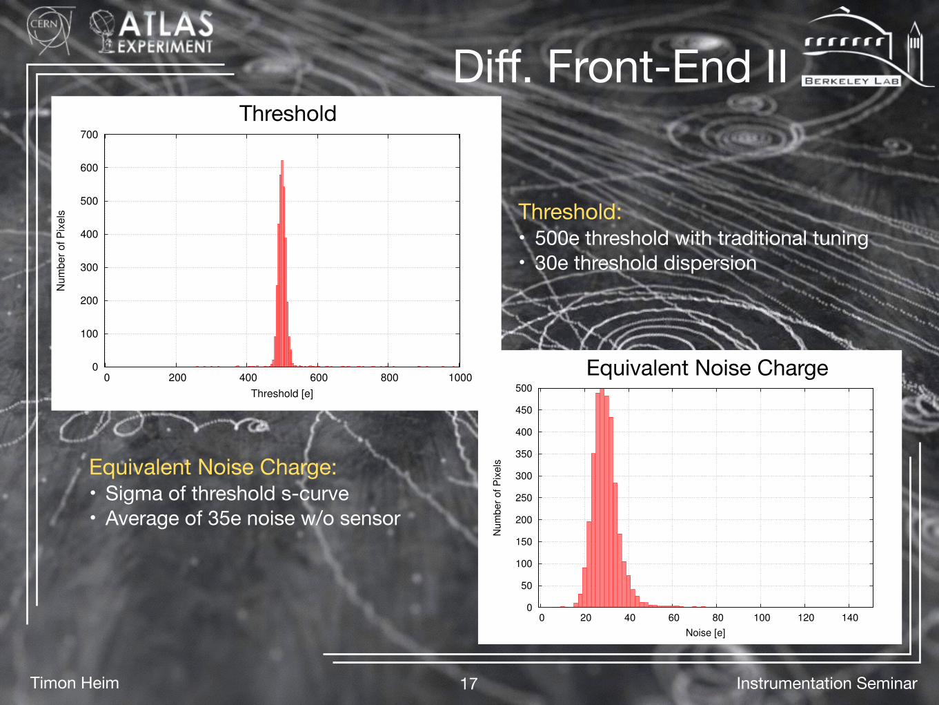
Diff. Front-End II
Threshold:• 500e threshold with traditional tuning• 30e threshold dispersion
0
100
200
300
400
500
600
700
0 200 400 600 800 1000
Num
ber
of P
ixels
Threshold [e]
ThresholdDist
0
50
100
150
200
250
300
350
400
450
500
0 20 40 60 80 100 120 140
Nu
mb
er
of
Pix
els
Noise [e]
NoiseDist
Equivalent Noise Charge:• Sigma of threshold s-curve• Average of 35e noise w/o sensor
Threshold
Equivalent Noise Charge
Timon Heim 18 Instrumentation Seminar
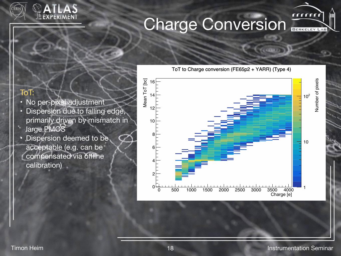
Charge Conversion
ToT:• No per-pixel adjustment• Dispersion due to falling edge,
primarily driven by mismatch in large PMOS
• Dispersion deemed to be acceptable (e.g. can be compensated via offline calibration)
Num
ber o
f pix
els
1
10
210
ToT to Charge conversion (FE65p2 + YARR) (Type 4)
Charge [e]0 500 1000 1500 2000 2500 3000 3500 4000
Mea
n To
T [b
c]
0
2
4
6
8
10
12
14
16
ToT to Charge conversion (FE65p2 + YARR) (Type 4)

Timon Heim 19 Instrumentation Seminar
FE65P2 IrradiationProton irradiation:• 800MeV protons at LANL• Irradiated total of 6 modules• Two chips for each TID: 150MRad,
350MRad, and 500MRad• Unfortunately one 500MRad chip
died of ESD before irrad., and the other was not centred in the beam
Noise [e]0 20 40 60 80 100 120 140
Num
ber o
f Pix
els
0
50
100
150
200
250
300
350
400
Noise [e] 0 20 40 60 80 100 120 140
Num
ber o
f Pix
els
0
50
100
150
200
250Noise [e]
0 20 40 60 80 100 120 140
Num
ber o
f Pix
els
0
50
100
150
200
250
before irradiation
150 MRad
350 MRad
Timon Heim 20 Instrumentation Seminar
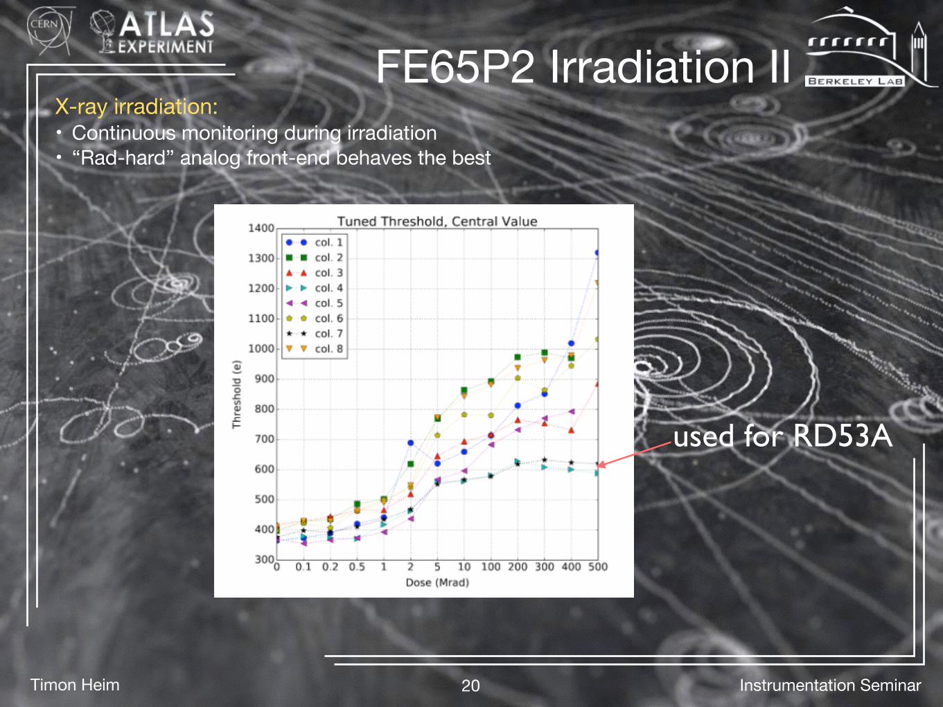
FE65P2 Irradiation IIX-ray irradiation:• Continuous monitoring during irradiation• “Rad-hard” analog front-end behaves the best
used for RD53A

Timon Heim 21 Instrumentation Seminar
Discriminator Speed
Trade-off: higher CompVbn = less
timing dispersion, but higher current consumption

Timon Heim 22 Instrumentation Seminar
FE65P2 Sensor Module
0
50
100
150
200
250
300
350
400
450
500
0 20 40 60 80 100 120 140
Num
ber
of P
ixels
Noise [e]
NoiseDist
0
100
200
300
400
500
600
700
0 200 400 600 800 1000
Num
ber
of P
ixels
Threshold [e]
ThresholdDist
pl0_residualXEntries 134801Mean -0.001853RMS 0.0141
-0.3 -0.2 -0.1 0 0.1 0.2 0.30
1000
2000
3000
4000
5000
6000
7000
pl0_residualXEntries 134801Mean -0.001853RMS 0.0141
pl0_residualXpl20_residualXEntries 120541Mean -0.001934RMS 0.07004
-0.3 -0.2 -0.1 0 0.1 0.2 0.30
100
200
300
400
500
600 pl20_residualXEntries 120541Mean -0.001934RMS 0.07004
pl20_residualXpl21_residualXEntries 105180Mean -0.01267RMS 0.0712
-0.3 -0.2 -0.1 0 0.1 0.2 0.30
100
200
300
400
500pl21_residualXEntries 105180Mean -0.01267RMS 0.0712
pl21_residualXpl1_residualXEntries 134801Mean 0.001707RMS 0.01147
-0.3 -0.2 -0.1 0 0.1 0.2 0.30
2000
4000
6000
8000
10000pl1_residualXEntries 134801Mean 0.001707RMS 0.01147
pl1_residualXpl30_residualXEntries 11442Mean -0.01498RMS 0.03938
-0.3 -0.2 -0.1 0 0.1 0.2 0.30
20
40
60
80
100
120
140
160
180
200
220
240pl30_residualXEntries 11442Mean -0.01498RMS 0.03938
pl30_residualXpl22_residualXEntries 102332Mean -0.02114RMS 0.07579
-0.3 -0.2 -0.1 0 0.1 0.2 0.30
50
100
150
200
250
300
350
400
450
pl22_residualXEntries 102332Mean -0.02114RMS 0.07579
pl22_residualX
pl0_residualYEntries 134801Mean 0.0002244RMS 0.01302
-0.3 -0.2 -0.1 0 0.1 0.2 0.30
1000
2000
3000
4000
5000
6000
7000
8000pl0_residualYEntries 134801Mean 0.0002244RMS 0.01302
pl0_residualYpl20_residualYEntries 120541Mean 0.001101RMS 0.01496
-0.3 -0.2 -0.1 0 0.1 0.2 0.30
500
1000
1500
2000
2500
3000
pl20_residualYEntries 120541Mean 0.001101RMS 0.01496
pl20_residualYpl21_residualYEntries 105180Mean 0.0003436RMS 0.01632
-0.3 -0.2 -0.1 0 0.1 0.2 0.30
500
1000
1500
2000
2500pl21_residualYEntries 105180Mean 0.0003436RMS 0.01632
pl21_residualYpl1_residualYEntries 134801Mean -9.942e-05RMS 0.01032
-0.3 -0.2 -0.1 0 0.1 0.2 0.30
2000
4000
6000
8000
10000
pl1_residualYEntries 134801Mean -9.942e-05RMS 0.01032
pl1_residualYpl30_residualYEntries 11442Mean -0.002RMS 0.02521
-0.3 -0.2 -0.1 0 0.1 0.2 0.30
50
100
150
200
250
pl30_residualYEntries 11442Mean -0.002RMS 0.02521
pl30_residualYpl22_residualYEntries 102332Mean -0.00249RMS 0.01981
-0.3 -0.2 -0.1 0 0.1 0.2 0.30
200
400
600
800
1000
1200
1400
1600
1800
2000
2200
pl22_residualYEntries 102332Mean -0.00249RMS 0.01981
pl22_residualY
pl23_residualXEntries 83996Mean -0.003974RMS 0.07124
-0.3 -0.2 -0.1 0 0.1 0.2 0.30
50
100
150
200
250
300
350
400pl23_residualXEntries 83996Mean -0.003974RMS 0.07124
pl23_residualXpl24_residualXEntries 103286Mean 0.01455RMS 0.07524
-0.3 -0.2 -0.1 0 0.1 0.2 0.30
50
100
150
200
250
300
350
400
450
pl24_residualXEntries 103286Mean 0.01455RMS 0.07524
pl24_residualXpl25_residualXEntries 79371Mean 0.0137RMS 0.08124
-0.3 -0.2 -0.1 0 0.1 0.2 0.30
50
100
150
200
250
300
350
pl25_residualXEntries 79371Mean 0.0137RMS 0.08124
pl25_residualXpl2_residualXEntries 134801Mean -0.001706RMS 0.01178
-0.3 -0.2 -0.1 0 0.1 0.2 0.30
1000
2000
3000
4000
5000
6000
7000
8000
pl2_residualXEntries 134801Mean -0.001706RMS 0.01178
pl2_residualXpl3_residualXEntries 134801Mean 0.0006579RMS 0.006384
-0.3 -0.2 -0.1 0 0.1 0.2 0.30
2000
4000
6000
8000
10000
12000pl3_residualXEntries 134801Mean 0.0006579RMS 0.006384
pl3_residualXpl4_residualXEntries 134801Mean -0.0004251RMS 0.009717
-0.3 -0.2 -0.1 0 0.1 0.2 0.30
1000
2000
3000
4000
5000
6000
7000
pl4_residualXEntries 134801Mean -0.0004251RMS 0.009717
pl4_residualX
pl23_residualYEntries 83996Mean 0.003452RMS 0.01727
-0.3 -0.2 -0.1 0 0.1 0.2 0.30
200
400
600
800
1000
1200
1400
1600
1800
2000
2200
pl23_residualYEntries 83996Mean 0.003452RMS 0.01727
pl23_residualYpl24_residualYEntries 103286Mean 0.002117RMS 0.02086
-0.3 -0.2 -0.1 0 0.1 0.2 0.30
500
1000
1500
2000
2500pl24_residualYEntries 103286Mean 0.002117RMS 0.02086
pl24_residualYpl25_residualYEntries 79371Mean 0.02109RMS 0.05384
-0.3 -0.2 -0.1 0 0.1 0.2 0.30
100
200
300
400
500
600
pl25_residualYEntries 79371Mean 0.02109RMS 0.05384
pl25_residualYpl2_residualYEntries 134801Mean 0.000575RMS 0.007909
-0.3 -0.2 -0.1 0 0.1 0.2 0.30
1000
2000
3000
4000
5000
6000
7000
8000
9000
pl2_residualYEntries 134801Mean 0.000575RMS 0.007909
pl2_residualYpl3_residualYEntries 134801Mean -0.0004907RMS 0.00456
-0.3 -0.2 -0.1 0 0.1 0.2 0.30
2000
4000
6000
8000
10000
12000
pl3_residualYEntries 134801Mean -0.0004907RMS 0.00456
pl3_residualYpl4_residualYEntries 134801Mean 0.0008631RMS 0.008304
-0.3 -0.2 -0.1 0 0.1 0.2 0.30
1000
2000
3000
4000
5000
6000
7000
8000pl4_residualYEntries 134801Mean 0.0008631RMS 0.008304
pl4_residualY
pl0_residualXEntries 134801Mean -0.001853RMS 0.0141
-0.3 -0.2 -0.1 0 0.1 0.2 0.30
1000
2000
3000
4000
5000
6000
7000
pl0_residualXEntries 134801Mean -0.001853RMS 0.0141
pl0_residualXpl20_residualXEntries 120541Mean -0.001934RMS 0.07004
-0.3 -0.2 -0.1 0 0.1 0.2 0.30
100
200
300
400
500
600 pl20_residualXEntries 120541Mean -0.001934RMS 0.07004
pl20_residualXpl21_residualXEntries 105180Mean -0.01267RMS 0.0712
-0.3 -0.2 -0.1 0 0.1 0.2 0.30
100
200
300
400
500pl21_residualXEntries 105180Mean -0.01267RMS 0.0712
pl21_residualXpl1_residualXEntries 134801Mean 0.001707RMS 0.01147
-0.3 -0.2 -0.1 0 0.1 0.2 0.30
2000
4000
6000
8000
10000pl1_residualXEntries 134801Mean 0.001707RMS 0.01147
pl1_residualXpl30_residualXEntries 11442Mean -0.01498RMS 0.03938
-0.3 -0.2 -0.1 0 0.1 0.2 0.30
20
40
60
80
100
120
140
160
180
200
220
240pl30_residualXEntries 11442Mean -0.01498RMS 0.03938
pl30_residualXpl22_residualXEntries 102332Mean -0.02114RMS 0.07579
-0.3 -0.2 -0.1 0 0.1 0.2 0.30
50
100
150
200
250
300
350
400
450
pl22_residualXEntries 102332Mean -0.02114RMS 0.07579
pl22_residualX
pl0_residualYEntries 134801Mean 0.0002244RMS 0.01302
-0.3 -0.2 -0.1 0 0.1 0.2 0.30
1000
2000
3000
4000
5000
6000
7000
8000pl0_residualYEntries 134801Mean 0.0002244RMS 0.01302
pl0_residualYpl20_residualYEntries 120541Mean 0.001101RMS 0.01496
-0.3 -0.2 -0.1 0 0.1 0.2 0.30
500
1000
1500
2000
2500
3000
pl20_residualYEntries 120541Mean 0.001101RMS 0.01496
pl20_residualYpl21_residualYEntries 105180Mean 0.0003436RMS 0.01632
-0.3 -0.2 -0.1 0 0.1 0.2 0.30
500
1000
1500
2000
2500pl21_residualYEntries 105180Mean 0.0003436RMS 0.01632
pl21_residualYpl1_residualYEntries 134801Mean -9.942e-05RMS 0.01032
-0.3 -0.2 -0.1 0 0.1 0.2 0.30
2000
4000
6000
8000
10000
pl1_residualYEntries 134801Mean -9.942e-05RMS 0.01032
pl1_residualYpl30_residualYEntries 11442Mean -0.002RMS 0.02521
-0.3 -0.2 -0.1 0 0.1 0.2 0.30
50
100
150
200
250
pl30_residualYEntries 11442Mean -0.002RMS 0.02521
pl30_residualYpl22_residualYEntries 102332Mean -0.00249RMS 0.01981
-0.3 -0.2 -0.1 0 0.1 0.2 0.30
200
400
600
800
1000
1200
1400
1600
1800
2000
2200
pl22_residualYEntries 102332Mean -0.00249RMS 0.01981
pl22_residualY
pl23_residualXEntries 83996Mean -0.003974RMS 0.07124
-0.3 -0.2 -0.1 0 0.1 0.2 0.30
50
100
150
200
250
300
350
400pl23_residualXEntries 83996Mean -0.003974RMS 0.07124
pl23_residualXpl24_residualXEntries 103286Mean 0.01455RMS 0.07524
-0.3 -0.2 -0.1 0 0.1 0.2 0.30
50
100
150
200
250
300
350
400
450
pl24_residualXEntries 103286Mean 0.01455RMS 0.07524
pl24_residualXpl25_residualXEntries 79371Mean 0.0137RMS 0.08124
-0.3 -0.2 -0.1 0 0.1 0.2 0.30
50
100
150
200
250
300
350
pl25_residualXEntries 79371Mean 0.0137RMS 0.08124
pl25_residualXpl2_residualXEntries 134801Mean -0.001706RMS 0.01178
-0.3 -0.2 -0.1 0 0.1 0.2 0.30
1000
2000
3000
4000
5000
6000
7000
8000
pl2_residualXEntries 134801Mean -0.001706RMS 0.01178
pl2_residualXpl3_residualXEntries 134801Mean 0.0006579RMS 0.006384
-0.3 -0.2 -0.1 0 0.1 0.2 0.30
2000
4000
6000
8000
10000
12000pl3_residualXEntries 134801Mean 0.0006579RMS 0.006384
pl3_residualXpl4_residualXEntries 134801Mean -0.0004251RMS 0.009717
-0.3 -0.2 -0.1 0 0.1 0.2 0.30
1000
2000
3000
4000
5000
6000
7000
pl4_residualXEntries 134801Mean -0.0004251RMS 0.009717
pl4_residualX
pl23_residualYEntries 83996Mean 0.003452RMS 0.01727
-0.3 -0.2 -0.1 0 0.1 0.2 0.30
200
400
600
800
1000
1200
1400
1600
1800
2000
2200
pl23_residualYEntries 83996Mean 0.003452RMS 0.01727
pl23_residualYpl24_residualYEntries 103286Mean 0.002117RMS 0.02086
-0.3 -0.2 -0.1 0 0.1 0.2 0.30
500
1000
1500
2000
2500pl24_residualYEntries 103286Mean 0.002117RMS 0.02086
pl24_residualYpl25_residualYEntries 79371Mean 0.02109RMS 0.05384
-0.3 -0.2 -0.1 0 0.1 0.2 0.30
100
200
300
400
500
600
pl25_residualYEntries 79371Mean 0.02109RMS 0.05384
pl25_residualYpl2_residualYEntries 134801Mean 0.000575RMS 0.007909
-0.3 -0.2 -0.1 0 0.1 0.2 0.30
1000
2000
3000
4000
5000
6000
7000
8000
9000
pl2_residualYEntries 134801Mean 0.000575RMS 0.007909
pl2_residualYpl3_residualYEntries 134801Mean -0.0004907RMS 0.00456
-0.3 -0.2 -0.1 0 0.1 0.2 0.30
2000
4000
6000
8000
10000
12000
pl3_residualYEntries 134801Mean -0.0004907RMS 0.00456
pl3_residualYpl4_residualYEntries 134801Mean 0.0008631RMS 0.008304
-0.3 -0.2 -0.1 0 0.1 0.2 0.30
1000
2000
3000
4000
5000
6000
7000
8000pl4_residualYEntries 134801Mean 0.0008631RMS 0.008304
pl4_residualY
25µm40 µm
FE65P2

Timon Heim 23 Instrumentation Seminar
Synchronous Front-End
Charge Sensitive Amplifier:• Telescopic cascade design• Krummennacher feedback• Selectable gain (4 settings)
Discriminator:• “Auto-zeroing” mechanism to trim
threshold• Latch can be used as local Oscillator for
fast ToT counting (up to 800MHz)

Timon Heim 24 Instrumentation Seminar
Sync. Front-End II
Threshold:• Threshold DAC works linearly• Dispersion only increases by ~10%
after irradiation to 600MRad
Equivalent Noise Charge:• ENC as predicted by simulation• Only increases by 10% after
irradiation to 600MRad

Timon Heim 25 Instrumentation Seminar
Sync. Front-End III
Charge Conversion:• Used fast ToT counting with 320MHz• Frequency will decrease due to
radiation• Mechanism tested after irradiation to
600MRad• Good linearity for 5-bit ToT• Acceptable dispersion of 10% due to
transistor mismatch

Timon Heim 26 Instrumentation Seminar
Linear Front-End
Charge Sensitive Amplifier:• Folded cascode amplifier• Selectable gain• Krummenacher feedback• Global setting for If (8-bit DAC)
Discriminator:• Low power current comparator• Per pixel 4-bit trim DAC
Timon Heim 27 Instrumentation Seminar
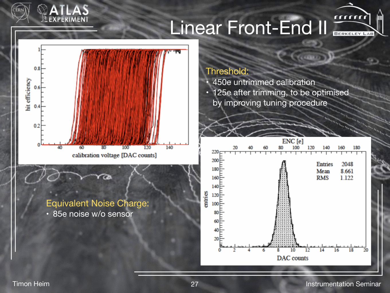
Linear Front-End II
Equivalent Noise Charge:• 85e noise w/o sensor
Threshold:• 450e untrimmed calibration• 125e after trimming, to be optimised
by improving tuning procedure
Timon Heim 28 Instrumentation Seminar
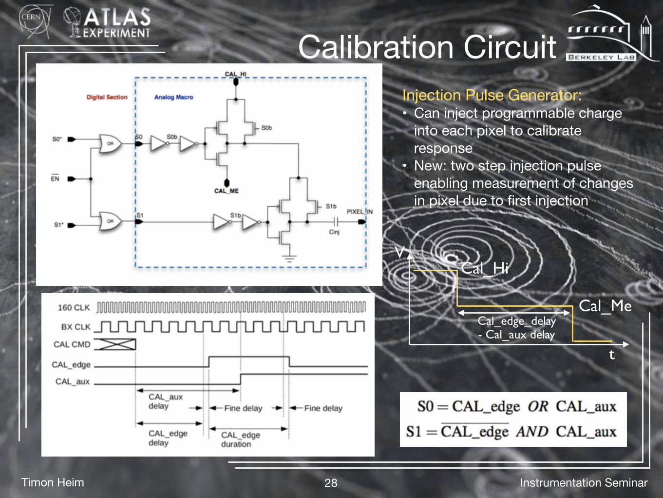
Calibration Circuit
Cal_Hi
Cal_MeCal_edge_delay- Cal_aux delay
t
V
Injection Pulse Generator:• Can inject programmable charge
into each pixel to calibrate response
• New: two step injection pulse enabling measurement of changes in pixel due to first injection
Timon Heim 29 Instrumentation Seminar
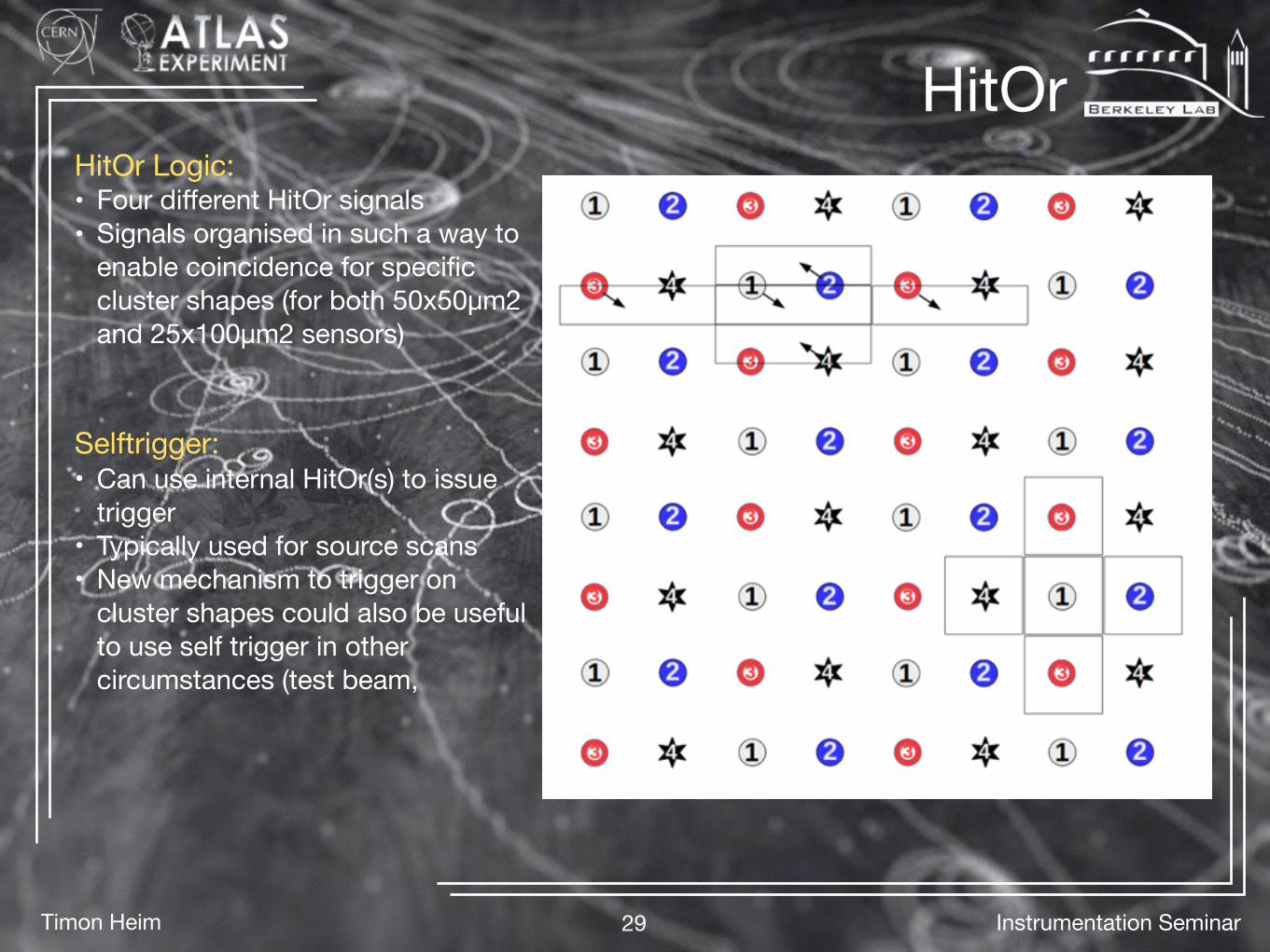
HitOrHitOr Logic:• Four different HitOr signals• Signals organised in such a way to
enable coincidence for specific cluster shapes (for both 50x50µm2 and 25x100µm2 sensors)
Selftrigger:• Can use internal HitOr(s) to issue
trigger• Typically used for source scans• New mechanism to trigger on
cluster shapes could also be useful to use self trigger in other circumstances (test beam,

Timon Heim 30 Instrumentation Seminar
I/O
\

Timon Heim 31 Instrumentation Seminar
Command InputCDR/PLL:• 160Mbps command stream• Custom encoding for DC balance• Requiring frequent sync frames to
ensure plenty of transitions
Command Encoding:• 16-bit words• Data encoded with custom 5-to-8-bit
to ensure DC balance • 15 x Trigger Cmds: 16-bit word sent
with 160Mbps covers 4 bunch crossing, need to encode all possible trigger positions
Why not 8b10b? → Synchronous trigger
Timon Heim 32 Instrumentation Seminar
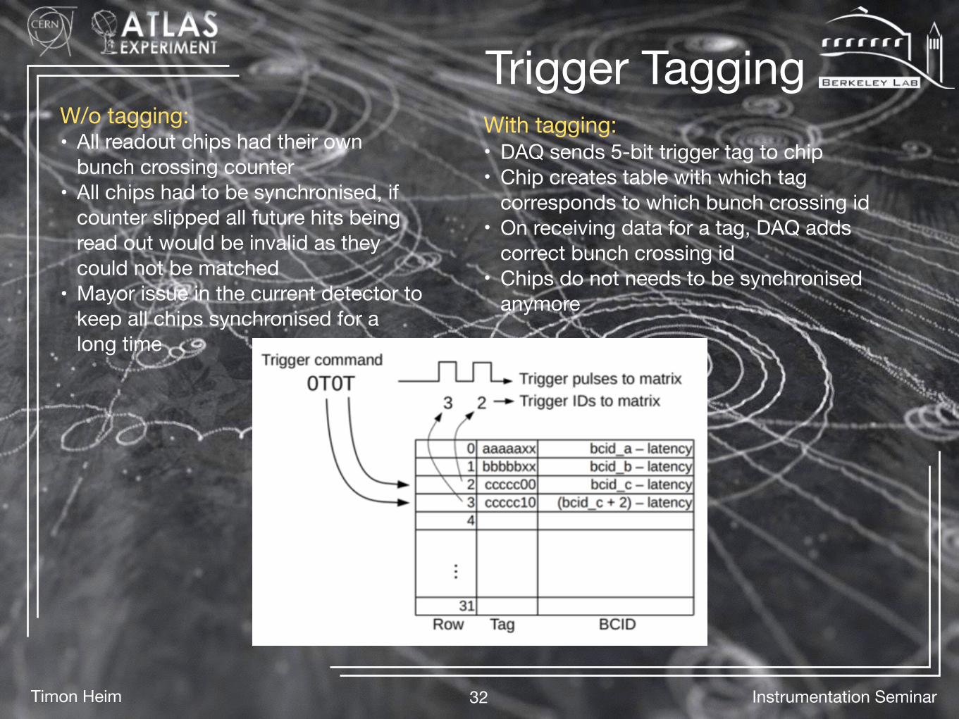
Trigger TaggingW/o tagging:• All readout chips had their own
bunch crossing counter• All chips had to be synchronised, if
counter slipped all future hits being read out would be invalid as they could not be matched
• Mayor issue in the current detector to keep all chips synchronised for a long time
With tagging:• DAQ sends 5-bit trigger tag to chip• Chip creates table with which tag
corresponds to which bunch crossing id• On receiving data for a tag, DAQ adds
correct bunch crossing id• Chips do not needs to be synchronised
anymore

Timon Heim 33 Instrumentation Seminar
Trickle ConfigurationSingle Event Upsets:• Very high SEU rate at HL-LHC• Not enough space in pixel array to
make pixel registers SEU hard• ~1% of bits corrupted by SEUs per
second• Need to avoid “de-configuration” in
some other way→ Continuously re-configure pixel (and
global registers)
WrReg[3] Sync WrReg[2] Trigger WrReg[1] WrReg[0] Trigger
Command Stream:• Need multiple 16-bit frames to write
to any register• Write/Read register commands do
not need to be contiguous, can fill gaps in between trigger/sync frames
• Cmd Stream priority:• Trigger• Sync• Write/Read Register
16-bit frame
to chip
Back of the envelope:• 1MHz trigger stream max. bandwidth is 16Mbps• 1 sync frame every 32 frames = 5Mbps• ~130Mbps available to “trickle” configuration• Full config data stream is ~350kB = 17.5ms
Timon Heim 34 Instrumentation Seminar
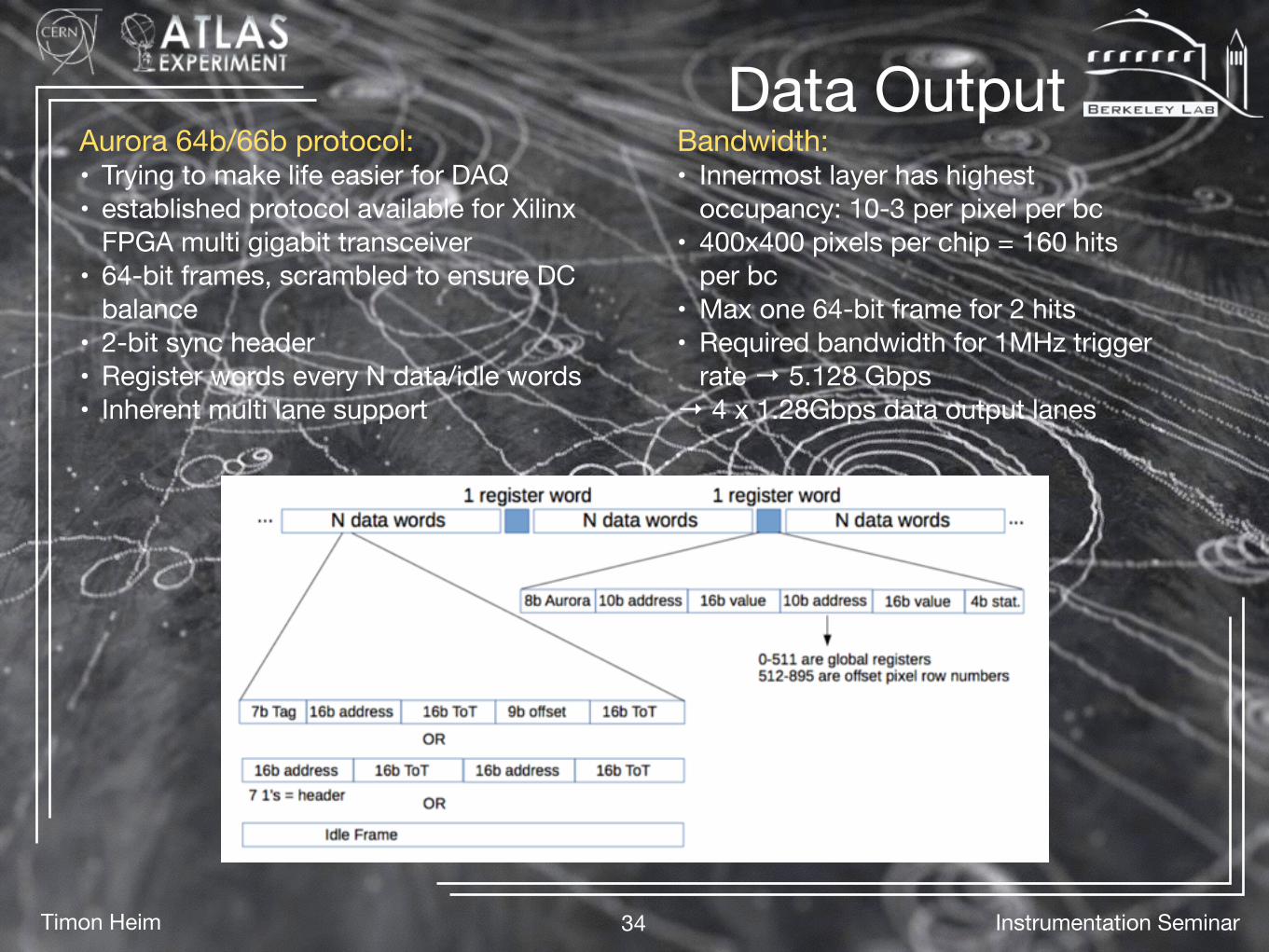
Data OutputAurora 64b/66b protocol:• Trying to make life easier for DAQ• established protocol available for Xilinx
FPGA multi gigabit transceiver• 64-bit frames, scrambled to ensure DC
balance• 2-bit sync header• Register words every N data/idle words• Inherent multi lane support
Bandwidth:• Innermost layer has highest
occupancy: 10-3 per pixel per bc• 400x400 pixels per chip = 160 hits
per bc• Max one 64-bit frame for 2 hits• Required bandwidth for 1MHz trigger
rate → 5.128 Gbps→ 4 x 1.28Gbps data output lanes

Timon Heim 35 Instrumentation Seminar
High Speed SerialiserThe Original Plan:• Need to reduce mass of detector• One 5Gbps cable has less mass than four
1.28Gbps (and less volume)• Need to transmit electrically for about ~6-9m
before we convert to optical• Cable results look promising
Reality:• Need very low jitter on 5Gbps output
(<100ps)• But we recover the clock from slow
(160Mbps) command stream• Multiplying clock and possible jitter up to
5GHz, currently too challenging• Might even result in too much jitter for
1.28Gbps (will depend on CDR/PLL performance)
Possible solutions:• Data output does not need to be
synchronous to 40MHz LHC clock• Can recover any clock in DAQ (to
some degree)• Clock serialiser from local clock
generator (e.g. lpGBT LC circuit)
5,128Gbps, 64b66b, DFE, PreEmph.

Timon Heim 36 Instrumentation Seminar
Serial Powering
ShuLDO:• Similar circuit to FE-I4 but adapted to 65nm and
~2x current• Shunt burns excess current, looks like resistor
to the outside• Can daisy chain multiple modules and run
power supply in constant current mode→ Reduces amount of necessary power cables
and therefore mass in the tracker
Example of serial powering chain:

Timon Heim 37 Instrumentation Seminar
VerificationTestbench:• UVM based verification model• Main interfaces: Hit input,
Command input, JTAG input, and Aurora output
• Automated verification components:• Pixel hit output prediction• Configuration register model
Verification types:• Constrained random test (e.g.
random hit input, or automated global register verification)
• Directed tests (custom command sequence)
• Stimuli for analog simulation

Timon Heim 38 Instrumentation Seminar
Preprations for TestingDAQ:• Using FPGA PCIe card to establish fast
link to CPU• To support 5Gbps links require Series 7
Xilinx FPGA→ Choose XpressK7 (Kintex7 FPGA)
(~1700$)• Data processing primarily done in SW
Computer
PCIe card
FE
CPU
Scan Control
Histogrammer
Scan Engine
FPGA
Aggregator
PCIe
Wafer probing:• Will perform 12-inch wafer probing• Preparations going on in IC group lab

Timon Heim 39 Instrumentation Seminar
Preparations for Testing IICooling:• In serial powering mode a single RD53A
chip will dissipate up to 4W• Quad chip modules will dissipate 16W→ Need cooling solutions which can be
used to easily support many testing setups
→ Developing Peltier based cooling setup, reducing the price per cooling unit by reusing commercial components
PC PSU Liquid CPU Cooler AIO
Arduino + MOSFET PWM controller
Peltier
Chip Mount
Module Protoyping:• RD53A flex module serial powering
chains• Test interconnect schemes• Preparations ongoing with FE-I4
Test Adapter
Quad Module
Flex cable
Timon Heim 40 Instrumentation Seminar
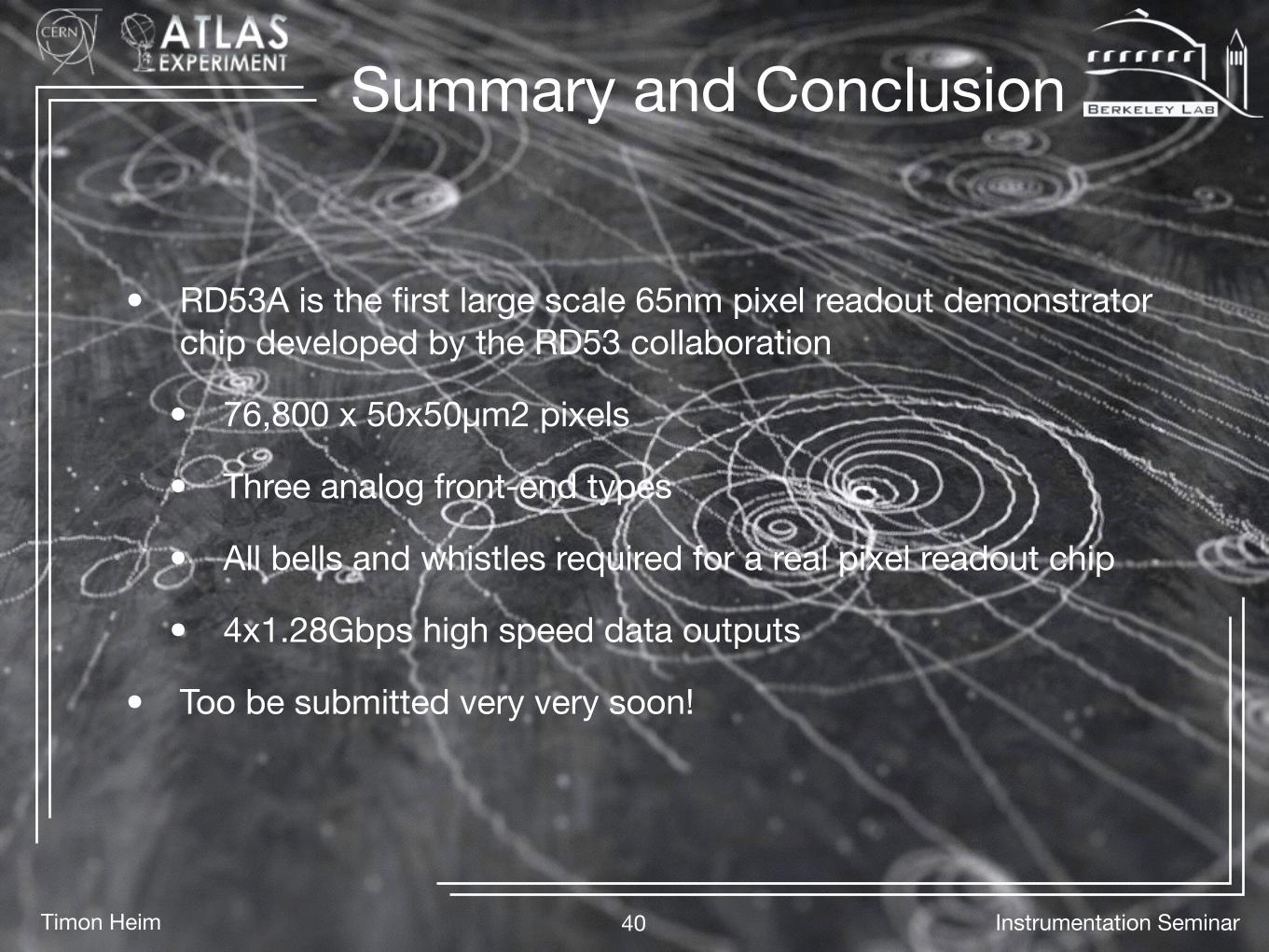
Summary and Conclusion
• RD53A is the first large scale 65nm pixel readout demonstrator chip developed by the RD53 collaboration
• 76,800 x 50x50µm2 pixels
• Three analog front-end types
• All bells and whistles required for a real pixel readout chip
• 4x1.28Gbps high speed data outputs
• Too be submitted very very soon!

Timon Heim 41 Instrumentation Seminar
Outlook for the next chip
• Many features did not make it into RD53A, but will be implemented into the ATLAS specific chip:
• 5Gbps serialiser and driver
• Non-linear ToT: increase ToT resolution in low/high ToT region
• Auto-tune mechanism: automatically tune thresholds by measuring noise occupancy
• Data compression: Use bandwidth more effectively
• 80MHz ToT counting: use both edges to count ToT
• 8-bit ToT count: combine two 4-bit memory to save one 8-bit ToT
• Event truncation: cut-off events larger than a certain size

Timon Heim 42 Instrumentation Seminar
Timon Heim 43 Instrumentation Seminar
Backup

Timon Heim 44 Instrumentation Seminar
RD53A Overview IIPowering:• Separate internal analog and digital DCDC
regulators• Integrated shunt-mode for serial powering• Estimated power consumption: 0.75A @
1.5V (1.2V internally)
Analog Front-Ends:• Contains three different types of analog
front-end for testing:• Synchronous• Linear• Differential
• All front-ends were tested in two prototype chips with 64x64 pixel:• Chipix65: Synchr. & Linear• FE65P2: Differential
Periphery:• Monitoring ADC• Reference current• Bias DACs• 2-level Injection pulse generator• Power-On-Reset• PLL
I/O:• 160Mbps custom encoded DC
balanced command input• 160MHz Clock recovery from command
stream• Trigger tagging• Four 1.28Gbps data output serialisers
using Aurora protocol• JTAG

Timon Heim 45 Instrumentation Seminar
Digital Core
Title:• Point 1• Point 2
• Point 2.1

Timon Heim 46 Instrumentation Seminar
Diff. Front-End Schematic
CSA PreComp

Timon Heim 47 Instrumentation Seminar
Sync. Front-End Schematic
CSA Krummenacher Feedback

Timon Heim 48 Meeting Name
Sync. Front-End Schematic II
Disc. Latch

Timon Heim 49 Meeting Name
Lin. Front-End Schematic
CSA Disc.

Timon Heim 50 Instrumentation Seminar
Linear Front-End III
Irradiation:• CSA working fine before and after
irradiation to 500MRad

Timon Heim 51 Instrumentation Seminar
Analog Front-End Summary
FE65P2:• 8 different flavours of analog front-ends• Picked one for RD53A which showed best
performance• Fixed some issues observed with adjusting
the feedback current
Synch. Linear Diff Spec
Charge Sensitivity [mv/ke] 43 25 103
ENC rms [e] 67 83 53 <126
Threshold Dispersion rms [e] 93 32 20 <126
In-time overdrive [e] <50 <100 0 <600
Current Consumption [µA] 3.3* 4.3 3.5 <4
ToT (6ke charge) [ns] 121 99 118 <133
*5.1µA with latch
Simulation Results for RD53A:
Chipix65:• ??