The Quantum Adiabatic Algorithm
30
The Quantum Adiabatic Algorithm Work supported by A.P. Young Talk at SMQS-IP2011, Jülich, October 18, 2011 http://physics.ucsc.edu/~peter Tuesday, October 18, 2011
Transcript of The Quantum Adiabatic Algorithm

The Quantum Adiabatic Algorithm
Work supported by
A.P. Young
Talk at SMQS-IP2011, Jülich, October 18, 2011
http://physics.ucsc.edu/~peter
Tuesday, October 18, 2011

The Quantum Adiabatic Algorithm
Work supported by
A.P. Young
Talk at SMQS-IP2011, Jülich, October 18, 2011Collaborators: V. Smelyanskiy, S. Knysh, I. Hen, E. Farhi, D. Gosset, A. Sandvik, M. Guidetti
http://physics.ucsc.edu/~peter
Tuesday, October 18, 2011

The Quantum Adiabatic Algorithm
Work supported by
A.P. Young
Talk at SMQS-IP2011, Jülich, October 18, 2011Collaborators: V. Smelyanskiy, S. Knysh, I. Hen, E. Farhi, D. Gosset, A. Sandvik, M. Guidetti
http://physics.ucsc.edu/~peter
See also poster by I. Hen and arXiv:1109.6872
Tuesday, October 18, 2011

Plan
•The Quantum Adiabatic Algorithm (QAA)
•The Quantum Monte Carlo Method (QMC)
•The Models Studied
•Results
•Comparison with a classical algorithm (WALKSAT)
•Conclusions
Here: compare the efficiency of a proposed quantum algorithm with that of a classical algorithm for solving optimization and “constraint satisfaction” problems
Question: What could we do with an eventual quantum computer in addition to Shor and Grover?
Tuesday, October 18, 2011

H(t) = [1− s(t)]HD + s(t)HP
0 ≤ s(t) ≤ 1, s(0) = 0, s(T ) = 1
�σx
i − 1�
Quantum Adiabatic AlgorithmProposed by Farhi et. al (2001) to solve hard optimization problems on a quantum computer.
0 1HD HP(g.s.) (g.s.?)adiabatic?
System starts in ground state of driver Hamiltonian. If process is adiabatic (and T → 0), it ends in g.s. of problem Hamiltonian, and problem is solved. Minimum is the “complexity”.T
T is the running time
HP is the problem Hamiltonian, depends on the σzi
HD is the driver Hamiltonian = −h�
σxi
s
Tuesday, October 18, 2011

H(t) = [1− s(t)]HD + s(t)HP
0 ≤ s(t) ≤ 1, s(0) = 0, s(T ) = 1
�σx
i − 1�
Quantum Adiabatic AlgorithmProposed by Farhi et. al (2001) to solve hard optimization problems on a quantum computer.
0 1HD HP(g.s.) (g.s.?)adiabatic?
System starts in ground state of driver Hamiltonian. If process is adiabatic (and T → 0), it ends in g.s. of problem Hamiltonian, and problem is solved. Minimum is the “complexity”.T
T is the running time
HP is the problem Hamiltonian, depends on the σzi
Is exponential or polynomial in the problem size N?T
HD is the driver Hamiltonian = −h�
σxi
s
Tuesday, October 18, 2011
Early NumericsEarly numerics, Farhi et al. for very small sizes N ≤ 20, on a particular constraint satisfaction problem found the time varied only as N2 , i.e. polynomial!
But possible “crossover” to exponential at larger sizes?
Need techniques from statistical physics, Monte Carlo.
Tuesday, October 18, 2011

0 1
HD HP
QPT
Quantum Phase Transition
Bottleneck is likely to be a quantum phase transition (QPT) where the gap to the first excited state is very small
s
Tuesday, October 18, 2011

0 1
HD HP
QPT
Quantum Phase Transition
Bottleneck is likely to be a quantum phase transition (QPT) where the gap to the first excited state is very small
s
E0
E1
minE
E
s
Tuesday, October 18, 2011

0 1
HD HP
QPT
Quantum Phase Transition
Bottleneck is likely to be a quantum phase transition (QPT) where the gap to the first excited state is very small
s
E0
E1
minE
E
s
Tuesday, October 18, 2011

0 1
HD HP
QPT
Quantum Phase Transition
Bottleneck is likely to be a quantum phase transition (QPT) where the gap to the first excited state is very small
s
E0
E1
minE
E
s
Tuesday, October 18, 2011

0 1
HD HP
QPT
Quantum Phase Transition
Bottleneck is likely to be a quantum phase transition (QPT) where the gap to the first excited state is very small
Landau Zener Theory: To stay in the ground state the time needed is proportional to ∆E−2
min
s
E0
E1
minE
E
s
Tuesday, October 18, 2011

0 1
HD HP
QPT
Quantum Phase Transition
Bottleneck is likely to be a quantum phase transition (QPT) where the gap to the first excited state is very small
Landau Zener Theory: To stay in the ground state the time needed is proportional to ∆E−2
min
s
∆EUsing QMC compute for different s: → ΔEmin
E0
E1
minE
E
s
Tuesday, October 18, 2011

Quantum Monte CarloWe do a sampling of the 2N states (so statistical errors).
Study equilibrium properties of a quantum system by simulating a classical model with an extra dimension, imaginary time, τ, where 0 ≤ τ < 1/T.
Not perfect, but the only numerical method available for large N.
We use the “stochastic series expansion” method for Quantum Monte Carlo simulations which was pioneered by Anders Sandvik.
Z ≡ Tre−βH =∞�
n=0
Tr (−βH)n
n!
Stochastically sum the terms in the series.
Tuesday, October 18, 2011

�A(τ )A(0)� − �A�2 =�
n�=0
|�0|A|n�|2 exp[−(En − E0)τ ]
0.001
0.01
0.1
1
0 10 20 30 40 50
C(
)
3-reg MAX-2-XORSAT, N = 128
QMC fit, E = 0.090
0.001
0.01
0.1
1
10
0 5 10 15 20 25 30
<Hp(
)Hp(
0)>
- <H
p>2
3-reg MAX-2-XORSAT, N=24
= 64, symmetric levels
diag.QMC
Examples of results with the SSE codeTime dependent correlation functions decay with τ as a sum of exponentials
For large τ only first excited state contributes, → pure exponential decay
Small size, N= 24, excellent agreement with diagonalization.
Large size, N = 128, good quality data, slope of straight line → gap.
Tuesday, October 18, 2011
Satisfiability Problems I In satisfiability problems (SAT) we ask whether there is an assignment of N bits which satisfies all of M logical conditions (“clauses”). We assign an energy to each clause such that it is zero if the clause is satisfied and a positive value if not satisfied.
i.e. We need to determine if the ground state energy is 0.
We take the ratio of M/N to be at the satisfiability threshold, and study instances with a “unique satisfying assignment” (USA). (so gap to 1st excited state has a minimum whose value indicates the complexity.)
Tuesday, October 18, 2011
Satisfiability Problems II • Locked 1-in-3 SATThe clause is formed from 3 bits picked at random. The clause is satisfied (has energy 0) if 1 is one and the other two are zero. Otherwise it is not satisfied (and the energy is 1).• Locked 2-in-4 SATSimilar to 1-in-3 but the clause has 4 bits and is satisfied if 2 of them are one. (This has bit-flip symmetry).
“Locked” means that each bit is in at least two clauses, and flipping one bit in a satisfying assignment makes it unsatisfied.
Satisfiability threshold at critical value of M/N. We work at this threshold, (hard, Kirkpatrick and Selman) and take instances with a “USA”. These seem to be a finite fraction of whole ensemble even for N ➝ ∞.
Tuesday, October 18, 2011

Satisfiability Problems III • 3-spin model (3-regular 3-XORSAT)
3-regular means that each bit is in exactly three clauses. 3-XORSAT means that the clause is satisfied if the sum of the bits (mod 2) is a value specified (0 or 1) for each clause.In terms of spins σz (= ±1) we require that the product of the three σz’s in a clause is specified (+1 or -1).
(Is at SAT threshold.)This SAT problem can be solved by linear algebra (Gaussian elimination) and so is in P. Nonetheless we will see that it is very hard for heuristic algorithms (quantum and classical).
HP =M�
α=1
12
�1 − Jα σz
α,1σzα,2σz
α,3
�
Tuesday, October 18, 2011

0.01
0.1
10 100m
edia
n E m
in
N
2 / ndf = 18.73Q = 3.82e-12
5.6 N-1.51
0.001
0.01
0.1
10 20 30 40 50 60 70 80 90 100
med
ian
E min
N
2 / ndf = 1.35Q = 0.26
0.16 exp(-0.042 N)
Locked 1-in-3
Clearly the behavior of the minimum gap is exponential
Exponential fit Power law fit
Plots of the median minimum gap
Tuesday, October 18, 2011
0.01
0.1
10 20 30 40 50
med
ian
E min
N
2 / ndf = 4.27Q = 0.005
7.6 N-1.50
0.01
0.1
10 20 30 40 50 60
med
ian
E min
N
2 / ndf = 1.31Q = 0.27
0.32 exp(-0.063 N)
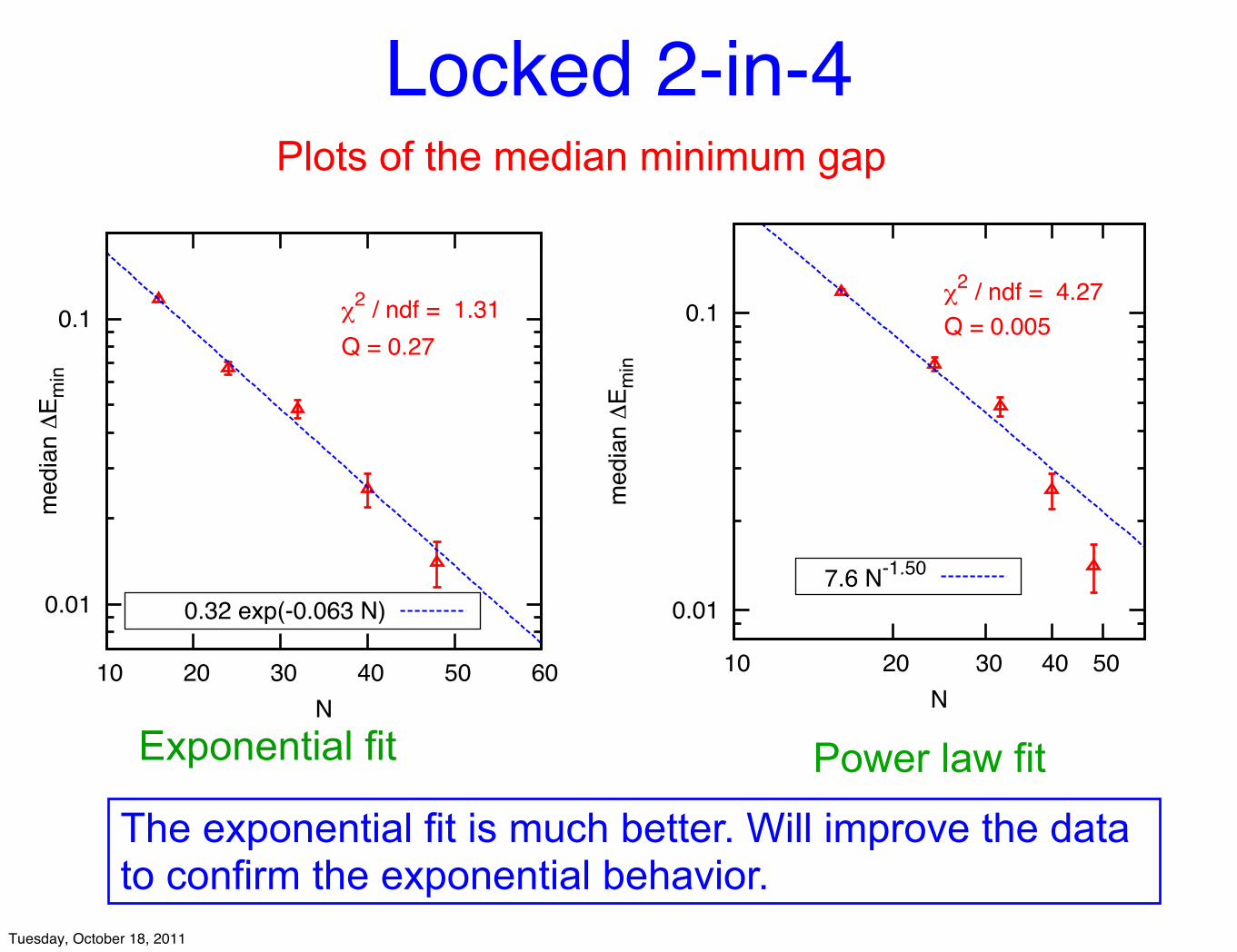
Locked 2-in-4Plots of the median minimum gap
Exponential fit Power law fit
The exponential fit is much better. Will improve the data to confirm the exponential behavior.
Tuesday, October 18, 2011

0
1
2
3
4
5
6
7
0 0.2 0.4 0.6 0.8 1
E n
s
3-reg XORSAT (1 instance, N = 16)
E3E2E1E0
3-Reg 3-XORSAT (3-spin model): I
Curves for energies on left are very close to symmetric about s = 1/2. There is an exact duality where the dual lattice interchanges the clauses and bits (i.e. is a different member of the ensemble), see the “factor graph” above right. Hence the phase transition is exactly at the self dual point s=1/2.
Tuesday, October 18, 2011

0.01
0.02
0.04
0.06 0.08
0.1
10 15 20 25 30 35 40
med
ian
E min
N
3-reg XORSAT
diagQMC
0.22 exp(-0.080 N)
3-Reg 3-XORSAT: IIExponential (i.e. log-lin) plot of the median minimum gap
Clearly the minimum gap is exponential, even for small NTuesday, October 18, 2011

Comparison with a classical algorithm, WalkSAT: I
WalkSAT is a classical, heuristic, local search algorithm. It is a reasonable classical algorithm to compare with QAA.We have compared the running time of the QAA for the three SAT problems studied with that of WalkSAT.For QAA, Landau-Zener theory states that the time is proportional to 1/(ΔEmin)2 (neglecting N dependence of matrix elements).For WalkSAT the running time is proportional to number of “bit flips”.We write the running time as proportional to We will compare the values of µ among the different models and between QAA and WalkSAT.
exp(µ N).
Tuesday, October 18, 2011

101
102
103
104
105
106
107
108
109
0 50 100 150 200 250 300m
edia
n fli
psN
WalkSAT
3-XORSAT, 158 exp(0.120 N)2-in-4, 96 exp(0.086 N)
1-in-3, 496 exp(0.050 N) 0.001
0.01
0.1
10 20 30 40 50 60 70 80 90 100
med
ian
E min
N
QAA
1-in-3, 0.16 exp(-0.042 N)2-in-4, 0.32 exp(-0.063 N)
3-XORSAT, 0.22 exp(-0.080 N)
Comparison with a classical algorithm, WalkSAT: II
The trend is the same in both QAA and WalkSAT. 3-XORSAT is the hardest, and locked 1-in-3 SAT the easiest.
Exponential behavior for both QAA and WalkSAT
Tuesday, October 18, 2011

Comparison with a classical algorithm, WalkSAT: III
Values of µ (where time ~ exp[µ N]).
Model QAA WalkSAT Ratio
1-in-3 0.084(3) 0.0505(5) 1.66
2-in-4 0.126(7) 0.0858(8) 1.47
3-XORSAT 0.159(2) 0.1198(4) 1.32
These results used the simplest implementation of the QAA for instances with a USA. Interesting to also study random instances to see if they also have exponential complexity in QAA. Also look for better paths in Hamiltonian space.
Tuesday, October 18, 2011

i3
1 2
3-Reg MAX-2-XORSAT: IWe have also studied one “MAX” (i.e. optimization) problem.
MAX means we are in the UNSAT phase, and want to find the configuration with the least number of unsatisfied clauses.
We take the “antiferromagnet” version, i.e. the energy is zero if the bits are different (otherwise it is 1). 3-Regular means that it bit is in three clauses, i.e. has 3 “neighbors” connected to it. The connected pairs are chosen at random.
Note: there are large loops
The “2” in 2-XORSAT means each clause has 2 bits. “Replica” theory indicates that 2-SAT-like problems are different from K-SAT problems for K > 2.
Tuesday, October 18, 2011
HP =12
�
�i,j�
�1 + σz
i σzj
�
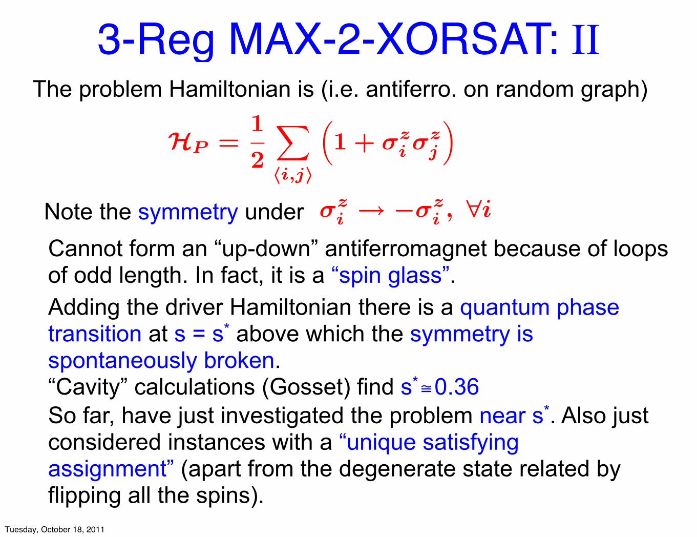
3-Reg MAX-2-XORSAT: IIThe problem Hamiltonian is (i.e. antiferro. on random graph)
σzi → −σz
i , ∀iNote the symmetry under Cannot form an “up-down” antiferromagnet because of loops of odd length. In fact, it is a “spin glass”.Adding the driver Hamiltonian there is a quantum phase transition at s = s* above which the symmetry is spontaneously broken.“Cavity” calculations (Gosset) find s*≅0.36So far, have just investigated the problem near s*. Also just considered instances with a “unique satisfying assignment” (apart from the degenerate state related by flipping all the spins).
Tuesday, October 18, 2011

0.1
0.2
0.3
20 40 60 80 100 120 140
E min
N
3-reg MAX-2-XORSAT
2 / ndf = 1.10Q = 0.29
0.29 exp(-0.014 N)
0.05
0.1
0.2
0.3
10 100
E min
N
3-reg MAX-2-XORSAT
power-law fit2 / ndf = 1.90
Q = 0.13
3.16 N-0.823
3-Reg MAX-2-XORSAT: III
Power-law fit Exponential fit omitting 1st 2 points
Median minimum gap in the vicinity of the quantum transition
Looks like power law, but exponential (plus corrections at small sizes) can’t be excluded. Larger sizes will be done to check.
Tuesday, October 18, 2011

Conclusions• Simple application of QAA gives exponentially small gaps
for SAT problems with a USA.(same conclusion as in the talk by Thomas Neuhaus).• An optimization problem, MAX-2-SAT, looks more
promising, but needs data at larger sizes to be sure.• Need to see if the exponentially small gap can be removed
by• repeatedly running the algorithm with different random
values for the transverse fields (and costs). • trying to find a clever way to optimize the path in
Hamiltonian space “on the fly” during the simulation to increase the minimum gap.• considering random instances rather than instances with
a USA.
Tuesday, October 18, 2011

![arXiv:1909.05500v2 [quant-ph] 9 Jan 2020 · 2020-01-10 · Quantum linear system solver based on time-optimal adiabatic quantum computing and quantum approximate optimization algorithm](https://static.fdocuments.us/doc/165x107/5f3a70883c192e455e649391/arxiv190905500v2-quant-ph-9-jan-2020-2020-01-10-quantum-linear-system-solver.jpg)