
Adiabatic quantum computing from an eigenvalue dynamics ... · Loughborough University...
110
•
Transcript of Adiabatic quantum computing from an eigenvalue dynamics ... · Loughborough University...

Loughborough UniversityInstitutional Repository
Adiabatic quantumcomputing from an
eigenvalue dynamics point ofview
This item was submitted to Loughborough University's Institutional Repositoryby the/an author.
Additional Information:
• A Doctoral Thesis. Submitted in partial ful�llment of the requirementsfor the award of Doctor of Philosophy of Loughborough University.
Metadata Record: https://dspace.lboro.ac.uk/2134/8780
Publisher: c© Richard D. Wilson
Please cite the published version.

This item was submitted to Loughborough’s Institutional Repository (https://dspace.lboro.ac.uk/) by the author and is made available under the
following Creative Commons Licence conditions.
For the full text of this licence, please go to: http://creativecommons.org/licenses/by-nc-nd/2.5/

Adiabatic quantum computing from an eigenvalue
dynamics point of view
by Richard D. Wilson
A Doctoral Thesis submitted in partial fulfillment of the requirements
for the award of
Doctor of Philosophy
of
Loughborough University
July 2011
c©Richard D. Wilson 2011

Abstract
We investigate the effects of a generic noise source on a prototypical adiabatic quan-
tum algorithm. We take an alternative eigenvalue dynamics viewpoint and derive
a generalised, stochastic form of the Pechukas-Yukawa model. The distribution of
avoided crossings in the energy spectra is then analysed in order to estimate the
probability of level occupation.
We find that the probability of successfully finding the system in the solution
state decreases polynomially with the computation speed and that this relationship
is independent of the noise amplitude. The overall regularity of the eigenvalue dy-
namics is shown to be relatively unaffected by noise perturbations. These results
imply that adiabatic quantum computation is a relatively stable process and pos-
sesses a degree of resistance against the effects of noise. We also show that generic
noise will inherently break any symmetries, and therefore remove degeneracies, in
the energy spectrum that might otherwise have impeded the computation process.
This suggests that the conventional stipulation that the initial and final Hamilto-
nians do not commute is unnecessary in realistic physical systems. We explore the
effects of an artificial noise source with a specifically engineered time-dependent am-
plitude and show that such a scheme could provide a significant enhancement to the
performance of the computation.
Finally, we formulate an extended version of the Pechukas-Yukawa formalism.
This provides a complete description of the dynamics of a quantum system by way
of an exact mapping to a system of classical equations of motion.

Contents
1 Introduction 1
1.1 Thesis overview . . . . . . . . . . . . . . . . . . . . . . . . . . . . . . 3
1.2 Quantum information processing devices . . . . . . . . . . . . . . . . 3
1.2.1 Basic postulates and notation . . . . . . . . . . . . . . . . . . 3
1.2.2 Quantum computing . . . . . . . . . . . . . . . . . . . . . . . 5
1.2.3 Adiabatic quantum computing . . . . . . . . . . . . . . . . . . 7
1.2.3.1 Basic principles . . . . . . . . . . . . . . . . . . . . . 7
1.2.3.2 Algorithms . . . . . . . . . . . . . . . . . . . . . . . 10
1.2.3.3 The GSQC method . . . . . . . . . . . . . . . . . . . 12
1.2.3.4 Noise and decoherence . . . . . . . . . . . . . . . . . 13
1.2.3.5 Physical realisations . . . . . . . . . . . . . . . . . . 15
1.3 Eigenvalue dynamics . . . . . . . . . . . . . . . . . . . . . . . . . . . 17
1.4 Random matrices . . . . . . . . . . . . . . . . . . . . . . . . . . . . . 18
2 Generalised Pechukas-Yukawa model 21
2.1 Generalised Pechukas-Yukawa equations . . . . . . . . . . . . . . . . 21
2.2 Random matrix Noise model . . . . . . . . . . . . . . . . . . . . . . . 26
2.3 Numerical methods and testing . . . . . . . . . . . . . . . . . . . . . 27
3 The CNOT gate 32
3.1 The CNOT problem Hamiltonian . . . . . . . . . . . . . . . . . . . . 32
3.2 Initial conditions . . . . . . . . . . . . . . . . . . . . . . . . . . . . . 34
4 The energy spectra of the CNOT gate 36
5 The statistics of level occupation for the CNOT gate 48
6 The CNOT gate with an artificial noise source 58
7 The extended Pechukas-Yukawa system 62
i

CONTENTS ii
8 Conclusions 66
8.1 Suggestions for further work . . . . . . . . . . . . . . . . . . . . . . . 67
A Program listings 71
A.1 Simulation programs . . . . . . . . . . . . . . . . . . . . . . . . . . . 71
A.2 Analysis programs . . . . . . . . . . . . . . . . . . . . . . . . . . . . 76
B Noise-enhanced performance of adiabatic quantum computing by
lifting degeneracies 80
C The relationship between minimum gap and success probability in
adiabatic quantum computing 87

List of Figures
1.2.1 Schematic diagram of a generic adiabatic quantum computation where
the system is prepared in the ground state of the initial Hamiltonian
(Hi) and then evolves adiabatically slowly to a final Hamiltonian (Hf )
that encodes the problem. . . . . . . . . . . . . . . . . . . . . . . . . 8
1.2.2 Schematics of a single flux qubit and a device consisting of three
coupled flux qubits . . . . . . . . . . . . . . . . . . . . . . . . . . . . 16
2.3.1 Example showing a critical point in the energy spectrum of an adi-
abatic quantum computer, namely an avoided crossing between the
ground and first excited state. . . . . . . . . . . . . . . . . . . . . . . 29
2.3.2 Plots showing a comparison of the energy spectrum calculated using
the generalised Pechukas-Yukawa model and the results of direct di-
agonalisation (crosses) for a 4-qubit system with GUE Hamiltonians
and GOE random matrix noise where Z = 10, ε = 0.1 and τ = 0.1. . . 30
2.3.3 Flowchart describing algorithm used to estimate the occupation prob-
abilities as a function of time for a given energy spectrum. . . . . . . 31
3.1.1 Schematic of the quantum dot array used to encode a CNOT gate
into Hamiltonian form using the GSQC method. . . . . . . . . . . . . 33
4.0.1 The energy spectra of the 4 operations of the adiabatic CNOT gate
in the absence of noise. . . . . . . . . . . . . . . . . . . . . . . . . . . 38
4.0.2 Plot showing the particle velocities (vn(λ)) for the |00〉 → |00〉 oper-
ation of the CNOT gate in the absence of noise. . . . . . . . . . . . . 39
4.0.3 Plot showing the non-zero particle-particle coupling strengths (lmn(λ))
for the |00〉 → |00〉 operation of the CNOT gate in the absence of noise. 39
4.0.4 The energy spectra of the 4 possible operations of the adiabatic
CNOT gate in the presence of coloured noise of amplitude ε = 0.1. . . 41
4.0.5 Plot showing the particle velocities (vn(λ)) for the |00〉 → |00〉 oper-
ation of the CNOT gate in the presence of coloured noise. . . . . . . 42
iii
LIST OF FIGURES iv
4.0.6 Plot showing the particle-particle coupling strengths (lmn(λ)) for the
|00〉 → |00〉 operation of the CNOT gate in the presence of coloured
noise. . . . . . . . . . . . . . . . . . . . . . . . . . . . . . . . . . . . . 42
4.0.7 The distribution of average gap widths (∆m,m+1) at avoided crossings
in the energy spectrum of the CNOT gate |00〉 → |00〉 operation at a
range of noise amplitudes. . . . . . . . . . . . . . . . . . . . . . . . . 43
4.0.8 Distribution of minimum ground state energy gaps for the |00〉 → |00〉and |01〉 → |01〉 operations. . . . . . . . . . . . . . . . . . . . . . . . 44
4.0.9 Distribution of energy gap widths for state in the bulk of the spectrum
for the |01〉 → |01〉 operation. . . . . . . . . . . . . . . . . . . . . . . 45
4.0.10The Brody parameter, q, as a function of ‘time’ for all four opera-
tions of the CNOT gate with ε = 0 and 0.1. These values of q are
found by fitting the Brody distribution to the unfolded nearest neigh-
bour spacing distribution and the average value of the coefficient of
determination was R2 = 0.7488. . . . . . . . . . . . . . . . . . . . . . 47
5.0.1 Plot of average success probability against computation speed for the
|00〉 → |00〉 operation of the CNOT gate at various noise amplitudes. 50
5.0.2 Plot of average occupation of the lowest 5 levels at λ(t) = 0 for the
|00〉 → |00〉 operation at ε = 0.025 and 0.1. . . . . . . . . . . . . . . . 51
5.0.3 Plot of average success probability against computation speed for the
|01〉 → |01〉 operation of the CNOT gate at various noise amplitudes. 52
5.0.4 Plot of average occupation of the lowest 5 levels at λ(t) = 0 for the
|01〉 → |01〉 operation at ε = 0.1. . . . . . . . . . . . . . . . . . . . . . 53
5.0.5 Plot of average success probability against computation speed for the
|10〉 → |11〉 operation of the CNOT gate at various noise amplitudes. 53
5.0.6 Plot of average success probability against computation speed for the
|11〉 → |10〉 operation of the CNOT gate at various noise amplitudes. 54
5.0.7 Plot showing the average fidelity of the final state and average success
probability as functions of noise amplitude for the |00〉 → |00〉 operation. 55
5.0.8 Plot showing the average fidelity of the final state and average success
probability as functions of noise amplitude for the |01〉 → |01〉 operation. 56
5.0.9 Plot showing the average fidelity of the final state and average success
probability as functions of noise amplitude for the |10〉 → |11〉 operation. 56
5.0.10Plot showing the average fidelity of the final state and average success
probability as functions of noise amplitude for the |11〉 → |10〉 operation. 57

LIST OF FIGURES v
6.0.1 Plot of average success probability against computation speed for the
|00〉 → |00〉 operation of the CNOT gate with an artificial noise source
at a range of values for ε0 and α = 10. For comparative purposes, the
results for a noise source with a constant amplitude of ε = 0.025 are
also shown. . . . . . . . . . . . . . . . . . . . . . . . . . . . . . . . . 60
6.0.2 Plot of average success probability against computation speed for the
|01〉 → |01〉 operation of the CNOT gate with an artificial noise source
at a range of values for ε0 and α = 10. For comparative purposes,
the results for a noise source with a constant amplitude of ε = 0.1 are
also shown. . . . . . . . . . . . . . . . . . . . . . . . . . . . . . . . . 60
6.0.3 Plot of average success probability against computation speed for the
|10〉 → |11〉 operation of the CNOT gate with an artificial noise source
at a range of values for ε0 and α = 10. For comparative purposes,
the results for a noise source with a constant amplitude of ε = 0.1 are
also shown. . . . . . . . . . . . . . . . . . . . . . . . . . . . . . . . . 61
6.0.4 Plot of average success probability against computation speed for the
|11〉 → |10〉 operation of the CNOT gate with an artificial noise source
at a range of values for ε0 and α = 10. For comparative purposes,
the results for a noise source with a constant amplitude of ε = 0.1 are
also shown. . . . . . . . . . . . . . . . . . . . . . . . . . . . . . . . . 61

Acknowledgements
I would like to sincerely thank my supervisors; Dr Alexandre Zagoskin and Dr
Sergey Savel’ev, for their support and guidance over the course of my PhD, it has
been invaluable. I would also like to thank my friends and family for their con-
tinual support and encouragement along the way. Finally, I would like to thank
Loughborough University for my studentship and support for various conferences.
vi

Chapter 1
Introduction
“And therefore, the problem is, how can we simulate the quantum
mechanics? There are two ways that we can go about it. We can give
up on our rule about what the computer was, we can say: Let the
computer itself be built of quantum mechanical elements which obey
quantum mechanical laws. Or we can turn the other way and say: Let
the computer still be the same kind that we thought of before–a logical,
universal automaton; can we imitate this situation?” - R.P. Feynman [1]
Interest and research in the field of quantum engineering has steadily grown over
recent years. This is because it offers a direct opportunity to experiment with and
even utilise the very phenomena that differentiate the quantum mechanical picture
of the universe from that of the classical one.
Quantum computing is one area of quantum engineering in particular that has
received a lot of attention since the discoveries of Shor’s factoring algorithm [2], and
Grover’s search algorithm [3] during the 1990’s. Both of these algorithms demon-
strate the power of harnessing explicitly quantum mechanical processes to perform a
computational process. This allows them to perform in a more efficient manner than
is possible using classical resources. The idea of storing and processing information
quantum mechanically was first proposed by Feynman in 1981, [1], while discussing
the problems of simulating physics with computers. Simulating quantum mechanical
systems on a classical computer is a computationally demanding task as the number
of dimensions of the phase space needed to describe the state of the quantum system
scales exponentially with its size. Hence, Feynman proposed the idea of building
a computer that works and stores information on a quantum mechanical level so
it can inherently work with the high dimensional phase spaces needed to describe
these quantum systems. The concept of a quantum computer was later solidified by
Deutsch in 1985 [4] when he defined a quantum generalisation of the classical uni-
1

CHAPTER 1. INTRODUCTION 2
versal Turing machine. Deutsch, in conjunction with Jozsa, then went on to develop
one of the first quantum algorithms that could be shown to be exponentially faster
than any possible classical deterministic counterpart [5]. Although the Deutsch-
Jozsa algorithm is of little practical use, it paved the way for further research in to
whether quantum mechanical information processing techniques could be used to
solve other computational problems. The discovery of Shor’s aforementioned fac-
toring algorithm [2], which offers an exponential speedup in time over its classical
counterparts, and Grover’s search [3], which offers a polynomial speedup, showed
that quantum computing could offer significant improvements in computational ef-
ficiency for practical real world problems. Since then a number of other quantum
algorithms have been discovered for a wide variety of different problems (an up to
date list of which can be found at http://www.its.caltech.edu/ sjordan/zoo.html).
The standard paradigm of quantum computing that has developed over recent
years is analogous to a classical digital computer, as a register of qubits (quantum
bits) are manipulated using a universal set of quantum logic gates. However, this ap-
proach requires a delicate balance between attempting to isolate the system from its
environment but at the same time maintaining precise control over individual qubits,
which unfortunately appears as though it may not be experimentally achievable in
the near future. In light of this realisation a number of alternative approaches have
been proposed; one of which is adiabatic quantum computing (AQC) [6]. AQC in-
volves slow adiabatic evolution from a configuration with an easily reachable ground
state to one where the ground state encodes the solution to the problem in hand. In
this scheme precise time-dependent control of individual qubits is no longer required
and it benefits from an inherent robustness against some of the effects of decoher-
ence by remaining in the instantaneous ground state at all times [7, 8, 9]. Crucially,
it has also been shown to be polynomially equivalent to the standard gate model
of quantum computing in [10, 11]. There have also been some results that suggest
that noise may actually have some positive effects on an AQC process, which is an
interesting and counter-intuitive prospect [7, 12].
In this thesis we aim to further explore the role and effects of noise in the
paradigm of adiabatic quantum computing. This is clearly an important consid-
eration as all realistic physical systems will be subject to some form of noise. To do
this we will make use of a novel eigenvalue dynamics based approach. It is felt that
this approach is worth exploring as it offers an alternative viewpoint to the standard
Schrodinger picture which may provide some extra insight.

CHAPTER 1. INTRODUCTION 3
1.1 Thesis overview
The remainder of this chapter will be devoted to a review of the field of AQC and
some theoretical tools that will be of use in the following chapters. In chapter 2,
we derive a generalised form of the Pechukas-Yukawa model of eigenvalue dynamics
that incorporates a generic noise model. Appropriate numerical methods for solving
this system of equations are also discussed.
In chapter 3, we derive the problem Hamiltonian for the adiabatic equivalent of
the CNOT gate as an example of a prototypical quantum algorithm. Then in the
following chapters 4, 5 and 6, we go on to explore how the presence of noise affects
the properties and performance of this example algorithm. In chapter 4, we study
the energy spectra of the CNOT gate and look at the effects of noise on its statistical
properties. We investigate the effects of noise on the statistics of level occupation
and the success rate of the CNOT algorithm in chapter 5. Based on the previous
results, in chapter 6 we envision a system where a specifically engineered noise signal
is used to enhance the performance of our prototypical quantum algorithm.
Also, in chapter 7, we derive a novel extended version of the Pechukas-Yukawa
model that provides a complete description of the dynamics of the quantum system.
Then in chapter 8 we draw together our results and make some final conclusions,
as well as proposing a number of possible directions in which this work could be
taken in the future.
1.2 Quantum information processing devices
1.2.1 Basic postulates and notation
In this section we will briefly review the basic postulates of quantum mechanics,
mainly as a way of codifying the notation used throughout this thesis. The four
basic postulates of quantum mechanics that can be used to describe any closed
system are as follows;
1. State: The state of any closed quantum system at a particular point in time
is completely described by the state vector, |ψ(t)〉, which is a unit vector in
the Hilbert space associated with the system’s degrees of freedom.
2. Evolution: The evolution of a closed quantum system is described by a uni-
tary transformation, i.e. the state |ψ (t1)〉 is related to the state |ψ′ (t2)〉 by
|ψ′ (t2)〉 = U (t1, t2) |ψ (t1)〉, where U (t1, t2) is a unitary operator (i.e. one
that obeys UU † = U †U = I) that depends only on the times t1 and t2. In

CHAPTER 1. INTRODUCTION 4
terms of continuous time, the unitary evolution of a closed quantum system is
generated by the Schrodinger equation
i~d
dt|ψ(t)〉 = H(t) |ψ(t)〉 , (1.2.1)
where ~ is Planck’s constant (taken as 1 from herein) andH(t) is the Hermitian
operator (i.e. one that obeys H = H†)known as the Hamiltonian.
3. Measurement: Quantum measurements are described by a set of measure-
ment operators, {Mm}, that act on the state space of the system and satisfy
the completeness relation∑
m M†m Mm = 1. If a measurement is performed on
a system in state |ψ(t)〉, then the probability of result m occurring is given by
p(m) = 〈ψ(t)|M†m Mm |ψ(t)〉 (1.2.2)
and after the measurement the state of the system “collapses” to
Mm |ψ(t)〉√〈ψ(t)|M†m Mm |ψ(t)〉
. (1.2.3)
4. Composite systems: Composite systems, made up of a number (n) of dis-
tinct physical systems, have a state space that is the tensor product of the
state spaces of the constituent subsystems. A composite system is said to
be in a product or separable state if its state be constructed from the tensor
product of the subsystem’s states, i.e.|ψ1(t)〉 ⊗ |ψ2(t)〉 . . . |ψn(t)〉. Whereas an
entangled state is defined as one where the overall state of composite system
cannot be described in terms of single qubit states.
The Hamiltonian operator, H(t), of a system is crucial, as if we have knowledge
of this, then we can completely describe the dynamics of the system. In terms of this
thesis, an important point to note is that because the Hamiltonian is a Hermitian
operator it will have an instantaneous spectral decomposition of the form
H(t) =∑n
xn(t) |n(t)〉 〈n(t)| , (1.2.4)
where the xn(t) are the instantaneous eigenvalues describing the energy levels of the
system at time t, and the |n(t)〉 are their corresponding normalised eigenvectors,
known as the eigenstates. The collection of all n eigenstates forms the instantaneous
energy eigenbasis of the Hamiltonian at time t. These energy levels and eigenstates

CHAPTER 1. INTRODUCTION 5
satisfy the following instantaneous eigenvalue equation;
H(t) |n(t)〉 = xn(t) |n(t)〉 , (1.2.5)
which is simply the time-independent version of the Schrodinger equation.
In some situations it is often more convenient to work with the density matrix,
or density operator, instead of the state vector. This is defined as
ρ =∑i
pi |i〉 〈i| , (1.2.6)
where pi is the probability of the system being found in a given pure state |i〉. This
alternative formulation is particularly suited to dealing with statistical mixtures of
states and is often used when dealing with dissipation and composite systems. The
equation of motion for the density matrix is the Von Neumann equation,
i~d
dtρ(t) = [H(t), ρ(t)] . (1.2.7)
The density matrix formulation will be of particular use in chapter 7.
1.2.2 Quantum computing
In [4], Deutsch showed that the Church-Turing principle,
“Every finitely realisable physical system can be perfectly simulated by
a universal model computing machine operating by finite means”.
(restated in a more physical way), is compatible with quantum mechanics and that
any real (dissipative) finite system can be simulated by a universal quantum com-
puter. As mentioned in section 1, he then went on to describe the first universal
model of quantum computation, essentially a quantum generalisation of a Turing
machine [13]. Unfortunately, like the Turing machine before it, this model of uni-
versal quantum computation proved unwieldy in practical situations. An equivalent
model more akin to classical digital computation, where logic gates are applied to
a register of quantum bits (qubits), was then developed. This is commonly known
as the quantum circuit or gate model. In [14], DiVincenzo proposed a set of five
requirements for a physical implementation of a gate model quantum computer.
These criteria allow us to completely describe the operation of a gate model quan-
tum computer;
1. A scalable physical system with well characterized qubits

CHAPTER 1. INTRODUCTION 6
2. The ability to initialize the state of the qubits to a simple fiducial state, such
as |0000...0〉
3. Long relevant decoherence times, much longer than the gate operation time
4. A “universal” set of quantum gates
5. A qubit-specific measurement capability
The first DiVincenzo criterion calls for scalable, well characterised qubits. As a
qubit is the quantum analogue of a bit, it is simply a two-level quantum system.
The 0 and 1 states of a classical bit correspond to the computational basis states of
a qubit,
|0〉 =
(1
0
)and |1〉 =
(0
1
), (1.2.8)
therefore a qubit in an arbitrary state can be described by
|ψ〉 = α |0〉+ β |1〉 =
(α
β
)where 〈ψ|ψ〉 = |α|2 + |β|2 = 1. (1.2.9)
In the density matrix formulation, the state of a qubit can be expressed as follows;
ρ =I + r · σ
2, (1.2.10)
where r = (x, y, z) is the Bloch vector which describes a point in the Bloch sphere
and σ = (σx, σy, σz) is a vector of the Pauli matrices;
σx =
(0 1
1 0
), σy =
(0 −ii 0
), σz =
(1 0
0 −1
). (1.2.11)
The Bloch sphere is a unit sphere which provides a convenient geometrical repre-
sentation of a qubit’s state space. The Bloch vector of pure states will lie on the
surface of the sphere, whereas the points representing mixed states will fall within
it. There are a number of different candidates for physical realisations of qubits,
e.g. single electrons, trapped ions, superconducting circuits and laser polarisation,
these will be discussed in more detail in section 1.2.3.5.
The fourth criterion asks for a “universal” set of quantum gates, this is a set
of gates with which any arbitrary quantum operation can be reproduced. A simple
example of which would be the set of the Hadamard gate, the π/8 phase rotation

CHAPTER 1. INTRODUCTION 7
gate and the CNOT gate;
HAD =1√2
(1 1
1 −1
), ROT =
(1 0
0 eπ4i
)and CNOT =
1 0 0 0
0 1 0 0
0 0 0 1
0 0 1 0
,
(1.2.12)
a finite combination of these 3 gates can be used to construct any possible quantum
circuit to any desired accuracy [15].
The third DiVincenzo criterion is generally considered to be the most difficult
to meet experimentally. It involves finding a type of qubit that is sufficiently well
isolated from noise sources in its environment to remain quantum coherent but is
still readily controllable. This is a very difficult compromise to meet as all five
DiVincenzo criteria must be kept in mind. Error-correcting codes could be used to
protect the information stored in the register against the effects of decoherence by
storing a single logical qubit across a number of physical qubits. They therefore
require significantly larger physical systems, but simply adding more qubits requires
more control lines and adds more potential noise sources, which in turn means more
sophsticated error-correcting codes that require even more qubits. This leads to
another difficult compromise that has to be met experimentally to find a system
that satisfies all five of the DiVincenzo criteria.
The DiVincenzo criteria give us an excellent framework to use when considering
potential realisations of a gate model quantum computer. They also serve to high-
light the important balance between decoherence and controllability that must be
met to build this type of device. In light of the difficulties of finding this balance,
a number of alternatives to the gate model of quantum computation are being ex-
plored. Adiabatic quantum computing is a promising alternative paradigm to the
gate model. It has been shown to be computationally equivalent to the gate model
and also avoids some of the difficult experimental compromises that need to be met
to build a gate model quantum computer.
1.2.3 Adiabatic quantum computing
1.2.3.1 Basic principles
AQC was first proposed as a method of solving the n-SAT satisfiability problem
by Farhi et al. in [6]. In AQC an n-qubit quantum system (2n dimensional Hilbert
space) is prepared in an initial configuration with an easily reachable, non-degenerate
ground state. The system is put in to the ground state of the initial configuration

CHAPTER 1. INTRODUCTION 8
(Hi) and then over time it evolves into a final configuration (Hf ) that encodes the
problem to be solved. The quantum adiabatic theorem states that if a Hamiltonian
varies slowly the probability to excite the system out of its original state will be
approximately equal to 0 [16]. Therefore, provided the evolution time (T ) is long
enough the quantum computer will remain in the instantaneous ground state at all
times. The ground state at the end of the computation (at t = T ) encodes the
solution to the problem at hand and can then be read out. A diagram explaining
this method is shown in Fig. 1.2.1.
Figure 1.2.1: Schematic diagram of a generic adiabatic quantum computation wherethe system is prepared in the ground state of the initial Hamiltonian (Hi) and thenevolves adiabatically slowly to a final Hamiltonian (Hf ) that encodes the problem.
In the original paper by Farhi et al. in [6] they take the evolution of the system
to be a smooth linear interpolation from Hi at time t = 0 to Hf at time t = T at a
rate of T−1;
H(t) =
(1− t
T
)Hi +
(t
T
)Hf . (1.2.13)
The Hi and Hf are usually chosen such that they do not commute (i.e. [Hi, Hf ] 6=0), this is to avoid degeneracies that may obstruct the computation in a closed
system. If we assume that the system is initially prepared in the ground state (i.e.
|ψ(0)〉 = |0(t = 0)〉) and that the ground state energy gap is finite throughout the
computation (i.e. x1(t)− x0(t) > 0 for 0 ≤ t ≤ T ), the quantum adiabatic theorem
can be defined as
limT→∞
P (n = 0; t = T |n = 0; t = 0) = limT→∞
|〈0(t = T )|ψ(T )〉|2 = 1. (1.2.14)
In the context of AQC P (n = 0; t = T |n = 0; t = 0) is known as the success
probability as it denotes the probability of the system being found in the eigenstate

CHAPTER 1. INTRODUCTION 9
that encodes the result of the algorithm at the end of the computation time. This
implies that in practice if T is sufficiently long enough the probability of the system
being excited out of the ground state is arbitrarily small, i.e. P (n > 0; t = T |n =
0; t = 0) � 1 and the condition for the validity of this statement can be shown to
be
T � α
∆201
(1.2.15)
where
α = max0≤t≤T
∣∣∣∣〈n = 1; t| ddtH(t) |n = 0; t〉
∣∣∣∣ and ∆01 = min0≤t≤T
(x1(t)− x0(t)) . (1.2.16)
We expect the magnitude of the maximum matrix element of the change of H(t)
during T (α) to be of the order of a typical eigenvalue. Thus, we expect the minimum
ground state energy gap (∆01) to be the determining factor of the length of the
computation time (T ).
The DiVincenzo criteria set out in section 1.2.2 can be used to compare the
adiabatic quantum computing paradigm to the standard gate model. Decoherence
(the effects of a system’s coupling to its environment) is a major issue in all physical
realizations of quantum information processing systems. In the standard gate model
of quantum computing, error correcting codes are used to fight the effects of deco-
herence by encoding a fault tolerant logical qubit into a number of noisy physical
qubits, therefore a significant number of physical qubits will be necessary to perform
computations involving only a few qubits of information. This affects the scalability
of the system required by the first DiVincenzo criteria . However, AQC has an
inherent robustness against the effects of decoherence and it is believed that error
correcting schemes will not be necessary, therefore relatively few physical qubits will
be needed to perform useful computations. The effects of noise and decoherence on
AQC will be discussed in greater detail in section 1.2.3.4 and then throughout the
rest of this work.
To fulfil the second, fourth and fifth DiVincenzo criteria, the precise control and
measurement capability of individual qubits is required. To achieve this level of
control experimentally it would require the use of a large number of external control
lines which would be a major source of noise. However, in AQC we only require
global control and measurement capability over the system which should limit the
number of control lines, and therefore potential sources of decoherence, needed in
physical realisations.
The fourth DiVincenzo criterion asks for a “universal” set of quantum logic gates;
a universal set of gates is one that can be used to simulate any other combination

CHAPTER 1. INTRODUCTION 10
of gates and in principle allow any possible algorithm to be implemented on the
computer. It has been proven that AQC is a universal model of computation as any
universal quantum circuit can be encoded into an adiabatic quantum algorithm with
at worst a polynomial time complexity overhead (as detailed in section 1.2.3.2).
1.2.3.2 Algorithms
Adiabatic quantum computing was first proposed as a method of solving the boolean
satisfiability, or SAT, problem in [6]. In an n bit system an instance of the k-SAT
problem is specified by a Boolean formula of the form
C1 ∧ C2 ∧ . . . ∧ CM , (1.2.17)
where the Boolean clauses Ca are either True or False depending on the values of
a subset of k bits. Solving the SAT problem involves testing all 2n possible as-
signment combinations; which in the limit of large n, generally becomes intractable
on a classical computer. Problems whose solution space grows exponentially with
input size are usually hard to deal with on a classical computer as each potential
solution has to be checked individually. These appear to be one of the main po-
tential areas of application for quantum computing. Quantum computing aims to
exploit quantum mechanical phenomenon to try to solve these types of problem in
a more efficient manner than is possible classically; the superposition principle is
particularly important when dealing with these types of problem as it allows the
quantum computer to operate on the entire solution space.
To recast the k-SAT problem instance into the form of an adiabatic quantum
algorithm, for each of the clauses we define a corresponding “energy” function (hCa)
that applies an energy cost to any binary combination that satisfies it,e.g.
hCa =
{0, for any binary combination which satisfies clause Ca1, for any binary combination which violates clause Ca
(1.2.18)
and an associated operator (HCa) of the form
HCa |ψ〉 = hCa |ψ〉 (1.2.19)
where |ψ〉 are the computational basis states of the n qubit system. The operator
HCa only depends on the clause Ca and only acts on the subset of k qubits related
to that clause. The problem Hamiltonian is therefore of the form
Hk−SAT = HC1 +HC2 + . . .+HCM . (1.2.20)

CHAPTER 1. INTRODUCTION 11
The ground state of Hk−SAT encodes the binary combinations that minimise the
total “energy” and therefore satisfy all of the clauses if the problem instance is
solvable (i.e. the “energy” cost of the resulting combinations are zero).
The SAT problem is a type of combinatorial search problem, i.e. it involves
finding the combinations of a discrete set of items that meet a set of specified
requirements. AQC is particularly suited to solving problems of a combinatorial
nature (search or optimisation) as a lot of them can be written in the form of an
“energy” cost function that requires minimisation and hence recast as an adiabatic
quantum algorithm using the method described above, e.g. MAXCUT, Exact Cover,
The Traveling Salesman , Max Independent Set, n-queens, etc..
The SAT problem is often studied in the literature as a prototypical example of
the type of problem that AQC will be applied to (e.g. as in [17, 18]). It belongs to the
complexity class NP-complete, as do a number of the other combinatorial search
and optimization problems mentioned above. NP problems are a class of problems
whose solutions can be verified, but not necessarily calculated, efficiently in a time
that scales polynomially with the input size. An NP problem belongs to the subset
NP-complete if any other NP problem can be efficiently recast into the form of
that problem, i.e. if that problem can be solved efficiently therefore so can any other
NP problem. The question as to whether NP-complete problems can be solved
efficiently using AQC is an open one and it is one of the main reasons that these
types of problems are studied. In their original paper on AQC, Farhi et al. showed
that certain “easy” instances of the SAT problem could be solved efficiently using
AQC. Then in [19] Van Dam et al. then demonstrated that a family of “hard” search
problems with a time complexity lower bound that scales exponentially with system
size for AQC can be constructed. However, Farhi et al. subsequently showed that
the exponential lower bound “hard” search problems could be overcome by choosing
an alternate interpolation path between Hi and Hf in [20]. A recent paper, [21],
conjectures that adiabatic quantum computing will fail to solve random instances
of NP-complete problems because of the appearance of an exponentially small
ground state energy gap (∆min) towards the end of the evolution. However, they
estimate that this exponentially small gap only appears as the system size exceeds
the bound of n & 86000 qubits and a more recent paper, [22], shows analytically
that there will always be an adiabatic path along which no such exponentially small
gaps occur for another example of an NP-hard optimisation problem.
Two of the most famous quantum algorithms are Grover’s search ([3]) and Shor’s
factoring algorithm ([2]) for the gate model. Shor’s algorithm can be used to find
the prime factors of a given N -bit integer in a time that scales O((logN)3), which
is exponentially faster than the best classical algorithm. A factoring algorithm for

CHAPTER 1. INTRODUCTION 12
adiabatic quantum computers was proposed in [23] and implemented experimen-
tally with an NMR system to find the prime factors of 21. The adiabatic factoring
algorithm described in [23] requires fewer qubits to factor an integer of a given
length than Shor’s algorithm. Numerical results appear to show that it also scales
in polynomial time, however this has not been verified analytically like it has for
Shor’s algorithm. Grover’s search algorithm allows a given item in an unstructured
database of N items to be found in a time that scales proportionally to O(√
N)
,
whereas a classical search would on average take a time that scales O(N). An adi-
abatic version of Grover’s algorithm was proposed in [6], however it was found to
offer no advantage over a classical search when using AQC with a basic linear in-
terpolation scheme (i.e. (1.2.13)). In [24], Roland and Cerf show that by locally
adjusting the evolution rate to make sure adiabatic theorem is met for an infinites-
imal time interval the polynomial speedup of Grover’s search can be recovered for
the adiabatic version. They then explored the use of the adiabatic quantum search
further in [25] by showing that the nesting of one quantum search within another
allows searches of structured databases to be performed in a manner more efficient
than is possible classically.
The equivalence of adiabatic quantum computing and the gate model was first
shown in 2004 by Aharonov et al.in [10], where they demonstrated that any quantum
circuit can be efficiently simulated (i.e. with at worst a polynomial overhead) by
an adiabatic quantum computer. A more intuitive proof of the equivalence of AQC
and the cicuit model was then presented in [11] by Mizel, Lidar and Mitchell using
an approach known as “ground state quantum computing” (GSQC).
1.2.3.3 The GSQC method
The GSQC method allows an arbitrary quantum circuit with N steps involving M
qubits to be encoded into the form of a problem Hamiltonian suitable for AQC. In
this method each of the M qubits in the circuit is pictured as a single electron that
can occupy the states in an array of 2 × (N + 1) quantum dots; where the rows in
the array represents either the |0〉 or |1〉 states of the qubit. The state of the mth
qubit during the nth step of the algorithm is given by the probability amplitude
of the electron being found on the quantum dots denoted by the indices (m,n, 0)
and (m,n, 1). They then define fermionic creation (annihilation) operators, c†mn0
(cmn0) or c†mn1 (cmn1), that create (annihilate) an electron in the relevant dot. These
operators can be used to construct the (unnormalised) ground state that contains
CHAPTER 1. INTRODUCTION 13
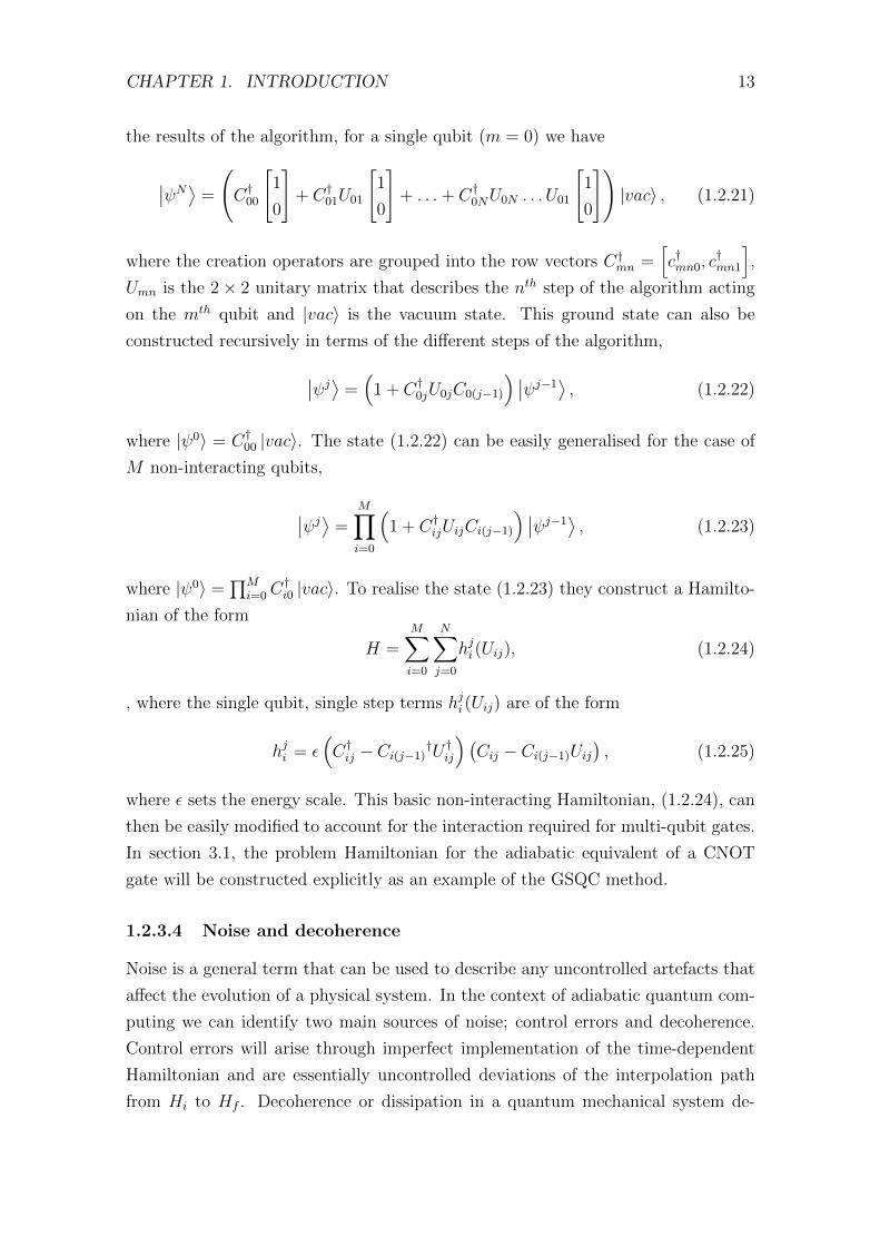
the results of the algorithm, for a single qubit (m = 0) we have
∣∣ψN⟩ =
(C†00
[1
0
]+ C†01U01
[1
0
]+ . . .+ C†0NU0N . . . U01
[1
0
])|vac〉 , (1.2.21)
where the creation operators are grouped into the row vectors C†mn =[c†mn0, c
†mn1
],
Umn is the 2× 2 unitary matrix that describes the nth step of the algorithm acting
on the mth qubit and |vac〉 is the vacuum state. This ground state can also be
constructed recursively in terms of the different steps of the algorithm,
∣∣ψj⟩ =(
1 + C†0jU0jC0(j−1)
) ∣∣ψj−1⟩ , (1.2.22)
where |ψ0〉 = C†00 |vac〉. The state (1.2.22) can be easily generalised for the case of
M non-interacting qubits,
∣∣ψj⟩ =M∏i=0
(1 + C†ijUijCi(j−1)
) ∣∣ψj−1⟩ , (1.2.23)
where |ψ0〉 =∏M
i=0C†i0 |vac〉. To realise the state (1.2.23) they construct a Hamilto-
nian of the form
H =M∑i=0
N∑j=0
hji (Uij), (1.2.24)
, where the single qubit, single step terms hji (Uij) are of the form
hji = ε(C†ij − Ci(j−1)†U
†ij
) (Cij − Ci(j−1)Uij
), (1.2.25)
where ε sets the energy scale. This basic non-interacting Hamiltonian, (1.2.24), can
then be easily modified to account for the interaction required for multi-qubit gates.
In section 3.1, the problem Hamiltonian for the adiabatic equivalent of a CNOT
gate will be constructed explicitly as an example of the GSQC method.
1.2.3.4 Noise and decoherence
Noise is a general term that can be used to describe any uncontrolled artefacts that
affect the evolution of a physical system. In the context of adiabatic quantum com-
puting we can identify two main sources of noise; control errors and decoherence.
Control errors will arise through imperfect implementation of the time-dependent
Hamiltonian and are essentially uncontrolled deviations of the interpolation path
from Hi to Hf . Decoherence or dissipation in a quantum mechanical system de-

CHAPTER 1. INTRODUCTION 14
scribes the quantum noise processes caused by the interaction of the system with
its environment. In practice all quantum systems are open, as it is impossible to
perfectly isolate one from its environment. This interaction of a quantum system
with its environment leads to non-unitary, irreversible evolution of the system as
they become entangled with each other and the system of interest therefore evolves
into a mixed state. The effects of dissipation can be separated into two distinct
types of process in a given basis of orthogonal eigenstates:
• Relaxation or state-mixing: When the Bloch vector describing the state
of the system diffuses in the latitude direction, e.g. parallel to the z-axis of
the Bloch sphere.
• Dephasing or decoherence (when used in its narrower meaning):
When the Bloch vector diffuses in the longitude direction, e.g. the x-y plane
of the Bloch sphere.
It is possible to make a number of intuitive arguments that suggest AQC will be
intrinsically more resistant to the effects of noise than the gate model of quantum
computing. We can first say that for the types of optimisation and search algorithms
that AQC is applied to the phase of the ground state will have no effect on the
result, therefore we can assume pure dephasing is not an issue. By evolving the
system adiabatically slowly we aim to keep it in the ground state at all times, this
will automatically protect it against the effects of relaxation. Also, by keeping the
system at low temperatures where kBT < ∆01 we can try to control the effect of
interactions with the environment that cause transitions between eigenstates.
The natural fault tolerance of AQC was first studied by Childs, Farhi and Preskill
in [7]. They numerically studied the effects of decoherence and unitary control errors
on the adiabatic algorithm for the exact cover problem. They found that neither
of the different types of error had a significant effect on the scaling of the success
probability as a function of the computation time for the relatively small problem
instances (n ≤ 4 bits in the case of decoherence) they could simulate efficiently.
These conclusions were later verified by more analytical means in the papers of
Roland and Cerf: [9], and Ashhab et al.: [8].
A lot of analyses of the performance of AQC tend to neglect the effects of noise
from their models because of AQC’s apparent natural fault tolerance. However,
some results have suggested that noise may play a subtle but important role in the
performance of adiabatic quantum algorithms. Childs et al. noted that in some cases
a unitary control error could increase the success probability of the computation by
providing an alternate interpolation path between Hi and Hf . They also noted that
relaxation caused by interaction with a low temperature environment can help keep

CHAPTER 1. INTRODUCTION 15
the system in the ground state and therefore also improve the success probability.
A paper by Amin, Love and Truncik, [12], explored the idea that in some situations
decoherence can enhance the performance of AQC in more detail. They showed that
thermal mixing around the minimum ground state gap as well as relaxation after
the avoided crossing could help improve performance.
1.2.3.5 Physical realisations
Adiabatic quantum computation was first demonstrated experimentally using nu-
clear magnetic resonance (NMR) by Steffen et al. in 2003 in[26]. They solved a
three qubit instance of the NP-complete MAXCUT optimisation algorithm and
showed that the results were in agreement with the predictions of a simple theo-
retical model that included decoherence. In NMR quantum computing, the nuclear
spins of specific individual atoms in large molecules are identified and used as qubits.
The molecules as a whole therefore represent individual quantum computers. Algo-
rithms can then be implemented by performing operations on an ensemble of these
molecular quantum computers using RF pulses that address the specific spins that
represent qubits. NMR spectroscopy can then be used to readout the ensemble av-
erage of the solution state. Unfortunately, NMR implementations are not scalable
because of the exponential decrease of the signal-to-noise ratio with the system size
[27]. However, these results provided a good experimental proof of principle for
AQC.
Currently, superconducting flux qubits are widely considered to be among the
most promising candidates for the experimental implementation of an AQC system.
These devices consist of small loops of superconducting metal interrupted by a num-
ber of weak links, which are known as Josephson junctions, as shown schematically
in Fig. 1.2.2(a). They are designed such that when the loop is threaded by an
external magnetic field, a persistent current will flow around the loop. The com-
putational basis states are then defined as clockwise and anti-clockwise circulating
currents. This device can be thought of as a double well potential with respect to the
applied flux where the left and right hand wells correspond to the clockwise or anti-
clockwise circulating currents that represent the computational basis states. This
type of qubit can be readily coupled together and controlled inductively and readout
can be performed by probing one of the qubit’s macroscopic quantum variables; the
circulating current ([28]), the flux within the loop ([29]) or the phase ([30]). These
devices also have the advantage that they can be produced using similar fabrication
techniques to those commonly used in the micro-electronics industry, which bodes
well for the scalability. It is also possible to realise a degree of controllability over

CHAPTER 1. INTRODUCTION 16
(a) (b)
Figure 1.2.2: (a) shows a schematic of a single persistent current qubit of the Delfttype [32]. (b) shows the micrograph of a device consisting of three inductivelycoupled flux qubits in resonant tank readout circuit, reproduced from [33].
the inductive coupling elements which is required by the fourth DiVincenzo criterion
for universal quantum computation [31].
This leaves us with the crucial third DiVincenzo criterion to consider; long de-
coherence times. By operating flux qubits at low temperatures they gain a degree
of inherent protection against the effects of noise, as we can assume that the gap
between the two lowest energy states (∆01) will be much larger than kBT , therefore
suppressing thermal excitation. The main sources of noise in flux qubit systems are
therefore background magnetic fluctuations. These can be caused by impurities and
defects in the substrate and superconducting wires, as well as circuit elements like
control lines, coupling devices and readout probes. A number of systematic studies
of the noise in flux qubits have found it to be characterised by a low frequency 1/f
or coloured noise spectrum [34, 35]. Flux qubits with a decoherence time of the or-
der of 10−5s have been demonstrated, e.g. [36], but the question of whether a large
number of them can remain quantum coherent long enough for an AQC operation
to be performed remains open. Despite this, there have been a number of promising
experimental results with flux qubit systems.
In 2006, van der Ploeg et al. demonstrated a system of three coupled flux
qubits that could be used to encode a realisation of the MAXCUT problem in
[33], as shown in Fig. 1.2.2(b). They then made use of a resonant tank circuit
to measure the ground state susceptibility, it was then shown that this could be
used to construct the ground state flux diagram and therefore the solution to the
MAXCUT problem. These results demonstrated a number of the key elements
needed to build an AQC system using flux qubits. Recently, in [37] D-Wave Systems

CHAPTER 1. INTRODUCTION 17
Inc. demonstrated a device consisting of 8 flux qubits with programmable couplings
that can be used to solve adiabatic quantum algorithms which can be described by
an Ising model problem Hamiltonian. They show that the results of an example
computation are in agreement with an explicitly quantum mechanical theoretical
model as oposed to a classical description of the system. Although this device is
limited to solving a certain class of problems it represents an important step in the
process of implementing a practical, large scale AQC system.
1.3 Eigenvalue dynamics
In the field of quantum chaos, which involves the study of the quantum mechanics
of classically chaotic systems, a lot of information about the nature of a system can
be determined by the analysis of the distribution of its energy spectrum. In a lot of
the spectroscopic experiments used to measure this distribution, the energy levels
are determined as a function of some external parameter, e.g. the distribution of the
energy levels of a hydrogen atom in the presence of a strong magnetic field gradually
become chaotic as the strength of the perturbing field is increased. Motivated by
this, in [38] Pechukas derived a set of equations motion for the dynamics of the
energy eigenvalues of a quantum system with a Hamiltonian of the form
H(λ(t)) = H0 + λ(t)V, (1.3.1)
where H0 is the Hamiltonian of the unperturbed system, V is the perturbation
and the perturbation strength λ(t) plays the role of “time” in the system. In [39],
Yukawa simplified Pechukas’s equations of motion to the form
∂
∂λxn =vn,
∂
∂λvn =
∑k 6=n
2 |lnk|2
(xn − xk)3, (1.3.2)
∂
∂λlnm =
∑k 6=m,n
lnklkm
(1
(xn − xk)2− 1
(xm − xk)2
),
by introducing a new set of dynamical variables, where xn are the instantaneous
energy eigenvalues of the system that obey the standard relation (1.2.5), vn = Vnn
are the diagonal matrix elements of the perturbation, lnm = (xn−xm)Vnm for n 6= m
and Vnm are the off-diagonal matrix elements of the perturbation. This system
of equations motion (1.3.2) is now known as the Pechukas-Yukawa model. These
equations of motion are analogous to those of a classical one-dimensional gas with

CHAPTER 1. INTRODUCTION 18
cubic repulsion where the xn take the role of the positions of the gas particles, the
vn their velocity or momenta and the lnm represent the strength of the interaction
between particles n and m. In fact, as no assumptions or simplifications are made
in the derivation of (1.3.2), the mapping of the dynamics of the eigenvalues of the
quantum system to those of the classical 1D gas is exact. The initial conditions
for the Pechukas gas will contain all the information about the Hamiltonian of the
quantum system, (1.3.1), and this simple, generic form of Hamiltonian can be used
to describe a wide range of physical systems.
In [40] Zagoskin, Savel’ev and Nori used the Pechukas-Yukawa equations to
model an adiabatic quantum computer. The Hamiltonian (1.3.1) can be used to
describe the operation of an adiabatic quantum computer by assuming the per-
turbation takes the form of a large bias, i.e. V = ZHb where Z � 1, and that
Hi = H(λ = 1) = H0 + ZHb has a unique and easily achievable ground state. In
this case the final Hamiltonian that encodes the algorithm will take the form of the
unperturbed Hamiltonian, i.e. Hf = H(λ = 0) = H0. This scheme is sometimes
referred to as “quantum annealing” (see [41]) because the perturbation term in the
Hamiltonian (V ) plays a similar role to the “temperature” in simulated annealing
(i.e. it is a source of disorder that is gradually reduced to try to find a desired
ground state), however it is essentially the same as the linear interpolation scheme
of (1.2.13). Using an eigenvalue dynamics approach to model an adiabatic quantum
computer is a particularly relevant and insightful method because knowledge of how
the energy spectrum evolves as a function of time can provide a lot of information
about the performance of the algorithm. For example, the minimum ground state
energy gap width can be easily extracted. Also, being able to identify and analyse
the distribution of avoided crossings between pairs of adjacent energy levels in the
spectrum is advantageous because of Landau-Zener-Stuckelberg tunneling. Landau-
Zener-Stuckelberg tunneling ([42, 43, 44]) is a mechanism by which there exists a
finite probability of tunneling between the states of a quantum system as it moves
through an avoided level crossing at a finite rate and in the absence of noise it
is the sole factor that determines the success probability of an adiabatic quantum
algorithm.
1.4 Random matrices
Random matrix theory was originally developed in the 1950’s by Wigner as a way of
trying to describe the energy spectra of complex nuclei and it has more recently been
successfully applied in the field of quantum chaos. The main principle of random
matrix theory is that the Hamiltonian is thought of as a large matrix with randomly

CHAPTER 1. INTRODUCTION 19
distributed elements which belongs to a large class or ensemble of matrices that
have similar general properties and symmetries, i.e. that it is the properties of the
matrix as a whole and not individual elements that determine the trends in the
corresponding eigenspectrum. The individual matrix elements are often assumed
to obey Gaussian distributions, which allows the definition of the three ensembles;
the Gaussian orthogonal ensemble (GOE), the Gaussian unitary ensemble (GUE)
and the Gaussian symplectic ensemble (GSE). These three ensembles are defined by
the type of transformation the constituent matrices are invariant under and there
properties are summarized in the table 1.1 ([45, 46]).
GOE GUE GSETime-reversal symmetry Yes No Yes
Spin-1/2 interaction No n/a YesMatrix elements real complex real-quaternionic
Transformation invariance orthogonal unitary symplectic
Table 1.1: Summary of the properties and symmetries of the three Gaussian ensem-bles of random matrix theory [45, 46].
Throughout this work we will only be concerned with the GOE and GUE. They
will be useful as a means of modeling different types of generic Hamiltonians. The
probability distribution functions for the matrix elements of N×N random matrices
drawn from the GOE and GUE are
p(H11, . . . , HNN) =
(A
π
)N/2(2A
π
)N(N−1)/2
exp
(−A
∑n,m
H2nm
)and (1.4.1)
p(H11, . . . , HNN) =
(A
π
)N/2(2A
π
)N(N−1)
exp
(−A
∑n,m
[(Re(Hnm))2 + (Im(Hnm))2
)](1.4.2)
respectively ([45, 46]), where A is determined by the variances 〈H2nn〉 = 1/2A and
〈H2nm〉 = 1/4A. An interesting property of the Gaussian ensembles is that in all
three cases the average density of states is described by Wigner’s semicircle law;
which is of the form
〈ρ(E)〉 =
Aπ
√2NA− E2, for |E| <
√2NA
0, for |E| >√
2NA
(1.4.3)
([45, 46]).
In the papers [17] and [18] the authors attempted to determine whether the
statistical properties of the energy spectra of adiabatic quantum computers can

CHAPTER 1. INTRODUCTION 20
be described using the predictions of random matrix theory and hence discover
whether it is applicable to use random matrix theory to predict the behaviour of
AQC for large problem instances. In general they found that for problem instances
of increasing complexity the degree of regularity of the spectrum decreased meaning
random matrix theory becomes more applicable. In particular, the bulk of the
eigenspectrum (i.e. eigenstates from the centre of the spectrum) appear to be well
described by random matrix theory. Whereas the properties of the top and bottom
parts of the energy spectrum, the latter of which is of critical importance in AQC,
do not appear to fit the predictions of random matrix theory quite as well, meaning
it may not be applicable in those regions. Another way in which random matrices
have been used in the study of adiabatic quantum computing is as a simple way of
representing noise in the Hamiltonian; this was done by Roland and Cerf in [9].

Chapter 2
Generalised Pechukas-Yukawa
model
2.1 Generalised Pechukas-Yukawa equations
As mentioned in section 1.3 the Pechukas-Yukawa model offers a method of exploring
the dynamics of the energy eigenvalues of a quantum system. This model is partic-
ularly appropriate for studying an adiabatic quantum computer as it is based on a
Hamiltonian of a similar form and knowledge about the behaviour of the lowest few
energy levels is crucial when analysing the performance of adiabatic quantum algo-
rithms. We aim to explore the effects of noise on an adiabatic quantum computer,
therefore we need to generalise the Pechukas-Yukawa equations to the stochastic
case. This can be done by including an additional term in the Hamiltonian, δh(λ),
which accounts for the effects of noise on the system. At this point we need not
make any assumptions about the exact form of the stochastic variable δh(λ). We
follow the derivation of the standard Pechukas-Yukawa equations described in [46],
except that we start with the following Hamiltonian;
H(λ(t)) = H0 + λ(t)V + δh(λ(t)) (2.1.1)
where the perturbation strength λ(t) is interpreted as ‘time’.
The instantaneous eigenvalues of H(λ) are denoted by xn(λ) and the correspond-
ing eigenfunctions by |n(λ)〉;
H(λ) |n(λ)〉 = xn(λ) |n(λ)〉 . (2.1.2)
21

CHAPTER 2. GENERALISED PECHUKAS-YUKAWA MODEL 22
The eigenfunctions obey the orthogonality relation
〈n|m〉 = δnm, (2.1.3)
which after differentiation with respect to ‘time’ (λ) gives(∂
∂λ〈n|)|m〉+ 〈n|
(∂
∂λ|m〉)
= 0. (2.1.4)
If we now introduce the operator
H = i∂
∂λ, (2.1.5)
with matrix elements
Hnm = 〈n|H |m〉 , (2.1.6)
which allows (2.1.4) to be written as Hnm = H∗mn, i.e. H is hermitian.
We can now derive an equation for the ‘time’ evolution of the matrix elements
of an arbitrary operator A
d
dλ〈n|A |m〉 =
(∂
∂λ〈n|)A |m〉+ 〈n| ∂A
∂λ|m〉+ 〈n|A
(∂
∂λ|m〉), (2.1.7)
using the completeness relation,∑
k |k〉 〈k| = 1, we get
d
dλ〈n|A |m〉 =
∑k
[(∂
∂λ〈n|)|k〉 〈k|A |m〉+ 〈n|A |k〉 〈k|
(∂
∂λ|m〉)]
+〈n| ∂A∂λ|m〉 .
(2.1.8)
Using the definition (2.1.5) we have
dAnmdλ
= i∑k
(HnkAkm − AnkHkm) +
(∂A
∂λ
)nm
, (2.1.9)
which, when written in matrix notation and H is interpreted as a Hamiltonian, is
simply the equation of motion for an operator A in the Heisenberg picture
dA
dλ= i[H,A] +
∂A
∂λ. (2.1.10)
If we insert the Hamiltonian H(λ) for A in (2.1.9) we have
xnδnm = iHnm(xm − xn) + Vnm + ˙δhnm, (2.1.11)
where the dot denotes differentiation with respect to ‘time’ and ˙δhnm is the instan-

CHAPTER 2. GENERALISED PECHUKAS-YUKAWA MODEL 23
taneous ‘time’ derivative of an element of the noise matrix, which arises from the
partial derivative term of (2.1.9). For n = m (2.1.11) gives
xn = Vnn + ˙δhnn (2.1.12)
and for n 6= m it gives
Hnm =Vnm + ˙δhnmi(xn − xm)
. (2.1.13)
Next we insert V for A in (2.1.9) to get
Vnm = i∑k
(HnkVkm − VnkHkm) . (2.1.14)
For n = m in (2.1.14), using (2.1.13), we obtain
Vnn =∑k 6=n
(Vnk + ˙δhnk
)Vkn
xn − xk−Vnk
(Vkn + ˙δhkn
)xk − xn
(2.1.15)
=∑k 6=n
2VnkVkn + ˙δhnkVkn + Vnk ˙δhknxn − xk
(2.1.16)
as for k = n the contribution to the sum is HnnVnn − VnnHnn = 0. For n 6= m in
(2.1.14) we get
Vnm =∑k 6=n,m
(Vnk + ˙δhnk
)Vkm
xn − xk−Vnk
(Vkm + ˙δhkm
)xk − xm
+ i(HnnVnm − VnnHnm) + i(HnmVmm − VnmHmm) (2.1.17)
where the second and third terms are the contributions to the sum for k = n and
k = m respectively. This can be rearranged to give
Vnm =∑k 6=n,m
[VnkVkm + ˙δhnkVkm
xn − xk+VnkVkm + Vnk ˙δhkm
xm − xk
]+ i(Hnn −Hmm)Vnm + iHnm(Vmm − Vnn). (2.1.18)
The second term can be removed by the substitution
Vnm = Vnm exp
[i
∫(Hnn −Hmm)dt
]. (2.1.19)

CHAPTER 2. GENERALISED PECHUKAS-YUKAWA MODEL 24
as the Vnm obey the same equation of motion as the Vnm but without the second
term of (2.1.18); therefore we may assume that Hnn = 0 and write Vnm instead of
Vnm without loss of generality. Using the identity (2.1.13), the third term in (2.1.18)
can then be rearranged to give
Vnm =∑k 6=n,m
[VnkVkm + ˙δhnkVkm
xn − xk+VnkVkm + Vnk ˙δhkm
xm − xk
]
− (Vnm + ˙δhnm)(Vnn − Vmm)
xn − xm(2.1.20)
Vnm =∑k 6=n,m
[VnkVkm + ˙δhnkVkm
xn − xk+VnkVkm + Vnk ˙δhkm
xm − xk
]
− Vnm(Vnn − Vmm)
xn − xm−
˙δhnm(Vnn − Vmm)
xn − xm. (2.1.21)
Equations (2.1.12), (2.1.16) and (2.1.21) form a closed system of equations de-
scribing the dynamics of the energy eigenvalues of H(λ), similar to those originally
derived by Pechukas in [38].
We can now introduce the new dynamical variables vn and lmn as done by Yukawa
in [39].
vn = Vnn (2.1.22)
lnm = (xn − xm)Vnm, n 6= m (2.1.23)
If we imagine that the energy eigenvalues xn take the role of the position of the nth
particle in a 1D classical gas, the new variables vn and lmn are analogous to the
particle’s velocity and the particle-particle repulsion strength respectively. The new
variables vn and lmn can be substituted into equations (2.1.12), (2.1.16) and (2.1.21)
to derive a system of equations describing the dynamics of the 1D classical gas.
Substituting (2.1.22) into (2.1.12) gives the equation of motion for the nth particle’s
position
xn = vn + ˙δhnn. (2.1.24)
Substitution of (2.1.23) into (2.1.16) gives the equation of motion for the nth parti-
cle’s velocity
vn =∑k 6=n
[2lnklkn
(xn − xk)2(xk − xn)+
˙δhnklkn(xn − xk)(xk − xn)
+lnk ˙δhkn
(xn − xk)2
], (2.1.25)

CHAPTER 2. GENERALISED PECHUKAS-YUKAWA MODEL 25
as V is a hermitian matrix lnk = −l∗kn for k 6= n, therefore we can write
vn =∑k 6=n
[2 |lnk|2
(xn − xk)3+lnk ˙δhkn − ˙δhnklkn
(xn − xk)2
]. (2.1.26)
If we then differentiate (2.1.23) with respect to ‘time’;
lnm =d
dλ(xnVnm − xmVnm) (2.1.27)
= (xnVnm + xnVnm)− (xmVnm + xmVnm) (2.1.28)
= Vnm(xn − xm) + Vnm(xn − xm). (2.1.29)
Then equation (2.1.24) and the identities (2.1.22) and (2.1.23) can be substituted
into give;
lnm = Vnm(xn − xm) +lnm(vn − vm)
(xn − xm)+lnm( ˙δhnn − ˙δhmm)
(xn − xm). (2.1.30)
The new variable lnm can then be substituted into (2.1.21);
Vnm =∑k 6=n,m
[lnklkm
(xn − xk)2(xk − xm)− lnklkm
(xm − xk)2(xn − xk)+
˙δhnklkm(xn − xk)(xk − xm)
+lnk ˙δhkm
(xn − xk)(xm − xk)
]+lnm(vm − vn)
(xn − xm)2+
˙δhnm(vm − vn)
(xn − xm)(2.1.31)
Combining equations (2.1.30) and (2.1.31) we derive an equation of motion for the
particle-particle repulsion strength in the eigenvalue gas (N.B. the second term in
(2.1.30) will cancel the first term outside the sum in (2.1.31)),
lnm = (xn − xm)∑k 6=m,n
[lnklkm
(1
(xn − xk)2(xk − xm)− 1
(xm − xk)2(xn − xk)
)
+lnk ˙δhkm − lkm ˙δhnk(xm − xk)(xn − xk)
]+ ˙δhnm(vm − vn) +
lnm( ˙δhnn − ˙δhmm)
(xn − xm). (2.1.32)
The (xn − xm) can then be taken inside the sum to give
lnm =∑k 6=m,n
[lnklkm
(1
(xn − xk)2− 1
(xm − xk)2
)+
(xn − xm)(lnk ˙δhkm − lkm ˙δhnk)
(xm − xk)(xn − xk)
]
+ ˙δhnm(vm − vn) +lnm( ˙δhnn − ˙δhmm)
(xn − xm). (2.1.33)

CHAPTER 2. GENERALISED PECHUKAS-YUKAWA MODEL 26
We now have the following dynamical equation system to describe the motion of
the energy eigenvalues of the Hamiltonian H(λ(t)) = H0 + λ(t)V + δh(λ(t));
xn =vn + ˙δhnn,
vn =∑k 6=n
[2 |lnk|2
(xn − xk)3+lnk ˙δhkn − ˙δhnklkn
(xn − xk)2
], (2.1.34)
lnm =∑k 6=m,n
[lnklkm
(1
(xn − xk)2− 1
(xm − xk)2
)+
(xn − xm)(lnk ˙δhkm − lkm ˙δhnk)
(xm − xk)(xn − xk)
]
+ ˙δhnm(vm − vn) +lnm( ˙δhnn − ˙δhmm)
(xn − xm).
When the noise term δh(λ) equals zero at all times this simply reduces to the normal
Pechukas-Yukawa system as expected.
We have derived a generalised stochastic form of the Pechukas-Yukawa model of
eigenvalue dynamics. This retains the key feature of the standard Pechukas-Yukawa
equations as it is also an exact mapping of the quantum eigenvalue dynamics to a
classical gas. It is also done without making any assumptions about the nature of
the noise source δh(λ) and can therefore be used to model a wide range of different
physical systems.
2.2 Random matrix Noise model
In order to close the generalised Pechukas-Yukawa system of dynamical equations
(2.1.34) we need to consider the exact nature of the noise term δh(λ). In reality,
noise in most physical systems arises from a number of different sources via different
mechanisms, because of this it seems reasonable to assume that, by the central limit
theorem, the sum of their effects will be a random term in the Hamiltonian with
independent Gaussian distributed elements. Therefore, we take the noise term δh(λ)
to be a random matrix drawn from the Gaussian ensembles of random matrix theory
described in section 1.4; this is similar to the noise model used in [9].
The generalised Pechukas-Yukawa model depends on the derivative of the noise
term, ˙δh(λ), because of this we require a noise source which obeys a simple stochastic
differential equation. As mentioned in section 1.2.3.5, some of the most promising
physical realisations of adiabatic quantum computers are built using superconduct-
ing qubits and the noise observed in these types of devices has a coloured (non-flat)
frequency spectral density [34]. Therefore, we will assume that the elements of the
noise matrix evolve in time according to a simple stationary stochastic process which

CHAPTER 2. GENERALISED PECHUKAS-YUKAWA MODEL 27
has a coloured spectral density, the Ornstein-Uhlenbeck process [47];
˙δhij(λ) = −τδhij(λ) + εηij(λ) (2.2.1)
where τ is the correlation time, ε is the noise amplitude and η(λ) is a random
matrix valued function with 〈η(λ)〉 = 0 and 〈η(λ)η(λ′)〉 = δ(λ − λ′), i.e. a white
noise process.
2.3 Numerical methods and testing
As an initial test of the generalised Pechukas-Yukawa model, a simple simulation
that numerically solved the equations (2.1.34) with the random matrix noise model
was developed in MATLAB. We assume that the perturbation takes the form of a
large bias, i.e. V = ZHb where Z � 1. The problem (Hf = H0) and bias (Hb)
Hamiltonians are taken to be random matrices drawn from the Gaussian unitary
ensemble. The noise term (δh(λ)) is taken as a random matrix drawn from the
Gaussian orthogonal ensemble and is assumed to evolve in time according to equation
(2.2.1).
The system of equations (2.1.34) is complex and the noise term will fluctuate
on a relatively fast time scale compared to the trajectories of the eigenvalues, be-
cause of this the stability of the numerical methods that are used is an important
consideration. Multistep methods, such as the Adams-Moulton predictor corrector,
are particularly stable as they use data from a number of the preceding points to
compute the next point [48]. This is in comparison to single-step methods, like the
Runge-Kutta method, which only use data from the previous point in the calculation.
The Adams-Moulton method essentially works by fitting a cubic polynomial through
the last n (which defines the order of the method) data points and then calculating
a rough approximation of the integral from the current point to the next; this is the
predictor step. The results from the predictor step are then used in the corrector
formula to calculate a more accurate value of the integral at the next data point.
The Adams-Moulton method requires the first n data points to be calculated using
a single-step method. In the simulation a variable order Adams-Moulton method is
used to solve (2.1.34) and a simple 2nd order Runge-Kutta method is used to solve
(2.2.1). We also attempt to improve numerical accuracy by using a finer time step
towards the end of the computation, because the Pechukas gas will contract as the
large bias Hamiltonian is turned off and we therefore expect the majority of level
and avoided crossings to occur when λ(t) & 0.
Figure 2.3.2 shows an example of the energy spectrum of a 4-qubit system calcu-

CHAPTER 2. GENERALISED PECHUKAS-YUKAWA MODEL 28
lated using the generalised Pechukas-Yukawa model derived in section 2.1. A noise
amplitude of ε = 0.1, a large bias strength of Z = 10 and a short correlation time
of τ = 0.1 were used; the magnitude of these values will be typical of those used
throughout the rest of this work. The results are compared to those found by direct
diagonalization of H(t) at a number of points in time and it is found that they agree
to approximately 3 decimal places which corresponds to a relative error of less than
0.5%, indicating the accuracy of the numerical methods used.
Knowledge of how the energy spectrum of an adiabatic quantum computer
evolves over time allows the identification of the critical points in the computa-
tion process. Namely, any avoided or level crossings, as at these points there will
be a finite probability of the system tunneling out of its current state. The main
tunneling mechanism at these critical points will be Landau-Zener-Stuckelberg tun-
neling ([42, 43, 44]) and the probability of excitation from |m〉 to |m+ 1〉 via this
mechanism is given by;
PLZS = exp
− ∆2m,m+1
|〈m|ZHb |m+ 1〉|∣∣∣λ∣∣∣ , (2.3.1)
where ∆m,m+1 is the minimum separation between levels xm and xm+1, as shown in
Fig. 2.3.1, and |λ| is the computation speed. Unless stated otherwise, we will always
assume that system undergoes uniform evolution, therefore |λ| = 1T
, where T is the
computation time. These critical points can be readily found by searching for the
minima of |xm(λ)− xm+1(λ)|. Then the sequence of critical points in the spectrum
that can lead to excitation out of the ground state can be identified. By applying
equation (2.3.1) at these points it is possible to calculate how the level occupation
changes over time and hence find the success probability of the computation. This
method yields a tree-like structure with branches between adjacent levels at avoided
crossings; the probability of occupation can then be visualised as diffusing across this
tree structure. The algorithm used to perform this analysis is shown in Fig. 2.3.3
and copy of the MATLAB code is listed in appendix A. A two-state approximation
is often used when looking at an AQC operation, e.g. as in [12], this assumes that
the minimum gap between the ground and first excited states is the limiting factor
for transitions out of the ground state. The algorithm for estimating occupation
described here can be viewed as a natural extension of the two-state approximation.

CHAPTER 2. GENERALISED PECHUKAS-YUKAWA MODEL 29
Figure 2.3.1: Example showing a critical point in the energy spectrum of an adiabaticquantum computer, namely an avoided crossing between the ground and first excitedstate. The minimum gap at this point is denoted ∆min.

CHAPTER 2. GENERALISED PECHUKAS-YUKAWA MODEL 30
(a) Energy spectrum over time
(b) Relative error
Figure 2.3.2: Plots showing a comparison of the energy spectrum calculated usingthe generalised Pechukas-Yukawa model and the results of direct diagonalisation(crosses) for a 4-qubit system with GUE Hamiltonians and GOE random matrixnoise where Z = 10, ε = 0.1 and τ = 0.1.

CHAPTER 2. GENERALISED PECHUKAS-YUKAWA MODEL 31
Figure 2.3.3: Flowchart describing algorithm used to estimate the occupation prob-abilities as a function of time for a given energy spectrum based on analysis of thecritical points.

Chapter 3
The CNOT gate
3.1 The CNOT problem Hamiltonian
As an example of a prototypical quantum algorithm, we will study the adiabatic
equivalent of the CNOT gate. This can be constructed using the GSQC method
described in 1.2.3.3. The CNOT gate is a two qubit gate which in conjuction with
single qubit roatations forms one of the simplest sets of universal quantum gates. In
this family of universal gates the inter-qubit action of the CNOT gate is necessary
to generate the entanglement that is required for quantum computation, because of
this it is a fundamental building block in quantum circuits.
As described in section 1.2.3.3, we can construct a problem Hamiltonian using
the GSQC method by visualising each qubit as an array of quantum dots that share
a single spin polarised electron. A single CNOT gate is a 1 step, 2 qubit algorithm so
we require an array of 8 quantum dots (effectively 4 physical qubits) for the GSQC
version, this system is shown schematically in Fig. 3.1.1. The CNOT gate will flip
the state of the target qubit (m = 1) if the state of the control qubit (m = 0) is in
state 1, therefore we require an identity operator to be applied to m = 1 if m = 0 is
in the state 0 and if m = 0 is in 1 we need a NOT gate to be applied to m = 1. The
single qubit NOT operation is simply described by the well known Pauli matrix σx.
The multi-qubit recursion relation for the solution state, (1.2.23), for this operation
can be written as
∣∣ψ1⟩
=(I + c†010c000C
†11IC10 + c†011c001C
†11σxC10
) ∣∣ψ0⟩, (3.1.1)
where the 2nd and 3rd terms in the brackets apply the identity and NOT operations
respectively in the relevant situations. The Hamiltonian for this operation takes the
32

CHAPTER 3. THE CNOT GATE 33
form;
HCNOT =(c†010C
†11 − c
†000C
†10
)(C11c010 − C10c000)
+(c†011C
†11 − c
†001C
†10σx
)(C11c011 − σxC10c001)
+ C†00C00C†11C11 + C†01C01C
†10C10, (3.1.2)
where the first and second terms are modifications of the single qubit, single step
terms in (1.2.24) that apply identity and NOT operations respectively in the relevant
situations. The third term in (3.1.2) is required to penalise states in which one qubit
has gone through the CNOT gate without the other.
Figure 3.1.1: Schematic of the quantum dot array used to encode a CNOT gate intoHamiltonian form using the GSQC method.
In order to write the Hamiltonian (3.1.2) explicitly we need to define the fermionic
creation and annihilation operators explicitly. The theoretical arrays of quantum
dots used to represent a single qubit have a basis of 5 possible states, the vacuum
state plus the electron occupying each dot in turn, which we describe with the
following basis vectors in a 5D Hilbert space;
|vac〉 =
1
0
0
0
0
, |m00〉 =
0
1
0
0
0
. . . |m11〉 =
0
0
0
0
1
(3.1.3)

CHAPTER 3. THE CNOT GATE 34
We know that the fermionic creation operators must satisfy the following relations;
C†m00 |vac〉 = |m00〉 , C†m01 |vac〉 = |m01〉 , C†m10 |vac〉 = |m10〉 , C†m11 |vac〉 = |m11〉
and{Ci, C
†j
}= δij, (3.1.4)
and from these relations it is straightforward to write 5× 5 matrices that perform
the desired operation, e.g.
c†m00 =
0 0 0 0 0
1 0 0 0 0
0 0 0 0 0
0 0 0 0 0
0 0 0 0 0
0 0 0 0 0
. (3.1.5)
The creation operators for the M = 2 qubit system of the CNOT gate are then
constructed by taking the tensor product with the identity operator, e.g.
C†000 = C†00 ⊗ I and C†100 = I ⊗ C†00. (3.1.6)
Using equation (3.1.2) we can then construct the CNOT Hamiltonian in the 25D
composite Hilbert space, this can then be truncated to the required 16D ((2 (N + 1))M
where M = 2 qubits and N = 1 steps) Hilbert space by tracing out the vacuum
state.
3.2 Initial conditions
The ground state energy of a GSQC Hamiltonian, such as HCNOT (3.1.2), is iden-
tically 0 by design [11]. To ensure that we arrive at the desired solution state, as
opposed to a state that appears correct but corresponds to starting in a different
initial state, it is necessary to add a perturbation to the Hamiltonian defining the
initial state, Hinput. This perturbation ensures that states corresponding to un-
desired inputs are pushed well above the low-lying states that play a role in the
computation. If we assume that the our system begins in one of the computational
basis states, the CNOT gate has four possible operations. These four operations
and the appropriate perturbations that define their initial states are shown in Table
3.1, where the constant µ simply sets the energy scale.
As mentioned in section 1.3 all the information about the form of the problem
Hamiltonian (Hf = H0 = HCNOT + Hinput) is encoded in the initial conditions of

CHAPTER 3. THE CNOT GATE 35
IN OUT Hinput
|00〉 |00〉 −µ(c†000c000 + c†100c100
)|01〉 |01〉 −µ
(c†000c000 + c†101c101
)|10〉 |11〉 −µ
(c†001c001 + c†100c100
)|11〉 |10〉 −µ
(c†001c001 + c†101c101
)Table 3.1: The operations of the CNOT gate for the four computational basis statesand their corresponding Hinput. In Hinput, µ sets the energy scale.
the eigenvalue gas (i.e. xn(λ = 1), vn(λ = 1) and lmn(λ = 1)). For the sake of
generality, the initial conditions for the Pechukas gas are calculated using a first
order perturbation theory expansion in terms of Z−1 at λ(t) = 1, where
Hi = H(1) = H0 + ZHb + δh(1) ≡ Z(Hb + Z−1H0 + Z−1δh(1)
). (3.2.1)
For the initial eigenvalue positions, we have
xn(1) = ZHb
∣∣n(0)⟩
+⟨n(0)∣∣ (HCNOT +Hinput)
∣∣n(0)⟩
+⟨n(0)∣∣ δh(1)
∣∣n(0)⟩, (3.2.2)
where we assume that Hb has a nondegenerate, well spaced energy spectrum with
eigenvalues En. Using the definitions (2.1.22) and (2.1.23), this gives
xn(1) = zEn + (HCNOT +Hinput)nn + (δh(1))nn , (3.2.3)
vn(1) = zEn, (3.2.4)
lnm(1) = (En − Em) z((HCNOT +Hinput)nm + (δh(1))nm
). (3.2.5)
This approach should be more representative of a generic implementation of an AQC
system than direct calculation from a specific Hb.
Throughout this work, the initial noise term δh(1) will be a random matrix
drawn from the GOE with amplitude ε. We will take the numerical constants
µ = 0.1, Z−1 = 0.1 and τ = 0.1. We always assume that at λ(t) = 1 the ground
state is occupied with probability 1.

Chapter 4
The energy spectra of the CNOT
gate
The numerical methods discussed in section 2.3 were used to solve the generalised
Pechukas-Yukawa system, (2.1.34), for the example of the CNOT gate, (3.1.2), with
generic initial conditions calculated perturbatively, (3.2.5).
We start by examining the case of an idealised system where there is an absence
of noise, ε = 0.The energy spectra as a function of the perturbation strength or
‘time’ λ(t) for the 4 operations of the CNOT gate are shown in Fig. 4.0.1. Initially,
at λ = 1 we have a well spaced spectrum due to the large bias z, as required in
the AQC scheme. As λ(t) decreases and the perturbation is switched off we see a
contraction of the eigenvalue gas to a densely packed region near λ & 0. At λ = 0,
the system reaches the final state that encodes the results of the computation and
we can see that the xn(0) are in good agreement with the values found by direct
diagonalisation of H(0) = HCNOT +Hinput = H0; This confirms the accuracy of the
numerical methods set out in section 2.3.
The final region, where λ & 0, will be of crucial importance to the success of
computation process, as it is in this region of closely packed levels where avoided and
level crossings between adjacent levels will be found and therefore where tunneling
out of the ground state is most likely to occur. In the idealised noiseless situation
shown in Fig. 4.0.1 there are number of level crossings between adjacent energy
levels in this region in all four spectra. Crucially, in the |01〉 → |01〉, |10〉 →|11〉 and |11〉 → |10〉 operations there are crossings between the ground and first
excited states, which therefore means there is 0 probability of the system being
successfully found in the ground state at λ = 0. These degeneracies correspond to
different solutions of the characteristic equation having the same eigenvalue because
of symmetries in the HamiltonianH(λ). These degeneracies are clearly not desirable
36

CHAPTER 4. THE ENERGY SPECTRA OF THE CNOT GATE 37
in an AQC system as they obstruct the computation process.
The |01〉 → |01〉, |10〉 → |11〉 and |11〉 → |10〉 operations represent examples of
when the usual stipulation that [Hi, Hf ] 6= 0 has not been met. This situation could
be avoided by an alternative choice of initial conditions (Hb) but a suitable choice
may not be so clear if you have a particularly complex problem Hamiltonian or if
there are limitations on the controllability of the system. However, the effects of
noise have not been taken into account yet. The addition of a generic perturbation
to the system should break the symmetries and split the degeneracies; in reality, all
physical systems will be subject to some form of perturbation from noise.
The ‘time’ dependence of the velocities (vn(λ)) and coupling strengths (lmn(λ))
of the eigenvalue gas particles were also investigated. Figure 4.0.2 shows the ‘time’
dependence of vn(λ) for the |00〉 → |00〉 operation in an ideal noise-free system. We
can see that level velocities are constant at the start of the computation process
when the levels are well spaced. As λ(t) → 0 and the eigenvalue gas contracts
the 1/ (xn − xk)3) term in the equation of motion for vn(λ) in (2.1.34) becomes the
dominant term and we see some variation in the velocities of the close packed levels,
although some do remain constant. The inter-particle coupling strengths (lmn(λ))
are all shown to be constant in ‘time’ in Fig. 4.0.3. This arises from the initial
values calculated using (3.2.5), a number of them are equal to 0. We can see that
for the coupling strengths that are initially non-zero there will be no other non-zero
couplings that can contribute to the sum in the equation of motion (2.1.34) and
therefore all lmn(λ) = 0.
We now investigate the effects of the noise model described in section 2.2 on the
dynamics of the eigenvalue gas. Throughout this work, we will consider noise at a
range of different amplitudes (ε); usually ε = 0.025, 0.05, 0.075 and 0.1. We can
see from the equations (2.1.34) that the noise should have a significant effect on the
dynamics as all three equations of motion are strongly dependent on ˙δh(λ). The
effects of the noise should be particularly noticeable as λ(t) is near zero and the
levels become more densely packed, because a number of the noise terms depend on
the inverse of the gaps between levels.
In Fig. 4.0.4 we can see that the main effect of the noise on the energy spectra
is to split all the degeneracies into avoided crossings, as expected. This means there
will always be a finite success probability for all 4 operations of the CNOT gate when
ε > 0. The majority of these avoided crossings are in the densely packed region where
λ & 0 and this is therefore where we expect excitation out of the ground state to
occur. The algorithm described in section 2.3 will be used to analyse the sequences
of crossings in these spectra and estimate the level occupations. It is important
to note that the noise perturbations will drive the xn(0) and therefore |0(λ = 0)〉

CHAPTER 4. THE ENERGY SPECTRA OF THE CNOT GATE 38
Figure 4.0.1: The energy spectra of the 4 possible operations of the adiabatic CNOTgate in the absence of noise. The blue crosses show the results of direct diagonali-sation of the relevant H0 and agree with the evolution of the Pechukas-Yukawa gasto 4 significant figures.

CHAPTER 4. THE ENERGY SPECTRA OF THE CNOT GATE 39
Figure 4.0.2: Plot showing the particle velocities (vn(λ)) for the |00〉 → |00〉 opera-tion of the CNOT gate in the absence of noise.
Figure 4.0.3: Plot showing the non-zero particle-particle coupling strengths (lmn(λ))for the |00〉 → |00〉 operation of the CNOT gate in the absence of noise. All theother coupling strengths for this operation are equal to zero at all times.

CHAPTER 4. THE ENERGY SPECTRA OF THE CNOT GATE 40
away from the ideal solution state. This is clearly an undesirable effect on an AQC
process and it will be considered in greater detail in the following chapter 5.
The effects of a coloured noise source on the ‘time’ dependence of the level
velocities (vn(λ)) and coupling strengths (lmn(λ)) are shown in Fig. 4.0.5 and Fig.
4.0.6 respectively. In both cases, we see rapid fluctuations when λ(t) is close to zero.
This is because the noise terms in the equations of motion become the dominant
terms in the dynamics, as they depend on the rapidly fluctuating ˙δh(λ) and the
inverse of the gaps. The lmn(λ) = 0 in the ideal case now also show some fluctuation
because of the noise term outside the sum in the equation of motion. These results
serve to confirm the fact that noise has a considerable effect on the eigenvalue
dynamics in the last crucially important moments of the computation process.
As mentioned in section 1.4, the applicability of random matrix theory to closed
AQC systems has been studied previously in [17] and [18] by looking at the distri-
butions of gaps in the spectra. We now go on to investigate the effects of noise on
the nearest neighbour spacing statistics. The distribution of the average energy gap,
∆m,m+1, at avoided crossings for each noise realisation of the |00〉 → |00〉 operation
at a range of noise amplitudes is shown in Fig. 4.0.7. The distributions are Gaus-
sian in shape and shifted away from zero, which shows that we have level repulsion
at avoided crossings, as expected. The mean values of the distributions, ∆m,m+1,
appear to generally increase with ε which can be explained by the fact that noise
fluctuations in the trajectories of the energy levels will drive them apart, widening
the gaps.
The minimum gap between the ground and first excited states, ∆01, is often
seen as the limiting factor in AQC and the results of [17] and [18] suggest that it
sometimes shows different behaviour to spacings in the bulk of the spectrum. The
spacing distribution for the gaps at avoided crossings between x0(λ) and x1(λ) for
the |00〉 → |00〉 operation are shown in Fig. 4.0.8(a). The distribution is unimodal
and has an elongated tail reminiscent of the Wigner distributions of random matrix
theory [46]. The mean of the distribution is approximately constant, although we do
see some variation as a result of the noise. We also see a degree of level repulsion as
the distribution has a lack of small spacings and is shifted away from zero gap. This
will be due to the fact that we have intrinsic level repulsion, i.e. we have ∆01 6= 0
when ε = 0.
In the ground state gap distribution for the |01〉 → |01〉 operation, shown in Fig.
4.0.8(b), we have a more Poissonian-like distribution with an abundance of smaller
gaps, which shows a lack of level repulsion. This is because it has a degeneracy
at ε = 0 and it therefore has no intrinsic level repulsion and the non-zero gap is
created by the noise. The mean gap width, ∆01, can be seen to clearly increase
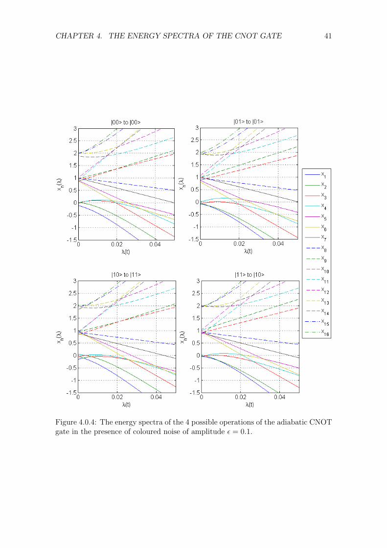
CHAPTER 4. THE ENERGY SPECTRA OF THE CNOT GATE 41
Figure 4.0.4: The energy spectra of the 4 possible operations of the adiabatic CNOTgate in the presence of coloured noise of amplitude ε = 0.1.

CHAPTER 4. THE ENERGY SPECTRA OF THE CNOT GATE 42
Figure 4.0.5: Plot showing the particle velocities (vn(λ)) for the |00〉 → |00〉 opera-tion of the CNOT gate in the presence of coloured noise of amplitude ε = 0.1.
Figure 4.0.6: Plot showing the non-zero particle-particle coupling strengths (lmn(λ))for the |00〉 → |00〉 operation of the CNOT gate in the presence of coloured noise ofamplitude ε = 0.1.

CHAPTER 4. THE ENERGY SPECTRA OF THE CNOT GATE 43
Figure 4.0.7: Plot showing the distributions of average energy gap width (∆m,m+1)at avoided crossings in the energy spectra of each noise realisation for the |00〉 → |00〉operation of the CNOT gate at a range of noise amplitudes. The mean val-ues of the distributions are ∆m,m+1 = 0.1262, 0.1250, 0.1275 and 0.1296 forε = 0.025, 0.05, 0.075 and 0.1 respectively.
proportionally with the noise amplitude. The ground state spacing distributions for
the |10〉 → |11〉 and |11〉 → |10〉 operations are similar to that of the |01〉 → |01〉operation, as they also have no intrinsic level repulsion.
For spacings between states in the bulk of the spectrum we will have some
multimodal distributions as they tend to be involved in a greater number of avoided
crossings. An example of this is shown in Fig. 4.0.9 for ∆45 for the |01〉 → |01〉operation, where we have a Poissonian peak at small spacings and then a Gaussian
peak at larger spacings.
The Brody parameter offers a convenient method of determining whether an
energy spectrum is regular or irregular. If the system’s spectrum is regular we know
that its dynamics are controlled by symmetries and conservation laws; whereas if
they are irregular, the dynamics will be complex and chaotic resulting from a lack of
symmetries. The Brody distribution interpolates from a regular Poissonian nearest
neighbour spacing distribution at q = 0 to an irregular Wigner nearest neighbour
spacing distribution for the GOE at q = 1,
p(s) = (q + 1)aqsqe−aqs
q+1
(4.0.1)

CHAPTER 4. THE ENERGY SPECTRA OF THE CNOT GATE 44
(a) |00〉 → |00〉
(b) |01〉 → |01〉
Figure 4.0.8: Distribution of minimum ground state energy gaps for the |00〉 →|00〉 and |01〉 → |01〉 operations of the CNOT gate at a range of noise am-plitudes. The gap width is renormalised by ∆01/∆01. The mean values ofthe distributions for ε = 0.025, 0.05, 0.075 and 0.1 respectively are: ∆01 =0.0480, 0.0461, 0.0399 and 0.0423 for the |00〉 → |00〉 operation and ∆01 =0.0007, 0.0013, 0.0017 and 0.0029 for the |01〉 → |01〉 operation.

CHAPTER 4. THE ENERGY SPECTRA OF THE CNOT GATE 45
Figure 4.0.9: Distribution of minimum gaps between x4(λ) and x5(λ) in thebulk of the spectrum for the |01〉 → |01〉 operation of the CNOT gate at arange of noise amplitudes. The gap width is renormalised by ∆45/∆45. Themean values of the distributions are ∆45 = 0.1190, 0.1236, 0.1171 and 0.1249 forε = 0.025, 0.05, 0.075 and 0.1 respectively.

CHAPTER 4. THE ENERGY SPECTRA OF THE CNOT GATE 46
where q is the Brody parameter,
aq =
[Γ
(q + 2
q + 1
)]q+1
, (4.0.2)
s are the dimensionless nearest neighbour energy gaps and Γ(q) is Euler’s gamma
function [46]. The Brody parameter therefore acts as a measure of the regularity
of an energy spectrum. In order to calculate the Brody parameter we must first
renormalise the density of states to unit average local level density, so that spacings
across the spectrum are comparable. This procedure is known as unfolding and
was done by smoothing the integrated density of states by fitting a cubic spline
to it; the unfolded energy eigenvalues were then taken from the equation for the
spline. The Brody distribution function can then be fitted to the nearest neighbour
spacing distribution of the unfolded energy levels so that the Brody parameter for
the spectrum can be extracted. This procedure was carried out for the energy levels,
xn, at each point in λ(t) and the average value of the Brody parameter as a function
of ‘time’ was calculated for each of the four CNOT gate operations.
The results for ε = 0 and 0.1 are shown in Fig. 4.0.10 and we can see that the
increase in irregularity is negligibly small, which is surprising considering we have
a reasonably large random matrix term, δh(λ), in the system’s Hamiltonian. This
suggests that the overall dynamics of the system are dominated by the problem
(H0) and the bias (Hb) Hamiltonians as opposed to the irregularities caused by the
noise. These results could suffer from small sample size effects as we have a relatively
small spectrum of 16 levels, but as shown in [49] averaging over an ensemble of noise
instances should alleviate these.
We have studied the effects of noise on the operations of the adiabatic CNOT
gate by looking at their eigenvalue dynamics and spectral statistics. We have shown
that there exists a number of level crossings in the spectra for the case of an ideal
noise-free system (ε = 0). Crucially, in some cases there are level crossings between
the ground and first excited state, which means there will be a zero probability of
successfully remaining in the ground state. The introduction of noise into the system
breaks all the degeneracies, allowing a finite success probability. As the amplitude
of the noise is increased we see a widening in the gaps at avoided crossings. The
irregular noise term does introduce some fluctuations into the eigenvalue dynamics,
but we have shown that the overall dynamics of the system remain regular even
at relatively large noise amplitudes. This suggest that the system has a degree of
inherent stability and robustness against the effects of noise.
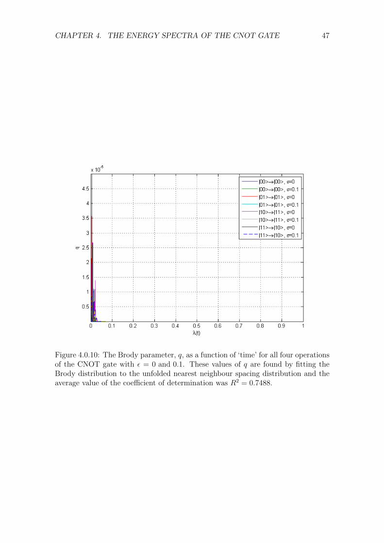
CHAPTER 4. THE ENERGY SPECTRA OF THE CNOT GATE 47
Figure 4.0.10: The Brody parameter, q, as a function of ‘time’ for all four operationsof the CNOT gate with ε = 0 and 0.1. These values of q are found by fitting theBrody distribution to the unfolded nearest neighbour spacing distribution and theaverage value of the coefficient of determination was R2 = 0.7488.

Chapter 5
The statistics of level occupation
for the CNOT gate
It is desirable to be able to run an adiabatic quantum computation process relatively
quickly, but at the same time we must try to ensure that the system remains in the
ground state so that solution can be accurately read out. Therefore, a compromise
between speed and adiabaticity must be reached. Knowledge of the relationship
between the computation rate or speed, λ = 1/T , and the success probability, i.e.
the probability of the system being found in the ground state at λ(t) = 0 given
that it was initially in the ground state with certainty, P (0(λ = 0)|0(λ = 1)),
will be very informative when trying to find this balance. The effects of noise
on this relationship are also an important consideration that should be taken into
account. In order to investigate this relationship, the energy spectra for an en-
semble of 50 random noise realisations for each of the 4 CNOT gate operations
were generated using the numerical techniques discussed in section 2.3 for solv-
ing the generalised Pechukas-Yukawa system ((2.1.34)). These spectra were then
analysed using the level occupation algorithm described in section 2.3 to find the
average success probabilities at a range of different computation speeds. It is im-
portant to note that this algorithm allows us to calculate the probability of the
system being found in the final ground state of the system’s total Hamiltonian (i.e.
H(λ = 0) = Hf + δh(λ = 0) = (HCNOT + Hinput) + δh(λ = 0)) as opposed to the
solution state (i.e. the ground state of Hf = HCNOT + Hinput). The distinction
between these two variables when noise comes into effect will be discussed later on
in this section.
The success probability as a function of computation speed for the |00〉 → |00〉operation at a range of noise amplitudes is shown in Fig. 5.0.1, including the case
of an ideal closed system (ε = 0). In general, we see a polynomial increase in
48

CHAPTER 5. THE STATISTICS OF LEVEL OCCUPATION FOR THE CNOTGATE49
success probability as the speed decreases, i.e. P ∝ T−γ. As the speed decreases
further we find that the success probability tends to unity, as expected from the
adiabatic theorem (1.2.14). These general trends and the polynomial dependence
are in agreement with the findings of [40] for random problem Hamiltonians drawn
from the GUE. A fit to the polynomial region of the ε = 0 curve yields a scaling
exponent of γ ≈ 4/3, whereas for ε > 0 we find the scaling exponents to all be
γ ≈ 1. The fact that this scaling remains constant as ε increases is heartening in
terms of the performance of AQC. When the noise source is switched on we see a
significant prefactor shift of the curves towards slower speeds as well as a decrease
in γ. This means that in some situations a speed 102 slower is required to achieve
the same chance of success. This is because the introduction of noise will split
any degeneracies into avoided crossings and it will also lead to fluctuations in the
level trajectories creating more avoided crossings. This increase in the number of
avoided crossings results in more opportunities for the system to be excited out
of the ground state and into higher levels, therefore a significantly slower speed is
required to achieve the same success probability as in the ideal case. This effect is
clearly not favourable, but some degree of noise is an inevitability in any physical
system and its effects must be considered.
An interesting feature to note in Fig. 5.0.1 is that, as ε increases we see a prefac-
tor shift in the curves back towards faster computation speeds. This can be seen as
being beneficial in the context of AQC as it means that the success probability at
a given computation speed increases linearly with noise amplitude.This occurs be-
cause stronger noise fluctuations will widen the energy gaps at avoided crossings, as
predicted by Fig. 4.0.7 where the average energy gaps generally increase with noise
amplitude, and therefore decrease the chance of excitation at that particular avoided
crossing. However, at |λ| ≈ 10−5 we see a change in the scaling and the curves of
increasing amplitude reverse in order. This can be explained by looking at whether
higher levels come into play in terms of the occupation, as shown in Fig. 5.0.2. For
small ε, we see a very sudden switch from P1 � P0 to P0 � P1 at |λ| ≈ 10−5 and no
occupation of the higher levels. This shows that the avoided crossing between x0(λ)
and x1(λ) is the limiting factor, meaning the success probability saturates quickly
and the gradient of the logarithmic plot stays constant. For larger ε, we have a more
complicated evolution of the level occupation as higher levels come into effect and
therefore the switch from P1 � P0 to P0 � P1 is not as sudden meaning the success
probability saturates more slowly and the gradient decreases. This slow down in
scaling is proportional to ε which leads to the reversal of the ordering of curves of
constant ε seen in Fig. 5.0.1.
The dependence of the success probability on the computation speed for the

CHAPTER 5. THE STATISTICS OF LEVEL OCCUPATION FOR THE CNOTGATE50
Figure 5.0.1: Plot of average success probability against computation speed for the|00〉 → |00〉 operation of the CNOT gate at various noise amplitudes.
|01〉 → |01〉 operation of the CNOT gate is shown in Fig. 5.0.5. For this operation,
we do not have a curve for an ideal system (ε = 0) to compare the effects of noise
against, as the success probability will be zero at all speeds when ε = 0, because of
degeneracy between the ground and first excited states. The same general trends
seen in Fig. 5.0.1 hold true in Fig. 5.0.3, in that the success probability increases
polynomially with computation time before saturating at one. In this case, we also
have constant scaling exponents of γ ≈ 1 and therefore an approximately inverse
linear relationship between success probability and computation speed. We can also
see that the prefactor shift of the curves is much greater than in Fig. 5.0.1. This
will be due to the fact that noise will have a much greater influence on the gap
widths at avoided crossings, as they are the result of noise-induced level splitting
in this case. The increase in success probability with noise amplitude remains for
all speeds and we do not see the reversal seen in Fig. 5.0.1. This is because the
noise-induced ground state gaps in the spectrum of the |01〉 → |01〉 operation are
generally narrower than those seen in the spectrum of the |00〉 → |00〉 operation
and therefore the occupation will still be able to spread into higher excited states
at relatively slow speeds. This means we do not see the sudden switch in behaviour
as ε increases that we have for the |00〉 → |00〉 operation.
Another feature in Fig. 5.0.3 is the fluctuation in the ε = 0.1 curve at |λ| ≈ 10−3.
This can again be explained by looking at the role that higher levels play in the level

CHAPTER 5. THE STATISTICS OF LEVEL OCCUPATION FOR THE CNOTGATE51
(a) ε = 0.025
(b) ε = 0.1
Figure 5.0.2: Plot of average occupation of the lowest 5 levels at λ(t) = 0 for the|00〉 → |00〉 operation at ε = 0.025 and 0.1. The occupation of all levels above n = 4is zero.

CHAPTER 5. THE STATISTICS OF LEVEL OCCUPATION FOR THE CNOTGATE52
Figure 5.0.3: Plot of average success probability against computation speed for the|01〉 → |01〉 operation of the CNOT gate at various noise amplitudes.
occupation statistics. Figure 5.0.4 shows that at |λ| ≈ 10−3 the occupation of the
first and second excited states both fall away quickly as the success probability
increases. This switch in occupations will lead to the fluctuation we see in Fig.
5.0.3.
The dependence of the success probability on the computation speed and noise
amplitude for the |10〉 → |11〉 and |11〉 → |10〉 operations of the CNOT gate are
shown in Fig. 5.0.5 and Fig. 5.0.6 respectively. They both show very similar trends
to the |01〉 → |01〉 case in Fig. 5.0.3 and in all three cases we find a constant scaling
exponent of γ ≈ 1. This is to be expected as they all have similar spectra, where
noise fluctuations and symmetry breaking create the sequences of avoided crossings
across which the occupation diffuses. There is a kink in the ε = 0.025 curve of Fig.
5.0.5; this can be explained by the same mechanism that causes the one seen in the
ε = 0.1 curve of Fig. 5.0.3. We can also see that the ε = 0.05 and ε = 0.075 curves
in Fig. 5.0.6 cross; this is readily explained by the mechanism that leads to the
crossing of curves of constant ε in the |00〉 → |00〉 case.
As we have seen, there are situations where an increase in noise amplitude will
increase the success probability of an AQC process, but it may not be wholly benefi-
cial, as it will also drive the final state of the system away from the desired solution

CHAPTER 5. THE STATISTICS OF LEVEL OCCUPATION FOR THE CNOTGATE53
Figure 5.0.4: Plot of average occupation of the lowest 5 levels at λ(t) = 0 for the|01〉 → |01〉 operation at ε = 0.1. The occupation of all levels above n = 4 is zero.
Figure 5.0.5: Plot of average success probability against computation speed for the|10〉 → |11〉 operation of the CNOT gate at various noise amplitudes.

CHAPTER 5. THE STATISTICS OF LEVEL OCCUPATION FOR THE CNOTGATE54
Figure 5.0.6: Plot of average success probability against computation speed for the|11〉 → |10〉 operation of the CNOT gate at various noise amplitudes.
state. This will affect the probability of the measurement of the final state yielding
the correct result. This is a different issue to the aforementioned success probability
in that, even if the system evolves at an infinitely slow rate, so that it will be in the
ground state at λ = 0 with certainty, if noise perturbations have driven |ψ(λ = 0)〉away from the ideal solution state the correct answer will not always be found upon
measurement. This is an important effect that must be accounted for when we are
studying the effect of noise in an AQC system.
To investigate this we introduce a measure of closeness between the ideal ground
state (i.e. when ε = 0) and the noise perturbed ground state (i.e. where ε > 0),
namely the fidelity of the final state;
F = |〈0ideal(λ = 0)|0noise(λ = 0)〉|2 . (5.0.1)
We calculate the fidelity by direct diagonalisation of; H0 = HCNOT +Hinput to find
|0ideal(λ = 0)〉 and, H0 + δh(0) to give |0noise(λ = 0)〉. This is then averaged over
an ensemble of noise realisations. Another way of taking this issue into account
would be to define success probability of an AQC in the presence of noise as P =
|〈0ideal|ψ(0)〉|2 instead of simply the ground state occupation at λ = 0, as in [7]. This
is not possible with our current approach as we do not have specific knowledge of the
state vector, but we can look at the relationship between these two important factors.

CHAPTER 5. THE STATISTICS OF LEVEL OCCUPATION FOR THE CNOTGATE55
Figure 5.0.7: Plot showing the average fidelity of the final state and average successprobability as functions of noise amplitude for the |00〉 → |00〉 operation.
In other recent work [50] (manuscript included in appendix C), we investigated the
time average of this quantity for a large set of random problem instances and found
that it generally increased smoothly with the final ground state occupation, although
these results did not take into account the effects of noise.
The fidelity of the final state and the success probability of the |00〉 → |00〉operation are shown as functions of noise amplitude in Fig. 5.0.7. As ε increases,
|0noise(λ = 0)〉 is driven further away from |0ideal(λ = 0)〉 and the fidelity decreases
linearly. We can also clearly see that success probabilities that are comparable to
the fidelity lie at speeds above the reversal in Fig. 5.0.1, as they too decrease linearly
with ε.
Figure 5.0.8 shows the relationship between the fidelity, success probability and
noise amplitude for the |01〉 → |01〉 operation of the CNOT gate. In this case, we can
see that the success probability at a given speed increases linearly with ε, whereas
the fidelity of the final state decreases linearly, so we have a trade-off between these
two effects. Therefore, at the intersection of the lines we have an optimal noise
amplitude that maximises both the fidelity and the success probability.
The fidelity and the success probability of the |10〉 → |11〉 and |11〉 → |10〉operations behave in a similar fashion to the |01〉 → |01〉 operation, as seen in
Fig. 5.0.9 and Fig. 5.0.10 respectively. This is because their spectra show similar
trends and properties and therefore they show similar behaviour with respect to
level occupation.

CHAPTER 5. THE STATISTICS OF LEVEL OCCUPATION FOR THE CNOTGATE56
Figure 5.0.8: Plot showing the average fidelity of the final state and average successprobability as functions of noise amplitude for the |01〉 → |01〉 operation.
Figure 5.0.9: Plot showing the average fidelity of the final state and average successprobability as functions of noise amplitude for the |10〉 → |11〉 operation.

CHAPTER 5. THE STATISTICS OF LEVEL OCCUPATION FOR THE CNOTGATE57
Figure 5.0.10: Plot showing the average fidelity of the final state and average successprobability as functions of noise amplitude for the |11〉 → |10〉 operation.
Certain types of algorithms, particularly optimisation problems like the traveling
salesman (TSP), are suited to a less stringent version of AQC known as approximate
adiabatic quantum computation (AAQC). In AAQC we require only that the system
remains close to, but not necessarily in, its ground state, as for optimisation problems
like the TSP this will still yield a near-optimal result. This relaxation of requirements
will allow the computation process to be run at significantly faster speeds [51]. The
fact that we do not see a significant deviation away from the ground state in Fig.
5.0.2 and Fig. 5.0.4, even when the success probability ∼ 0, for a generic adiabatic
algorithm is a promising result for AAQC.
To summarise, we have found that the success probability of the CNOT gate
algorithm scaled polynomially as a function of computation speed. This scaling
was shown to be independent of the amplitude of the noise, which is a promising
point to note in terms of the performance of a realistic AQC process. Somewhat
counterintuitively, we have also seen that in some situations, noise increases the
success probability at a given speed, particularly when there are degeneracies in the
energy spectra. However, it was noted that this increase comes at the expense of
the fidelity of the final state, but an optimal compromise between the two factors
exists. We have shown that an insight into spectral properties and statistics can be
useful when trying to explain level occupation phenomena.

Chapter 6
The CNOT gate with an artificial
noise source
In the previous chapter, 5, we saw that the intrinsic noise in a physical system can
improve the performance of an AQC in some situations. We now look at this from
a different viewpoint and envisage a system with a negligibly low level of intrinsic
noise and try to enhance its performance by adding a specifically tailored artificial
noise source. This can be seen as a stochastic search for an alternative, and possibly
more efficient, path between the initial and final Hamiltonians than simple linear
interpolation.
To achieve this we require a perturbation term with a time-dependent amplitude,
which is large enough to widen the energy gaps at avoided crossings throughout the
majority of the computation process but then tends to zeros as λ(t)→ 0. We need
to be particularly careful in the region where λ(t) & 0 where the energy levels are
densely packed and the majority of excitation occurs, as we would like to retain
positive effects of noise, while at the same time minimising the negative effect on
the fidelity of the final state. As an example of this scheme, we retain the same
noise model used throughout this work except that we introduce a time-dependent
amplitude of the form
ε(λ) = ε0 tanh(αλ), (6.0.1)
where α is a constant determining the rate of decay as λ(t) & 0.
The dependence of the success probability on the computation speed for the
|00〉 → |00〉 operation with an artificial noise source is shown Fig. 6.0.1. The
constant α was varied in order to find the type of behaviour we were looking for. It
was found that a value of α = 10 yielded a significant prefactor improvement, up to
102 in some cases, over the results for a noise source with a constant amplitude. This
improvement occurs because we have strong noise fluctuations that drive the levels
58

CHAPTER 6. THE CNOT GATE WITH AN ARTIFICIAL NOISE SOURCE 59
and their trajectories away from each other in the early part of the computation
process where there is little chance of excitation. Then as the system moves into the
critical final part of the evolution where the levels are densely packed, the strength
of the artificial perturbations are reduced to zero to avoid creating any more avoided
crossings and therefore reducing the chance of excitation.
The effects of an artificial noise source on the success probabilities of the other
operations of the CNOT gate are shown in Fig. 6.0.2, Fig. 6.0.3 and Fig. 6.0.4. A
value of α = 10 was again used and the results are compared to those for a noise
source with a constant amplitude. We again see a significant prefactor improvement.
Particularly for the |11〉 → |10〉 operation, where there is a remarkable improvement
of over 5 orders of magnitude. These improvements will occur for the same reasons
described for the |00〉 → |00〉 operation.
Another advantage of this scheme is the fact that the artificial noise will not affect
the fidelity of the final state. As we can see from (6.0.1), ε(0) = 0 and therefore the
final ground state will coincide with the desired solution state yielding F = 1.
In this chapter we have shown that it is possible to drastically improve the
performance of an AQC by the addition of a specifically engineered artificial noise
source. This would allow the same computation to be run at speeds of up to 105
times faster while still maintaining the same success probability. This scheme can
also be realised in such a way that it will have no adverse effect on the fidelity of
the final ground state. Although these results are heartening, it is important to
note that they are based on the assumption that we have a physical system with a
negligibly small amount of intrinsic noise, which in terms of current technologies is
fairly unrealistic. Despite this, these results do lend support to the idea that simple
linear interpolation between initial and final Hamiltonians is not always the most
efficient evolution path. This idea is an important consideration which should be
taken account of when discussing the performance of AQC, e.g. as in [20].

CHAPTER 6. THE CNOT GATE WITH AN ARTIFICIAL NOISE SOURCE 60
Figure 6.0.1: Plot of average success probability against computation speed for the|00〉 → |00〉 operation of the CNOT gate with an artificial noise source at a range ofvalues for ε0 and α = 10. For comparative purposes, the results for a noise sourcewith a constant amplitude of ε = 0.025 are also shown.
Figure 6.0.2: Plot of average success probability against computation speed for the|01〉 → |01〉 operation of the CNOT gate with an artificial noise source at a range ofvalues for ε0 and α = 10. For comparative purposes, the results for a noise sourcewith a constant amplitude of ε = 0.1 are also shown.

CHAPTER 6. THE CNOT GATE WITH AN ARTIFICIAL NOISE SOURCE 61
Figure 6.0.3: Plot of average success probability against computation speed for the|10〉 → |11〉 operation of the CNOT gate with an artificial noise source at a range ofvalues for ε0 and α = 10. For comparative purposes, the results for a noise sourcewith a constant amplitude of ε = 0.1 are also shown.
Figure 6.0.4: Plot of average success probability against computation speed for the|11〉 → |10〉 operation of the CNOT gate with an artificial noise source at a range ofvalues for ε0 and α = 10. For comparative purposes, the results for a noise sourcewith a constant amplitude of ε = 0.1 are also shown.

Chapter 7
The extended Pechukas-Yukawa
system
In the results presented in chapters 5 and 6, the level occupation probabilities are
estimated by analysis of the structure of the energy spectrum. However, as noted
in chapter 5 it would be beneficial to have a complete description of the state of a
quantum system, as opposed to just the occupations. In light of this we now derive
a novel extended version of the Pechukas-Yukawa framework that allows a complete
description of the quantum state.
If we start with the operator equation of motion derived during the derivation
of the generalised Pechukas-Yukawa model (2.1.9),
d
dλAnm = i
∑k
(HnkAkm − AnkHkm) + 〈n| ∂A∂λ|m〉 , (7.0.1)
and insert the density operator, ρ = |ψ〉 〈ψ|, for A we have
d
dλρnm = i
∑k
(Hnkρkm − ρnkHkm) + 〈n| ∂ρ∂λ|m〉 . (7.0.2)
The term outside the sum, the partial time derivative of ρ is described by the Von
Neumann equation, ∂ρ/∂λ = −i [H, ρ] and we also know that
∂ρ
∂λ=∂ρ
∂t
∂t
∂λ, (7.0.3)
therefore we have
〈n| ∂ρ∂λ|m〉 =
∂t
∂λ〈n| − i [H, ρ] |m〉 = −i ∂t
∂λ(〈n|Hρ |m〉 − 〈n| ρH |m〉) , (7.0.4)
where H is the Hamiltonian not the operator H. We can define the density operator
62

CHAPTER 7. THE EXTENDED PECHUKAS-YUKAWA SYSTEM 63
as an element by element sum
ρ =∑a,b
ρab |a〉 〈b| , (7.0.5)
and insert it into (7.0.4) to give
〈n| ∂ρ∂λ|m〉 = −i ∂t
∂λ
∑a,b
ρab (〈n|H |a〉 〈b|m〉 − 〈n|a〉 〈b|H |m〉) . (7.0.6)
Using the eigenvalue equation H |n〉 = xn |n〉 we have
〈n| ∂ρ∂λ|m〉 = −i ∂t
∂λ
∑a,b
ρab (xa 〈n|a〉 〈b|m〉 − xm 〈n|a〉 〈b|m〉) , (7.0.7)
due to orthgonality, 〈n|m〉 = δnm, the only non-zero contribution to this sum will
come when n = a and m = b, which gives
〈n| ∂ρ∂λ|m〉 = −i ∂t
∂λρnm (xn − xm) . (7.0.8)
Therefore we have
d
dλρnm = i
∑k
(Hnkρkm − ρnkHkm)− iρnm (xn − xm) , (7.0.9)
where Hab is defined by the following identity found during the derivation of the
standard Pechukas-Yukawa model [46]
Hab =Vab
i (xa − xb), (7.0.10)
which is analogous to equation (2.1.13) for the generalised Pechukas-Yukawa system.
If we first consider the diagonal elements of the density matrix, i.e. where n = m
in (7.0.9), we have
d
dλρnn = i
∑k 6=n
(Hnkρkn − ρnkHkn)− 0. (7.0.11)
Then, using (7.0.10) and the Yukawa dynamical variable, lnm = (xn − xm)Vnm, we

CHAPTER 7. THE EXTENDED PECHUKAS-YUKAWA SYSTEM 64
have
d
dλρnn =
∑k 6=n
(Vnkρkn
(xn − xk)− ρnkVkn
(xk − xn)
), (7.0.12)
=∑k 6=n
(Vnkρkn + ρnkVkn
(xn − xk)
), (7.0.13)
=∑k 6=n
(lnkρkn + ρnklkn
(xn − xk)3
). (7.0.14)
As both l and ρ are Hermitian we can say that
d
dλρnn =
∑k 6=n
(2 |lnkρkn|
(xn − xk)3
)= pn, (7.0.15)
where pn are the occupations or populations of a given eigenlevel n.
If we now consider the case of the off-diagonal elements of ρ, i.e. where n 6= m
in (7.0.9), we have
d
dλρnm = i
∑k 6=n,m
(Hnkρkm − ρnkHkm)− i ∂t∂λρnm (xn − xm) . (7.0.16)
Using (7.0.10) and lnm = (xn − xm)Vnm we have
d
dλρnm =
∑k 6=n,m
(Vnkρkm
(xn − xk)− ρnkVkm
(xk − xm)
)− i ∂t
∂λρnm (xn − xm) , (7.0.17)
=∑k 6=n,m
(lnkρkm
(xn − xk)2+
ρnklkm(xm − xk)2
)− i∂λ
∂tρnm (xn − xm) . (7.0.18)
These terms, ρnm, describe the inter-level coherences, i.e. the matrix element be-
tween eigenstates |n〉 and |m〉.We now have a pair of equations,
pn =∑k 6=n
(2 |lnkρkn|
(xn − xk)3
)ρnm =
∑k 6=n,m
(lnkρkm
(xn − xk)2+
ρnklkm(xm − xk)2
)− i∂λ
∂tρnm (xn − xm) , (7.0.19)
that when used in conjunction with the standard Pechukas-Yukawa equations, (1.3.2),
form a closed system of classical equations of motion that fully capture both the
dynamics of the eigenvalues and the state of the system. They therefore completely
describe the dynamics of the quantum system and this is done without making

CHAPTER 7. THE EXTENDED PECHUKAS-YUKAWA SYSTEM 65
any simplifications or assumptions. It may also be possible to generalise (7.0.19)
to the dissipative case by starting with a master equation instead of the Von Neu-
mann equation. These equations could be a useful result as they allow the use of
techniques and approaches from classical physics, that do not neccesarily have a
quantum analogue, to be readily applied to quantum mechanical systems.

Chapter 8
Conclusions
In this work we have derived a generalised stochastic form of the Pechukas-Yukawa
model of eigenvalue dynamics. This allowed us to take into account the effects of a
simple, yet generic, coloured noise source on the system’s evolution. We used this
approach to study an example of a prototypical adiabatic quantum algorithm which
involves 4 qubits; the GSQC form of the CNOT gate.
We have studied the energy spectra and their spectral properties and seen how
noise affects these. In particular, we showed that the presence of noise will break any
degeneracies in the spectrum that might obstruct the computation process without
significantly disturbing the regularity of the eigenvalue dynamics. We then studied
the effects of noise on the statistics of level occupation by analysing the sequences
of avoided crossings in the spectra that can lead to excitation out of the ground
state. In general, we found that the success probability scales polynomially with the
computation speed and noise introduces a shift of prefactor into this relationship. We
then investigated a theoretical situation where we have the opportunity to greatly
improve the success rate of the computation by the addition of a specifically tailored
artificial noise source. Finally, we formulated an extended version of the Pechukas-
Yukawa model that provides a complete description of the dynamics of the quantum
state, as well as the eigenvalues. This maintains the key benefit of being an exact
map to a classical system of equations of motion. We have demonstrated that an
eigenvalue dynamics approach can offer an insightful alternative to the Schrodinger
picture, as we have shown that detailed knowledge of a quantum system’s energy
spectrum and its properties can help explain the system’s behaviour. From these
results there are two main conclusions we can draw.
The first is on the relative robustness of an AQC process against the effects
of noise. In chapter 4, we showed that despite the addition of a relatively strong
irregularity into our system, i.e. noise, the overall eigenvalue dynamics remain
regular. This is a promising result, as it means that small random fluctuations in
66

CHAPTER 8. CONCLUSIONS 67
the Hamiltonian should not lead to radical changes in the dynamics of the system
and therefore we can expect the results of the computation to be reasonably close
to the desired results. This demonstrates the stability of the AQC process in the
presence of noise. We have also shown that the polynomial dependence of the success
probability on the computation speed is independent of the noise amplitude. This
result demonstrates the robustness of the performance of AQC in the presence of
noise. In fact we have shown that in some situations, noise can provide a linear
increase in the success probability at a given speed. Although this improvement
comes at the cost of the fidelity of the final state, there exists a noise amplitude that
offers an optimal compromise. The idea of noise providing an improvement in the
performance of a device is counter-intuitive, however there is some precedence for
this in the context of AQC, [7, 12].
The second main conclusion we can draw from this work is with regards to the
choice of initial conditions in AQC. We have analysed situations where symmetries
in the Hamiltonian lead to degeneracies in the spectrum, including some where de-
generacies between the ground and first excited state would lead to failure of the
computation process. We have shown that in realistic systems, where the perturba-
tive effects of noise are taken into account, all of these symmetries and degeneracies
will be broken naturally. This means there will always be a finite success probability
in practical AQC systems and therefore we can say that the conventional stipula-
tion that the initial and final Hamiltonians do not commute is unnecessary. In
fact, it is when the initial and final Hamiltonians commute that we see the greatest
noise-enhancement of the performance. This is an important result as it removes a
restriction on the choice of initial Hamiltonian that may prove practically impossible
to realise for universal AQC.
These results have been published in [52] and a copy of the manuscript is included
in appendix B.
8.1 Suggestions for further work
We believe there are a number of different directions in which this work could be
taken that may provide some fruitful and insightful results.
The most straightforward extension of this work would be to look at the effects
of noise on different types of adiabatic quantum algorithms. Determining how the
computation time of a given algorithm scales with input size (no. of qubits), effec-
tively the algorithmic efficiency, is a crucial step in evaluating its performance and
practicality. Therefore, it would be interesting to investigate how noise affects this
scaling in an algorithm with a variable input size. As mentioned in section 1.2.3.2,
CHAPTER 8. CONCLUSIONS 68
an example of an NP-complete algorithm that is often studied is the boolean satis-
fiability (SAT) problem and that prior attempts to determine whether AQC can be
used to efficiently solve this problem have been mixed. It is currently believed that
relatively easy SAT problem instances, which have a high degree of structure to
them, can be solved efficiently using AQC (e.g. as in [6]), but there is some debate
as to whether this holds for hard instances of the SAT problem (e.g. as reviewed in
[17]). So far, to our knowledge, the effects of noise on the efficiency on the different
types of SAT problem instances have not been directly explored. It could be the
case that the addition of noise may affect the structure in the Hamiltonian that
determines the efficiency of that particular problem instance.
When discussing the efficiency of any computational algorithm it is necessary to
consider its performance in the limit of large system sizes. Unfortunately, the num-
ber of dimensions of the Hilbert space required to describe the state of a quantum
information processing system in the Schrodinger picture grows exponentially with
the number of qubits; this means it is very difficult to try to evaluate the behaviour
of quantum algorithms in the limit of large input sizes. The method of numeri-
cally solving the Pechukas-Yukawa equations used in the simulations in section 2.3
suffers from the same scalability problems as directly solving the Schrodinger equa-
tion (i.e. the dimension of the phase space needed to describe the state of the
eigenvalue gas grows exponentially with the input size). However, the eigenvalue
gas described by the Pechukas-Yukawa equations is a classical system unlike the
Schrodinger equation, which means that techniques for dealing with large systems
from classical statistical physics are applicable. The use of Klimontovich’s kinetic ap-
proach (described in [53]) is proposed in [40]; where the Pechukas-Yukawa system of
equation are rewritten as a BBGKY (Bogoliubov-Born-Green-Kirkwood-Yvon) type
chain of equations for the macroscopic (or average) distribution functions f1 = 〈F1〉,f2 = 〈F2〉, g2 = 〈G2〉,..., where
F1(x, v, t) =∑
1≤i≤N
δ(x− xi(t))δ(v − vi(t)), (8.1.1)
F2(x(m), v(m), x(n), v(n), l(mn), t) =
∑1≤i<j≤N
δ(x(m) − xi(t))δ(v(m) − vi(t))
δ(x(n) − xj(t))δ(v(n) − vj(t))δ(l(mn) − lij(t)) and (8.1.2)
G2(l, t) =∑
1≤i<j≤N
δ(l − lij(t)) (8.1.3)
are the microscopic distribution functions. Then using the standard method of

CHAPTER 8. CONCLUSIONS 69
truncating the BBGKY chain an equation of motion for f1 can be derived. Recent
results have suggested that the bulk of the eigenspectrum of an adiabatic quantum
computer may have little effect on the overall dynamics of the system (see [18]) and
that it is the eigenlevels on the edges of the spectrum that are important. This means
that large systems could be investigated by directly simulating a few eigenvalues on
the edges of the spectrum using the Pechukas-Yukawa equations and then taking
account of the long-range influence of the bulk of the spectrum statistically using
the kinetic equations.
In section 6, we explored the idea of making use of a controllable artificial noise
source to try to improve the performance of an AQC operation. A more obvious
choice of variable to control is the computation speed,∣∣∣λ∣∣∣, as we know that decreas-
ing this will directly increase the success probability. However, at the same time
we would clearly like to be able to run practical computations as fast as possible.
In light of this, we envision an AQC system whose speed is dynamically controlled.
This would allow the computation to be run relatively quickly for the majority of the
evolution but then the speed could be reduced at the critical points where excitation
out of the ground state may occur (e.g. near avoided crossings), therefore allowing
a high rate of success to be achieved at relatively short total computation times. To
realise this we would require a type of continuous, weak measurement that could
detect when the system is approaching one of these critical points. In [29], non-
destructive continuous measurement of the ground state curvature of a flux qubit
was demonstrated experimentally using the impedance measurement technique with
a high quality tank circuit. The ground state curvature would be a suitable control
variable, as we expect it to increase at avoided crossings. This could be readily
modeled using the Pechukas-Yukawa formalism as the ground state curvature will
be proportional to |l01(λ)|. To properly analyse the effects of this control system we
will need to be able to calculate the probabilities of level occupation in the contin-
uum within the Pechukas-Yukawa formalism as opposed to the discrete algorithm
detailed in section 2.3; the derivation of a novel extension of the Pechukas-Yukawa
equation that would allow this is detailed in chapter 7. The computation speed
within these equations can be defined in a such way that it is dynamically related to
|l01(λ)|. We therefore have all the necessary components to model an AQC system
where the computation speed is dynamically controlled via a feedback loop that
performs continuous measurement of the ground state curvature and then analyse
the effects of this control system on the success probability. Feedback control sys-
tems are widely used in many engineering applications and their theory is a well
understood branch of control systems theory [54]; we would be able to draw on this
knowledge when designing a feedback controller for an AQC system.
CHAPTER 8. CONCLUSIONS 70
In other recent results, [50] and appendix C, we have explicitly investigated
the relationship between the success probability and the minimum ground state
energy gap in AQC. We show that there exists a rich structure in the distribution
of these two figures of merit. The structure of distinct sharp edges and densely
populated bands seen in the distribution is reminiscent of the projection of a higher
dimensional surface on to a plane. One possible explanation of this could be that the
the structure we see is the shadow of the system’s surface of adiabatic invariance. An
adiabatic invariant is a constant of motion of a dynamical system that is preserved
in the adiabatic limit, because of this they can be considered to be an asymptotic
statement. They are well known in classical mechanics [55]. Knowledge about the
adiabatic invariants of an AQC could prove to be very insightful, as it would improve
our understanding of the relationship between the system’s control parameters and
measures of its performance. This could have a major impact on algorithm and
system design in the field of AQC. The Pechukas-Yukawa formalism would be a
particularly useful tool in this endeavour. By taking advantage of the fact that
it reduces the dynamics of a quantum system to a system of classical equations of
motion; approaches and techniques from the study of adiabatic invariants in classical
mechanics could then be applied. For instance, the action of a classical system is
always an adiabatic invariant. It would be possible to write a Hamiltonian and
Lagrangian for the Pechukas gas and therefore formulate the action integral for a
generic quantum system.

Appendix A
Program listings
A.1 Simulation programs
The following MATLAB script and dependent functions will generate the energy
spectra for a large set of noise realisations applied to a specific operation of the
adiabatic CNOT gate;
1 %∗∗∗∗∗∗∗∗∗∗∗∗∗∗∗∗∗∗∗∗∗∗∗∗∗∗∗∗∗∗∗∗∗∗∗∗∗∗∗∗∗∗∗∗∗∗∗∗∗∗∗∗∗∗∗∗∗∗∗∗∗∗∗∗∗∗∗∗∗∗∗∗∗∗∗∗∗∗2 %CNOT gate noise ins tance generator
3 %∗∗∗∗∗∗∗∗∗∗∗∗∗∗∗∗∗∗∗∗∗∗∗∗∗∗∗∗∗∗∗∗∗∗∗∗∗∗∗∗∗∗∗∗∗∗∗∗∗∗∗∗∗∗∗∗∗∗∗∗∗∗∗∗∗∗∗∗∗∗∗∗∗∗∗∗∗∗4 %This s c r i p t genera te s a s e t number o f random noise in s tance s and app l i e s them
5 %to the e vo l u t i on o f the ada i a ba t i c CNOT gate us ing the g ene ra l i s e d
6 %Pechukas−Yukawa model
7 %
8 %Dependencies : co l oured no i s e .m, g e n e r a l i s e d p e r t u r b i n i t i a l .m,
9 %genera l i sed pechukas yukawa sys tem .m
10 %∗∗∗∗∗∗∗∗∗∗∗∗∗∗∗∗∗∗∗∗∗∗∗∗∗∗∗∗∗∗∗∗∗∗∗∗∗∗∗∗∗∗∗∗∗∗∗∗∗∗∗∗∗∗∗∗∗∗∗∗∗∗∗∗∗∗∗∗∗∗∗∗∗∗∗∗∗∗11
12 clc
13 clear
14
15 global l e v e l s nu vec tau lambda step lambda length dh vec ;
16
17 %Seed random number generator
18 RandStream . setDefau l tStream (RandStream( ’ mt19937ar ’ , ’ seed ’ ,100) ) ;
19
20 %Define cons tant s and parameters
21 l e v e l s =16; %no . o f energy l e v e l s in the system
22 momenta=l e v e l s ˆ2 ; %no . o f l mn needed to de s c r i b e the i n t e r a c t i o n s in the ←↩Pechukas gas
23 CNOT op=1; %CNOT operat ion |00> −> |00>24 ep s i l o n =−0.1; %energy s c a l e
25 z=10; %bia s
26 Eb=[−8:−1 ,1:8] ; %Eigenspectrum of H b ( i n i t i a l Hamiltonian )
27 d=−0.1;
28 dd=[d , d , d , d , d , 0 , 0 , 0 , d , 0 , 0 , 0 , d , 0 , 0 , 0 ] ;
29 %apply smal l random per tu r ba t i on s to eigenspectrum of H b
30 for k=1: l e v e l s
31 Eb(k )=Eb(k ) +1.5∗(dd (k ) /d) ;32 end
71

APPENDIX A. PROGRAM LISTINGS 72
33 tau =0.1; %noise c o r r e l a t i on time
34 n r epea t s =50; %no . o f r epea t s at each g iven noise ampl i tude
35 amp range = [ 0 . 0 2 5 , 0 . 0 5 , 0 . 0 7 5 , 0 . 1 ] ; %noise ampl i tudes
36 lambda step =0.005; %noise time s t ep
37 l ambda f in e s t ep =0.00001; %f in e s t ep to use when i n t e g r a t i n g f o r lambda ( t ) near 0
38 lambda=1:− lambda step : 0 ; %noise time i n t e r v a l
39 lambda f ine=[1:− lambda step :0 .1 ,0 .1 − l ambda f in e s t ep :− l ambda f in e s t ep : 0 ] ; %←↩Pechukas i n t e g r a t i on time i n t e r v a l
40 lambda length=length ( lambda ) ;
41 s a v e d i r=’C:\Documents and Se t t i n g s \phrdw2\My Documents\CNOT data \00 to00 ’ ; %root ←↩d i r e c t o r y
42
43 %Set up CNOT Hamiltonian
44 c 00=zeros (5 ) ;
45 c 00 (1 , 2 ) =1;
46 c 00=qo ( c 00 ) ;
47 c 01=zeros (5 ) ;
48 c 01 (1 , 3 ) =1;
49 c 01=qo ( c 01 ) ;
50 c 10=zeros (5 ) ;
51 c 10 (1 , 4 ) =1;
52 c 10=qo ( c 10 ) ;
53 c 11=zeros (5 ) ;
54 c 11 (1 , 5 ) =1;
55 c 11=qo ( c 11 ) ;
56 I=i d en t i t y (5 ) ;
57 c 000=tenso r ( c 00 , I ) ;
58 c 100=tenso r ( I , c 00 ) ;
59 c 001=tenso r ( c 01 , I ) ;
60 c 101=tenso r ( I , c 01 ) ;
61 c 010=tenso r ( c 10 , I ) ;
62 c 110=tenso r ( I , c 10 ) ;
63 c 011=tenso r ( c 11 , I ) ;
64 c 111=tenso r ( I , c 11 ) ;
65 H cnot=c 010 ’ ∗ ( c 110 ’∗ c 110+c 111 ’∗ c 111 ) ∗ c 010 − c 010 ’ ∗ ( c 110 ’∗ c 100+c 111 ’∗ ←↩c 101 ) ∗ c 000 − c 000 ’ ∗ ( c 100 ’∗ c 110+c 101 ’∗ c 111 ) ∗ c 010 + c 000 ’ ∗ ( c 100 ’∗ ←↩c 100+c 101 ’∗ c 101 ) ∗ c 000 . . .
66 +c 011 ’ ∗ ( c 110 ’∗ c 110+c 111 ’∗ c 111 ) ∗ c 011 − c 011 ’ ∗ ( c 110 ’∗ c 101+c 111 ’∗ c 100 ←↩) ∗ c 001 − c 001 ’ ∗ ( c 101 ’∗ c 110+c 100 ’∗ c 111 ) ∗ c 011+c 001 ’ ∗ ( c 101 ’∗ c 101+←↩c 100 ’∗ c 100 ) ∗ c 001 . . .
67 +(c 000 ’∗ c 000+c 001 ’∗ c 001 ) ∗( c 110 ’∗ c 110+c 111 ’∗ c 111 )+(c 010 ’∗ c 010+c 011 ←↩’∗ c 011 ) ∗( c 100 ’∗ c 100+c 101 ’∗ c 101 ) ;
68 i f CNOT op==1
69 de l ta H cnot=qo ( ep s i l o n ∗( c 000 ’∗ c 000+c 100 ’∗ c 100 ) ) ;
70 e l s e i f CNOT op==2
71 de l ta H cnot=qo ( ep s i l o n ∗( c 000 ’∗ c 000+c 101 ’∗ c 101 ) ) ;
72 e l s e i f CNOT op==3
73 de l ta H cnot=qo ( ep s i l o n ∗( c 001 ’∗ c 001+c 100 ’∗ c 100 ) ) ;
74 e l s e i f CNOT op==4
75 de l ta H cnot=qo ( ep s i l o n ∗( c 001 ’∗ c 001+c 101 ’∗ c 101 ) ) ;
76 end
77 H=H cnot+de l ta H cnot ;
78 H trunc=truncate (H, { 2 : 5 , 2 : 5 } ) ;
79
80 %∗∗∗∗∗∗∗∗∗∗∗∗∗∗∗∗∗∗∗∗∗∗∗∗∗∗∗∗∗∗∗∗∗∗∗∗∗∗∗∗∗∗∗∗∗∗∗∗∗∗∗∗∗∗∗∗∗∗∗∗∗∗∗∗∗∗∗∗∗∗∗∗∗∗∗∗81 for a=1: length ( amp range )
82 amp str ing=num2str( amp range ( a ) ) ;

APPENDIX A. PROGRAM LISTINGS 73
83 cu r r e n t d i r=s t r c a t ( save d i r , ’ \amp pt ’ , amp str ing ( 3 :end) ) ; %save d i r e c t o r y f o r ←↩current noise ampl i tude
84
85 amp=amp range ( a )
86 for n=1: n r epea t s
87
88 %Generate a s e t o f no ise matr ices and t h e i r d e r i v a t i v e s
89 h i n i t=amp.∗ wigner ( l e v e l s , 1 ) ;
90 h i n i t v e c=reshape ( h i n i t , l e v e l s ˆ2 ,1) ;
91 nu vec=zeros ( length ( lambda ) , l e v e l s ˆ2) ;
92 for k=1: length ( lambda )
93 nu=amp.∗ wigner ( l e v e l s , 1 ) ;
94 nu vec (k , : )=reshape (nu , 1 , l e v e l s ˆ2) ;
95 end
96
97 h vec=zeros ( length ( lambda ) , l e v e l s ˆ2) ;
98 [ lambda , h vec ]=ode23 ( @co loured no i se , lambda , h i n i t v e c ) ;
99
100 dh vec=zeros ( length ( lambda ) , l e v e l s ˆ2) ;
101 for k=1: length ( lambda )
102 dh vec (k , : )=−tau∗h vec (k , : )+nu vec ( ( length ( lambda )−round( lambda (k ) / ←↩lambda step ) ) , : ) ;
103 end
104
105 %Solve g ene ra l i s e d Pechukas equa t ions to generate the energy spectrum
106 %for t h i s noise ins tance
107 x v l i n i t i a l=g e n e r a l i s e d p e r t u r b i n i t i a l ( f u l l ( H trunc ( : , : ) ) , z ,Eb , h i n i t ) ←↩;
108 [ lambda f ine , x v l ]=ode113 ( @general i sed pechukas yukawa system , ←↩lambda f ine , x v l i n i t i a l ) ;
109
110 %Save the data f o r t h i s no ise ins tance
111 f i l e name=s t r c a t ( cu r r en t d i r , ’ \ run ’ ,num2str(n) , ’ . mat ’ ) ;
112 save ( f i l e name , ’n ’ , ’amp ’ , ’ x v l ’ , ’ h vec ’ , ’ dh vec ’ )
113
114 disp (n)
115 end
116 end
1 function dh=co l ou r ed no i s e ( lambda , h)
2 %∗∗∗∗∗∗∗∗∗∗∗∗∗∗∗∗∗∗∗∗∗∗∗∗∗∗∗∗∗∗∗∗∗∗∗∗∗∗∗∗∗∗∗∗∗∗∗∗∗∗∗∗∗∗∗∗∗∗∗∗∗∗∗∗∗∗∗∗∗∗∗∗∗∗∗∗∗∗3 %Coloured noise d i f f e r e n t i a l equat ion
4 %∗∗∗∗∗∗∗∗∗∗∗∗∗∗∗∗∗∗∗∗∗∗∗∗∗∗∗∗∗∗∗∗∗∗∗∗∗∗∗∗∗∗∗∗∗∗∗∗∗∗∗∗∗∗∗∗∗∗∗∗∗∗∗∗∗∗∗∗∗∗∗∗∗∗∗∗∗∗5 %This func t i on re turns the vec to r form of the d e r i v a t i v e o f the random matrix
6 %noise term \ de l t ah (\ lambda ) in the g ene ra l i s e d Pechukas−Yukawa model .
7 %It ’ s e vo l u t i on i s de s c r i b ed the Ornstein−Uhlenbeck process .
8 %I t re turns the d e r i v a t i v e in a form s u i t a b l e f o r the ODE so l v e r s u i t e .
9 %∗∗∗∗∗∗∗∗∗∗∗∗∗∗∗∗∗∗∗∗∗∗∗∗∗∗∗∗∗∗∗∗∗∗∗∗∗∗∗∗∗∗∗∗∗∗∗∗∗∗∗∗∗∗∗∗∗∗∗∗∗∗∗∗∗∗∗∗∗∗∗∗∗∗∗∗∗∗10
11 global l e v e l s nu vec tau lambda step lambda length dh vec ;
12 dh=zeros ( l e v e l s ˆ2 ,1) ;
13 nu=zeros (1 , length ( l e v e l s ˆ2) ) ;
14 %f ind va lue s o f whi te noise term \nu(\ lambda ) at \ lambda us ing l i n e a r ←↩i n t e r p o l a t i o n
15 for k=1: l e v e l s ˆ2
16 nu(k )=interp1 ( [1 :− lambda step : 0 ] , nu vec ( : , k ) , lambda , ’ n ea r e s t ’ ) ;
17 end
18 %Ornstein−Uhlenbeck equat ion
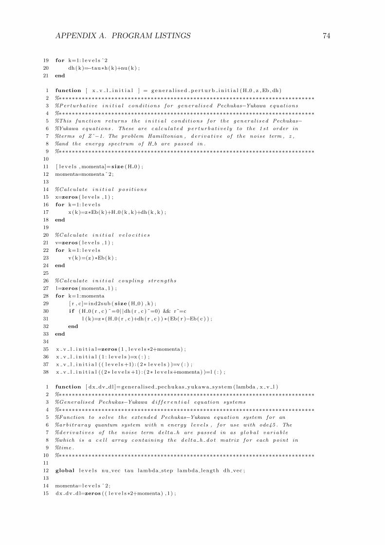
APPENDIX A. PROGRAM LISTINGS 74
19 for k=1: l e v e l s ˆ2
20 dh(k )=−tau∗h(k )+nu(k ) ;
21 end
1 function [ x v l i n i t i a l ] = g e n e r a l i s e d p e r t u r b i n i t i a l (H 0 , z ,Eb , dh)
2 %∗∗∗∗∗∗∗∗∗∗∗∗∗∗∗∗∗∗∗∗∗∗∗∗∗∗∗∗∗∗∗∗∗∗∗∗∗∗∗∗∗∗∗∗∗∗∗∗∗∗∗∗∗∗∗∗∗∗∗∗∗∗∗∗∗∗∗∗∗∗∗∗∗∗∗∗∗∗3 %Per turba t i v e i n i t i a l cond i t i ons f o r g ene ra l i s e d Pechukas−Yukawa equat ions
4 %∗∗∗∗∗∗∗∗∗∗∗∗∗∗∗∗∗∗∗∗∗∗∗∗∗∗∗∗∗∗∗∗∗∗∗∗∗∗∗∗∗∗∗∗∗∗∗∗∗∗∗∗∗∗∗∗∗∗∗∗∗∗∗∗∗∗∗∗∗∗∗∗∗∗∗∗∗∗5 %This func t i on re turns the i n i t i a l cond i t i ons f o r the g ene ra l i s e d Pechukas−6 %Yukawa equat ions . These are c a l c u l a t e d p e r t u r b a t i v e l y to the 1 s t order in
7 %terms of Zˆ−1. The problem Hamiltonian , d e r i v a t i v e o f the noise term , z ,
8 %and the energy spectrum of H b are passed in .
9 %∗∗∗∗∗∗∗∗∗∗∗∗∗∗∗∗∗∗∗∗∗∗∗∗∗∗∗∗∗∗∗∗∗∗∗∗∗∗∗∗∗∗∗∗∗∗∗∗∗∗∗∗∗∗∗∗∗∗∗∗∗∗∗∗∗∗∗∗∗∗∗∗∗∗∗∗∗∗10
11 [ l e v e l s , momenta]= s ize (H 0 ) ;
12 momenta=momenta ˆ2 ;
13
14 %Calcu la t e i n i t i a l p o s i t i o n s
15 x=zeros ( l e v e l s , 1 ) ;
16 for k=1: l e v e l s
17 x (k )=z∗Eb(k )+H 0 (k , k )+dh(k , k ) ;
18 end
19
20 %Calcu la t e i n i t i a l v e l o c i t i e s
21 v=zeros ( l e v e l s , 1 ) ;
22 for k=1: l e v e l s
23 v (k )=(z ) ∗Eb(k ) ;24 end
25
26 %Calcu la t e i n i t i a l coup l ing s t r en g t h s
27 l=zeros (momenta , 1 ) ;
28 for k=1:momenta
29 [ r , c ]= ind2sub ( s ize (H 0 ) , k ) ;
30 i f (H 0 ( r , c ) ˜=0 | |dh( r , c ) ˜=0) && r˜=c
31 l ( k )=z ∗(H 0 ( r , c )+dh( r , c ) ) ∗(Eb( r )−Eb( c ) ) ;32 end
33 end
34
35 x v l i n i t i a l=zeros (1 , l e v e l s ∗2+momenta) ;
36 x v l i n i t i a l ( 1 : l e v e l s )=x ( : ) ;
37 x v l i n i t i a l ( ( l e v e l s +1) : ( 2∗ l e v e l s ) )=v ( : ) ;
38 x v l i n i t i a l ( (2∗ l e v e l s +1) : ( 2∗ l e v e l s+momenta) )=l ( : ) ;
1 function [ dx dv dl ]= genera l i s ed pechukas yukawa system ( lambda , x v l )
2 %∗∗∗∗∗∗∗∗∗∗∗∗∗∗∗∗∗∗∗∗∗∗∗∗∗∗∗∗∗∗∗∗∗∗∗∗∗∗∗∗∗∗∗∗∗∗∗∗∗∗∗∗∗∗∗∗∗∗∗∗∗∗∗∗∗∗∗∗∗∗∗∗∗∗∗∗∗∗3 %Genera l i sed Pechukas−Yukawa d i f f e r e n t i a l equat ion systems
4 %∗∗∗∗∗∗∗∗∗∗∗∗∗∗∗∗∗∗∗∗∗∗∗∗∗∗∗∗∗∗∗∗∗∗∗∗∗∗∗∗∗∗∗∗∗∗∗∗∗∗∗∗∗∗∗∗∗∗∗∗∗∗∗∗∗∗∗∗∗∗∗∗∗∗∗∗∗∗5 %Function to s o l v e the extended Pechukas−Yukawa equat ion system for an
6 %arb i t r a ray quantum system with n energy l e v e l s , f o r use with ode45 . The
7 %de r i v a t i v e s o f the noise term de l t a h are passed in as g l o b a l v a r i a b l e
8 %which i s a c e l l array conta in ing the d e l t a h d o t matrix f o r each po in t in
9 %time .
10 %∗∗∗∗∗∗∗∗∗∗∗∗∗∗∗∗∗∗∗∗∗∗∗∗∗∗∗∗∗∗∗∗∗∗∗∗∗∗∗∗∗∗∗∗∗∗∗∗∗∗∗∗∗∗∗∗∗∗∗∗∗∗∗∗∗∗∗∗∗∗∗∗∗∗∗∗∗∗11
12 global l e v e l s nu vec tau lambda step lambda length dh vec ;
13
14 momenta=l e v e l s ˆ2 ;
15 dx dv dl=zeros ( ( l e v e l s ∗2+momenta) ,1 ) ;

APPENDIX A. PROGRAM LISTINGS 75
16
17 %Extract current va lue s o f x , v , l and d e l t a h d o t to work with
18 x=zeros ( l e v e l s , 1 ) ;
19 x ( : )=x v l ( 1 : l e v e l s ) ;
20 v=zeros ( l e v e l s , 1 ) ;
21 v ( : )=x v l ( ( l e v e l s +1) : ( 2∗ l e v e l s ) ) ;22 l=zeros ( l e v e l s , l e v e l s ) ;
23 for p=1:1: l e v e l s
24 for q=1:1: l e v e l s
25 i f p˜=q
26 l (p , q )=x v l (2∗ l e v e l s+sub2ind ( s ize ( l ) ,p , q ) ) ;
27 end
28 end
29 end
30 dh=zeros ( l e v e l s , l e v e l s ) ;
31 dh in te rp=zeros (1 , l e v e l s ˆ2) ;
32 for k=1: l e v e l s ˆ2
33 dh in te rp (k )=interp1 ( [1 :− lambda step : 0 ] , dh vec ( : , k ) , lambda , ’ n ea r e s t ’ ) ;
34 end
35 dh=reshape ( dh interp , l e v e l s , l e v e l s ) ;
36
37 %Calcu la t e d i f f e r e n t i a l f o r po s i t i on dx n=v n
38 dx=zeros ( l e v e l s , 1 ) ;
39 for n=1:1: l e v e l s
40 dx (n , 1 )=v(n)+dh(n , n) ;
41 end
42
43 %Calcu la t e d i f f e r e n t i a l f o r v e l o c i t y dv n=2∗sum ( | l n k |ˆ2/( x n−x k ) ˆ3) where
44 %k˜=n
45 dv=zeros ( l e v e l s , 1 ) ;
46 for n=1:1: l e v e l s
47 for k=1:1: l e v e l s
48 i f n˜=k
49 dv (n , 1 )=dv (n , 1 ) +2∗((abs ( l (n , k ) ) ˆ2) /(x (n)−x (k ) ) ˆ3)+( l (n , k ) ∗dh(k , n)−dh( ←↩n , k ) ∗ l ( k , n ) ) /(x (n)−x (k ) ) ˆ2 ;
50 end
51 end
52 end
53
54 %Calcu la t e d i f f e r e n t i a l f o r r e l a t i v e angular momentum
55 %dl nm=sum( l n k ∗ l km ∗(1/(( x n−x k ) ˆ2)−1/((x m−x k ) ˆ2) ) ) where k˜=n ,m
56 d l=zeros ( l e v e l s , l e v e l s ) ;
57 for n=1:1: l e v e l s
58 for m=1:1: l e v e l s
59 i f n˜=m
60 dl (n ,m)=dh(n ,m) ∗( v (m)−v (n) )+( l (n ,m) ∗(dh (n , n)−dh(m,m) ) ) /(x (n)−x (m) ) ;
61 for k=1:1: l e v e l s
62 i f ( k˜=n)&&(k˜=m)
63 d l (n ,m)=dl (n ,m)+l (n , k ) ∗ l ( k ,m) ∗ ( 1/ ( ( x (n)−x (k ) ) ˆ2)−1/((x (m)−x (k ←↩) ) ˆ2) ) . . .
64 +((x (n)−x (m) ) ∗( l (k ,m) ∗dh(n , k )− l (n , k ) ∗dh(k ,m) ) ) / ( ( x (n)−x (k ←↩) ) ∗( x (k )−x (m) ) ) ;
65 end
66 end
67 end
68 end
69 end

APPENDIX A. PROGRAM LISTINGS 76
70
71 %Construct d x d v d l
72 dx dv dl ( 1 : l e v e l s )=dx ( : ) ;
73 dx dv dl ( ( l e v e l s +1) : ( 2∗ l e v e l s ) )=dv ( : ) ;
74 for p=1:1: l e v e l s
75 for q=1:1: l e v e l s
76 i f p˜=q
77 dx dv dl (2∗ l e v e l s+sub2ind ( s ize ( d l ) ,p , q ) )=dl (p , q ) ;
78 end
79 end
80 end
A.2 Analysis programs
The following MATLAB script is designed to calculate the level occupation statistics
averaged over a large set of noise realisations by analysis of the eigenvalue gas
spectrum;
1 %∗∗∗∗∗∗∗∗∗∗∗∗∗∗∗∗∗∗∗∗∗∗∗∗∗∗∗∗∗∗∗∗∗∗∗∗∗∗∗∗∗∗∗∗∗∗∗∗∗∗∗∗∗∗∗∗∗∗∗∗∗∗∗∗∗∗∗∗∗∗∗∗∗∗∗∗∗∗2 %Leve l occupat ion ana l y s i s
3 %∗∗∗∗∗∗∗∗∗∗∗∗∗∗∗∗∗∗∗∗∗∗∗∗∗∗∗∗∗∗∗∗∗∗∗∗∗∗∗∗∗∗∗∗∗∗∗∗∗∗∗∗∗∗∗∗∗∗∗∗∗∗∗∗∗∗∗∗∗∗∗∗∗∗∗∗∗∗4 %Scr i p t f i l e to ana lyse the c r i t i c a l po in t s ( avoided c ro s s i n g s ) in the
5 %energy spec t ra o f the ad i a ba t i c CNOT gate and es t imate the l e v e l occupat ions
6 %as the system moves through the c r i t i c a l po in t s us ing the LZS eqn
7 %for a number o f d i f f e r e n t noise in s tance s and save a l l the r e s u l t s to a s i n g l e
8 % .mat f i l e . The average occupat ion va lue s are a l s o c a l c u l a t e d .
9 %∗∗∗∗∗∗∗∗∗∗∗∗∗∗∗∗∗∗∗∗∗∗∗∗∗∗∗∗∗∗∗∗∗∗∗∗∗∗∗∗∗∗∗∗∗∗∗∗∗∗∗∗∗∗∗∗∗∗∗∗∗∗∗∗∗∗∗∗∗∗∗∗∗∗∗∗∗∗10
11 clc
12 clear
13
14 %Define cons tant s and parameters
15 l e v e l s =16; %no . o f energy l e v e l s in the system
16 momenta=l e v e l s ˆ2 ; %no . o f l mn needed to de s c r i b e the i n t e r a c t i o n s in the ←↩Pechukas gas
17 n r epea t s =50; %no . o f r epea t s at each g iven noise ampl i tude
18 amp range = [ 0 . 0 2 5 , 0 . 0 5 , 0 . 0 7 5 , 0 . 1 ] ; %noise ampl i tudes
19 lambda step =0.005; %noise time s t ep
20 l ambda f in e s t ep =0.00001; %f in e s t ep to use when i n t e g r a t i n g f o r lambda ( t ) near 0
21 lambda=1:− lambda step : 0 ; %noise time i n t e r v a l
22 lambda f ine=[1:− lambda step :0 .1 ,0 .1 − l ambda f in e s t ep :− l ambda f in e s t ep : 0 ] ; %←↩Pechukas i n t e g r a t i on time i n t e r v a l
23 lambda length=length ( lambda ) ;
24
25 dlambda=logspace (0 ,−20 ,100) ; %range o f sweep ra t e s dlambda=1/computation time
26
27 %Se l e c t d i r e c t o r i e s to ana lyse
28 dir name=c e l l ( 1 , 3 ) ;
29 dir name {1 ,1}= ’C:\Documents and Se t t i n g s \phrdw2\My Documents\PhD work\1 s t year \ ←↩CNOT Pro j ec t \00 to00 tDepNoise \amp pt025 ’ ;
30 dir name {1 ,2}= ’C:\Documents and Se t t i n g s \phrdw2\My Documents\PhD work\1 s t year \ ←↩CNOT Pro j ec t \00 to00 tDepNoise \amp pt05 ’ ;
31 dir name {1 ,3}= ’C:\Documents and Se t t i n g s \phrdw2\My Documents\PhD work\1 s t year \ ←↩CNOT Pro j ec t \00 to00 tDepNoise \amp pt075 ’ ;

APPENDIX A. PROGRAM LISTINGS 77
32 dir name {1 ,4}= ’C:\Documents and Se t t i n g s \phrdw2\My Documents\PhD work\1 s t year \ ←↩CNOT Pro j ec t \00 to00 tDepNoise \amp pt1 ’ ;
33
34
35 %occupat ion data w i l l be s to red in a c e l l array , each c e l l conta ins a
36 %ta b l e d e t a i l i n g the l e v e l occupat ion over time fo r t ha t p a r t i c u l a r noise
37 %ins tance . Each row of the c e l l array conta ins occupat ions c a l c u l a t e d f o r a
38 %d i f f e r e n t sweep ra t e
39 f i n a l o c c upa t i o n=c e l l ( length ( dlambda ) , n r epea t s ) ;
40
41 for d=1: length ( dir name )
42 for n=1: n r epea t s
43 f i l e name=s t r c a t ( dir name{d} , ’ \ run ’ ,num2str(n) , ’ . mat ’ ) ;
44 load ( f i l e name , ’ x v l ’ ) ;
45
46 n
47
48 xs=x v l ( : , 1 : 1 6 ) ;
49 i f i s s o r t e d ( xs ( 1 , : ) )==0 %check to make sure the energy e i g enva l u e s are ←↩sor t ed in ascending order
50 swap=1;
51 swap count=l e v e l s ;
52 while swap==1
53 swap=0;
54 for k=1: swap count−155 i f xs (1 , k )>xs (1 , k+1)
56 temp=xs ( : , k+1) ;
57 xs ( : , k+1)=xs ( : , k ) ;
58 xs ( : , k )=temp ;
59 swap=1;
60 end
61 end
62 swap count=swap count−1;
63 end
64 end
65
66 for s=1: length ( dlambda )
67 avo i d ed c r o s s i n g s=zeros ( 5 , 1 ) ; %save in rows o f l e v e l numbers m & n , ←↩gap width , lambda array index , gap centre po in t
68
69 for k=1:( l e v e l s −1)70 x gap=(xs ( : , k+1)−xs ( : , k ) ) ;71 g min=0;
72 lambda index=0;
73 for m=2:( length ( lambda f ine )−1)74 i f x gap (m)<x gap (m−1)&&x gap (m)<x gap (m+1)
75 g min=[g min , x gap (m) ] ;
76 lambda index=[ lambda index ,m] ;
77 end
78 end
79 g min=g min ( 2 :end) ;
80 lambda index=lambda index ( 2 :end) ;
81 for l =1: length ( g min )
82 avo i d ed c r o s s i n g s =[ avo ided c ro s s i ng s , [ k ; k+1; g min ( l ) ; ←↩lambda index ( l ) ; ( xs ( lambda index ( l ) , k )+(g min ( l ) /2) ) ] ] ;
83 end
84 end

APPENDIX A. PROGRAM LISTINGS 78
85 avo i d ed c r o s s i n g s=avo i d ed c r o s s i n g s ( : , 2 : end) ;
86
87 i f avo i d ed c r o s s i n g s (1 , 1 )˜=1&&avo i d ed c r o s s i n g s (2 , 1 ) ˜=2
88 %i f there are no d i s t i n c t avoided c ro s s i n g s between the ground ←↩and
89 %f i r s t e x c i t e d s t a t e s the l im i t i n g gap i s s imply the minimum at
90 %lambda ( t )=0
91 ground gap=xs (end , 2 )−xs (end , 1 ) ;
92 avo i d ed c r o s s i n g s = [ [ 1 ; 2 ; ground gap ; length ( lambda f ine ) ; ( xs (end , 1 ) ←↩+ground gap ) ] , a v o i d ed c r o s s i n g s ] ;
93 end
94
95 no avo i d ed c r o s s i n g s=length ( a vo i d ed c r o s s i n g s ) ;
96 s t a r t p o i n t=avo i d ed c r o s s i n g s (4 , 1 )−2;97 occupat i on l eng th=length ( lambda f ine ( s t a r t p o i n t : end) ) ;
98 occupat ion=zeros (16 , o c cupat i on l eng th ) ;
99 occupat ion (1 , 1 ) =1;
100
101 l a s t a v o i d e d c r o s s i n g =1;
102 c u r r e n t t o p l e v e l =1;
103 for k=2: occupat i on l eng th
104 for l =1: no avo i d ed c r o s s i n g s
105 i f avo i d ed c r o s s i n g s (1 , l )<=cu r r e n t t o p l e v e l&&←↩avo i d ed c r o s s i n g s (4 , l )==(s t a r t p o i n t+k)
106 %anti−c ro s s ing has occured so r e c a l u l a t e l e v e l ←↩occupat ions
107 l mn=abs ( x v l ( ( s t a r t p o i n t+k) , sub2ind ( [ l e v e l s , l e v e l s ] , ←↩avo i d ed c r o s s i n g s (1 , l ) , a v o i d ed c r o s s i n g s (2 , l ) ) ) ) ;
108 P LZS=exp(−( a vo i d ed c r o s s i n g s (3 , l ) ˆ3) /( l mn∗dlambda ( s ) ) ) ;
109 occupat ion ( : , k )=occupat ion ( : , k−1) ;110 occupat ion ( avo i d ed c r o s s i n g s (1 , l ) , k )=occupat ion ( ←↩
avo i d ed c r o s s i n g s (1 , l ) , k−1)−occupat ion ( ←↩avo i d ed c r o s s i n g s (1 , l ) , k−1)∗P LZS ;
111 occupat ion ( avo i d ed c r o s s i n g s (2 , l ) , k )=occupat ion ( ←↩avo i d ed c r o s s i n g s (2 , l ) , k−1)+occupat ion ( ←↩avo i d ed c r o s s i n g s (1 , l ) , k−1)∗P LZS ;
112
113 l a s t a v o i d e d c r o s s i n g=k ;
114
115 i f c u r r e n t t o p l e v e l<avo i d ed c r o s s i n g s (2 , l )
116 c u r r e n t t o p l e v e l=avo i d ed c r o s s i n g s (2 , l ) ;
117 end
118 end
119 end
120 i f l a s t a v o i d e d c r o s s i n g˜=k
121 %anti−c ro s s ing hasn ’ t occured so l e v e l occupat ion s t ay s the ←↩same
122 occupat ion ( : , k )=occupat ion ( : , k−1) ;123 end
124
125 [ nanrow , nancol ]= find ( isnan ( occupat ion ( : , : ) ) ) ;
126 occupat ion ( nanrow , nancol )=0;
127 [ infrow , i n f c o l ]= find ( i s i n f ( occupat ion ( : , : ) ) ) ;
128 occupat ion ( infrow , i n f c o l )=0;
129
130 %save the l e v e l occupat ion at lambda ( t )=0
131 f i n a l o c c upa t i o n { s , n}=occupat ion ( : , end) ;

APPENDIX A. PROGRAM LISTINGS 79
132 end
133 end
134 end
135
136 averaged occupat ions=zeros ( l e v e l s , length ( dlambda ) ) ;
137 var occupat i ons=zeros ( l e v e l s , length ( dlambda ) ) ;
138 %average l e v e l occupat ions at t=0 over the 50 noise in s tance s
139 for k=1: length ( dlambda )
140 for l =1: l e v e l s
141 l o c cupa t i on=zeros (1 , n r epea t s ) ;
142 for m=1: n r epea t s
143 l o c cupa t i on (1 ,m)=f i n a l o c c upa t i o n {k ,m}( l , 1 ) ;
144 end
145 averaged occupat ions ( l , k )=mean( l o c cupa t i on ) ;
146 var occupat i ons ( l , k )=var ( l o c cupa t i on ) ;
147 end
148 end
149
150
151 s av e f i l e n ame=s t r c a t ( dir name{d} , ’ \ f i n a l o c c upa t i o n 1 .mat ’ ) ;
152 save ( s ave f i l e name , ’ dlambda ’ , ’ f i n a l o c c upa t i o n ’ , ’ ave raged occupat ions ’ ) ;
153 end

Appendix B
Noise-enhanced performance of
adiabatic quantum computing by
lifting degeneracies
80

Noise enhanced performance of adiabatic quantum computing by
lifting degeneracies
R.D. Wilson A.M. Zagoskin S. Savel’evDepartment of Physics, Loughborough University,Loughborough, Leicestershire LE11 3TU, UK
Abstract
We investigate the symmetry breaking role of noisein adiabatic quantum computing using the exam-ple of the CNOT gate. In particular, we analysesituations where the choice of initial Hamiltonianproduces symmetries in the Hamiltonian and de-generacies in the spectrum. We show that, in thesesituations, the conventional stipulation that the ini-tial and problem Hamiltonians do not commute isunnecessary as noise will inherently play the role ofa universal symmetry breaking perturbation andsplit any level crossings that may impede or ob-struct the computation. The effects of an artificialnoise source with a tailored time-dependent ampli-tude are also explored and it is found that such ascheme could offer a considerable performance en-hancement. These results are found using a novel,generalised version of the Pechukas-Yukawa modelof eigenvalue dynamics.
1 Introduction
Recently there has been a lot of interest in alterna-tive paradigms to the standard approach to quan-tum computing (i.e. the quantum circuit model).Adiabatic quantum computing (AQC) is a promis-ing example which is particularly suited to solvingoptimisation problems [1]. AQC involves slow adia-batic evolution from a configuration with an easilyreachable ground state to one where the groundstate encodes the solution to the hard computa-tional problem in hand. This scheme is believed tohave a number of advantages over the “standard”approach, namely, the precise time-dependent con-trol of individual qubits is no longer required, and itbenefits from an inherent robustness against some
of the effects of decoherence by remaining in theinstantaneous ground state at all times [2, 3, 4].Crucially, AQC has been shown to be polynomiallyequivalent, under certain conditions, to the stan-dard gate model of quantum computing [6, 7]. Theeffects of noise on AQC are generally consideredto be detrimental but manageable [2, 3, 4]. It wasnevertheless stated that its effect can increase thesuccess probability of AQC in some situations by;providing an alternative evolution trajectory [2], orby thermal relaxation back to the ground state [5].Here, we investigate a more general effect of noiseon AQC.Namely, how noise inherently breaks anyhidden symmetries in the Hamiltonian and, thus,splits any level crossings in the energy spectrumwhich could impede or even prevent the computa-tion.
AQC can be described by the following Hamilto-nian;
H(λ(t)) = H0 + λ(t)ZHb, (1)
where the ground state of the final Hamiltonian,H0, encodes the desired solution, ZHb is a largebias term (with Z � 1) and the initial config-uration, H(λ = 1) = H0 + ZHb, has an easilyreachable, non-degenerate ground state. In orderfor there to be a high probability of the system re-maining in the ground state as the bias is switchedoff, the rate of change of the control parameter λ(t)must be sufficiently slow to suppress excitation viaLandau-Zener-Stuckelberg tunneling [8, 9, 10].
In AQC, the initial and final Hamiltonians areusually chosen such that no symmetries exist inH(λ(t)) by ensuring that they do not commute.This is done to ensure that there are no degen-eracies in the energy spectrum during the evolu-tion. However, this restriction on the choice of ini-tial Hamiltonian may prove practically impossible
81

to realise for generic problems. In [11] the exampleof the adiabatic equivalent of the CNOT gate is dis-cussed as an example of a prototypical quantum al-gorithm. It was shown that, the choice of a genericHb could lead to an abundance of level crossings inthe energy spectrum for the |00〉 → |00〉 operationof the CNOT gate. The influence of these level-crossings on the performance of the adiabatic quan-tum algorithm was not considered there. However,the effects of level crossings in the spectrum werediscussed in [1] and it was noted that the additionof an appropriate sort of perturbation to the sys-tem will break the symmetries and therefore splitany level crossings. The question of how to providean appropriate perturbation still remains open.
In this paper, we propose that noise will inher-ently fulfil the role of the crucial symmetry break-ing perturbation in physical implementations of anAQC system and as a result of this, the conditionthat H0 and Hb do not commute is no longer re-quired. The CNOT gate algorithm is again used asan example of a prototypical quantum algorithmand we show that the performance of this genericalgorithm is relatively resistant to the effects ofnoise, in agreement with [2, 3, 4]. As reported in[2], we find that in some situations the presence ofnoise increases the success probability, we then goon to explore the relationship between this increasein success probability and the fidelity of the finalstate. We also discuss the idea of using a tailoredartificial noise signal to try and enhance the perfor-mance of the adiabatic quantum computation pro-cess. To do this, we derive and utilise a generalisedstochastic version of the Pechukas-Yukawa equa-tions [12, 13]; where the dynamics of the energyeigenvalues are mapped exactly on to the classicaldynamics of a 1D gas of Brownian particles with amutual repulsive force.
2 Generalised Pechukas-Yukawa model
The standard Pechukas-Yukawa model is derivedfrom a Hamiltonian of the form (1). However, toincorporate a source of noise in to the model westart with the following Hamiltonian;
H(λ(t)) = H0 + λ(t)ZHb + δh(λ(t)), (2)
where the perturbation strength λ(t) plays therole of ‘time’ and the new stochastic term δh(λ)describes random fluctuations in the Hamiltoniandue to an external noise source. The instanta-neous eigenvalues and eigenfunctions of (2) are de-noted xn(λ) and |n(λ)〉 respectively; H(λ) |n(λ)〉 =xn(λ) |n(λ)〉. By following the same procedure asthe derivation of the standard Pechukas-Yukawamodel, as detailed in [14], we arrive at the followinggeneralised system of equations;
xn =∂xn∂λ
=vn + ˙δhnn,
vn =∂vn∂λ
=∑k 6=n
[2 |lnk|2
(xn − xk)3+lnk ˙δhkn − ˙δhnklkn
(xn − xk)2
],
(3)
lnm =∂lnm∂λ
=∑k 6=m,n
[lnklkm
(1
(xn − xk)2− 1
(xm − xk)2
)
+(xn − xm)(lnk ˙δhkm − lkm ˙δhnk)
(xm − xk)(xn − xk)
]
+ ˙δhnm(vm − vn) +lnm( ˙δhnn − ˙δhmm)
(xn − xm).
where vn(λ) = 〈n|ZHb |n〉 and lnm = (xn −xm) 〈n|ZHb |m〉 for n 6= m. These generalisedequations can be used to describe a wider arrayof physical systems because of the inclusion ofthe δh(λ) term without any additional assump-tions or approximations. Note that if the noiseterm δh(λ(t)) is identically zero the system of equa-tions (3) simply reduces to the standard Pechukas-Yukawa equations. The equations (3) describe thedynamics of the energy eigenvalues of the Hamil-tonian (2), but also correspond to the classical dy-namics of a 1D interacting gas, where the nth par-ticle has position xn(λ) and velocity vn(λ) and thestrength of the inter-particle force between the nthand the mth particles is described by lnm(λ).
In order to close the system of equations (3),we need to consider the nature of the noise termδh(λ). In general, noise in any physical systemarises from a number of independent sources andtherefore as a consequence of the central-limit the-orem it seems reasonable to assume that the sumof their effects will result in a random Hamiltonianwith independent Gaussian distributed elements.Such a Hamiltonian will be drawn from one of theGaussian ensembles of random matrix theory. Re-
82

cent measurements of the low frequency flux noisein superconducting flux qubits exhibit a colourednoise spectrum [15]. We therefore assume that thenoise term, δh(λ), evolves in time as a Ornstein-Uhlenbeck type process, which is a simple exampleof a random process with a coloured spectrum:
˙δh(λ) = −τδh(λ) + εη(λ) (4)
where τ is a correlation time, ε is the noise ampli-tude, and η(λ) is a random matrix valued stochas-tic process where 〈η(λ)〉 = 0 and 〈η(λ)η(λ′)〉 =δ(λ− λ′).
3 The CNOT gate
As mentioned previously AQC has been shown tobe polynomially equivalent to the circuit modelof quantum computing.The ‘ground state quantumcomputing’ (GSQC) formalism, described in [7], of-fers the most practical method of constructing a H0
that encodes an arbitrary M qubit, N step quan-tum circuit. In the GSQC formalism, each of theM qubits in the circuit is viewed as a single electronthat can occupy the states in an array of 2×(N+1)quantum dots; where the rows in the array repre-sents either the |0〉 or |1〉 states of the qubit. Thestate of the mth qubit during the nth step of thealgorithm is given by the probability amplitude ofthe electron being found on the quantum dots de-noted by the indices (m,n, 0) and (m,n, 1). Thistheoretical construction only incurs a polynomialoverheard (O(N)) in hardware.
The CNOT gate is one of the simplest entanglingquantum gates and when used in conjunction withsingle qubit rotations it forms a set of universalgates. Therefore, any quantum algorithm can beconstructed using a combination of these gates, be-cause of this property we assume that the adiabaticCNOT gate is a representative example of a proto-typical adiabatic quantum algorithm. To constructH0 for a CNOT gate using the GSQC formalism,we envisage an array of 8 quantum dots (as shownin the inset of Fig. 3), which corresponds to a sys-tem of 4 physical qubits. Following the procedure
described in [7] we can then write;
HCNOT =(c†010C
†11 − c
†000C
†10
)(C11c010 − C10c000)
+(c†011C
†11 − c
†001C
†10σx
)(C11c011 − σxC10c001)
+ C†00C00C†11C11 + C†01C01C
†10C10, (5)
where c†mnj is a fermionic creation operator thatcreates an electron on the corresponding quantum
dot, C†mn =(c†mn0, c
†mn1
)and σx is a Pauli ma-
trix. The ground state energy of the CNOT Hamil-tonian (5) is zero. To specify the initial stateof the qubits before the gate operation we adda small energy penalty to (5); e.g. of the form
HInit = µ(c†000c000 + c†100c100
)for the operation
|00〉 → |00〉.We numerically solve the equations (3) and (4).
For stability reasons we use the multi-step Adams-Moulton method to solve (3). For the sake of gen-erality, the initial conditions for the Pechukas gas,xn(λ = 1), vn(λ = 1) and lnm(λ = 1), are cal-culated using a perturbation theory expansion interms of Z−1 as at λ = 1, H(1) = H0 + ZHb +δh(1) ≡ Z
(Hb + Z−1H0 + Z−1δh(1)
). We assume
that H(1) has a non-degenerate, well spaced en-ergy spectrum. Note that the initial conditionscontain all the information about the final Hamil-tonian H0. The initial noise term δh(λ = 1) will bea random matrix drawn from the GOE with ampli-tude ε. Throughout the paper, we take µ = −0.1,Z−1 = 0.1 and τ = 0.1.
4 Energy spectra
Figure 1(a) shows the energy spectra of the CNOTgate acting on the |00〉 and |11〉 computational ba-sis states. In both cases, the results from the eigen-value dynamics simulations agree with the resultsof direct diagonalisation of H0 to four significantfigures. In both of the spectra, there is an abun-dance of level crossings which arise because of thesymmetries of H(λ(t)).
Degeneracies between the ground and first ex-cited states occur in the |11〉 → |10〉 operation,which will result in a success probability of zerofor this ideal case. This case can be viewed as anexample of AQC with an “improper” choice of ini-tial configuration, i.e. where [H0, Hb] = 0. It is
83

Figure 1: (a) The energy spectra of |00〉 → |00〉and |11〉 → |10〉 operations of the adiabatic CNOTgate in the absence of noise. The solid grey dia-monds show the results of direct diagonalisation ofthe H0. (b) Examples of the spectra for |00〉 → |00〉and |11〉 → |10〉 operations of the CNOT gate witha GOE random matrix noise term in the Hamilto-nian with amplitude ε = 0.1. For illustrative pur-poses, different line styles are used to denote thedifferent energy levels and the third plot in each ofthe subfigures shows an enlarged view of a regionof the |11〉 → |10〉 spectrum containing a numberof crossings.
clear that the addition of any type of perturbation(e.g. noise) will break these symmetries, thereforesplitting the degeneracies and resulting in a finitesuccess probability. The results of the addition ofnoise are shown in plot Fig. 1(b) and it is evi-dent that there are now no degeneracies in eitherof the spectra. The spectra for the |01〉 → |01〉 and|10〉 → |11〉 operations were found to show similartrends to the |11〉 → |10〉, in that they also ex-hibited a degeneracy between the ground and firstexcited states in the absence of noise.
5 The effects of noise on leveloccupation statistics
To properly characterise the effects of noise on theadiabatic quantum algorithm for the CNOT gate
it is necessary to look at its effects on the prob-ability of level occupation and in particular thesuccess probability of the algorithm (i.e. P (n =0;λ(t) = 0|n = 0;λ(t) = 1)). During the evolu-tion of an adiabatic quantum computer the mainmechanism by which the system can tunnel fromone state to another is Landau-Zener-Stuckelbergtunneling [8, 9, 10]. This occurs when the sepa-ration of two adjacent energy levels is at a localminimum (i.e. at an avoided or level crossing) andthe probability of excitation from |n〉 to |n+ 1〉 viathis mechanism is given by
PLZS = exp
−∆2min
|〈n|ZHb |n+ 1〉|∣∣∣λ(t)
∣∣∣ (6)
, where ∆min is the minimum separation betweenxn and xn+1. We assume that the system under-goes uniform evolution (i.e. |λ| = 1
T , where T isthe computation time) and that the system can ini-tially be found in the ground state with certainty(i.e. P (n = 0;λ(t) = 1) = 1). Given this informa-tion, it is possible to calculate the level occupationsas a function of time by identifying all the avoidedor level crossings in the spectrum and applying theLZS equation, (6) to them.
Figure 2 shows the dependence of the averagesuccess probability on the computation speed ata range of noise amplitudes for the |00〉 → |00〉and |11〉 → |10〉 operations. In general, the suc-cess probability scales polynomially with the speed,i.e. P ∝ T−γ with γ ≈ 1, before approachingunity asymptotically. The exponent is different tothose found in [11] for Hamiltonians drawn from theGUE, however there is no reason to expect a singleexponent to hold universally for all choices of H0.From a computational performance point of view,it is important to note that the scaling exponentis independent of the noise amplitude, ı.e. only aprefactor change. This prefactor change could ac-tually be viewed as being beneficial as we can seethat the success probability at a given computa-tion speed increases linearly with the noise ampli-tude (also shown in Fig. 3). This occurs as ∆min
increases proportionally with ε and hence this ef-fect is more pronounced for the |11〉 → |10〉 opera-tion where the existence of the ground state gap ispurely due to noise-induced level splitting. As the|01〉 → |01〉 and |10〉 → |11〉 operations also have
84

Figure 2: Plot of the success probability, averagedover a number of noise realisations, against compu-tation speed for the |00〉 → |00〉 and |11〉 → |10〉operations of the CNOT gate at various noise am-plitudes. Fits to the polynomial regions, i.e. whereP ∝ T−γ , of the curves yield exponents of; γ = 4/3for the ε = 0 case of the |00〉 → |00〉 operation, andγ ≈ 1 for all other cases.
degenerate ground state gaps, their success prob-ability curves behave in a very similar way to theplot shown in Fig. 2 for the |11〉 → |10〉 operation.
The increase in success probability with thenoise amplitude (at a specific speed) may not bewholly beneficial though, as it will come at thecost of the fidelity of the final state (i.e. F =|〈0ideal(λ = 0)|0noise(λ = 0)〉|, where 0 ≤ F ≤ 1).This is because the noise fluctuations will drive thestate away from the ideal (i.e. in the absence ofnoise) path of evolution. The dependence of thefidelity on noise amplitude is shown in Fig. 3. Thefidelity of the final state is an important quantitywhich needs to be maximised to ensure that read-out will yield the desired solution. For the threeoperations where the existence of the ground stategap is due to noise-induced level splitting, there willbe a noise amplitude that offers the optimal com-promise between the success probability and thefidelity at a given speed and this is shown by theintersections of the curves in Fig. 3. These re-sults suggest that the conventional stipulation that[H0, Hb] 6= 0 is unnecessary in practical realisa-tions, as when the effects of a generic noise sourceare taken in to consideration, any hidden symme-tries in H(λ(t)) will be broken naturally.
Figure 3: Plot showing the trade-off between thefidelity of the final state (dashed line and crosses)and the average success probability (solid lines andshapes) as functions of noise amplitude for the|01〉 → |01〉 operation. The inset schematic showsthe GSQC representation of the |01〉 → |01〉 oper-ation of the CNOT gate.
6 Effects of an artificial noisesource
So far we have viewed δh(λ) as the natural effect ofa number of noise sources that are coupled to thesystem. If we now envisage a physical system witha negligible level of intrinsic noise. In this situation,it may be beneficial to add an artificial random per-turbation to the system. This would be in order tobreak any degeneracies in the spectrum and offer analternate, and possibly more efficient, path betweenthe initial and final Hamiltonians. A perturbationterm with a time-dependent amplitude, which islarge enough to widen the energy gaps at avoidedcrossings throughout the majority of the computa-tion process but then tends to 0 as λ(t)→ 0, wouldbe preferable. For example we could take
ε(λ) = ε0 tanh(αλ) (7)
, where α is a constant determining the rate of de-cay at λ(t) & 0. This would ensure that δh(λ)ij willnot be significantly larger than H0ij at λ(t) & 0,where the bias term is small and the levels aredensely packed. The results of simulations per-formed using a time-dependent amplitude of theform of (7) are shown in Fig. 4. On average, agiven success probability can be achieved at a muchfaster computation speed, with an improvement ofover 102 in some cases. In this idealised situationit is also clear to see that the fidelity of the final
85

Figure 4: Plot of the success probability, averagedover a number of noise realisations, against compu-tation speed for the |00〉 → |00〉 and |11〉 → |10〉operations of the CNOT gate with an artificialnoise source with a time-dependent amplitude andα = 10.
solution state would be unaffected (i.e. F = 1) bythis artifical noise signal as ε(λ = 0) = 0.
7 Conclusions
We generalise the Pechukas-Yukawa equations tothe stochastic case by including an additional noiseterm in the Hamiltonian. This was used in conjunc-tion with a simple, yet generic, noise model, basedon random matrices and a coloured stochastic pro-cess, to investigate the effects of noise on the adia-batic algorithm for the CNOT gate. We found that,in general, the success probability of the algorithmscaled polynomially as a function of computationspeed and this scaling was independent of the am-plitude of the noise. We demonstrate that when theeffects of noise are taken in to account, the criteriaused to select an initial configuration for the systemmay be relaxed and it is not necessary to avoid sym-metries in the Hamiltonian. This is because, thepresence of noise will break any degeneracies in theenergy spectrum, crucially those that exist betweenthe ground and first excited states. In these situa-tions, the success probability at a given computa-tion speed was found to increase linearly with noiseamplitude. It was noted that this increase comes atthe expense of the fidelity of the final state, but anoptimal compromise between the two factors exists.The effects of an artificial noise source with a time-dependent noise amplitude were also investigated.This scheme was found to offer significantly higher
success probabilities at relatively fast computationspeeds and could be engineered in such a way thatthe fidelity of the solution state is unaffected.
References
[1] E. Farhi, J. Goldstone, S. Gutmann, andM. Sipser, arXiv:quant-ph/0001106 (2000)
[2] A. Childs, E. Farhi, and J. Preskill, Phys. Rev.A 65, 012322 (2001)
[3] S. Ashhab, J. Johansson, and F. Nori, Phys.Rev. A 74, 052330 (2006)
[4] J. Roland and N. J. Cerf, Phys. Rev. A 71,032330 (2005)
[5] M. H. S. Amin, P. J. Love, and C. J. S. Trun-cik, Phys. Rev. Lett. 100, 060503 (2008)
[6] D. Aharonov, W. van Dam, J. Kempe, Z. Lan-dau, S. Lloyd, and O. Regev, arXiv:quant-ph/0405098 (2004)
[7] A. Mizel, D. Lidar, and M. Mitchell, Phys.Rev. Lett. 99, 070502 (2006)
[8] L. Landau, Phys. Z. Sowjetunion 2 46 (1932)
[9] C. Zener, Proc. R. Soc. London Ser. A 137(1932)
[10] E. Stueckelberg, Helv. Phys. Acta. 5 369(1932)
[11] A. M. Zagoskin, S. Savel’ev, and F. Nori, Phys.Rev. Lett. 98, 120503 (2007)
[12] P. Pechukas, Phys. Rev. Lett. 51, 943 (1983)
[13] T. Yukawa, Phys. Rev. Lett. 54, 1883 (1985)
[14] H.-J. Stockman, Quantum Chaos: an intro-duction (Cambridge University Press, 1999)pp. 184–186
[15] T. Lanting, A. J. Berkley, B. Bumble,P. Bunyk, A. Fung, J. Johansson, A. Kaul,A. Kleinsasser, E. Ladizinsky, F. Maibaum,R. Harris, M. W. Johnson, E. Tolkacheva,and M. H. S. Amin, Phys. Rev. B 79, 060509(2009)
86

Appendix C
The relationship between
minimum gap and success
probability in adiabatic quantum
computing
87

The relationship between minimum gap and
success probability in adiabatic quantum
computing
M. Cullimore M.J. Everitt M.A. Ormerod J.H. SamsonS. Savel’ev R.D. Wilson A.M. Zagoskin
Department of Physics, Loughborough University,Loughborough, Leicestershire LE11 3TU, UK
Abstract
We explore the relationship between two figures of merit for an adi-abatic quantum computation process: the success probability and theminimum gap between the ground and first excited states. We study ageneric adiabatic algorithm and show that a rich structure exists in thedistribution of these two important variables. In the case of two qubits,the success probability is to a good approximation a function of the min-imum gap, the stage in the evolution at which the minimum occurs andthe computation time. This structure persists in examples of larger sys-tems and appears to be closely linked to the choice of initial and problemHamiltonians.
1 Introduction
The promise of a qualitative advantage of quantum computers over classical onesin solving certain classes of problems has led to a massive effort in theoreticaland experimental investigation of controlled, quantum-coherent systems. Thestandard model of quantum computing is analogous to classical computing inthat it involves the precise manipulation of individual qubits in a register to ap-ply logic gate operations. However, the requirement of precise time-dependentcontrol of individual qubits has been found to be hard to achieve experimen-tally while still maintaining the quantum coherence of the system. A numberof alternative approaches have been proposed, of which adiabatic quantum com-puting (AQC) is a promising example. It involves the evolution of a quantumsystem from a simple Hamiltonian with an easily-prepared ground state to aHamiltonian that encodes the problem to be solved. If the system is initiallyprepared in the ground state and the time evolution occurs slowly enough tosatisfy the adiabatic theorem, the final ground state that satisfies the problemat hand can be read out with a high probability [1].
The AQC process requires a Hamiltonian that interpolates from a simpleinitial configuration, Hi, to one that encodes the problem under consideration,Hf . A Hamiltonian for linear interpolation can be written
H(s) = (1− s)Hi + sHf , (1)
88

where s ∈ [0, 1] is the reduced time s = t/T , T being the computation time.The instantaneous eigenvalues and eigenstates of the Hamiltonian of an n-qubitsystem are given by
H(s) |`; s〉 = E`(s) |`; s〉 , with E0(s) 6 E1(s) 6 · · · 6 E2n−1(s). (2)
The instantaneous state of the system is given by |ψ(s)〉, the solution of Schrodinger’sequation, which in the reduced time reads
d
ds|ψ(s)〉 = −iTH(s) |ψ(s)〉 . (3)
The system is initially in the ground state of Hi: |ψ(0)〉 = |0; s = 0〉.At the end of the evolution we require a measure of how closely the state
vector, |ψ(1)〉, corresponds to the desired result, |0; s = 1〉. This is provided bythe success probability
P =∣∣〈0; s = 1 |ψ(1) 〉
∣∣2. (4)
It was shown in [1] that for P to be arbitrarily close to 1, the following conditionmust be satisfied:
T � E∆2
min
(5)
where
E = max06s61
∣∣∣∣⟨1; s
∣∣∣∣dHds∣∣∣∣ 0; s
⟩∣∣∣∣ (6)
is of the order of a typical eigenvalue of H and
∆min = min06s61
(E1(s)− E0(s)
)(7)
is the minimum gap, which occurs at reduced time(s) s∗ : E1(s∗) − E0(s∗) =∆min. If E is considered constant, by (5) ∆min is the variable which determinesthe T that is required. It is clear that P will also be directly related to T andtherefore ∆min. These two variables, P and ∆min, are used interchangeablythroughout the literature to quantify the performance of a given computation(e.g. contrast [2] with [3]), and are assumed to increase monotonically witheach other. The question of how either of these variables varies with systemsize, n, is an important one that is often addressed. However, the exact natureof the relationship between these two important figures of merit has not beenadequately explored.
We explore the relationship between P and ∆min by looking at the statisticaldistributions of these two variables over a large set of generic problem Hamilto-nians (Hf ). We start by considering a simple two-qubit system and show thata rich structure arises in the scatter plots of success probability against ∆min.We then go on to look at the scatter plots in three-, four- and five-qubit systemsand find that, although some of the finer details of the structure are washed out,some remain. We propose that the structure in the distributions arises throughour choice of Hamiltonians.
89

2 A generic adiabatic algorithm
We wish to look at the distribution of the success probability and ∆min over alarge set of problem Hamiltonians. We use a simple, yet generic, model that isscalable and can be readily solved numerically. For Hi, we use a Hamiltonianthat is easy to construct and whose ground state can be readily found:
Hi = −n∑
i=1
σ(i)x = −
n∑i=1
I⊗ · · · ⊗ σx ⊗ · · · ⊗ I, (8)
where σa, with a = x, y or z, denote the usual Pauli matrices, n is the numberof qubits in the system and the index i denotes which qubit the operator isapplied to. This Hi is simply a transverse field acting on all the qubits and itsground state is an equal superposition of all 2n computational basis states.
For Hf , we use a Hamiltonian where all possible couplings between the nqubits are realised in the z-direction, with random strengths:
Hf =
2n−1∑x=0
Jx
n⊗i=1
(σz)xi =
2n−1∑y=0
fy |y〉〈y| (9)
where xi is the ith digit in the binary representation of x and Jx are the cou-pling coefficients. These will be selected from a given random distribution. Hf
is diagonal in the computational basis so that the binary-ordered set of states|y〉 is a permutation of the energy-ordered set of states |l; s = 1〉 defined in eq2. A Hamiltonian of this type can easily be used to encode any finite compu-tational optimisation problem (minimisation of a function f : {0, 1}n → R) bychoice of the {Jx}, including NP-hard problems such as the travelling salesmanproblem (TSP). It is important to note that, at present, only one- and two-qubitinteractions are experimentally feasible, although the TSP can be implementedwith this restriction [4].
For each sample in the scatter plots, we solve the Schrodinger equationnumerically over the parameterised time, s, for a given computation time, T ,using the Dormand-Prince method [5]. This is an adaptive step-size algorithm;solutions accurate to fourth- and fifth-order in ∆s are used to estimate the localerror in the former. If it is less than the desired tolerance, then the fifth-ordersolution is used for the integration. Otherwise the step-size ∆s is decreased.
3 Two-qubit simulations
Fig. 1 is a scatter plot of success probability against minimum gap for a largeset of problem instances, with the coupling coefficients drawn from the uniformdistribution U(−3, 3). The computation time is T = 5. Observe the sharp upperand lower edges. The lower bound of the success probability is always 1/4 forinfinitesimally small ∆min. This arises when J1 = J2 = J3 = 0, which meansthere is four-fold degeneracy at s = 1 and the system remains in its originalground state.
It is important to verify that this structure is independent of our choice ofrandom distribution of coupling coefficients and that is also not an artifact ofthe pseudo-random number generators used. Fig. 2 also shows scatter plots of
90

Figure 1: Success probability against minimum gap for a two-qubit system ata computation time of T = 5. The Ji have been chosen from the uniformdistribution U(−3, 3) for the 500, 000 random problem instances. The datapoints are coloured by |J3|.
success probability and minimum gap, but in this case the coupling coefficientsare drawn from a Gaussian distribution, N (0, 12) (mean µ = 0, standard de-viation σ = 1). The trends and structure in the distributions are similar tothose shown in Fig. 1. However, there are some subtle differences in sharpnessbetween the Gaussian and uniform cases. For a large minimum gap, the lowestprobability occurs for large |J3|, so we see a sharp cutoff in the uniform caseand a rougher, more sparsely populated edge in the Gaussian case. In generalthough, this shows that the results are independent of our choice of couplingcoefficients and, as a different psuedo-random number generator routine wasused, we can say that the results are not a numerical artifact.
Four computation times are shown: T = 5, 10, 20 and 40. As this increases,the distribution shifts and tends towards a success probability of 1, as expectedfrom the adiabatic theorem.
The two interesting features of these scatter plots are the well-defined sharpedges and the densely-populated bands. It is clear that the bands correspondto groups of Hamiltonians with similar |J3|. The bands where J3 = 0 can beseen as two separable one-qubit evolutions for J1 and J2, so the total successprobability is simply the product of the one-qubit success probabilities. Anotherinteresting point to note is that the bands of similar Hf gradually reverse inorder in the distribution as the computation time T is changed.
We have supplemented the uniform random data with sets of Ji chosen ona rectangular grid with the same cut-offs. These have the advantage that allproblem Hamiltonians with a given value of J3 can be plotted in the (J1, J2)-plane and coloured by their minimum gap or success probability; see Fig. 3.These two plots can be considered first- and second-order stability diagramsrespectively.
The first part of Fig. 3 (minimum gap) can be explained as follows: dark
91

(a) T = 5 (b) T = 10
(c) T = 20 (d) T = 40
Figure 2: Success probability against minimum gap for a two-qubit system atcomputation times of T = 5, 10, 20 and 40. The Ji have been chosen from theGaussian distribution N (0, 12) for the 500, 000 random problem instances. Thedata points are coloured by |J3|.
lines correspond to problem Hamiltonians with a degenerate ground state.
triply-degenerate
{J1 = J2 = J3
J1 = J2 = −J3
doubly-degenerate
J1 = J2 and J1, J2 ∈ (−J3, J3)
J1 = J3 and J2 > J3
J2 = J3 and J1 > J3
J1 = −J3 and J2 < −J3J2 = −J3 and J1 < −J3
These lines separate Hf with different ground states: those in the top-right have|11〉; working clockwise, the others have |10〉, |00〉 and |01〉.
The second part of Fig. 3 (success probability) is harder to interpret. Asexpected, there is a broad correspondence between lines of low P and thoseof low ∆min. The difference, due to second-order corrections, is not presentlyunderstood. Nor is the interesting observation that Hf with high P are gatheredaround the points of triple degeneracy.
These plots suggest a projection of a surface onto the (∆min, P ) plane; weseek to find a suitable parameterisation of the set of Hamiltonians to collapse itonto a low-dimensional surface. We find that a plot of P against the minimumgap ∆min and the position s∗ of the gap indeed shows that all points lie close toa curved surface (which rises with increasing T ). This is understandable, sincethose two parameters largely determine the shape of the lowest two energy levels.
92

Figure 3: Minimum gap (left) and success probability (right) as a function of(J1, J2) at fixed J3 ≈ 1.22, T = 5. Each coloured point in the plane is a problemHamiltonian. Observe that points with high success probability (yellow) arenested around the points of triple degeneracy.
Figure 4 shows a projection of this surface onto the (∆min, s∗) plane. Visual
inspection shows that the colour is to a good approximation a function only ofposition in the plane. Note that the position of the points depends only on theHamiltonian parameters, while the probability depends also on the computationtime.
Figure 4: Scatter plot of position s∗ of minimum gap against minimum gap∆min. The Ji have been chosen from the uniform distribution U(−3, 3) for the50, 000 random problem instances. Points are coloured by the success probabil-ity P at T = 5.
4 Larger systems
We have shown that the relationship between the success probability and ∆min isnot just a case of trivial proportionality for simple two-qubit systems. However,it is important to determine whether the interesting structure in this relationshipremains in larger systems. To determine whether these densely-populated bandsrepresent groups of problem instances that have followed similar evolution pathsfor the state vector (e.g. the system remaining mostly in the ground state, thenbeing excited at a single avoided crossing), we calculated the average overlap
93
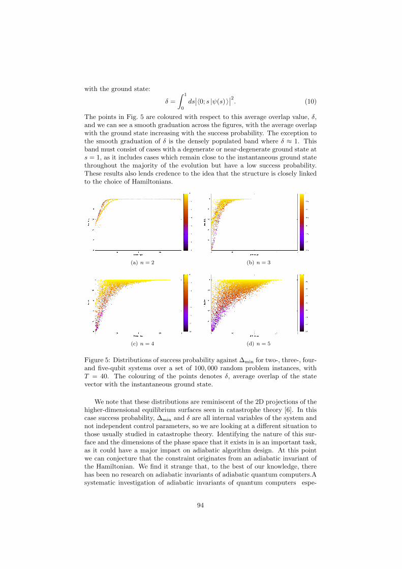
with the ground state:
δ =
∫ 1
0
ds∣∣〈0; s |ψ(s) 〉
∣∣2. (10)
The points in Fig. 5 are coloured with respect to this average overlap value, δ,and we can see a smooth graduation across the figures, with the average overlapwith the ground state increasing with the success probability. The exception tothe smooth graduation of δ is the densely populated band where δ ≈ 1. Thisband must consist of cases with a degenerate or near-degenerate ground state ats = 1, as it includes cases which remain close to the instantaneous ground statethroughout the majority of the evolution but have a low success probability.These results also lends credence to the idea that the structure is closely linkedto the choice of Hamiltonians.
(a) n = 2 (b) n = 3
(c) n = 4 (d) n = 5
Figure 5: Distributions of success probability against ∆min for two-, three-, four-and five-qubit systems over a set of 100, 000 random problem instances, withT = 40. The colouring of the points denotes δ, average overlap of the statevector with the instantaneous ground state.
We note that these distributions are reminiscent of the 2D projections of thehigher-dimensional equilibrium surfaces seen in catastrophe theory [6]. In thiscase success probability, ∆min and δ are all internal variables of the system andnot independent control parameters, so we are looking at a different situation tothose usually studied in catastrophe theory. Identifying the nature of this sur-face and the dimensions of the phase space that it exists in is an important task,as it could have a major impact on adiabatic algorithm design. At this pointwe can conjecture that the constraint originates from an adiabatic invariant ofthe Hamiltonian. We find it strange that, to the best of our knowledge, therehas been no research on adiabatic invariants of adiabatic quantum computers.Asystematic investigation of adiabatic invariants of quantum computers espe-
94

cially adiabatic and approximately adiabatic computers could yield importantinformation about their behaviour and make a major impact on the adiabaticalgorithm design.
5 Conclusion
We have shown that the relationship between the success probability and theminimum ground state gap may not be as straightforward as is often assumed.There is a rich structure of distinct sharp edges and densely-populated bandsin the distribution, particularly in smaller systems. A partial explanation hasbeen proposed, whereby this is the projection of a higher-dimensional surface;identification of the parameters governing this surface will guide understandingof the set of problems amenable to adiabatic quantum computing. We do notpropose a definitive explanation of the origin of this rich structure: this remainsan open question. However, we do suggest that there is some evidence thatsome of this structure could arise by our choice of Hamiltonians. We speculatethat a systematic investigation of adiabatic invariants of quantum computers— especially adiabatic and approximately adiabatic computers — could yieldimportant information about their behaviour and have a major impact on adi-abatic algorithm design.
References
[1] E. Farhi, J. Goldstone, S. Gutmann, and M. Sipser. Quantum computationby adiabatic evolution. quant-ph/0001106, 2000.
[2] A. M. Childs, E. Farhi, and J. Preskill. Robustness of adiabatic quantumcomputation. Phys. Rev. A, 65:012322, 2001.
[3] E. Farhi, J. Goldstone, S. Gutmann, J. Lapan, A. Lundgren, and D. Preda.A Quantum Adiabatic Evolution Algorithm Applied to Random Instancesof an NP-Complete Problem. Science, 292(5516):472–475, 2001.
[4] Arnab Das and Bikas K. Chakrabarti Quantum annealing and analog quan-tum computation, Rev. Mod. Phys. 80:1061-1081, 2008.
[5] J. R. Dormand and P. J. Prince. A family of embedded Runge-Kutta formu-lae. Journal of Computational and Applied Mathematics, 6(1):19–26, 1980.
[6] P. T. Saunders. An introduction to catastrophe theory. Cambridge UniversityPress, 1980.
95

Bibliography
[1] Richard P. Feynman. Simulating physics with computers. International Journal
of Theoretical Physics, VoL 21, Nos. 6/7, 1982.
[2] Peter W. Shor. Polynomial-time algorithms for prime factorization and dis-
crete logarithms on a quantum computer. SIAM J.Sci.Statist.Comput., 26:1484,
1997.
[3] Lov K. Grover. A fast quantum mechanical algorithm for database search. Pro-
ceedings, 28th Annual ACM Symposium on the Theory of Computing (STOC),
pages 212–219, 1996.
[4] David Deutsch. Quantum theory, the church-turing principle and the universal
quantum computer. Proceedings of the Royal Society of London A, 400:97–117,
1985.
[5] D Deutsch and R Jozsa. Rapid solution of problems by quantum computation.
Proc Roy Soc Lond A, 439:553–558, October 1992.
[6] Edward Farhi, Jeffrey Goldstone, Sam Gutmann, and Michael Sipser. Quantum
computation by adiabatic evolution. quant-ph/0001106, 2000.
[7] A.M. Childs, E. Farhi, and J. Preskill. Robustness of adiabatic quantum com-
putation. Phys. Rev. A, 65:012322, 2001.
[8] S. Ashhab, JR Johansson, and F. Nori. Decoherence in a scalable adiabatic
quantum computer. Phys. Rev. A, 74:052330, 2006.
[9] Jeremie Roland and Nicolas J. Cerf. Noise resistance of adiabatic quantum
computation using random matrix theory. Phys. Rev. A, 71:032330, 2005.
[10] D. Aharonov, W. van Dam, J. Kempe, Z. Landau, S. Lloyd, and O. Regev.
Adiabatic Quantum Computation is Equivalent to Standard Quantum Compu-
tation. quant-ph/0405098, 2004.
96

BIBLIOGRAPHY 97
[11] A. Mizel, D.A. Lidar, and M. Mitchell. Simple proof of equivalence between adi-
abatic quantum computation and the circuit model. Phys. Rev. Lett., 99:070502,
2007.
[12] M. H. S. Amin, Peter J. Love, and C. J. S. Truncik. Thermally assisted adiabatic
quantum computation. Phys. Rev. Lett., 100(6):060503, 2008.
[13] A. M. Turing. On computable numbers, with an application to the entschei-
dungsproblem. Proc. London Math. Soc., 2(42):230–265, 1936.
[14] David P. DiVincenzo. The physical implementation of quantum computation.
Arxiv preprint quant-ph/0002077, 2000.
[15] Michael A. Nielsen and Isaac L. Chuang. Quantum Computation and Quantum
Information. Cambridge University Press, 2000.
[16] B.H. Bransden and C.J. Joachain. Introduction To Quantum Mechanics. Long-
man Scientific & Technical, 1989.
[17] D.R. Mitchell, C. Adami, W. Lue, and C.P. Williams. Random matrix model
of adiabatic quantum computing. Physical Review A, 71(5):52324, 2005.
[18] M. Znidaric. Eigenlevel statistics of the quantum adiabatic algorithm. Physical
review. A, 72(5):52336–52336, 2005.
[19] W. Van Dam, M. Mosca, and U. Vazirani. How powerful is adiabatic quantum
computation? Foundations of Computer Science, Annual IEEE Symposium
on, 0:279, 2001.
[20] E. Farhi, J. Goldstone, and S. Gutmann. Quantum Adiabatic Evolution Algo-
rithms with Different Paths. ArXiv Quantum Physics e-prints, aug 2002.
[21] B. Altshuler, H. Krovi, and J. Roland. Adiabatic quantum optimization fails
for random instances of NP-complete problems. ArXiv e-prints, August 2009.
[22] Neil G. Dickson and M. H. S. Amin. Does adiabatic quantum optimization fail
for np-complete problems? Phys. Rev. Lett., 106(5):050502, Feb 2011.
[23] X. Peng, Z. Liao, N. Xu, G. Qin, X. Zhou, D. Suter, and J. Du. Quantum
Adiabatic Algorithm for Factorization and Its Experimental Implementation.
Physical Review Letters, 101(22):220405–+, November 2008.
[24] Jeremie Roland and Nicolas J. Cerf. Quantum search by local adiabatic evolu-
tion. Phys. Rev. A, 65(4):042308, Mar 2002.

BIBLIOGRAPHY 98
[25] Jeremie Roland and Nicolas J. Cerf. Adiabatic quantum search algorithm for
structured problems. Phys. Rev. A, 68(6):062312, Dec 2003.
[26] Matthias Steffen, Wim van Dam, Tad Hogg, Greg Breyta, and Isaac Chuang.
Experimental implementation of an adiabatic quantum optimization algorithm.
Phys. Rev. Lett., 90(6):067903, Feb 2003.
[27] Warren S. Warren. The usefulness of nmr quantum computing. Science,
277(5332):1688–1690, 1997.
[28] I. Chiorescu, Y. Nakamura, C. J. P. M. Harmans, and J. E. Mooij. Coherent
quantum dynamics of a superconducting flux qubit. Science, 299(5614):1869–
1871, 2003.
[29] E. Il’ichev, A. Yu Smirnov, M. Grajcar, A. Izmalkov, D. Born, N. Oukhanski,
Th Wagner, W. Krech, H. G. Meyer, and A. M. Zagoskin. Radio-frequency
method for investigation of quantum properties of superconducting structures.
FIZIKA NIZKIKH TEMPERATUR, 30:823, 2004.
[30] V. T. Petrashov, K. G. Chua, K. M. Marshall, R. Sh. Shaikhaidarov, and
J. T. Nicholls. Andreev probe of persistent current states in superconducting
quantum circuits. Phys. Rev. Lett., 95(14):147001, Sep 2005.
[31] S. H. W. van der Ploeg, A. Izmalkov, Alec Maassen van den Brink, U. Hubner,
M. Grajcar, E. Il’ichev, H.-G. Meyer, and A. M. Zagoskin. Controllable coupling
of superconducting flux qubits. Phys. Rev. Lett., 98(5):057004, Feb 2007.
[32] J. E. Mooij, T. P. Orlando, L. Levitov, Lin Tian, Caspar H. van der Wal, and
Seth Lloyd. Josephson persistent-current qubit. Science, 285(5430):1036–1039,
1999.
[33] S.H.W. van der Ploeg, A. Izmalkov, M. Grajcar, U. Hubner, S. Linzen,
S. Uchaikin, T. Wagner, A.Yu. Smirnov, A.M. van den Brink, M.H.S. Amin,
A.M. Zagoskin, E. Il’ichev, and H.-G. Meyer. Adiabatic quantum computation
with flux qubits, first experimental results. Applied Superconductivity, IEEE
Transactions on, 17(2):113 –119, june 2007.
[34] T. Lanting, A. J. Berkley, B. Bumble, P. Bunyk, A. Fung, J. Johansson,
A. Kaul, A. Kleinsasser, E. Ladizinsky, F. Maibaum, R. Harris, M. W. Johnson,
E. Tolkacheva, and M. H. S. Amin. Geometrical dependence of low frequency
noise in superconducting flux qubits. Phys. Rev. B, 79:060509, 2009.

BIBLIOGRAPHY 99
[35] R. Harris, J. Johansson, A. J. Berkley, M. W. Johnson, T. Lanting, Siyuan Han,
P. Bunyk, E. Ladizinsky, T. Oh, I. Perminov, E. Tolkacheva, S. Uchaikin, E. M.
Chapple, C. Enderud, C. Rich, M. Thom, J. Wang, B. Wilson, and G. Rose.
Experimental demonstration of a robust and scalable flux qubit. Phys. Rev. B,
81(13):134510, Apr 2010.
[36] S.; Yan F.; Yoshihara F.; Harrabi K.; Fitch G.; Cory D. G.; Nakamura Y.;
Tsai J.-S.; Oliver W.D. Bylander, J.; Gustavsson. Noise spectroscopy through
dynamical decoupling with a superconducting flux qubit. Nature Physics,
7:565570, 2011.
[37] Amin M.H.S. Gildert S. Lanting T. Hamze F. Dickson N. Harris R. Berkley
A.J. Johansson J. Bunyk-P. Chapple E.M. Enderud C. Hilton J.P. Karimi K.
Ladizinsky E. Ladizinsky N. Oh T. Perminov I. Rich C. Thom M.C. Tolkacheva
E. Truncik C.J.S. Uchaikin S. Wang J. Wilson B. Rose G. Johnson, M.W.
Quantum annealing with manufactured spins. Nature, 473(7346):194–198, 2011.
cited By (since 1996) 1.
[38] P. Pechukas. Distribution of energy eigenvalues in the irregular spectrum. Phys.
Rev. Lett., 51:943, 1983.
[39] T. Yukawa. New approach to the statistical properties of energy levels. Phys.
Rev. Lett., 54:1883, 1985.
[40] A. M. Zagoskin, S. Savel’ev, and Franco Nori. Modeling an adiabatic quantum
computer via an exact map to a gas of particles. Phys. Rev. Lett., 98(12):120503,
2007.
[41] Giuseppe E. Santoro, Roman Martoňak, Erio Tosatti, and Roberto Car.
Theory of Quantum Annealing of an Ising Spin Glass. Science, 295(5564):2427–
2430, 2002.
[42] L.D. Landau. Phys. Z. Sowjetunion 2, 46, 1932.
[43] C. Zener. Proc. R. Soc. London, Ser. A 137(696):696–702, 1932.
[44] E.C.G. Stueckelberg. Helv. Phys. Acta. 5, 369:369–422, 1932.
[45] M.L. Mehta. Random matrices. Academic Press, 2004.
[46] Hans-Jurgen Stockman. Quantum Chaos: an introduction. Cambridge Univer-
sity Press, 1999.

BIBLIOGRAPHY 100
[47] G. E. Uhlenbeck and L. S. Ornstein. On the theory of the brownian motion.
Phys. Rev., 36(5):823–841, Sep 1930.
[48] C.F. Gerald and P.O. Wheatley. Applied Numerical Analaysis (fifth edition).
Addison-Wesley, 1994.
[49] J. F. Shriner and G. E. Mitchell. Small sample size effects in statistical analyses
of eigenvalue distributions. Zeitschrift fr Physik A Hadrons and Nuclei, 342:53–
60, 1992. 10.1007/BF01294488.
[50] M Cullimore, M. Everitt, M. Ormerod, J. Samson, S Savel’ev, R. Wilson, and
A. Zagoskin. The relationship between minimum gap and success probability
in adiabatic quantum computing. ArXiv e-prints, 1107.4034, July 2011.
[51] A.M. Zagoskin. Quantum Engineering: Theory and Design of Quantum Coher-
ent Structures. Cambridge University Press, 2011.
[52] R. D. Wilson, A. M. Zagoskin, and S. Savel’ev. Noise-enhanced perfor-
mance of adiabatic quantum computing by lifting degeneracies. Phys. Rev.
A, 82(5):052328, Nov 2010.
[53] Yu. L. Klimontovich. Statistical Physics. Harwood, 1986.
[54] B.R. Young W.Y. Svrcek, D.P. Mahoney. A real-time approach to process con-
trol. Wiley, 2000.
[55] E.M. Lifshitz L.D. Landau. Mechanics. Butterworth-Heinemann, 1976.


