
The Price Impact and Survival of Irrational Traders -...
35
THE JOURNAL OF FINANCE • VOL. LXI, NO. 1 • FEBRUARY 2006 The Price Impact and Survival of Irrational Traders LEONID KOGAN, STEPHEN A. ROSS, JIANG WANG, and MARK M. WESTERFIELD ∗ ABSTRACT Milton Friedman argued that irrational traders will consistently lose money, will not survive, and, therefore, cannot influence long-run asset prices. Since his work, sur- vival and price impact have been assumed to be the same. In this paper, we demon- strate that survival and price impact are two independent concepts. The price impact of irrational traders does not rely on their long-run survival, and they can have a significant impact on asset prices even when their wealth becomes negligible. We also show that irrational traders’ portfolio policies can deviate from their limits long after the price process approaches its long-run limit. MOST NEOCLASSICAL ASSET PRICING MODELS RELY on the assumption that market participants (traders) are rational in the sense that they behave in ways that are consistent with the objective probabilities of the states of the economy (e.g., Radner (1972) and Lucas (1978)). In particular, they maximize expected utili- ties using the true probabilities of uncertain economic states. This approach is firmly rooted in the tradition of going from the normative to the positive in eco- nomics, yet there is mounting evidence that it is not descriptive of the observed behavior of the average market participant (see, e. g., Alpert and Raiffa (1982), Benartzi and Thaler (2001), Black (1986), Kahneman and Tversky (1979), and Odean (1998)). How the presence of traders with incorrect beliefs may affect the behavior of financial markets remains an open question. It has long been argued (see, e. g., Friedman (1953)) that irrational traders who use wrong beliefs cannot survive in a competitive market. Trading under the wrong beliefs causes them to lose their wealth. In the long run, it is the rational traders who control most of the wealth and determine asset prices. Using a partial equilibrium model, De Long et al. (1991) suggest that traders ∗ Kogan and Ross are from the Sloan School of Management, MIT and NBER; Wang is from the Sloan School of Management, MIT, NBER, and China Center for Financial Research; and Wester- field is from the Marshall School of Business, University of Southern California. The authors thank Phil Dybvig, David Easley, Ming Huang, Robert Stambaugh (the editor), Wei Xiong, an anonymous referee, and participants of the 2002 NBER Asset Pricing Summer Conference, the 2003 Econo- metric Society Meetings, the Liquidity Conference at the London School of Economics, the 2004 American Finance Association Meetings, the 2004 Society for Economic Dynamics Meetings, and seminars at Carnegie-Mellon, Duke, London Business School, MIT, NYU, University of Geneva, University of Lausanne, University of Maryland, University of Michigan, University of Oslo, University of Vienna, and the Wharton School for comments. The authors also thank the Interna- tional Center for FAME for the 2004 FAME Research Prize. 195
-
Upload
trannguyet -
Category
Documents
-
view
215 -
download
0
Transcript of The Price Impact and Survival of Irrational Traders -...

THE JOURNAL OF FINANCE • VOL. LXI, NO. 1 • FEBRUARY 2006
The Price Impact and Survivalof Irrational Traders
LEONID KOGAN, STEPHEN A. ROSS, JIANG WANG,
and MARK M. WESTERFIELD∗
ABSTRACT
Milton Friedman argued that irrational traders will consistently lose money, will not
survive, and, therefore, cannot influence long-run asset prices. Since his work, sur-
vival and price impact have been assumed to be the same. In this paper, we demon-
strate that survival and price impact are two independent concepts. The price impact
of irrational traders does not rely on their long-run survival, and they can have a
significant impact on asset prices even when their wealth becomes negligible. We also
show that irrational traders’ portfolio policies can deviate from their limits long after
the price process approaches its long-run limit.
MOST NEOCLASSICAL ASSET PRICING MODELS RELY on the assumption that marketparticipants (traders) are rational in the sense that they behave in ways thatare consistent with the objective probabilities of the states of the economy (e.g.,Radner (1972) and Lucas (1978)). In particular, they maximize expected utili-ties using the true probabilities of uncertain economic states. This approach isfirmly rooted in the tradition of going from the normative to the positive in eco-nomics, yet there is mounting evidence that it is not descriptive of the observedbehavior of the average market participant (see, e. g., Alpert and Raiffa (1982),Benartzi and Thaler (2001), Black (1986), Kahneman and Tversky (1979), andOdean (1998)). How the presence of traders with incorrect beliefs may affectthe behavior of financial markets remains an open question.
It has long been argued (see, e. g., Friedman (1953)) that irrational traderswho use wrong beliefs cannot survive in a competitive market. Trading underthe wrong beliefs causes them to lose their wealth. In the long run, it is therational traders who control most of the wealth and determine asset prices.Using a partial equilibrium model, De Long et al. (1991) suggest that traders
∗Kogan and Ross are from the Sloan School of Management, MIT and NBER; Wang is from the
Sloan School of Management, MIT, NBER, and China Center for Financial Research; and Wester-
field is from the Marshall School of Business, University of Southern California. The authors thank
Phil Dybvig, David Easley, Ming Huang, Robert Stambaugh (the editor), Wei Xiong, an anonymous
referee, and participants of the 2002 NBER Asset Pricing Summer Conference, the 2003 Econo-
metric Society Meetings, the Liquidity Conference at the London School of Economics, the 2004
American Finance Association Meetings, the 2004 Society for Economic Dynamics Meetings, and
seminars at Carnegie-Mellon, Duke, London Business School, MIT, NYU, University of Geneva,
University of Lausanne, University of Maryland, University of Michigan, University of Oslo,
University of Vienna, and the Wharton School for comments. The authors also thank the Interna-
tional Center for FAME for the 2004 FAME Research Prize.
195

196 The Journal of Finance
with wrong beliefs may survive in the long run because they may hold portfolioswith higher growth rates and, therefore, can eventually outgrow the rationaltraders.1 In contrast, in a general equilibrium setting, Sandroni (2000) andBlume and Easley (2001) show that with intermediate consumption, irrationaltraders do not survive in the long run.
The efficiency of financial markets is the principal motivation behind theinterest in the survival of irrational traders. If irrational traders impact as-set prices, then markets will not be efficient, either informationally or alloca-tionally. Implicitly, the discussion on survival is based on the assumption thatsurvival is a necessary condition for long-run price impact. It is thought thatirrational traders have to control a significant amount of wealth in order toaffect—or “infect”—prices with their irrational beliefs. In this paper, we showthat this assumption is false and that irrational traders can maintain a largeprice impact even as their relative wealth diminishes toward zero over time.
Our analysis is conducted with a parsimonious general equilibrium modelinhabited by both rational and irrational traders. Traders only care about theirterminal consumption. We are able to derive an explicit solution to the modeland obtain conditions under which the irrational traders can survive in thelong run in the sense that their share of the total wealth does not go to zeroover time. However, we show that even when irrational traders do not survive,with a negligible amount of wealth they can still exert significant influence onthe asset price over a long period of time.
Underlying this initially counterintuitive result is a solid economic intuition.Under incorrect beliefs, irrational traders express their views by taking posi-tions (bets) on extremely unlikely states of the economy. As a result, the stateprices of these extreme states can be significantly affected by the beliefs ofthe irrational traders, even with negligible wealth. In turn, these states, eventhough highly unlikely, can have a large contribution to current asset prices.This is especially true for states associated with extremely low levels of aggre-gate consumption in which the traders’ marginal utilities, and thus state prices,are very high. The beliefs of the irrational traders on these low probability buthigh marginal utility states can influence current asset prices and their dynam-ics. Furthermore, irrational traders need not take extreme positions in orderto influence prices. Our formal analysis clearly verifies this conceptual distinc-tion between the long-run price impact and the long-run survival of irrationaltraders.
The possibility that irrational traders may have a significant price impactwith a negligible share of wealth also has important implications for their sur-vival. In the partial equilibrium analysis of De Long et al. (1991), it is assumedthat when the irrational traders control only a negligible fraction of the totalwealth, they have no impact on asset prices. That is, asset prices behave as ifthe irrational traders are absent. Given the rationally determined prices, DeLong et al. then show that the wealth of irrational traders can grow at a fasterrate than the wealth of the rational traders, allowing the irrational traders to
1 See also Figlewski (1978) for a discussion on the notion of long-run survival.

The Price Impact and Survival of Irrational Traders 197
recover from their losses and survive in the long run. Although such an argu-ment is illuminating, it is based on unreliable premises. As we argue, irrationaltraders may still influence prices with diminishing wealth. Moreover, such apossibility can significantly affect the irrational traders’ portfolio policies inways that make recovery from losses difficult.
The paper proceeds as follows. In Section I, we provide a simple example toillustrate the possibility for an agent to affect asset prices with a negligiblewealth. Section II describes a canonical economy similar to that of Black andScholes (1973), but in the presence of irrational traders who have persistentlywrong beliefs about the economy; Section III describes the general equilibriumof this economy. Section IV treats the special case of logarithmic preferencesand demonstrates that even though irrational traders never survive in thiscase, they nevertheless can influence long-run asset prices. Sections V, VI, andVII analyze the survival of irrational traders, their price impact, and their port-folio policies, respectively. Section VIII discusses the importance of equilibriumeffects on the survival of irrational traders. Section IX concludes the paper witha short summary and some suggestions for future research. All proofs are givenin the Appendix.
I. An Example
We begin our analysis by considering a simple, static Arrow–Debreu economyand show that an agent with only a negligible amount of wealth can have asignificant impact on asset prices by using certain trading policies.
The economy has two dates, 0 and 1. It is endowed with one unit of a riskyasset, which pays dividend D only at date 1. The realization of D falls in [0, 1]with probability density p(D) = 2D, which is plotted in Figure 1(a).
There is a complete set of Arrow–Debreu securities traded in a competitivefinancial market at date 0. Shares of the stock and a risk-free bond with asure payoff of one at date 1, both of which are baskets of the Arrow–Debreu
Figure 1. Probability distribution of the stock dividend (the left panel), both the aggregate con-
sumption level (D) and the noise trader consumption (Cn) when the noise trader is present (the
middle panel), and the relative consumption of the noise trader (Cn/D, right panel). The upper
bound on the noise trader’s consumption, δ, is set to 0.2.

198 The Journal of Finance
securities, are also traded. We use the bond as the numeraire for the securityprices at date 0. Thus, the bond price is always one.
We first consider the economy when it is populated by a representative agent,with a logarithmic utility function over consumption at date 1, u(C) = log C. Itimmediately follows that C = D and the state price density (SPD), denoted byφ∗, is
φ∗(D) = a∗u′(D) = a∗
D,
where a∗ is a constant. The price of any payoff X is then given by
P = E[ X · φ∗ ].
In particular, the price of the bond is
B = E[ 1 · φ∗ ] =∫ 1
0
a∗
Dp(D) dD =
∫ 1
0
2a∗ dD = 2a∗ = 1,
which gives a∗ = 12. The price of the stock is then given by
S∗ = E[ D · φ∗] =∫ 1
0
D · 1
2Dp(D) dD =
∫ 1
0
D dD = 1
2.
Now we introduce to the economy another trader who has a negligible amountof wealth and who desires a particular consumption bundle. We denote thistrader by “N” and call him a noise trader. The noise trader demands consump-tion bundle
Cn = (1 − δ) min(δ, D), 0 < δ < 1
which is plotted in Figure 1(b). Figure 1(c) plots Cn as a fraction of the totalconsumption D. Since Cn ≤ δ(1 − δ), the wealth the noise trader needs to acquirethe consumption bundle, is
Wn = E[ Cn · φ ] ≤ E[ δ(1 − δ) · φ ] = δ(1 − δ) < δ,
where we use the fact that the bond price is one. The consumption for therepresentative agent (excluding the noise trade) is then C = D − Cn, also shownin Figure 1(b). The SPD in this case is
φ = au′(C) = aD − (1 − δ) min(δ, D)
.
Since the price of the bond is one, we have
B = E[ 1 · φ ] =∫ δ
0
aδD
(2D) dD +∫ 1
δ
aD − δ(1 − δ)
(2D) dD = 1,

The Price Impact and Survival of Irrational Traders 199
which gives
a = 1
4
{1 − δ
2+ 1
2δ(1 − δ)[ln(1 − δ + δ2) − 2 ln(δ)]
}−1
.
As noted above, the wealth needed to acquire the consumption bundle Cn, Wn,is less than δ, so it is small if δ is small. The stock price in the presence of thenoise trader is given by
S = E[ D · φ ] =∫ δ
0
Da
δD(2D) dD +
∫ 1
δ
Da
(1 − δ)δ(2D) dD
= a{1 + 3δ − 5δ2 + 2δ3 + 2δ2(1 − δ)2[ln(1 − δ + δ2) − 2 ln(δ)]} = 1
4+ O(δ),
where O(δ) denotes terms of order δ or higher. Thus, S/S∗ = 12
+ O(δ). We canmeasure the impact of the noise trade on the stock price by
1 − SS∗ = 1
2+ O(δ),
which remains nonnegligible even when δ, and therefore the amount of wealthcontrolled by the noise trader, approaches zero.
This is a stark result: A price-taking trader with negligible wealth can exertfinite influence on asset prices. The noise trader spends most of his wealthon consumption in low-dividend states. Given that the marginal utility of theother traders in these states is very high, the state prices for these states arealso high and, more importantly, a small change in the consumption level canchange the state prices significantly. As we show above, the wealth requiredfor the noise traders to finance their desired consumption profile is small, eventhough most of their consumption occurs in states with relatively high prices.
While the above example is rather simple, its intuition holds more generally.In the case of logarithmic preferences, the SPD is proportional to the ratio-nal trader’s marginal utility u′(C): φ = au′(C), where a is the proportionalityconstant. When the irrational trader is introduced into the economy and hepurchases ε units of state-contingent claims that pay off only when the aggre-gate consumption is C, the SPD will change by �φ ≈ −au′′(C)ε. The total costfor the purchase is w ≡ φε ≈ au′(C)ε when ε is small. Divided by the wealthspent by the irrational trader, we obtain the marginal change in the SPD,
�φ
w= u′′(C)
u′(C)= 1
C,
which is independent of ε. Clearly, in “bad” states, in which C is low (close tozero), irrational traders can have a large impact on the SPD with little wealthif they decide to bet on these states. Through their impact on the SPD in badstates, irrational traders can influence asset prices such as the prices of thestock and the bond. Given that the bond is used as a numeraire and its price is

200 The Journal of Finance
always one, this influence is captured in the stock price, S = E[ D · φ], as shownabove.
Our example clearly demonstrates the possibility of influencing asset priceswith little wealth. The remaining question is whether such a situation canarise in more realistic settings. In particular, for our purpose in this paper,can the irrational traders with incorrect beliefs maintain a significant priceimpact even as their relative wealth diminishes from investment losses in themarket? In the remainder of the paper, we use a canonical model to addressthese questions.
II. The Model
We consider a standard setting similar to that of Black and Scholes (1973).For simplicity, we make the model parsimonious.
A. Information Structure
The economy has a finite horizon and evolves in continuous time. Uncertaintyis described by a one-dimensional, standard Brownian motion Bt for 0 ≤ t ≤ T,defined on a complete probability space (�, F, P), where F is the augmentedfiltration generated by Bt.
B. The Financial Market
There is a single share of a risky asset in the economy, the stock, which paysa terminal dividend payment DT at time T, determined by the process
dDt = Dt(μ dt + σ dBt), (1)
where D0 = 1 and σ > 0. There is also a zero-coupon bond available in zero netsupply. Each unit of the bond makes a sure payment of one at time T. We usethe risk-free bond as the numeraire and denote the price of the stock at timet by St.
C. Endowments
There are two competitive traders in the economy, each endowed with a halfshare of the stock (and none of the bond) at time zero.
D. Trading Strategies
The financial market is frictionless and has no constraints on lending andborrowing. Traders’ trading strategies satisfy the standard integrability condi-tion used to avoid pathologies,
E0
[∫ T
0
θ2t d 〈S〉t
]< ∞, (2)

The Price Impact and Survival of Irrational Traders 201
where θt is the number of stock shares held in the portfolio at time t and 〈S〉tis the quadratic variation process of St (see, e. g., Duffie and Huang (1985) andHarrison and Kreps (1979)).
E. Preferences and Beliefs
Both traders have constant relative-risk aversion utility over their consump-tion at time T,
1
1 − γC1−γ
T , γ ≥ 1.
For ease of exposition, we only consider the cases in which γ ≥ 1. The caseswhen 0 < γ < 1 can be analyzed similarly and the results are similar in spirit.
Standard aggregation results imply that each trader in our model can actu-ally represent a collection of traders with the same preferences. This providesa justification for our competitive assumption for each of the traders. The firsttrader, the rational trader, knows the true probability measure P and maxi-mizes expected utility
EP0
[1
1 − γC1−γ
r,T
], (3)
where the subscript r denotes quantities associated with the rational trader.The second trader, the irrational trader, believes incorrectly that the probabilitymeasure is Q, under which
dBt = (ση) dt + dBQt (4)
and, hence
dDt = Dt[(
μ + σ 2η)
dt + σdBQt
], (5)
where BQt is the standard Brownian motion under the measure Q and η is a
constant, parameterizing the degree of irrationality of the irrational trader.When η is positive, the irrational trader is optimistic about the prospects of theeconomy and thus overestimates the rate of growth of the aggregate endow-ment. Conversely, a negative η corresponds to a pessimistic irrational trader.The irrational trader maximizes expected utility using belief Q:
EQ0
[1
1 − γC1−γ
n,T
], (6)
where the subscript n denotes quantities associated with the irrational trader.Because η is assumed to be constant, the probability measure of the irrational
trader Q is absolutely continuous with respect to the objective measure P, thatis, both traders agree on zero-probability events. Let ξt ≡ (dQ/dP)t denote thedensity (Radon–Nikodym derivative) of the probability measure Q with respectto P,
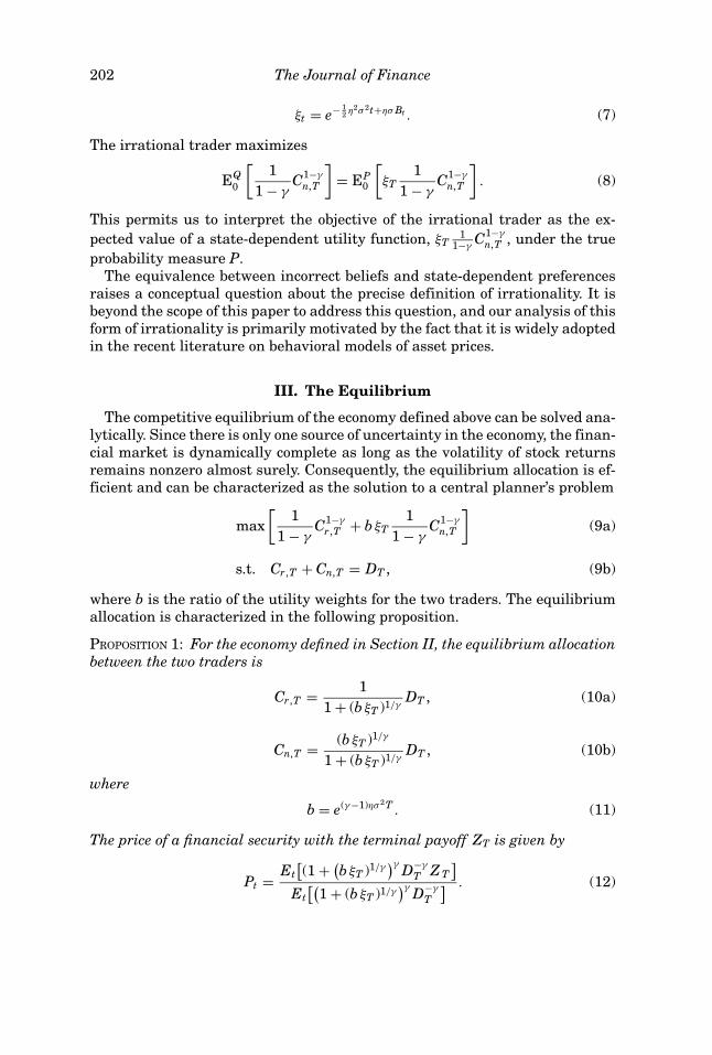
202 The Journal of Finance
ξt = e− 12η2σ 2t+ησ Bt . (7)
The irrational trader maximizes
EQ0
[1
1 − γC1−γ
n,T
]= EP
0
[ξT
1
1 − γC1−γ
n,T
]. (8)
This permits us to interpret the objective of the irrational trader as the ex-
pected value of a state-dependent utility function, ξT1
1−γC1−γ
n,T , under the true
probability measure P.The equivalence between incorrect beliefs and state-dependent preferences
raises a conceptual question about the precise definition of irrationality. It isbeyond the scope of this paper to address this question, and our analysis of thisform of irrationality is primarily motivated by the fact that it is widely adoptedin the recent literature on behavioral models of asset prices.
III. The Equilibrium
The competitive equilibrium of the economy defined above can be solved ana-lytically. Since there is only one source of uncertainty in the economy, the finan-cial market is dynamically complete as long as the volatility of stock returnsremains nonzero almost surely. Consequently, the equilibrium allocation is ef-ficient and can be characterized as the solution to a central planner’s problem
max
[1
1 − γC1−γ
r,T + b ξT1
1 − γC1−γ
n,T
](9a)
s.t. Cr,T + Cn,T = DT , (9b)
where b is the ratio of the utility weights for the two traders. The equilibriumallocation is characterized in the following proposition.
PROPOSITION 1: For the economy defined in Section II, the equilibrium allocationbetween the two traders is
Cr,T = 1
1 + (b ξT )1/γDT , (10a)
Cn,T = (b ξT )1/γ
1 + (b ξT )1/γDT , (10b)
where
b = e(γ−1)ησ 2T . (11)
The price of a financial security with the terminal payoff ZT is given by
Pt = Et[(1 + (
b ξT )1/γ)γ D−γ
T Z T]
Et[(
1 + (b ξT )1/γ)γ D−γ
T
] . (12)

The Price Impact and Survival of Irrational Traders 203
For the stock, ZT = DT and its return volatility is bounded between σ andσ (1 + |η|).
Since the instantaneous volatility of stock returns is bounded below by σ , thestock and the bond dynamically complete the financial market. In the limitingcases in which only the rational or the irrational trader is present, the stockprices, denoted by S∗
t and S∗∗t , respectively, are given by
S∗t = e(μ/σ 2−γ )σ 2T+ 1
2(2γ−1)σ 2t+σ Bt (13a)
S∗∗t = e(μ/σ 2−γ+η)σ 2T+ 1
2[(2γ−1)−2η]σ 2t+σ Bt = S∗
t eησ 2(T−t). (13b)
We will use this equilibrium model to analyze the survival and extinctionof the traders. We employ the following common definition of extinction, and,conversely, of survival.
DEFINITION 1: The irrational trader is said to experience relative extinction inthe long run if
limT→∞
Cn,T
Cr,T= 0 a.s. (14)
The relative extinction of the rational trader can be defined symmetrically. Atrader is said to survive relatively in the long run if relative extinction does notoccur.
In the above definition and throughout the paper, all limits are understood tobe almost sure (under the true probability measure P) unless specifically statedotherwise.
In our model, the final wealth of each trader equals their terminal consump-tion. Thus, the definition of survival and extinction is equivalent to a similardefinition in terms of wealth.
IV. Logarithmic Preferences
We first consider the case in which both the rational and the irrational tradershave logarithmic preferences. We have the following result:
PROPOSITION 2: Suppose η �= 0. For γ = 1, the irrational trader never survives.
This result is immediate. For γ = 1, the rational trader holds the portfolio withmaximum expected growth (see, e.g., Hakansson (1971)). Any deviation in be-liefs from the true probability causes the irrational trader to move away fromthe maximum growth portfolio, which leads to his long-run relative extinction.
Our interest here, however, is not in the survival of the irrational trader,but rather in the impact of irrationality on the long-run stock price. Underlogarithmic preferences, b = 1, and from Proposition 1, the stock price is
St = 1 + ξt
Et[(1 + ξT )/DT
] = 1 + ξt
1 + e−ησ 2(T−t)ξtS∗
t , (15)
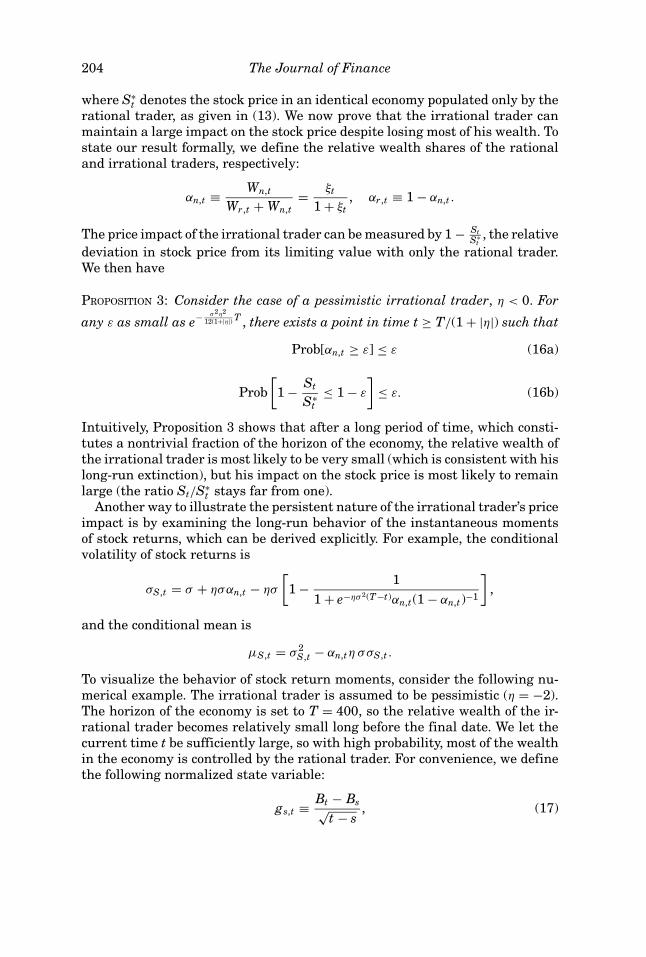
204 The Journal of Finance
where S∗t denotes the stock price in an identical economy populated only by the
rational trader, as given in (13). We now prove that the irrational trader canmaintain a large impact on the stock price despite losing most of his wealth. Tostate our result formally, we define the relative wealth shares of the rationaland irrational traders, respectively:
αn,t ≡ Wn,t
Wr,t + Wn,t= ξt
1 + ξt, αr,t ≡ 1 − αn,t .
The price impact of the irrational trader can be measured by 1 − StS∗
t, the relative
deviation in stock price from its limiting value with only the rational trader.We then have
PROPOSITION 3: Consider the case of a pessimistic irrational trader, η < 0. For
any ε as small as e− σ2η2
12(1+|η|) T , there exists a point in time t ≥ T/(1 + |η|) such that
Prob[αn,t ≥ ε] ≤ ε (16a)
Prob
[1 − St
S∗t
≤ 1 − ε
]≤ ε. (16b)
Intuitively, Proposition 3 shows that after a long period of time, which consti-tutes a nontrivial fraction of the horizon of the economy, the relative wealth ofthe irrational trader is most likely to be very small (which is consistent with hislong-run extinction), but his impact on the stock price is most likely to remainlarge (the ratio St/S∗
t stays far from one).Another way to illustrate the persistent nature of the irrational trader’s price
impact is by examining the long-run behavior of the instantaneous momentsof stock returns, which can be derived explicitly. For example, the conditionalvolatility of stock returns is
σS,t = σ + ησαn,t − ησ
[1 − 1
1 + e−ησ 2(T−t)αn,t(1 − αn,t)−1
],
and the conditional mean is
μS,t = σ 2S,t − αn,tη σσS,t .
To visualize the behavior of stock return moments, consider the following nu-merical example. The irrational trader is assumed to be pessimistic (η = −2).The horizon of the economy is set to T = 400, so the relative wealth of the ir-rational trader becomes relatively small long before the final date. We let thecurrent time t be sufficiently large, so with high probability, most of the wealthin the economy is controlled by the rational trader. For convenience, we definethe following normalized state variable:
gs,t ≡ Bt − Bs√t − s
, (17)

The Price Impact and Survival of Irrational Traders 205
5 4 3 2 1 0 1 2 3 4 50
0.2
0.4
0.6
0.8
1
μt,
S / σ
t,S
Sharpe ratio
5 4 3 2 1 0 1 2 3 4 50
0.2
0.4
5 4 3 2 1 0 1 2 3 4 50
0.2
0.4
0.6
0.8
1
Normalized state, t 1/2 Bt
αt,r
Wealth distribution
5 4 3 2 1 0 1 2 3 4 50
0.2
0.4
Figure 2. The conditional Sharpe ratio of stock returns μS,t/σS,t and the fraction of wealth con-
trolled by the rational trader αr,t = Wr,t/(Wr,t + Wn,t) are plotted against the normalized state
variable g0,t ≡ Bt/√
t. The shaded area is the probability density function of the normalized state
variable (vertical axis on the right). The average dividend growth rate is μ = 0.05, the volatility of
dividend growth is σ = 0.15, the bias of irrational trader’s beliefs is η = −2, the terminal date is
T = 400, and both agents have unit risk aversion, γ = 1. The current time is t = 150.
where s < t. It is easy to show that gs,t is the unanticipated dividend growthnormalized by its standard deviation, which has a standard normal distribu-tion. Figure 2 plots the Sharpe ratio of instantaneous stock returns and thewealth distribution between the two traders at t = 150 against the normalizedstate variable g0,t. The probability density for g0,t is illustrated by the shadedarea (with the vertical axis on the right). The bottom panel of Figure 2 showsthat with almost probability one, all the wealth of the economy is controlled bythe rational trader at this time. Yet, as the top panel of the figure shows, theconditional Sharpe ratio of stock returns is very different from σ , which is theratio’s value in the economy populated only by the rational trader. In particular,over a large range of values of dividends, the conditional Sharpe ratio of returnsis approximately equal to σ (1 − η) �= σ .
Figure 3 provides a complementary illustration. It shows the most likely pathover time (the path with highest probability) for the irrational trader’s wealthshare and the Sharpe ratio of stock returns. In fact, the irrational trader’s

206 The Journal of Finance
0 50 100 150 200 250 300 350 4000.1
0.2
0.3
0.4
0.5
μt,
S / σ
t,S
Sharpe ratio
0 50 100 150 200 250 300 350 4000
0.2
0.4
0.6
0.8
1
Time, t
αt,
n
Wealth distribution
Figure 3. The maximum likelihood path of the irrational trader’s wealth share, αn,t = Wn,t/(Wr,t +Wn,t), and the Sharpe ratio, μS,t/σS,t. The average dividend growth rate is μ = 0.05, the volatility
of dividend growth is σ = 0.15, the bias of irrational trader’s beliefs is η = −2, the terminal date is
T = 400, and both agents have unit risk aversion, γ = 1.
wealth share diminishes to zero exponentially while his price impact diminishesat a much slower rate. The Sharpe ratio stays away from its level in an economywithout an irrational trader for an extended period of time before eventuallyconverging to the limiting value.
In order to better understand how the irrational trader can exert influence onthe stock price despite having negligible wealth, we examine how his presenceaffects the SPD. The left panels of Figure 4 plot the relative consumption sharesof the rational and the irrational traders at two different times, t = 0 and t =25, as a function of the normalized state variable gt,T, that is, the normalizedunanticipated dividend growth from t to T defined in (17). At each date, thestate of the economy is conditioned on Bt = 0, the most likely state. For t = 0, theirrational trader owns half of the economy. But at η = −4, he is very pessimisticand bets on states of low dividends (states toward the left end of the horizontalaxis). This is shown in the top left panel of Figure 4. The dashed line plots histerminal consumption for different states of the economy. It is worth pointingout that the consumption choice of the irrational trader in this economy is

The Price Impact and Survival of Irrational Traders 207
5 0 50
0.2
0.4
0.6
0.8
1
noit
pm
usn
oC
t = 0
5 0 50
0.2
0.4
5 0 510
0
10
20t = 0
DP
S
5 0 50
0.2
0.4
5 0 50
0.2
0.4
0.6
0.8
1
Normalized state, (T t) 1/2 (BT
Bt)
noit
pm
usn
oC
t = 25
5 0 50
0.2
0.4
5 0 510
0
10
20t = 25
DP
S
Normalized state, (T t) 1/2 (BT
Bt)
5 0 50
0.2
0.4
Figure 4. The terminal consumption of the rational and irrational traders as a fraction of the
total consumption and the state price density (SPD) in different terminal states of the economy at
different times. The average growth rate of the dividend is set at μ = 0.05, the volatility of dividend
growth is σ = 0.15, the bias of irrational trader’s beliefs is η = −4, the terminal date is T = 50, and
both agents have unit risk aversion, γ = 1. The horizontal axis in all panels is the normalized state
variable gt,T ≡ (BT − Bt )/√
T − t, which has a standard normal distribution with zero mean and
unit variance, which is shown by the shaded area (vertical axis on the right). In the two panels
on the left, the terminal consumption for the rational trader (the solid line) and the irrational
trader (the dotted line) are plotted against the normalized state variable at times t = 0 and t = 25,
respectively, when Bt = 0. In the two panels on the right, the dashed line plots the logarithm of the
SPD at times t = 0 and t = 25, respectively, which is ln{[(1 + ξT )/DT ]/Et [(1 + ξT )/DT ]}. The solid
line plots the logarithm of the SPD in the economy populated only by the rational traders, which
is ln{D−1T /Et [D−1
T ]}.
similar to that in the simple one-period economy we consider in Section I, asshown in Figure 1(c), where the irrational trader consumes a share of 1 − δ
of the aggregate endowment in states with low dividends, and a much smallershare in other states. This explains why in both economies, the irrational tradercan exert significant influence on prices despite being left with relatively littlewealth.
Over time, the “bad” states become less likely and the irrational trader’s betsbecome less valuable. Thus, his wealth decreases. At t = 25 and Bt = 0, these

208 The Journal of Finance
bad states become extremely unlikely, and the irrational trader has lost most ofhis wealth. His wealth as fraction of total wealth has fallen from 0.5 at t = 0 to0.01. As shown in the bottom left panel of Figure 4, going forward, the irrationaltrader consumes a nontrivial fraction of the total wealth only in the extremestates toward the left end of the horizontal axis. The probability of these states,as shown by the shaded area, becomes very small.
In the two panels on the right of Figure 4, we plot the state SPD against thenormalized state variable gt,T at the two times, t = 0 and t = 25, conditionedagain on Bt = 0. With logarithmic preferences, the equilibrium SPD at timet is given by
φt ≡ (1 + ξT )D−1T
Et[(1 + ξT )D−1
T
] , (18)
which is represented by the dashed line in each of the two panels. The solidline plots the SPD when the economy is populated only by the rational traders,which can be obtained by setting ξT = 0 in the above expression for φt. Thetop panel gives the SPD at t = 0. At this point, the irrational trader has a halfshare of the total wealth and his portfolio policy has a significant influence onthe SPD over the whole range. In particular, being pessimistic, he is effectivelybetting on the bad states, which causes the SPD to increase for the bad statesand decrease for the good states. This is shown by the difference between thedashed line, the SPD in the presence of the irrational trader, and the solid line,the SPD without the irrational trader. As time passes, the irrational trader’swealth dwindles and his influence on the SPD diminishes quickly for most ofthe states, as the bottom panel for t = 25 shows. However, for the extremelybad states, his influence remains significant because he is still betting heavilyon these states.
We can show that the price impact of the irrational trader with negligiblewealth does not rely on excessive leverage. The fraction of the irrational trader’swealth invested in the stock is given by σS,t + ησ (1 − αn,t), which is bounded inabsolute value by σ (1 + 2|η|). The irrational trader can make bets on stateswith a low aggregate endowment not by taking extreme portfolio positions, butrather by underweighting the stock in his portfolio over long periods of time.
The simple case of logarithmic preferences developed above clearly showsthat survival and price impact are in general not equivalent. In particular,survival is not a necessary condition for the irrational trader to influence long-run prices, and depending on their beliefs, irrational traders can maintain asignificant price impact even as their wealth becomes negligible over time.
In the remaining sections, we consider the general case of γ �= 1 and analyzethe survival of the irrational trader, his price impact, and his portfolio choices.
V. Survival
In the case of logarithmic preferences, the irrational trader does not survivein the long run simply because his portfolio grows more slowly than the maxi-mum growth rate, the rate achieved by the rational trader. For the coefficient

The Price Impact and Survival of Irrational Traders 209
of relative-risk aversion different from one, however, the rational trader nolonger holds the optimal growth portfolio, and under an incorrect belief, theirrational trader may end up holding a portfolio that is closer to the optimalgrowth portfolio and thus his wealth may grow more rapidly. This is the ar-gument put forward by De Long et al. using a partial equilibrium setting. Inthis section, we examine the long-run survival of the irrational trader in ourgeneral equilibrium setting.
From the competitive equilibrium derived in Section III, we have the follow-ing result:
PROPOSITION 4: Suppose η �= 0. Let η = 2(γ − 1). For γ > 1 and η �= η , only oneof the traders survives in the long run. In particular, we have
Pessimistic irrational trader: η < 0 ⇒ Rational trader survives,
Moderately optimistic irrational trader: 0 < η < η ⇒ Irrational trader survives,
Strongly optimistic irrational trader: η > η ⇒ Rational trader survives.
(19)
For η = η , both rational and irrational traders survive.
For γ > 1, Proposition 4 identifies three distinct regions in the parameterspace as shown in Figure 5. For η < 0, the irrational trader is pessimistic anddoes not survive in the long run. For 0 < η < η , the irrational trader is mod-erately optimistic and survives in the long run while the rational trader doesnot. For η > η , the irrational trader is strongly optimistic and does not survive.Clearly, other than the knife-edge case (η = η ), only one of the traders survives.
In order to gain more insight into what determines the survival of each typeof trader, we examine the terminal wealth (consumption) profile of both types.The two panels on the left in Figure 6 show the two traders’ terminal wealthprofiles for two values of T (10 and 30) when the irrational trader is pessimistic.The solid line shows the terminal wealth share of the rational trader and thedashed line shows that for the irrational trader.
As expected, the rational trader ends up with more wealth in good statesof the economy (when the dividend is high) while the irrational trader, beingpessimistic, ends up with more wealth in the bad states of the economy. Asthe horizon increases, the irrational trader ends up with nontrivial wealth inmore extreme and less likely low-dividend states. When the irrational traderis mildly optimistic, the situation is different. His impact on the prices makesthe bad states (i.e., the low dividend states) cheaper than the good states. Thisinduces the rational trader to accumulate more wealth in the bad states bygiving up wealth in the good states, including those with high probabilities. Asa result, the irrational trader is more likely to end up with more wealth. Whenstrongly optimistic, the irrational trader ends up accumulating wealth in veryunlikely, good states by giving up wealth in most other states, which leads tohis extinction in the long run.

210 The Journal of Finance
1 1.5 22
1
0
1
2sr
ed
art la
noit
arrI′
,feil
eb
η
Risk aversion, γ
N
R
R
Figure 5. The survival of rational and irrational traders for different values of η and γ . For each
region in the parameter space, we document which of the traders survives in the long run. “R”
means that survival of the rational trader is guaranteed inside the region, “N” corresponds to the
irrational trader.
It is important to recognize that our results on the long-run survival of irra-tional traders are obtained in the absence of intermediate consumption. In otherwords, these results are primarily driven by the portfolio choices of differenttraders in the market and their impact on prices. This allows us to focus on howirrational beliefs influence the behavior of traders and how they alone affecttheir wealth evolution. When intermediate consumption is allowed, traders’consumption policies will also be affected by their beliefs, which can signifi-cantly affect their wealth accumulation as well. The net impact of irrationalbelief on a trader’s wealth evolution depends on how it affects his portfoliochoice and his consumption choice. Using an infinite horizon setting with in-termediate consumption, Blume and Easley (2001) and Sandroni (2000) showthat traders with (persistently) irrational beliefs will not survive while traderswith rational beliefs will. Their analyses clearly show that the influence of in-correct beliefs on the irrational traders’ consumption policies can reduce theirchances of survival. However, this result relies on several conditions imposedon the traders’ preferences and the aggregate endowment. For example, theyrequire that aggregate endowment be bounded above and below, away fromzero. When these bounds are not imposed, as is the case in this paper, traders

The Price Impact and Survival of Irrational Traders 211
5 0 50
0.2
0.4
0.6
0.8
1η = 0.3 η*
01 =
T ,noitpmusno
C
5 0 50
0.2
0.4
5 0 50
0.2
0.4
0.6
0.8
1
Normalized state, T 1/2 BT
03 =
T ,noitpmusno
C
5 0 50
0.2
0.4
5 0 50
0.2
0.4
0.6
0.8
1η = 0.5 η*
5 0 50
0.2
0.4
5 0 50
0.2
0.4
0.6
0.8
1
Normalized state, T 1/2 BT
5 0 50
0.2
0.4
5 0 50
0.2
0.4
0.6
0.8
1η = 2 η*
5 0 50
0.2
0.4
5 0 50
0.2
0.4
0.6
0.8
1
Normalized state, T 1/2 BT
5 0 50
0.2
0.4
Figure 6. The terminal consumption of rational and irrational traders for different horizons T.
We consider two values of T, 10 and 30, respectively. The average dividend growth rate is μ = 0.12,
the volatility of dividend-growth is σ = 0.18, and both traders have relative-risk aversion γ = 5.
We consider three distinctive cases for the irrational trader’s belief: (1) pessimistic, η = −0.3η ,
(2) moderately optimistic, η = 0.5η , and (3) strongly optimistic, η = 2η , where η = 2(γ − 1). The
horizontal axis in all panels is the normalized value of the terminal dividend, that is, [ln DT −(μ − 1
2σ 2)T ]/(σ
√T ), which has a standard normal distribution with zero mean and unit variance,
shown by the shaded area (vertical axis on the right). The two panels on the left show the terminal
consumption, as a fraction of the total consumption, of the rational trader (solid line) and the
irrational trader (dashed line) with a pessimistic belief, that is, Cr,T/DT and Cn,T/DT , for the two
values of the horizon, T = 10 and T = 30, respectively. The two panels in the middle and on the
right show the terminal consumption, as a fraction of the total consumption, of the rational trader
and the irrational trader, with a moderately and strongly optimistic beliefs for the two values of
T, respectively.
with rational beliefs may not always survive while traders with irrational be-liefs may.2 To provide a comprehensive analysis of the survival conditions withintermediate consumption is beyond the scope of this paper and is left forfuture research. But, it suffices to say that even with intermediate consump-tion, the long-run survival of irrational traders is possible in the absence offurther restrictions on preferences and/or endowments.
2 In a simple case considered by Wang (1996), even among rational traders, survival depends on
preferences. In our setting, we do not impose any upper or positive lower bounds on endowments.
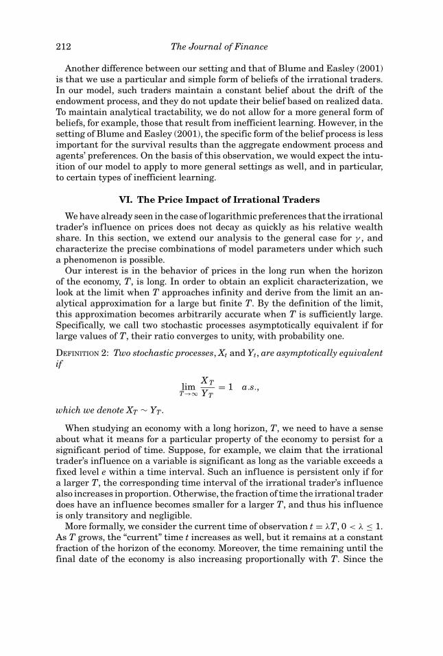
212 The Journal of Finance
Another difference between our setting and that of Blume and Easley (2001)is that we use a particular and simple form of beliefs of the irrational traders.In our model, such traders maintain a constant belief about the drift of theendowment process, and they do not update their belief based on realized data.To maintain analytical tractability, we do not allow for a more general form ofbeliefs, for example, those that result from inefficient learning. However, in thesetting of Blume and Easley (2001), the specific form of the belief process is lessimportant for the survival results than the aggregate endowment process andagents’ preferences. On the basis of this observation, we would expect the intu-ition of our model to apply to more general settings as well, and in particular,to certain types of inefficient learning.
VI. The Price Impact of Irrational Traders
We have already seen in the case of logarithmic preferences that the irrationaltrader’s influence on prices does not decay as quickly as his relative wealthshare. In this section, we extend our analysis to the general case for γ , andcharacterize the precise combinations of model parameters under which sucha phenomenon is possible.
Our interest is in the behavior of prices in the long run when the horizonof the economy, T, is long. In order to obtain an explicit characterization, welook at the limit when T approaches infinity and derive from the limit an an-alytical approximation for a large but finite T. By the definition of the limit,this approximation becomes arbitrarily accurate when T is sufficiently large.Specifically, we call two stochastic processes asymptotically equivalent if forlarge values of T, their ratio converges to unity, with probability one.
DEFINITION 2: Two stochastic processes, Xt and Yt, are asymptotically equivalentif
limT→∞
X T
YT= 1 a.s.,
which we denote XT ∼ YT.
When studying an economy with a long horizon, T, we need to have a senseabout what it means for a particular property of the economy to persist for asignificant period of time. Suppose, for example, we claim that the irrationaltrader’s influence on a variable is significant as long as the variable exceeds afixed level e within a time interval. Such an influence is persistent only if fora larger T, the corresponding time interval of the irrational trader’s influencealso increases in proportion. Otherwise, the fraction of time the irrational traderdoes have an influence becomes smaller for a larger T, and thus his influenceis only transitory and negligible.
More formally, we consider the current time of observation t = λT, 0 < λ ≤ 1.As T grows, the “current” time t increases as well, but it remains at a constantfraction of the horizon of the economy. Moreover, the time remaining until thefinal date of the economy is also increasing proportionally with T. Since the

The Price Impact and Survival of Irrational Traders 213
properties of the equilibrium prices and quantities depend on how much timeis remaining until the final date, they depend on λ.
We define three values of λ to help us characterize points of change in thelimiting behavior:
λS ≡ 2
2γ − η, λr ≡ η
(γ − 1)(2γ − η), λn ≡ η
η(γ + 1) − 2γ (γ − 1). (20)
It is easy to verify that for η < η , 0 < λS ≤ 1; for 0 < η ≤ η , 0 < λr ≤ 1; and forη < 0 or η > η , 0 < λn ≤ 1. The limiting behavior of the stock price process canbe characterized as follows.
PROPOSITION 5: At t = λT, the stock price behaves as follows:
Case 1: Pessimistic irrational trader (η < 0):
St ∼{
S∗t eη[σ 2T + 1
2(η−2γ )σ 2t − σ Bt ], 0 < λ < λS
S∗t , λS < λ ≤ 1.
(21)
Case 2: Moderately optimistic irrational trader (0 < η < η ):
St ∼{
S∗t eη[(γ−1− 1
2η)σ 2t + σ Bt ], 0 < λ < λS
S∗∗t , λS < λ ≤ 1.
(22)
Case 3: Strongly optimistic irrational trader (η < η):
St ∼ S∗t . (23)
The values of the stock price in homogeneous economies, S∗t and S∗∗
t , are givenin equation (13). The asymptotic values of the instantaneous moments of stockreturns are equal to the moments of the corresponding asymptotic expressionsfor stock prices above.
Observe that in the first two cases, when the irrational trader is pessimisticor moderately optimistic, the stock price process does not converge quickly to itsvalue in the economy populated exclusively by the rational trader who survivesin the long run. Instead, over long periods of time, that is, for t between 0 andλST, the stock price process is affected by the presence of both traders. Thiscan occur even when the wealth of the irrational trader becomes negligiblelong before λST.3 Thus, we have generalized the results obtained in the contextof a log-utility economy. A trader can control an asymptotically infinitesimalfraction of the total wealth and yet exerts a nonnegligible effect on the stockprice. In other words, convergence to zero in wealth does not readily implyconvergence to zero in price impact.
3 For brevity, we omit the discussion of wealth distribution over time. Interested readers can refer
to our working paper, Kogan et al. (2003), where we show that for Cases 1 and 3, the irrational
trader’s wealth is asymptotically negligible for any time λT with λ < λS.

214 The Journal of Finance
VII. Portfolio Policies
Proposition 5 in the previous section established the possibility that a traderwhose wealth diminishes over time can have a persistent impact on assetprices. In this section, we study the traders’ portfolio policies. In particular,we show that convergence in the price process does not lead to immediate con-vergence in policies, which is another and somewhat subtle channel throughwhich traders with asymptotically infinitesimal wealth may affect the long-runbehavior of the economy. Moreover, by characterizing the portfolio policy, onegains an alternative view on long-run survival in equilibrium that is comple-mentary to the analysis of state-contingent consumption choices in Sections IVand V.
Expressions for portfolio policies are not available in closed form. However,using an argument similar to that in the proof of the bound on stock pricevolatility in Proposition 1, we can establish the following result:
PROPOSITION 6: For both traders, their portfolio weight in the stock, denoted byw, is bounded:
|w| ≤ 1 + |η|(γ + 1)/γ. (24)
The bound on the traders’ portfolio holdings is important for our results. Itexplicitly shows that the price impact of the irrational trader with negligiblewealth does not rely on excessive leverage. It also implies that our long-runsurvival results do not rely on the use of high leverage by the traders. Oursolution for the equilibrium remains valid even if traders are constrained intheir portfolio choices, as long as the constraint is sufficiently relaxed to allowfor w = ±[1 + |η|(γ + 1)/γ ].
To analyze the traders’ portfolio policies in more detail, we decompose atrader’s stock demand into two components, the myopic component and thehedging component. The sum of the two gives the trader’s total stock demand.We have the following proposition.
PROPOSITION 7: At t = λT, the individual stock holdings behave as follows:
Case 1: Pessimistic irrational trader (η < 0):4
wr,t ∼
⎧⎪⎪⎨⎪⎪⎩(myopic) (hedging) (total)
γ − η
γ (1 − η)− (γ − 1)η
γ (1 − η)= 1, 0 < λ < λS
1 + 0 = 1, λS < λ ≤ 1.
(25a)
4 The limit of the irrational trader’s portfolio policy for values of λ ∈ [min(λn, λS), max(λn, λS)] can
be characterized as explicitly as well, but the results depend on the ordering between λn and λS,
which in turn is determined by the values of model parameters. We omit these results to simplify the
exposition.

The Price Impact and Survival of Irrational Traders 215
wn,t ∼
⎧⎪⎪⎪⎨⎪⎪⎪⎩(myopic) (hedging) (total)
11−η
+ 0 = 11−η
, 0 < λ < min(λn, λS)
1 + η
γ+ 0 = 1 + η
γ, max(λn, λS) < λ ≤ 1.
(25b)
Case 2: Moderately optimistic irrational trader (0 < η < η ):
wr,t ∼
⎧⎪⎪⎪⎪⎪⎪⎨⎪⎪⎪⎪⎪⎪⎩
(myopic) (hedging) (total)
11+η
+ 0 = 11+η
, 0 < λ < λr
11+η
+ η(γ−1)γ (1+η)
= 1 − η
γ (1+η), λr < λ < λS
1 − η
γ+ 0 = 1 − η
γ, λS < λ ≤ 1.
(26a)
wn,t ∼
⎧⎪⎪⎨⎪⎪⎩(myopic) (hedging) (total)
γ+η
γ (1+η)+ η(γ−1)
γ (1+η)= 1, 0 < λ < λS
1 + 0 = 1, λS < λ ≤ 1.
(26b)
Case 3: Strongly optimistic irrational trader, (η < η):
wr,t ∼ 1 + 0 = 1, 0 < λ ≤ 1 (27a)
wn,t ∼
⎧⎪⎨⎪⎩(myopic) (hedging) (total)
1 + η
γ+ η(γ−1)
γ= 1 + η, 0 < λ < λn
1 + η
γ+ 0 = 1 + η
γ, λn < λ ≤ 1.
(27b)
Since the moments of stock returns are asymptotically state independent,it is intuitive to expect that the implied portfolio policies are myopic. Propo-sition 7 shows, however, that this is not true. In other words, the asymptoticportfolio policy can differ significantly from what the asymptotic moments ofstock returns suggest. Such a surprising behavior can only be due to the hedg-ing component of the traders’ portfolio holdings since, by definition, the myopiccomponent of portfolio holdings depends only on the conditional mean and vari-ance of stock returns. Given that the instantaneous moments of stock returnsare asymptotically state independent, it may seem surprising that the hedg-ing component of portfolio holdings remains finite, as Case 3 in Proposition 7illustrates for the irrational trader. The reason behind this result is that in-stantaneous moments in the limit of stock returns do not fully characterize theinvestment opportunities that the traders face. In particular, moments of stockreturns do not always stay constant. As we see in Figure 2, for example, returnvolatility can change significantly as the relative wealth distribution changes.After a long time, the likelihood of the reversal of wealth distribution betweenthe rational and irrational traders and a shift in return moments is relatively

216 The Journal of Finance
W
6 4 2 0 2 4 62
0
t = 0.15 × Tμ S
/ σ S
6 4 2 0 2 4 60
0.2
0.4
6 4 2 0 2 4 6400
200
0
200
D,t(h
t)
6 4 2 0 2 4 60
0.2
0.4
6 4 2 0 2 4 6
0
20
wn
eg
de
h
6 4 2 0 2 4 60
0.2
0.4
6 4 2 0 2 4 60
0.20.40.60.8
1
rW( /
rW
+ n)
Normalized state, t 1/2 Bt
6 4 2 0 2 4 60
0.2
0.4
Figure 7. The horizontal axis in all panels is the normalized state variable, g0,T = BT /√
T ,
which has a standard normal distribution with zero mean and unit variance, shown by the shaded
area (vertical axis on the right). The four panels from top to bottom show: (i) the instantaneous
Sharpe ratio of stock returns, μS/σS; (ii) the state dependence of the indirect value function of the
rational trader, as captured by the function h(t, Dt) in (20); (iii) the portion of the portfolio strategy
of the irrational trader attributable to hedging demand, defined as whedgen = wn − μS + ησ 2
S/(γ σ 2S );
and, (iv) the fraction of the aggregate wealth controlled by the rational agent, Wr/(Wr + Wn). The
average dividend growth rate is μ = 0.12, the volatility of dividend growth is σ = 0.18, both traders
have relative-risk aversion γ = 5, the horizon of the economy is T = 30. Also, the bias of irrational
trader’s beliefs is η = 2η = 16, that is, the irrational trader is strongly optimistic. The time of
observation is set at t = 0.15 × T.
low. Nonetheless, the possibility of such a change remains important, whichgives rise to the significant hedging demand in the traders’ portfolio holdings.
Figure 7 illustrates the behavior of the economy when the irrational trader isstrongly optimistic (η > η ). In this case (Case 3 in Propositions 4, 5, and 7), theirrational trader does not survive and has no price impact in the long run. Forthe chosen set of parameter values, λn = 0.29. The time of observation t is set tobe 0.15 T. Thus, t < λnT. As the bottom panel of Figure 7 shows, with probabilityof almost one, the rational trader controls most of the wealth in the economy bythis point in time. From Proposition 5, at this point, the stock price convergesclosely to the price in the economy populated by only the rational trader. If we

The Price Impact and Survival of Irrational Traders 217
consider the Sharpe ratio of the stock, defined by μS/σS, which characterizesthe instantaneous investment opportunity that traders face, it also convergesto its value of γ σ in the limiting economy with the rational trader only. The toppanel of Figure 7 plots the value of the Sharpe ratio for different states of theeconomy at time t. It is obvious that with almost probability one, the value ofthe Sharpe ratio equals its limit γ σ (the probability distribution of the stateof the economy is shown by the shaded area). However, for very large valuesof Dt (or Bt), the economy will be dominated by the irrational trader (as wesee from the bottom panel), and the instantaneous Sharpe ratio of the stockconverges to its value in an economy populated by the irrational trader only,which is (γ − η)σ . Such a possibility, even though with very low probabilityunder the true probability measure, can be important to the irrational traderbecause under his beliefs, its likelihood can be nontrivial. As a result, it canhave a significant impact on the irrational trader’s portfolio choice.
The importance of these low probability but large changes in the Sharpe ratiois reflected in the trader’s value function, given by
V (t, Wt , Dt) ≡ Et
[ξT
W 1−γ
T
1 − γ
]= 1
1 − γeh(t,Dt )W 1−γ
t ≡ Et
[ξT
1
1 − γC1−γ
n,T
]. (28)
State dependence of the indirect utility function, that is, the effect of possiblechanges in the Sharpe ratio, is captured by the function h(t, Dt). The secondpanel of Figure 7 shows that for the irrational trader, h is nonconstant over awide range of values of Dt. It exhibits significant state dependence even whenthe contemporaneous Sharpe ratio is approximately constant. It is this state-dependence in the indirect utility function that induces hedging demand. Thethird panel of Figure 7 shows the hedging demand of the irrational trader. Overa wide range of values for Dt, his hedging demand is nonzero; in particular, it isclose to its asymptotic value η(γ − 1)/γ (see Proposition 7), which equals 12.8for the chosen values of parameters.
What we conclude from the above is that convergence of the stock price to alimiting process does not necessarily imply convergence of the traders’ portfoliopolicies to their policies under the limiting price process. Price paths of smallprobability under the true probability measure can have a significant impacton the traders’ portfolio policies. Thus, an intuitive conjecture that convergencein price gives convergence in portfolio policies does not hold in general. Thisresult has important implications for the analysis of long-run survival as wesee in the next section.
VIII. Heuristic Partial Equilibrium Analysis of Survival
Although general equilibrium analysis is always desirable, its tractability isoften limited. Several authors such as De Long et al. have relied on heuristicpartial equilibrium analysis to study the survival of irrational traders. In thissection, we examine the limitations of partial equilibrium heuristics in oursetting.
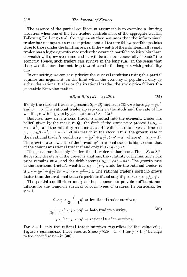
218 The Journal of Finance
The essence of the partial equilibrium argument is to examine a limitingsituation when one of the two traders controls most of the aggregate wealth.Following De Long et al. the argument then assumes that the infinitesimaltrader has no impact on market prices, and all traders follow portfolio policiesclose to those under the limiting prices. If the wealth of the infinitesimally smalltrader has a higher growth rate under the assumed portfolio policies, his shareof wealth will grow over time and he will be able to successfully “invade” theeconomy. Hence, such traders can survive in the long run, “in the sense thattheir wealth share does not drop toward zero in the long run with probabilityone.”
In our setting, we can easily derive the survival conditions using this partialequilibrium argument. In the limit when the economy is populated only byeither the rational trader or the irrational trader, the stock price follows thegeometric Brownian motion
dSt = St(μS dt + σS dBt). (29)
If only the rational trader is present, St = S∗t and from (13), we have μS = γ σ 2
and σS = σ . The rational trader invests only in the stock and the rate of hiswealth growth is given by μS − 1
2σ 2
S = 12(2γ − 1)σ 2.
Suppose, now an irrational trader is injected into the economy. Under hisbelief (given by the measure Q), the drift of the stock price process is μ̂S =μS + σ 2η and the volatility remains at σ . He will choose to invest a fractionwn = μ̂S/(γ σ 2) = 1 + η/γ of his wealth in the stock. Thus, the growth rate of
the irrational trader’s wealth is μS − 12σ 2 + 1
2σ 2
γ 2 η (γ η − η), where η = 2(γ − 1).
The growth rate of wealth of the “invading” irrational trader is higher than thatof the dominant rational trader if and only if 0 < η < γη .
Next, assume that only the irrational trader is dominant. Then, St = S∗∗t .
Repeating the steps of the previous analysis, the volatility of the limiting stockprice remains at σ , and the drift becomes μS = γ σ 2 − ησ 2. The growth rateof the irrational trader’s wealth is μS − 1
2σ 2, while for the rational trader, it
is μS − 12σ 2 + 1
2σ 2
γ 2 (2γ − 1)η(η − γ
2γ − 1η ). The rational trader’s portfolio grows
faster than the irrational trader’s portfolio if and only if η < 0 or η >γ
2γ − 1η .
The partial equilibrium analysis thus appears to provide sufficient con-ditions for the long-run survival of both types of traders. In particular, forγ > 1,
0 < η <γ
2γ − 1η ⇒ irrational trader survives,
γ
2γ − 1η < η < γη ⇒ both traders survive,
η < 0 or η > γη ⇒ rational trader survives.
(30)
For γ = 1, only the rational trader survives regardless of the value of η.Figure 8 summarizes these results. Since γ /(2γ − 1) ≤ 1 for γ ≥ 1, η belongsto the second region in (30).

The Price Impact and Survival of Irrational Traders 219
1 1.5 22
1
0
1
2sr
ed
art la
noit
arrI′
,feil
eb
η
Risk aversion, γ
N
R
R
N,R
Partial Equilibrium, Survival
Figure 8. The survival of rational and irrational traders for different values of η and γ in partial
equilibrium. For each region in the parameter space, we highlight which of the agents survives in
the long run: “R” means that survival of the rational trader is guaranteed inside the region; “N”
corresponds to the irrational trader; and “N,R” means that both traders survive.
The survival conditions given in Figure 8 clearly differ from the survivalconditions from the general equilibrium analysis shown in Figure 5. The dif-ference occurs when γ
2γ−1η < η < γη . In particular, the partial equilibrium
argument predicts survival of both traders for these parameter values, whilegeneral equilibrium analysis shows the extinction of the irrational trader whenη > η .
The difference in results from the partial equilibrium argument comes fromits two assumptions: (i) when the irrational trader becomes small in relativewealth, the stock price behaves as if he is absent, and (ii) both traders adoptthe portfolio policies that would be optimal under that limiting price process.We know from our analysis in Section IV that the first assumption is generallyfalse. But the more direct reason for the discrepancy in survival results is be-cause the second assumption is false. For instance, η < η < γη corresponds toCase 3 of Proposition 5, wherein the stock price is asymptotically the same as inthe economy without the irrational trader. In other words, the irrational traderhas no significant impact on the current stock price as his wealth becomes

220 The Journal of Finance
negligible. The moments of stock returns converge to the values implied by thepartial equilibrium analysis. However, as we show in Section VII, the irrationaltrader’s portfolio policy differs significantly from what the partial equilibriumanalysis assumes. In particular, he does not simply hold the portfolio implied bythe limiting price process. This explains the deviations in the conclusions aboutlong-run survival from the heuristic partial equilibrium argument and demon-strates the limitations of partial equilibrium arguments and the importance ofequilibrium effects on survival.
IX. Conclusion
The analysis above examines the long-run price impact and survival of irra-tional traders who use persistently wrong beliefs to make their portfolio choices.Using a parsimonious model with no intermediate consumption, we show thatirrational traders can maintain a persistent influence on prices even after theyhave lost most of their wealth. Our analysis of conditions for survival of eithertype of traders further highlights the importance of taking into account theeffect that traders have on asset prices.
For tractability, we confine our analysis to preferences with constantrelative-risk aversion. Extensions of our analysis to more general preferencesare possible and may yield unexpected results. We also assume that the rationaland irrational traders differ only in their beliefs but not in their preferences.This allows us to focus on the impact of irrational beliefs on survival and prices.Of course, differences in time and risk preferences can have their own set ofimplications for long-run survival. Perhaps more important is the extension ofthese results to models with intermediate consumption and alternative prefer-ences. While there is more to be done in this area, it is fair to say that a generalmessage is emerging and is unlikely to be overturned. Namely, survival andprice impact are related but distinct concepts and arguments ignoring sucha distinction are unreliable. In our model, irrational traders can survive andeven dominate rational traders, but even when they do not survive, they canstill have a persistent impact on asset prices.
Appendix
Proof of Proposition 1: The optimality conditions of the maximization prob-lem in (9a) require that
Cr,T = Cn,T (b ξT )1/γ . (A1)
Combined with the market clearing condition (9b), this implies (10a) and (10b).The SPD must be proportional to the traders’ marginal utilities. Since we set
the interest rate equal to zero, the SPD conditional on the information availableat time t is given by (1 + (b ξT )1/γ )γ D−γ
T /Et[(1 + (b ξT )1/γ )γ D−γ
T ]. The price of anypayoff ZT is therefore given by (12).
The individual budget constraint in a dynamically complete market is equiv-alent to the static constraint that the initial wealth of a trader is equal to the

The Price Impact and Survival of Irrational Traders 221
present value of the trader’s consumption (e.g., Cox and Huang (1989)). Sincethe two traders in our model have identical endowments at time t = 0, theirbudget constraints imply
Wr,0 = E0
[D1−γ
T
(1 + (b ξT )
1γ
)γ−1]E0
[D−γ
T
(1 + (b ξT )
1γ
)γ ] = E0
[D1−γ
T (b ξT )1γ
(1 + (b ξT )
1γ
)γ−1]E0
[D−γ
T
(1 + (b ξT )
1γ
)γ ] = Wn,0.
(A2)
We now verify that b = eησ 2(γ−1)T satisfies (A2). Note that
D1−γ
T = e[(1−γ )(μ− σ2
2)+ 1
2(1−γ )2σ 2]T e− 1
2(1−γ )2σ 2T+(1−γ )σ BT . (A3)
Define a new measure Q, such that ( d Qd P )T = e− 1
2(1−γ )2σ 2T+(1−γ )σ BT , where P is the
original probability measure. Using the translation invariance property of the
Gaussian distribution, the random variable BQT = BT − (1 − γ )σT is a standard
normal random variable under Q. Thus, the equality
E0
[D1−γ
T (b ξT )1γ
(1 + (b ξT )
1γ
)γ−1]
= E0
[D1−γ
T
(1 + (b ξT )
1γ
)γ−1]
is equivalent to
EQ0
[(ξ
QT
) 1γ(1 + (
ξQT
) 1γ)γ−1
]= E
Q0
[(1 + (
ξQT
) 1γ)γ−1
],
where ξQT = exp(− 1
2σ 2η2T + σηBQ
T ). Since the variable BQT is equivalent in dis-
tribution to BT, we can restate the last equality equivalently as
E0
[ξ
1γ
T
(1 + ξ
1γ
T
)γ−1]= E0
[(1 + ξ
1γ
T
)γ−1].
To verify that the above equality holds, consider a function F(z) defined as
F (z) = E0
[(e
12γ
zT + e− 12γ
zTξ
1γ
T
)γ ].
Changing the order of the differentiation and expectation operators (seeBillingsley (1995, Th. 16.8)),
F ′(z)|z=0 = E
[1
2
(1 − ξ
1γ
T
)(1 + ξ
1γ
T
)γ−1]
.
Thus, it suffices to prove that F ′(z)|z=0 = 0. Since
E0
[(e
12γ
zT + e− 12γ
zTξ
1γ
T
)γ ]= E0
[(e
12γ
(zT− 12η2σ 2T+ησ BT ) + e− 1
2γ(zT− 1
2η2σ 2T+ησ BT )
)γ
ξ12
T
],
if we both define a new measure Q so that ( dQdP )T = e− 1
8η2σ 2T+ 1
2ησ BT and use a
change of measure similar to its earlier application in this proof, we find that
E0
[(e
12γ
zT + e− 12γ
zTξ
1γ
T
)γ ]= E0
[(e
12γ
(zT+ησ BT ) + e− 12γ
(zT+ησ BT ))γ ]
e− 18η2σ 2T .
222 The Journal of Finance
The symmetry of the distribution of the normal random variable BT impliesthat F(z) = F(−z), and therefore F′(z)|z=0 = 0. This verifies that b = eησ 2(γ−1)T .
We now prove that the conditional volatility of stock returns isbounded between σ and σ (1 + |η|). Define A = e(−ησ 2/γ )(T−t) and g =e− 1
2η2σ 2 1
γT+σ 2η(γ−1) 1
γt+ ησ
γBT . The stock price can be expressed as
St = Et[D1−γ
T
(1 + (bξT )1/γ
)γ ]Et
[D−γ
T
(1 + (bξT )1/γ
)γ ] = e(μ−σ 2γ )T+(− 12σ 2(1−2γ ))t eσ Bt
Et[(1 + g )γ ]
Et[(1 + g A)γ ]. (A4)
By Ito’s Lemma, its volatility σSt is given by
σSt = ∂ ln St
∂ Bt= σ + ησ
(Et[(1 + g A)γ−1]
Et[(1 + g A)γ ]− Et[(1 + g )γ−1]
Et[(1 + g )γ ]
). (A5)
To establish the bounds on stock return volatility, we prove that
Et[(1 + g A)γ−1]
Et[(1 + g A)γ ]− Et[(1 + g )γ−1]
Et[(1 + g )γ ]≥ 0 (A6)
for A ≤ 1, with the opposite inequality for A ≥ 1. Note that for any twice-differentiable function F(A, γ ),
∂
∂γ
∂
∂ Aln(F (A, γ )) ≥ 0 ⇒ ∂
∂ Aln(F (A, γ − 1)) − ∂
∂ Aln[F (A, γ )] ≤ 0
⇒ ∂
∂ AF (A, γ − 1)
F (A, γ )≤ 0.
Thus, to prove (A6), it suffices to show that ∂2 ln(Et[(1+ g A)γ ])/ ∂ A∂γ ≥ 0.The function (1 + gA)γ is log-supermodular in A, g, and γ , since it is pos-itive and its cross-partial derivatives in all arguments are positive. Thus,according to the additivity property of log-supermodular functions (see, forexample, Athey (2002)), Et[(1+ g A)γ ] is log-supermodular in A and γ , that is,∂2 ln(Et[(1+ g A)γ ])/ ∂ A∂γ ≥ 0.
Because A > 1 if and only if η < 0, we have shown that
η
(Et[(1 + g A)γ−1]
Et[(1 + g A)γ ]− Et[(1 + g )γ−1]
Et[(1 + g )γ ]
)≥ 0 (A7)
and hence σSt ≥ σ .
Because ( Et [(1 + g A)γ−1]Et [(1 + g A)γ ]
− Et [(1 + g )γ−1]Et [(1 + g )γ ]
) is bounded between −1 and 0 for η < 0,
and between 0 and 1 for η > 0, we obtain the upper bound from (A5): σSt ≤σ (1 + |η|). Q.E.D.
Proof of Proposition 3: We will make use of the following result:
LEMMA A1: Let N(x) denote the cumulative density function of the standardnormal distribution: N (x) ≡ 1√
2π
∫ ∞x e− z2
2 dz. For x > 0, N (x) ≤ 12e− x2
2 .

The Price Impact and Survival of Irrational Traders 223
Proof of Lemma A1: N (x) = 1√2π
∫ ∞x e− z2
2 dz ≤ 1√2π
∫ ∞x e− x2
2− (z−x)2
2 dz = 12e− x2
2 .
Note that for convenience, we define the cumulative density function as theprobability above a given value rather than below. Q.E.D.
Let t = T/(1 + |η|) and define M =√
2−12
σ |η|t. According to Lemma A1,
Prob[|Bt | ≥ M√
t]] = 2 N (M√
t) ≤ e− M2
2t = e− (
√2−1)2
2σ 2η2t ≤ e− 1
12σ 2η2t .
On the set {|Bt | ≤ M√
t},
αn,t = ξt
1 + ξt≤ ξt ≤ e− σ2η2
2t+σ |η|Mt = e− 3−2
√2
2σ 2η2t ≤ e− 1
12σ 2η2t ≤ ε.
Therefore,
Prob[αn,t ≥ ε] ≤ Prob[|Bt | ≥ M√
t] ≤ e− 112
σ 2η2t ≤ ε, (A8)
which establishes the first result of the proposition. The second result followsfrom the fact that on the set {|Bt | ≤ M
√t},
St
S∗t
≤ e−σ 2|η|(T−t) 1
αn,t≤ e−σ 2|η|(T−t)+ σ2η2
2t+σ |η|M√
t ≤ e− σ2η2
2t+σ |η|Mte−σ 2|η|T+σ 2|η|(1+|η|)t .
Given that on the set {|Bt | ≤ M√
t}, e− σ2η2
2t+σ |η|Mt ≤ e− 1
12σ 2η2t , and since
t = T/(1 + |η|), e−σ 2|η|T+σ 2|η|(1+|η|)t ≤ 1. We conclude that on the set {|Bt | ≤M
√t}, St
S∗t
≤ e− 112
σ 2η2t and hence
Prob
[1 − St
S∗t
≤ 1 − ε
]≤ e− 1
12σ 2η2t ≤ ε, (A9)
which concludes the proof of the proposition. Q.E.D.
Proof of Proposition 4: According to (10a) and (10b),
Cn,T
Cr,T= (b ξT )1/γ = exp
[1
γ
(−1
2σ 2η2 + ησ 2(γ − 1)
)T + 1
γησ BT
]. (A10)
Using the strong Law of Large Numbers for Brownian motion (see Karatzasand Shreve (1991, Sec. 2.9.A)), for any value of σ ,
limT→∞
ea T+σ BT ={
0, a < 0∞, a > 0,
where convergence takes place almost surely. The proposition then follows.Q.E.D.
Proof of Proposition 5: Our analysis will make use of the following technicalresult.
LEMMA A2: Consider a stochastic process X t = ec t+v Bt and a constant a ≥ 0.Assume that ac + 1
2v2a2(1 − λ) �= 0, 0 ≤ λ < 1. Then the limit limT→∞Et[Xa
T] is

224 The Journal of Finance
equal to either zero or infinity almost surely, where we set t = λT. The followingconvergence results hold:
(i) (Point-wise convergence)
limT→∞
Et[(1 + X T )a
]1 + Et
[X a
T
] = 1. (A11)
(ii) (Convergence of moments)
limT→∞
meant Et[(1 + X T )a
]meant
(1 + Et
[X a
T
]) = 1, limT→∞
volt Et[(1 + X T )a
]volt
(1 + Et
[X a
T
]) = 1, (A12)
where meantft and voltft denote the instantaneous mean and standard deviationof the process ln ft, respectively.
Proof of Lemma A2: (i) Consider the conditional expectation
Et[X a
T
] = exp
[ac T + 1
2v2a2(1 − λ) T + avBt
]. (A13)
The limit of Et[XaT] is equal to zero if ac + 1
2v2a2(1 − λ) < 0 and equal to infinity
if the opposite inequality holds (according to the strong Law of Large Numbersfor Brownian motion; see Karatzas and Shreve (1991, Sec. 2.9.A)).
Because the function ac T + 12v2a2(1 − λ) T is convex in a and equal to zero
when a = 0, we find that for a ≥ 1,
Et[X a
T
] → ∞ ⇒ Et[X z
T
]Et
[X a
T
] → 0, ∀z ∈ (0, a) (A14a)
Et[X a
T
] → 0 ⇒ Et[X z
T
] → 0, ∀z ∈ (0, a). (A14b)
We prove the result of the Lemma separately for six regions covering theentire parameter space.
Case 1: 0 ≤ a ≤ 1, Et[XaT] → ∞. If XT ≤ 1, (XT + 1)a ≤ 2a, whereas if XT ≥
1, (XT + 1)a − XaT ≤ aXa−1
T ≤ a since (XT + 1)a is concave and a − 1 ≤ 0. There-fore, Xa
T ≤ (1 + XT)a ≤ XaT + 2a + a and, hence, limT→∞Et[(1 + XT)a]/Et[Xa
T] = 1,which implies limT→∞Et[(1 + XT)a]/(1 + Et[Xa
T]) = 1.
Case 2: 1 ≤ a ≤ 2, Et[XaT] → ∞. By the mean value theorem, (1 + XT)a =
XaT + a(w + XT)a−1 for some w ∈ [0, 1]. Using the analysis of Case 1, (w +
XT)a−1 ≤ (1 + XT)a−1 ≤ Xa−1T + 2a−1 + a − 1, which combined with (A14a), im-
plies that limT→∞ Et[(1 + X T )a]/Et[X a
T
] = 1 and the main result follows.
Case 3: 2 ≤ a, Et[X aT ] → ∞. By the mean value theorem, (1 + XT)a = Xa
T +a(w + XT)a−1 for some w ∈ [0, 1]. By Jensen’s inequality, [(1 + XT)/2]a−1 ≤ (1 +Xa−1
T )/2. Thus, 0 ≤ (w + XT)a−1 ≤ (1 + XT)a−1 ≤ 2a−2 + 2a−2Xa−1T , which com-
bined with (A14a), implies that limT→∞Et[(1 + XT)a]/Et[XaT] = 1 and the main
result follows.

The Price Impact and Survival of Irrational Traders 225
Case 4: 0 ≤ a ≤ 1, Et[X aT ] → 0: If XT ≤ 1, (1 + XT)a ≤ 1 + XT ≤ 1 + Xa
T, whileif XT ≥ 1, (1 + XT)a ≤ Xa
T + a ≤ 1 + XaT since (1 + XT)a is concave. Thus, 1 ≤
(1 + XT)a ≤ 1 + XaT and, therefore, limT→∞ Et[(1 + X T )a] = 1, which implies the
main result.
Case 5: 1 ≤ a ≤ 2, Et[X aT ] → 0. By the mean value theorem, (1 + XT)a = 1 +
aXT(1 + wXT)a−1 for some w ∈ [0, 1]. Furthermore, XT(1 + wXT)a−1 ≤ XT(1 +XT)a−1 ≤ XT(Xa−1
T + 2a−1 + a − 1), using the same argument as in Case 1.Since limT→∞Et[Xa
T] = 0, according to (A14b), limT→∞Et[XT] = 0 and hencelimT→∞ Et[(1 + X T )a] = 1.
Case 6: 2 ≤ a, Et[X aT ] → 0. By the mean value theorem, (1 + XT)a = 1 +
aXT(1 + wXT)a−1 for some w ∈ [0, 1]. Furthermore, XT(1 + wXT)a−1 ≤ XT(1 +XT)a−1 ≤ 2a−2XT + 2a−2Xa
T by Jensen’s inequality. Since limT→∞Et[XaT] = 0 ac-
cording to (A14b), and limT→∞Et[XT] = 0, then limT→∞ Et[(1 + X T )a] = 1.
(ii) Since the conditional expectations Et[(1 + XT)a] and Et[1 + XaT] are mar-
tingales, they have zero drift for all values of T and t. By Ito’s Lemma, con-vergence of the first moments of the natural logarithms of the same processesfollows from convergence of the second moments.
We now establish convergence of volatility of the process Et[(1 + XT)a].According to Ito’s Lemma, one must show that
limT→∞
∂ ln Et[(1 + X T )a
] /∂ Bt
∂ ln(1 + Et
[X a
T
])/∂ Bt
= 1, ∀ a ≥ 0.
Given (A13), it suffices to prove that limT→∞ ∂ ln Et[(1 + X T )a]/∂ Bt = 0if limT→∞Et[Xa
T] = 0, and limT→∞∂ln Et[(1 + XT)a]/∂Bt = av if limT→∞Et[XaT]
= ∞.First, changing the order of differentiation and expectation operators (see
Billingsley (1995, Th. 16.8)),
∂ ln Et[(1 + X T )a
]∂ Bt
= avEt
[X T (1 + X T )a−1
]Et
[(1 + X T )a
] = av
(1 − Et
[(1 + X T )a−1
]Et
[(1 + X T )a
] ).
Furthermore, according to part (i),
Et[(1 + X T )a−1
]Et
[(1 + X T )a
] ∼ Et[(1 + X T )a−1
]1 + Et
[X a
T
] . (A15)
Assume a ≥ 1. As we show in Case 1 of the Proof of part (i), Xa−1T ≤ (1 + XT)a−1 ≤
Xa−1T + 2a−1 + a − 1. If Et[X a
T ] → ∞, according to (A14a), Et[X a−1T ]/Et[X a
T ] →0, which yields limT→∞∂ln Et[(1 + XT)a]/∂Bt = av. Similarly, if Et[X a
T ] → 0,
then, according to (A14b), limT→∞Et[Xa−1T ] = 0, which according to part (i) im-
plies that limT→∞Et[(1 + XT)a−1] = 1 and limT→∞∂ln Et[(1 + XT)a]/∂Bt = 0.Next, consider the case of 0 < a < 1. If Et[X a
T ] → ∞, because Et[(1 +X T )a−1] ≤ 1, (A15) implies limT→∞∂ln Et[(1 + XT)a]/∂Bt = a v.
Suppose limT→∞ Et[X aT ] = 0. By Markov’s inequality, for any ε > 0, Pt[XT >
ε] ≤ Et[XaT]/εa → 0. Similarly, Pt[XT < ε] ≤ Et[(1 + XT)a−1]/(1 + ε)a−1. Thus,

226 The Journal of Finance
1 ≥ Et[(1 + XT)a−1] ≥ Pt[XT < ε](1 + ε)a−1, and lim infT→∞Et[(1 + XT)a−1] ≥(1 + ε)a−1 for any ε > 0. This implies that limT→∞Et[(1 + XT)a−1] = 1 andlimT→∞∂ln Et[(1 + XT)a]/∂Bt = 0. Q.E.D.
We establish the long-run behavior of St for the case γ > 1 and 0 < η < η =2(γ − 1). The results for all other regions in the parameter space can be obtainedsimilarly.
The equilibrium stock price and the ratio of the individual wealth processesare given by
St =Et
[D1−γ
T
(1 + (b ξT )
1γ
)γ]
Et
[D−γ
T
(1 + (b ξT )
1γ
)γ] ,
Wr,t
Wn,t=
Et
[D1−γ
T
(1 + (b ξT )
1γ
)γ−1]
Et
[D1−γ
T (b ξT )1γ (1 + (b ξT )
1γ
)γ−1] . (A16)
We therefore need to characterize the long-run behavior of the following twoquantities:
E (1) ≡ Et
[D1−γ
T (1 + (b ξT )1γ
)γ], E (2) ≡ Et
[D−γ
T
(1 + (b ξT )
1γ
)γ]. (A17)
Consider the first expression,
E (1) = Et
[D1−γ
T
(1 + (b ξT )
1γ
)γ]
= D1−γt Et
[(DT
Dt
)1−γ(
1 +(
b ξtξT
ξt
) 1γ
)γ ]. (A18)
Given the aggregate dividend process,(DT
Dt
)1−γ
= e(T−t)(μ(1−γ )− 12σ 2(1−γ )γ )e− 1
2(1−γ )2σ 2(T−t)+(1−γ )σ (BT −Bt ).
As in the Proof of Proposition 1, we introduce a new measure Q with the
Radon–Nikodym derivative ( d Qd P )t = e− 1
2(1−γ )2σ 2(T−t)+(1−γ )σ (BT −Bt ). By Girsanov’s
theorem, BT − Bt = BQT − BQ
t − (1 − γ )σ (T − t), where BQt is a Brownian mo-
tion under the measure Q. Using the expression for b from Proposition 1,b = eT (γ−1)σ 2η, we find
E (1) = eT (μ(1−γ )− 12σ 2(1−γ )γ )+t(− 1
2σ 2(1−γ )2)+Bt (σ (1−γ ))
× EQt
[(1 + e(− 1
2η2σ 2 1
γ)T+( 1
γ(γ−1)σ 2η)t+ ησ
γBQ
T
)γ ].
We omit the superscript Q, since the distribution of BQt under the measure Q
is the same as the distribution of Bt under the original measure P.Using the assumption that t = λT, define
X T = e(− 12η2σ 2 1
γ+(1−λ) 1
γ(γ−1)σ 2η)T+ ησ
γBT . (A19)
We now apply the result of Lemma A2, with
c = −1
2η2σ 2 1
γ+ (1 − λ)
1
γ(γ − 1)σ 2η, v = ησ
γ, a = γ.

The Price Impact and Survival of Irrational Traders 227
Since we assume γ > 1 and 0 < η < 2(γ − 1), limT→∞Et[XaT] = ∞. According to
Lemma A2,
Et
[D1−γ
T
(1 + (b ξT )
1γ
)γ]
∼ e(μ(1−γ )− 12σ 2(1−γ )γ )T+(− 1
2σ 2(η+1−γ )2)t+σ (η+1−γ )Bt .
We next examine E(2). Using a similar change of measure, we find
E (2) = e(−μγ+ 12σ 2(1+γ )γ )T+(− 1
2σ 2γ 2)t+(−σγ )Bt
× Et[(
1 + e(−σ 2η 1γ− 1
2η2σ 2 1
γ)T+σ 2ηt+ ησ
γBT
)γ ]. (A20)
We apply Lemma A2, setting X T = ec T+v BT and
c = −σ 2η1
γ− 1
2η2σ 2 1
γ+ (1 − λ)σ 2η, v = ησ
γ, a = γ.
The value of limT→∞Et[XaT] depends on the exact combination of the model
parameters. In particular,
limT→∞
Et[X a
T
] ={
∞, −2η + λ(2γ η − η2) > 0,
0, −2η + λ(2γ η − η2) < 0,
(see the Proof of Lemma A2, part (i)). Define λS ≡ 22γ−η
. Note that because γ > 1
and 0 < η < 2(γ − 1), 0 < λS < 1. Then, limT→∞Et[XaT] = ∞ if λ > λS and 2γ η −
η2 > 0 or if λ < λS and 2γ η − η2 < 0, and the limit is equal to zero otherwise.By Lemma A2, if limT→∞Et[Xa
T] = ∞,
Et
[D−γ
T (1 + (b ξT )1γ )γ
]∼ eT (−μγ+ 1
2σ 2(1+γ )γ−σ 2η)T+(− 1
2σ 2(η−γ )2)t+σ (η−γ )Bt ,
while if limT→∞Et[XaT] = 0, then
Et
[D−γ
T (1 + (b ξT )1γ )γ
]∼ e(−μγ+ 1
2σ 2(1+γ )γ )T+(− 1
2σ 2γ 2)t+(−σγ )Bt .
Using our definition of λS, we re-state these results as
Et
[D−γ
T
(1 + (b ξT )
1γ
)γ]
∼{
e(−μγ+ 12σ 2(1+γ )γ )T+(− 1
2σ 2γ 2)t−σγ Bt , 0 ≤ λ < λS
e(−μγ+ 12σ 2(1+γ )γ−σ 2η)T+(− 1
2σ 2(η−γ )2)t+σ (η−γ )Bt , λS < λ ≤ 1.
Having established the behavior of both the numerator and the denominatorof the expression for the stock price, we have proven the limiting result for thestock price itself. According to part (ii) of Lemma A2, not only the stock price,but also the mean and volatility of returns behave according to the asymp-totic expressions of Proposition 5 in the limit of the economy with horizon Tapproaching infinity. Q.E.D.
228 The Journal of Finance
Proof of Proposition 7: When the financial markets are dynamically completeand there is a single source of uncertainty (driven by a Brownian motion), thefraction of the agent’s wealth invested in stock can be computed as a ratio of theinstantaneous volatility of the agent’s wealth to the instantaneous volatility ofthe cumulative stock return process. Proposition 5 (and Kogan et al. (2003),Proposition 8) provide the expression for the long-run behavior of the volatilityof stock returns and individual wealth processes, from which the expression forportfolio holdings follows immediately. To decompose the portfolio holdings ofthe rational trader into a sum of the myopic and hedging demands, we computethe hedging demand as μS/(γ σ 2
S ), where μS and σS are the drift and the diffusioncoefficients of the stock return process, respectively. The difference between thetotal portfolio holdings and the myopic component define the agent’s hedgingdemand. For the irrational trader, the calculations are analogous, except themyopic demand is given by (μ̂S/(γ σ 2
S) = (μS + ησσS)/(γ σ 2S)), where μ̂S is the
expected stock return as perceived by the irrational trader. Q.E.D.
REFERENCESAlpert, Marc, and Howard Raiffa, 1982, A progress report on the training of probability assessors,
in D. Kahneman, P. Slovic, and A. Tversky eds.: Judgement Under Uncertainty: Heuristics andBiases (Cambridge University Press, Cambridge, U.K.).
Athey, Susan, 2002, Monotone comparative statics under uncertainty, Quarterly Journal of Eco-nomics 117, 187–223.
Benartzi, Shlomo and Richard H. Thaler, 2001, Naive diversification strategies in defined contri-
bution saving plans, American Economic Review 91, 79–98.
Billingsley, Patrick, 1995, Probability and Measure, 3rd ed. (Wiley-Interscience, New York).
Black, Fischer, 1986, Noise, Journal of Finance 41, 529–543.
Black, Fischer, and Myron S. Scholes, 1973, The pricing of options and corporate liabilities, Journalof Political Economy 81, 637–654.
Blume, Lawrence, and David Easley, 2001, If you’re so smart, why aren’t you rich? Belief selection
in complete and incomplete markets, Cowles Foundation Discussion Papers, 1319.
Cox, John, and Chi-fu Huang, 1989, Optimal consumption and portfolio policies when asset prices
follow a diffusion process, Journal of Economic Theory 49, 33–83.
De Long J., Bradford Andrei Shleifer, Lawrence H. Summers, and Robert J. Waldman, 1991, The
survival of noise traders in financial markets, Journal of Business 64, 1–19.
Duffie, Darrell, and Chi-fu Huang, 1985, Implementing Arrow–Debreu equilibria by continuous
trading of few long-lived securities, Econometrica 53, 1337–1356.
Figlewski, Stephen, 1978, Market “efficiency” in a market with heterogeneous information, Journalof Political Economy 86, 581–597.
Friedman, Milton, 1953, The case for flexible exchange rates, in Essays in Positive Economics(University of Chicago Press, Chicago).
Hakansson, Nils H., 1971, Capital growth and the mean-variance approach to portfolio selection,
Journal of Financial and Quantitative Analysis 6, 517–557.
Harrison, J. Michael, and David M. Kreps, 1979, Martingales and arbitrage in multiperiod securi-
ties markets, Journal of Economic Theory 2, 381–408.
Kahneman, Daniel, and Amos Tversky, 1979, Prospect theory: An analysis of decision under risk,
Econometrica 47, 263–291.
Karatzas, Ioannis, and Steven E. Shreve, 1991, Brownian Motion and Stochastic Calculus, 2nd ed.
(Springer-Verlag, New York).
Kogan, Leonid, Stephen A. Ross, Jiang Wang, and Mark M. Westerfield, 2003, The survival and
price impact of irrational traders, NBER Working paper 9434.

The Price Impact and Survival of Irrational Traders 229
Lucas, Robert E., Jr., 1978, Asset prices in an exchange economy, Econometrica 46, 1429–
1445.
Odean, Terrance, 1998, Are investors reluctant to realize their losses? Journal of Finance 53, 1775–
1798.
Radner, Roy, 1972, Existence of equilibrium of plans, prices, and price expectations in a sequence
of markets, Econometrica 40, 289–303.
Sandroni, Alvaro, 2000, Do markets favor agents able to make accurate predictions? Econometrica68, 1303–1341.
Wang, Jiang, 1996, The term structure of interest rates in a pure exchange economy with hetero-
geneous investors, Journal of Financial Economics 41, 75–110.