Self-Identity and Brand Choice: A Brand Relationship Perspective
Upload
andrew-chingCategory
view
215download
0
JOURNAL OF APPLIED ECONOMETRICSJ. Appl. Econ. 24: 393–420 (2009)Published online in Wiley InterScience(www.interscience.wiley.com) DOI: 10.1002/jae.1053
THE PRICE CONSIDERATION MODEL OF BRAND CHOICE
ANDREW CHING,a TULIN ERDEM,b AND MICHAEL KEANEc,d*a Rotman School of Management, University of Toronto, Canada
b Stern School of Business, New York University, USAc ARC Federation Fellow, University of Technology, Sydney
d Research Professor, Arizona State University, USA
SUMMARYThe workhorse brand choice models in marketing are the multinomial logit (MNL) and nested multinomiallogit (NMNL). These models place strong restrictions on how brand share and purchase incidence priceelasticities are related. In this paper, we propose a new model of brand choice, the “price consideration”(PC) model, that allows more flexibility in this relationship. In the PC model, consumers do not observeprices in each period. Every week, a consumer decides whether to consider a category. Only then does he/shelook at prices and decide whether and what to buy. Using scanner data, we show the PC model fits muchbetter than MNL or NMNL. Simulations reveal the reason: the PC model provides a vastly superior fit tointer-purchase spells. Copyright 2009 John Wiley & Sons, Ltd.
1. INTRODUCTION
The workhorse brand choice model in quantitative marketing is unquestionably the multinomiallogit (MNL). It is often augmented to include a no-purchase option. Occasionally, nestedmultinomial logit (NMNL) or multinomial probit (MNP) models are used to allow for correlationsamong the unobserved attributes of the choice alternatives, or the models are extended to allowfor consumer taste heterogeneity. There have been rather strong arguments among proponents ofdifferent variants of these models.
But in two fundamental ways, all these workhorse brand choice models are more alike thandifferent: (1) they assume essentially static behavior on the part of consumers, in the sense thatchoices are based only on current (and perhaps past) but not expected future prices, and (2) theyall make strong (albeit different) assumptions about when consumers see prices, and when theyconsider purchasing in a category.
For instance, any brand choice model that does not contain a no-purchase option is a purchasetiming/incidence model—of a very strong form. This incidence model says that a random andexogenous process1 determines when a consumer decides to buy in a category, and that theconsumer only sees prices after he/she has already decided to buy. On the other hand, standardbrand choice models that contain a no-purchase option make an opposite and equally strongassumption: that consumers see prices in every week,2 and decide whether to purchase in the
Ł Correspondence to: Michael Keane, School of Finance and Economics, University of Technology Sydney, P.O. Box 123Broadway, NSW 2007, Australia. E-mail: [email protected] By “exogenous” we mean unrelated to prices, promotion, tastes and inventories.2 For expositional convenience, throughout the paper we will treat the week as the decision period.
Copyright 2009 John Wiley & Sons, Ltd.
394 A. CHING, T. ERDEM AND M. KEANE
category based on these weekly price vectors.3 And, in either case, whether one assumes consumerssee prices always or only if they have already decided to buy, standard models assume thatconsumers then make decisions solely based on current (and perhaps past) prices.
In this paper we propose a fundamentally different model of brand choice that we call the “priceconsideration” or PC model. The difference between this and earlier brand choice models is that,in the PC model, consumers make a weekly decision about whether to consider a category, andthis decision is made prior to seeing any price information. Of course, the decision will dependon inventory, whether the brand is promoted in the media, and so on. Only after the consumerhas decided to consider a category does he/she see prices. In this second stage, the consumerdecides whether and what brand to buy. Thus, the PC model provides a middle ground betweenthe extreme price awareness assumptions that underlie conventional choice models (i.e., alwaysvs. only when you buy) because in the PC model consumers see prices probabilistically.
We estimate the PC model on Nielsen scanner data for the ketchup and peanut butter categories.We compare the fit of the PC model to both MNL with a no-purchase option, and NMNL withthe category purchase decision at the upper level of the nest. All three models incorporate (i) statedependence in brand preferences a la Guadagni and Little (1983), (ii) dependence of the valueof no-purchase on duration since last purchase (to capture inventory effects), and (iii) unobservedheterogeneity in brand intercepts.4
We find that the PC model produces substantially superior likelihood values to both the MNL andNMNL, and dominates on the AIC and BIC criteria. Simulation of data from the models revealsthat the PC model produces a dramatically better fit to observed inter-purchase spell lengths thando the MNL and NMNL models. In particular, the conventional models greatly exaggerate theprobability of short spells. For the PC model, this problem is much less severe.
To our knowledge, this severe failure of conventional MNL and NMNL choice models to fit spelldistributions has not been previously noted—or, even if it has, it is certainly not widely known.We suspect this is because it is common in the marketing literature to evaluate models basedon in-sample and holdout likelihoods, and fit to choice frequencies, while fit to choice dynamicsis rarely examined. Since the PC model is as easy to estimate as the conventional models,5 weconclude it should be viewed as a serious alternative to MNL and NMNL.
2. PROBLEMS WITH CONVENTIONAL CHOICE MODELS, AND THE PC ALTERNATIVE
Keane (1997a) argued that conventional MNL and NMNL choice models (with or without no-purchase) could produce severely biased estimates of own and cross-price elasticities of demand,if inventory-planning behavior by consumers is important. To understand his argument, considerthis simple example. Say there are two brands, A and B, and that consumers are totally loyal toeither one or the other. The following table lists the number of consumers who buy A, B or makeno-purchase over a 5 week span under two scenarios. First, a no promotion environment:
3 This is also true in a nested logit model, where at the top level consumers decide whether to buy in the category, and inthe lower level choose amongst brands. In such a model, the category purchase decision is based on the inclusive valuefrom the lower level of the nest, which is in turn a function of that week’s price vector.4 We assume a multivariate normal distribution of brand intercepts, so in fact we are estimating what are known as“heterogeneous logit” models (see, e.g., Harris and Keane, 1999).5 In fact, the PC model may be easier to estimate than the NMNL, as the latter often has a poorly behaved likelihood.
Copyright 2009 John Wiley & Sons, Ltd. J. Appl. Econ. 24: 393–420 (2009)DOI: 10.1002/jae
THE PRICE CONSIDERATION MODEL OF BRAND CHOICE 395
Week 1 2 3 4 5
A 10 10 10 10 10B 10 10 10 10 10No-purchase 80 80 80 80 80
And second a scenario where Brand A is on promotion (say a 20% price cut) in week 2:
Week 1 2 3 4 5
A 10 20 5 5 10B 10 10 10 10 10No-purchase 80 70 85 85 80
Now, notice that brand A’s market share goes from 50% to 67% in week 2. Brand B’s marketshare drops to 33%, even though no consumer switches away from B. Thus, a brand choicemodel without a no-purchase option would conclude that the cross-price elasticity of demand issubstantial (i.e., 34/.20 D 1.7), even though it is, in reality, zero.6
Interestingly, including a no-purchase option does not solve the basic problem. Notice thereis a post-promotion dip, presumably arising from inventory behavior, that causes the number ofpeople who buy A to drop by 50% in weeks 3 and 4, before returning to normal in week 5. Ifwe took data from the whole 5-week period, we would see that Brand A’s average sales whenat its “regular” price are 7.5, increasing to 20.0 when it is on promotion. Thus, a conventionalstatic choice model with a no purchase option would conclude the price elasticity of demand is�20.0/7.5 � 1�/�.20� D 8.3. The correct answer is that the short run elasticity is 5 and that thelong run elasticity is zero, since all the extra sales come at the expense of future sales.
As Keane (1997a) notes, the exaggeration of the elasticity could be even greater if consumers areable to anticipate future sales. For example, suppose a retailer always puts brand A on sale in week2 of every 5 week period. As consumers become aware of the pattern, they could concentrate theirpurchases in week 2, even if their price elasticity of demand were modest. Conventional choicemodels, however, would infer an enormous elasticity, since a modest 20% price cut causes salesto jump greatly in week two.
6 Erdem et al. (2003) describe the problem more formally as “dynamic selection bias.” Suppose there are several typesof consumers, each with a strong preference for one brand. Suppose further that consumers engage in optimal planningbehavior. Each period, a consumer considers his/her level of inventories and the vector of brand prices, and decides if it’sa good time to buy. In this framework, if brand A has a price cut in week t, consumers who buy in week t will contain anoverrepresentation of the type that prefers A. Thus, in the self-selected subset of consumers who buy in the category inany given week, there is a negative correlation between brand prices and brand preference (i.e., in weeks when price ofa brand is low, the sample contains an over-representation of the type of consumers who prefer that brand). This causesthe price elasticity of demand to be exaggerated.
Interestingly, this negative correlation between brand prices and brand preference induced by inventory behavior isopposite in sign to the positive correlation that has been the concern of the literature on “endogenous prices.” Thatliterature, stemming from Berry et al. (1995), deals with a fundamentally different type of data, where prices and sales areaggregated over long periods of time - in contrast to the high frequency (i.e., daily) price variation observed in scannerdata. Then, brands with high unobserved quality will tend to be high priced, inducing a positive correlation between brandprices and preferences. This biases price elasticities of demand towards zero. In scanner data, this problem of unobservedbrand quality can be dealt with simply by including brand intercepts.
Copyright 2009 John Wiley & Sons, Ltd. J. Appl. Econ. 24: 393–420 (2009)DOI: 10.1002/jae
396 A. CHING, T. ERDEM AND M. KEANE
An important paper by Sun et al. (2003) shows that the problems with conventional choicemodels noted by Keane (1997a) are not merely academic. They conduct two experiments. First,they simulate data from a calibrated model where the hypothetical consumers engage in inventory-planning behavior. Thus, Sun et al. know (up to simulation noise) the true demand elasticities.They estimate a set of conventional choice models on this data; i.e., MNL with and without no-purchase, NMNL with no-purchase. Each model includes consumer taste heterogeneity and statedependence. The MNL without no-purchase exaggerates cross-price elasticities by about 100%,while MNL and NMNL with no-purchase do so by about 50%. A dynamic structural modelof inventory-planning behavior fit to the same data produces accurate elasticity estimates—asexpected since it is the “true” model that was used to simulate the data.
Second, Sun et al. estimate the same set of models on Nielsen scanner data for ketchup.Strikingly, they obtain the same pattern. Estimated cross-price elasticities from the MNL andNMNL models that include no-purchase are about 50% greater than those implied by the dynamicstructural model that accounts for inventory-planning behavior. And those from the MNL withoutno-purchase are about 100% greater.
Thus, marketing research needs to confront the fact that own and cross-price elasticities ofdemand are much greater when estimated from pure brand choice models than from models thatinclude a no purchase option. What accounts for this phenomenon? As we’ve seen, one explanationis the inventory-planning behavior that Keane (1997a) predicted would cause such a problem.7 Inresponse, several authors, such as Erdem et al. (2003), Sun et al. (2003) and Hendel and Nevo(2004), have proposed abandoning conventional static choice models (i.e., MNL and NMNL) infavor of dynamic structural inventory-planning models. Of course, the difficultly with these modelsis that they are extremely difficult to estimate.
In this paper, we adopt a different course of action. We seek to develop a simple model—nomore complex than MNL or NMNL—that does not suffer from the problems noted by Keane(1997) and Sun et al. (2003). The motivation for our approach is two fold: First, we conjecturethat a brand choice model with a more flexible representation for category consideration/purchaseincidence may provide a more accurate reduced form approximation to consumer’s purchasedecision rules than the conventional models like MNL and NMNL. Second, we note there is asimpler way (than estimation of complex dynamic inventory models) to reconcile the pattern ofelasticities across models noted by Sun et al. (2003). The idea is simply that consumers do notchoose to observe brand prices in each period.
More specifically, we propose a two-stage “price consideration” (PC) model in which a consumerdecides, in each period, whether to consider buying in a category. This decision may be influencedby inventories, advertising, feature and display conditions. If a consumer decides to consider acategory, he/she looks at prices and decides whether and what brand to buy.8 Such a model can
7 Another potential explanation is that brands are viewed as very close substitutes. That would explain why, conditionalon purchase in a category, consumers’ choice among competing brands appears to be much more sensitive to price thantheir decision to purchase in the first place. But a well-known fact about consumer behavior is that in many frequentlypurchased product categories brand loyalty is high (i.e., rates of brand switching are low), implying that brands are notviewed as close substitutes.8 This two-stage decision process may be (an approximation to) optimal behavior in a version of an inventory-planningmodel where there is some fixed cost of examining prices, and it is only optimal to examine prices if inventories fall belowsome critical level, or if consumers observe some advertising/display/feature signal that reduces the cost of observingprices or conveys a signal that prices are likely to be low.
Alternatively, the PC model may also be viewed as departing from the optimal backward induction process (from thewhole vector of prices back to the expected utility of buying in the category) that consumers are assumed to follow in
Copyright 2009 John Wiley & Sons, Ltd. J. Appl. Econ. 24: 393–420 (2009)DOI: 10.1002/jae
THE PRICE CONSIDERATION MODEL OF BRAND CHOICE 397
generate a pattern where consumers are more sensitive to prices when choosing among brandsthan when deciding whether to buy in a category. The positive probability that consumers do noteven consider the category (i.e., they do not even see prices) creates a wedge between the brandchoice price elasticity and the purchase incidence price elasticity.
While this model is extremely simple, it has not, as far as we know, been used before in themarketing literature. It is important to note that the PC model is quite different from a nestedmultinomial logit (NMNL) model, where consumers first decide whether to buy in a category andthen, in a second stage, decide which brand to buy. In the first stage of the NMNL, the decisionwhether to purchase in the category is a function of the inclusive value from the second stage,which is, in fact, a price index for the category. Thus, the NMNL model assumes that consumerssee all prices in all periods. The second stage is different as well, because in our model thesecond stage includes a no purchase option. That is, if a consumer decides to consider a category,he/she may still decide, upon seeing prices, to choose no-purchase. A NMNL model can certainlygenerate a pattern that brand choice price elasticities substantially exceed purchase incidence priceelasticities, but it would do so by assuming that brands are very similar. As noted above, such anassumption is inconsistent with data on brand switching behavior.
There are a number of ways we can test our model against alternative models in the literature.First, we can simply ask whether it fits better than simple MNL and NMNL models that include ano purchase option. Second, our model can be distinguished from the alternative dynamic inventorystory for the same phenomenon by looking at categories where inventories are not important. Ifbrand choice price elasticities exceed purchase incidence price elasticities even for non-storablegoods, it favors the simple story.
3. THE PRICE CONSIDERATION (PC) MODEL
3.1. Basic Structure and Properties of the PC model, and Comparison to MNL and NMNL
The simplest version of the PC model takes the following form: Consider a category with Jbrands. In each time period t, prior to seeing prices, a consumer decides whether to considerthe category. Let PCt denote the probability the consumer considers the category in week t. Ifthe consumer decides to consider the category, then he/she looks at prices, and a MNL modelwith a no-purchase option governs choice behavior. Let Ujt D ˛j � ˇpjt C ejt denote utility ofpurchasing brand j at time t, where ejt is an extreme value error. Then, letting Pt�jjC� denote theprobability, conditional on considering the category, that the consumer chooses brand j at time t,we have:
Pt�jjC� D exp�˛j � ˇpjt�
1 CJ∑kD1
exp�˛k � ˇpkt�
j D 1, . . . J. �1�
“rational” choice models. In PC, consumers use a forward looking heuristic (that does not depend on prices) to decidewhether to consider a category, but then, once they do decide to consider, they engage in fully rational calculations tomake the brand choice/category purchase decision.
Copyright 2009 John Wiley & Sons, Ltd. J. Appl. Econ. 24: 393–420 (2009)DOI: 10.1002/jae
398 A. CHING, T. ERDEM AND M. KEANE
Let option JC 1 be no-purchase. Normalizing the deterministic part of its utility to zero, we have:
Pt�JC 1jC� D[
1 CJ∑kD1
exp�˛k � ˇpkt�
]�1
. �2�
Then, the unconditional probability that the consumer buys brand j at time t is:
Pt�j� D PCtPt�jjC�, �3�
and the unconditional probability of no purchase is:
Pt�JC 1� D PCtPt�JC 1jC�C �1 � PCt�. �4�
The derivative of the log odds ratio between brands j and k with respect to price of j is simply:
∂ ln[Pt�j�
Pt�k�
]∂pjt
D �ˇ, �5�
which is identical to what one obtains in the MNL model, because the PCt cancel out. However,the derivative of the log odds ratio between brand j and the no purchase option JC 1 is:
∂ ln[
Pt�j�
Pt�JC 1�
]∂pjt
D �ˇ C ˇ Ð �1 � PCt� exp�˛j � ˇpjt�
1 C �1 � PCt�J∑kD1
exp�˛k � ˇpkt�
. �6�
This expression lies in the interval (�ˇ, 0), approaching �ˇ as PCt " 1. Thus, if PCt < 1, our modelimplies a greater price elasticity of the brand choice log odds than that for purchase incidence.
Comparison of (5) and (6) reveals the intuition for identification of PCt in our model. (5) impliesthat the independence of irrelevant alternatives (IIA) property holds among brands, but (6) showsthat it does not hold between brands and the no purchase option. Thus, this type of departure fromIIA can be explained by our model with PCt < 1, but not by a standard MNL model with a nopurchase option. Thus, the PC model is more flexible than the MNL in terms of how price canaffect purchase incidence vs. choice amongst brands.
Next, we examine how price elasticities for purchase incidence vs. brand choice differ betweenour model and a nested logit model (see Maddala, 1983, p. 70). The difference here is more subtle,because a NMNL with a first stage category purchase decision, followed by a second stage brandchoice decision, can also generate brand choice price elasticities that exceed purchase incidenceprice elasticities. What is required is that the coefficient on the inclusive value be less than onein the first stage.
In the nested logit we have:
Pt�jjBuy� D exp�˛j � ˇpjt�J∑kD1
exp�˛k � ˇpkt�
�7�
Copyright 2009 John Wiley & Sons, Ltd. J. Appl. Econ. 24: 393–420 (2009)DOI: 10.1002/jae
THE PRICE CONSIDERATION MODEL OF BRAND CHOICE 399
and, defining the inclusive value as:
It D ln
(J∑kD1
exp�˛k � ˇpkt�
), �8�
we have:Pt�Buy� D exp��It�
1 C exp��It�, 0 < � < 1, �9�
where 1 � � is (approximately) the correlation among the extreme value error terms in the secondstage (see McFadden, 1978). Thus, the unconditional probability of purchase for brand j is:
Pt�j� D Pt�Buy�Pt�jjBuy�. �10�
This gives that:
Pt�j�
Pt�JC 1�D Pt�j�
1 � Pt�Buy�D
exp�˛j � ˇpjt�
exp�It�
exp��It�
1 C exp��It�1
1 C exp��It�
D exp�˛j � ˇpjt� exp�[� � 1]It�,
�11�and therefore:
∂ ln[
Pt�j�
Pt�JC 1�
]∂pjt
D �ˇ C ˇ Ð �1 � �� Ð exp�˛j � ˇpjt�J∑kD1
exp�˛k � ˇpkt�
. �12�
Thus, by setting � < 1, the nested logit also allows the elasticity of the purchase incidence logodds with respect to price to be less than the elasticity of the brand choice log odds.
However, there is a crucial difference between how the NMNL and PC models achieve thisdivergence of purchase vs. brand choice elasticities. By setting � well below 1, the NMNL modelforces brands to be close substitutes, implying frequent brand switching by individual consumers.Intuitively, as � # 0, the scale of ˇ must increase to maintain any given sensitivity of total categorysales to price. But as the scale of ˇ increases, Pt�jjBuy� approaches a step function, equal to 1if j is the lowest priced brand and zero otherwise. In contrast, the PC model can generate alarge divergence between the price sensitivities of purchase incidence and brand choice, withoutrequiring that brands be close substitutes—making it more flexible.9
The simple price consideration model described in (1)-(6) can be elaborated in obvious ways. Wecan allow for consumer heterogeneity in the brand intercepts f˛jg, and we can also let the categoryconsideration probability PCt be a function of feature and display indicators, ad exposures, andtime since last purchase. If there is a great deal of taste heterogeneity, in the form of very different
9 Nevertheless, we were concerned that the PC and NMNL models would be difficult to distinguish empirically. Thereason is that we only observe purchases, not whether or not a consumer sees prices/considers a category. And eachmodel has a mechanism to generate brand choice price elasticities that exceed purchase incidence price elasticities. In ourempirical application, we found that distinguishing between the two models is not a problem—the PC model clearly fitsthe data better.
Copyright 2009 John Wiley & Sons, Ltd. J. Appl. Econ. 24: 393–420 (2009)DOI: 10.1002/jae
400 A. CHING, T. ERDEM AND M. KEANE
˛ vectors across consumers, this model can generate simultaneously the patterns that (i) brandswitching is infrequent and that (ii) price elasticities of demand appear to be much greater whenestimated from pure brand choice models than from either purchase incidence models or choicemodels that include a no purchase option.
It is also interesting to examine the relation between the NMNL and PC models when there isconsumer taste heterogeneity. This is difficult to do in general, but to get some intuition for thiscase, consider a consumer who so strongly prefers a single brand, let’s say brand 1, that his/herprobability of buying any other brand is negligible. In most frequently purchased categories, loyalconsumers like this appear to comprise a substantial share of the population. For such a consumer,our model implies that:
Pt�1� D PCtPt�jjC� ³ PCtexp�˛1 � ˇp1t�
1 C exp�˛1 � ˇp1t�, �13�
while the nested logit gives:
It D ˛1 � ˇp1t, �14�
Pt�1� D exp��It�
1 C exp��It�D exp���˛1 � ˇp1t��
1 C exp���˛1 � ˇp1t��. �15�
It is obvious that, in the nested logit model, it is not possible to separately identify � from ˛ and ˇif all consumers are of this type. The price consideration model does not have the same problem,since there is a loss of generality in setting PCt D 1 in equation (3). To see this, suppose that wetry to find parameter values ˛0
1 and ˇ0 such that:
PCtexp�˛1 � ˇp1t�
1 C exp�˛1 � ˇp1t�D exp�˛0
1 � ˇ0p1t�
1 C exp�˛01 � ˇ0p1t�
�16�
for all values of p1t. If there are at least 3 observed price levels in the data, then this gives threeequations in only two unknowns and a solution will not generally be possible.
Intuitively, a model with a fairly small value of PCt can generate sales approaching zero formoderately high prices, without simultaneously requiring that purchase probabilities become verylarge at low prices. In other words, when setting PCt D 1, we have that the log odds is a linearfunction of price:
lnPt�1�
1 � Pt�1�D ˛0
1 � ˇ0p1t, �17�
while the PC model generalizes this to:
lnPt�1�
1 � Pt�1�D ˛1 � ˇp1t C lnPCt � ln[1 C �1 � PCt� exp�˛1 � ˇp1t�] �18�
giving:
∂ ln[
Pt�1�
1 � Pt�1�
]∂p1t
D �ˇ C ˇ Ð �1 � PCt� exp�˛1 � ˇp1t�
1 C �1 � PCt� exp�˛1 � ˇp1t�. �19�
Copyright 2009 John Wiley & Sons, Ltd. J. Appl. Econ. 24: 393–420 (2009)DOI: 10.1002/jae
THE PRICE CONSIDERATION MODEL OF BRAND CHOICE 401
Finally, it is important to note that NMNL also restricts the log odds to be a linear function ofprice. In the nested logit we have:
lnPt�1�
1 � Pt�1�D ��˛1 � ˇp1t�. �20�
Thus, in the PC model the log odds ratio is a more flexible function of price than in the NMNL.This result does not only arise for loyal consumers. Returning to the case where all brands are
considered in the second stage, we can derive analogous expressions. We consider the derivativeof the log odds of purchase vs. no purchase with respect to a constant shift of the whole pricevector, which we denote by ∂[Ð]/∂P. For the price consideration model we have:
∂ ln[Pt�Buy�
Pt�JC 1�
]∂Pt
D �ˇ C ˇ Ð�1 � PCt�
J∑kD1
exp�˛k � ˇpkt�
1 C �1 � PCt�J∑kD1
exp�˛k � ˇpkt�
, �21�
while for the nested logit we have:
∂ ln[Pt�Buy�
Pt�JC 1�
]∂Pt
D �ˇ�. �22�
Again, the first expression is a nonlinear function of prices if PCt < 1, while the later doesnot depend on prices. Another interesting distinction between the two models is that the formerexpression approaches �ˇ[1 � Pt�BuyjC�] < 0 as PCt # 0, while the latter approaches 0 as � # 0.
In summary, we have described several ways that the PC model is more flexible than eitherMNL or NMNL. In the empirical section, we’ll see that this added flexibility is empirically relevant- the PC model provides a significantly better fit to choice data from two product categories (i.e.,ketchup and peanut butter) than do the conventional models.
3.2. Econometric Model Specification for the PC Model
Now we turn to our detailed specification of the PC model. In week t, consumer i’s probabilityof considering a category depends on a vector of category promotional activity variables (Xct),household size (memi) and time since last purchase (purch gapit). Specifically, let
Pit�C� D exp��i0 C Xct�c C memi �mem C purch gapit �pg�1 C exp��i0 C Xct�c C memi �mem C purch gapit �pg� . �23�
We let Xct include indicators for whether any brand in the category is on feature or display, theidea being that these promotional activities may draw consumers’ attention to the category. Weinclude household size (memi) and time since last purchase (purch gapit) to capture inventoryeffects: a longer time since last purchase means the consumer is more likely to have run out of
Copyright 2009 John Wiley & Sons, Ltd. J. Appl. Econ. 24: 393–420 (2009)DOI: 10.1002/jae
402 A. CHING, T. ERDEM AND M. KEANE
inventory, and hence more likely to consider the category, especially if household size is large.10
�c, �mem and �pg are the associated coefficients of Xct, memi and purch gapit, respectively.Finally, �i0 is a random coefficient that captures unobserved consumer heterogeneity in the
likelihood of considering a category. This may arise because some consumers/households havehigher usage rates than others. We assume that �i0 is normally distributed.
Now we turn to the second stage, where a consumer has decided to consider (but not necessarilybuy) the category. Let Uijt denote utility to consumer i of purchasing brand j at time t. We allowthis utility to depend on observed and unobserved characteristics of the consumer, and interactionsamong consumer and brand characteristics. Specifically, for j D 1, . . . , J, let:
Uijt D ˛ij C Xjtˇ C pjt�ϕp C Zitϕ1�CGL�Hijt, υ� Ð �C eijt. �24�
For j D JC 1 (i.e., the no purchase option), let:
UiJC1t D ei,JC1,t. �25�
The ˛ij for j D 1, . . . , J are a vector of brand intercepts that capture consumer i’s tastes for theunobserved attributes of brand j. As utility is measured relative to the no purchase option, anintercept in (25) is not identified. Xjt is a vector of observed attributes of brand j at time t, andˇ is a corresponding vector of utility weights. pjt is price of brand j at time t. We allow forobserved heterogeneity in the marginal utility of consumption of the outside good. Thus, Zit is avector of observed characteristics of consumer i at time t, and the price coefficient is given byϕp C Zitϕ1.
The term GL�Hijt, υ� in (24) is the “brand loyalty” or state dependence variable defined byGuadagni and Little (1983) to capture the idea that a consumer who bought a brand frequentlyin the past is likely to buy it again. Here, Hijt is consumer i’s purchase history for brand j priorto time t, and υ is the exponential smoothing parameter; � is the coefficient mapping GL intothe evaluation of utility. Thus, we have GLijt D υGLij,t�1 C �1 � υ�dij,t�1, where dij,t�1 is theindicator function which equals one if consumer i bought brand j at t � 1, and zero otherwise.11
To capture possible correlation of consumer tastes among brands, the distribution of the vectorai is assumed to be multivariate normal. Finally, eijt is an i.i.d. extreme value error term thatcaptures the idiosyncratic taste of consumer i for brand j at time t. Thus, (24)-(25) is what isknown as a “heterogeneous” MNL model (see, e.g., Harris and Keane, 1999) that allows for bothheterogeneity and state dependence in choice behavior.
3.3. Specification of the Alternative MNL and NMNL Models
We also estimate MNL and NMNL models in order to compare their fit to that of the PC model.The specification of MNL is essentially the same as the price consideration model except that(i) the probability of considering a category is assumed to be 1; (ii) the utility of choosing the
10 A longer gap may also indicate a consumer is losing interest in the category, as suggested by the empirical death modelsof Schmittlein, Morrison, Ehrenberg, etc. (see Helsen and Schmittlein, 1993, for a review).11 Thus, GL is an exponentially smoothed weighted average of lagged purchase indicators for brand j by consumer i. Ofcourse, other forms of state dependence are possible, but this is the most common form in marketing.
Copyright 2009 John Wiley & Sons, Ltd. J. Appl. Econ. 24: 393–420 (2009)DOI: 10.1002/jae
THE PRICE CONSIDERATION MODEL OF BRAND CHOICE 403
no-purchase option is assumed to be,
Ui,JC1,t D Xctˇc C memi Ð �mem C purch gapit Ð �pg C eijt. �26�
Here, we let the value of the no-purchase option depend on the same category feature, display,household size and purchase gap variables that influence the decision to consider the category inthe PC model. This is critical in order to allow a fair comparison between the two models. As in(25), the intercept in (26) is normalized to zero for identification.
In NMNL, the utility of choosing the no purchase option is also given by equation (26). Thus,the conditional choice probability in the second stage is given by:
Pt�jjBuy, ˛i1, . . . , ˛iJ� D exp�˛ij C Xjtˇ C pjt�ϕp C Zitϕ1�CGL�Hijt, υ� Ð ��J∑kD1
exp�˛ik C Xktˇ C pkt�ϕp C Zitϕ1�CGL�Hikt, υ� Ð ��. �27�
The inclusive value conditioning on (˛i1, . . . , ˛iJ) now becomes:
Itj�˛i1, . . . , ˛iJ� D ln
J∑jD1
exp�˛ij C Xjtˇ C pjt�ϕp C Zitϕ1�CGL�Hijt, υ� Ð �� . �28�
The probability of buying in a category is therefore given by,
Pt�Buyj˛i1, . . . , ˛iJ� D exp��It�
exp�Xctˇc C memi Ð �mem C purch gapit Ð �pg�C exp��It�, �29�
where 0<�<1. Notice that if � D 1, the NMNL model is equivalent to MNL.
3.4. Estimation Issues
We face an initial conditions problem as we do not observe consumers’ choice histories prior tot D 1 (see Heckman, 1981). This creates two problems: (1) we cannot construct the initial valuesof GL�Hij1, υ� and purch gapi1, and (2), even if we observed these variables they would becorrelated with the brand intercepts ˛ij and the usage rate parameter �i0. We deal with this problemin two ways: First, we hold out n weeks of individual choice histories from the estimation sampleand use them to impute the initial value of GL�Hij1, υ� and purch gapi1 for all consumers.12
Second, we integrate over the joint distribution of GL�Hij1, υ�, purch gapi1, ˛i and �i0 using acomputationally convenient procedure proposed by Wooldridge (2003a, b).
In this approach, the distributions of the unobserved heterogeneity terms are allowed to befunctions of the initial values of GL and purch gap, as follows; in all three models we have:
˛ij D ˛j CGL�HijtD1, υ� Ð ˛init,GL C purch gapi1 Ð ˛init,pg C εij, �30�
12 At t D 1 � n we assume that GL�Hij1�n, υ� D 0 and purch gapi1�n D 1. We set n D 10 in peanut butter and 20 inketchup.
Copyright 2009 John Wiley & Sons, Ltd. J. Appl. Econ. 24: 393–420 (2009)DOI: 10.1002/jae
404 A. CHING, T. ERDEM AND M. KEANE
where εij is multivariate normal with mean zero, and, in the PC model only, for �i0, we also have:
�i0 D �0 C purch gapi1 Ð �initial C i, �31�
where i is normal with mean zero and variance �2.
Next, consider construction of the likelihood function. There is no closed form for the choiceprobabilities, since ai is a J Ð 1 multivariate normal vector, and �i0 is normally distributed.Thus, the probability of a consumer’s choice history is a JC 1 dimensional integral. For thecategories we consider, J D 4. We have data on many consumers, so many such integrals mustbe evaluated, rendering traditional numerical integration infeasible. Instead, we use simulatedmaximum likelihood, in which Monte Carlo methods are used to simulate the integrals (see, e.g.,McFadden, 1989; Pakes, 1986; Keane, 1993, 1994). We use 200 draws for (ai , �i0).
4. CONSTRUCTION OF THE DATA SETS
We use the Nielsen scanner panel data on ketchup and peanut butter for Sioux Falls, SD andSpringfield, MO. The sample period begins in week 25 of 1986 for both categories. It ends inweek 34 of 1988 for ketchup, and in week 23 of 1987 for peanut butter. The ketchup categoryhas 3189 households, 114 weeks, 324,795 store visits, and 24,544 purchases, while peanut butterhas 7924 households, 51 weeks, 258,136 store visits, and 31,165 purchases.13
During this period, there were four major brands in ketchup: Heinz, Hunt’s, Del Monte, andthe Store Brand; four major brands in peanut butter: Skippy, JIF, Peter Pan and the Store Brand.There are also some minor brands with very small market shares, and we dropped householdsthat bought these brands from the sample.14 As a result, we lose 558 (out of 7924) householdsin peanut butter, and 101 (out of 3189) households in ketchup. The number of store visits isreduced to 236,351 in peanut butter, and 314,417 in ketchup. To impute the initial value of GLand purch gap, we use the first 10 weeks of individuals’ choice history for peanut butter, and20 weeks for ketchup. This reduced the number of store visits in the data to 175,675 and 259,310for peanut butter and ketchup, respectively.
Household characteristics included in Zit are household income (inci) and household size(memi). Attributes of alternatives included in Xjt are an indicator for whether the brand is ondisplay (displayjt), whether it is a featured item (featurejt), and a measure of coupon availability(coupon avjt). Attributes of the category included in Xct are a dummy for whether at least one ofthe brands is on display (Idt), and a dummy for whether one of the brands is a featured item (Ift).
A difficulty arises in forming the price variable because we model only purchase timing andbrand choice, but not quantity choice. Yet each brand offers more than one package size, and priceper ounce varies across package sizes. We need to have the price variable be on an equal footing
13 We assume store visit decisions are exogenous (e.g., a no-visit week arises if the family leaves Sioux Falls on a vacation,which we do not model), and drop weeks when a consumer did not visit a store. If we instead treat these as no-purchaseweeks it has little effect on the results, since households visit a store in the large majority of weeks.14 If we combine these small brands into “other” their combined market share is only 0.55% and 0.06% in peanut butterand ketchup, respectively. Since these brands are rarely purchased, their price and promotional activity information isgenerally missing, given how these variables are constructed in the Nielsen data (see Erdem et al., 1999, for a discussion).To avoid these problems, we decided to drop these small brands from the model, and to drop households who have everchosen “other” in their choice histories.
Copyright 2009 John Wiley & Sons, Ltd. J. Appl. Econ. 24: 393–420 (2009)DOI: 10.1002/jae
THE PRICE CONSIDERATION MODEL OF BRAND CHOICE 405
across brands and weeks.15 Thus, we decided to always use the price of the most common sizepackage when estimating our model - 32 oz for ketchup, 18oz for peanut butter. Admittedly, thisintroduces some measurement error into prices, but the problem cannot be resolved by a differentconstruction of the price variable—only by introducing quantity choice.
Another problem in constructing the price and promotion variables is that in scanner data weonly observe the price paid by the consumer for the brand he/she actually bought. Similarly, weonly observe whether a brand is on display or feature when the consumer chooses the brand.Therefore, prices, displayj and featurej for other brands and weeks must be inferred. Erdem et al.(1999) discuss this “missing prices” problem in detail.
To deal with this problem, we use the algorithm described in Keane (1997b). It works as follows:(1) Sort through all the data for a particular store on a particular day. If a consumer is found whobought a particular brand, then use the marked price he/she faced as the marked price for thatbrand in that store on that day. (2) If no one bought a particular brand in a particular store on aparticular day, use the average marked price in that store in that week to fill in the price. (3) Ifno one bought a particular brand in a particular store in a particular week, then use the averagemarked price of the brand in that store over the whole sample period to fill in the price.
The missing displayj and featurej variables are inferred in a similar fashion. Of course, theobserved displayj’s and featurej’s are dummies equal to 0 or 1. However, since we may useweekly average values or store average values to fill in the missing displayj’s and featurej’s,some of them end up falling between 0 and 1 in our data set.
Next we turn to our coupon variable. Keane (1997b) and Erdem et al. (1999) discuss theextremely severe endogeneity problem—leading to extreme upward bias in price elasticities—created by use of price net of redeemed coupons as the price variable. Instead, we use abrand/week specific measure of coupon availability, coupon avjt. Basically, this variable measuresthe average level of coupon redemption for a particular brand in a particular week. The algorithmfor constructing it, which is rather involved, is also described in Keane (1997b).
A final problem is that a small percentage of observations have unreasonably high prices,presumably due to measurement/coding errors. So we created a maximum “plausible” price ineach category—$3 for peanut butter and $2 ketchup (in 1985-88 nominal dollars)—and replacedprices above this maximum with the mean observed price of the brand. This procedure affected2% of the observations for peanut butter, and 1.4% of the observations for ketchup.
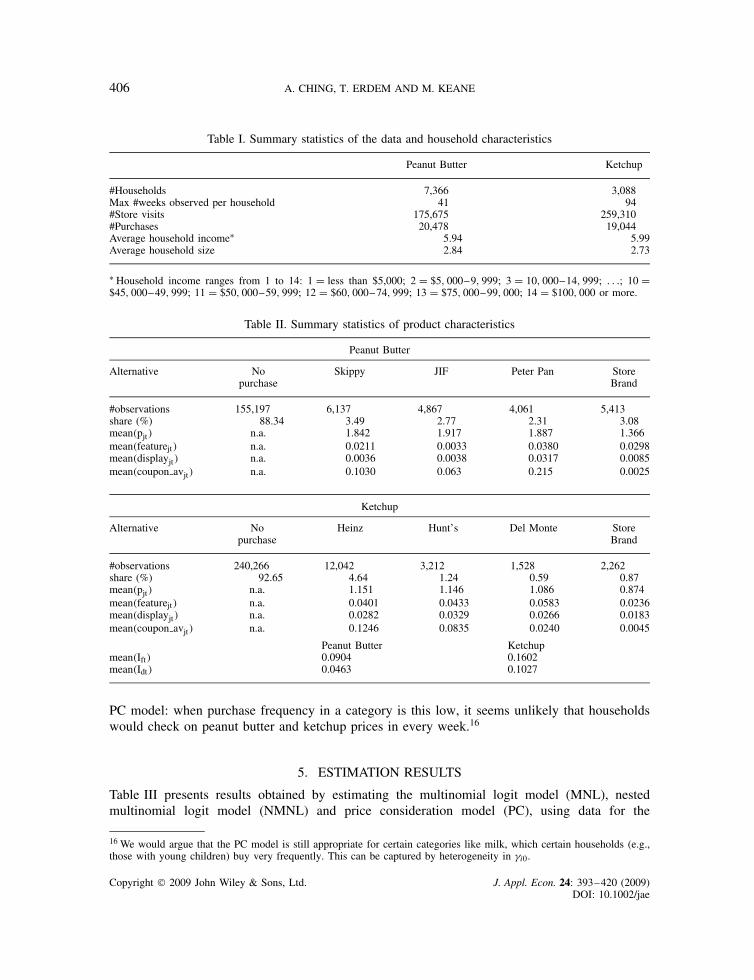
Summary statistics for households are given in Table I, while those for brands are in Table II.Notice that the two categories are rather different. In peanut butter, the four brands have similarmarket shares (ranging from 29.9% for Skippy to 19.8% for Peter Pan), while in ketchup Heinz isdominant (with a market share of 63.1%). Households buy peanut butter and ketchup on 11.66%and 7.35% of shopping occasions, respectively. These figures give face validity to the idea of the
15 The obvious alternative is, on purchase occasions, to use the vector of prices for the size the consumer actually bought,converted to price per ounce. But this begs the question of what price vector to use on occasions when the consumerchose not to buy. Suppose that in non-purchase weeks we use the vector of prices for the most common size (e.g., 32ozfor ketchup), also converted to price per ounce. To see the problem this approach creates, assume there are just two sizes,32oz and 64oz. Furthermore, lets say that on some fraction of purchase occasions consumers buy the 64oz, and that itsprice per ounce tends to be lower. This will introduce a systematic bias whereby the price per ounce vector tends to belower on purchase occasions that on non-purchase occasions (since the average price on purchase occasions is a weightedaverage of 32 and 64 oz prices, while that on non-purchase occasions is just the average 32oz price). Hence, the priceelasticity of demand is exaggerated. It is to avoid this problem that we chose to base the price vector on a common sizefor both purchase and non-purchase occasions.
Copyright 2009 John Wiley & Sons, Ltd. J. Appl. Econ. 24: 393–420 (2009)DOI: 10.1002/jae
406 A. CHING, T. ERDEM AND M. KEANE
Table I. Summary statistics of the data and household characteristics
Peanut Butter Ketchup
#Households 7,366 3,088Max #weeks observed per household 41 94#Store visits 175,675 259,310#Purchases 20,478 19,044Average household incomeŁ 5.94 5.99Average household size 2.84 2.73
Ł Household income ranges from 1 to 14: 1 D less than $5,000; 2 D $5, 000–9, 999; 3 D 10, 000–14, 999; . . .; 10 D$45, 000–49, 999; 11 D $50, 000–59, 999; 12 D $60, 000–74, 999; 13 D $75, 000–99, 000; 14 D $100, 000 or more.
Table II. Summary statistics of product characteristics
Peanut Butter
Alternative Nopurchase
Skippy JIF Peter Pan StoreBrand
#observations 155,197 6,137 4,867 4,061 5,413share (%) 88.34 3.49 2.77 2.31 3.08mean�pjt� n.a. 1.842 1.917 1.887 1.366mean�featurejt� n.a. 0.0211 0.0033 0.0380 0.0298mean�displayjt� n.a. 0.0036 0.0038 0.0317 0.0085mean�coupon avjt� n.a. 0.1030 0.063 0.215 0.0025
Ketchup
Alternative Nopurchase
Heinz Hunt’s Del Monte StoreBrand
#observations 240,266 12,042 3,212 1,528 2,262share (%) 92.65 4.64 1.24 0.59 0.87mean�pjt� n.a. 1.151 1.146 1.086 0.874mean�featurejt� n.a. 0.0401 0.0433 0.0583 0.0236mean�displayjt� n.a. 0.0282 0.0329 0.0266 0.0183mean�coupon avjt� n.a. 0.1246 0.0835 0.0240 0.0045
Peanut Butter Ketchupmean�Ift� 0.0904 0.1602mean�Idt� 0.0463 0.1027
PC model: when purchase frequency in a category is this low, it seems unlikely that householdswould check on peanut butter and ketchup prices in every week.16
5. ESTIMATION RESULTS
Table III presents results obtained by estimating the multinomial logit model (MNL), nestedmultinomial logit model (NMNL) and price consideration model (PC), using data for the
16 We would argue that the PC model is still appropriate for certain categories like milk, which certain households (e.g.,those with young children) buy very frequently. This can be captured by heterogeneity in �i0.
Copyright 2009 John Wiley & Sons, Ltd. J. Appl. Econ. 24: 393–420 (2009)DOI: 10.1002/jae

THE PRICE CONSIDERATION MODEL OF BRAND CHOICE 407
peanut butter category. We estimate two versions of the PC model. In PC-I, decisions toconsider the category depend on category feature and display indicators, the purchase-gap, andhousehold size, while in PC-II these factors influence the utility of the no- purchase option aswell.17
One striking aspect of the results is that coefficient ˛init,GL from equation (30), that captureshow the pre-sample initialized values of the GL variables are related to the brand intercepts, is
Table III. Estimates for the Peanut Butter Category
MNL NMNL PC I PC II
Estimate s.e Estimate s.e. Estimate s.e. Estimate s.e.
˛1 (Store Brand) �5.465 0.148 �6.673 0.212 �3.791 0.078 �4.972 0.158˛2 (JIF) �5.309 0.159 �6.474 0.220 �3.591 0.097 �4.804 0.173˛3 (Peter Pan) �6.003 0.161 �7.217 0.224 �4.317 0.102 �5.499 0.175˛4 (Skippy) �5.115 0.157 �6.251 0.216 �3.387 0.094 �4.596 0.169˛init,GL 106.170 6.061 108.471 5.558 23.548 1.702 25.002 2.223˛init,pg �0.045 0.004 �0.082 0.007 �0.041 0.004 �0.037 0.005
ˇd�displayjt� 1.377 0.054 1.471 0.056 1.728 0.048 1.414 0.055ˇf�featurejt� 2.061 0.039 2.201 0.042 2.259 0.032 2.084 0.040ˇc�coupon avjt� 1.590 0.157 1.986 0.172 1.605 0.164 1.599 0.166ϕp�pjt� �0.239 0.085 �0.346 0.092 �0.846 0.050 �0.226 0.090ϕinc�pjt Ð inci� 0.017 0.003 0.024 0.003 0.018 0.003 0.018 0.003ϕmem�pjt Ð memi� �0.047 0.022 �0.071 0.024 0.112 0.006 �0.071 0.023
State dependence: GLijt D υ Ł GLijt�1 C �1 � υ�Łdijt�1��GLijt� �1.869 0.584 �0.451 0.723 3.179 0.310 2.692 0.320υ 0.989 0.001 0.989 0.001 0.949 0.004 0.953 0.005
Utility of no purchase:ˇfc�Ift� �0.391 0.030 �0.579 0.034 �0.289 0.036ˇdc�Idt� �0.608 0.038 �0.712 0.038 �0.493 0.046ˇmem�memi� �0.306 0.039 �0.309 0.031 �0.330 0.041ˇpg�purch gapit� �0.023 0.002 �0.019 0.001 0.001 0.002
� �0.855 0.122� �D 1/�1 C exp����� 0.702
Probability of considering a category: Pit(C) D exp�Lit�/�1 C exp�Lit�� where: Lit D �i0 C �f РIft C �d РIdt C �mem РmemiC�pg Рpurch gapit , and �i0 D �0 C �initial Рpurch gapi1 C i�0 �1.594 0.140 �1.592 0.162�initial �0.029 0.012 �0.042 0.013�mem 0.118 0.030 0.121 0.033�f 1.376 0.102 1.015 0.107�d 1.748 0.183 1.045 0.157�pg 0.717 0.035 0.868 0.055� 1.163 0.055 1.312 0.088
�log-likelihood 74596.50 74546.882 73983.11 73869.12�2(log-likelihood) 149193.00 149093.764 147966.23 147738.23AIC 149249.00 149151.764 148028.23 147808.23BIC 149539.45 149452.583 148349.79 148171.29
17 The PC-II model nests MNL. By setting Pit�C� D 1 for all i and t, PC-II becomes MNL. Compared with MNL, PC-IIhas five more parameters, which generate Pit�C�. One can send Pit�C� to 1 by sending the mean of �i0 to infinity.
Copyright 2009 John Wiley & Sons, Ltd. J. Appl. Econ. 24: 393–420 (2009)DOI: 10.1002/jae

408 A. CHING, T. ERDEM AND M. KEANE
very large and significant in all the models.18 Thus, the pre-sample purchase behavior conveys agreat deal of information about brand preferences.
Strikingly, there is no evidence for state dependence in the MNL and NMNL models. Thecoefficient on GL is the wrong sign (and insignificant in NMNL), and the parameter υ is close toone, implying a brand purchase hardly moves GL. The PC-I and PC-II models, on the other hand,imply significant state dependence. The coefficients on GL are 2.7 to 3.2, and the estimates implya value of (1 � υ), the coefficient on the purchase dummy, of around. 05. Thus, e.g., in PC-II alagged purchase raises the next period utility for buying a brand by 0.127.
All four models imply similar average price coefficients. The PC-I and PC-II models imply that,for the “average” household the price coefficients are �.421 and �.321, respectively. Thus, e.g.,in PC-II, the effect of a lagged brand purchase on current utility from the brand is equivalent tothe effect of a .127/.321 D 39 cent price reduction. Mean prices are in the $1.36 to $1.92 range,so this is a substantial state dependence effect.
Part of why the PC models imply substantial state dependence while MNL and NMNL do notis that the coefficient ˛init,GL , while still substantial, is smaller in the PC models by a factor of 4.Thus, the MNL and NMNL models ascribe all the pre-sample differences in purchase behavior toheterogeneity, while the PC models do not.
As we would expect, the display, feature and coupon availability variables all have large andhighly significant positive coefficients in the brand specific utility functions in all four models.In the MNL and NMNL models, the utility of the no-purchase option depends negatively on thecategory feature and display indicators, duration since last purchase in the category (purch gap),and on household size. The latter two findings are consistent with inventory behavior. Analogously,in the PC model, the probability of considering the category depends positively on the categoryfeature and display indicators, duration since last purchase in the category, and household size.All these effects are highly significant.
It is useful to examine what the PC models imply about the probability of considering thecategory under different circumstances. Consider a baseline situation with no brand on display orfeature, and a household of size 3 that just bought last period (i.e., purch gapit D 1).19 Then, thePC-II model estimates imply the probability of considering the peanut butter category is 39.7%,on average.20 The estimates of �f and �d are 1.015 and 1.045, respectively. This implies that theconsideration probability increases to 75.6% if one or more brands is on display and feature.21
[Note that, in peanut butter, the category display and feature indicators equal 1 in 4.63% and9.04% of weeks, respectively]. Finally, the estimate of �pg is 0.868. This implies that, startingfrom the baseline, if we increase the purchase gap to 5 weeks, the probability of considering thecategory increases to 90.7%.22
The PC-II model implies that, even conditional on having decided to consider the category, thecategory feature and display indicators, and household size, have significant negative effects on
18 The coefficient ˛init,pg, which captures how the pre-sample purchase gap is related to the brand intercepts, is negativeand significant, as expected. That is, households with a longer initial purchase gap tend to like the entire category less.Hence they have generally lower intercepts, making them more likely to choose the no-purchase option.19 We also specify that the initial value of purch gapi1 was 5. This influences the mean of �0 as in (31).20 We integrate out the unobserved heterogeneity, �i0, when obtaining the average probability of considering.21 That is, when the category display and feature dummies are both set to 1. The predicted effect of feature and displaymay seem high, but it should be emphasized that this is only the probability that a consumer will check the prices ofpeanut butter. After checking prices, the consumer may still choose not to buy in the category.22 The estimate of �mem is 0.121, which implies the effect of household size is fairly small. If we reduce household sizefrom 3 to 1, the consideration probability drops from 39.7% to 35.4%.
Copyright 2009 John Wiley & Sons, Ltd. J. Appl. Econ. 24: 393–420 (2009)DOI: 10.1002/jae

THE PRICE CONSIDERATION MODEL OF BRAND CHOICE 409
utility of no-purchase. The log-likelihood improvement from PC-I to PC-II is 114 points, whileAIC and BIC improve 220 and 179 points, respectively. This suggests feature and display havesome influence on brand choice beyond just drawing attention to the category.23
Finally, we turn to our main goal, which is to investigate whether the PC model fits the databetter than MNL and NMNL. The bottom panel of Table III presents log-likelihood, AIC andBIC values for the four models. The likelihood value for NMNL is modestly better than thatfor MNL (i.e., 50 points). The � on the inclusive value is 0.70, which implies that brandsare closer substitutes than suggested by the MNL model (see equation (9), and recall that if� D 1.0 the models are equivalent). As we discussed in Section 2 and 3.1, NMNL can generatebrand choice price elasticities exceeding those for purchase incidence by assuming brands aresimilar.
However, the log-likelihoods for the PC-I and PC-II models are superior to NMNL by 563.8points and 677.8 points, respectively. The AIC and BIC produce very similar comparisons. Thisis to be expected as the models have similar numbers of parameters (i.e., the MNL, NMNL, PCI-Iand PC-II models have 28, 29, 31 and 35 parameters, respectively). Thus, the PC models clearlyproduce better fits to the peanut butter data than the MNL and NMNL models.
Table IV presents estimates for the ketchup category. Here the estimate of � in the NMNLmodel is essentially 1, so MNL and NMNL are essentially equivalent. Hence, the parametersestimates and likelihood values for MNL and NMNL are essentially the same. The qualitativeresults for ketchup are quite similar to those for peanut butter. One small difference is that, inketchup, MNL and NMNL do generate a positive coefficient � on the GL variable (about 1.3), butit is not statistically significant. Furthermore, the state dependence implied by the point estimatesis very weak. The estimates imply a value of (1 � υ), the coefficient on the purchase dummy, ofaround 0.005. Thus, a lagged purchase raises the next period utility for buying a brand by onlyabout 0.007. As the price coefficient at the mean of the data is �.797, the effect of a laggedpurchase on the current period utility evaluation for a brand is equivalent to a price cut of lessthan 1 cent.
As with peanut butter, the PC models again imply much stronger state dependence. The pricecoefficient for an “average” household is �.964 for PC-I and �.838 for PC-II, which is similarto the values produced by the logit models. But the PC models generate values of � Ð �1 � υ� ofabout �4.3��.028� D .12, so a lagged purchase is comparable to about a .12/.84 D 14 cent pricecut. Mean prices are $0.87 to $1.15, so this is a substantial effect.24
Another difference is that category feature and display variables have positive effects on thevalue of no-purchase in the PC-II model, whereas in peanut butter they had negative effects.Thus, in ketchup, feature and display make a consumer more likely to consider the category, but,conditional on consideration, they make the consumer less likely to actually buy. In peanut butter,they made both consideration and conditional purchase probabilities higher.
To get a sense of how likely a household is to consider ketchup during a store visit, take asituation with no brand on display or feature, and a household of size 3 that bought last period.25
23 The Appendix contains variances and correlations of the brand intercepts. We estimate the Cholesky parameters, butreport the implied variances and correlations, as they are more informative. In peanut butter, the NMNL model implieslarger variances of and larger correlations among the brand specific intercepts than the other models.24 The correlations of the brand specific intercepts in the ketchup category show large positive correlations amongst brands2, 3 and 4 but not with brand 1 (Heinz). This suggests there is basically a Heinz type and a type that regularly buys theother, lower priced, brands.25 As in the peanut butter simulation, we assume the initial value of purch gapi1 D 5, and integrate over �i0.
Copyright 2009 John Wiley & Sons, Ltd. J. Appl. Econ. 24: 393–420 (2009)DOI: 10.1002/jae
410 A. CHING, T. ERDEM AND M. KEANE
Table IV. Estimates for the Ketchup Category
MNL NMNL PC I PC II
Estimate s.e Estimate s.e Estimate s.e Estimate s.e.
˛1 (Heinz) �3.902 0.170 �3.902 0.176 �2.860 0.084 �3.693 0.181˛2 (Hunt’s) �5.251 0.171 �5.252 0.176 �4.084 0.087 �4.915 0.182˛3 (Del Monte) �6.130 0.173 �6.129 0.181 �4.959 0.095 �5.786 0.187˛4 (Store Brand) �5.966 0.166 �5.969 0.174 �4.799 0.082 �5.593 0.182˛init,GL 86.105 7.695 86.245 4.269 16.720 1.921 16.327 1.013˛init,pg �0.037 0.002 �0.037 0.002 �0.030 0.002 �0.031 0.003
ˇd�displayjt� 1.097 0.041 1.097 0.042 1.128 0.032 1.137 0.042ˇf�featurejt� 2.238 0.032 2.238 0.032 2.136 0.024 2.296 0.034ˇc�coupon avjt� 1.583 0.105 1.583 0.107 1.835 0.111 1.836 0.111ϕp�pjt� �1.001 0.148 �1.000 0.154 �1.680 0.080 �0.963 0.154ϕinc�pjt Ð inci� 0.009 0.005 0.009 0.005 0.006 0.005 0.004 0.005ϕmem�pjt Ð memi� 0.055 0.041 0.055 0.042 0.249 0.012 0.037 0.042
State dependence: GLijt D υ Ł GLijt�1 C �1 � υ� Ł dijt�1��GLijt� 1.338 0.800 1.346 0.970 4.235 0.453 4.323 0.438υ 0.995 0.0005 0.995 0.0003 0.973 0.004 0.972 0.002
Utility of no purchase:ˇfc�Ift� �0.037 0.029 �0.037 0.034 0.244 0.035ˇdc�Idt� �0.105 0.034 �0.105 0.038 0.032 0.040ˇmem�memi� �0.217 0.045 �0.217 0.031 �0.259 0.048ˇpg�purch gapit� �0.011 0.001 �0.011 0.001 �0.002 0.001
� �10.212 0.632� �D 1/�1 C exp����� 0.999
Probability of considering a category: Pit(C) D exp�Lit�/�1 C exp�Lit��, where: Lit D �i0 C �f РIft C �d РIdt C �mem РmemiC�pg Рpurch gapit , and �i0 D �0 C �initial Рpurch gapi1 C i�0 �1.043 0.163 �0.937 0.157�initial �0.015 0.008 �0.009 0.008�mem �0.036 0.035 �0.070 0.033�f 1.527 0.107 1.925 0.161�d 1.035 0.141 1.274 0.182�pg 0.475 0.028 0.421 0.025� 0.866 0.114 0.716 0.107
�log-likelihood 71945.204 71945.196 71357.804 71313.949�2(log-likelihood) 143890.408 143890.393 142715.608 142627.899AIC 143946.408 143948.393 142777.608 142697.899BIC 144244.845 144257.489 143108.021 143070.945
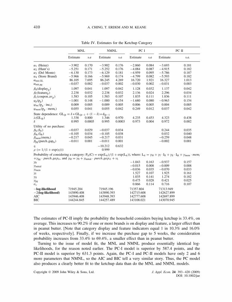
The estimates of PC-II imply the probability the household considers buying ketchup is 33.4%, onaverage. This increases to 90.2% if one or more brands is on display and feature, a larger effect thanin peanut butter. [Note that category display and feature indicators equal 1 in 10.3% and 16.0%of weeks, respectively]. Finally, if we increase the purchase gap to 5 weeks, the considerationprobability increases from 33.4% to 69.4%, a smaller effect than in peanut butter.
Turning to the issue of model fit, the MNL and NMNL produce essentially identical log-likelihoods, for the reason noted earlier. The PC-I model is superior by 587.4 points, and thePC-II model is superior by 631.3 points. Again, the PC-I and PC-II models have only 2 and 6more parameters that NMNL, so the AIC and BIC tell a very similar story. Thus, the PC modelalso produces a clearly better fit to the ketchup data than do the MNL and NMNL models.
Copyright 2009 John Wiley & Sons, Ltd. J. Appl. Econ. 24: 393–420 (2009)DOI: 10.1002/jae
THE PRICE CONSIDERATION MODEL OF BRAND CHOICE 411
6. MODEL SIMULATIONS
6A. Model Simulations: Inter-Purchase Spells
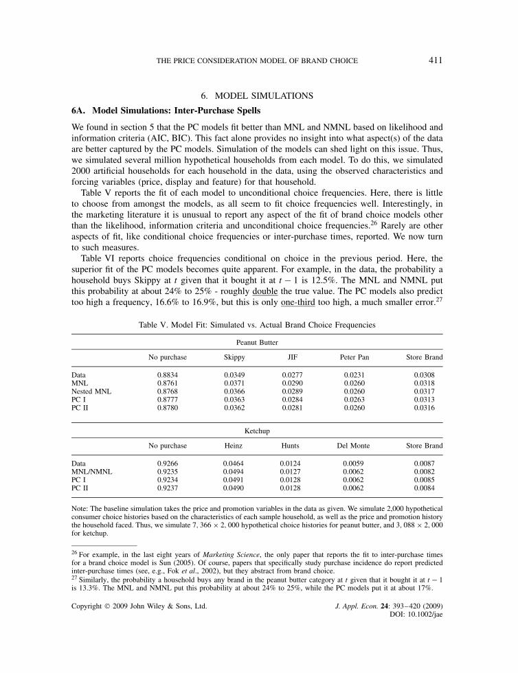
We found in section 5 that the PC models fit better than MNL and NMNL based on likelihood andinformation criteria (AIC, BIC). This fact alone provides no insight into what aspect(s) of the dataare better captured by the PC models. Simulation of the models can shed light on this issue. Thus,we simulated several million hypothetical households from each model. To do this, we simulated2000 artificial households for each household in the data, using the observed characteristics andforcing variables (price, display and feature) for that household.
Table V reports the fit of each model to unconditional choice frequencies. Here, there is littleto choose from amongst the models, as all seem to fit choice frequencies well. Interestingly, inthe marketing literature it is unusual to report any aspect of the fit of brand choice models otherthan the likelihood, information criteria and unconditional choice frequencies.26 Rarely are otheraspects of fit, like conditional choice frequencies or inter-purchase times, reported. We now turnto such measures.
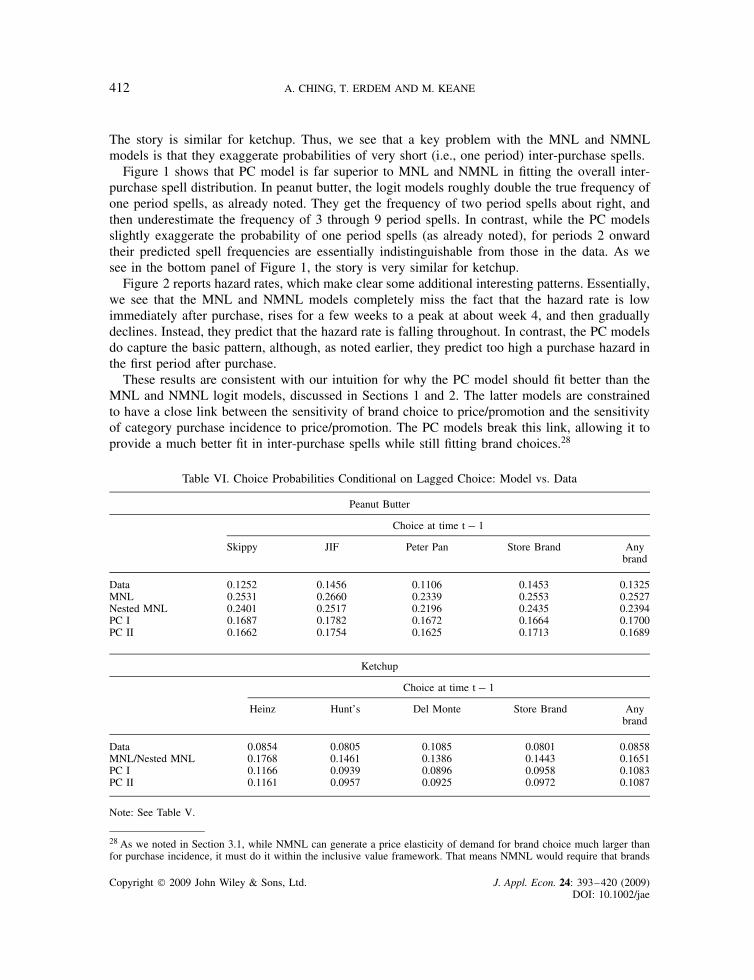
Table VI reports choice frequencies conditional on choice in the previous period. Here, thesuperior fit of the PC models becomes quite apparent. For example, in the data, the probability ahousehold buys Skippy at t given that it bought it at t � 1 is 12.5%. The MNL and NMNL putthis probability at about 24% to 25% - roughly double the true value. The PC models also predicttoo high a frequency, 16.6% to 16.9%, but this is only one-third too high, a much smaller error.27
Table V. Model Fit: Simulated vs. Actual Brand Choice Frequencies
Peanut Butter
No purchase Skippy JIF Peter Pan Store Brand
Data 0.8834 0.0349 0.0277 0.0231 0.0308MNL 0.8761 0.0371 0.0290 0.0260 0.0318Nested MNL 0.8768 0.0366 0.0289 0.0260 0.0317PC I 0.8777 0.0363 0.0284 0.0263 0.0313PC II 0.8780 0.0362 0.0281 0.0260 0.0316
Ketchup
No purchase Heinz Hunts Del Monte Store Brand
Data 0.9266 0.0464 0.0124 0.0059 0.0087MNL/NMNL 0.9235 0.0494 0.0127 0.0062 0.0082PC I 0.9234 0.0491 0.0128 0.0062 0.0085PC II 0.9237 0.0490 0.0128 0.0062 0.0084
Note: The baseline simulation takes the price and promotion variables in the data as given. We simulate 2,000 hypotheticalconsumer choice histories based on the characteristics of each sample household, as well as the price and promotion historythe household faced. Thus, we simulate 7, 366 ð 2, 000 hypothetical choice histories for peanut butter, and 3, 088 ð 2, 000for ketchup.
26 For example, in the last eight years of Marketing Science, the only paper that reports the fit to inter-purchase timesfor a brand choice model is Sun (2005). Of course, papers that specifically study purchase incidence do report predictedinter-purchase times (see, e.g., Fok et al., 2002), but they abstract from brand choice.27 Similarly, the probability a household buys any brand in the peanut butter category at t given that it bought it at t � 1is 13.3%. The MNL and NMNL put this probability at about 24% to 25%, while the PC models put it at about 17%.
Copyright 2009 John Wiley & Sons, Ltd. J. Appl. Econ. 24: 393–420 (2009)DOI: 10.1002/jae
412 A. CHING, T. ERDEM AND M. KEANE
The story is similar for ketchup. Thus, we see that a key problem with the MNL and NMNLmodels is that they exaggerate probabilities of very short (i.e., one period) inter-purchase spells.
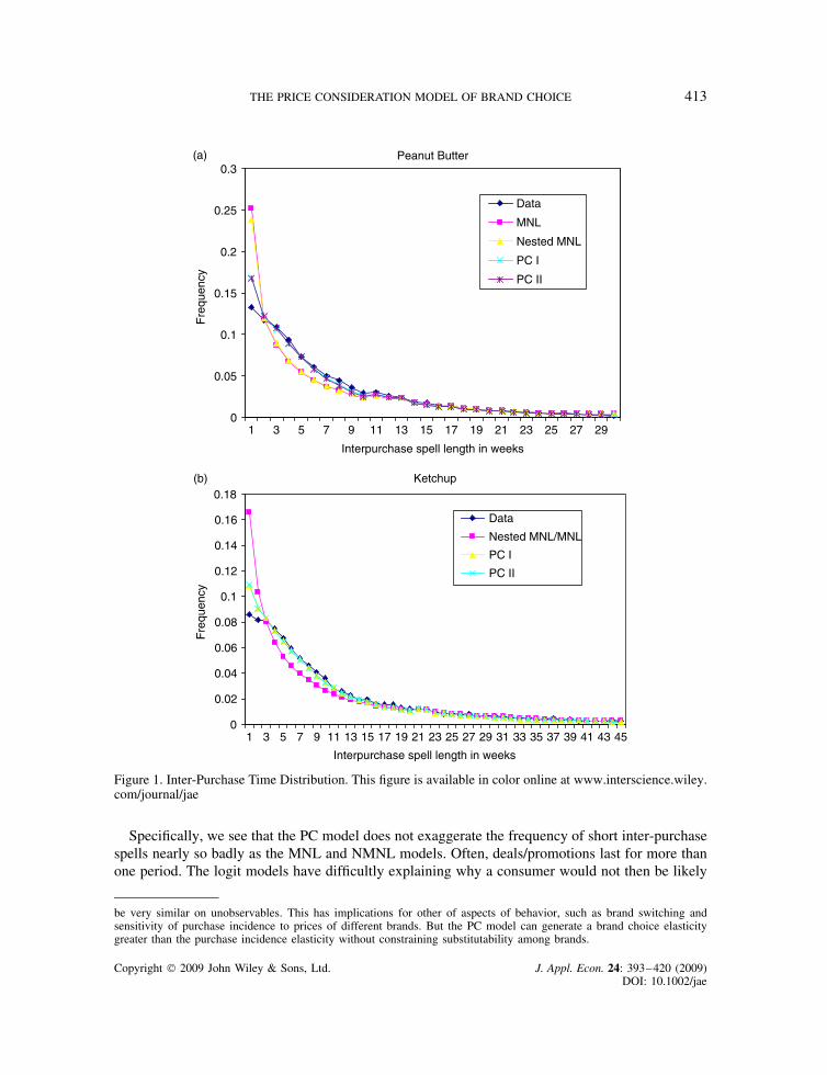
Figure 1 shows that PC model is far superior to MNL and NMNL in fitting the overall inter-purchase spell distribution. In peanut butter, the logit models roughly double the true frequency ofone period spells, as already noted. They get the frequency of two period spells about right, andthen underestimate the frequency of 3 through 9 period spells. In contrast, while the PC modelsslightly exaggerate the probability of one period spells (as already noted), for periods 2 onwardtheir predicted spell frequencies are essentially indistinguishable from those in the data. As wesee in the bottom panel of Figure 1, the story is very similar for ketchup.
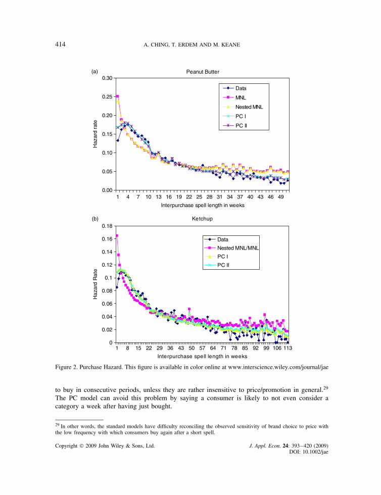
Figure 2 reports hazard rates, which make clear some additional interesting patterns. Essentially,we see that the MNL and NMNL models completely miss the fact that the hazard rate is lowimmediately after purchase, rises for a few weeks to a peak at about week 4, and then graduallydeclines. Instead, they predict that the hazard rate is falling throughout. In contrast, the PC modelsdo capture the basic pattern, although, as noted earlier, they predict too high a purchase hazard inthe first period after purchase.
These results are consistent with our intuition for why the PC model should fit better than theMNL and NMNL logit models, discussed in Sections 1 and 2. The latter models are constrainedto have a close link between the sensitivity of brand choice to price/promotion and the sensitivityof category purchase incidence to price/promotion. The PC models break this link, allowing it toprovide a much better fit in inter-purchase spells while still fitting brand choices.28
Table VI. Choice Probabilities Conditional on Lagged Choice: Model vs. Data
Peanut Butter
Choice at time t � 1
Skippy JIF Peter Pan Store Brand Anybrand
Data 0.1252 0.1456 0.1106 0.1453 0.1325MNL 0.2531 0.2660 0.2339 0.2553 0.2527Nested MNL 0.2401 0.2517 0.2196 0.2435 0.2394PC I 0.1687 0.1782 0.1672 0.1664 0.1700PC II 0.1662 0.1754 0.1625 0.1713 0.1689
Ketchup
Choice at time t � 1
Heinz Hunt’s Del Monte Store Brand Anybrand
Data 0.0854 0.0805 0.1085 0.0801 0.0858MNL/Nested MNL 0.1768 0.1461 0.1386 0.1443 0.1651PC I 0.1166 0.0939 0.0896 0.0958 0.1083PC II 0.1161 0.0957 0.0925 0.0972 0.1087
Note: See Table V.
28 As we noted in Section 3.1, while NMNL can generate a price elasticity of demand for brand choice much larger thanfor purchase incidence, it must do it within the inclusive value framework. That means NMNL would require that brands
Copyright 2009 John Wiley & Sons, Ltd. J. Appl. Econ. 24: 393–420 (2009)DOI: 10.1002/jae
THE PRICE CONSIDERATION MODEL OF BRAND CHOICE 413
Peanut Butter
0
0.05
0.1
0.15
0.2
0.25
0.3
1 3 5 7 9 11 13 15 17 19 21 23 25 27 29
Interpurchase spell length in weeks
Fre
quen
cyData
MNL
Nested MNL
PC I
PC II
Ketchup
0
0.02
0.04
0.06
0.08
0.1
0.12
0.14
0.16
0.18
Interpurchase spell length in weeks
Fre
quen
cy
Data
Nested MNL/MNL
PC I
PC II
1 3 5 7 9 11 13 15 17 19 21 23 25 27 29 31 33 35 37 39 41 43 45
(a)
(b)
Figure 1. Inter-Purchase Time Distribution. This figure is available in color online at www.interscience.wiley.com/journal/jae
Specifically, we see that the PC model does not exaggerate the frequency of short inter-purchasespells nearly so badly as the MNL and NMNL models. Often, deals/promotions last for more thanone period. The logit models have difficultly explaining why a consumer would not then be likely
be very similar on unobservables. This has implications for other of aspects of behavior, such as brand switching andsensitivity of purchase incidence to prices of different brands. But the PC model can generate a brand choice elasticitygreater than the purchase incidence elasticity without constraining substitutability among brands.
Copyright 2009 John Wiley & Sons, Ltd. J. Appl. Econ. 24: 393–420 (2009)DOI: 10.1002/jae
414 A. CHING, T. ERDEM AND M. KEANE
Peanut Butter
0.00
0.05
0.10
0.15
0.20
0.25
0.30
1 4 7 10 13 16 19 22 25 28 31 34 37 40 43 46 49
Interpurchase spell length in weeks
Haz
ard
rate
Ketchup
0
0.02
0.04
0.06
0.08
0.1
0.12
0.14
0.16
0.18
1 8 15 22 29 36 43 50 57 64 71 78 85 92 99 106 113
Interpurchase spell length in weeks
Haz
ard
Rat
e
Data
Nested MNL/MNL
PC I
PC II
Data
MNL
Nested MNL
PC I
PC II
(a)
(b)
Figure 2. Purchase Hazard. This figure is available in color online at www.interscience.wiley.com/journal/jae
to buy in consecutive periods, unless they are rather insensitive to price/promotion in general.29
The PC model can avoid this problem by saying a consumer is likely to not even consider acategory a week after having just bought.
29 In other words, the standard models have difficulty reconciling the observed sensitivity of brand choice to price withthe low frequency with which consumers buy again after a short spell.
Copyright 2009 John Wiley & Sons, Ltd. J. Appl. Econ. 24: 393–420 (2009)DOI: 10.1002/jae
THE PRICE CONSIDERATION MODEL OF BRAND CHOICE 415
Finally, an interesting question is whether the PC model outperforms the MNL/NMNL modelsonly in the aggregate or also in sub-samples. Looking at sub-samples is also a useful way touncover evidence of misspecification. Thus, we looked at subgroups based on city (Sioux Falls vs.Springfield), income (above or below $40,000), household size (above or below 3), and educationof the household head (high-school, some college or college). It was clear that the PC model beatthe MNL/NMNL models in every subgroup, both in terms of the likelihood/AIC/BIC and the fitto the purchase hazard, particularly for very short spells. This was true for both the peanut butterand ketchup categories. We do not report these results in detail in the interest of space, but theyare available upon request.
6B. Model Simulations: Promotion Effects
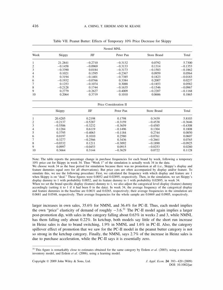
In this section we look at the models’ predictions for the impact of promotions. Table VII reportsthe impact of a temporary 10% price cut for Skippy, and compares the predictions of the NMNLand PC models.30 As price cuts are often accompanied by feature/display activity, we also turnedon 0.5% of the display dummies and 2.9% of the feature dummies, as described in detail in thefootnote to the table.
The similarity of the models’ predictions is remarkable. The PC-II model predicts a 20.4%increase in Skippy sales in the week of the promotion, while the NMNL model predicts a 21.3%increase. Thus, both models imply short run “price” elasticities of demand of roughly �2, althoughit should be stressed this is not a conventional price elasticity because we include the additionalpromotion activity that typically accompanies a price cut.
Each model implies little brand switching. The NMNL and PC-II models imply that totalcategory sales increase by 5.7% and 5.8%, respectively. The NMNL says 98% of the increasein Skippy sales is from category expansion, while only 2% is switching from other brands. ThePC-II model actually says that sales of the other brands increase slightly (about 0.2 to 0.3%), soall the increased Skippy sales is from category expansion. This phenomenon is a spillover effectof promotion that arises in the PC models. If one brand uses features and/or displays, it can attracta consumer’s attention to the category, but, when he/she checks out prices, he/she may decide tobuy some other brand besides the one that was promoted.
We can also examine the long run effects of the price cut. Their sign is theoretically ambiguous.A price cut may lead to purchase acceleration, where a consumer buys today rather than waitingto buy in a future period (an inventory planning phenomenon). On the other hand, increased salestoday can lead to greater future sales through habit persistence/enhanced brand equity, capturedby the GL variables.
The NMNL and PC-II make opposite predictions about the direction of these effects, but bothagree they are small. According to NMNL, the drop in Skippy sales in weeks 2 through 10cancels out 3.4% of the increased sales created by the price cut. In contrast, PC-II says Skippysales increase by roughly 0.52% in weeks 2 through 10. A notable difference between the modelsis that PC-II implies a post-promotion dip for all brands in weeks 2 to 3, with total category salesfalling about 0.4% in each week. The comparable figure for NMNL is only bout 0.16%.
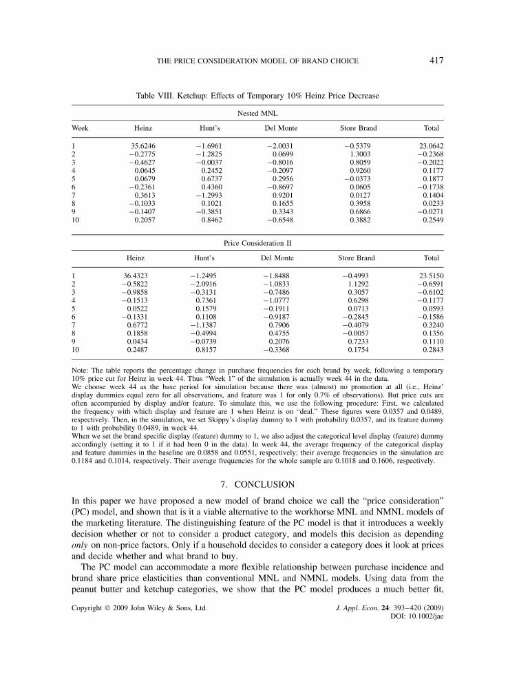
The results for ketchup are a bit different. When we simulate a 10% price cut for Heinz,accompanied by turning on display (feature) with a probability of 3.6% (4.9%), we get much
30 The MNL and PC-I models make similar predictions, so we do not report them. They are available on request.
Copyright 2009 John Wiley & Sons, Ltd. J. Appl. Econ. 24: 393–420 (2009)DOI: 10.1002/jae
416 A. CHING, T. ERDEM AND M. KEANE
Table VII. Peanut Butter: Effects of Temporary 10% Price Decrease for Skippy
Nested MNL
Week Skippy JIF Peter Pan Store Brand Total
1 21.2841 �0.2710 �0.3132 0.0792 5.73002 �0.1458 �0.0969 �0.3133 0.1314 �0.13533 �0.3390 0.0184 �0.3173 �0.1583 �0.18624 0.1021 0.1595 �0.2367 0.0959 0.05645 0.3194 �0.1401 �0.7385 0.1823 �0.01836 �0.1932 �0.0766 0.3384 0.2007 0.02377 0.1253 �0.1074 0.3088 �0.1853 0.05828 �0.2128 0.1744 �0.1635 �0.1546 �0.09679 0.2779 �0.2627 �0.4009 �0.2207 �0.116810 0.2064 0.3719 0.1010 0.0686 0.1865
Price Consideration II
Skippy JIF Peter Pan Store Brand Total
1 20.4285 0.2198 0.1798 0.3439 5.81032 �0.2137 �0.5287 �0.3159 �0.4538 �0.36463 �0.5506 �0.3232 �0.3659 �0.4585 �0.43084 0.1284 0.6119 �0.1496 0.1304 0.18085 0.3795 �0.4063 �0.1184 0.2744 0.08506 0.0197 0.1010 0.2580 �0.0761 0.06077 0.3277 �0.2566 0.3436 �0.2661 0.07658 �0.0332 0.1211 �0.3092 �0.1890 �0.09259 0.0997 �0.0453 0.0915 �0.0253 0.028010 0.3664 0.3144 �0.3629 0.0722 0.1128
Note: The table reports the percentage change in purchase frequencies for each brand by week, following a temporary10% price cut for Skippy in week 34. Thus “Week 1” of the simulation is actually week 34 in the data.We choose week 34 as the base period for simulation because there was no promotion at all (i.e., Skippy’s display andfeature dummies equal zero for all observations). But price cuts are often accompanied by display and/or feature. Tosimulate this, we use the following procedure: First, we calculated the frequency with which display and feature are 1when Skippy is on “deal.” These figures were 0.0052 and 0.02895, respectively. Then, in the simulation, we set Skippy’sdisplay dummy to 1 with probability 0.0052, and its feature dummy to 1 with probability 0.02895, in week 34.When we set the brand specific display (feature) dummy to 1, we also adjust the categorical level display (feature) dummyaccordingly (setting it to 1 if it had been 0 in the data). In week 34, the average frequency of the categorical displayand feature dummies in the baseline are 0.0631 and 0.0265, respectively; their average frequencies in the simulation are0.0681 and 0.0548, respectively. Their average frequencies for the whole sample are 0.0469 and 0.0905, respectively.
larger increases in own sales, 35.6% for NMNL and 36.4% for PC-II. Thus, each model impliesthe own “price” elasticity of demand of roughly �3.6.31 The PC-II model again implies a largerpost-promotion dip, with sales in the category falling about 0.63% in weeks 2 and 3, while NMNLhas them falling only about 0.22%. In ketchup, both models say little of the short run increasein Heinz sales is due to brand switching, 1.9% in NMNL and 1.6% in PC-II. Also, the categoryspillover effect of promotion that we saw for the PC-II model in the peanut butter category is notso strong in the ketchup category. Finally, the NMNL says 2.7% of the increase in Heinz sales isdue to purchase acceleration, while the PC-II says it is essentially zero.
31 This figure is remarkably close to estimates obtained for the same category by Erdem et al. (2003), using a structuralinventory model, and Erdem et al. (2006), using a learning model.
Copyright 2009 John Wiley & Sons, Ltd. J. Appl. Econ. 24: 393–420 (2009)DOI: 10.1002/jae
THE PRICE CONSIDERATION MODEL OF BRAND CHOICE 417
Table VIII. Ketchup: Effects of Temporary 10% Heinz Price Decrease
Nested MNL
Week Heinz Hunt’s Del Monte Store Brand Total
1 35.6246 �1.6961 �2.0031 �0.5379 23.06422 �0.2775 �1.2825 0.0699 1.3003 �0.23683 �0.4627 �0.0037 �0.8016 0.8059 �0.20224 0.0645 0.2452 �0.2097 0.9260 0.11775 0.0679 0.6737 0.2956 �0.0373 0.18776 �0.2361 0.4360 �0.8697 0.0605 �0.17387 0.3613 �1.2993 0.9201 0.0127 0.14048 �0.1033 0.1021 0.1655 0.3958 0.02339 �0.1407 �0.3851 0.3343 0.6866 �0.027110 0.2057 0.8462 �0.6548 0.3882 0.2549
Price Consideration II
Heinz Hunt’s Del Monte Store Brand Total
1 36.4323 �1.2495 �1.8488 �0.4993 23.51502 �0.5822 �2.0916 �1.0833 1.1292 �0.65913 �0.9858 �0.3131 �0.7486 0.3057 �0.61024 �0.1513 0.7361 �1.0777 0.6298 �0.11775 0.0522 0.1579 �0.1911 0.0713 0.05936 �0.1331 0.1108 �0.9187 �0.2845 �0.15867 0.6772 �1.1387 0.7906 �0.4079 0.32408 0.1858 �0.4994 0.4755 �0.0057 0.13569 0.0434 �0.0739 0.2076 0.7233 0.111010 0.2487 0.8157 �0.3368 0.1754 0.2843
Note: The table reports the percentage change in purchase frequencies for each brand by week, following a temporary10% price cut for Heinz in week 44. Thus “Week 1” of the simulation is actually week 44 in the data.We choose week 44 as the base period for simulation because there was (almost) no promotion at all (i.e., Heinz’display dummies equal zero for all observations, and feature was 1 for only 0.7% of observations). But price cuts areoften accompanied by display and/or feature. To simulate this, we use the following procedure: First, we calculatedthe frequency with which display and feature are 1 when Heinz is on “deal.” These figures were 0.0357 and 0.0489,respectively. Then, in the simulation, we set Skippy’s display dummy to 1 with probability 0.0357, and its feature dummyto 1 with probability 0.0489, in week 44.When we set the brand specific display (feature) dummy to 1, we also adjust the categorical level display (feature) dummyaccordingly (setting it to 1 if it had been 0 in the data). In week 44, the average frequency of the categorical displayand feature dummies in the baseline are 0.0858 and 0.0551, respectively; their average frequencies in the simulation are0.1184 and 0.1014, respectively. Their average frequencies for the whole sample are 0.1018 and 0.1606, respectively.
7. CONCLUSION
In this paper we have proposed a new model of brand choice we call the “price consideration”(PC) model, and shown that is it a viable alternative to the workhorse MNL and NMNL models ofthe marketing literature. The distinguishing feature of the PC model is that it introduces a weeklydecision whether or not to consider a product category, and models this decision as dependingonly on non-price factors. Only if a household decides to consider a category does it look at pricesand decide whether and what brand to buy.
The PC model can accommodate a more flexible relationship between purchase incidence andbrand share price elasticities than conventional MNL and NMNL models. Using data from thepeanut butter and ketchup categories, we show that the PC model produces a much better fit,
Copyright 2009 John Wiley & Sons, Ltd. J. Appl. Econ. 24: 393–420 (2009)DOI: 10.1002/jae
418 A. CHING, T. ERDEM AND M. KEANE
particularly to inter-purchase spells. The standard models greatly overstate the frequency of shortspells, because they have difficulty reconciling the observed high sensitivity of brand shares toprice with low sensitivity of purchase incidence to price in the period shortly after a purchase(when inventory is high). Moreover, the PC model is as simple to estimate as standard models.
ACKNOWLEDGEMENTS
Ching’s work on this project was supported by Connaught Start-up Grant at the Universityof Toronto. Keane’s work on this project was supported by NSF grants SBR-9511280 andSBR-9812067, and ARC grant FF0561843. The authors thank (without intending to implicate)participants in the marketing and economics seminars at Duke University, the 2006 MarketingScience Conference, the 2006 Marketing Dynamics Conference and the 7th Invitational ChoiceSymposium held at Wharton in June 2007 (especially Michael Hanemann and Bob Meyer), forhelpful comments.
REFERENCES
Berry S, Levinshon J, Pakes A. 1995. Automobile Prices in Market Equilibrium. Econometrica 63: 841–890.Erdem T, Imai S, Keane M. 2003. Brand and Quantity Choice Dynamics Under Price Uncertainty. Quanti-
tative Marketing and Economics 1: 5–64.Erdem T, Keane M, Sun B. 1999. Missing Price and Coupon Availability Data in Scanner Panels: Correcting
for the Self-Selection Bias in the Choice Model Parameters. Journal of Econometrics 89: 177–196.Erdem T, Keane M, Sun B. 2006. A Dynamic Model of Brand Choice When Price and Advertising Signal
Product Quality, Marketing Science, 27: 1111–1125.Fok D, Paap R, Franses PH. 2002. Modeling Dynamic Effects of Promotion on Interpurchase Times.
Econometric Institute Report EI 2002/37.Guadagni PM, Little JDC. 1983. A Logit Model of Brand Choice Calibrated on Scanner Data. Marketing
Science 2: 203–238.Harris K, Keane M. 1999. A Model of Health Plan Choice: Inferring Preferences and Perceptions from a
Combination of Revealed Preference and Attitudinal Data. Journal of Econometrics 89: 131–157.Heckman J. 1981. The Incidental Parameters Problem and the Problem of Initial Conditions in Estimating
a Discrete Time-Discrete Data Stochastic Process. In Structural Analysis of Discrete Data with EconomicApplications, Manski C, McFadden D (eds). MIT: Cambridge, MA.
Helsen K, Schmittlein DC. 1993. Analyzing Duration Times in Marketing: Evidence for the Effectivenessof Hazard Rate Models. Marketing Science 12: 395–414.
Hendel I, Nevo A. 2003. Measuring the Implications of Sales and Consumer Stockpiling. Working paper,Northwestern University.
Keane M. 1993. Simulation Estimation for Panel Data Models with Limited Dependent Variables. InHandbook of Statistics, Maddala GS, Rao CR, Vinod HD (eds). Elsevier Science Publishers: New York.
Keane M. 1994. A Computationally Practical Simulation Estimator for Panel Data. Econometrica 62: 95–116.Keane M. 1997a. Current Issues in Discrete Choice Modeling. Marketing Letters 8: 307–322.Keane M. 1997b. Modeling Heterogeneity and State Dependence in Consumer Choice Behavior. Journal of
Business and Economic Statistics 15: 310–326.Maddala GS. 1983. Limited-dependent and Qualitative Variables in Econometrics. University Press: Cam-
bridge.McFadden D. 1978. Modeling the Choice of Residential Location. In Spatial Interaction Theory and
Residential Location, Karlquist A (ed). North Holland: Amsterdam; 75–96.McFadden D. 1989. A Method of Simulated Moments for Estimation of Discrete Choice Response Models
Without Numerical Integration. Econometrica 57: 995–1026.Pakes A. 1986. Patents as Options: Some Estimates of the Value of Holding European Patent Stocks.
Econometrica 54: 755–84.
Copyright 2009 John Wiley & Sons, Ltd. J. Appl. Econ. 24: 393–420 (2009)DOI: 10.1002/jae
THE PRICE CONSIDERATION MODEL OF BRAND CHOICE 419
Sun B, Neslin S, Srinivasan K. 2003. Measuring the Impact of Promotions on Brand Switching WhenConsumers Are Forward-looking. Journal of Marketing Research 40: 389–405.
Sun B. 2005. Promotion Effect on Endogenous Consumption. Marketing Science 3: 430–443.Wooldridge J. 2003a. Econometric Analysis of Cross Section and Panel Data. MIT Press: Cambridge, MA.Wooldridge J. 2003b. Simple Solutions to the Initial Conditions Problem in Dynamic, Nonlinear Panel Data
Models with Unobserved Heterogeneity. Working Paper, Michigan State University.
Copyright 2009 John Wiley & Sons, Ltd. J. Appl. Econ. 24: 393–420 (2009)DOI: 10.1002/jae
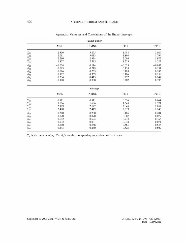
420 A. CHING, T. ERDEM AND M. KEANE
Appendix: Variances and Correlations of the Brand Intercepts
Peanut Butter
MNL NMNL PC I PC II
11 2.356 3.275 1.988 2.02922 2.091 3.013 1.808 1.79933 2.210 2.934 2.003 1.97544 1.857 2.595 1.523 1.523
21 �0.054 0.114 �0.023 �0.053 31 0.093 0.219 0.135 0.131 32 0.086 0.233 0.183 0.183 41 0.192 0.369 0.186 0.159 42 0.234 0.413 0.272 0.247 43 0.128 0.300 0.207 0.193
Ketchup
MNL NMNL PC I PC II
11 0.811 0.811 0.636 0.66422 1.696 1.696 1.545 1.57133 2.179 2.177 2.045 2.05744 2.420 2.419 2.319 2.243
21 0.200 0.200 0.185 0.204 31 0.070 0.070 0.067 0.077 32 0.692 0.694 0.773 0.766 41 0.032 0.031 0.038 0.074 42 0.390 0.388 0.561 0.536 43 0.443 0.440 0.525 0.509
jj is the variance of ˛ij. The ij’s are the corresponding correlation matrix elements.
Copyright 2009 John Wiley & Sons, Ltd. J. Appl. Econ. 24: 393–420 (2009)DOI: 10.1002/jae