Technical Report Documentation Page 1. Report No. FHWA/TX-13/0-6607-2

2. Government Accession No.

3. Recipient's Catalog No.

4. Title and Subtitle THE OVERLAY TESTER (OT): COMPARISON WITH OTHER CRACK TEST METHODS AND RECOMMENDATIONS FOR SURROGATE CRACK TESTS

5. Report Date October 2012 Published: August 2013 6. Performing Organization Code

7. Author(s) Lubinda F. Walubita, Abu N. Faruk, Yasser Koohi, Rong Luo, Tom Scullion, and Robert L. Lytton

8. Performing Organization Report No. Report 0-6607-2

9. Performing Organization Name and Address Texas A&M Transportation Institute College Station, Texas 77843-3135

10. Work Unit No. (TRAIS) 11. Contract or Grant No. Project 0-6607

12. Sponsoring Agency Name and Address Texas Department of Transportation Research and Technology Implementation Office P. O. Box 5080 Austin, Texas 78763-5080

13. Type of Report and Period Covered Technical Report: September 2010–September 2012 14. Sponsoring Agency Code

15. Supplementary Notes Project performed in cooperation with the Texas Department of Transportation and the Federal Highway Administration. Project Title: Search for a Test for Fracture Potential of Asphalt Mixes URL: http://tti.tamu.edu/documents/0-6607-2.pdf 16. Abstract

Presently, one of the principal performance concerns of hot-mix asphalt (HMA) pavements is premature cracking, particularly of HMA surfacing mixes. Regrettably, however, while many USA transportation agencies have implemented design-level tests to measure the rutting potential of HMA mixes; there is hardly any standardized national design-level test for measuring and characterizing the HMA cracking resistance potential. Currently, the Texas Department of Transportation (TxDOT) uses the Overlay Tester (OT) to routinely evaluate the cracking susceptibility of HMA mixes in the laboratory. While the OT effectively simulates the reflective cracking mechanism of opening and closing of joints and/or cracks, repeatability and variability in the test results have been major areas of concern.

As an effort towards addressing these repeatability/variability issues, this laboratory study was undertaken, namely to: 1) conduct a comprehensive sensitivity evaluation of the OT test procedure so as to improve its repeatability and minimize variability in the OT test results; 2) recommend updates and modifications to the Tex-248-F specification including development of OT calibration and service maintenance manuals; 3) explore other alternative OT data analysis methods; 4) comparatively evaluate and explore other crack test methods (both in monotonic and dynamic loading modes) that could serve as supplementary and/or surrogate tests to the OT test method; and 5) develop new crack test procedures, specifications, and technical implementation recommendations.

As documented in this report, the scope of work to accomplish these objectives included evaluating the following crack test methods: 1) the standard repeated (OTR, Tex-248-F) and monotonic loading OT test (OTM); 2) the monotonic (IDT) and repeated loading indirect-tension (R-IDT) test; 3) the monotonic (SCB) and repeated loading semi-circular bending (R-SCB) test; 4) the disk-shaped compaction tension test (DSCTT); and 5) the monotonic (DT) and repeated loading direct-tension (R-DT) tests.

17. Key Words HMA, Cracking, Repeatability, Variability, Coefficient of Variation, Overlay Tester (OTR), Monotonic OT (OTM), Indirect Tension (IDT, R-IDT), Semi-Circular Bending (SCB, R-SCB), Disk-Shaped Compaction Tension Test (DSCTT), Fracture Energy (FE), FE Index, Cycle Index

18. Distribution Statement No restrictions. This document is available to the public through NTIS: National Technical Information Service Alexandria, Virginia 22312 http://www.ntis.gov

19. Security Classif. (of this report) Unclassified

20. Security Classif. (of this page) Unclassified

21. No. of Pages 180

22. Price

Form DOT F 1700.7 (8-72) Reproduction of completed page authorized

THE OVERLAY TESTER (OT): COMPARISON WITH OTHER CRACK TEST METHODS AND RECOMMENDATIONS FOR SURROGATE CRACK TESTS

by

Lubinda F. Walubita Research Scientist

Texas A&M Transportation Institute

Abu N. Faruk Research Associate

Texas A&M Transportation Institute

Yasser Koohi Graduate Research Assistant

Texas A&M Transportation Institute

Rong Luo Associate Research Engineer

Texas A&M Transportation Institute

Tom Scullion Senior Research Engineer

Texas A&M Transportation Institute

Robert L. Lytton Research Engineer

Texas A&M Transportation Institute

Report 0-6607-2 Project 0-6607

Project Title: Search for a Test for Fracture Potential of Asphalt Mixes

Performed in cooperation with the Texas Department of Transportation

and the Federal Highway Administration

October 2012 Published: August 2013

TEXAS A&M TRANSPORTATION INSTITUTE College Station, Texas 77843-3135

v

DISCLAIMER

The contents of this report reflect the views of the authors, who are responsible for the

facts and the accuracy of the data presented herein. The contents do not necessarily reflect the

official view or policies of the Federal Highway Administration (FHWA) or the Texas

Department of Transportation (TxDOT). This report does not constitute a standard, specification,

or regulation, nor is it intended for construction, bidding, or permit purposes. The United States

Government and the State of Texas do not endorse products or manufacturers. Trade or

manufacturers’ names appear herein solely because they are considered essential to the object of

this report. The engineer in charge was Tom Scullion, P.E. #62683.

vi

ACKNOWLEDGMENTS

This project was conducted for TxDOT, and the authors thank TxDOT and FHWA for

their support in funding this research project. In particular, the guidance and technical assistance

of the project director, Richard Izzo, P.E., of TxDOT, proved invaluable. The following project

advisors also provided valuable input throughout the course of the project: Karl Bednarz, Miles

Garrison, Ronald Hatcher, Feng Hong, Martin Kalinowski, and Stephen Smith.

The authors extend their special appreciation to Gautam Das, Hossain Tanvir, Jason

Huddleston, Guillermo Ramos, Jacob Hoeffner, Carlos Flores, Lee Gustavus, and Tony Barbosa

from the Texas A&M Transportation Institute (TTI) for their help with laboratory and field

work. Likewise, thanks to Brett Haggerty and Thomas Smith of TxDOT-CST for their assistance

with laboratory testing at the TxDOT-CST lab.

The following TxDOT lab personnel are also acknowledged for their assistance with the

round-robin testing: Ronald Hatcher (Childress), Hop-Ming Tang (Houston), and Josiah Yuen

(Houston). The following TxDOT individuals and institutions are gratefully thanked for

supplying both the plant-mix and raw materials for lab testing: Ramon Rodriquez (Laredo),

Chico TxDOT District Lab, Miles Garrison (Atlanta), Bryan District Office, Waco, Odessa, and

Fort Worth.

vii

TABLE OF CONTENTS

List of Figures ............................................................................................................................... ix

List of Tables ................................................................................................................................. x

List of Notations and Symbols .................................................................................................. xiii Chapter 1: Introduction ............................................................................................................ 1-1

Research Objectives and Scope of Work ................................................................................. 1-2 Research Methodology and Work Plans .................................................................................. 1-2 Report Contents and Organizational Layout ............................................................................ 1-3 Summary ................................................................................................................................... 1-4

Chapter 2: Experimental Design Plan and HMA Mixes ........................................................ 2-1 Materials and HMA Mix-Designs ............................................................................................ 2-1 HMA Specimen Fabrication ..................................................................................................... 2-3 Summary ................................................................................................................................. 2-55

Chapter 3: The TEX-248-F Specification and OT Test Procedure ....................................... 3-1 OT Sensitivity Evaluation and TEX-248-F Updates ................................................................ 3-1 OT Round-Robin Testing and Operator Effect ........................................................................ 3-9 OT Software, Calibration, and Maintenance .......................................................................... 3-13 Summary ................................................................................................................................. 3-18

Chapter 4: The OT Test Method – Dynamic and Monotonic Loading Modes .................... 4-1 Test Setup ................................................................................................................................. 4-1 Test Response Curves and Data Analysis ................................................................................ 4-4 The OTM and OTR Test Results ................................................................................................ 4-7 Comparison of the OTM and OTR Test Methods .................................................................... 4-14 Summary ................................................................................................................................. 4-15

Chapter 5: The IDT and R-IDT Test Methods ....................................................................... 5-1 TEST SETUP ........................................................................................................................... 5-1 Test Response Curves and Data Analysis Models ................................................................... 5-4 IDT and R-IDT Test Results .................................................................................................... 5-7 Comparison of the IDT and R-IDT Test Methods ................................................................. 5-15 Summary ................................................................................................................................. 5-15

Chapter 6: The SCB and R-SCB Test Methods ...................................................................... 6-1 Test Setup ................................................................................................................................. 6-1 Test Response Curves and Data Analysis Models ................................................................... 6-3 SCB and R-SCB Test Results ................................................................................................... 6-6 Comparison of the SCB and R-SCB Test Methods ................................................................ 6-13 Summary ................................................................................................................................. 6-14

Chapter 7: The DSCTT Test Method ...................................................................................... 7-1 The DSCTT Test Procedure ..................................................................................................... 7-1 The DSCTT Data Analysis Models .......................................................................................... 7-2 DSCTT Test Results ................................................................................................................. 7-4 Other Data Analysis and Test Methods Evaluated ................................................................... 7-5 Summary ................................................................................................................................... 7-6

viii

Chapter 8: Comparison of the Crack Test Methods .............................................................. 8-1 HMA Crack Tests Evaluated .................................................................................................... 8-1 Test Loading Parameters and Output Data ............................................................................... 8-1 Loading Configuration and Specimen Failure Modes .............................................................. 8-3 Test Repeatability and Load-Displacement Response Curves ................................................. 8-5 Potential to Differentiate and Screen Mixes ............................................................................. 8-7 Sensitivity to HMA Mix-Design Variables .............................................................................. 8-8 Case Studies and Field Correlations ....................................................................................... 8-11 Comparative Evaluation and Ranking of the Test Methods ................................................... 8-13 Summary ................................................................................................................................. 8-14

Chapter 9: Summary, Conclusions, and Recommendations ................................................. 9-1 OT Sensitivity Evaluation ........................................................................................................ 9-1 Supplementary and Surrogate Crack Tests ............................................................................... 9-2

References .................................................................................................................................. R-1

Appendix A: OT Machine Check, Calibration, and Verification prior to Round-Robin Testing ................................................................................................................ A-1

Appendix B: OT Parallel Testing with TxDOT-CST (Austin) ............................................. B-1

Appendix C: Load-Displacement Response Curves for Monotonic Loading Crack Tests ................................................................................................................................ C-1

Appendix D: Advanced OT Data Analysis Methods Using Energy Concept and Numerical Modeling ..................................................................................................... D-1

Appendix E: The DT and R-DT Test Methods ...................................................................... E-1

ix

LIST OF FIGURES

Figure 3-1. Effects of Displacement Variations at Constant Frequency – 10 Sec/Cycle. ........... 3-4 Figure 3-2. Loading Frequency Variations at Constant Displacement – 0.025 Inches. .............. 3-5 Figure 3-3. Effects of Sample Notching on the OT Results. ....................................................... 3-6 Figure 3-4. Single and Multiple Cracking in Some OT Samples. ............................................... 3-7 Figure 3-5. The New OT Calibration Kit and Examples of Linear Graphical Screen Plots. ..... 3-15 Figure 3-6. Typical Load-Voltage Response Curve – Well-Calibrated OT Load Cell. ............ 3-16 Figure 3-7. OT Verification of the Raw Data Files. .................................................................. 3-17 Figure 4-1. Overlay Tester (OT) Setup. ....................................................................................... 4-2 Figure 4-2. Load-Displacement Response Curve: OTM Testing. ................................................ 4-4 Figure 4-3. OTR Output Data and Interpretation of Results. ....................................................... 4-6 Figure 4-4. Comparison of HMA Mixes Based on OTM and OTR Test Results.......................... 4-8 Figure 4-5. Relationship between the OTR Cycles and OTM FE Index. ...................................... 4-9 Figure 4-6. OTM and OTR Test Parameter Sensitivity to AC Variation. ................................... 4-12 Figure 5-1. IDT Horizontal Displacement Calculation from Vertical (Ram)

Displacements. ................................................................................................................. 5-3 Figure 5-2. Load-Displacement Response Curve: IDT Testing. ................................................. 5-5 Figure 5-3. R-IDT Load (Input) – Displacement (Output) Curve. .............................................. 5-6 Figure 5-4. Evolution of Peak Displacement with the Number of Load Cycles. ........................ 5-7 Figure 5-5. IDT Test Outputs: Load-Displacement Response Curves. ....................................... 5-8 Figure 5-6. Summary of IDT Test Results................................................................................... 5-9 Figure 5-7. IDT and R-IDT Test Parameter Sensitivity to AC Variation. ................................. 5-13 Figure 6-1. Load-Displacement Response Curve: SCB Testing. ................................................ 6-4 Figure 6-2. R-SCB Load (Input) – Displacement (Output) Curve. ............................................. 6-5 Figure 6-3. Evolution of Peak Displacement with the Number of Load Cycles. ........................ 6-6 Figure 6-4. SCB Test Outputs: Load-Displacement Response Curves. ...................................... 6-7 Figure 6-5. Summary of SCB Test Results. ................................................................................. 6-8 Figure 6-6. SCB and R-SCB Test Parameter Sensitivity to AC Variation. ............................... 6-12 Figure 6-7. SCB and R-SCB Testing at High AC Levels: Multiple Crack Failure Modes. ...... 6-13 Figure 7-1. DSCTT Testing Setup and Specimen Dimensions. .................................................. 7-1 Figure 7-2. Load-Displacement Response Curve: DSCTT Testing. ........................................... 7-3 Figure 7-3. DSCTT Load-Displacement Response Curve: Type D (5.5% AC). ......................... 7-4 Figure 8-1. Multiple Cracking in OTR, SCB, and R-SCB Tests. ................................................. 8-5 Figure 8-2. Comparison of Test Repeatability (Load-Displacement Response Curves). ............ 8-7

x

LIST OF TABLES

Table 2-1. Materials and Mix-Design Characteristics. ................................................................ 2-2 Table 2-2. HMA Mixing and Compaction Temperatures. ........................................................... 2-4 Table 3-1. OT Sensitivity Evaluation and Recommendations for Tex-248-F Updates. .............. 3-2 Table 3-2. OT Sample Thickness Variation Results. ................................................................... 3-3 Table 3-3. Alternative OT Data Analysis Methods (Walubita et al., 2012). ............................... 3-9 Table 3-4. OT Round-Robin Results – Laredo Type C Mix. .................................................... 3-10 Table 3-5. OT Round-Robin Results – Four Different HMA Mixes. ........................................ 3-10 Table 3-6. OT Operator Effect. .................................................................................................. 3-11 Table 3-7. Trained Operator Effect. ........................................................................................... 3-11 Table 3-8. Trained Operator and Equipment Effect. ................................................................. 3-12 Table 3-9. OT Results – New (Version 1.9.0) versus Old Software. ........................................ 3-14 Table 4-1. OTM and OTR Test Parameters. .................................................................................. 4-1 Table 4-2. OT Results Summary. ................................................................................................ 4-7 Table 4-3. Screening of HMA Mixes Based on Discriminatory Ratios. ................................... 4-10 Table 4-4. Screening of HMA Mixes Based on ANOVA and Tukey’s HSD Analysis. ........... 4-11 Table 4-5. Sensitivity to AC Variations. .................................................................................... 4-12 Table 4-6. Sensitivity to AC: Discriminatory Ratios and Statistical Analysis. ......................... 4-13 Table 4-7. AC Sensitivity: Type D Mix..................................................................................... 4-14 Table 4-8. Temperature Sensitivity of the OTM and the OTR Tests. ......................................... 4-14 Table 4-9. Comparison of OTM and OTR Test Methods. ........................................................... 4-15 Table 5-1. IDT and R-IDT Test Parameters. ............................................................................... 5-1 Table 5-2. Summary of IDT Test Results. ................................................................................... 5-9 Table 5-3. Summary of R-IDT Test Results .............................................................................. 5-10 Table 5-4. Screening of HMA Mixes Based on Discriminatory Ratios .................................... 5-11 Table 5-5. Screening of HMA Mixes Based on ANOVA and Tukey’s HSD Analysis. ........... 5-12 Table 5-6. Sensitivity to AC Variations. .................................................................................... 5-12 Table 5-7. Sensitivity to AC: Discriminatory Ratios and Statistical Analysis. ......................... 5-14 Table 5-8. Comparison of IDT and R-IDT Test Methods. ........................................................ 5-15 Table 6-1. SCB and R-SCB Test Parameters............................................................................... 6-1 Table 6-2. Summary of SCB Test Results. .................................................................................. 6-7 Table 6-3. Summary of R-SCB Test Results. .............................................................................. 6-9 Table 6-4. Screening of HMA Mixes Based on Discriminatory Ratios. ................................... 6-10 Table 6-5. Screening of HMA Mixes Based on ANOVA and Tukey’s HSD Analysis. ........... 6-11 Table 6-6. Sensitivity to AC Variations. .................................................................................... 6-11 Table 6-7. Comparison of SCB and R-SCB Test Methods. ...................................................... 6-13 Table 7-1. DSCTT Loading Parameters. ..................................................................................... 7-2 Table 7-2. DSCTT Results Summary: Type D Mix. ................................................................... 7-5 Table 8-1. Summary of HMA Cracking Tests Evaluated: Loading Parameters and Output

Data. ................................................................................................................................. 8-2 Table 8-2. Crack Test Loading Configuration and Failure Modes. ............................................. 8-4 Table 8-3. Comparison of Test Repeatability. ............................................................................. 8-6 Table 8-4. Differentiating of HMA Mixes: Discriminatory Ratios. ............................................ 8-7 Table 8-5. Differentiating of HMA Mixes: Statistical Analysis. ................................................. 8-8 Table 8-6. Sensitivity to AC Variations. ...................................................................................... 8-9

xi

Table 8-7. Sensitivity to AC Change: Discriminatory Ratios...................................................... 8-9 Table 8-8. Sensitivity to AC Change: Comparison of the OTM and OTR Tests. ....................... 8-10 Table 8-9. Sensitivity to Temperature Change: Comparison of the OTM and OTR Tests. ........ 8-10 Table 8-10. Field Correlation: OTR Test. ................................................................................... 8-12 Table 8-11. Field Correlation: APT Testing. ............................................................................. 8-12 Table 8-12. Comparative Evaluation of the Crack Test Methods. ............................................ 8-13 Table 8-13. Crack Test Ranking, Practicality, and Implementation. ......................................... 8-14

xiii

LIST OF NOTATIONS AND SYMBOLS

AC Asphalt-binder content

ADT Average daily traffic

ALF Accelerated Loading Facility

APT Accelerated pavement testing

AR Asphalt-rubber

ASTM American Society for Testing and Materials

AV Air voids

Avg Average

BMD Balanced mix-design method

CAM Crack attenuating mixtures

COV Coefficient of variation

CS College Station

DOT Department of Transportation

DSCTT Disc-Shaped Compact Tension Test

DSR Dynamic Shear Rheometer

DT Direct-Tension test (monotonic loading)

FE Index Fracture energy index

HMA Hot mix asphalt

IDT Indirect Tension Test (monotonic loading)

LA Louisiana

LTRC Louisiana Transportation Research Center

LVDT Linear variable displacement transducer

MTS Material testing system

NMAS Nominal maximum aggregate size

OAC Optimum AC

OGFC Open graded friction course

OT Overlay Tester

OTR Repeated load OT test or OT testing conducted in repeated loading mode

OTM Monotonic OT test or OT testing conducted in monotonic loading mode

PG Performance grade

xiv

RAP Reclaimed asphalt pavement

PM Plant-mix

RAS Recycled asphalt shingles

R-DT Repeated loading DT test

R-IDT Repeated loading IDT test

R-SCB Repeated loading SCB test

SCB Semi-circular bending test (monotonic loading)

SGC Superpave gyratory compactor

SMA Stone mastic asphalt

TTI Texas A&M Transportation Institute

TxDOT Texas Department of Transportation

WMA Warm mix asphalt

fG Specific fracture energy

tσ HMA tensile strength

tε Tensile strain at peak failure load (ductility potential)

tE HMA tensile modulus (stiffness)

K∆

Stress Intensity Factor (SIF)

1-1

CHAPTER 1: INTRODUCTION

Over the past decade, TxDOT attempted to help mitigate rutting in the early life of HMA

pavements through using stiffer mixes. Unfortunately, this has come at the expense of reflective

cracking. One of the contributing factors to this issue is the complexity of the current mix

designs since HMA is now predominately produced with recycled materials such as RAP and

RAS. The adaptation of the Hamburg rutting test (Tex-242-F, 2009) and stiffer asphalt binders,

while almost eliminating rutting distresses, has not helped to reduce resistance to cracking.

Consequently, there still remains a great need for a simple and practical performance-related

cracking test that can be performed routinely during the laboratory mix design process and

production to ensure that HMA is not susceptible to premature cracking.

Reflective cracking is one of the predominant types of cracking in flexible pavements of

new HMA overlays placed on HMA pavements that have experienced cracking caused by

fatigue, aging, and/or thermal stresses. The opening and closing of joints and/or cracks induced

by daily temperature variations and vehicle loading contributes to the rapid propagation of the

subsurface defects through the overlay to the surface. This mechanism is simulated in the

laboratory using a specially modified Overlay Tester (OT) device, which TxDOT currently uses

to evaluate the cracking susceptibility of HMA mixes (Tex-248-F, 2009).

Since its adaption through Specification Tex-248-F, application of the OT as a reliable

cracking susceptibility lab test has been a challenge due to repeatability and variability issues,

particularly with the coarse and dense-graded mixes. While the test is fairly satisfactory with

SMA and CAM, variability has been an issue with most conventional TxDOT dense-graded

mixes such as Type C and D mixes; that constitute approximately 75 percent of all HMA

produced for TxDOT.

A laboratory mix test to characterize the cracking susceptibility of HMA is thus greatly

needed for all the Texas HMA mix types. As a minimum, such a test protocol must have the

following characteristic features:

• Applicable for routine HMA mix-design and screening (not necessarily performance

prediction such as fatigue life).

• Practical and easy implementation by TxDOT.

• Easy sample preparation with potential to test both lab-prepared and field cores.

• Reasonable test duration of no more than a day.

1-2

• Acceptable level of variation and test reliability.

• Potential to simulate and/or correlate with the field conditions.

RESEARCH OBJECTIVES AND SCOPE OF WORK

As part of the efforts to address the OT variability issues as well as explore new

supplementary and/or surrogate crack tests, this two-year study was initiated with the following

technical objectives:

• Evaluate the current OT procedure and make it more repeatable and robust. Perform a

comprehensive sensitivity evaluation of all key steps in the OT protocol (Tex-248-F,

2009) and data analysis procedure.

• Recommend updates and modifications to the Tex-248-F specification including

development of the OT calibration and maintenance manuals.

• Evaluate the repeatability between laboratories for the OT test in a production

environment by running duplicate tests in both the TTI and TxDOT labs on plant

mixes from in-service and/or ongoing TxDOT projects.

• Evaluate the potential for having alternative and/or surrogate tests to identify crack-

susceptible mixes. Identify and evaluate other cracking tests that must:

o Be performance related.

o Be sensitive to critical mix-design parameters such as asphalt content, mix type,

etc.

o Provide improved repeatability.

• Develop new test procedures, specifications, and technical implementation

recommendations.

RESEARCH METHODOLOGY AND WORK PLANS

To achieve the technical objectives of the study, the research methodology incorporated

extensive laboratory testing of actual HMA mixes being placed on Texas highways using the OT

and various other potential supplementary/surrogate crack tests. Additionally, the research team

compared the field performance of some selected HMA mixes with the laboratory test results to

provide TxDOT designers and engineers with defensible data to justify and validate the need for

1-3

implementing the new test procedures recommended from this study. Overall, the work plans

and scope of work incorporated the following eight major tasks:

• Task 1: Data search and literature review.

• Task 2: Comprehensive OT sensitivity evaluation and improvements to the

Tex-248-F test procedure.

• Task 3: Parallel and Round-robin testing of split OT samples from TxDOT projects.

• Task 4: Development of test procedures for alternative cracking tests.

• Task 5: Comprehensive laboratory evaluations of potential supplementary and/or

surrogate fracture tests.

• Task 6: Correlation of lab test results with field test data.

• Task 7: Recommendation of test procedures and specifications.

• Task 8: Case study: demonstration of how to improve the HMA mix-design using the

recommended crack test procedures.

While this report is tailored to provide a complete documentation of all the work

accomplished during the whole two-year study period, focus is on Tasks 4 through 8. Tasks 1

through 3 were extensively covered in the previous Year 1 Technical Report 0-6607-1 (Walubita

et al., 2012). However, a summary documentation of the key findings and other relevant aspects

of Tasks 1 through 3 are incorporated in this report including the proposed OT calibration and

maintenance procedures.

REPORT CONTENTS AND ORGANIZATIONAL LAYOUT

This report consists of 10 chapters including this one (Chapter 1) that provides the

background, research objectives, methodology, and scope of work. Chapter 2 follows, presenting

the experimental design plan and the HMA mixes that were evaluated. Chapters 3 through 9 are

the main backbone of this report that includes the OT test and other alternative crack test

methods evaluated (both in monotonic and repeated loading modes). These chapters cover the

following key aspects, respectively:

1-4

Chapter 3 The Tex-248-F Specification and OT Test Procedure– this includes the

modified sample fabrication procedure, the modified Tex-248-F

specification with a video demo, and the Round-robin OT test results.

Chapter 4 The OT test method–comparing the dynamic and the monotonic loading

modes.

Chapter 5 The IDT and R-IDT test methods.

Chapter 6 The SCB and R-SCB test methods.

Chapter 7 The DSCTT test method.

Chapter 8 Statistical and sensitivity comparison of all the crack test methods

including correlation with field data and demonstration case studies.

Chapter 9 is primarily a summation of the report with a list of the major findings and

recommendations. Some appendices of important data are also included at the end of the report.

A CD/DVD video demo of the revised Tex-248-F test procedure and sample fabrication process

is included as an integral part of this report. The CD video also includes a demo of the other

crack test methods that were evaluated by these researchers. Reference should also be made to

Report 0-660701 (Walubita et al., 2012) that has a comprehensive documentation of the OT

sensitivity evaluation.

SUMMARY

In this introductory chapter, the background and the research objectives of this project

were discussed. The research methodology and scope of work were then described, followed by

a summary of the project work plan. The chapter ended with a description of the report contents

and the organizational layout.

2-1

CHAPTER 2: EXPERIMENTAL DESIGN PLAN AND HMA MIXES

Four HMA mix types (Type B, C, CAM, and D) with over 10 different mix designs were

evaluated and are discussed in this chapter. The experimental design including the test plan,

HMA specimen fabrication, and air void (AV) measurements are also discussed in this chapter.

To wrap up the chapter, researchers summarized the key points.

MATERIALS AND HMA MIX-DESIGNS

Various aspects in terms of the materials and HMA mix-design were considered in

developing the experimental design plan. As a minimum, the following important aspects were

considered:

• Evaluate at least two commonly used Texas dense-graded mixes, with known poor

and good field cracking performance, respectively, preferably a Type C (typically

poor crack-resistant) and CAM (good crack-resistant) mix.

• Evaluate at least two asphalt-binder contents: optimum and optimum ±0.5 percent.

• Evaluate at least two asphalt-binder types, with a PG 76-22 included in the matrix.

• Evaluate at least two commonly used Texas aggregate types, typically limestone

(relatively poor quality) and crushed gravel or quartzite (good quality).

HMA Mix Types

On the basis of the above experimental design plan, four commonly used Texas HMA

mixes (Type B, C, CAM, and D) with over 10 different mix designs were utilized and are

discussed in this chapter. Table 2-1 lists these mixes and includes the material type, material

sources, and asphalt-binder content (AC). Where applicable, names of highways where the mix

had recently been used are also indicated in the table. In terms of usage, the selected mixes cover

a reasonable geographical and climatic span of Texas, which includes the central, northern, and

southwestern regions; see Figure 2-1. HMA samples of these mixes were molded from both

plant-mix and raw materials in the laboratory.

2-2

Table 2-1. Materials and Mix-Design Characteristics.

# Mix Type

District Source

Hwy Used

Binder Aggregate AC (%)

1 CAM Paris SH 121 PG 64-22 (PG 76-22)

Igneous/limestone 7.0

2 CAM Bryan FM 158 PG 76-22 Limestone + 1% Lime 6.7 3 Type D Chico - PG 70-22 Limestone 4.5, 5.0, & 5.5 4 Type D Atlanta US 59 PG 64-22 Quartzite + 20% RAP 5.0, 5.2, 5.4, 5.5,

5.6, 5.8, & 6.2 5 Type B Waco IH 35 PG 64-22 Limestone + 30% RAP 4.6 6 Type C Laredo US 59,

Spur 400, Loop 20

PG 64-22 Crushed Gravel + 20% RAP 5.0

7 Type D Childress US 287 PG 58-28 Granite + 20% RAP 4.9 8 Type C Fort Worth - PG 70-22 Granite + 15% RAP 4.6 9 Type C Odessa - PG 70-22 Limestone 5.8

10 Type C Waco SH 31 PG 64-22 Gravel/Limestone/Dolomite + 16% RAP + 3% RAS + 1% Lime

5.0

11 Type C Corpus Christi

SH 358 PG 70-22 Limestone + 20% RAP 4.9

12 Type C LTRC (LA)

APT (ALF) PG 76-22 Limestone 4.3

13 Type D Amarillo US 54 PG 58-28, PG 64-28, PG 70-28

Limestone/Dolomite + 1% Lime + 15.2% RAP + 4.2% RAS

4.5 – 6.5

Figure 2-1. Geographical Location of Some of the HMA Mixes Used in This Study.

2-3

Aggregate Sieve Analysis

Aggregate sieve analysis was also performed where HMA samples were molded directly

from the raw materials in the laboratory. To accurately reflect the specified aggregate gradation

for each mix type and account for the dust particles, adjustments were made to the original

aggregate gradation based on the results of a wet sieve analysis. Wet sieve analysis is necessary

when adjusting the aggregate gradation because quite often, dust particles and the aggregate

fractions passing the number 200 sieve size tend to cling to the surfaces of the particles that are

larger than the number 200 sieve size. This phenomenon is often not well accounted for in a

given gradation specification.

Wet sieve analysis is basically an iterative process of aggregate sieving, wetting/washing,

and drying, followed by subsequent gradation adjustments based on the aggregate mass loss or

gain on the individual sieve sizes. For this study, researchers accomplished the analysis based on

the TxDOT standard specification Tex-200-F (TxDOT, 2004). On average, three to four

iterations were required prior to achieving the final adjustment.

After gradation adjustment, new maximum theoretical specific gravities were accordingly

determined using the ASTM standard D2041. A wet sieve adjustment does not change the

fundamental properties of the gradation but instead gives a more accurate representation of the

specified gradation.

HMA SPECIMEN FABRICATION

For the lab-molded samples directly from raw materials, the HMA specimen preparation

procedure was consistent with the TxDOT standard specifications Tex-205-F and Tex-241-F

(TxDOT, 2009). The basic procedure involved the following steps: aggregate batching, wet sieve

analysis, asphalt-aggregate mixing, short-term oven aging, compaction, cutting, and, finally,

volumetric analysis to determine the AV. Table 2-2 summarizes the HMA mixing and

compaction temperatures.

2-4

Table 2-2. HMA Mixing and Compaction Temperatures.

# Asphalt Binder Performance Grade (PG)

Mixing Temperature Compaction Temperature

1 PG 76-22 325°F (163°C) 300°F (149°C)

2 PG 70-22 300°F (149°C) 275°F (135°C)

3 PG 64-22 290°F (143°C) 250°F (121°C)

Aggregate Batching

For fabricating the lab-molded samples directly from raw materials, the aggregates

(including recycled materials, when applicable) were batched according to the mix-design sheets

(Tex-204-F) based on the Tex-205-F test procedure (TxDOT, 2011). The procedure was

carefully followed so that it was consistent with the TxDOT standard specification Tex-205-F.

Calculated amounts of dry aggregates for each sieve size were added to the pan along with

mineral filler and hydrated lime where applicable, then mixed thoroughly. The mixed aggregates

were left in the oven at an appropriate mixing temperature.

Mixing and Sample Molding

Once the aggregates reached the required mixing temperature in the case where raw

materials were used, they were removed and placed in the mixing bowl along with the heated

recycled material (RAP). Required amounts of asphalt binder were added and were thoroughly

mixed using a mechanical mixer. The mixture was placed into the oven at an appropriate

compaction temperature for short-term aging.

HMA short-term oven aging for both lab-molded samples and plant mixes lasted for two

hours at the compaction temperature consistent with the American Association of State Highway

and Transportation Officials (AASHTO) PP2 aging procedure for Superpave mix performance

testing. Short-term oven aging simulates the time between HMA mixing, transportation, and

placement up to the time of in situ compaction in the field.

All the HMA specimens (both from plant-mix materials and raw materials) were gyratory

compacted and molded using the standard SGC according to Tex-241-F (TxDOT, 2009). All the

HMA specimens were compacted to a target AV content of 7 ± 1 percent. Based on the

2-5

recommendations from Technical Report 0-6607-1 (Walubita et al. 2012), all the HMA samples

were compacted to a height of 5.0 inches in a 6.0-inch diameter mold.

Cutting of Specimens and AV Measurements

Based on the test specimen geometries and the required OT specimen dimensions,

typically two OT specimens were obtainable from a 5.0-inch long molded sample using a

double-blade saw following the recommendations from Technical Report 0-6607-2 (Walubita et

al. 2012). After the specimens were cut and cored, volumetric analyses based on fundamental

water displacement principles as specified in ASTM D2726 were completed to determine the

exact AV content of each test specimen. HMA specimens that failed to meet AV specification

(i.e., 7 ± 1 percent) were discarded. The good specimens meeting the target AV were stored at

ambient temperature on flat shelves in a temperature-controlled facility prior to gluing and

testing.

SUMMARY

This chapter provided a presentation of the materials and mix designs used in this study.

In total, four common Texas mix types (Type B, C, D, and CAM) with over 10 different mix

designs were evaluated. The experimental design including the HMA specimen fabrication,

short-term oven aging, and specimen cutting were also discussed.

3-1

CHAPTER 3: THE TEX-248-F SPECIFICATION AND OT TEST PROCEDURE

In an attempt to optimize the OT repeatability and minimize variability in the test results,

a comprehensive sensitivity evaluation of the critical steps of the OT test procedure was

conducted. As documented in this chapter, this laboratory study of a step-by-step evaluation of

the current Tex-248-F OT test procedure included the following key aspects:

• OT sensitivity evaluation of the influencing variables and their effects on the

variability in the test results.

• Recommend modifications and updates to the Tex-248-F specification.

• OT Round-robin testing between TTI and TxDOT labs.

• OT software updates, calibration, and service maintenance.

In addition, the chapter also includes a discussion of an accompanying OT Video Demo

that demonstrates the updated Tex-248-F test procedure, calibration, and maintenance processes.

A summary of the key findings and recommendations is then presented to conclude the chapter.

OT SENSITIVITY EVALUATION AND TEX-248-F UPDATES

One of the primary goals for initiating this two-year study was to search for ways to

improve repeatability and minimize variability in the OT test results. Toward this goal, these

researchers identified and studied over 15 different variables in the OT testing procedure to

determine how they could be improved so as to enhance the OT repeatability and minimize

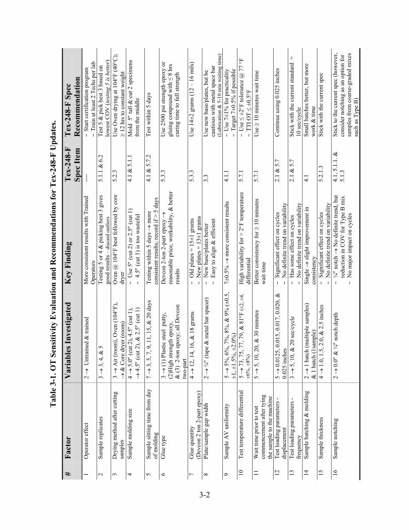
variability in the test results. Table 3-1 summarizes these variables together with the key findings

and proposed recommendations to the Tex-248-F specification. The proposed updates to the

Tex-28-F specification are included in the accompanying CD.

Detailed results and corresponding analysis of the Table 3-1 sensitivity evaluation are

documented in Report 0-6607-1 (Walubita et al., 2012). However, variables such as sample

thickness variation, load variations, sample notching, operator effect, etc., which were not

included in Report 0-6607-1 (Walubita et al., 2012) are discussed in the subsequent text. The

statistical threshold for all the analyses in this report is a COV of 30 percent

(Walubita et al., 2012). To exclude the aging effects and ensure usage of the same batch, a

different sets of samples were molded and tested each time the factors/variables were changed.

3-2

Tab

le 3

-1. O

T S

ensi

tivity

Eva

luat

ion

and

Rec

omm

enda

tions

for

Tex

-248

-F U

pdat

es.

# Fa

ctor

V

aria

bles

Inve

stig

ated

K

ey F

indi

ng

Tex

-248

-F

Spec

Item

T

ex-2

48-F

Spe

c R

ecom

men

datio

n 1

Ope

rato

r effe

ct

2 →

Unt

rain

ed &

trai

ned

Mor

e co

nsis

tent

resu

lts w

ith T

rain

ed

Ope

rato

rs

----

−

Star

t cer

tific

atio

n pr

ogra

m

− Tr

ain

at le

ast 2

Tec

hs p

er la

b 2

Sam

ple

repl

icat

es

3 →

3, 4

, & 5

Te

stin

g 5

or 4

& p

icki

ng b

est 3

giv

es

good

resu

lts –

dis

card

out

liers

5.

1.1

& 6

.2

Test

5 &

pic

k be

st 3

bas

ed o

n lo

wes

t CO

V (t

estin

g 5

is be

tter)

3

Dry

ing

met

hod

afte

r cut

ting

sam

ples

3 →

Air

(roo

m),

Ove

n (1

04°F

),

→ &

Cor

e dr

yer (

room

) O

ven

@ 1

04°F

bes

t fol

low

ed b

y co

re

drye

r 5.

2.3

Use

Ove

n dr

ying

at 1

04°F

(40°

C);

≥ 12

hrs

to c

onst

ant w

eigh

t 4

Sam

ple

mol

ding

size

4 →

5.0″ (

cut 2

), 4.

5″ (c

ut 1

),

→ 4

.5″

(cut

2),

& 2

.5″

(cut

1)

− U

se 5″

(cut

2) o

r 2.5″

(cut

1)

− 4.

5″ (c

ut 1

) is t

oo w

aste

ful

4.1

& 5

.1.1

M

old

5″

tall

& c

ut 2

spec

imen

s fro

m th

e m

iddl

e

5 Sa

mpl

e si

tting

tim

e fro

m d

ay

of m

oldi

ng

7 →

3, 5

, 7, 9

, 11,

15,

& 2

0 da

ys

Test

ing

with

in 5

day

s → m

ore

cons

iste

nt re

sults

; rec

ord

if >

5 da

ys

4.1

& 5

.7.2

Te

st w

ithin

5 d

ays

6 G

lue

type

3 →

(1) P

last

ic st

eel

putty

, (2

)Hig

h st

reng

th e

poxy

, &

(3)

2-to

n ep

oxy;

all

Dev

con

tw

o-pa

rt

Dev

con

2-to

n 2-

part

epox

y →

re

ason

able

pric

e, w

orka

bilit

y, &

bet

ter

resu

lts

5.3.

3 U

se 2

500

psi s

treng

th e

poxy

or

glui

ng c

ompo

und

with

≤ 8

hrs

cu

ring

time

to fu

ll st

reng

th

7 G

lue

quan

tity

(D

evco

n 2

ton

2-pa

rt ep

oxy)

4 →

12,

14,

16,

& 1

8 gr

ams

− O

ld p

late

s = 1

5±1

gram

s −

New

pla

tes =

13±

1 gr

ams

5.3.

3 U

se 1

4±2

gram

s (12

– 1

6 m

ils)

8 Pl

ate/

sam

ple

gap

wid

th

2 →

¼″

(tape

& m

etal

bar

spac

er)

− N

ew b

ase/

plat

es b

ette

r −

Easy

to a

lign

& e

ffici

ent

3.3

Use

new

bas

e/pl

ates

, but

be

caut

ious

with

met

al sp

ace

bar

(Lub

ricat

ion

& 5

-10

min

wai

ting

time)

9

Sam

ple

AV

uni

form

ity

5 →

5%

, 6%

, 7%

, 8%

, & 9

% (±

0.5,

±1

, ±1.

5%, ±

2.0%

) 7±

0.5%

→ m

ore

cons

iste

nt re

sults

4.

1.1

− U

se 7

±1%

for p

ract

ical

ity

− Ta

rget

7±0

.5%

if p

ossib

le

10

Test

tem

pera

ture

diff

eren

tial

5 →

73,

75,

77,

79,

& 8

1°F

(±2,

±4,

±6

%, ±

8%)

Hig

h va

riabi

lity

for >

2°F

tem

pera

ture

di

ffere

ntia

l 5.

7.1

− U

se ≤

±2°

F to

lera

nce

@ 7

7 °F

−

TTI O

T ≤

±0.5°F

11

W

ait t

ime

prio

r to

test

co

mm

ence

men

t afte

r tyi

ng

the

sam

ple

to th

e m

achi

ne

5 →

5, 1

0, 2

0, &

30

min

utes

B

ette

r con

sist

ency

for ≥

10

min

utes

w

ait t

ime

5.7.

1 U

se ≥

10

min

utes

wai

t tim

e

12

Test

load

ing

para

met

ers -

di

spla

cem

ent

5 →

0.0

125,

0.0

15, 0

.017

, 0.0

20, &

0.

025

inch

es

− Si

gnifi

cant

effe

ct o

n cy

cles

−

No

defin

ite tr

end

on v

aria

bilit

y 2.

1 &

5.7

C

ontin

ue u

sing

0.0

25 in

ches

13

Test

load

ing

para

met

ers -

fre

quen

cy

3 →

5, 1

0, &

20

sec/

cycl

e −

Has

som

e ef

fect

on

cycl

es

− N

o de

finite

tren

d on

var

iabi

lity

2.1

& 5

.7

Stic

k w

ith th

e cu

rren

t sta

ndar

d =

10

sec/

cycl

e 14

Sa

mpl

e ba

tchi

ng &

mol

ding

2 →

1 b

atch

(mul

tiple

sam

ples

)

& 1

bat

ch (1

sam

ple)

Si

ngle

→ sl

ight

impr

ovem

ent i

n co

nsis

tenc

y

4.1

Smal

l bat

ches

bet

ter,

but m

ore

wor

k &

tim

e 15

Sa

mpl

e th

ickn

ess

4 →

1.0

, 1.5

, 2.0

, & 2

.5 in

ches

−

Sign

ifica

nt e

ffect

on

cycl

es

− N

o de

finite

tren

d on

var

iabi

lity

5.2.

1.3

Stic

k w

ith th

e cu

rren

t spe

c

16

Sam

ple

notc

hing

2 →

0.0″ &

¼″ n

otch

dep

th

− ¼″ n

otch

→ N

o de

finite

tren

d, b

ut

redu

ctio

n in

CO

V fo

r Typ

e B

mix

−

No

maj

or im

pact

on

cycl

es

4.1,

5.1

.1. &

5.

1.3

Stic

k to

the

curr

ent s

pec

(how

ever

, co

nsid

er n

otch

ing

as a

n op

tion

for

sam

ples

from

coa

rse-

grad

ed m

ixes

su

ch a

s Typ

e B

)

3-3

Effects of OT Sample Thickness Variation

Three HMA mixes were evaluated and the sample thickness was varied from 1.0 to

2.5 inches. The standard OT test parameters were utilized, namely 0.025 inches displacement at a

loading frequency of 10 sec/cycle and a test temperature of 77°F. For each mix and sample

thickness, the research team molded and tested five replicate samples. Table 3-2 shows the

average results based on the best three (lowest COV).

Table 3-2. OT Sample Thickness Variation Results.

Thickness (Inches) Avg OT Cycles (Best 3 of 5) Type B with Limestone

Type C with Limestone RAP + RAS

Type D with Quartzite + RAP

1.0 - - 67 1.5 28 9 304 2.0 237 347 1,000+ 2.5 1,000+ 970 - Thickness (Inches) Statistical Variability (COV ≤ 30%) 1.0 - - 23% 1.5 22% 12% 11% 2.0 19% 18% - 2.5 - 16% -

In Table 3-2, the NMAS (refer to Table 2-1) and the marginal OT performance at

1.5 inch sample thickness did not warrant the need to evaluate the 1.0-inch thickness for the

Type B and C mixes. Therefore, only the Type D mix was evaluated at 1.0-inch thickness. From

the results in Table 3-2, the following two key points are evident:

• As theoretically expected, the laboratory OT cracking performance of the mixes

significantly improved with increasing sample thickness, i.e., the number of OT

cycles to failure rose almost exponentially with an increase in the sample thickness.

• There is no consistency or definitive trend in terms of the impact of the sample

thickness on variability as measured in terms of the COV. Therefore, varying the

sample thickness, while obviously improving the laboratory cracking performance

(i.e., number of cycles to failure), may not necessarily reduce variability in the test

results.

3-4

Effects of OT Load Variations – Displacement and Frequency

For this task, both the loading displacement and frequency were varied (minimum three

levels each) while the sample thickness was maintained at 1.5 inches. The displacement was

varied from 0.0125 to 0.025 inches, all applied at a loading frequency of 10 sec/cycle and a test

temperature of 77°F. Note that 0.025 inches is the currently specified OT loading displacement

based on the Tex-248-F test procedure (TxDOT, 2011); see Appendix A for comparisons with

some field data.

In the second part of the task, the loading frequency was varied from 5 to 20 sec/cycle

while maintaining the displacement and test temperature at 0.025 inches and 77°F, respectively.

Samples from the same batch for each mix type were specifically molded and tested for this task.

Figures 3-1 and 3-2 show these results (for up three HMA mixes).

Figure 3-1. Effects of Displacement Variations at Constant Frequency – 10 Sec/Cycle.

58; COV = 24%

150; COV = 25%

1007; COV = 18%

3; COV =5%

31; COV =15%

475; COV = 32%

25; COV= 28%

93; COV= 26%

962; COV= 31%

1

10

100

1,000

10,000

0.005 0.010 0.015 0.020 0.025 0.030

OT

Cycl

es

Displacement (Inches)

Type C (4.3%PG 76-22 + Limestone)

Type C (4.9%PG 70-22 + Limestone + 20%RAP)

Type B (4.6% PG 64-22 + Limestone + 30%RAP)

3-5

Since this task entailed reducing the displacement as well as varying the loading

frequency, only marginally performing mixes at 0.025 inches were selected for evaluation,

namely the Type B and C mixes. For the three HMA mixes evaluated, it is clear from Figure 3-1

that the following inferences can be made:

• There is a significant impact on the OT cycles with decreasing displacement, i.e., the

OT cycles are increasing as the displacement magnitude is decreased.

• There is no definitive trend or consistent effect on variability in terms of the COV.

This means that reducing the displacement while obviously increasing the number of

OT cycles may not necessarily reduce variability in the test results.

• As shown in Figure 3-2, changing the loading frequency at 0.025 inches constant

displacement, while having some effects on the number of OT cycles, offers little

benefit in terms of optimizing repeatability and minimizing variability in the test

results. Therefore, the current Tex-248-F specification of 0.025 inches and 10 sec/cycle

should be maintained.

Figure 3-2. Loading Frequency Variations at Constant Displacement – 0.025 Inches.

3; COV= 17%3; COV= 5%

7; COV=17%

21; COV= 27%

25; COV= 28%

30; COV= 32%

0

5

10

15

20

25

30

35

0 5 10 15 20 25

OT

Cycle

s

Loading Frequency (sec/cycle)

Type C (4.9% PG 70-22 +Limestone+ 20%RAP)

Type B (4.6% PG 64-22 + Limestone + 30%RAP)

3-6

Effects of Sample Notching

Three mixes were evaluated for this task; with ¼-inch notching (by ⅛-inch width) versus

zero notching. The standard Tex-248-F sample thickness of 1.5 inches was utilized. The

notching process took at least 45 minutes additional time. Different from the preceding tasks,

different samples, but coming from the same batch per mix type, were specifically molded and

tested for this particular task. Figure 3-3 shows the results of this sensitivity task based on the

best three replicate samples out of a total of five.

Figure 3-3. Effects of Sample Notching on the OT Results.

As shown in Figure 3-3, the sample notching measuring ¼-inch (depth) by ⅛-inch

(width) had the following effects on the three mixes that were evaluated:

• There is no significant impact on the number of OT cycles to failure, i.e., the number

of OT cycles were insignificantly different when comparing the notched to the

un-notched sample results.

• There is no definitive trend or significant impact on variability in terms of the COV

for the dense-graded Type C mixes. Although not shown in Figure 3-3, a similar trend

was also observed for the fine-graded mixes.

¼″ notch depth by 1/8 ″ width(∼ 45 minutes additional process)

No notch

28%

17%

28%

12%

26%

23%

0%

5%

10%

15%

20%

25%

30%

Type B (4.6% PG 64-22 + Limestone + 30%RAP) Type C (5.0% PG 64-22 + 20%RAP ) Type C (5.0% PG 70-22+ 16% RAP + 3%RAS)

Varia

bility

(COV

)

0.00" Notch 0.25" Notch

25Cycles

47 Cycles

31Cycles

3-7

• However, a significant decrease in the COV was noted for the coarse-graded Type B

mix. While the average number of OT cycles were hardly different, the COV for the

notched samples was over half that of the un-notched samples, i.e., 12 percent

(notched) versus 28 percent.

Therefore, recommendations are to stick to the current practice of not notching the

1.5-inch thick samples. However, notching should be considered an option for samples from

coarse-graded mixes such as Type B to improve consistency.

OT Crack Failure Mode

Theoretically, single cracking is the desired failure mode for HMA samples subjected to

OT testing. In practice however, this is not often the case. Multiple cracking will often (but not

always) occur in some samples, particularly for the coarse-graded mixes. Examples of both

single and multiple cracking are shown in Figure 3-4.

Figure 3-4. Single and Multiple Cracking in Some OT Samples.

Single crack

Multiple cracks

3-8

As can be noted in Figure 3-4, aggregate size and orientation are the predominant factors

contributing to the occurrence of multiple cracking, with the coarse-graded mixes being more

vulnerable. Multiple cracking particularly occurs when a big rock is in the direction of the crack

and the crack (s) has to go around the rock. When multiple cracking occurs, the samples will

typically sustain higher number of OT cycles than its counterpart samples with single cracks. In

addition to an increase in the OT cycles, there will also be high variability in the overall test

results.

Based on the aforementioned observations in Figure 3-4 and for the mixes evaluated in

this study, the following can be concluded:

• Multiple cracking will often (but not always) occur, particularly in coarse-graded

mixes – predominantly when a big rock is in the direction of the crack.

• Compared to fine- or dense-graded mixes, coarse-graded mixes because of their

aggregate size and orientation are more prone to multiple cracking under OT testing.

Therefore, the occurrence of high variability in the coarse-grade mixes such as Type B

should also not be unexpected when testing these coarse-graded mixes in the OT.

• As per part of the Tex-248-F modification recommendations, the number of cracks

occurring on OT test specimens should be recorded and reported as part of the OT

test results.

• However, where there is an opportunity to re-mold more samples or the best three

results (COV ≤30%) can be obtained from the tested pool of 5 sample replicates, then

it is recommended to simply discard all the samples with multiple cracks.

Alternative OT Data Analysis Methods

As a supplement to just reporting the number of OT cycles to failure, various alternative

approaches to analyzing the OT test data were investigated. Table 3-3 summarizes the results of

these investigations. Report 0-6607-1 (Walubita et al., 2012) documents the detailed discussions

of these methods along with the analyses.

3-9

Table 3-3. Alternative OT Data Analysis Methods (Walubita et al., 2012).

# Method Variables Investigated Key Findings and Recommendations

1 Load reduction criterion 50, 75, 85, & 93% load drop − 50 & 75% – Not viable, sharp drop in load with small & hardly differentiable OT cycles

− 85% load drop gives reasonable COV with interpretable OT cycles, but still requires validation & correlation with field data

2 Rate of load decrease Slope change in the load-cycle response curve

Unsatisfactory results. The inflexion point could not be determined beyond 50% load drop.

3 Pseudo fracture energy (Pseudo-FE)

Area under the load-cycle response curve

No improvement in variability with the use of Pseudo-FE

4 OT monotonic testing and fracture parameters

Tensile strength (σt), failure strain (εt), fracture energy (FE), and FE Index

The FE Index exhibited promising potential and is discussed in details in Chapter 4.

Of the four approaches evaluated in Table 3-3, only the FE Index measured and

computed from the OT monotonic testing exhibited promising potential. Note that as opposed to

the classical tensile strength, failure strain, and fracture energy (FE), the FE Index is a new HMA

fracture parameter derived in the course of this study. Chapter 4 discusses this FE Index in

greater detail.

OT ROUND-ROBIN TESTING AND OPERATOR EFFECT

Following the Tex-248-F specification recommendations in Table 3-1, the research team

conducted parallel and round-robin testing between TTI and three TxDOT laboratories. Prior to

starting these tests, the team checked and calibrated all the OT machines in each laboratory; see

examples in Appendices A and B.

As a minimum, each laboratory was tasked to test the same three mixes with five

replicate samples per HMA mix type per variable evaluated. Table 3-4 through 3-8 shows the

results based on an average of the best three replicates (out of a total of five replicates)

considering the lowest COV. Note that a statistical Excel® macro was developed and is available

to automatically pick the best three results out of a total of four or five replicates. As indicated in

Table 3-1, outliers should be discarded—only the best three results with the lowest COV should

be reported.

3-10

Table 3-4. OT Round-Robin Results – Laredo Type C Mix.

Laredo Type C Mix = 5% PG 64-22 + Gravel + 1% Lime + 20% RAP Sample ID# TxDOT Lab

(Austin) TxDOT Lab (Childress)

TxDOT Lab (Houston)

TTI Lab (Lubinda)

TTI Lab (Hossain)

OT1 54 41 72 43 46

OT2 38 53 73 36 41

OT3 52 37 52 32 71

Avg 48 44 66 37 55

COV (≤ 30%) 18% 19% 18% 15% 26%

Results considering all 5 OT replicate samples

Avg 60 51 50 43 79

COV 29% 59% 47% 29% 54%

Table 3-5. OT Round-Robin Results – Four Different HMA Mixes.

HMA Mix TxDOT Lab (Austin)

TxDOT Lab (Childress)

TxDOT Lab (Houston)

TTI Lab (CS)

Chico Type D (4.5% AC) - 119 - 118

Laredo Type C (+ 20% RAP) 48 44 66 46

Waco Type C (+16% RAP & 3% RAS)

- 25 37 38

Atlanta Type D (+20% RAP) 389 410 354 304

Statistical Variability (COV ≤ 30%)

Chico Type D (4.5% AC) - 9% - 12%

Laredo Type C (+20% RAP) 18% 19% 18% 27%

Waco Type C (+16%RAP & 3% RAS)

- 34% 10% 30%

Atlanta Type D (+20% RAP) 29% 12% 31% 11%

3-11

Table 3-6. OT Operator Effect.

Sample ID# TTI – Hossain (Trained)

TTI – Unnamed (Untrained)

TTI – Lubinda (Self-Trained)

OT1 150 180 250

OT2 242 458 186

OT3 239 143 196

Avg 210 260 211

COV (≤ 30%) 25% 66% 16%

Results considering all 5 OT replicate samples

Avg 175 348 247

COV 39% 108% 31%

Table 3-7. Trained Operator Effect.

Type D = 5.0% PG 70-22 + Limestone Operator Year of

Testing Location Avg OT

Cycles COV Comment

Lubinda 2009 Round-robin

TTI, TxDOT labs, & PaveTex

258 23% 28 replicate samples in total were molded & tested; 1 sample cut from 2.5″

Lubinda 2011 (June) TxDOT-CST 213 17% Best 3 out of 5; 2 samples cut from 5.0″

Hossain 2011 (June) TTI 230 27% Best 3 out of 5; 2 samples cut from 5.0″

Hossain 2011 (June) TTI 210 25% Best 3 out of 5; 1 sample cut from 4.5″ (New base & plates)

Jason 2012 (July) TTI 197 23% Best 3 out of 5; 2 samples cut from 5.0″

Jacob 2012 (Aug) TTI 211 16% Best 3 out of 5; 2 samples cut from 5.0″

3-12

Table 3-8. Trained Operator and Equipment Effect.

Type D = 5.1% PG 64-22 + Quartzite + 20% RAP

AV (7±1%) OT Cycles

Operator Hossain (Trained)

Lubinda (self-trained)

Hossain (Trained)

Lubinda (Self-trained)

OT equipment & location TTI TxDOT – Austin

OT1 6.8% 7.1% 309 294

OT2 6.1% 6.6% 121 241

OT3 6.4%` 6.5% 334 197

OT4 6.3% 6.4% 269 257

OT5 6.6% 6.9% 240 306

Avg (all) 6.4% 6.7% 255 259

COV (all) 4.3% 4.4% 32.6% 17%

Results – Best 3 out of 5

Avg (best 3) 6.4% 6.5% 304 286

COV (best 3) (≤ 30%) 2.4% 1.5% 11% 9%

In general, Tables 3-4 through 3-8 show reasonable and acceptably promising results in

terms of variability, with most of the COV values being less than 30 percent. As theoretically

expected, variability was generally higher for the coarse-graded, RAP, and RAS mixes compared

to the fine- and dense-graded mixes; but still within the COV tolerance limit. Therefore, high

variability in these mixes (i.e., coarse-graded, RAP, RAS, etc.) should not be completely

unexpected when subjected to the OT testing in repeated loading mode.

Overall, the results shown in Table 3-4 through 3-8 suggest that the OT repeatability can

be optimized and variability minimized if the following actions are considered:

• The Tex-248-F updates and modifications as suggested in Table 3-1 should be

adhered to. Based on these recommendations, TxDOT is strongly encouraged to

implement these updates and modifications as itemized in Table 3-1. A CD is also

included to provide a step-by-step video demo of these new updates and suggested

changes.

3-13

• The OT machines should be periodically checked and calibrated for both load and

displacement measurements. This aspect is discussed in the subsequent sections of

this chapter.

• All technicians and operators running the OT machines must be trained and certified.

For starters, at least two technicians/operators must be trained per lab and a

certification program initiated. This OT certification program can either be an online

course along with video demos or following the format of the TxDOT standard

certification training programs.

OT SOFTWARE, CALIBRATION, AND MAINTENANCE

As discussed in the subsequent text, an effort was also made to address the following OT

machine operational aspects (in liaison with ShedWorks):

• Harmonization and upgrading of the OT software.

• Development of a new OT calibration kit/software.

• Development of OT calibration and service maintenance manuals; see the included

CD.

OT Software Updates

To ensure software consistency, an OT software upgrade (Version 1.9.0) was installed on

two TTI and TxDOT-Austin machines with the assistance of ShedWorks. Childress and Houston

District labs are next in line. New features accompanying the OT Version 1.9.0 software include

the following:

• The Start button is disabled when the machine pump is off.

• A time delay function has being installed. With this function, the operator can input

the desired sample relaxation or temperature conditioning time prior to testing, i.e.,

prior to applying load to the sample.

• The software has been reprogrammed to terminate only and only if five load peaks in

a consecutive row are below the specified threshold. This feature eliminates the

occurrence of premature test termination due to sudden drops or spikes in the load,

which was a problem with the previous software versions.

3-14

To verify the operational status of the new software (Version 1.9.0), verification testing

was conducted on one TTI machine using HMA mixes of known OT results from the previous

version of the software, on the same OT machine. Following the recommendations in Table 3-1

and picking the best three replicate results out of a total of five, Table 3-9 shows that there is a

slight improvement in terms of optimizing repeatability and minimizing variability for the

dense-graded Type C and D mixes that were tested. For the same OT machine, the COV values

based on the new software (Version 1.9.0) are comparatively lower than those based on the older

software version.

Table 3-9. OT Results – New (Version 1.9.0) versus Old Software.

HMA Mix Old Software

New Software (Version 1.9.0)

Comment

Type D = 5.5% PG 64-22 + Limestone

AVG OT cycles = 822 769 Significant decrease in COV

COV = 31.30% 1.03% Type C = 4.8% PG 70-22 + 20% RAP

AVG OT cycles = 9 8 About 37.5% decrease in COV

COV = 12.29% 7.53% Type B with RAP (Coarse-graded)

AVG OT cycles = 25 39 COV insignificantly different & high – typical of coarse-graded mixes COV = 28.00% 31.20%

OT Calibration – Load and Displacement

As part of the OT software upgrade, ShedWorks also developed and supplied a new

calibration kit along with the associated software. Figure 3-5 shows that the key feature of this

new calibration kit is its ability to automatically measure and record both load and displacement

data while simultaneously displaying linear graphical plots on the screen. The recorded data can

then be used for later analyses as needed.

3-15

Figure 3-5. The New OT Calibration Kit and Examples of Linear Graphical Screen Plots.

Unlike the old kit that was not automated and did not record any data or directly measure

displacements, this new calibration kit shows potential towards optimizing the operational

accuracy of the OT machines. The OT calibration procedure and steps are documented in the OT

Calibration Manual, which is included in the accompanying CD. A video demo of the calibration

process is also included in the CD.

The key recommendations based on the calibrations that were conducted on the TTI OT

machines include the following:

• If possible, the OT Calibration Manual should be an integral part of or be used in

conjunction with the Tex-248-F specification.

• The calibrations should be performed semi-annually and whenever needed (i.e., when

abnormalities are observed in the machine and/or results).

• Both the load and displacement tolerances should not exceed ±5 percent when and

after performing the calibrations. Otherwise, the OT Calibration Manual should be

referenced to address this aspect.

• The typical load and displacement calibration curves should be linear; see the

example in Figure 3-6 for the load-voltage curve for a well-calibrated OT load cell.

3-16

• It is also recommended to verify both the calibrations and control tuning with dummy

trial testing (minimum three samples) or using synthetic samples and thereafter,

checking the raw data files as shown in Figure 3-7. During verification of the raw

data files, the initial load prior to start of testing should not exceed ±10 lb while the

displacement should be within the ±5 percent tolerance limit; otherwise the OT

machine should be recalibrated or checked for control tuning. Details of these aspects

can be found in the OT Calibration Manual in the CD accompanying this report.

Figure 3-6. Typical Load-Voltage Response Curve – Well-Calibrated OT Load Cell.

3-17

Figure 3-7. OT Verification of the Raw Data Files.

OT Service Maintenance

Routinely checking and servicing the OT machine is one way to optimize its operational

accuracy and longevity. As part of this study, the researchers developed the OT Service

Maintenance Manual, a draft copy of which is included in the accompanying CD of this report.

Based on the observations of this study and as detailed in the OT Service Maintenance Manual,

the key aspects associated with the OT service maintenance should include the following:

• If possible, the OT Service Maintenance Manual should be an integral part of or be

used in conjunction with the Tex-248-F specification.

• Perform routine service maintenance on a yearly basis and whenever needed,

i.e., when abnormalities are observed in the machine and/or results.

• Check the hydraulic, mechanical, and electrical components.

• Check for oil leaks, dust, etc.

3-18

SUMMARY

While taking due cognizance of the fact that repeated loading crack tests are by their

nature inherently associated with high variability (particularly for coarse-graded, RAP, and RAS

mixes) and that the OT is no exception, the work presented in this chapter shows promise to

optimize the OT repeatability and minimize variability in the test results. With this in mind, the

key findings and recommendations derived from this chapter are summarized as follows:

• The recommended Tex-248-F updates and modifications should be implemented.

• A training and certification program should be initiated for all the technicians and

operators that will be running the OT machines. As a minimum, two

technicians/operators should be trained and certified per laboratory.

• For consistency and software harmonization, the new updated OT software

(Version 1.9.0) should be installed on all the TTI and TxDOT OT machines.

• OT calibrations and service maintenance should be routinely performed

semi-annually and yearly, respectively; and whenever needed, i.e., when

abnormalities are observed in the machine and/or test results.

• If OT calibration and control tuning verification are needed, dummy samples

(minimum three) or synthetic samples should be used for this purpose.

• The calibration and service manuals along with the video demo should accompany

the modified Tex-248-F specification.

• A Round-robin must be conducted once the new software (Version 1.9.0) has been

installed on all the OT machines and they have all been calibrated using the new

calibration kit.

• Since ShedWorks is going out of business, the team recommends that TxDOT and/or

TTI consider purchasing and evaluating one of the OT machines that other suppliers

are currently manufacturing.

4-1

CHAPTER 4: THE OT TEST METHOD – DYNAMIC AND MONOTONIC LOADING MODES

In an attempt to identify a surrogate crack test to be routinely used to evaluate HMA

cracking resistance potential in the laboratory, the researchers explored the Overlay Tester (OT)

test in a monotonic loading mode in addition to the more commonly used repeated (dynamic)

loading mode. For easy identification, the following abbreviations, “OTR” and “OTM” are used

to denote the “Repeated (dynamic)” and “Monotonic” loading OT tests, respectively. This

chapter discusses and compares the test setups and test results for both of these tests.

TEST SETUP

The same test setup is used for both the monotonic loading and repeated loading OT tests.

In the repeated loading test, the ram moves back and forth horizontally to apply the loading

cycles (Tex-248-F); for the monotonic loading OT, the ram movement is unidirectional.

Figure 4-1 presents the overlay test setup and the loading configurations. Table 4-1 lists and

compares the key aspects of the two test methods; subsequent sections discuss these aspects in

further details.

Table 4-1. OTM and OTR Test Parameters.

OTM OTR (Tex-248-F)

Test configuration

Sample dimensions 6″ L × 3″ W × 1.5″ T 6″ L × 3″ W × 1.5″ T

Loading mode Monotonic tension displacement controlled

Repeated tension displacement controlled

Test parameters

Loading rate = 0.125 inch/min Temperature = 77°F

Frequency = 10 sec/cycle (or 0.1 Hz) (5 sec loading + 5 sec unloading)

Loading rate = 0.025 inches displacement Temperature = 77°F

Output data Strength ( tσ ), Strain ( tε ), Stiffness

( tE ), FE ( fG ), & FE Index Number of load repetitions (cycles) to failure &

peak load

Test time per specimen ≤ 10 minutes ≤ 180 minutes

4-2

Figure 4-1. Overlay Tester (OT) Setup.

The Monotonic OT (OTM) Test Method

The OT is a simple performance test traditionally used for characterizing the reflective

cracking resistance potential of HMA mixes in the laboratory under repeated loading (tension)

mode (Zhou et al., 2007). It is an electro-hydraulic system that applies direct tension load to

specimens.

The key components of the OT device, as shown schematically in Figure 4-2, consist of

two steel plates, one fixed and the other able to move horizontally to simulate the opening and

closing of joints or cracks in the old pavements beneath an overlay. The specimen is spanned

across the opening and epoxied to the horizontal surface platens with half of the length of the

Loading Configuration

Pictorial Setup

Specimen Dimension

150 mm

38 mm

76 mm

4-3

specimen resting on each platen. The OT test specimens are 6 inches long, 3 inches wide and

1.5 inches thick (Figure 4-1); which can either be laboratory molded, cut from field cores, or

fabricated from field sawn slabs (Walubita et al., 2011). Based on the Texas standards, the

laboratory molded test specimens for most conventional Texas HMA mixes are typically

fabricated to a total final air voids (AV) content of 7 ± 1 percent (Zhou and Scullion, 2005).

As demonstrated in this study, the OT test setup was also run in monotonic loading mode

to supplement the standard repeated loading OT test (Tex-248-F) (Walubita et al., 2012). That is

the specimen was tested within the OT test setup in a controlled displacement mode where the

monotonic loading rate and test temperature can be suitably selected or changed as desired. For

this study, the monotonic loading rate was 0.125 inch/min and the test temperature was 77°F,

with a minimum pre-conditioning time of two hours (Walubita et al., 2011). This temperature

was monitored via a thermocouple probe attached inside a dummy HMA specimen also placed in

the same OT temperature chamber as the test specimens. At 0.125 inch/min loading rate, the total

test time was no more than 10 minutes. With temperature pre-conditioning of the test specimens

conducted in a separate chamber, over 20 HMA specimens can easily be tested within a day.

The Repeated OT (OTR) Test Method

The overall test setup is the same for a repeated loading and a monotonic loading OT test

with the ram direction and loading rates being the only significant difference. For the OTR test,

the setup is programmed to move the ram back and forth horizontally at a much faster loading

rate than its monotonic counterpart. Each loading cycle lasts for 10 seconds with 5 seconds

loading and 5 seconds unloading with a maximum horizontal displacement of 0.025 inches until

crack failure occurs. The specimen dimensions for the standard OTR test are the same as those

for the OTM test. Details of the OT test procedure can be found in the TxDOT test specification

Tex-248-F (TxDOT, 2011).

4-4

TEST RESPONSE CURVES AND DATA ANALYSIS

This section discusses the output data from the two test methods and their subsequent

data analysis models.

The OTM Data Analysis Models

During OT monotonic loading testing, the measurable parameters include the applied

load, the horizontal tensile displacement rate, time, and the test temperature. The primary output

of the OT monotonic loading test is the stress-strain response curve of the HMA mix. Figure 4-2

illustrates a typical OT monotonic loading test output data.

Figure 4-2. Load-Displacement Response Curve: OTM Testing.

The fracture parameters measured from the OTM tests in this study include the HMA

tensile strength ( tσ ), HMA tensile strain at peak failure load or ductility potential ( tε ), HMA

tensile modulus or stiffness in tension ( tE ), HMA fracture energy or FE ( fG ), and the fracture

energy index or FE Index. The tensile strength is determined according to the standard models of

mechanics as the ratio of the peak failure load and the specimen x-sectional area as follows:

maxσ =t

Ptb

4-1

Loa

d, f

(w)

Displacement, w

Pmax

DPmaxDo

4-5

where t and b are the thickness and the width of the specimen respectively, and maxP is the

axial peak load (see Figure 4-2). The tensile strain at peak load or the ductility potential is

measured as:

max.@.@

P ot

o

Disp pick load D DInitial disp zero load D

ε −= =

4-2

where maxPD and oD are the displacement at peak load and initial displacements, respectively

(Figure 4-2). The ratio of the tensile strength and the tensile strain is denoted as the tensile

modulus or the stiffness in tension.

tt

t

HMAtensile strengthETensile strain

σε

= = 4-3

The fracture energy is defined as the work required to produce a crack of unit surface

area, measured in J/m2. The work required to fracture the sample is represented by the area under

the load versus displacement curve (see Figure 4-2). Therefore, a general expression for Fracture

Energy can be written as:

( )1

fWorkG f x dx

Area of cracked section A= = ∫ 4-4

Finally, the fracture energy index is defined as a parametric ratio of the fracture energy to

the HMA tensile strength and tensile strain at peak failure load per unit crack length.

31 10 εσ

= × ft

cr t

GFE Index

l 4-5

where crl is the length traversed by the crack (the specimen thickness t , in case of the OTM test).

Note that the parameters tσ , tε , tE , and FE ( fG ) [i.e., Equations 4-1 through 4-4] are the

traditional HMA fracture parameters typically measured and computed from most monotonic

crack tests. The FE Index, on the other hand, is a new HMA fracture parameter derived in the

course of this study.

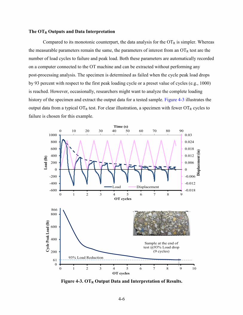
4-6

The OTR Outputs and Data Interpretation Compared to its monotonic counterpart, the data analysis for the OTR is simpler. Whereas

the measurable parameters remain the same, the parameters of interest from an OTR test are the

number of load cycles to failure and peak load. Both these parameters are automatically recorded

on a computer connected to the OT machine and can be extracted without performing any

post-processing analysis. The specimen is determined as failed when the cycle peak load drops

by 93 percent with respect to the first peak loading cycle or a preset value of cycles (e.g., 1000)

is reached. However, occasionally, researchers might want to analyze the complete loading

history of the specimen and extract the output data for a tested sample. Figure 4-3 illustrates the

output data from a typical OTR test. For clear illustration, a specimen with fewer OTR cycles to

failure is chosen for this example.

Figure 4-3. OTR Output Data and Interpretation of Results.

0 10 20 30 40 50 60 70 80 90

-0.018

-0.012

-0.006

0

0.006

0.012

0.018

0.024

0.03

-600

-400

-200

0

200

400

600

800

1000

0 1 2 3 4 5 6 7 8 9

Time (s)

Disp

lace

men

t (in

)

Load

(lb)

OT cycles

Load Displacement

0

200

400

600

800

0 1 2 3 4 5 6 7 8 9 10

Cycle

Pea

k Lo

ad (l

b)

OT cycles

93% Load Reduction

866

61

Sample at the end of test @93% Load drop

(9 cycles)

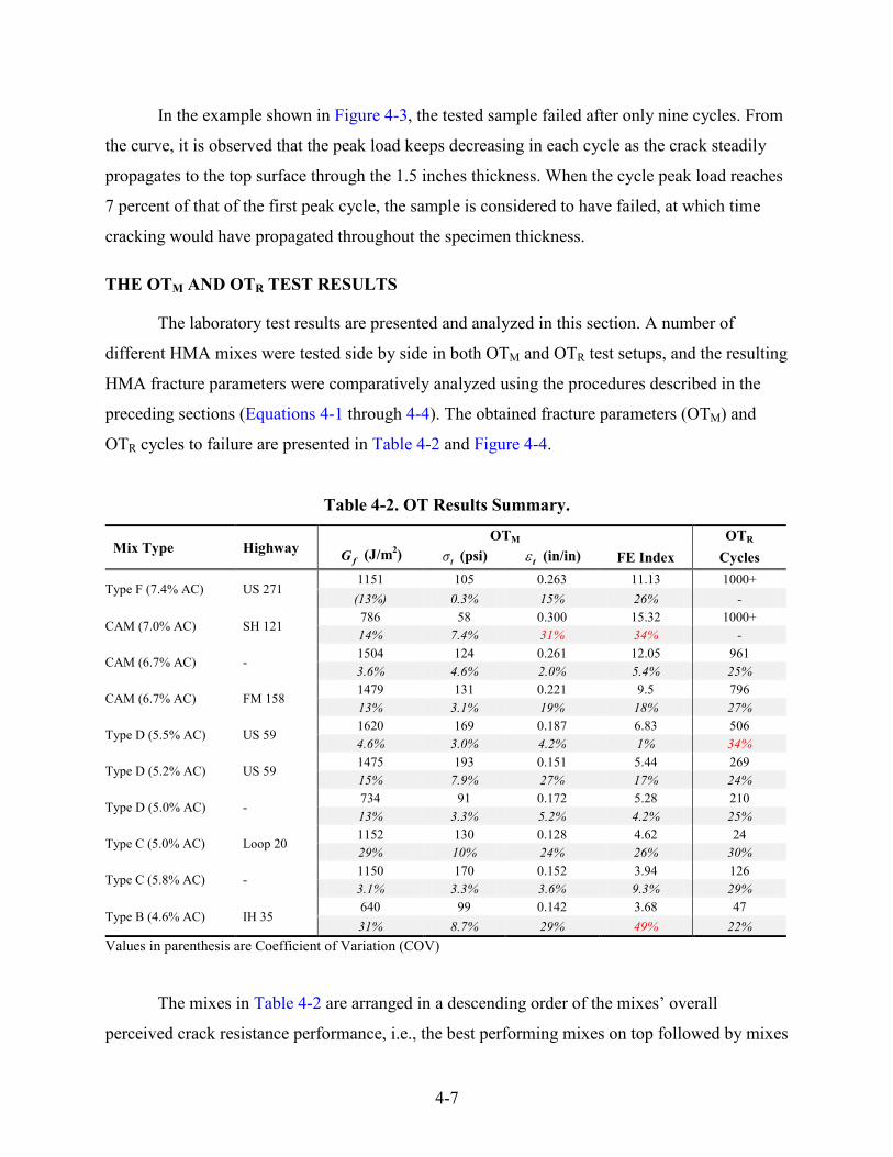
4-7

In the example shown in Figure 4-3, the tested sample failed after only nine cycles. From

the curve, it is observed that the peak load keeps decreasing in each cycle as the crack steadily

propagates to the top surface through the 1.5 inches thickness. When the cycle peak load reaches

7 percent of that of the first peak cycle, the sample is considered to have failed, at which time

cracking would have propagated throughout the specimen thickness.

THE OTM AND OTR TEST RESULTS

The laboratory test results are presented and analyzed in this section. A number of

different HMA mixes were tested side by side in both OTM and OTR test setups, and the resulting

HMA fracture parameters were comparatively analyzed using the procedures described in the

preceding sections (Equations 4-1 through 4-4). The obtained fracture parameters (OTM) and

OTR cycles to failure are presented in Table 4-2 and Figure 4-4.

Table 4-2. OT Results Summary.

Mix Type Highway OTM OTR

fG (J/m2) tσ (psi) tε (in/in) FE Index Cycles

Type F (7.4% AC) US 271 1151 105 0.263 11.13 1000+

(13%) 0.3% 15% 26% -

CAM (7.0% AC) SH 121 786 58 0.300 15.32 1000+ 14% 7.4% 31% 34% -

CAM (6.7% AC) - 1504 124 0.261 12.05 961 3.6% 4.6% 2.0% 5.4% 25%

CAM (6.7% AC) FM 158 1479 131 0.221 9.5 796 13% 3.1% 19% 18% 27%

Type D (5.5% AC) US 59 1620 169 0.187 6.83 506 4.6% 3.0% 4.2% 1% 34%

Type D (5.2% AC) US 59 1475 193 0.151 5.44 269 15% 7.9% 27% 17% 24%

Type D (5.0% AC) - 734 91 0.172 5.28 210 13% 3.3% 5.2% 4.2% 25%

Type C (5.0% AC) Loop 20 1152 130 0.128 4.62 24 29% 10% 24% 26% 30%

Type C (5.8% AC) - 1150 170 0.152 3.94 126 3.1% 3.3% 3.6% 9.3% 29%

Type B (4.6% AC) IH 35 640 99 0.142 3.68 47 31% 8.7% 29% 49% 22%

Values in parenthesis are Coefficient of Variation (COV)

The mixes in Table 4-2 are arranged in a descending order of the mixes’ overall

perceived crack resistance performance, i.e., the best performing mixes on top followed by mixes

4-8

with relatively poor performances, for easy comparison. This perception of the mix cracking

performance is based on their historical field and laboratory performance. The primary

assessment of the results presented in Table 4-2 suggests that among the four fracture parameters

calculated from the OTM test, only the FE Index values correlates to the perceived performance

of their corresponding mixes and the OTR cycles, whereas the fracture energy, tensile strength,

and tensile strain parameters show no justifiable trend. On the other hand and as shown in

Figure 4-4, the repeated OT cycles to failure very closely follow the order of mixes, which is

further evidence to the well-established correlation of the OTR with the field performances of the

HMA mixes.

Figure 4-4. Comparison of HMA Mixes Based on OTM and OTR Test Results.

However, the failure of the OTM fracture parameters, other than the FE Index, to reflect

the mixes’ perceived performances is not completely unexpected. The tensile strength (function

of the peak load) and the strain (function of displacement at the peak load) only takes the load

increment portion of the load-displacement response curve into account (Figure 4-2). On the

other hand, the fracture energy (function of the area under the load-displacement curve), while

considering the complete loading history of the specimen, fails to effectively capture the mixes’

behavior due to the compensating effects of increasing and decreasing areas under the response

786

15041151

1479 1620 1475

734

1152 1150

640

15.3212.05 11.13

9.56.83 5.44 5.28 4.62 3.94 3.68

1000 961 1000796

506269 210

24126 47

0

500

1000

1500

2000 0

5

10

15

200

300

600

900

1200

CAM CAM Type F CAM Type D Type D Type D Type C Type C Type B7.0% AC 6.7% AC 7.4% AC 6.7% AC 5.5% AC 5.2% AC 5.0% AC 5.0% AC 5.8% AC 4.6% AC

Fracture Energy FE Index OT Cycles

OT

Cyc

les

FE In

dex

FE (J

/m2 ) Mon

oton

icO

TR

epea

ted

OT

Mix Types

4-9

curves (Figure 4-2) (Walubita et al., 2012). The FE Index effectively combines these three

fracture parameters to capture the complete loading history of the specimen so that it can show a

better reflection of the expected cracking performance of the mix. This is also clearly presented

in Figure 4-4, where the FE Index exhibits a clear trend from the best performing CAM mix to

the least crack-resistant Type B mix. Consequently, the FE Index parameter has a clear

correlation with the OTR cycles to failure. To further investigate this correlation, the OTR cycles

to failure for the tested mixes were plotted against their corresponding FE Index values from

OTM test and are presented in Figure 4-5.

Figure 4-5. Relationship between the OTR Cycles and OTM FE Index.

Data shown in Figure 4-5 provide evidence of a linear relationship between the values of

OT cycles (from repeated loading OT test) and FE Index (from monotonic loading OT test), with

a coefficient of correlation (R2) of 96.5 percent. Inevitably, Figure 4-5 suggests that there is

promising potential in using the FE Index as a surrogate and/or supplementary screening

parameter to the OT cycles. In addition, this analysis provided a correlation model to estimate

the OT cycles to failure based on its FE Index measured from the monotonic loading OT test.

The general form of this correlation equation is:

( )= × −OT Cycles A FE Index B 4-6

where the parameters A and B are determined using simple linear curve fitting of the data in

Figure 4-5. Theoretically, this correlation would imply that the number of OT cycles can be

y = 121.36x - 404.74R² = 0.9654

0

200

400

600

800

1000

1200

0 4 8 12 16

Cyc

les t

o fa

ilure

(OT

R)

FE Index (OTM)

CAM

Type F

Type D

Type C

Type B

4-10

estimated based on the FE Index computed from the much simpler and shorter monotonic

loading OT test. Note that by comparison, the monotonic loading OT test is a practically much

shorter test to run than the repeated loading OT test—an average of 5 to 10 minutes test time

(monotonic loading OT) versus a test time range of 30 minutes to as much as over 3 hours

(repeated loading OT), depending on the HMA mix type. However, results from more HMA

mixes need to be considered and analyzed to calibrate this regression function (Equation 4-6),

before it can be reliably used as a means to correlate the two parameters.

Screening of HMA Mixes: Discriminatory Ratios and Statistical Analysis

One important aspect to consider for the HMA cracking tests is their ability to perform as

HMA mix screeners, which is crucial in the HMA mix-design process. Already based on the

results presented in Table 4-2 and Figure 4-4, an assessment of the potential of the evaluated

fracture parameters to differentiate the crack resistance potential of the mixes is obtained. To

further investigate the ability of the fracture parameters to screen mixes, two approaches were

used: the discriminatory ratio (DR) concept and Tukey’s HSD statistical analysis.

The discriminatory ratio (DR) is an arithmetic ratio of two corresponding parametric

values (e.g., fG , tσ , FE Index, and OTR Cycles) comparing a good mix with a relatively poor

mix. The larger the DR in magnitude, the greater the difference between the mixes and the more

effective the fracture parameter is in discriminating and differentiating the mixes. To compare

the DR-based mix screening ability of the fracture parameters, researchers intuitively chose three

mixes, namely the CAM (7.0 percent AC) designated as ‘very good’ (VG) mix, the Type D

(5.2 percent AC) as a ‘good’ (G) mix, and the Type B (4.6 percent AC) as a ‘poor’ (P) mix.

Table 4-3 presents the resulting DR values.

Table 4-3. Screening of HMA Mixes Based on Discriminatory Ratios.

Mix Type OTM OTR

fG σ t ε t FE Index Cycles CAM/Type B 1.23 0.59 2.11 4.16 21.28 CAM/Type D 0.53 0.30 1.99 2.82 3.72 Type D/Type B 2.30 1.95 1.06 1.48 5.72

Based on the DR values computed in Table 4-3, it is evident that the OTR cycles to failure

provides a significantly superior degree of discrimination between any pair of mixes than the

4-11

facture parameters from OTM test. Among the OTM fracture parameters, only the FE Index

shows acceptable discrimination between the mixes, though not nearly as prominent as the OTR

cycles.

Analysis of variance (ANOVA) and Tukey’s Honestly Significant Differences (HSD)

multiple comparison procedure at a 95 percent confidence level were also used to statistically

investigate the potential of the test parameters’ ability to differentiate the crack resistance

potential of the HMA mixes. The interpretation of the ANOVA results in Table 4-4 is as follows:

for a particular test method; the mixes having parametric values that are statistically not

significantly different are listed in the same group (e.g., A, B, or C). A mix categorized in

Group A has higher numerical values than a mix listed in Group B for the same parameter and

the difference in their numeric values are statistically significant. For example in the last column

of Table 4-4, the Type F and the CAM mixes has the highest OTR cycles and hence, are

categorized in Group A, whereas the Type B and Type C mixes fall in the same group (Group

C), which indicates that the difference in their OTR cycles is statistically insignificant. The OTR

cycles for Type D mixes fall in between these two groups and are categorized in the same group

(Group B), which also signifies that their respective values are not significantly different from

each other.

Table 4-4. Screening of HMA Mixes Based on ANOVA and Tukey’s HSD Analysis.

Mix Type Highway OTM OTR

fG (J/m2) tσ (psi) tε (in/in) FE Index Cycles Type F (7.4% AC) US 271 A B A A A CAM (7.0% AC) SH 121 B C A A A CAM (6.7% AC) - A B A A A CAM (6.7% AC) FM 158 A B A A A Type D (5.5% AC) US 59 A A B B B Type D (5.2% AC) US 59 A A B B B Type D (5.0% AC) - B B B B B Type C (5.0% AC) Loop 20 A B B B C Type C (5.8% AC) - A A B B C Type B (4.6% AC) IH 35 B B B B C

Before discussing the significance of the results presented in Table 4-4, it is important to

note that, while comparing two mixes based on a certain parametric value, the Tukey’s HSD

method of statistical analysis takes their respective result variability into account. Therefore, any

fracture parameter that has a high degree of result variability (high COV) is less likely to show

any statistical discrimination among mixes. Therefore, despite showing good discrimination

4-12

among mixes based on the DR values (Table 4-2), in the statistical analysis, the FE Index

parameter, due to relatively high results variability, does not show effectiveness in categorizing

mixes. As expected, the fracture energy and the tensile strength parameters categorized the mixes

in a totally random fashion. However, the mix categorization based on the tensile strain and that

based on the FE Index are identical.

Sensitivity to Change in Mix Design Parameters

A Type D mix (PG 70-22 + Limestone) with three different AC levels (4.5, 5.0, and

5.5 percent) was utilized to assess the sensitivity of the two test methods to HMA mix-design

variables such as AC variations. Table 4-5 and Figure 4-6 present the computed facture

parameters.

Table 4-5. Sensitivity to AC Variations.

AC OTM OTR

fG (J/m2) σ t (psi) ε t (mm/mm) FE Index Cycles 4.5% 728 (3.0%) 107 (8.2%) 0.132 (13%) 3.4 (3.4%) 165 (6.6%) 5.0% 734 (13%) 91 (3.3%) 0.172 (5.2%) 5.28 (4.2%) 210 (25%) 5.5% 826 (7.8%) 72 (4.6%) 0.264 (12%) 11.51 (10%) 822 (31%)

Values in parenthesis are Coefficient of Variation (COV)

Figure 4-6. OTM and OTR Test Parameter Sensitivity to AC Variation.

3.405.28

11.51

728 734 826

0

50

100

150

165 210

822

0

4

8

12 0

300

600

900

0

300

600

900

10791 72

4.5% 5.0% 5.5%

Asphalt Binder Content

Tens

ileSt

reng

th

(psi)

FE In

dex

FE (J

/m2 )

Cyc

les

OT R

OT M

4-13

The results in Table 4-5 and Figure 4-6 show that among the OTM fracture parameters

assessed, the FE Index is the most sensitive to AC change. Theoretically, cracking resistance

potential of mixes should show an increasing trend with increasing asphalt binder content since,

at higher binder contents, mixes become softer and more ductile. This is reflected in the

increasing trend that the FE Index and OTR cycles show. Also, decreasing tensile strength with

increasing asphalt content is an expected trend, since at higher binder contents the mix gets softer

and fails at a lower peak load. The fracture energy values, on the other hand, did not show any

significant differences for 4.5 percent and 5.0 percent AC levels.

To further investigate the sensitivity of the OTM fracture parameters to asphalt binder

content change, discriminatory ratios were evaluated and are presented in Table 4-6 along with

the results from the ANOVA and Tukey’s HSD statistical analysis.

Table 4-6. Sensitivity to AC: Discriminatory Ratios and Statistical Analysis.

Analysis Type AC

OTM OTR

fG σ t ε t FE Index Cycles

Discriminatory Ratio (DR)

5.5%/4.5% 1.13 0.79 1.53 3.39 4.98 5.5%/5.0% 1.13 0.67 2.00 2.18 3.91 5.0%/4.5% 0.99 1.18 0.77 1.55 1.27

Statistical (ANOVA & Tukey’s HSD)

4.5% A A B C B 5.0% A B B B B 5.5% A C A A A

From the results in Table 4-6, the sensitivity of the fracture parameters of the two test

methods are clearly evident. Both the FE Index and the OTR cycles parameters show satisfactory

sensitivity when DR values are considered. However, it is more evident in case of the statistical

analysis, particularly the FE Index that discriminates the three AC levels in the theoretically

expected order, i.e., 5.5 percent AC categorized in the group A followed by 5.0 percent AC in

group B and finally 4.5 percent AC in group C. However, the OTR cycles are not as efficient in

categorizing the different AC levels in appropriate groups primarily due to their high variability

in the test results.

4-14

To further investigate the sensitivity of the OT (both monotonic and repeated loading),

another Type D mix (PG 64-22 + Quartzite +20 percent RAP) was tested by varying the asphalt

binder content between 5.2 percent and 6.2 percent; Table 4-7 presents the results.

Table 4-7. AC Sensitivity: Type D Mix.

Mix Parameter 5.2% AC 5.6% AC 6.2% AC

Atlanta Type D: PG 64-22 + Quartzite + 20% RAP

OTM

FE Index (Monotonic) 5.44 6.28 7.13

OT cycles (Repeated) 269 469 655

Table 4-7 bears further evidence that both the monotonic loading and the repeated

loading OT tests are sensitive to asphalt binder content change. Often it is important for a test

procedure to be able to differentiate among specimens tested at different temperatures.

Therefore, a Type C mix was tested in the OTM and the OTR test setups to evaluate the sensitivity

to temperature variations. The results are presented in Table 4-8.

Table 4-8. Temperature Sensitivity of the OTM and the OTR Tests.

Mix Parameter 50°F 59°F 77°F

Laredo Type C: PG 64-22 + Crushed Gravel + 20% RAP + 1% Lime

OTM

FE Index (Monotonic) 0.66 0.70 1.93

OTR cycles (Repeated) 2 3 25

From the above table, it is evident that both the OTR and the OTM tests are sensitive to

temperature variation with the repeated loading mode showing significantly higher sensitivity.

However, at low temperatures, the mixes get much more brittle resulting in lower crack

resistance and Type C being a relatively poor crack-resistant mix somewhat magnifies this effect

for specimens tested at lower temperatures.

COMPARISON OF THE OTM AND OTR TEST METHODS

Based on the results presented in the preceding sections and the subsequent discussions,

Table 4-9 compares the characteristic attributes of the two test methods.

4-15

Table 4-9. Comparison of OTM and OTR Test Methods.

Category OTM OTR

Sample preparation Easy Easy

Potential to test field cores Yes Yes

Overall test simplicity Very simple Very simple

Test time per specimen ≤ 10 minutes ≤ 180 minutes

Test variability at 77°F (COV ≤ 30%) Repeatable Reasonable if the recommendations

in Chapter 3 are adhered to!

Mix screening ability Good Very Good

Sensitivity to AC variations Good Very good

Correlation to field data Needs validation Yes

Practicality of implementation Yes Yes

From the overall comparison of the two test methods, it is observed that both tests have

promising potential to be routinely used as HMA fracture tests. The repeated OT ranks above the

monotonic OT when correlation to field data and mix screening capabilities are considered; on

the other hand, the OTM is a faster, cost-effective test with better repeatability. However, the

potential correlation between these two test methods based on the FE Index (OTM) and number

of cycles (OTR) is a promising avenue for further studies that can lead to the establishment of a

more complete HMA routine crack test.

SUMMARY

This chapter provided a comparative exploration of two of the prospective routine HMA

crack test methods, namely the monotonic loading overlay tester (OTM) test and the repeated

loading overlay tester (OTR) test using the same OT equipment setup. From the overall findings

of this study, these researchers recommend both tests as having promising potential as HMA

routine crack tests using the same equipment setup, with the OTR ranking ahead of the OTM.

Therefore, the OTM can serve as a supplement and/or surrogate to the current OTR Tex-248-F,

which is easily implementable since the two test methods use the same equipment setup.

5-1

CHAPTER 5: THE IDT AND R-IDT TEST METHODS

In view of developing test procedures for surrogate HMA cracking tests, the indirect

tension test was explored in repeated loading mode (R-IDT) as well as the more traditional

monotonic loading mode (IDT). This chapter presents the testing setups and obtained results.

TEST SETUP

Table 5-1 lists and compares the key aspects of the two test methods, which are discussed

in further detail in the subsequent sections of this chapter.

Table 5-1. IDT and R-IDT Test Parameters.

IDT R-IDT

Test configuration

Sample dimensions 6″φ × 2.5″ T 6″φ × 2.5″ T

Loading mode Monotonic compressive

Repeated compressive (load/stress controlled)

Test parameters

Loading rate = 2.0 inch/min Temperature = 77°F

Frequency = 1 Hz (0.5 sec loading + 0.5 sec rest) Input load = 25% of the averaged IDT peak loads of all mixes evaluated in study (630 lb for all mixes)

Contact load = 5% of input load for all mixes) Temperature = 77°F

Output data Strength ( tσ ), Strain ( tε ), Stiffness

( tE ), FE ( fG ), & FE Index Number of load repetitions (cycles) to failure

& cycle index

Test time per specimen ≤ 10 minutes ≤ 180 minutes

Legend: L = length; W = width; T = thickness, H = height; φ = diameter

5-2

The Indirect Tension (IDT) Test

Indirect-tension testing is more of more traditional monotonic crack test used to

characterize the fracture properties of HMA mixes in the laboratory (TxDOT, 2004, Walubita et

al., 2002). The typical IDT setup requires a servo-hydraulic closed-loop testing machine capable of

axial compression (Huang et al., 2005). Several publications recommend using a loading rate of

2 inches/min; most notably are the standard procedures in Tex-226-F (TxDOT, 2004) and ASTM

D6931 (ASTM, 2005). Typical IDT specimens are 6 inches in diameter and 2.5 inches thick

(TxDOT, 2004).

The specimen is typically loaded diametrically in compression and this indirectly induces

horizontal tensile stresses in the middle zone of the specimen that ultimately causes cracking. For

the evaluation of the tensile properties of HMA, the permanent deformation under the loading

strip is undesirable (Huang et al., 2005). Therefore, the compressive load is distributed using

loading strips, which are curved at the interface to fit the radius of curvature of the specimen.

The strain at the center of the specimen is determined from the horizontal displacements

measured using Linear Variable Displacement Transducers (LVDTs) with 2-inch gauge length.

However, one issue that may be problematic with the IDT set-up is the gauge length of the

LVDTs. The existence of large aggregates, particularly for coarse-graded mixes, in the middle of

the specimen can affect the displacement measurements between gauge points if the length is too

short. So, caution must be exercised to watch out for such potential problems and account for

them in the subsequent data analyses and interpretation of the results.

However, to address the complicacies associated with the measurement of horizontal

displacement using LVDTs, particularly in the case of test practicality and industry applications,

these researchers have established correlation models to predict the horizontal displacement from

the vertical RAM displacement for different mixes. Three specimens were tested for each mix

type, namely Type D, Type B, Type C, and CAM, and the horizontal displacements recorded

from the LVDTs were plotted against the vertical RAM displacement (Figure 5-1). Curve fitting

techniques were then applied to generate correlation models for each mix types; as shown in

Figure 5-1. Corresponding Excel macros were also developed to automatically calculate the

horizontal displacements from the vertical RAM displacements so the operators would not have

to worry about LVDTs.

5-3

Figure 5-1. IDT Horizontal Displacement Calculation from Vertical (Ram) Displacements.

For consistency with the OT tests, the specimens were tested at 77°F. The data captured

during IDT testing include time, applied load, and horizontal and vertical specimen deformation.

The Repeated Loading Indirect Tension (R-IDT) Test

Preliminary repeated IDT loading tests were also conducted to investigate their R-IDT

suitability and practicality for characterizing the HMA mix cracking resistance potential in the

lab. With the R-IDT test method, the cracking resistance potential of a mix is characterized by

the number of IDT load repetitions to crack failure. While the IDT test is a fairly established

HMA testing procedure, its use as a repeated loading test is a novel approach. Therefore, no

standard specification was found for this test method. The only literature reference was found in

Walubita et al. (2010) and was used as the primary basis towards establishing the testing

procedures. A tentative test loading parameter set was established after several trial testing

sessions and is summarized in this section.

The same specimen dimension as the regular IDT test (6 inches diameter × 2.5 inches

thick) is used for its repeated R-IDT counterpart. The test is a two-point loading setup in a

y = -3.2379x3 + 1.0866x2 + 0.0674xR² = 0.9999

y = -4.5575x3 + 1.4935x2 + 0.0263xR² = 0.9998

y = -1.3804x3 + 0.9154x2 + 0.0195xR² = 0.9995

y = -3.4597x3 + 1.273x2 + 0.0988xR² = 1

0.000

0.005

0.010

0.015

0.020

0.025

0.030

0.035

0.040

0.00 0.03 0.06 0.09 0.12 0.15

LV

DT

dis

plac

emen

t (in

)

Ram Displacement (in)

Type D

Type B

Type C

CAM

5-4

load-controlled mode, which is the primary difference of the R-IDT with the repeated OT test

that is a displacement controlled test. The reason for running this test in a load-controlled mode

instead of a displacement controlled mode is that the sample configuration and loading setup to

run these tests in displacement-controlled mode is very complex. The repeated loading mode is

established by loading the specimen at a frequency of 1 Hz with 0.5 seconds of loading followed

by 0.5 seconds of rest. Twenty-five percent of the average IDT peak load of all the mixes in this

study was selected as the R-IDT input load (i.e., 630 lb in this study for all mixes) and 5 percent

of the input load was selected as the contact load (i.e., rounded off to 30 lb for all mixes in this

study) (Walubita et al., 2010). Consistent with the OT and IDT tests, the R-IDT tests were also

conducted at room temperature (77°F). In summary, the test conditions, test parameters, and

input loads were the same for all the mixes evaluated under the R-IDT test in this study.

Permanent deformation at the points of loading in both the IDT and R-IDT tests may

undesirably occur at test temperatures such as 77°F or higher, leading to a possible composition

of both compressive and tensile failure modes in the specimen with multiple cracks (Molenaar et

al., 2002). This was not accounted for in this study. However, the temperature used for these tests

(i.e., 77°F) was chosen for consistency of comparison with the OT tests, i.e., the OTR based on the

Tex-248-F specification (TxDOT, 2009) is required to be performed at 77°F. Therefore, all other

tests were performed at the same temperature. This temperature also facilitates use in industry

procedures, since 77°F is considered room temperature.

TEST RESPONSE CURVES AND DATA ANALYSIS MODELS

The output data from the two tests and their subsequent data analysis models are

discussed in this section.

The IDT Data Analysis Models

Typically the result of interest from an IDT test is the axial peak load, which is analyzed

using established models to calculate the HMA tensile strength. However, the full potential of

the IDT as a HMA cracking test is utilized when the complete loading history of a sample is

taken into consideration by analyzing the full load-displacement response. Figure 5-2 shows a

typical load-displacement response from an IDT test. Several fracture parameters in addition to

the HMA tensile strength are calculated from this output response curve.

5-5

Figure 5-2. Load-Displacement Response Curve: IDT Testing.

The typical fracture parameters measured from the IDT tests in this study include the

HMA tensile strength ( tσ ), HMA tensile strain at peak failure load or ductility potential ( tε ),

HMA tensile modulus or stiffness in tension ( tE ), and HMA fracture energy or FE ( fG ). There

are several models for calculating the tensile strength available in the literature. For this study,

the model that Huang et al. (2005) proposed was used assuming plane stress conditions:

max2

tPtD

σπ

= 5-1

where t and D are the thickness and the diameter of the specimen respectively, and maxP is the

axial peak load, as indicated in Figure 5-2. The tensile strain at peak load or the ductility

potential is calculated as follows:

max.@.@

P ot

o

Disp pick load D DInitial disp zero load D

ε −= =

5-2

where maxPD and oD are the displacement at peak load and initial displacements, respectively

(Figure 5-2). The ratio of the tensile strength and the tensile strain is denoted as the tensile

modulus or the stiffness in tension.

tt

t

HMAtensile strengthETensile strain

σε

= =

5-3

5-6

The fracture energy is defined as the work required to produce a crack of unit surface

area, measured in J/m2. The work required to fracture the sample is represented by the area under

the load versus displacement curve, as shown in Figure 5-2. Therefore, a general expression for

Fracture Energy can be written as:

( )1

fWorkG f x dx

Area of cracked section A= = ∫ 5-4

Finally, the fracture energy index (FE Index), which is a new parameter derived in this

study, is defined as a parametric ratio of the fracture energy to the HMA tensile strength and

tensile strain at peak failure load per unit crack length. This FE Index was computed as follows:

51 10 ft

cr t

GFE Index

lε

σ= × 5-5

where crl is the length traversed by the crack.

The R-IDT Test Outputs and Data Analysis Models

The primary output response parameters from the R-IDT test are the displacement,

cycles, and time count. Figure 5-3 shows a plot of the input load and the resulting displacement

outputs for a typical R-IDT test. For clarity, only the first eight cycles were presented.

Figure 5-3. R-IDT Load (Input) – Displacement (Output) Curve.

0 2 4 6 8

0

200

400

600

800

0

0.02

0.04

0.06

0.08

0.1

0 2 4 6 8Cycles

Load

(lb)

Disp

lace

men

t (in

)

Time (sec)

Displacement Load

5-7

Figure 5-4 presents cycle peak displacements plotted against R-IDT cycles to

demonstrate the selection of failure cycles. The notations S#1, S#2, and S#3 refer to sample #1,

sample #2, and sample #3, respectively.

Figure 5-4. Evolution of Peak Displacement with the Number of Load Cycles.

In addition to the number of load cycles and to account for the load-controlled mode of

the R-IDT test method, the data analysis from these tests included the Cycle Index concept

(Equation 5-6). The Cycle Index was introduced to provide a baseline comparison with the OTR

results that are based on displacement controlled loading mode and was computed as follows:

1 Input LoadCycle Index Cycles Sitting Load

−= ×

5-6

In the above equation, Cycles corresponds to the number of R-IDT load cycles to crack

failure as illustrated in Figure 5-4. The input and sitting load were 630 lb and 30 lb, respectively

for all mixe, as defined in the previous section and illustrated in Figure 5-3. Like the number of

cycles in the OTR test, the higher the Cycle Index in magnitude, the better the HMA mix in terms

of crack resistance potential.

IDT AND R-IDT TEST RESULTS

The laboratory test results for the IDT and the R-IDT tests are presented and analyzed in

this section, including test method comparisons and sensitivity to AC variations.

438 519 5680.0

0.2

0.4

0.6

0.8

0 100 200 300 400 500 600

Cyc

le P

eak

Disp

. (in

)

Number of Cycles

R-IDT-S#1

R-IDT-S#2

R-IDT-S#3

5-8

IDT Test Results: Comparison of HMA Mixes

Like in Chapter 4 for the OT, the same three mixes were tested, namely a Type B mix

from Waco District, a Type D mix from Atlanta District, and a CAM mix from Paris District.

The details mix designs for each of these three mixes are discussed in Chapter 2. Figure 5-5

presents the IDT test results for the three mixes.

Figure 5-5. IDT Test Outputs: Load-Displacement Response Curves.

From the above figure, it is evident that the IDT test properly reflected the expected

behavior of these three mixes. The CAM, usually known for being a softer and more

crack-resistant mix, have the most ductile response curve with low peak load, whereas the

Type B mix shows much more brittle response behavior. The Type D is clearly a better mix than

Type B both in terms of higher peak load and ductility potential.

Equations 5-1 through 5-5 were used on the generated load displacement response data to

calculate the fracture parameters. Table 5-2 and Figure 5-6 present the results.

0

500

1000

1500

2000

2500

3000

3500

0 0.05 0.1 0.15 0.2

Loa

d (lb

-f)

Displacement (in)

Type B

Type D

CAM

Before Test After Test

5-9

Table 5-2. Summary of IDT Test Results.

Mix Type Fracture Energy, fG Tensile Strength, tσ Strain, tε

FE Index (J/m2) (lb-in/in2) (psi) (MPa) (mm/mm)

Type B 136(2.3%) 0.779(2.3%) 103(3.8%) 0.710(3.8%) 0.0149(9.9%) 1.88(11.8%)

Type D 193(8.1%) 1.101(8.1%) 127(3.7%) 0.876(3.7%) 0.0190(19.4%) 2.76(24.4%)

CAM 226(5.2%) 1.290(5.2%) 79(2.0%) 0.547(2.0%) 0.0340(4.1%) 9.21(10.0%)

* Values in parenthesis are the Coefficient of Variance (COV).

Based on the COV values, the test seem to be very repeatable with all the COV values

within the acceptable limit (≤30 percent). The computed parametric values also seem to be

reasonable and are consistent with literature publications. For instance, the IDT tensile strength

values are indifferent from the 85~200 psi Texas specification (TxDOT, 2004).

Figure 5-6. Summary of IDT Test Results.

From the computed fracture parameters in Table 5-2 and Figure 5-6, it is clear that the

tensile and strain parameters are not very reflective of the mixes’ perceived laboratory cracking

resistance performance. The tensile strength (function of the peak load) and the strain (function

1.88 2.76

9.21

0

4

8

12 100

150

200

2500

50

100

150

136

193

226

103127

79

Type B Type D CAM

Ten

sile

Stre

ngth

(psi)

FE In

dex

Frac

ture

Ene

rgy

(J/m

2 )

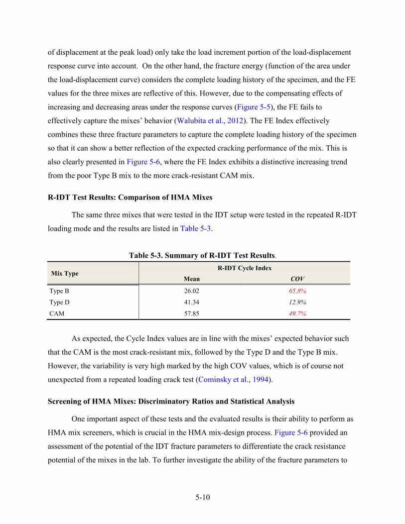
5-10

of displacement at the peak load) only take the load increment portion of the load-displacement

response curve into account. On the other hand, the fracture energy (function of the area under

the load-displacement curve) considers the complete loading history of the specimen, and the FE

values for the three mixes are reflective of this. However, due to the compensating effects of

increasing and decreasing areas under the response curves (Figure 5-5), the FE fails to

effectively capture the mixes’ behavior (Walubita et al., 2012). The FE Index effectively

combines these three fracture parameters to capture the complete loading history of the specimen

so that it can show a better reflection of the expected cracking performance of the mix. This is

also clearly presented in Figure 5-6, where the FE Index exhibits a distinctive increasing trend

from the poor Type B mix to the more crack-resistant CAM mix.

R-IDT Test Results: Comparison of HMA Mixes

The same three mixes that were tested in the IDT setup were tested in the repeated R-IDT

loading mode and the results are listed in Table 5-3.

Table 5-3. Summary of R-IDT Test Results.

Mix Type R-IDT Cycle Index

Mean COV

Type B 26.02 65.8%

Type D 41.34 12.9%

CAM 57.85 49.7%

As expected, the Cycle Index values are in line with the mixes’ expected behavior such

that the CAM is the most crack-resistant mix, followed by the Type D and the Type B mix.

However, the variability is very high marked by the high COV values, which is of course not

unexpected from a repeated loading crack test (Cominsky et al., 1994).

Screening of HMA Mixes: Discriminatory Ratios and Statistical Analysis

One important aspect of these tests and the evaluated results is their ability to perform as

HMA mix screeners, which is crucial in the HMA mix-design process. Figure 5-6 provided an

assessment of the potential of the IDT fracture parameters to differentiate the crack resistance

potential of the mixes in the lab. To further investigate the ability of the fracture parameters to

5-11

screen mixes, the researchers used two approaches: the discriminatory ratio (DR) concept and

Tukey’s HSD statistical analysis.

The discriminatory ratio is an arithmetic ratio of two corresponding parametric values

(e.g., fG , tσ , FE Index, and Cycle Index) comparing a good mix with a relatively poor mix. The

larger the DR in magnitude, the greater the difference between the mixes and the more effective

the fracture parameter is in discriminating mixes. Based on the DR values computed in Table 5-4,

it is evident that the IDT FE Index provides a superior degree of discrimination between good and

poor lab crack-resistant mixes than the other facture parameters. The R-IDT Cycle Index is also

able to differentiate the mixes, but is not as pronounced when compared to the differentiating

ability of the OT cycles of the OTR test (Table 4-3).

Table 5-4. Screening of HMA Mixes Based on Discriminatory Ratios.

Mix Type IDT R-IDT

fG σ t ε t FE Index Cycle Index

CAM/Type B 1.66 0.77 2.28 4.90 2.22

CAM/Type D 1.17 0.62 1.79 3.34 1.40

Type D/Type B 1.42 1.23 1.28 1.47 1.59

Analysis of variance (ANOVA) and Tukey’s Honestly Significant Differences (HSD)

multiple comparison procedure at a 95 percent confidence level were used to statistically

investigate the potential of the test parameters’ ability to differentiate the crack resistance

potential of the HMA mixes. The interpretation of the ANOVA results in Table 5-5 is as follows:

for a particular test method, the mixes having parametric values that are statistically not

significantly different are listed in the same group (e.g., A or B). A mix categorized in Group A

has higher numerical values than a mix listed in Group B for the same parameter and the

difference in their numeric values are statistically significant. For example in the FE Index

column of Table 5-5, the CAM mix has the highest IDT FE Index value and hence is categorized

in Group A. Type B and Type D fall in the same group (Group B), which indicates that the

difference in their FE Index values is statistically insignificant.

5-12

Table 5-5. Screening of HMA Mixes Based on ANOVA and Tukey’s HSD Analysis.

Mix Type IDT R-IDT

fG (J/m2) σ t (psi) ε t (mm/mm) FE Index Cycles Index Type B B A B B B Type D B A B B B CAM A B A A A

Following the results in Table 5-5, it is clear that both the IDT and R-IDT tests yield

similar categorization of the mixes based on the ANOVA and Tukey’s HSD statistical analysis.

Likewise, this analysis mostly fails to show any clear discrimination among Type D and Type B

mix types. However, one needs to consider that, while comparing two mixes based on a certain

parametric value, the Tukey’s HSD method of statistical analysis takes their respective result

variability into account. Therefore, any fracture parameter that has a high degree of result

variability (high COV) is less likely to show any statistical discrimination among mixes.

However, since only three mixes were evaluated, the research team recommends conducting

additional testing with more mixes to substantiate these findings.

Sensitivity to Change in Asphalt Binder Content

Similar to the OT in Chapter 4, a Type D mix (PG 70-22 + Limestone) with three

different AC levels (4.5, 5.0, and 5.5 percent) was utilized to assess the sensitivity of the tests to

HMA mix-design variables such as AC variations. The computed facture parameters are

presented in Table 5-6 and Figure 5-7. Values in parenthesis in Table 5-6 are Coefficient of

Variation (COV).

Table 5-6. Sensitivity to AC Variations.

AC IDT R-IDT

fG (J/m2) σ t (psi) ε t (mm/mm) FE Index Cycles Index 4.5% 114 (2.2%) 85 (3.1%) 0.0145 (1.4%) 1.84 (1.2%) 54.4 (28%) 5.0% 124 (4.7%) 75 (6.2%) 0.0179 (7.5%) 2.81 (4.6%) 59.8 (6.4%) 5.5% 203 (2.6%) 110 (3.9%) 0.0204 (6.9%) 3.59 (11%) 104.5 (18%)

5-13

Figure 5-7. IDT and R-IDT Test Parameter Sensitivity to AC Variation.

The results in Table 5-6 and Figure 5-7 show that both the IDT and the R-IDT tests are

capable of capturing the effect of AC variation. However, among the IDT fracture parameters,

FE Index is the most sensitive to AC change. Theoretically, the cracking resistance potential of

mixes should show an increasing trend with increasing asphalt binder content since, at higher

binder contents, mixes become softer and more ductile. This is reflected in the increasing trend

that the FE, FE Index, and Cycle Index parameters show. On the other hand, due to this

increased softness, mixes should fail at lower peak loads, resulting in lower tensile strengths.

However, the IDT tensile strength at 5.5 percent AC is higher than those at lower AC levels. The

reason behind this behavior is that at higher binder contents, the IDT loading strips sink into the

soft material at the contact surface, resulting in a failure mode that is both compressive and

tensile. At some instances, multiple crack paths might also develop, requiring higher peak loads

to failure. Therefore, caution must be exercised while applying the IDT and R-IDT test methods

at higher AC levels and softer mixes, particularly at test temperatures of 77°F or higher.

1.842.81

3.59

114 124203

0

50

100

15054.4 59.8

104.5

01234 0

100

200

300

0

50

100

150

85 75

110

4.5% 5.0% 5.5%

Asphalt Binder Content

Tens

ileSt

reng

th

(psi

)FE

Inde

x

FE (J

/m2 )

Cyc

le In

dex

R-ID

TID

T

5-14

To further investigate the sensitivity of the IDT and R-IDT fracture parameters to asphalt

binder content change, discriminatory ratios are evaluated and presented in Table 5-7 along with

the results from the ANOVA and Tukey’s HSD statistical analysis.

Table 5-7. Sensitivity to AC: Discriminatory Ratios and Statistical Analysis.

Analysis

Type AC IDT

fG σ t ε t FE Index Cycle Index

Discriminatory Ratio (DR)

5.5%/4.5% 1.78 1.29 1.41 1.95 1.92 5.5%/5.0% 1.64 1.47 1.14 1.28 1.75 5.0%/4.5% 1.09 0.88 1.23 1.53 1.10

Statistical (ANOVA & Tukey’s HSD)

4.5% B B B C B 5.0% B C A B B 5.5% A A A A A

From the results in Table 5-7, the sensitivity of the fracture parameters of the two tests

are clearly evident. Both the FE Index and the Cycle Index parameters show satisfactory

sensitivity when DR values are considered. However, it is more evident in case of the statistical

analysis. Specifically, the FE Index discriminates all three AC levels in the expected order, i.e.,

5.5 percent AC categorized in group A, followed by 5.0 percent AC in group B, and finally

4.5 percent AC in group C. However, the R-IDT cycles are not as efficient in categorizing the

different AC levels in the appropriate grouping due to their high result variability.

5-15

COMPARISON OF THE IDT AND R-IDT TEST METHODS

Based on the results presented in the preceding sections and the subsequent discussions, a

comparison between the two test methods is presented in Table 5-8.

Table 5-8. Comparison of IDT and R-IDT Test Methods.

Category IDT R-IDT

Sample preparation Very Easy Very Easy

Potential to test field cores Yes Yes

Overall test simplicity Very simple Fair

Test time per specimen ≤ 10 minutes ≤ 180 minutes

Test variability at 77°F (COV ≤ 30%) Repeatable Variable

Mix screening ability Moderate Moderate

Sensitivity to AC variations good Moderate

Correlation to field data N e e d s v a l i d a t i o n

Practicality of implementation Yes Possible

From the overall comparison of the two test methods, it is observed that both tests have

promising potential to be routinely used as a HMA fracture test. However, due to its overall test

simplicity, better repeatability, and slightly better mix screening ability, the IDT with shorter test

time along with the use of the FE Index will rank ahead of its repeated loading counterpart

(R-IDT) as a routine HMA crack test.

SUMMARY

This chapter provided a comparative exploration of two of the prospective surrogate

crack test methods, namely the indirect tension test (IDT) and the repeated loading indirect

tension test (R-IDT). From the overall findings of the study, the researchers recommend both

tests to have promising potential as HMA routine crack tests with the IDT ranking ahead of the

R-IDT test. However, caution and use of robust loading strips are strongly recommended,

particularly for high AC mixes and/or high temperature testing where applying the IDT and

R-IDT tests can be quite problematic.

6-1

CHAPTER 6: THE SCB AND R-SCB TEST METHODS

As the continuation of the search for an alternative HMA cracking test, the semicircular

bending test is evaluated in this chapter, both in the monotonic (SCB) and repeated (R-SCB)

loading modes.

TEST SETUP

Table 6-1 lists and compares the key aspects of the two test methods, which are then

discussed further in the subsequent sections of this chapter.

Table 6-1. SCB and R-SCB Test Parameters.

IDT R-SCB

Test configuration

Sample dimensions 6″φ × 3″ H × 2.5″ T (0.25″ notch) 6″φ × 3″ H × 2.5″ T (0.25″ notch)

Loading mode Monotonic compressive Repeated compressive (load/stress controlled)

Test parameters

Loading rate = 0.05 inch/min Temperature = 77°F

Frequency = 1 Hz (0.5sec loading + 0.5 sec rest) Input load = ~50% of the averaged SCB peak load of

all mixes studied (i.e., 175 lb for all mixes tested) Contact load = 5% of input load for all mixes

Temperature = 77°F

Output data Strength ( tσ ), Strain ( tε ), Stiffness

( tE ), FE ( fG ), & FE Index Number of load repetitions (cycles) to failure

& cycle index

Test time per specimen ≤ 10 minutes ≤ 180 minutes

Legend: L = length; W = width; T = thickness, H = height; φ = diameter

The Semi-Circular Bending (SCB) Test

Development of SCB as a predictor of HMA cracking resistance potential in the lab has

appeared relatively recent in the field of pavement engineering. The SCB specimen is a half disk,

typically 6 inches in diameter that is loaded in compression using a three-point flexural

apparatus. Different specimen thicknesses have been reported in the literature. However, to

maintain consistency with the other considered tests, the research group tested 2.5-inch thick

6-2

samples in this study. The rate at which the specimen is loaded is also not very well-specified,

but Walubita et al. (2002) have had success when using 0.05 in/min loading rate, and this was

rate used in this study.

Specimen fabrication and preparation for the SCB test is somewhat complicated due to

the notch in the base of the specimen. The notch ensures that the crack initiates at the center of

the specimen base. Notch depths vary, depending on many factors such as specimen thickness,

diameter, loading rate, test temperature, mix type, aggregate size, etc. Once again, the work of

Walubita et al. (2002) was taken as reference while selecting the notch depth of 0.25 inch.

At first glance, the calculation of stiffness in the middle point of the lower specimen

surface may seem difficult because affixing the strain gauges onto the specimen is time- and

resource-consuming. In the case of the current study, however, HMA stiffness determination was

an important parameter to explore. To accommodate this requirement, the research team

calculated the horizontal strain based on the vertical RAM displacements following the

procedures explained in Chapter 5 (Figure 5-1). Corresponding Excel macros were also

developed to automatically calculate the horizontal displacements from the vertical RAM

displacements so the operators would not have to worry about LVDTs.

For analysis purposes, the spacing between the supports is typically 0.8 times the

specimen diameter. From the literature search, the typical test temperatures for the SCB test are

between 50°F (Huang et al., 2009) and 77°F (Molenaar et al., 2002). To be consistent with the

other crack tests repeated in the previous chapters, the researchers selected 77°F as the test

temperature. The data captured during SCB testing include time, applied load, and horizontal and

vertical specimen deformation.

The Repeated Loading Semi-Circular Bending (R-SCB) Test

The research team conducted preliminary repeated SCB loading tests to investigate the

R-SCB suitability and practicality for characterizing the HMA mix cracking resistance. With the

R-SCB test method, the cracking resistance potential of a mix is characterized by the number of

SCB load repetitions to crack failure. Similar to the R-IDT test, the only literature reference was

found in Walubita et al. (2010) and was used as the primary basis towards establishing the

R-IDT testing procedures. A tentative test loading parameter set was established after several

trial testing and is summarized in this section.

6-3

The same specimen dimensions as the regular SCB test (6 inches diameter × 3 inches tall

× 2.5 inches thick) are used for its repeated R-SCB counterpart. The test involved a three-point

dynamic compressive loading that induces tension at the bottom zone of the semicircular

specimen. Similar to the R-IDT, the R-SCB is run in a load-controlled mode because the sample

configuration and loading setup to run this test in displacement-controlled mode is very complex.

The repeated loading mode is established by loading the specimen at a frequency of 1 Hz with

0.5 seconds of loading followed by 0.5 seconds of rest. Fifty percent of the average SCB peak

loads of all the mixes evaluated in this study was selected as the R-SCB input load (i.e., 175 lb

for all mixes) and the contact load (rounded off to 10 lbs) was set roughly at 5 percent of the

input load for all the mixes tested (Walubita et al., 2010). Like the preceding tests, the R-SCB

test were conducted at room temperature (77°F). In summary, the test conditions, test

parameters, and input loads were the same for all the mixes evaluated under the R-SCB test in

this study.

Although not accounted for in this study, it is necessary to note that permanent

deformation at the points of loading in both the SCB and R-SCB tests may undesirably occur at

test temperatures such as 77°F or higher; leading to a possible composition of both compressive

and tensile failure modes in the specimen with multiple cracks (Molenaar et al., 2002). However,

the temperature used for these tests (i.e., 77°F) was chosen for consistency of comparison, i.e., the

OTR based on the Tex-248-F specification (TxDOT, 2009) is required to be performed at 77°F.

Therefore, all other tests were performed at the same temperature. This temperature also

facilitates use in industry procedures, since 77°F is considered room temperature.

TEST RESPONSE CURVES AND DATA ANALYSIS MODELS

The output data from the two test methods and their subsequent data analysis models are

discussed in this section.

The SCB Data Analysis Models

Typically, the result of interest from an SCB test is the axial peak load, which is analyzed

using established models to calculate the HMA tensile strength. However, the full potential of

the SCB as a HMA cracking test is utilized when the complete loading history of a sample is

taken into consideration by analyzing the full load-displacement response. Figure 6-1 shows a

6-4

typical load-displacement response from an SCB test. Several fracture parameters in addition to

the HMA tensile strength are calculated from this output response curve.

Figure 6-1. Load-Displacement Response Curve: SCB Testing.

The classical fracture parameters measured from the SCB tests in this study include

(1) the HMA tensile strength ( tσ ), (2) HMA tensile strain at peak failure load or ductility

potential ( tε ), (3) HMA tensile modulus or stiffness in tension ( tE ), and (4) HMA fracture

energy or FE ( fG ). There are several models for calculating the tensile strength available in the

literature. For this study, the research group used the model that Hofman et al. (2003) proposed,

assuming plane stress conditions:

max4.263σ =t

PtD

5-7

where t and D are the thickness and the diameter of the specimen, respectively, and maxP is the

axial peak load (see Figure 6-1). The tensile strain at peak load or the ductility potential is

calculated as

max.@.@

P ot

o

Disp pick load D DInitial disp zero load D

ε −= = 5-8

where maxPD and oD are the displacement at peak load and initial displacements, respectively

(see Figure 6-1). The ratio of the tensile strength and the tensile strain is denoted as the tensile

modulus or the stiffness in tension.

tt

t

HMAtensile strengthETensile strain

σε

= =

5-9

6-5

The fracture energy is defined as the work required to produce a crack of unit surface

area, measured in J/m2. The work required to fracture the sample is represented by the area under

the load versus displacement curve (see Figure 6-1). Therefore, a general expression for Fracture

Energy can be written as:

( )1

fWorkG f x dx

Area of cracked section A= = ∫ 5-10

Finally, the fracture energy index (FE Index), which is a new parameter derived in this

study, is defined as a parametric ratio of the fracture energy to the HMA tensile strength and

tensile strain at peak failure load per unit crack length and is computed as follows:

51 10 ft

cr t

GFE Index

lε

σ= × 5-11

where crl is the length traversed by the crack.

The R-SCB Test Outputs and Data Analysis Models

The primary output response parameters from the R-SCB test are the displacement,

cycles, and time count. Figure 6-2 shows a plot of the input loads and the resulting displacement

outputs for a typical R-SCB test. For clarity, only the first eight cycles were presented.

Figure 6-2. R-SCB Load (Input) – Displacement (Output) Curve.

0 2 4 6 8

0

50

100

150

200

250

0

0.005

0.01

0.015

0.02

0.025

0 2 4 6 8

Time (sec)Lo

ad (l

b)

Disp

lace

men

t (in

)

Cycles

Displacement Load

6-6

Figure 6-3 presents cycle peak displacements plotted against R-SCB cycles to

demonstrate the selection of failure cycles. The notations S#1, S#2, and S#3 refer to sample #1,

sample #2, and sample #3, respectively.

Figure 6-3. Evolution of Peak Displacement with the Number of Load Cycles.

In addition to the number of load cycles and to account for the load-controlled mode of

the R-SCB test method, the data analysis from these tests included the Cycle Index concept

(Equation 5-12). The Cycle Index was introduced to provide a baseline comparison with the OTR

results that are computed based on displacement-controlled testing and was computed as follows:

1 Input LoadCycle Index Cycles Sitting Load

−= × 5-12

In the above equation, Cycles corresponds to the number of R-SCB load cycles to crack

failure (see Figure 6-3). The input and sitting load were 175 lb and 10 lb, respectively, as defined

in the previous section and illustrated in Figure 6-2. Similar to the number of cycles in the OTR

test, and the Cycles Index in the R-IDT test, the higher the Cycle Index in magnitude, the better

the HMA mix in terms of crack resistance potential.

SCB AND R-SCB TEST RESULTS

The laboratory test results for the SCB and the R-SCB tests are presented and analyzed in

this section, including test method comparisons and sensitivity to AC variations.

15501204 20320.00

0.10

0.20

0.30

0.40

0.50

0 500 1000 1500 2000 2500Cyc

le P

eak

Dis

p. (i

n)

Number of Cycles

R-SCB-S#1R-SCB-S#2R-SCB-S#3

6-7

SCB Test Results: Comparison of HMA Mixes

Similar to the preceding test methods, the same three mixes were tested, namely a Type B

mix from Waco District, a Type D mix from Atlanta District, and a CAM mix from Paris District.

Chapter 2 discusses the mix designs for each of these three mixes. Figure 6-4 presents the SCB test

results for the three mixes.

Figure 6-4. SCB Test Outputs: Load-Displacement Response Curves.

From the above figure, it is evident that the SCB test properly reflected the expected

behavior of these three mixes. Just like the previous test method, the CAM, usually known for

being a softer and more crack-resistant mix, has the most ductile response curve with low peak

load, whereas the Type B mix shows much more brittle response behavior. Similar to the

previous test results, Type D is clearly a better mix than Type B both in terms of higher peak

load and ductility potential.

Equations 5-7 through 5-11 were used on the generated load displacement response data

to compute the fracture parameters; the results are presented in Table 6-2 and Figure 6-5.

Table 6-2. Summary of SCB Test Results.

Mix Type Fracture Energy, fG Tensile Strength, tσ Strain, tε

FE Index (J/m2) (lb-in/in2) (psi) (MPa) (mm/mm)

Type B 145(26.4%) 0.828(26.4%) 203(18.6%) 1.400(18.6%) 0.0062(13.3%) 0.92(24.7%)

Type D 285(30.4%) 1.627(30.4%) 265(24.1%) 1.826(24.1%) 0.0108(23.9%) 2.46(40.9%)

CAM 280(7.7%) 1.601(7.7%) 147(4.4%) 1.013(4.4%) 0.0188(30.6%) 7.63(38.9%) * Values in parenthesis are the Coefficient of Variance (COV).

0

100

200

300

400

500

0 0.02 0.04 0.06 0.08

Loa

d (lb

-f)

Displacement (in)

Type BType DCAM

Before Test After Test

6-8

The first observation from the results in Table 6-2 is that the SCB is relatively a much

less repeatable test when compared to the OTM (Table 4-2) and the IDT (Table 5-2) tests, marked

by the high COV results. Especially for the Type D and the CAM mixes, the FE Index COV is

considerably higher than the threshold value of ≤30 percent. However, the computed parametric

values seem to be reasonable and are consistent with literature publications. As Huang et al.

(2005) and Walubita et al. (2010) reported, the SCB tensile strength values are about 1.5 to 2.0

times higher than the corresponding IDT values.

Figure 6-5. Summary of SCB Test Results.

From the computed fracture parameters in Table 6-2 and Figure 6-5, it is clear that the

tensile strength and strain parameters are not very reflective of the mixes’ perceived laboratory

cracking resistance performance. The tensile strength (function of the peak load) and the strain

(function of displacement at the peak load) only take the load increment portion of the

load-displacement response curve into account. On the other hand, the fracture energy (function

of the area under the load-displacement curve), while considering the complete loading history of

the specimen, fails to effectively capture the mixes’ behavior due to the compensating effects of

increasing and decreasing areas under the response curves (Walubita et al., 2012). This is

especially evident in case of the Type D and CAM mixes having very similar FE values (285 J/m2

0.922.46

7.63

0

3

6

9 0

100

200

3000

100

200

300

145

285 280

203265

147

Type B Type D CAM

Tens

ileSt

reng

th (p

si)FE

Inde

x

Frac

ture

Ene

rgy

(J/m

2 )

6-9

and 280 J/m2, respectively), whereas it is evident from Figure 6-4 that their respective

load-displacement responses are completely different. On the other hand, the FE Index effectively

combines these three fracture parameters to capture the complete loading history of the specimen

so that it can show a better reflection of the expected cracking performance of the mix. This is

also clearly presented in Figure 6-5, where the FE Index exhibits a distinctive increasing trend

from the poor Type B mix to the more crack-resistant CAM mix.

R-SCB Test Results: Comparison of HMA Mixes

The same three mixes that were tested in the SCB setup were also tested in the repeated

R-SCB loading mode and the results are listed in Table 6-3. Values in parenthesis are in

Table 6-3 are Coefficient of Variation (COV).

Table 6-3. Summary of R-SCB Test Results.

Mix Type R-SCB Cycle Index

Mean COV

Type B 3.22 35.9%

Type D 5.49 26.1%

CAM 8.72 6.0%

As expected and consistent with the previous test results, the Cycle Index values are in

line with the mixes’ expected behavior such that the CAM is the most crack-resistant mix,

followed by the Type D and the Type B mix. However, the variability is very high marked by the

high COV values, which is of course not unexpected from a repeated loading crack test

(Cominsky et al., 1994).

Screening of HMA Mixes: Discriminatory Ratios and Statistical Analysis

One important aspect of these tests and the evaluated results is their ability to perform as

HMA mix screeners, which is crucial in the HMA mix-design process. Figure 6-5 provided an

assessment of the potential of the SCB fracture parameters to differentiate the crack resistance

potential of the mixes. To further investigate the ability of the fracture parameters to screen

mixes, two approaches were used: the discriminatory ratio (DR) concept and Tukey’s HSD

statistical analysis.

6-10

The discriminatory ratio (DR) is an arithmetic ratio of two corresponding parametric

values (e.g., fG , tσ , FE Index, and Cycle Index) comparing a good mix with a relatively poor

mix. The larger the DR in magnitude, the greater the difference between the mixes and the more

effective the fracture parameter is in discriminating mixes. Based on the DR values computed in

Table 6-4, it is evident that the SCB FE Index provides a superior degree of discrimination

between good and poor lab crack-resistant mixes than the other facture parameters. The R-SCB

Cycle Index is also able to differentiate the mixes, but is not as pronounced when compared to

the differentiating ability of the OT cycles (see Table 4-3).

Table 6-4. Screening of HMA Mixes Based on Discriminatory Ratios.

Mix Type SCB R-SCB

fG σ t ε t FE Index Cycle Index CAM/Type B 1.93 0.72 3.03 8.29 2.71 CAM/Type D 0.98 0.55 1.74 3.10 1.59 Type D/Type B 1.97 1.31 1.74 2.67 1.70

Analysis of variance (ANOVA) and Tukey’s Honestly Significant Differences multiple

comparison procedure at a 95 percent confidence level were used to statistically investigate the

potential of the test parameters’ ability to differentiate the crack resistance potential of the HMA

mixes. The interpretation of the ANOVA results in Table 6-5 is as follows: for a particular test

method, the mixes having parametric values that are statistically not significantly different are

listed in the same group (e.g., A or B). A mix categorized in Group A has higher numerical

values than a mix listed in Group B for the same parameter and the difference in their numeric

values are statistically significant. For example, the CAM mix has the highest SCB FE Index

value in Table 6-5 and hence, is categorized in Group A. Meanwhile, Type B and Type D fall in

the same grouping (Group B), which indicates that the difference in their FE Index values is

statistically insignificant

6-11

Table 6-5. Screening of HMA Mixes Based on ANOVA and Tukey’s HSD Analysis.

Mix Type SCB R-SCB

fG (J/m2) σ t (psi) ε t (mm/mm) FE Index Cycle Index Type B A A B B B Type D A A B B A CAM A B A A A

Results in Table 6-5 present inconclusive categorization of the mixes based on the

ANOVA and Tukey’s HSD statistical analysis. For example, the SCB fracture energy parameter

shows no discrimination among the three mixes, whereas other parameters fail to distinguish

between at least two of the mixes. This is due to the high degree of variability in the SCB and

R-SCB results (Table 6-2 and 6-3). This failure to discriminate different mixes makes it difficult

for these researchers to use these two tests as routine HMA cracking test.

Sensitivity to Changes in Asphalt Binder Content

Like in the preceding chapters, the research team used a Type D mix (PG 70-22 +

Limestone) with three different AC levels (4.5, 5.0, and 5.5 percent) to assess the sensitivity of the

three tests to HMA mix-design variables such as AC variations. Table 6-6 and Figure 6-6 present

the computed facture parameters. Values in parenthesis in Table 6-6 are the COVs.

Table 6-6. Sensitivity to AC Variations.

AC SCB

fG (J/m2) σ t (psi) ε t (mm/mm) FE Index Cycle Index 4.5% 175 (14%) 192 (6.1%) 0.0086 (17%) 1.63 (24%) 2.78 (25%) 5.0% 143 (11%) 140 (3.5%) 0.0090 (25%) 1.93 (34%) 8.01 (34%) 5.5% 225 (19%) 185 (15%) 0.0111 (23%) 2.90 (42%) 1.05 (43%)

6-12

Figure 6-6. SCB and R-SCB Test Parameter Sensitivity to AC Variation.

The results in Table 6-6 and Figure 6-6 show the overall inability of the SCB and the

R-SCB tests in capturing the effects of AC variability. Only the FE Index parameter follows an

increasing trend that is expected with an increase in AC levels. All the other parameters fail to

behave according to theoretical expectations. For example, the HMA tensile strength at

5.5 percent is higher than the strength at 5.0 percent, whereas ideally the strength should be

decreasing with increasing binder content. Consequently, the fracture energy at 5.5 percent AC

also defies the expected theoretical HMA behavior. All these results point to the challenges

associated with running the SCB and R-SCB tests at high asphalt binder contents and 77°F when

the mixes get relatively softer. The SCB and R-SCB test setups are such that, in the case of softer

mixes (at higher asphalt binder contents and/or higher temperatures), the loading strips induce

permanent deformations at the points of loading, resulting in a composition of both compressive

and tensile failure modes in the specimen. This leads to formation of multiple crack paths, which

yields irregular test results. Figure 6-7 present examples of such failure modes. The left sample

in Figure 6-7 is a Type D sample with 5.5 percent AC tested in the R-SCB setup, while the right

sample is the same mix tested in the SCB setup.

1.63 1.932.90

175143

225

050

100150200

2.788.01

1.05

01234 0

100

200

300

0

3

6

9

192140

185

4.5% 5.0% 5.5%

Asphalt Binder Content

Ten

sile

Stre

ngth

(p

si)

FE In

dex

FE (J

/m2 )

Cyc

le In

dex

R-S

CB

SCB

6-13

Figure 6-7. SCB and R-SCB Testing at High AC Levels: Multiple Crack Failure Modes.

COMPARISON OF THE SCB AND R-SCB TEST METHODS

Based on the results presented in the preceding sections and the subsequent discussions, a

comparison between the two test methods is presented in Table 6-7. From the overall comparison

of the two test methods, researchers have observed that both tests have failed to show enough

potential to be routinely used as a HMA fracture test at room temperature (i.e., 77°F).

Table 6-7. Comparison of SCB and R-SCB Test Methods.

Category SCB R-SCB

Sample preparation D i f f i c u l t ( N o t c h i n g r e q u i r e d )

Potential to test field cores Yes Yes

Overall test simplicity Simple Complex

Test time per specimen ≤ 10 minutes ≤ 180 minutes

Test variability at 77°F (COV ≤ 30%) Variable Highly variable

Mix screening ability Moderate Moderate to Poor

Sensitivity to AC variations Moderate Poor

Correlation to field data N e e d s v a l i d a t i o n

Practicality of implementation Fair No (it’s difficult)

SCB R-SCB

6-14

SUMMARY

This chapter provided a comparative exploration of two of the prospective surrogate test

methods, namely the semi-circular bending test (SCB) and the repeated loading semi-circular

bending test (R-SCB). From the overall findings of the study, the researchers have concluded

that neither of these two test methods is ready to be used as a routine HMA cracking test at this

point. The tests are problematic with poor repeatability and high variability (COV > 30 percent)

in the test results, particularly with high AC mixes tested at room temperature (i.e., 77°F).

However, these test methods (particularly the SCB) can be a viable option for low AC mixes and

low temperature testing (i.e., less than 77°F).

7-1

CHAPTER 7: THE DSCTT TEST METHOD

The Disc Shaped Compact Tension Test (DSCTT) in monotonic loading mode was the

second last crack test that was evaluated as a part of the continuing efforts for finding a surrogate

crack test procedure. As discussed subsequently in this chapter, this test was only preliminarily

evaluated and discontinued due to sample preparation complexity, and was deemed impractical

for routine daily applications or mass production testing.

Other alternative crack test methods such as the advanced OT data analysis approach,

DT, and the R-DT tests were also explored and are discussed in this chapter. A summary is then

presented to conclude the chapter.

THE DSCTT TEST PROCEDURE

Wagoner et al. (2005) developed the DSCTT test as a method for obtaining the fracture

energy of asphalt concrete (HMA). They based this test on the ASTM E399 (ASTM, 2002)

Standard Test Method for obtaining plain-strain fracture toughness of metallic specimens.

Figure 7-1 presents the test specimen dimensions and the pictorial test setup, and Table 7-1

presents the test loading parameters.

Figure 7-1. DSCTT Testing Setup and Specimen Dimensions.

dn

H

T

D

ϕ

Dimension (in)

D 6"

H 5.7"

T 2.5"

dn 2.5"

ϕ 1"

7-2

Table 7-1. DSCTT Loading Parameters.

DSCTT

Test configuration

Sample dimensions 6″φ × 5.7″ H × 2.5″ T (2.5″ notch, 2@1″φ drill)

Loading mode Displacement controlled monotonic tensile loading

Test parameters Loading rate = 0.04 inch/min, Temperature = 77°F

Output data Strength ( tσ ), Strain ( tε ), Stiffness ( tE ), FE ( fG ), & FE Index

Test time per specimen ≤ 10 minutes

The specimen is loaded using a couple of testing jigs that are attached to a servo-hydraulic

closed-loop testing machine capable of applying axial tensile load (Figure 7-1). Loading is applied in

a controlled displacement mode at a predetermined rate (Table 7-1). A Linear Variable Displacement

Transducer (LVDT) is attached at the notch opening to measure the notch opening displacement.

It is immediately noticed from the specimen description that the specimen preparation for

this test is fairly complex. The trimming of the specimen base, notching, and drilling, all require

an expert technician and are time- and resource-consuming. Also, the complexity of the

specimen preparation dictates that there is a high possibility of varying specimen dimensions,

leading to high test result variability.

THE DSCTT DATA ANALYSIS MODELS

As discussed in the preceding section, the DSCTT test was developed as a means to

characterizing the fracture energy of HMA mixes. Like the other monotonic loading tests

discussed in the preceding chapters, the outputs from the DSCTT test include the

load-displacement response. Figure 7-2 shows a typical load-displacement response from a

DSCTT test. Several HMA fracture parameters are calculated from this output response curve.

7-3

Figure 7-2. Load-Displacement Response Curve: DSCTT Testing.

The fracture parameters measured from the DSCTT tests in this study include:

• HMA tensile strength ( tσ ).

• HMA tensile strain at peak failure load or ductility potential ( tε ).

• HMA tensile modulus or stiffness in tension ( tE ).

• HMA fracture energy or FE ( fG ).

• Fracture energy index or FE Index.

The tensile strength is determined following standard models of mechanics as the ratio of

the peak failure load and the area of the cracked section as follows:

( )max

tn

PT H d

σ =−

6-1

where T and H are the thickness and the height of the specimen, respectively, with the notch

depth denoted as nd (Figure 7-1), and maxP is the axial peak load (see Figure 7-2). The tensile

strain at peak load or the ductility potential is calculated as follows:

max.@.@

P ot

o

Disp pick load D DInitial disp zero load D

ε −= = 6-2

where maxPD and oD are the displacement at peak load and initial displacements, respectively

(Figure 7-2).

7-4

The ratio of the tensile strength and the tensile strain is denoted as the tensile modulus or

the stiffness in tension.

tt

t

HMAtensile strengthETensile strain

σε

= =

6-3

The fracture energy is defined as the work required to produce a crack of unit surface

area, measured in J/m2. The work required to fracture the sample is represented by the area under

the load versus displacement curve (see Figure 7-2). Therefore, a general expression for fracture

energy (Gf or FE) can be written as follows:

( ) ( ) ( )1 1

fn

WorkG f x dx f x dxArea of cracked section A T H d

= = =−∫ ∫ 6-4

Finally, the fracture energy index (FE Index), which is a new parameter derived in this

study, is defined as a parametric ratio of the fracture energy to the HMA tensile strength and

tensile strain at peak failure load per unit crack length and was computed as follows:

51 10 ft

cr t

GFE Index

lε

σ= × 6-5

where crl is the length traversed by the crack.

DSCTT TEST RESULTS

A Type D mix with 5.5 percent asphalt binder content was tested in the DSCTT setup;

Figure 7-3 presents the obtained average load-displacement response curve.

Figure 7-3. DSCTT Load-Displacement Response Curve: Type D (5.5% AC).

0

100

200

300

400

500

600

0 0.05 0.1 0.15 0.2 0.25 0.3

Load

(lbf

)

Displ (Inches)

Before Testing

After Testing

7-5

Data analysis models 6-1 through 6-5 were used to evaluate the fracture parameters for

the mix and the results are presented in Table 7-2.

Table 7-2. DSCTT Results Summary: Type D Mix.

Mix Type Fracture Energy Tensile Str. Strain (J/m2) (lb-in/in2) (psi) (MPa) (mm/mm) FE Index

Type D (5.5%)

1139 6.50 96 0.66 0.053 4.22

19.2% 19.2% 7.2% 7.2% 9.2% 21.3% * COV values are shown in Italic.

The results presented in the above table show acceptable repeatability for the DSCTT

monotonic test method with COV values less than 30 percent; which is also consistent with the

monotonic loading OTM and IDT tests (Chapters 4 and 5). The evaluated parameters also seem to

be within reasonable range.

However, after testing only one mix type, the researchers decided to discontinue this test

procedure due to the highly challenging and laborious sample preparation procedures. The test is

deemed better suited for research-level testing and not as a routine HMA crack test for regular

use; even then, a highly experienced technician/operator is needed for both sample preparation

and testing. Compared to the OT, IDT, and SCB test specimens, it takes an additional of

2 to 3 hours to fabricate one DSCTT specimen.

OTHER DATA ANALYSIS AND TEST METHODS EVALUATED

In addition to the DSCTT and the crack test methods discussed in the preceding chapters,

other crack data analysis and test methods were also explored and are included in Appendices D

and E of this report, namely:

• Advanced OT data analysis methods based on energy concepts and numerical

modelling (Appendix D).

• The DT and R-DT test methods (Appendix E).

7-6

Like the DSCTT, the DT and R-IDT tests with sample dimensions of 4-inch diameter by

6-inch in height, were discontinued from further evaluation just after testing a few mixes due to

the complexity of sample fabrication and setup, which are both very laborious (coring) and

requires experienced technicians. Sample setup requires gluing the end platens with minimum

12 hrs curing time. Also, quite often, failures will occur in the glue or at the sample edges and

not in the middle zone of the sample. Additionally, testing field cores or slabs is very tricky with

these test setups. To summarize, the DT and R-DT test methods, while they may be ideal for

research-level testing, are not practical nor implementable for daily routine HMA mix-designs

and screening.

SUMMARY

The monotonic loading DSCTT was evaluated as a prospective surrogate test for HMA

routine testing in the laboratory. After conducting one set of tests, the research team saw that the

results showed promising repeatability just like the OTM and IDT monotonic loading tests.

However, due to highly complex sample preparation procedures involved, just like the DT and

R-DT tests, the research team decided to discontinue evaluating this test. Like the DT and R-DT

test methods, the DSCTT test requires highly experienced technicians/operators and is better

suited for research-level testing, not as routine HMA mix-design and screening test.

8-1

CHAPTER 8: COMPARISON OF THE CRACK TEST METHODS

As discussed in the preceding chapters, nine different HMA crack test methods of both

monotonic and dynamic loading mode were evaluated in this two-year study. This chapter provides

a comprehensive comparison of the evaluated crack test methods based on various considerations.

Finally the tests will be ranked based on their order of preference and practicality of

implementation.

HMA CRACK TESTS EVALUATED

The tests evaluated as part of this study included four monotonic loading tests and three

repeated loading tests. The four monotonic loading tests were:

• The Monotonic Overlay Tester (OTM) test.

• The Indirect Tension (IDT) tests.

• The Semicircular Bending (SCB) test.

• The Disc Shaped Compact Tension Test (DSCTT).

• The Direct-Tension (DT) test (Appendix E)

The three repeated loading tests were:

• The Repeated Overlay Tester (OTR) test.

• The Repeated Indirect Tension (R-IDT) tests.

• The Repeated Semicircular Bending (R-SCB) test.

• The Repeated Direct-Tension (R-DT) test (Appendix E).

These tests were comparatively analyzed based on several specific criteria and are discussed

in the subsequent sections. However, the DSCTT, DT, and R-DT tests were not of primary

consideration in this comparative evaluation as they were already ruled out to be impractical in the

preceding Chapter 7.

TEST LOADING PARAMETERS AND OUTPUT DATA

Table 8-1 compares the specimen dimensions and test loading parameters used in this study

along with the output data for the each test.

8-2

Table 8-1. Summary of HMA Cracking Tests Evaluated: Loading Parameters and Output Data.

# Test Sample Notching/ Drilling

Gluing/ Curing Loading Parameters Used Output

Data

1 OTR

6″ L × 3″ W × 1.5″ T

No Yes (≥12 hrs)

Repeated tension loading. Displacement controlled. Maximum opening disp. = 0.025″ Load frequency = 10 sec/cycle Temperature = 77°F. Sample test time = varies (up to 3.0 hrs; ≤ 1 000 cycles )

Peak load & number of cycles to failure (93% load drop)

2 OTM No Yes (≥12 hrs)

Monotonic tension loading. Displacement controlled. Loading rate = 0.125 inch/min Temperature = 77°F. Sample test time ≤ 10 min Pmax, σt, εf,

Et, Gf (FE), FE Index

3 IDT

6″ φ × 2.5″ T

No No

Monotonic compressive loading. Displacement controlled. Loading rate= 2 inch/min Temperature = 77°F. Sample test time ≤ 10 min

4 R-IDT

Repeated compressive loading. Load controlled. Load = 25% IDT peak load (630 lb) Load frequency = 1 Hz (≤ 10,000 cycles) Temperature = 77°F. Sample test time ≤ 180 min (3 hrs)

Cycles, Cycle Index

5 SCB

6″ φ ×

3″ H × 2.5″ T

Yes (Notch =¼″)

No No

Monotonic compress loading. Displacement controlled. Loading rate = 0.05 inch/min Temperature = 77°F. Sample test time < 10 min

Pmax, σt, εf, Et, Gf (FE), FE Index

6 R-SCB

Repeated compressive loading. Load controlled. Load = 50% SCB peak load (175 lb) Load frequency = 1 Hz (≤ 10,000 cycles) Temperature = 77°F. Sample test time ≤ 180 min (3 hrs)

Cycles, Cycle Index

7 DSCTT

6″ φ × 5.7″ H × 2.5″ T

Yes (Notch =2.5″) (Drill= 1″φ)

No

Monotonic tension loading. Displacement controlled. Loading rate = 0.04 inch/min Temperature = 77°F. Sample test time ≤ 10 min

Pmax, σt, εf, Et, Gf (FE), FE Index

Legend: OT = Overlay Tester; IDT = Indirect Tension Test; SCB = Semi-Circular Bending Test; L = length; W = width; T = thickness, H = height; φ = diameter; Pmax = maximum peak load (lb); σt = HMA tensile strength (psi); εf = tensile strain at peak failure load (in/in); Et, = HMA tensile modulus (psi); Gf (FE) = fracture energy (J/m2); FE Index = fracture energy index.

8-3

Based on Table 8-1, it is evident that the IDT and the R-IDT tests have the easiest specimen

preparation, followed by the OTR and the OTM tests. On the other hand, the SCB, R-SCB, and

DSCTT tests require complicated specimen preparation procedures involving notching and drilling

of the specimen. Similar issues were also raised for the DT and R-DT tests in Chapter 7 and

Appendix E, respectively.

Also noticeable from the test loading parameters is that the R-IDT and the R-SCB are the

only tests run in load controlled mode, while the other tests are displacement controlled. The

complicated loading configurations for these two tests prevent them from being run in a

displacement-controlled mode.

LOADING CONFIGURATION AND SPECIMEN FAILURE MODES

Table 8-2 provides a comparative presentation of the tests based on their respective test

setups, loading configurations, and specimen failure modes. Due to similarities in overall test setup,

and failure modes, the monotonic and repeated loading tests are paired together in Table 8-2.

However, by definition, the repeated loading and monotonic loading tests have significant

differences in loading configurations and input parameters (Table 8-1), which were discussed in

detail in Chapters 4 through 7, respectively.

From the Tables 8-1 and 8-2, it is observed that the repeated and monotonic loading OT

tests are simple tests considering loading configurations and overall easy test setup. In the

remaining tests, the monotonic loading tests (IDT and SCB) are simpler than their repeated loading

counterparts (R-IDT and R-SCB). Although the installation of the LVDTs in case of the IDT and

the SCB tests can arguably complicate the test setups, the evolution of the vertical displacement to

horizontal displacement conversion technique presented in Chapter 5 serves to simplify this issue

for practical applications. On the other hand, the R-IDT and the R-SCB tests involve complicated

testing procedures using the Material Testing System (MTS) machine setup to accomplish the

repeated loading mode and require skilled technicians. Like the DT and R-DT tests, the DSCTT is

also a complicated test procedure requiring the MTS and skillful handling.

In terms of failure modes, all these tests are aimed at cracking the specimen through

application of load or displacements. Ideally, the failure should occur in a single crack path.

However, in some instances, multiple cracking have been observed. Figure 8-1 shows some

examples of multiple cracking in the OTR, SCB, and the R-SCB tests.

8-4

Table 8-2. Crack Test Loading Configuration and Failure Modes.

Test Pictorial Setup Loading Configuration Specimen Before Testing

Specimen After Testing

OTM & OTR

IDT & R-IDT

SCB & R-SCB

DSCTT

DT & R-DT

8-5

Figure 8-1. Multiple Cracking in OTR, SCB, and R-SCB Tests.

There are different reasons behind the formation of multiple cracks and they all invariably

result in misleading test outputs. In case of the OTR test, multiple cracking is mostly common in

coarse-graded mixes where large aggregates often force the crack to travel through alternate paths,

i.e., around the big rock. These specimens frequently show higher cycles to failure than expected.

On the other hand, in case of the SCB and R-SCB tests, softer mixes with higher asphalt binder

content (AC) or specimens tested at higher temperature are most susceptible to multiple cracking.

Invariably, the specimens with multiple cracks show high peak failure load (SCB) or high cycles to

failure (R-SCB). Like for the DT and R-DT tests, no instances of multiple cracking were observed

for the OTM, IDT, and the R-IDT tests.

TEST REPEATABILITY AND LOAD-DISPLACEMENT RESPONSE CURVES

The primary objective of this study was to address the issue of results’ variability associated

with the OTR test and, subsequently, finding ways to improve repeatability. Therefore, a

comparison of the surrogate crack tests in regard to their respective result repeatability was an

integral part of this study. Table 8-3 compares the six tests based on their coefficient of variation

Multiple cracking in OTR specimens

Multiple cracking in SCB specimens Multiple cracking in R-SCB specimens

8-6

values for the same three mix types, namely Type B, Type D, and CAM. The DSCTT, DT, and

R-DT were discontinued after initial assessment and, therefore, are not included in this table.

Table 8-3. Comparison of Test Repeatability.

FE Index (Monotonic) Cycles/Index (Repeated) Mix Type OTM IDT SCB OTR R-IDT R-SCB

Type B 3.68 1.88 0.92 47 26.02 3.22

29.0% 11.8% 24.7% 22.0% 65.8% 35.9%

Type D 5.44 2.76 2.46 269 41.34 5.49

17.0% 24.4% 40.9% 24.0% 12.9% 26.1% Type D (Chico)

4.5% AC 3.40 1.84 1.63 165 54.40 2.78 3.4% 1.2% 24.0% 6.6% 28.4% 24.7%

Type D (Chico) 5.0% AC

5.28 2.81 1.93 210 59.83 8.01 4.2% 4.6% 33.5% 25.0% 6.4% 33.9%

Type D (Chico) 5.5% AC

11.51 3.59 2.90 822 104.48 1.05 10.2% 10.7% 42.4% 31.3% 18.1% 43.2%

CAM 15.32 9.21 7.63 1000 57.85 8.72 24.0% 10.0% 38.9% ---- 49.7% 6.0%

*COV values are in Bold-Italic.

From Table 8-3, it is evident that among the monotonic loading tests, the OTM and the IDT

are much more repeatable than the SCB. In the case of repeated loading tests, the OTR is the most

repeatable test compared to the R-IDT and R-SCB. In general, the monotonic loading tests were

found to be more repeatable than their repeated loading counterparts, which is, according to SHRP

(1994) and Walubita et al (2010), an expected behavior. Despite the inherent tendency of variability

associated with its repeated loading mode, the OTR test has in fact shown good repeatability due to

the strict adherence to the specifications and procedural modifications recommended in Chapter 3

and careful testing by trained technicians. The IDT test has shown good repeatability, while the SCB

test has shown high variability in both repeated loading and monotonic loading modes, particularly

for high AC mixes at 77°F. This behavior is nicely demonstrated in the load-displacement response

curves for the three monotonic loading tests in Figure 8-2. The mix compared here is the Type D

mix from Chico with 4.5 percent AC. Clearly, the SCB response curves in Figure 8-2 show high

variability; whereas the IDT shows the best repeatability.

8-7

Figure 8-2. Comparison of Test Repeatability (Load-Displacement Response Curves).

POTENTIAL TO DIFFERENTIATE AND SCREEN MIXES

A crucial aspect of the potential of any HMA crack test to be involved in the HMA mix

design process is its ability to differentiate the crack resistance potential of HMA mixes. To assess

this aspect, two approaches were followed in this study: the discriminatory ratio (DR) concept and

Tukey’s HSD statistical analysis. Table 8-4 lists the DR values comparing the same three mixes,

namely Type B, Type D, and CAM, for the six evaluated crack test methods.

Table 8-4. Differentiating of HMA Mixes: Discriminatory Ratios.

Mix Type FE Index Cycles/Index Comment

OTM

IDT SCB OTR R-IDT R-SCB

CAM/B 4.16 4.90 8.29 21.28 2.22 2.71 VG/M CAM/D 2.82 3.34 3.10 3.72 1.40 1.59 VG/G D/B 1.48 1.47 2.67 5.72 1.59 1.70 G/M

The discriminatory ratio (DR) is an arithmetic ratio of two corresponding parametric values

for the same test method (e.g., FE Index, Cycles, or Cycle Index) comparing a good mix with a

relatively poor mix. The larger the DR in magnitude, the greater the difference between the mixes

and the more effective the corresponding test is in discriminating and differentiating the mixes.

Based on the DR values computed in Table 8-4, it is evident that the OTR provides a more superior

degree of discrimination between good and poor lab crack-resistant mixes than any other crack test

0

100

200

300

400

0 0.05 0.1

Loa

d (lb

-f)

Displacement (in)

OT(M)-1

OT(M)-2

OT(M)-3

Average

0

500

1000

1500

2000

0 0.05 0.1L

oad

(lb-f

)

Displacement (in)

IDT-1

IDT-2

IDT-3

Average

0

100

200

300

0 0.02 0.04

Loa

d (lb

-f)

Displacement (in)

SCB-1

SCB-2

SCB-3

Average

OTm IDT SCB

FE Index COV =24%FE Index COV =1%FE Index COV =4%

8-8

method. The OTR, with a DR value of about 21.3, shows a distinctive difference between the CAM

(very good) and the Type B (moderate), and 5.7 and 3.7 are the ratio difference for Type D-Type B

and CAM-Type D mixes, respectively. Apart from the OTR, the SCB shows good potential in

differentiating the mixes based on the calculated DR values for these mixes, followed by the IDT

and the OTM, while the R-IDT and R SCB tests’ DR ratios are not as pronounced as the OTR test.

Analysis of variance and Tukey’s Honestly Significant Differences multiple comparison

procedure at a 95 percent confidence level were used to statistically investigate the potential of the

test parameters’ ability to differentiate the crack resistance potential of the HMA mixes. Table 8-5

shows the results of this analysis.

Table 8-5. Differentiating of HMA Mixes: Statistical Analysis.

Mix Type FE Index (monotonic) Cycles/Index (repeated)

OTM

IDT SCB OTR R-IDT R-SCB

CAM A A A A A A Type D B B B B A A Type B B B B C A B

The interpretation of the ANOVA results in Table 8-5 is as follows: for a particular test

method, the mixes having parametric values that are statistically (not significantly) different are

listed in the same group (e.g., A or B). A mix categorized in Group A has higher numerical values

than a mix listed in Group B for the same parameter and the difference in their numeric values are

statistically significant. For example, the CAM mix has the highest FE Index value for the OTM test

and, hence, is categorized in Group A, while Type D and Type B fall in the same group (Group B),

which indicates that the difference in their FE Index values is statistically insignificant. Similarly, in

case of the OTR cycles, the three mix types are categorized in three different groupings, implying

that these three mixes have significantly different OTR cycles to failure. The results in Table 8-5

further demonstrate the ability and superiority of the OTR test in screening and differentiating the

HMA mixes.

SENSITIVITY TO HMA MIX-DESIGN VARIABLES

Another important aspect to consider while assessing a test’s potential to be included in the

mix design procedure is its sensitivity to mix design variables. To assess this potential in this study,

8-9

the research team compared the six test methods based on their sensitivity to mix asphalt binder

content (AC) and, to a limited extent, temperature variations.

AC Variations

Table 8-6 compares the test methods based on their sensitivity to AC variations. The mix

tested for this study was a Type D mix from Chico (PG 70-22 + Limestone) with three different AC

levels, namely 4.5 percent, 5.0 percent, and 5.5 percent.

Table 8-6. Sensitivity to AC Variations.

Asphalt Content FE Index (Monotonic) Cycles/Index (Repeated)

OTM IDT SCB OTR R-IDT R-SCB

5.5% AC 11.51 3.59 2.90 822 104.48 1.05 10.2% 10.7% 42.4% 31.3% 18.1% 43.2%

5.0% AC 5.28 2.81 1.93 210 59.83 8.01 4.2% 4.6% 33.5% 25.0% 6.4% 33.9%

4.5% AC 3.40 1.84 1.63 165 54.40 2.78 3.4% 1.2% 24.0% 6.6% 28.4% 24.7%

*COV values are in Bold-Italic.

Results in Table 8-6 show the superior degree of sensitivity of the OTM test over the other

two monotonic loading tests. Similarly, in case of the repeated loading tests, the OTR is the most

sensitive to AC changes. The results for the R-SCB tests are particularly inconsistent, where the

Cycle Index for the 5.5 percent AC is lower than those at lower AC levels. This, along with the high

COV values at higher AC levels, make the SCB and R-SCB tests unsuitable to test softer mixes

with high AC levels at 77°F. The sensitivity of the different test methods to AC changes are better

demonstrated with the DR values comparatively presented in Table 8-7.

Table 8-7. Sensitivity to AC Change: Discriminatory Ratios.

AC FE Index (monotonic) Cycles/Index (repeated)

OTM

IDT SCB OTR R-IDT R-SCB

5.5%/4.5% 3.39 1.95 1.78 4.98 1.92 0.38 5.5%/5.0% 2.18 1.28 1.50 3.91 1.75 0.13 5.0%/4.5% 1.55 1.53 1.18 1.27 1.10 2.88

8-10

Table 8-7 bears further evidence that in both monotonic and repeated test categories, the OT

tests show superior degree of sensitivity to AC change than the other two test methods. Among the

two modes of the OT test, the repeated loading mode (OTR) is slightly more sensitive.

Additionally, a Type D (PG 64-22 + Quartzite + 20 percent RAP) mix from Atlanta District

was also tested to compare the AC sensitivity of the two modes of OT loading and the results are

presented in Table 8-8. The results for this particular mix also show that the OTR test is slightly

more sensitive to AC changes than its monotonic counterpart.

Table 8-8. Sensitivity to AC Change: Comparison of the OTM and OTR Tests.

Asphalt Content OTM FE Index OTR cycles

6.2% 7.13 655 5.6% 6.28 469 5.2% 5.44 269 6.2%/5.2% 1.31 2.43 6.2%/5.6% 1.14 1.40 5.6%/5.2% 1.15 1.74

Temperature Variations

For easy comparison, all the crack tests in this study were run at room temperature (77°F).

However, the OTM and the OTR tests were also comparatively evaluated for sensitivity to temperature

variation. The results are presented in Table 8-9. The mix evaluated for temperature sensistivity was a

Type C mix (PG 64-22 + Crushed Gravel + 20 percent RAP + 1 percent Lime) and the test

temperature was varied from 50°F to 77°F.

Table 8-9. Sensitivity to Temperature Change: Comparison of the OTM and OTR Tests.

Test Temperature (°F) OTM FE Index OTR cycles

77 1.93 25 59 0.70 3 50 0.66 2

77/50 2.92 12.50 77/59 2.76 8.33 59/50 1.06 1.50

8-11

From the above table, it is evident that both the OTR and the OTM tests are sensitive to

temperature variation with the repeated loading mode showing significantly higher sensitivity.

However, note that at low temperatures, the mixes get much more brittle, resulting in lower crack

resistance. Type C, being a relatively poor crack-resistant mix, somewhat magnifies this effect for

specimens tested at lower temperatures.

CASE STUDIES AND FIELD CORRELATIONS

In Texas, incorporation of HMA crack tests in mix design procedures is rather limited.

Therefore, the correlations of these test methods to field performances are not widely reported.

Especially for the newly developed repeated loading tests, namely R-IDT and R-SCB, no studies

have been conducted so far to establish their correlation with field performances. On the other hand,

for the monotonic loading tests, the FE Index parameter has been introduced as a novel concept.

The use of the IDT and the SCB tests as a means to evaluate only HMA tensile strength means that,

despite being relatively common HMA crack test methods, they lack sufficient field correlation

data. However, in recent years, efforts have been taken to incorporate HMA crack tests, namely the

OTR test, into the mix design process through development of new and more practical mix design

methods. Several highways have been constructed in Texas where these new mix design methods

have been implemented, subsequently providing field correlation data for review. Table 8-10

compares two such highways where the mix design was developed at TTI based on the OTR and

Hamburg Wheel Tracking Test (HWTT).

Both these two highways are showing satisfactory performances against cracking after two

years of service as can be observed from the pictures (see Table 8-10). Table 8-11 shows another

case study, where the HMA mix (Type C) was subjected to accelerated pavement testing (APT) on

a pavement structure consisting of 2 inches thick Type C mix over 8 inches thick JCP over 7 inches

thick CTB (5 percent cement) resting on a compacted subgrade soil material.

Table 8-11 is another example that serves as a significant evidence of the satisfactory

correlation of the OTR test with a mix’s field performance. The Control mix with poor lab

performance in the OTR test failed when subjected to APT testing, while the Modified mix showed

no cracks after being subjected to an equivalent level of APT traffic loading.

8-12

Table 8-10. Field Correlation: OTR Test.

Item US 59 S (Atlanta District) Loop 20 (Laredo District)

Mix Type Type D Type C

Mix Design 5.1% AC PG 64-22 + Quartzite + 20% Rap

5.0% AC PG 64-22 + Gravel + 1% Lime + 20% Rap

Overlay Thickness 1¾ inches 2 inches Construction Year 2010 2010 Date Picture Taken May 17, 2012 June 26, 2012 OTR Cycles 269 200 OTM FE Index 5.44 4.13 IDT FE Index 2.76 1.97 ADT 3 711 - Trucks (%) 40% -

Table 8-11. Field Correlation: APT Testing.

Item Control Modified Type C mix 4.3% AC PG 76-22 + Limestone 5.2% AC PG 76-22 + Limestone

Lab testing of HMA plant-mix from the construction site

OTR Cycles 41 ( < 300) 446 ( > 300) OTM FE Index 2.93 5.83 IDT Strength 165 psi 130 psi SCB Strength 177 psi 159 psi IDT Strain 0.011 0.021 SCB Strain 0.030 0.047

Field performance after 75 000 ALF load passes

Cracked No Cracking

8-13

COMPARATIVE EVALUATION AND RANKING OF THE TEST METHODS

Based on the discussion in the preceding sections, a comparative evaluation of the crack test

methods is presented in Table 8-12. Following the test method comparisons presented in

Table 8-12, Table 8-13 presents a ranking of the seven test methods.

Table 8-12. Comparative Evaluation of the Crack Test Methods.

Monotonic Loading Repeated Loading

OTM

IDT SCB DSCTT OTR R-IDT R-SCB

Sample preparation

Easy Very easy Requires notching

Challenging (drill holes)

Easy Very easy

Requires notching

Potential to test field cores

Yes Yes Yes Yes Yes Yes Yes

Overall test Simplicity

Very simple

Very simple

Simple Challenging Very simple Fair Complex

Test time ≤ 1 0 m i n u t e s ≤ 1 8 0 m i n u t e s

Data analysis & result interpretation

Fairly simple; but needs post-processing of data Straight-forward (The machine directly reports the

cycles to failure)

Repeatability & variability in the test results

Repeatable Repeatable Variable Was reasonable for the one mix tested

Acceptable* Variable Highly variable

Screening ability

Good Moderate Moderate

Test not evaluated

Very good Moderate Moderate to poor

Sensitivity to AC & temperature variations

Good Good Moderate Very good Moderate Poor

Routine applications

Very Good

Very Good

Moderate - Very good Fair -

Correlation to field data

N e e d s V a l i d a t i o n

Yes Needs validation

Practicality & implementation

Yes Yes Fair - Yes Possible -

*OTR repeatability becomes reasonably acceptable if the Tex-248-F recommendations in Chapter 3 are adhered to.

8-14

Table 8-13. Crack Test Ranking, Practicality, and Implementation.

Rank #

Test Loading Mode

Key Advantages Key Challenges

1 OTR Dynamic − Proven correlation with

field data − Simple data analysis

Repeatability & variability

2 OTM

Monotonic − Short & repeatable − Ideal for routine use &

production testing − Use existing equip.

− FE Index requires validation with field data

3 IDT Monotonic − Short & repeatable − Ideal for routine use &

production testing − Use existing equip. − Simplest sample prep

− FE Index requires validation with field data

− Loading strips − High AC levels − High temperatures

4 R-IDT Dynamic − High variability

5 SCB Monotonic − Short test − Experienced operator/technician − Test setup not easy − High variability − Very problematic @ high AC & high

temperatures 6 R-SCB Dynamic

7 DT Monotonic − Applies direct tension − Simple data analysis

− Sample prep → very laborious & quite challenging

− Potential for end failure or in the glue − Impractical for daily routine applications − Requires validation with field data

8 R-DT Dynamic − Applies direct tension − Simple data analysis

− Sample prep → very laborious & quite challenging

− Potential for end failures or in the glue − Impractical for daily routine applications − Requires validation with field data

9 DCSTT Monotonic − Repeatability seemed reasonable for the one mix evaluated

− Sample prep → laborious & challenging − Test setup − Experienced operator/technician

SUMMARY

This chapter compared the nine HMA crack test methods evaluated throughout the course of

this study based on several criteria, namely:

• The test loading parameters and configurations.

• Test repeatability.

• Potential to screen and discriminate mixes.

8-15

• Sensitivity to HMA mix design variables.

• Case studied and field correlations.

Finally, the test methods were ranked based on the comparative evaluations and the various

advantages and challenges that these tests present. Overall, the key findings and recommendations

drawn from this chapter are as follows:

• The OT cycles from the repeated loading OT test was found to be the best screener of

different mixes, followed by monotonic IDT and OTM tests, respectively. Therefore,

these two test methods along with the FE Index concept can be considered as candidates

to serve as supplementary and/or surrogate crack tests to the repeated loading OT test.

• Monotonic crack tests, irrespective of the crack test method, are more repeatable and

less variable than their dynamic counterparts that are inherently associated with high

variability.

• The OT repeatability and variability can be improved to reasonably acceptable levels if

the recommended updates and modifications to Tex-248-F as suggested in Chapter 3 are

adhered to.

• For the temperature conditions considered and the HMA mixes evaluated, the SCB,

R-SCB, and R-IDT were found to be problematic with the poorest repeatability and high

variability (i.e., COV > 30 percent, particularly for higher AC level mixes at 77°F.

Therefore, these tests may not be readily applicable for routine HMA mix-designs that

involve AC variations.

• The SCB, R-SCB, and DSCTT were found to be impractical for daily routine

mix-designs at room temperature. These tests are better applicable for low temperature

and low AC testing. Additionally, the DSCTT, just like the DT and R-DT tests, is

associated with complicated and laborious sample fabrication and setting procedures,

which is not ideal for daily routine applications.

• OT monotonic FE Index exhibited good correlations with OT repeated loading cycles.

Therefore, the monotonic loading OT test and the FE Index concept should be explored

further.

• The R-IDT and R-SCB Cycle Index concept yielded promising results. This concept

should be investigated further, particularly for low temperature and low AC mix testing.

8-16

9-1

CHAPTER 9: SUMMARY, CONCLUSIONS, AND RECOMMENDATIONS

As part of the new generation HMA mix-design procedures, TxDOT routinely uses the OT

to evaluate the cracking susceptibility of HMA mixes in the laboratory. However, while the OT has

exhibited good correlations with field performance data, repeatability and variability in the test

results have been major challenges hampering the statewide implementation of the OT test. This is

particularly true for most conventional TxDOT dense-graded mixes such as Type C and D mixes

that constitute approximately 75 percent of all HMA produced for TxDOT.

As a step toward addressing the OT variability issues and exploring new supplementary

and/or surrogate crack tests, these researchers undertook this study to conduct a comprehensive

step-by-step sensitivity evaluation of the OT testing procedure. The findings of this study were

presented in detail in the preceding chapters of this report. This final chapter provides a summation

of the overall findings and recommendations drawn from this study.

OT SENSITIVITY EVALUATION

While taking due cognizance of the fact that repeated loading crack tests, irrespective of the

test method, are by their nature inherently associated with high variability (particularly for

coarse-graded, RAP, and RAS mixes) and that the OT is no exception, the work presented in this

report showed promise to optimize the OT repeatability and minimize variability in the test results.

Summarized, the key findings and recommendations derived from the OT sensitivity evaluation are

as follows:

• Adhering to the recommended Tex-248-F updates and modifications, including use of

trained technicians/operators on well-calibrated OT machines, yielded satisfactory

results with acceptable variability, i.e., COV ≤ 30 percent. Therefore, the recommended

Tex-248-F updates and modifications should be implemented and enforced.

• To optimize the OT operational accuracy, calibrations and service maintenance should

be performed regularly on the OT machines, at most on a yearly basis.

• Given the criticalness of the OT test to the TxDOT HMA mix-design process, all OT

operators and technicians must be trained and certified. At a minimum, two

technicians/operators must be trained per laboratory.

9-2

• In addition to the available ShedWorks machines, TTI and/or TxDOT should seriously

consider buying and evaluating one of the new OT machines that other suppliers are

manufacturing.

• For consistency and ease of calibration and maintenance, a similar version of the OT

software should be installed on all the TTI and TxDOT OT machines. Thereafter,

Round-robin testing should be conducted to verify the consistency and

repeatability/accuracy of the machines.

• The FE Index determined from the OTM test exhibited good correlation with the OT

cycles from the OTR test. From the OTR-OTM linear relationship, the computed

coefficient of correlation was over 95 percent. Therefore, the monotonic loading OTM

test and FE Index concept should be investigated further relative to field data and in

parallel with OTR (Tex-248-F) testing.

SUPPLEMENTARY AND SURROGATE CRACK TESTS

The research team comparatively evaluated nine crack test methods, namely:

• The standard repeated (OTR, Tex-248-F) and monotonic loading OT test (OTM).

• The monotonic (IDT) and repeated loading indirect-tension (R-IDT) test.

• The monotonic (SCB) and repeated loading semi-circular bending (R-SCB) test.

• The disk-shaped compaction tension test (DSCTT).

• The monotonic (DT) and repeated loading direct-tension (R-DT) test.

Comparative evaluation of the crack test methods yielded the following conclusions and

recommendations:

• Compared to their monotonic loading counter parts, repeated loading crack tests

(irrespective of the test method) are, by their loading nature, inherently associated with

high variability in the test results. As observed in this study, the OTR even exhibited

better repeatability with lower COV values compared to the R-IDT and R-SCB tests.

• Although much simpler, more repeatable, and have a shorter test time, monotonic crack

tests are not as effective as their dynamic loading counterparts in terms of discriminating

and screening mixes as well as capturing the effects of HMA mix-design variables such

as AC and temperature variations.

9-3

• Compared to the other repeated loading crack tests that were evaluated, namely the

R-IDT and R-SCB, the repeated loading OTR test exhibited statistical superiority in

terms of repeatability, variability (lower COV values), potential to differentiate and

screen mixes, and sensitivity to changes in AC variations. Therefore, the OTR tentatively

qualifies to be used as a routine crack test for HMA mix-designs and screening

purposes, subject to implementing the proposed Tex-248-F updates and modifications.

• The OTM and IDT, through the use of the FE Index concept, exhibited promising

potential both in terms of repeatability and mix screening capabilities. These tests are

also fairly simple with a relatively short test time (< 10 minutes) that cost-effectively

allows for numerous specimens to be tested within a day. Therefore, the OTM and/or

IDT test methods along with the FE Index concept constitute potential candidates as

supplementary and/or surrogate test(s) to the OTR (Tex-248-F) test method and should

be investigated further.

• For the mixes evaluated at room temperature (77°F), the SCB and R-SCB exhibited

problems with poor repeatability and high variability (COV > 30 percent) for high AC

mixes. Additionally, specimen fabrication just like the DSCTT (and the DT and R-DT

tests) is also very tedious. Therefore, these tests are impractical for daily routine HMA

mix-designs at room temperature. The tests appear to be better suited for research-level,

low temperature, and low AC mix testing.

• While the OTM and IDT tests (with the FE Index) exhibited promising potential as

supplementary and/or surrogate crack tests, validation with field data still remains one of

the key challenges. Therefore, performance monitoring of field test sections should be

continued so as to validate these crack test methods and develop some screening criteria.

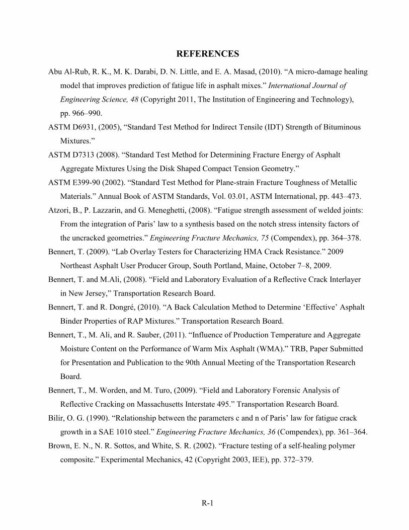
R-1

REFERENCES

Abu Al-Rub, R. K., M. K. Darabi, D. N. Little, and E. A. Masad, (2010). “A micro-damage healing

model that improves prediction of fatigue life in asphalt mixes.” International Journal of

Engineering Science, 48 (Copyright 2011, The Institution of Engineering and Technology),

pp. 966–990.

ASTM D6931, (2005), “Standard Test Method for Indirect Tensile (IDT) Strength of Bituminous

Mixtures.”

ASTM D7313 (2008). “Standard Test Method for Determining Fracture Energy of Asphalt

Aggregate Mixtures Using the Disk Shaped Compact Tension Geometry.”

ASTM E399-90 (2002). “Standard Test Method for Plane-strain Fracture Toughness of Metallic

Materials.” Annual Book of ASTM Standards, Vol. 03.01, ASTM International, pp. 443–473.

Atzori, B., P. Lazzarin, and G. Meneghetti, (2008). “Fatigue strength assessment of welded joints:

From the integration of Paris’ law to a synthesis based on the notch stress intensity factors of

the uncracked geometries.” Engineering Fracture Mechanics, 75 (Compendex), pp. 364–378.

Bennert, T. (2009). “Lab Overlay Testers for Characterizing HMA Crack Resistance.” 2009

Northeast Asphalt User Producer Group, South Portland, Maine, October 7–8, 2009.

Bennert, T. and M.Ali, (2008). “Field and Laboratory Evaluation of a Reflective Crack Interlayer

in New Jersey,” Transportation Research Board.

Bennert, T. and R. Dongré, (2010). “A Back Calculation Method to Determine ‘Effective’ Asphalt

Binder Properties of RAP Mixtures.” Transportation Research Board.

Bennert, T., M. Ali, and R. Sauber, (2011). “Influence of Production Temperature and Aggregate

Moisture Content on the Performance of Warm Mix Asphalt (WMA).” TRB, Paper Submitted

for Presentation and Publication to the 90th Annual Meeting of the Transportation Research

Board.

Bennert, T., M. Worden, and M. Turo, (2009). “Field and Laboratory Forensic Analysis of

Reflective Cracking on Massachusetts Interstate 495.” Transportation Research Board.

Bilir, O. G. (1990). “Relationship between the parameters c and n of Paris’ law for fatigue crack

growth in a SAE 1010 steel.” Engineering Fracture Mechanics, 36 (Compendex), pp. 361–364.

Brown, E. N., N. R. Sottos, and White, S. R. (2002). “Fracture testing of a self-healing polymer

composite.” Experimental Mechanics, 42 (Copyright 2003, IEE), pp. 372–379.

R-2

Buttlar, W. G., R. Roque, and N. Kim, (1996). “Accurate Asphalt Mixture Tensile Strength.”

Proceedings of the Materials Engineering Conference, Vol. 1, pp. 163–172.

Chowdary, V., and J. M. Krishnan, “Characterization of healing in sand asphalt mixtures using a

thermomechanical framework.” Proc., 2006 Airfield and Highway Pavement Specialty

Conference, April 30, 2006 – May 3, 2006, American Society of Civil Engineers, pp. 467–478.

Christensen Jr, D. W., R. Bonaquist, E. Masad, G. Rowe, S. Brown, G. Chehab, and B. Radovsky,

“Practical application of continuum damage theory to fatigue phenomena in asphalt concrete

mixtures.” Proceedings, 2005 Meeting of the Association of Asphalt Paving Technologists,

March 7, 2005 – March 9, 2005, Association of Asphalt Paving Technologists, pp. 963–1001.

Cleveland, G. S., J. W. Button, and R. L. Lytton, (2002). “Geosynthetics in flexible and rigid

pavement overlay systems to reduce reflection cracking.” Texas A&M Transportation Institute,

298 p.

Cleveland, G., R. Lytton, and J. Button, (2003). “Reinforcing Benefits of Geosynthetic Materials

in Asphalt Concrete Overlays Using Pseudo Strain Damage Theory.” 2003, Transportation

Research Board.

Cleveland, G., R. Lytton, and J. Button, (2003). “Using pseudostrain damage theory to characterize

reinforcing benefits of geosynthetic materials in asphalt concrete overlays.” Transportation

Research Record: Journal of the Transportation Research Board, No. 1849(-1), pp. 202–211.

Darabi, M. K., R. K. Abu Al-Rub, E. A. Masad, H. Chien-Wei, D. N. and Little, (2011). “A

thermo-viscoelastic-viscoplastic-viscodamage constitutive model for asphaltic materials.”

International Journal of Solids and Structures, 48 (Copyright 2010, The Institution of

Engineering and Technology), pp. 191–207.

Dave, E. V., W. G. Buttlar, G. H. Paulino, and H. H. Hilton, “Graded viscoelastic approach for

modeling asphalt concrete pavements.” Proceedings, Multiscale and Functionally Graded

Materials 2006: 15–18 Oct. 2006, AIP, pp. 736–741.

Fang, X. Q., C. Hu, and W. H. Huang, (2007). “Determination of dynamic effective properties in

functionally graded materials.” Acta Mechanica, 192 (1–4), pp. 49–63.

Germann, F. P., and R. L. Lytton, (1979). “Methodology for predicting reflection cracking life of

asphalt concrete overlays.”

R-3

Hajj, E., P. Sebaaly, J. Porras, and J. Azofeifa, (2010). “Reflective Cracking of Flexible Pavements

Phase III: Field Verification.” Research Report No. 13KJ-1, Nevada Department of

Transportation, Research Division, University of Nevada, Reno.

Harvey, J., and C. L. Monismith, (1993). “Effects of laboratory asphalt concrete specimen

preparation variables on fatigue and permanent deformation test results using Strategic

Highway Research Program a-003a proposed testing equipment,” pp. 38–48.

Huang, L., K. Cao, and M. Zeng, (2009). “Evaluation of Semicircular Bending Test for

Determining Tensile Strength and Stiffness Modulus of Asphalt Mixtures.” Journal of Testing

and Evaluation, Vol. 37, pp. 122–128.

Huang, G., Y. Wang, and S. Yu, (2005). “A new multilayered model for in-plane fracture analysis

of functionally graded materials (fgms).” Acta Mechanica Sinica, 37(1), pp. 1–8.

Huang, B., X. Shu, and Y. Tang, (2005). “Comparison of Semi-Circular Bending and Indirect

Tensile Strength Tests for HMA Mixtures.” Advances in Pavement Engineering, GSP 130.

Jacobs, M. M. J. (1995). “Crack growth in asphaltic mixes.” PhD Thesis, University of

Technology, the Netherlands.

Kallas, B. F., and V. P. Puzinauskas, (1971). “Flexure fatigue tests on asphalt paving mixtures.”

ASTM Special Technical Publication(Compendex), pp. 47–66.

Kessler, M. R. (2007). “Self-healing: A new paradigm in materials design.” Proceedings of the

Institution of Mechanical Engineers, Part G: Journal of Aerospace Engineering, 221

(Compendex), pp. 479–495.

Kim, Y. R., and D. N. Little, (1989). “Evaluation of healing in asphalt concrete by means of the

theory of nonlinear viscoelasticity.” Transportation Research Record (Compendex), pp. 198–210.

Kim, R. and H. Wen, (2002). “Fracture Energy from Indirect Tension Testing,” Journal of the

Association of Asphalt Paving Technologists, Vol. 71, pp. 779–793.

Koohi, Y., J. J. Lawrence, R. Luo, and R. L. Lytton, (2011). “Complex stiffness gradient

estimation of field-aged asphalt concrete layers using the direct tension test.” Journal of

Materials in Civil Engineering, 1 (Compendex), 401.

Kuai, H., H. J. Lee, G. Zi, and S. Mun, (2009). “Application of generalized j-integral to crack

propagation modeling of asphalt concrete under repeated loading.” Transportation Research

Record (2127), pp. 72–81.

R-4

Li, X. and M. Marasteanu, (2004). “Evaluation of the Low Temperature Fracture Resistance of

Asphalt Mixtures using the Semi-Circular Bending Test.” Journal of the Association of Asphalt

Paving Technologists, 73, pp. 401–426.

Loria-Salazar, L. (2008). “Reflective Cracking of Flexible Pavements: Literature Review, Analysis

Models, and Testing Methods.” Master’s Thesis, University of Nevada, Reno.

Majidzadeh, K., E. M. Kaufmann, and D. V. Ramsamooj, (1970). “Application of Fracture

Mechanics in the Analysis of Pavement Fatigue, Proceedings of Association of Asphalt

Pavement Technologists, 1970, Vol. 40, pp. 227–246.

Masad, E., E. Kassem, and A. Chowdhury, (2009). “Application of Imaging Technology to

Improve the Laboratory and Field Compaction of HMA.” Technical Research Report

FHWA/TX-09/0-5261-1.

Molenaar, A., A. Scarpas, X. Liu, and S. Erkens, (2002). “Semi-Circular Bending Test: Simple but

Useful?” Journal of the Association of Asphalt Paving Technologists, Vol. 71, pp. 794–815.

Mukherjee, S. and G. H. Paulino, (2003). “The elastic-viscoelastic correspondence principle for

functionally graded materials, revisited.” Transactions of the ASME. Journal of Applied

Mechanics, 70(3), pp. 359–363.

Paris, P. and E. Erdogan, (1963). “A Critical Analysis of Crack Propagation Laws.” Journal of

Basic Engineering. Transaction of the American Society of Mechanical Engineering, Series D,

1963, Vol. 85, pp. 528–883.

Pugno, N., M. Ciavarella, P. Cornetti, and A. Carpinteri, (2006). “A generalized Paris’ law for

fatigue crack growth.” Journal of the Mechanics and Physics of Solids, 54 (Copyright 2006,

The Institution of Engineering and Technology), pp. 1333–1349.

Ramsamooj, D. V. (1991). “Prediction of fatigue life of asphalt concrete beams from fracture

tests.” Journal of Testing and Evaluation, 19 (3), 231–239.

Ramsamooj, D. V. (1991). “Prediction of fatigue life of asphalt concrete beams from fracture

tests.” Journal of Testing and Evaluation, 19 (Compendex), pp. 231–239.

Schapery, R. A. (1984). “Correspondence principles and a generalized j integral for large

deformation and fracture analysis of viscoelastic media.” International Journal of Fracture,

25 (3), pp. 195–223.

Schapery, R. A. (1989). “On the mechanics of crack closing and bonding in linear viscoelastic

media.” International Journal of Fracture, 39 (1–3), pp. 163–189.

R-5

Schapery, R. A. (1975). “A theory of crack initiation and growth in viscoelastic media.”

International Journal of Fracture, 11.

Shen, S., H.-M. Chiu, and H. Huang, (2010). “Characterization of fatigue and healing in asphalt

binders.” Journal of Materials in Civil Engineering, 22 (Compendex), pp. 846–852.

SHRP. (1994). “Level One Mix Design: Material Selection, Compaction, and Conditioning”

SHRP-A-408, Strategic Highway Research Program, National Research Council, DC.

Tayebali, A. A., J. A. Deacon, and C. L. Monismith, (1996). “Development and evaluation of

dynamic flexural beam fatigue test system.” Transportation Research Record (1545), pp. 89–97.

Tex-226-F. (2004). “Indirect Tensile Strength Test.”

Tex-241-F. (2009). “Superpave Gyratory Compacting of Test Specimens of Bituminous

Materials.”

Tex-242-F. (2009). “Hamburg Wheel-tracking Test.”

Tex-248-F. (2009). “Overlay Test.”

T.O. Medani, and A. A. A. Molenaar, (2000). “A simplified practical procedures for estimation of

fatigue and crack growth characteristics of asphaltic mixes.” International Journal of Road

Materials and Pavement Design, 10.

TxDOT. (2004). “Standard Specifications for Construction and Maintenance of Highways, Streets,

and Bridges.” Austin, Texas.

TxDOT. (2009). “Texas Department of Transportation. Crack-Attenuating Mixture.” Statewide

Special Specification 3165 (04). Austin, Texas.

TxDOT. (2011). Pocket Facts: TxDOT Test Specification Manuals.

http://www.txdot.gov/business/contractors_consultants/test_procedures/tms_series.htm?series=

200-F Accessed October 2011.

Wagoner, M., W. Buttlar, and G. Paulino, (2005). “Disk-shaped Compact Tension Test for Asphalt

Concrete Fracture.” Experimental Mechanics. Vol. 45, No. 3, 2005.

Walubita, L., A. Epps Martin, S. Jung, C. Glover, E. Park, A. Chowdhury, and R. Lytton, (2004).

“Comparison of Fatigue Analysis Approaches for Two Hot Mix Asphalt Concrete (HMAC)

Mixtures.” Research Report No. FHWA/TX-05/0-4468-2, Texas A& M Transportation

Institute, Texas A&M University System, College Station, Texas.

R-6

Walubita, L. F. (2006). Comparison of fatigue analysis approaches for predicting fatigue lives of

hot-mix asphalt concrete (HMAC) mixtures, PhD Dissertation, Texas A&M University,

College Station, Texas.

Walubita, L., V. Umashankar, X. Hu, B. Jamison, F. Zhou, T. Scullion, A. Epps Martin, and S.

Dessouky, (2010). “New Generation Mix-Designs: Laboratory Testing and Construction of the

APT Test Sections.” Technical Research Report FHWA/TX-10/0-6132-1. Texas A&M

Transportation Institute.

Walubita, L. F., A. N. M. Faruk, G. Das, H. A. Tanvir, J. Zhang, and T. Scullion (2012). The

Overlay Tester: A Sensitivity Study to Improve OT Repeatability and Minimize Variability in

the OT Test Results. Technical Research Report FHWA/TX-12/0-6607-1. Texas A&M

Transportation Institute.

Wen, H., and H. Bahia, (2009). “Characterizing fatigue of asphalt binders with viscoelastic

continuum damage mechanics.” Transportation Research Record (Compendex), pp. 55–62.

Wu, X., and Y.-X. Luo, (2011). “Dynamic responses of a beam with functionally graded materials

with Timoshenko beam correction theory.” Zhendong yu Chongji/Journal of Vibration and

Shock, 30 (10), pp. 245–248.

Yoda, M. (1980). “The j-integral fracture toughness for mode ii.” International Journal of

Fracture, 16 (4), R175–R178.

Yufeng, G., and G. Wanlin, (2006). “Self-healing properties of flaws in nanoscale materials:

Effects of soft and hard molecular dynamics simulations and boundaries studied using a

continuum mechanical model.” Physical Review B (Condensed Matter and Materials Physics),

73 (Copyright 2006, The Institution of Engineering and Technology), 085411 (2006).

Zhang, J., and X. Huang, (2010). “Viscoelastoplastic-damage mechanics model of permanent

deformation in asphalt mixture.” Journal of Southeast University (Natural Science Edition), 40

(Copyright 2010, The Institution of Engineering and Technology), pp. 185–189.

Zhao, Y., and Y. R. Kim, “Time-temperature superposition for asphalt mixtures with growing

damage and permanent deformation in compression.” National Research Council, pp. 161–172.

Zhou, F. and T. Scullion, (2003). “Upgraded Overlay Tester and Its Application to Characterize

Reflection Cracking Resistance of Asphalt Mixtures.” Research Report No. FHWA/TX-04/0-

4467-1, Texas A&M Transportation Institute, Texas A&M University System, College Station,

Texas.

R-7

Zhou, F. and T. Scullion, (2005). “Overlay Tester: A Rapid Performance Related Crack Resistance

Test.” Research Report No. FHWA/TX-04/0-4467-2, Texas A&M Transportation Institute,

Texas A&M University System, College Station, Texas.

Zhou, F., T. Scullion, and R. Williammee, (2004). “Upgraded TTI Overlay Tester: A Simple

Reflective Cracking Simulation Test,” In Pavement Management, Design, and Testing.

CD-ROM. Transportation Research Board of the National Academies, Washington, D.C.

Zhu, G., S. Wu, R. Liu, and L. Zhou, (2009). “Study on the fatigue property for aged asphalt

mixtures by using four point bending tests.” 6th International Forum on Advanced Material

Science and Technology, IFAMST 2008, June 12, 2008 – June 14, 2008, Trans Tech

Publications Ltd, Hong Kong, China, pp. 289–294.

A-1

APPENDIX A: OT MACHINE CHECK, CALIBRATION, AND VERIFICATION PRIOR TO ROUND-ROBIN TESTING

Figure A-1. Example OT Displacement Error Deviation prior to Calibration.

Figure A-2. Comparison of OT Machine Peak Loads (Type D Mix).

OT machines Error from 0.025″ Comment_____________________________________________________________________

1) TxDOT Old 6007 +0.0011″ Higher displacement less cycles2) TxDOT New 7001 -0.0001″ Same as 1002

3) TTI Old 7002 -0.0002″ Lower displacement more cycles4) TTI New 1002 -0.0001″ Same as 7001

TxDOT Old TxDOT New TTI Old TTI New

Sample# 1 531 639 549 203

Sample# 2 540 502 461 478

Sample# 3 488 448 499 470

Sample# 4 576 382 546 408

Sample# 5 504 591 518 489

Avg (best 3) 525 577 538 479

CV % (best 3) 4 12 3 2

Avg (all) 528 512 515 410

CV % (all) 6 20 7 29

Avg overall 491

Stdev overall 55

COV overall 11.1%

A-2

Figure A-3. Comparison of Loads Reduction at Test Termination (Type D Mix).

Table A-1. Comparison of AV and OT Cycle Results (Type D Mix).

Item TxDOT Old TxDOT New TTI Old TTI New

AV

(avg, all 5 replicates)

7 7 7 7

COV

(all 5 replicates)

2% 2% 2% 6%

OT cycles

(avg, all 5 replicates)

273 260 319 209

COV

(all 5 replicates)

49% 50% 59% 19%

TxDOT Old(%Pmax)

TxDOT New(%Pmax)

TTI Old(%Pmax)

TTI New(%Pmax)

Sample# 1 37 (7%) 45 (7%) 17 (3%) 15 (7%)

Sample# 2 38 (7%) 35 (7%) 32 (7%) 34 (7%)

Sample# 3 34 (7%) 31 (7%) 47 (9%) 33 (7%)

Sample# 4 40 (7%) 27 (7%) 59 (11%) 33 (7%)

Sample# 5 35 (7%) 41 (7%) 37 (7%) 29 (7%)

Avg (best 3) 38 (7%) 40 (7%) 39 33 (7%)

CV % (best 3) 4 13 20 2

Avg (all) 37 (7%) 36 (7%) 38 (7%) 29 (7%)

CV % (all) 7 20 42 27

Avg overall 35

Stdev overall 10

COV overall 27.5%

A-3

Figure A-4. Method Adapted for Measuring Crack Widths in the Field (by Bryan Wilson).

Figure A-5. Average Crack Widths (Inches) Measured at Different Field Sections (by Bryan Wilson).

A-4

Figure A-6. Transverse Cracked Pavement Sections at Riverside Campus and Pecos RTC (by Bryan Wilson).

Figure A-7. Crack Movement (Inches) of Various Pavements at Riverside Campus (by Bryan Wilson).

0.00

0.01

0.02

0.03

0.04

0.05

A B C D E F G H

Cha

nge

in C

rack

Wid

th (i

n.)

Pavement Structure

OT setting, 0.025

Cement-Treated LTB+CTB Untreated Lime-Treated Concrete

Avg. pave. tempWarm: 108°F

Cool: 44°F

A-5

Figure A-7. Crack Movement Measurements (Inches) at Pecos RTC (by Bryan Wilson).

Figure A-7. Transverse Spacing (ft) versus Crack Movement (Inches) at Riverside Campus (by Bryan Wilson).

0.000.010.020.030.040.050.060.070.080.09

1 2 3 4 5 6 7 8 9 10 1 2 3 4 5 6 7 8 9

Cha

nge

in C

rack

Wid

th (i

n.)

Measured CrackNewer Pavement Older Pavement

0.060 in. 0.063 in.

OT setting, 0.025

Avg. pave. tempWarm: 88°F

Cool: 33°F

B-1

APPENDIX B: OT PARALLEL TESTING WITH TXDOT-CST (AUSTIN)

Table B-1. Work Plans for Parallel OT Testing with TxDOT-CST. (All aggregate batching done at TTI)

Table B-2. Example of Parallel OT Testing Results for a Type D Mix.

Phase Samples TTI Tasks TxDOT Tasks

Ia 5 -Mixing, molding -Cutting, drying, AV, gluing -Testing

---

Ib 5 --- -Mixing, molding -Cutting, drying, AV, gluing -Testing

IIa 5 -Testing -Mixing, Molding -Cutting, drying, AV, gluing

IIb 5 -Mixing, molding -Cutting, drying, AV, gluing

-Testing

IIIa 5 -Cutting, drying, AV, gluing -Testing

-Mixing, molding

IIIb 5 -Mixing, molding

-Cutting, drying, AV, gluing -Testing

Atlanta Type D: 5.1%PG 64-22 + Quartzite + 20% RAPUS 59 SB (Atlanta District; Panola County)

OT Cycles

TxDOT-CST TTI

Sample# 1 294 309

Sample# 2 241 121

Sample# 3 197 334

Sample# 4 257 269

Sample# 5 306 240

Avg (all) 286 255

COV (all) 9.0% 32.6%

Avg (best 3) 259 304

COV (best 3) 17% 11%

C-1

APPENDIX C: LOAD-DISPLACEMENT RESPONSE CURVES FOR MONOTONIC LOADING CRACK TESTS

Figure C-1. OTM Testing – IH 35 Type B Mix.

Figure C-2. OTM Testing – SH 121 CAM Mix.

0

100

200

300

400

500

600

0 0.05 0.1 0.15

Load

(lb)

Displacement (in)

AverageOT(M)-1OT(M)-2OT(M)-3

Fracture Energy Tensile Str.

Sample# (J/m2) (lb-in/in2) (psi) (Mpa) Strain (mm/mm) FE Index

OTM1 855 4.882 100 0.689 0.1513 4.94

OTM2 592 3.379 90 0.623 0.1789 4.47

OTM3 472 2.697 107 0.742 0.0969 1.62

Average 640 3.653 99 0.685 0.1423 3.68

COV 30.6% 30.6% 8.7% 8.7% 29.3% 48.8%

Fracture Energy Tensile Str.

Sample# (J/m2) (lb-in/in2) (psi) (Mpa) Strain (mm/mm) FE Index

OTM1 848 4.841 62 0.430 0.1989 10.31

OTM2 849 4.849 59 0.411 0.3807 20.70

OTM3 663 3.784 54 0.372 0.3189 14.96

Average 786 4.491 58 0.404 0.2995 15.32

COV 13.6% 13.6% 7.4% 7.4% 30.9% 34.0%

0

50

100

150

200

250

300

0 0.02 0.04 0.06 0.08 0.1 0.12 0.14

Load

(lb)

Displacement (in)

Average

OT(M)-1

OT(M)-2

OT(M)-3

C-2

Figure C-3. OTM Testing – US 59 Type D Mix.

Figure C-4. OTM Testing – Chico Type D (4.5% AC) Mix.

Fracture Energy Tensile Str.

Sample# (J/m2) (lb-in/in2) (psi) (Mpa) Strain (mm/mm) FE Index

OTM1 1275 7.28 183 1.26 0.131 5.85

OTM2 1438 8.21 210 1.45 0.125 4.38

OTM3 1711 9.78 185 1.28 0.198 6.10

Average 1475 8.42 193 1.33 0.151 5.44

COV 14.9% 14.9% 7.9% 7.9% 27.0% 17.0%

0

100

200

300

400

500

600

700

800

0 0.02 0.04 0.06 0.08 0.1 0.12 0.14

Load

(lb)

Displacement (in)

Average

OT(M)-1

OT(M)-2

OT(M)-3

0

100

200

300

400

500

600

0 0.02 0.04 0.06 0.08 0.1 0.12 0.14

Load

(lb-

f)

Displacement (in)

OT(M)-1OT(M)-2OT(M)-3Average

Fracture Energy Tensile Str.

Sample# (J/m2) (lb-in/in2) (psi) (Mpa) Strain (mm/mm) FE Index

OTM1 742 4.235 105 0.721 0.1213 3.2739

OTM2 740 4.228 100 0.69 0.1225 3.4506

OTM3 703 4.014 117 0.807 0.1525 3.4893

Average 728 4.159 107 0.739 0.1321 3.4046

COV 3.0% 3.0% 8.2% 8.2% 13.4% 3.4%

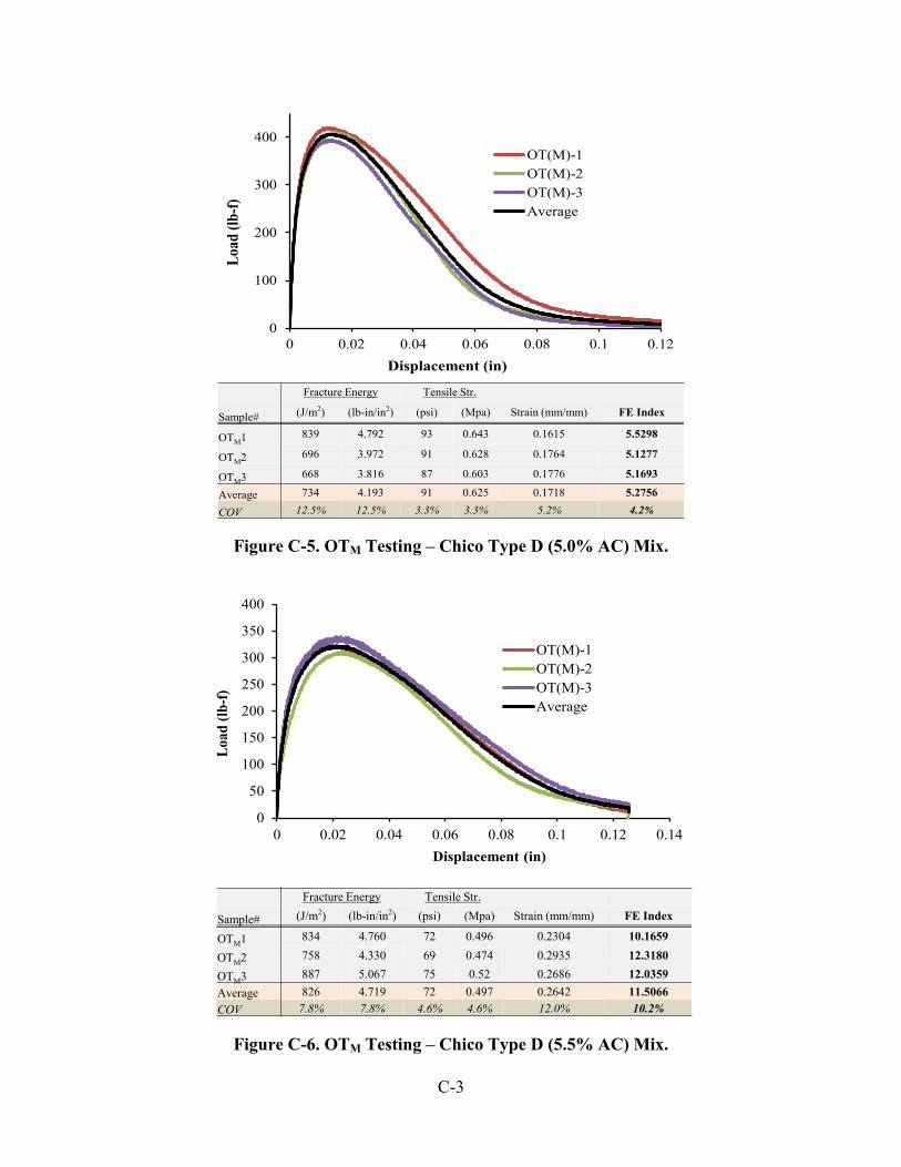
C-3

Figure C-5. OTM Testing – Chico Type D (5.0% AC) Mix.

Figure C-6. OTM Testing – Chico Type D (5.5% AC) Mix.

0

100

200

300

400

0 0.02 0.04 0.06 0.08 0.1 0.12

Load

(lb-

f)

Displacement (in)

OT(M)-1OT(M)-2OT(M)-3Average

Fracture Energy Tensile Str.

Sample# (J/m2) (lb-in/in2) (psi) (Mpa) Strain (mm/mm) FE Index

OTM1 839 4.792 93 0.643 0.1615 5.5298

OTM2 696 3.972 91 0.628 0.1764 5.1277

OTM3 668 3.816 87 0.603 0.1776 5.1693

Average 734 4.193 91 0.625 0.1718 5.2756

COV 12.5% 12.5% 3.3% 3.3% 5.2% 4.2%

Fracture Energy Tensile Str.

Sample# (J/m2) (lb-in/in2) (psi) (Mpa) Strain (mm/mm) FE Index

OTM1 834 4.760 72 0.496 0.2304 10.1659

OTM2 758 4.330 69 0.474 0.2935 12.3180

OTM3 887 5.067 75 0.52 0.2686 12.0359Average 826 4.719 72 0.497 0.2642 11.5066COV 7.8% 7.8% 4.6% 4.6% 12.0% 10.2%

0

50

100

150

200

250

300

350

400

0 0.02 0.04 0.06 0.08 0.1 0.12 0.14

Load

(lb-

f)

Displacement (in)

OT(M)-1OT(M)-2OT(M)-3Average

C-4

Figure C-7. OTM Testing – Chico Type D Mix – AC Variation Summary.

Figure C-8. IDT Testing – IH 35 Type B Mix.

ACFracture Energy Tensile Str.

(J/m2) (lb-in/in2) (psi) (Mpa) Strain (mm/mm) FE Index

4.5% 728 4.159 107 0.739 0.1321 3.405.0% 734 4.193 91 0.625 0.1718 5.285.5% 826 4.719 72 0.497 0.2642 11.51

050

100150200250300350400450500

0 0.02 0.04 0.06 0.08 0.1 0.12 0.14

Load

(lb-

f)

Displacement (in)

4.5% AC

5.0% AC

5.5% AC

0

500

1000

1500

2000

2500

3000

0 0.02 0.04 0.06 0.08 0.1 0.12 0.14

Load

(lb-

f)

Displacement (in)

IDT-1

IDT-2

IDT-3

Average

Sample# (J/m2) (lb-in/in2) (psi) (Mpa) Strain (mm/mm) FE IndexIDT1 135 0.771 103 0.712 0.0135 1.6762IDT2 134 0.766 99 0.682 0.0164 2.1158IDT3 140 0.799 107 0.736 0.0148 1.8443Average 136 0.779 103 0.710 0.0149 1.8788COV 2.3% 2.3% 3.8% 3.8% 9.9% 11.8%

Tensile Str.Fracture Energy

C-5

Figure C-9. IDT Testing – SH 121 CAM Mix.

Figure C-10. IDT Testing – US 59 Type D Mix.

0

500

1000

1500

2000

2500

0 0.05 0.1 0.15 0.2 0.25

Load

(lb-

f)

Displacement (in)

IDT-1IDT-2IDT-3Average

Sample# (J/m2) (lb-in/in2) (psi) (Mpa) Strain (mm/mm) FE IndexIDT1 216 1.235 81 0.559 0.0341 8.6595IDT2 239 1.365 78 0.538 0.0353 10.2769IDT3 222 1.269 79 0.544 0.0325 8.7048Average 226 1.290 79 0.547 0.0340 9.2138COV 5.2% 5.2% 2.0% 2.0% 4.1% 10.0%

Fracture Energy Tensile Str.

0

500

1000

1500

2000

2500

3000

3500

0 0.02 0.04 0.06 0.08 0.1 0.12 0.14

Load

(lb-

f)

Displacement (in)

IDT-1IDT-2IDT-3Average

Sample# (J/m2) (lb-in/in2) (psi) (Mpa) Strain (mm/mm) FE IndexIDT1 210 1.199 131 0.905 0.0231 3.5214IDT2 189 1.077 128 0.881 0.0177 2.4818IDT3 180 1.027 122 0.841 0.0161 2.2634Average 193 1.101 127 0.876 0.0190 2.7555COV 8.1% 8.1% 3.7% 3.7% 19.4% 24.4%

Fracture Energy Tensile Str.

C-6

Figure C-11. IDT Testing – Chico Type D (4.5% AC) Mix.

Figure C-12. IDT Testing – Chico Type D (5.0% AC) Mix.

0

500

1000

1500

2000

2500

0 0.02 0.04 0.06 0.08 0.1 0.12 0.14

Load

(lb-

f)

Displacement (in)

IDT-1IDT-2IDT-3Average

Sample# (J/m2) (lb-in/in2) (psi) (Mpa) Strain (mm/mm) FE IndexIDT1 113 0.647 87 0.601 0.0147 1.8214IDT2 111 0.637 82 0.567 0.0145 1.8669IDT3 116 0.664 86 0.593 0.0143 1.8455Average 114 0.649 85 0.587 0.0145 1.8446COV 2.2% 2.2% 3.1% 3.1% 1.4% 1.2%

Fracture Energy Tensile Str.

0200400600800

100012001400160018002000

0 0.02 0.04 0.06 0.08 0.1 0.12 0.14

Load

(lb-

f)

Displacement (in)

IDT-1IDT-2IDT-3Average

Sample# (J/m2) (lb-in/in2) (psi) (Mpa) Strain (mm/mm) FE IndexIDT1 120 0.686 75 0.514 0.0193 2.9564IDT2 131 0.746 80 0.551 0.0177 2.7610IDT3 121 0.692 71 0.487 0.0166 2.7104Average 124 0.708 75 0.517 0.0179 2.8093COV 4.7% 4.7% 6.2% 6.2% 7.5% 4.6%

Fracture Energy Tensile Str.

C-7

Figure C-12. IDT Testing – Chico Type D (5.5% AC) Mix.

Figure C-13. IDT Testing – Chico Type D Mix – AC Variation Summary.

0

500

1000

1500

2000

2500

3000

0 0.02 0.04 0.06 0.08 0.1 0.12 0.14 0.16

Load

(lb-

f)

Displacement (in)

IDT-1IDT-2IDT-3Average

Sample# (J/m2) (lb-in/in2) (psi) (Mpa) Strain (mm/mm) FE IndexIDT1 199 1.138 112 0.774 0.0189 3.1873IDT2 209 1.193 112 0.773 0.0205 3.6402IDT3 201 1.147 105 0.722 0.0217 3.9548Average 203 1.159 110 0.756 0.0204 3.5941COV 2.6% 2.6% 3.9% 3.9% 6.9% 10.7%

Fracture Energy Tensile Str.

0

500

1000

1500

2000

2500

3000

0 0.02 0.04 0.06 0.08 0.1 0.12 0.14

Load

(lb-

f)

Displacement (in)

4.5% AC

5.0% AC

5.5% AC

ACFracture Energy Tensile Str.(J/m2) (lb-in/in2) (psi) (Mpa) Strain (mm/mm) FE Index

4.5% 114 0.649 85 0.587 0.0145 1.845.0% 124 0.708 75 0.517 0.0179 2.815.5% 203 1.159 110 0.756 0.0204 3.59

C-8

Figure C-14. SCB Testing – IH 35 Type B Mix.

Figure C-15. SCB Testing – SH 121 CAM Mix.

050

100150200250300350400450

0 0.01 0.02 0.03 0.04 0.05

Load

(lb-

f)

Displacement (in)

SCB-1

SCB-2

SCB-3

Average

Fracture Energy Tensile Str.

Sample#(J/m2) (lb-in/in2) (psi) (Mpa) Strain

(mm/mm) FE Index

SCB1 102 0.585 167 1.152 0.0053 0.67SCB2 177 1.008 243 1.672232 0.0064 0.97SCB3 156 0.891 200 1.375638 0.0069 1.12Average 145 0.828 203 1.400 0.0062 0.92COV 26.4% 26.4% 18.6% 18.6% 13.3% 24.7%

0

50

100

150

200

250

300

0 0.02 0.04 0.06 0.08 0.1

Load

(lb-

f)

Displacement (in)

SCB-1SCB-2SCB-3Average

Sample# (J/m2) (lb-in/in2) (psi) (Mpa) Strain (mm/mm) FE IndexSCB1 258 1.475 154 1.059 0.0124 4.3298SCB2 301 1.721 146 1.008 0.0235 10.0710SCB3 281 1.607 141 0.971 0.0205 8.4945Average 280 1.601 147 1.013 0.0188 7.6318COV 7.7% 7.7% 4.4% 4.4% 30.6% 38.9%

Fracture Energy Tensile Str.

C-9

Figure C-16. SCB Testing – US 59 Type D Mix.

Figure C-17. SCB Testing – Chico Type D (4.5% AC) Mix.

0

100

200

300

400

500

600

0 0.01 0.02 0.03 0.04 0.05 0.06 0.07

Loa

d (lb

-f)

Displacement (in)

SCB-1SCB-2SCB-3Average

Sample# (J/m2) (lb-in/in2) (psi) (Mpa) Strain (mm/mm) FE IndexSCB1 347 1.983 333 2.298 0.0105 2.28SCB2 186 1.063 207 1.429 0.0083 1.55SCB3 322 1.836 254 1.751 0.0135 3.54Average 285 1.627 265 1.826 0.0108 2.46COV 30.4% 30.4% 24.1% 24.1% 23.9% 40.9%

Fracture Energy Tensile Str.

Sample# (J/m2) (lb-in/in2) (psi) (Mpa) Strain (mm/mm) FE IndexSCB1 152 0.869 203 1.401 0.0099 1.5340SCB2 201 1.151 180 1.24 0.0089 2.0626SCB3 170 0.973 193 1.329 0.0071 1.2964Average 175 0.997 192 1.324 0.0086 1.6310COV 14.3% 14.3% 6.1% 6.1% 16.5% 24.0%

Fracture Energy Tensile Str.

0

50

100

150

200

250

300

350

0 0.01 0.02 0.03 0.04 0.05 0.06

Loa

d (lb

-f)

Displacement (in)

SCB-1SCB-2SCB-3Average

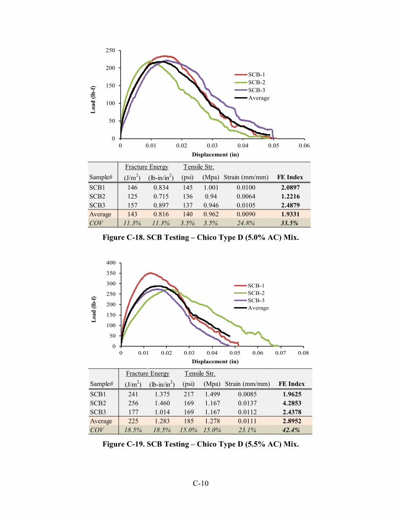
C-10

Figure C-18. SCB Testing – Chico Type D (5.0% AC) Mix.

Figure C-19. SCB Testing – Chico Type D (5.5% AC) Mix.

0

50

100

150

200

250

0 0.01 0.02 0.03 0.04 0.05 0.06

Load

(lb-

f)

Displacement (in)

SCB-1SCB-2SCB-3Average

Sample# (J/m2) (lb-in/in2) (psi) (Mpa) Strain (mm/mm) FE IndexSCB1 146 0.834 145 1.001 0.0100 2.0897SCB2 125 0.715 136 0.94 0.0064 1.2216SCB3 157 0.897 137 0.946 0.0105 2.4879Average 143 0.816 140 0.962 0.0090 1.9331COV 11.3% 11.3% 3.5% 3.5% 24.8% 33.5%

Fracture Energy Tensile Str.

0

50

100

150

200

250

300

350

400

0 0.01 0.02 0.03 0.04 0.05 0.06 0.07 0.08

Load

(lb-

f)

Displacement (in)

SCB-1SCB-2SCB-3Average

Sample# (J/m2) (lb-in/in2) (psi) (Mpa) Strain (mm/mm) FE IndexSCB1 241 1.375 217 1.499 0.0085 1.9625SCB2 256 1.460 169 1.167 0.0137 4.2853SCB3 177 1.014 169 1.167 0.0112 2.4378Average 225 1.283 185 1.278 0.0111 2.8952COV 18.5% 18.5% 15.0% 15.0% 23.1% 42.4%

Fracture Energy Tensile Str.

C-11

Figure C-20. SCB Testing – Chico Type D Mix – AC Variation Summary.

0

50

100

150

200

250

300

350

0 0.01 0.02 0.03 0.04 0.05 0.06

Load

(lb-

f)

Displacement (in)

4.5% AC

5.0% AC

5.5% AC

AC (J/m2) (lb-in/in2) (psi) (Mpa) Strain (mm/mm) FE Index4.5% 175 0.997 192 1.324 0.0086 1.635.0% 143 0.816 140 0.962 0.0090 1.935.5% 225 1.283 185 1.278 0.0111 2.90

Fracture Energy Tensile Str.

D-1

APPENDIX D: ADVANCED OT DATA ANALYSIS METHODS USING ENERGY CONCEPT AND NUMERICAL MODELING

The methodology that will be described in this chapter is a novel approach to analyze the

OT test results based on the linear viscoelasticity and fracture mechanics principles. The

methodology uses a Finite Element code integrated with a user-defined material to find the strain

profiles above the tip of the crack for both laboratory and aged specimen.

HMA layers under different repeated loading and rest periods experience both fatigue and

healing processes. The tests are costly and time-consuming, and the results are highly variable.

Current methods of evaluating these phenomena using the OT rely on counting the number of

load repetitions until the crack breaks through the sample.

This research provides a novel analysis method based on the viscoelastic fracture

mechanics and Finite Element modeling to predict the actual crack growth rate in asphalt mixes

both in the laboratory compacted and field samples using the Overlay Tester. Furthermore, the

new method uses viscoelastic fracture mechanics principles to find the fracture and healing

properties of the asphalt mixes. The resulting test is fast, less costly and more repeatable then the

previous methods using the Overlay Tester.

Testing lab compacted specimens have determined and improved the precision of the test

method. The COV of the laboratory compacted mixture undamaged properties are comparable

with the test results.

THE BACKGROUND OF THE OT DATA ANALYSIS METHODS Asphalt layers experience the repeated loading, unloading as well as the rest periods

because of the traffic and environmental conditions. The crack propagation from the bottom to

the top and vice versa is a prominent distress in the asphalt layers. Fortunately, each one of these

phenomena can be well explained by mechanistic-based models and various research projects

have been conducted to develop and use such models.

Different approaches have been used to characterize the crack initiation and propagation in

asphalt layers, namely, conventional fatigue crack analysis (Harvey and Monismith, 1993,

Ramsamooj, 1991, Tayebali et al., 1996), continuum damage mechanics, and fracture mechanics.

D-2

The traditional tests to measure the fatigue cracking susceptibility of mixes such as the

four-point bending beam test, are very expensive and time-consuming (Kallas and Puzinauskas,

1971, Ramsamooj, 1991, Zhu et al., 2009)

The continuum damage mechanics approach basically states that the micro structure of

materials changes with deformations caused by external loadings without focusing on the crack

initiation and propagation. Subsequently, the micro damage process results in the loss in material

properties such as stiffness. Various models have been developed to explain these phenomena in

different materials including some recent studies in HMA (Abu Al-Rub et al., 2010, Christensen

Jr. et al., 2005, Darabi et al., 2011, Wen and Bahia, 2009, Zhang and Huang, 2010, Zhao and

Kim, 2003).

This study is based on viscoelastic fracture mechanics. The fracture mechanics approach

focuses directly on the crack geometry, initiation, and propagation mechanisms. This approach is

based on Paris’s law for crack propagation theory. However, the stress intensity factor in Paris’s

law applies only to elastic materials (Paris and Erdogan, 1963).

In viscoelastic media, the generalized J-integral based on the correspondence principle

and pseudo strain energy concepts proposed by Schapery, is a powerful principle to address the

crack propagation process (Cleveland et al., 2003, Kuai et al., 2009, Schapery, 1984, Schapery,

1975).

Asphalt like other viscoelastic materials restores part of its strength by healing. The study

of the fracture or damage properties without considering the healing is incomplete and results in

an underestimation of the number of load cycles to reach failure. Various research studies

focused on the self-healing in different materials namely polymers and asphalt in recent years

(Abu Al-Rub et al., 2010, Brown et al., 2002, Chowdary and Krishnan, 2006, Kessler, 2007, Kim

and Little, 1989, Schapery, 1989, Shen et al., 2010, Yufeng and Wanlin, 2006).

The Texas OT is a capable multipurpose test apparatus. The OT was originally developed

to determine the reflection cracking resistance of hot mix asphalt mixtures used in overlays over

concrete joints (Germann and Lytton, 1979). This machine also has been used to study the

behavior of the geosynthetic fabrics and grids inside the asphalt layers based on fracture

mechanics concepts (Cleveland et al., 2003, Cleveland et al., 2002).

As shown in Figure D-1, the OT machine consists of two steel plates. One plate is fixed

and the other can move back and forth to apply the desired repeating displacement. This machine

D-3

has been modified several times since its first prototype (Germann and Lytton, 1979) and the

latest version is more precise and portable. In this later model, specimens with the standard size

of 150 mm long, 75 mm wide and 38 mm high can be tested. These specimens with this size can

be easily cut from the cylindrical mixes that the Gyratory compactor has compacted in the

laboratory or cores taken from the field. Still in the same Figure D-1, the specimen is glued on

the aluminum plates and subsequently the plates are mounted and fixed on the machine’s steel

platforms using pins (Zhou and Scullion, 2005). The data acquisition system records the time,

load, opening displacement, and temperature during the OT test. Figure D-2 shows the OT

machine during the test.

Figure D- 1. The OT Test Setup.

Figure D-2. The OT Machine during Testing.

D-4

The simplicity of the test led to its use as an index test for fatigue because in both

reflection cracking and fatigue, the active mechanism is crack growth. The OT was selected to be

used together with the Hamburg Wheel Tracking Test (HWTT) to establish a balanced asphalt

mix design procedure to account for both fatigue and rutting distresses (Zhou et al., 2007). This

test was expected to be a good surrogate for the expensive and time-consuming beam fatigue

tests (Kallas and Puzinauskas, 1971, Ramsamooj, 1991, Zhu et al., 2009).

The current OT analysis method relies on counting the load cycles to the failure and the

failure criterion is satisfied when the initial maximum load is reduced by 93 percent. The

resulting count on companion samples has proven to give a large variability. Especially, this

method does not work well with coarse graded mixes and the COV is over 30 percent (Walubita

et al., 2009).

The test method modifications and sample preparation techniques that TTI researchers

conducted have reduced the variability of the results. This variability has several causes, all of

which will be explained at the conclusion of this study. The study reported in this research was

undertaken to determine the cause of the high degree of variability and to develop methods of

using OT data that are more consistent and precise. This has been accomplished through the

application of fracture mechanics.

This study uses a novel method to analyze the OT output to achieve accurate crack

growth prediction using the principles of viscoelastic fracture mechanics and finite element (FE)

simulation (Schapery, 1975). The FE simulation of the test has been developed and it was a key

to understanding the energy release pattern as the crack grows.

Research has been conducted recently at TTI in order to find Paris’s law constants. In this

research, the crack length in each load cycle is measured with a Digital Correlation System

(DIC). The results of this work indicated that the crack grows rapidly during the first few load

cycles and after that the rate of growth decreases substantially with time (Jacobs, 1995,

T. O. Medani and Molenaar, 2000, Zhou et al., 2007, Zhou and Scullion, 2006).

In this research, the pseudo strain energy concept and Paris’s law were tailored according

to the OT test conditions to obtain fracture and healing properties of the asphalt mixes in the

same test. By applying this methodology, the OT can be used not only to obtain the number of

load cycles to reach a standard crack length, but also the fracture and healing properties of the

asphalt mixes for different quality assurance and performance prediction purposes.

D-5

This procedure has been extended for use with the field-aged specimens with a stiffness

gradient rather than uniform modulus with depth. The field layers can be tested for both top-down

and bottom-up fatigue cracking by placing the specimen in upright or inverted positions. However,

testing aged asphalt layers requires specific analytical and test procedures due to the stiffness

gradient and the high brittleness of the specimens. For instance, the opening size should be

reduced in field-aged specimens because the field-aged layers are very brittle.

This study will describe a testing protocol that includes the extraction of the field cores,

Direct Tension (DT) test, and OT test to calculate the viscoelastic properties of the field-aged

asphalt concrete mixtures. The aged asphalt concrete layer can be categorized as a Functionally

Graded Material (FGM) due to its stiffness gradient profile. The response of these materials to

different loading and temperature scenarios have been studied in various research projects (Fang et

al., 2007, Huang et al., 2005, Mukherjee and Paulino, 2003, Wu and Luo, 2011). A user-defined

material subroutine (UMAT) in the finite element software ABAQUS was developed to simulate

the response of the aged asphalt layers as functionally graded materials under repeated loadings.

The FE program output is used in a constitutive model to predict the crack growth in a field asphalt

layer under repeated loading. The FE model together with constitutive fracture mechanics-based

model is able to estimate the crack growth rate, fracture properties, and healing properties of the

field-aged asphalt mixtures.

METHODOLOGY The methodology will be described in this research will include three main modules:

• Finite Element Model to find the strain profiles above the crack tip.

• The crack growth analysis module.

• The fracture and healing characterization module.

Figure D-3 illustrates the three main modules of the methodology. There is also some

modification in the test procedure. 1E and 1m are the undamaged tensile mixture properties that

regression analysis determines.

D-6

Figure D- 3. The Analysis of the Laboratory Compacted Specimen via OT Test.

Finite Element Duplication of the Test Boundary Conditions

As part of this task, the test procedure was simulated using ABAQUS. The test is

modeled in a 2D format for an elastic material. It was assumed that Poisson’s ratio is 0.3 for

modeling purposes.

Figure D-4 shows the boundary conditions used in the FE model. As shown in Figure D-3,

the left portion of the specimen is fixed and the right portion moves back and forth in the

horizontal direction. The crack initiates from the bottom of the specimen above the opening and

closing joint, and grows vertically to the top.

Figure D-4. The Boundary Conditions of the FE Model.

The crack with different lengths was modeled and the contour integral method was used

to define the crack tip function. Figure D-5 shows the deformed specimen and the corresponding

principal stress distribution in the specimen when the crack length is 15.875 mm and the opening

is 0.635 mm.

OT-Step 1(UndamagedProperties)

OT-Step 2(DamagedProperties)

Crack Growth Module

Finite ElementModel

CutFracture and

Healing Module

150 mm

38 m

m

D-7

Since the test is displacement controlled, the strain profiles above the tip of the crack

remain the same, regardless of the magnitude of the elastic modulus. This information was used

to predict the crack length in each cycle, as the strain profiles above the tip of the crack depend

only on the maximum displacement magnitude.

Figure D-5. The Deformed Specimen and the Corresponding Principal Stress Distribution.

The computed strain profiles for four different crack lengths are plotted against specimen

depth in Figure D-6. As seen in Figure D-6, as the crack advances, the area under the strain

profiles in the intact material decreases. In this study, the change of the area under the strain

curve at different crack lengths was used to estimate the actual crack length in each load cycle. In

specimens thicker than 40 mm, the strain in the upper 10 mm becomes compressive.

D-8

Figure D-6. The Strain Profiles above the Tip Of the Crack at Different Crack Lengths.

(C = Crack Length)

The Effect of the Displacement (Opening) and the Thickness on the Test Results

The counting the number of the load cycles to failure has been used to compare the

asphalt mixtures; however, users have reported substantial variability in this method. This may

happen for different reasons. A sensitivity analysis was conducted to compare the strain profile

contours above the crack. The results showed that in the specimens thicker than 38 mm

(1.5 inches) the upper parts will be in the compression or very small tensile strains; therefore, as

a crack enters these low tensile strain or compressive zones, the crack growth rate decreases

significantly.

Figure D-7 shows the strain profiles above two specimens with the same crack length and

different thicknesses. As shown in Figure D-7, the thicker specimen has a compressive zone at

the top of the sample. This zone delays the crack growth. Unlike the method of counting cycles

to failure, the methodology that is described in this research estimates the crack growth function

D-9

as it varies with the load cycles that, in turn, is already related to the strain profiles above the

crack tip. Therefore, the problem of the high cycle count variability only occurs in the case in

which the load cycles are counted to failure.

Figure D-7. The Effect of the Specimen Thickness on the Strain Contours above the Crack.

(d = sample thickness)

Additionally, the effect of the destructive displacement opening is not very significant in

changing the size of the compressive zone above the crack. As expected, the larger displacement

results in a larger compressive and tensile strains; unlike the thickness, however, the shape of the

strain contours above the crack remains the same. Figure D-8 shows the strain profiles above the

crack for different maximum openings.

d=1.5 inches

d=2 inches

D-10

Figure D-8. The Effect of the Gap Opening on the Strain Contours above the Crack Tip.

(s = Gap Opening)

s=0.00625 inches

s=0.0125 inches

s=0.01875 inches

s=0.025 inches

s=0.03125 inches

s=0.0375 inches

D-11

The Stress Intensity Factor and the J-integral

The FE simulation results show that the energy release rate decreases as the crack grows.

In order to understand the crack propagation process in the OT test, the stress intensity factor and

J-integral were calculated with time as the crack grows. The FE simulation was used to obtain

the changes in the stress intensity factor and J-integral against crack length. The crack in the OT

test is a Mode І tensile crack. The size of the stress intensity factor, KΙ controls the crack growth

rate, which is defined in Equation D-1 as:

K Cσ πΙ = (D-1)

where σ is stress and C is the half crack length.

Figure D-9 shows that the stress intensity factor for Mode І reduces significantly as the

crack grows.

Figure D-9. The Stress Intensity Factor Versus Crack Length.

The same trend can be seen in Figure D-10 for the J-integral (strain energy release rate),

which is related to fracture toughness under Mode І loading at the tip of the crack (Yoda, 1980). 2

2 1( )J KEν

Ι Ι

−= (D-2)

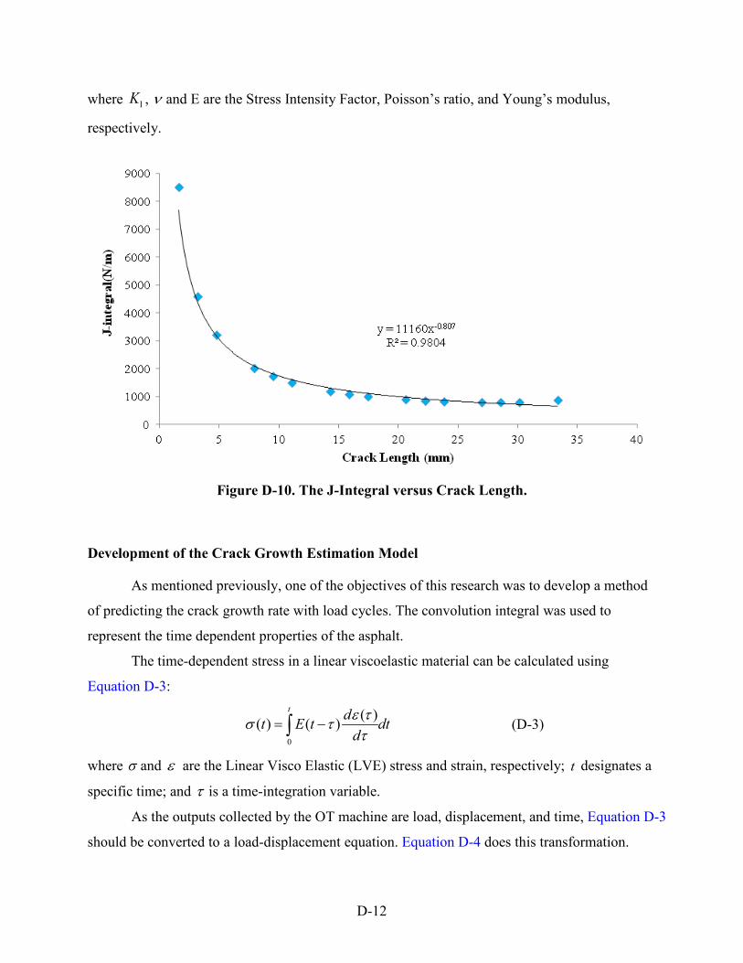
D-12

where KΙ , ν and E are the Stress Intensity Factor, Poisson’s ratio, and Young’s modulus,

respectively.

Figure D-10. The J-Integral versus Crack Length.

Development of the Crack Growth Estimation Model

As mentioned previously, one of the objectives of this research was to develop a method

of predicting the crack growth rate with load cycles. The convolution integral was used to

represent the time dependent properties of the asphalt.

The time-dependent stress in a linear viscoelastic material can be calculated using

Equation D-3:

0

( )( ) ( )t dt E t dt

dε τσ ττ

= −∫ (D-3)

where σ and ε are the Linear Visco Elastic (LVE) stress and strain, respectively; t designates a

specific time; and τ is a time-integration variable.

As the outputs collected by the OT machine are load, displacement, and time, Equation D-3

should be converted to a load-displacement equation. Equation D-4 does this transformation.

D-13

( )( ) LVEP ttA

σ = (D-4)

where ( )LVEP t is the measured viscoelastic force and A is the intact area (the area above the

crack tip).

The first part of the test is designed to obtain the undamaged properties of the asphalt

mixes. The displacements in the nondestructive test are limited to ensure that there is no crack

growth.

The relaxation modulus is given by the form shown in Equation D-5. 1

1( ) .( )mE t E tτ τ− = − (D-5)

where 1E and 1m are the undamaged tensile mixture properties, which are determined by

regression analysis. The loading pattern for this test is shown in Figure D-11.

Figure D-11. The Loading Pattern in the OT Test.

The data from the first load cycle in the nondestructive test was used to obtain the

undamaged properties. First the percentage of the maximum opening at the time 1t t< is

calculated using Equation D-6:

0 1

( )u t tu t

= (D-6)

where ( )u t is the displacement at time t and 0u is the maximum displacement.

The elastic strain at time 1t t< and opening u for the no-crack condition are shown in

Equation D-7. 2

0 21

( 0, ( ), ) ( 0, , ) tc u t z c u zt

ε ε= = = (D-7)

r -r

u0

0 t

u

t1 t2 t3 t4 t5

r r

D-14

where ( 0, ( ), )c u t zε = is elastic strain at time t and depth z; and 0( 0, , )c u zε = is the elastic strain at

depth z at the maximum displacement. The viscoelastic force is calculated using Equations 8-3 and

8-4. The time-dependent strain and the relaxation modulus values in the convolution integral are

replaced by the corresponding values from Equations D-7 and D-5, respectively. Equation D-8

shows the final magnitude of the viscoelastic force. It should be noted the ( 0)s c = in Equation D-8

is the integration of the strain profile curve over the full depth of the specimen. This term is

calculated with the FE model for the no-crack condition using the nondestructive phase’s

displacement.

121

21 1 1

2( ) ( 0)(2 )(1 )

m

LVEbE tP t s ct m m

−

= =− −

(D-8)

in which ( )LVEP t is measured by the load cell as a function of time and ( 0)s c = is calculated

using the integrated strain profiles that were calculated with the FE model. The unknown

parameters in Equation D-8, 1E and 1m , are calculated using a linear regression method.

Subsequently, the viscoelastic force for the destructive cycles is calculated to find the

actual crack length in each loading cycle.

Equation D-9 applies to the destructive load cycles.

0

( , ) ( )rtz t zu

ε ε= (D-9)

where t is a specific time and r is the slope of the applied displacement.

The convolution integral is solved for both loading and unloading intervals. The

maximum tension (loading) and compression (unloading) viscoelastic forces are shown in

Equations D-10 and D-11, respectively.

111

1 1

max. ( ) ( )(1 )

m

LVEE btP z c s c

m t

−

= =−

10 t t< < (D-10)

1 11 11 1 1

1 1 1 1

( )max. ( ) ( ) 2 ( )(1 ) (1 )

m m

LVEE t E t tP z c bs c bs c

m t m t

− −−= = −

− − 1 12t t t< < (D-11)

where max. ( )LVEP z c= is the measured maximum viscoelastic force within the specified time

interval, b is the width of specimen, and ( )s c is the area under the strain profile above the tip of

the crack length (c).

D-15

Figure D-12 shows the area under strain profiles above the tip of the crack for different

crack lengths for the test displacement.

Figure D-12. Area under Strain Profiles above the Tip of the Crack.

To find the actual crack length in each cycle, the healing of the crack when the

displacement is forced back to zero must be considered. The high magnitude of the compressive

force in each cycle is responsible for the healing that occurs in a very short time. As seen in

Figure D-12, the value of ( )s c decreases as the crack grows. Healing actually reduces the crack

size, and as a result, the area under the strain profile above the tip of the crack increases. To

include the healing effect, the areas under the strain profiles in tension and compression were

calculated from Equations D-10 and D-11 and summed for each cycle. The resultant ( )s c was

applied to the ( )s c versus crack length curve shown in Figure D-12 to find the corresponding

crack length. Table D-1 shows the systematic procedure to find the actual crack length in each

load cycle.

D-16

Table D-1. Systematic Procedure to Find the Actual Crack Length in OT Test.

Step# Procedure

1 Calculate the area under strain profiles for no-crack condition using FE model

2 Calculate the area under strain profile for various crack lengths and estimate the function

3 Conduct the undamaging test, 10 cycles with maximum opening of 0.05mm

4 Conduct the damaging test, 150 cycles with opening of 0.635 mm

5 Use the load-time data, Step 3 and Step 1 output to find the 1E and 1m values in Equation 8

6 Find ( ( ))t is c and ( ( ))c is c for each cycle using outputs of Step 4, 5, and Equations 7-10 and 7-11

7 Find 1( ( ) ) ( ( )) ( ( ))total i t i c is c s c s c −= + to consider the effect of healing occurs in each cycle

8 Use the ( )totals c and step 2 output function to find the crack length in this cycle

9 Repeat steps 6 to 8 for all cycles to find the crack length in each cycle

10 Fit the power function of the crack length versus the load cycles

Fracture and Healing Properties Estimation

As discussed before, each loading cycle contains both fracture and healing phases and the

test results show that a large amount of healing occurs during each displacement cycle. The

fracture and healing properties can be determined from the OT test outputs using the dissipated

pseudo work principle very efficiently. The pseudo displacement is calculated by Equation D-12.

( )( ) LVEr

r

P tU tk

= (D-12)

where ( )LVEP t is the linear viscoelastic force and rk is the reference stiffness, which is the value

of the maximum load in the first load cycle divided by the maximum opening. Figure 8-13 shows

the pseudo displacement plotted against the measured load in a specific load cycle. The

dissipated pseudo work area under the tensile loading part is related to the crack growth and the

dissipated work area under the compressive loading part is related to the healing that occurs in

each load cycle.

D-17

Figure D-13. Pseudo-Displacement versus the Measured Visco-Elastic Load.

By obtaining the crack length and dissipated pseudo work as functions of the

displacement cycles, the pseudo J-integral is calculated using Equation D-13 for both healing and

fracturing modes.

1( )

( . . )

R

R

W NNJ c s aN

∂∂=

∂∂

(D-13)

where the RJ is the pseudo J-integral, N is the number of load cycles, 1( )RW NN

∂∂

is the rate of

change of dissipated pseudo work and ( . . )c s aN

∂∂

is the rate of change of the crack surface area.

The conventional form of Paris’s law (Paris and Erdogan, 1963) shown in Equation D-14, is

commonly used to predict the crack growth response of different materials (Atzori et al., 2008,

Bilir, 1990, Pugno et al., 2006).

( ) ( )nR

dC N A JdN

= (D-14)

D-18

where ( )C N is the crack length on the Nth load repetition.

The conventional version of Paris’ law does not give realistic results because the energy release

rate decreases as the crack grows in the OT test. Therefore, the format shown in Equations 8-15 and

8-16 is used to determine the Paris’s law’s fracture and healing coefficients, respectively.

1( )( ) _( ) . .

n

RW NdC N Ad N c s a

= (D-15)

1( )( ) _( ) . .

m

RW NdC N Bd N c s a

= (D-16)

where: . . 2 ( )c s a bC N= (D-17)

r

n

KIK

= (D-18)

For each cycle the areas under the tension and compression of pseudo work-load curves

are calculated. Then the area is multiplied by the I factor, which is the ratio of the initial

pseudo stiffness, rK , divided by the damaged pseudo stiffness in the nth load cycle. The

corrected area is divided by the intact cross section to find the values of tWR and cWR in each

cycle.

The power function is used to fit to the curves of tWR and cWR against load cycles. The

resultant power functions together with the actual crack growth function are inserted into

Equations D-15 and D-16 to find the healing and fracture properties using regression analysis.

Equations D-19 and D-20 show the crack growth and the Pseudo-dissipated work functions,

respectively. Equations D-21 and D-22 are the results of the regression analysis for A and n. The

same equations can be used to find the B and m values. eC d N= ⋅ (D-19)

1( )2 ( )

bRW N a NbC N

= ⋅ (D-20)

1enb−

= (D-21)

D-19

n

d eAa⋅

= (D-22)

Figures D-13 and D-14 show the change of tWR and cWR versus the load cycles. The

area Pseudo-dissipated work decreases as the load cycles increase.

Figure D-14. The Fracture Pseudo Work Change against Load Cycles.

Figure D-15. The Healing Pseudo Work Change against Load Cycles.

Table D-2 illustrates the systematic procedure to determine the fracture and healing

properties of the asphalt mix.

D-20

Table D-2. Systematic Procedure to Find Fracture and Healing Properties of the Asphalt Mix in OT Test.

Step# Procedure

1 Calculate the viscoelastic force with time using the outputs of Table 1 procedure and Equations 10 and 11

2 Find the Pseudo displacement with time using step 1 and Equation 12

3 Sketch the Pseudo displacement against the measured load for each cycle

4 Calculate the areas under the compression and tension parts of each loop (Figure 9)

5 Correct the areas by multiplying the factor I from Equation 18

6 Divide the area by the area of the intact cross section to find tWR and cWR for each cycle

7 Repeat Steps 1 to 6 for all cycles

8 Sketch tWR and cWR against load cycles

9 Fit the power function to the tWR and cWR against load cycles’ curves

10 Use Equations 15 and 16, the outputs of Step 9 and the actual crack growth curve to find fracture and healing coefficients using linear regression.

The Analysis Method for the Field Specimen

Part of the methodology described in this study is the result of the authors’ previous

research on measuring the stiffness gradient via DT test. The OT laboratory protocol has been

tailored to be applied to the field samples. Figure D-16 shows the main modules of the

methodology which are described in this paper. The procedure includes:

• Extraction of the three identical cores from the field.

• One core is used for X-ray CT (Computed Tomography)-scan, DSR (Dynamic Shear

Rheometer), FTIR (Fourier Transform Infrared Spectroscopy) and binder extraction

procedure, and the other two will go through DT and OT tests.

• The DT (Direct Tension) test outputs are analyzed using the stiffness gradient

calculation module.

D-21

• The OT test and the stiffness gradient outcomes are plugged into the FGM

(Functionally Graded Material) numerical module to calculate the crack growth

pattern.

• The FGM output is used in another analytical module to calculate the healing and

fracture properties of the AC.

The DT test is a nondestructive test; therefore, the test protocol can be completed with

two replicates instead of three because the same sample can be used after the DT test for the

binder extraction. The analytical and numerical models will be discussed in greater detail in the

following sections.

AnalyticalModel II

(Fracture &Healing)

A

A-I

A-II

CT Scans

DT test

OT test

BinderExtraction

AnalyticalModel I

(Stiffness-Gradient)

FGM Numerical Model

DSRFTIR

Viscoelastic Properties of Mixture and Binder

Figure D-16. General Procedure of the Test Protocol of the Field Samples.

Stiffness Gradient Calculation via Direct Tension Test

A rectangular specimen is cut from the field core used for the DT test, and steel end caps

are glued to both ends of the rectangular specimen. Six Linear Variable Differential

Transformers (LVDTs) are installed on each specimen, of which four LVDTs measure the strain

at the surface, bottom, and the center of the asphalt layer; the other two record the horizontal

strains at the surface and the bottom of the asphalt concrete layer. The rectangular field

specimens oscillate under the monotonically increasing loads and these oscillations can be

tracked in the strain outputs. The oscillations occur due to the effect of the feedback frequency

and the stiffness gradient. The test is conducted at three different temperatures and each test

D-22

takes about three hours to complete, including the time required for the chamber to reach to the

equilibrium temperature.

The analytical model assumes that the strain changes linearly with depth and the complex

modulus of the asphalt layer changes from a higher modulus at the surface to a lower modulus at

the bottom following a power function. Equations D-23 and D-24 show the stiffness gradient

function and the relation between the modulus at the surface and the modulus at the bottom of

the asphalt concrete layer in the field.

0( ) ( )( )nd d

d zE z E E Ed−

= + − (D-23)

0 . dE k E= (D-24)

where ( )E z is the magnitude of the complex modulus at depth z ; 0E and dE are the

magnitudes of the complex modulus at the surface and the bottom of the AC layer, respectively;

n and k are model parameters; and d is the thickness of the specimen.

The analytical model uses a procedure that includes the signal processing to find the

amplitude and frequency of the oscillations at the surface, center, and the bottom of the AC

layer. Then, using an analytical method based on linear viscoelasticity and the correspondence

principle, the complex modulus gradient function is calculated. For those who are not familiar

with this approach, the detailed process has been described in a previously published paper

(Koohi et al., 2011).This test and the corresponding analytical model estimates the stiffness

gradient function with depth for the field specimen in the feedback frequency at three different

temperatures.

Numerical Simulation of the Functionally Graded Material

• The FGM model applications

Asphalt layers in the field are usually stiffer at the surface because of more oxygen

availability and more solar radiation at the surface. The stiffness gradient in the pavement layers

usually is defined by dividing the pavement layer into smaller sublayers with each having a

different modulus. This method increases the errors in the strain and stress calculations in the FE

models (Dave et al., 2008).

D-23

A better approach would be the use of a FGM UMAT for which the user can define the

gradient of the stiffness or any other properties as a continuous function. The accuracy of the

gradient function can be defined by the user with the coarseness of the FE mesh because the

UMAT is defined at the integration points in the mesh and the number of the integration points

can be increased by using a finer mesh. A user-defined material subroutine (UMAT) in

ABAQUS was developed to define the stiffness gradient with depth in the asphalt layer. The

model has been developed for a general case, which includes three dimensional stress, plane

stress, and plane strain cases. It can be used as a subroutine along with the various simulated

field asphalt concrete models to define the aging, stiffness, and Poisson’s ratio changes with the

thickness of the asphalt concrete layer.

• Strain profiles calculation above the crack tip using FE-FGM model

As previously discussed, a power function was shown that fits well to the actual stiffness

gradient profiles in the field-aged asphalt concrete layers. The developed FE simulation of the

OT test for the laboratory compacted specimens was modified for the field specimens. The

opening of the gap was decreased from 0.635 mm (0.025 inches) to 0.3175 mm (0.0125 inches)

because aged field samples are more brittle than laboratory-made specimens, and therefore they

break more easily under larger displacements.

The stiffness gradient function was plugged into the UMAT subroutine, and subsequently

the OT simulation together with the subroutine was run via the Texas A&M supercomputer facility

to find the strain profiles above the tip of the crack for different crack lengths. Figure D-17 shows

the strain profiles above the crack for a specimen with n value of 4.9 and k value of 1.42 where n is

the power of the stiffness gradient function and k is the ratio between the surface and the bottom

moduli. The magnitude of the stiffness modulus for this specimen is 6728 MPa and 4736 MPa at

the surface and bottom of the layer, respectively. As shown in Figure 8-17, some parts of the layer

thickness are in compression, and when the crack enters this compressive zone, it will take more

load cycles for the crack to grow through the thickness of the layer. This observation clearly

explains the reason for the fact that counting the number of the load cycles to failure is not a

reliable method to compare AC mixtures.

D-24

Figure D-17. Strain Profiles above the Crack Tip for Different Crack Lengths in the Field Specimen.

Sensitivity Analysis via FE-FGM Model

Additionally, a sensitivity analysis was conducted for a specific crack length in a field

specimen to study the effect of the stiffness gradient function shape on different variables in the

test. For this purpose, the model was run for a specimen with a crack length of 22.225 mm

(0.875 inches) for different gradient curves by changing the n value but using a constant k value.

The J-integral, stiffness profile, horizontal strain profile and the maximum principle stress

contour are some of the outputs that were compared in this study.

Figure D-18 shows that as the n value increases, more of the specimen is in compression.

An n value equal to zero represents a uniform stiffness profile or laboratory condition and the

higher n values show greater stiffness gradient near the surface. The authors’ experience with

field specimens shows that the n value usually increases with age. This simulation confirms that

a larger portion of the specimen will be under compression in highly aged specimens; therefore,

even with very small openings during the OT test, the number of load cycles is not a reliable

criterion to compare two specimens. Figure D-19 shows the change in the maximum principal

stress contour for different stiffness profiles.

Figure D-20 shows that the J-integral at the tip of the crack decreases for the various

stiffness profiles as the n value increases. The J-integral decreases as the stiffness gradient near

D-25

the surface of the AC layer increases. This means that the available energy for the crack to grow

in the specimens with a sharper stiffness gradient near the surface is less than that for the less

aged specimens.

As previously discussed, the results of the stiffness gradient model are plugged into the

FGM numerical model to find the strain profiles above the crack for various crack lengths in the

aged field specimen. After that, a replicate specimen is tested with the OT and the data are

analyzed using the fracture and healing module along with the outputs from the FE program.

Figure D-18. Modulus and Horizontal Strain Contours for Different Stiffness Gradient

Profiles.

n=0.0

n=0.5

n=1.5

n=3.0

n=4.0

D-26

Figure D-19. Modulus and Maximum Principal Stress Contours for Different Stiffness

Gradient Profiles.

n=0.0

n=0.5

n=1.5

n=3.0

n=4.0

D-27

(a) Stiffness profiles

(b) Relationship between J-integral and n value

Figure D-20. The Value of the J-Integral for the Different Stiffness Profiles.

D-28

The Analysis of the Fracture and Healing of the Field Specimens

The process to get the fracture and healing properties of the field specimen is the same as

with the laboratory-compacted specimen. The strain profiles for the field aged asphalt concrete

layers are estimated using the previously described FGM-FE model and a smaller displacement

is applied to the field specimen because they are more brittle.

The output of the stiffness gradient model from the DT test gives the magnitude of the

complex modulus at the feedback frequency, which is 20 Hz in the machine that was used in the

test. However, the modulus obtained from the OT test is measured at a different frequency;

therefore, the Equation D-25 is used to transfer the modulus to the desired frequency if it is

needed in the calculations. 1

1 ( )( )2

1( ) ( ).2

m

t

E OT E DTtω ω

∗ ∗ =

(D-25)

where 1( )2t

E∗ and ( )E ω∗ are the magnitudes of the moduli in the OT test and DT test,

respectively; m1 is the undamaged parameter which is obtained from the nondestructive part of

the OT test; t is the loading time in the OT test; and ω is the angular velocity of the DT machine.

MATERIALS AND EXPERIMENT

Materials

To illustrate the methodology with actual test results, a Texas Type D mix with a PG 64-22

grade binder was analyzed with the testing analysis method. The binder content of the mix was

5.2 percent. The specimens were molded at two different air void contents, 4 and 7 percent, to

compare the effect of air void content on the crack growth, fracture, and healing properties of the

mixes. Three replicates of each air void category were used to evaluate the consistency of the

model. The laboratory compacted cores were cut to the standard specimen geometry and the

specimens were glued on the aluminum plates.

Test Procedure

The test is conducted in two steps: the nondestructive test and the crack growth test.

Figure D-21 shows the nondestructive and destructive loading patterns. The nondestructive phase

D-29

includes 10 load cycles with an opening of 0.05 mm and the destructive phase includes 150 load

cycles with a maximum opening of 0.3175 mm. All tests are conducted at 25°C.

Figure D-21. The OT Test Loading Pattern for the Nondestructive and Destructive Tests.

RESULTS AND DISCUSSION The test outputs were analyzed to obtain both damaged and undamaged properties.

Table D-3 and D-4 show the results for the undamaged, fracture and healing properties.

The numbers of cycles for the crack to grow to a length of 25 mm is counted for two

reasons: (a) to reduce the length of time required for the test, and (b) because counting cycles

after the crack enters the top 6 mm low strain zone in thin samples produces inconsistent results.

In thicker samples, the top zone is in compression according to the FE analysis results and the

crack growth rate decreases substantially in this zone. The coefficient of variation (COV) for the

number of cycles corresponding to a crack length of 25 mm is calculated to demonstrate the

D-30

consistency of the methodology compared to previous methods. The COV values for the number

of load cycles of mixes A and B are 19 and 16 percent, respectively.

Table D-3. The Damaged and Undamaged Properties of the Mix Type A Using OT Test.

Table D-4. The Damaged and Undamaged Properties of the Mix Type B Using OT Test.

In addition, the undamaged properties are very consistent. The COV values for the

undamaged relaxation moduli of mixes A and B are 2.23 and 6.08 percent, respectively.

According to Table D-3, the fracture and healing COV parameters are below the 30 percent

level, which was a characteristic of the previous method of using the overlay tester.

The average number of cycles corresponding to 25 mm crack growth is higher in mix A

compared with mix B. This happens because of the lower air voids of mix A relative to mix B.

HMA Mix Type D Undamaged

Properties Damaged Properties Healing Properties

ID AV (%) AC (%) E1

(MPa) m1 N A n B m

A-1 4.2 5.2 253.805 0.42 56 0.046 1.720 0.019 3.430

A-2 4.4 5.2 257.432 0.41 44 0.035 1.190 0.021 2.320

A-3 4.2 5.2 246.451 0.4 65 0.038 1.374 0.023 2.461

μ 4.267 5.2 252.529 0.41 55 0.040 1.428 0.021 2.737

Ϭ 0.115 0 5.649 0.01 10.536 0.006 0.269 0.002 0.604

COV 2.706 0 2.237 2.439 19.156 14.335 18.844 9.524 22.078

HMA Mix Type D Undamaged

Properties Damaged Properties Healing Properties

ID AV (%) AC (%) E1

(MPa) m1 N A n B m

B-1 6.9 5.2 172.444 0.53 44 0.030 1.750 0.016 3.040

B-2 7.4 5.2 189.350 0.48 36 0.049 1.470 0.051 2.580

B-3 7.4 5.2 193.791 0.54 50 0.024 1.640 0.011 2.825

μ 7.233 5.2 185.195 0.52 43.33 0.034 1.620 0.026 2.815

Ϭ 0.289 0 11.264 0.035 7.024 0.013 0.141 0.022 0.230

COV 3.991 0 6.082 6.744 16.209 38.013 8.708 83.825 8.176

D-31

As mentioned previously, a large amount of healing occurs during each load cycle. The

higher magnitude of the m values in both mixes also confirms this observation.

Previous methods of analyzing OT test data by counting the number of load cycles for the

crack to reach the top of the sample have shown coefficients of variation much greater than

30 percent especially for coarse-graded mixes (Walubita et al., 2009).

Figure D-22 depicts the actual crack growth against loading cycles. As shown in this

figure, the crack grows very quickly during the first few load cycles and the rate of crack growth

decreases substantially after that.

Figure D-22. The Actual Crack Growth for a Lab Mix with 4% Air Void.

SUMMARY The results of this research show that the OT machine can be used as a quick and robust

test for determining fracture and healing properties of asphalt mixes and a calculated number of

load cycles for the crack to reach a standard length. The latter permits a direct comparison of the

fracture resistance of different mixes. The accuracy and repeatability of this method has been

demonstrated to be superior to previous methods of using the same test apparatus. The analyses

that have been done in this study have shown the major reason for the high degree of variability

of the number of load cycles to reach failure. Samples thicker than 38 mm will develop a small

compressive zone at the top of the sample. When a crack growing upward enters this zone, it will

D-32

stall for an unpredictable number of load cycles. This makes the load-cycle count to failure an

unreliable method comparing the fracture resistance of mixes, as has been observed. In contrast,

the method of collecting and analyzing the OT data developed in this study has been automated

and can be used to achieve more consistent data for comparing the fracture resistance of mixes.

In addition, the analysis of the crack growth and Pseudo work dissipation produces both fracture

and healing properties of mixes. The testing and analysis method presented here has been applied

successfully to both lab-compacted samples and field cores.

E-1

APPENDIX E: THE DT AND R-DT TEST METHODS

In view of further perusing the development of surrogate HMA cracking test procedures,

the direct-tension test was explored in repeated loading mode (R-DT) as well as the more

traditional monotonic loading mode (DT). The testing setups and some results are presented in

this appendix.

TEST SETUP

The key aspects of the two test methods are listed and compared in Table E-1 and are

discussed in further details in the subsequent sections.

Table E-1. IDT and R-IDT Test Parameters.

DT R-DT

Sample

Dimensions 4″φ ×6″ H 4″φ ×6″ H

Loading mode Monotonic tensile Displacement controlled

Repeated tensile Displacement controlled

Test parameters

Loading rate = 0.05″/min Temperature = 77°F

Frequency = 1 Hz (0.5 sec loading + 0.5 sec rest) Input strain = 35% of DT Tensile Strain

Temperature = 77°F

Output data Strength ( tσ ), Strain ( tε ), Stiffness

( tE ), FE ( fG ), & FE Index Number of load repetitions (cycles) to failure & peak

load

Test time per specimen ≤ 10 minutes ≤ 180 minutes

Legend: H = height; φ = diameter

The Direct Tension (DT) Test

The DT test is one of the most straightforward tests and has the simplest analysis

equation of all the test methods because the specimen is tested in direct-tension loading mode.

The specimen is typically a cylinder of 6-inch in height and 4 inches in diameter (Walubita,

E-2

2006). This geometry is in part based on the specimen fabrication configuration using the

Superpave gyratory compactor (SGC). The loading rate is typically 0.05 in/min (Walubita et al.,

2006).

However, the specimen set-up process requires gluing end plates to the specimen ends

that are in turn attached to the MTS hydraulic system. This is a very critical process for this test

and it requires meticulous work to ensure reliable results. Gluing time can also be a hindrance to

testing efficiency, as the process usually requires 24 hours for curing.

In addition, the failure of the specimen must be closely monitored as cracking near the

ends can be an indicator that end effects may be introduced into the data and resulting analysis.

In fact, proper gluing techniques must be ensured, otherwise the specimen may fail in the glued

area. This also means that the HMA may not have failed before the test actually terminates and

therefore, the calculated stresses and strains will be erroneous. As the LVDTs are generally

attached to the specimen, HMA stiffness determination is thus possible with this test.

Like the all the crack tests discussed in the report, the DT test can be at any desired

temperature, but room temperature (77°F) was utilized for consistency throughout this study.

The data that are captured during DT testing include the load, vertical displacement, and time.

The Repeated Loading Direct Tension (R-DT) Test

Preliminary repeated DT loading tests were also conducted to investigate their R-DT

suitability and practicality for characterizing the HMA mix cracking resistance potential. With

the R-DT test method, the cracking resistance potential of a mix is characterized by the number

of IDT load repetitions to crack failure. While the DT test has previously been conducted at TTI,

its use as a repeated loading test is a novel approach. Therefore, no standard specification was

found for this test method.

The same specimen dimension as the regular DT test (4 inch diameter × 6 inch tall) is

used for its repeated R-DT counterpart. Different from the R-IDT and R-SCB, the test is a two

point loading setup in a strain controlled mode. The repeated loading mode is established by

loading the specimen at a frequency of 1 Hz with 0.5 seconds of loading followed by 0.5 seconds

of rest. Thirty-five percent of the average DT tensile strain of all the HMA mixes was selected as

the R-DT input strain for all the mixes. Consistency with other crack test methods evaluated, the

R-DT was also conducted at room temperature (77°F).

E-3

TEST RESPONSE CURVES AND DATA ANALYSIS MODELS

The output data from the two tests and their subsequent data analysis models are

discussed in this section.

The DT Data Analysis Models

Typically the result of interest from a DT test is the axial peak load which is analyzed

using established models to calculate the HMA tensile strength. However, the full potential of

the DT as a HMA cracking test is utilized when the complete loading history of a sample is taken

into consideration by analyzing the full load-displacement response. A typical load-displacement

response from the DT test is shown in Figure E-1. Several fracture parameters in addition to the

HMA tensile strength are calculated from this output response curve.

Figure E-1. Load-Displacement Response Curve: DT Testing.

The typical fracture parameters measured from the DT tests in this study included the

HMA tensile strength ( tσ ), HMA tensile strain at peak failure load or ductility potential ( tε ),

HMA tensile modulus or stiffness in tension ( tE ), and HMA fracture energy or FE ( fG ). The

model for calculating the tensile strength from a DT test data is as follows:

max2

4t

PD

σπ

= E-1

Where, D is the diameter of the specimen and maxP is the axial peak load, as indicated in Figure 8-1. The tensile strain at peak load or the ductility potential is calculated as:

E-4

max.@.@

P ot

o

Disp pick load D DInitial disp zero load D

ε −= = E-2

Where, maxPD and oD are the displacement at peak load and initial displacements

respectively (Figure 8-1). The ratio of the tensile strength and the tensile strain is denoted as the

tensile modulus or the stiffness in tension and is computed as follows:

tt

t

HMAtensile strengthETensile strain

σε

= = E-3

The fracture energy is defined as the work required to produce a crack of unit surface

area, measured in J/m2. The work required to fracture the sample is represented by the area under

the load versus displacement curve, as shown in Figure E-1. Therefore, a general expression for

fracture energy (Gf or FE) can be written as:

( )1f

WorkG f x dxArea of cracked section A

= = ∫ E-4

Finally, the fracture energy index (FE Index), which is a new parameter derived in this

study, is defined as a parametric ratio of the fracture energy to the HMA tensile strength and

tensile strain at peak failure load per unit crack length. This FE Index was computed as follows:

51 10 ft

cr t

GFE Index

lε

σ= × E-5

where, crl is the length traversed by the crack which is equal to the diameter of the DT

sample ( D ) in this case.

The R-DT Outputs and Data Interpretation Compared to its monotonic DT counterpart, the data analysis for the R-DT is much

simpler and the parameters of interest are the number of load cycles to failure and peak load.

Both these parameters are automatically recorded on a computer connected to the MTS machine

and can be extracted without performing any post-processing analysis. Details of both the DT

and R-DT tests can be found in other publications by these authors (Walubita, 2006; Walubita et

al., 2010).

E-5

LABORATORY TEST RESULTS DT strength-strain response curves are also shown in Figure E-2. Some examples of the

DT test results along with results from other test methods are comparatively shown in Table E-2.

Figure E-2. Typical DT Stress-Strain Curves.

Table E-2. Example of Test Results for Type D, B, and C Mixes.

Test Test Parameter HMA Mixes Discriminatory Ratio Type D1 (Good)

Type B (Poor1)

Type C1 (Poor2)

Good/Poor1 Good/Poor2

OT Peak load (lbf) 633 (8%)

773 (9%)

755 (6%)

0.8 0.8

Cycles to failure 274 (17%)

47 (51%)

38 (18%)

5.8 7.2

DT Tensile strength (psi) 55 (4%)

40 (8%)

86 (1%)

1.4 0.6

Tensile strain (µε) 2 583 (13%)

2 500 (20%)

1 529 (16%)

1.0 1.7

IDT Tensile strength (psi) 100 (5%)

84 (4%)

123 (5%)

1.2 0.7

Horizontal tensile strain (in/in)

0.00281 (21%)

0.00271 (18%)

0.00154 (13%)

1.0 1.8

SCB Tensile strength (psi) 126 (4%)

55 (25%)

166 (11%)

2.3 0.8

Vertical strain (in/in) 0.03653 (22%)

0.02865 (18%)

0.02195 (7%)

1.3 1.7

COV = coefficient of variation (in parentheses)

E-6

While the results in Table E-2 shows promise in terms of the variability, both the DT and

R-DT were not evaluated further than the results shown in Figure E-1 and Table E-2 due to the

following reasons:

• Sample fabrication (coring) and setup is comparatively complex, laborious, and very

time-consuming.

• Cannot readily test field cores or slabs.

• The need for gluing and curing time adds complications.

• The need for experienced technicians/operators – this can be a source of negativity

when it comes to industry applications.

• The need for attaching LVDT can be a source of errors particularly for industry setup.

• End failures or failing in the glue instead of the sample middle zone; see example in

Figure E-3.

To summarize, the DT and R-DT test methods, while they may be ideal for research-level

testing, are not practical nor implementable for daily routine HMA mix-designs and screening.

The sample preparation and setup alone are very laborious and time-consuming, which is not

practical or cost-effective in a routine production lab or industry setting.

Figure E-3. Example of Common Undesired End Failures with the DT Test.