BMVC 2009 CHAKRABARTI et al.: EMPIRICAL CAMERA MODEL 1

An Empirical Camera Modelfor Internet Color VisionAyan Chakrabarti1

http://www.eecs.harvard.edu/~ayanc/

Daniel Scharstein2

http://www.cs.middlebury.edu/~schar/

Todd Zickler1

http://www.eecs.harvard.edu/~zickler/

1 Harvard School of Engineering andApplied SciencesCambridge, MA, USA 02139

2 Department of Computer ScienceMiddlebury College,Middlebury, VT, USA 05753

Abstract

Images harvested from the Web are proving to be useful for many visual tasks, in-cluding recognition, geo-location, and three-dimensional reconstruction. These imagesare captured under a variety of lighting conditions by consumer-level digital cameras,and these cameras have color processing pipelines that are diverse, complex, and scene-dependent. As a result, the color information contained in these images is difficult toexploit. In this paper, we analyze the factors that contribute to the color output of a typi-cal camera, and we explore the use of parametric models for relating these output colorsto meaningful scenes properties. We evaluate these models using a database of registeredimages captured with varying camera models, camera settings, and lighting conditions.The database is available online at http://vision.middlebury.edu/color/.

1 IntroductionThe increasing availability of large online photo collections is enabling new approachesto difficult vision problems. We have already seen “Internet vision” approaches to three-dimensional reconstruction [15]; image-based rendering [31]; face, object, and scene recog-nition [1, 30]; camera calibration [23]; geo-location [18]; and content-based image re-trieval [8]. The vast majority of online images are captured in color, and most of those arefrom consumer-level cameras. These cameras output intensity values that are nonlinearlyrelated to spectral scene radiance, and for many visuals tasks—including image matching,recognition, color constancy, and any sort of photometric analysis—we can benefit fromcompensating for these nonlinear effects.

Neutralizing the nonlinearities of consumer cameras is difficult because their processingpipelines are trade secrets. A consumer camera succeeds by producing images that are vi-sually pleasing when viewed on small-gamut, low-dynamic-range displays, and doing thiswell requires complex, scene-dependent color adjustments that sacrifice physical accuracy.

The goal of this paper is to determine an efficient representation for the color processingpipelines of consumer-level digital cameras. We seek a parameterized family of maps thattakes spectral radiance distributions to output color vectors in a standard nonlinear colorspace (sRGB), and we want this family to be “efficient” in the sense of being complex enough

c© 2009. The copyright of this document resides with its authors.It may be distributed unchanged freely in print or electronic forms.

2 BMVC 2009 CHAKRABARTI et al.: EMPIRICAL CAMERA MODEL

JPEG LINEAR

OUR MODELPER-CHANNEL MODEL

LINEARJPEG

LINEAR

LINEAR

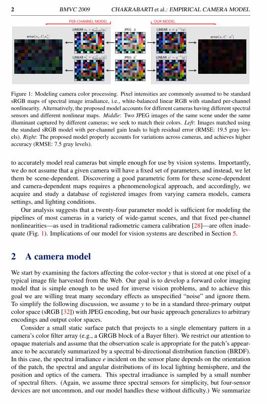
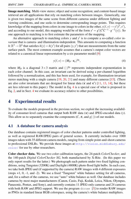
Figure 1: Modeling camera color processing. Pixel intensities are commonly assumed to be standardsRGB maps of spectral image irradiance, i.e., white-balanced linear RGB with standard per-channelnonlinearity. Alternatively, the proposed model accounts for different cameras having different spectralsensors and different nonlinear maps. Middle: Two JPEG images of the same scene under the sameilluminant captured by different cameras; we seek to match their colors. Left: Images matched usingthe standard sRGB model with per-channel gain leads to high residual error (RMSE: 19.5 gray lev-els). Right: The proposed model properly accounts for variations across cameras, and achieves higheraccuracy (RMSE: 7.5 gray levels).

to accurately model real cameras but simple enough for use by vision systems. Importantly,we do not assume that a given camera will have a fixed set of parameters, and instead, we letthem be scene-dependent. Discovering a good parametric form for these scene-dependentand camera-dependent maps requires a phenomenological approach, and accordingly, weacquire and study a database of registered images from varying camera models, camerasettings, and lighting conditions.

Our analysis suggests that a twenty-four parameter model is sufficient for modeling thepipelines of most cameras in a variety of wide-gamut scenes, and that fixed per-channelnonlinearities—as used in traditional radiometric camera calibration [28]—are often inade-quate (Fig. 1). Implications of our model for vision systems are described in Section 5.

2 A camera model

We start by examining the factors affecting the color-vector y that is stored at one pixel of atypical image file harvested from the Web. Our goal is to develop a forward color imagingmodel that is simple enough to be used for inverse vision problems, and to achieve thisgoal we are willing treat many secondary effects as unspecified “noise” and ignore them.To simplify the following discussion, we assume y to be in a standard three-primary outputcolor space (sRGB [32]) with JPEG encoding, but our basic approach generalizes to arbitraryencodings and output color spaces.

Consider a small static surface patch that projects to a single elementary pattern in acamera’s color filter array (e.g., a GRGB block of a Bayer filter). We restrict our attention toopaque materials and assume that the observation scale is appropriate for the patch’s appear-ance to be accurately summarized by a spectral bi-directional distribution function (BRDF).In this case, the spectral irradiance e incident on the sensor plane depends on the orientationof the patch, the spectral and angular distributions of its local lighting hemisphere, and theposition and optics of the camera. This spectral irradiance is sampled by a small numberof spectral filters. (Again, we assume three spectral sensors for simplicity, but four-sensordevices are not uncommon, and our model handles these without difficulty.) We summarize

BMVC 2009 CHAKRABARTI et al.: EMPIRICAL CAMERA MODEL 3

this process asκ(`,v) = π · e(`,v), (1)

where ` represents the spectral and angular distributions of the lighting, v represents theviewing direction and optics, and the operator π represents transmission and sensing throughthe camera’s three spectral filters. We assume this process to be linear, which is justified bythe experimental results in Sect. 4. In an increasing number of digital cameras, the data κ

can be accessed through a RAW output format, and in the sequel, we refer to κ as lineardata because it is linearly related to image irradiance. It is important to remember, however,that Eq. 1 is an approximation to a camera’s RAW output, which may also include the effectsof dark current compensation, flare removal, filling/marking of “dead pixels”, quantization,and noise removal [22, 29]. Here, we consider these as sources of noise and ignore them.

In the next stages of the camera processing pipeline, the linear data κ is used to renderan image in a output color space (sRGB) that is suitable for display purposes [22, 29]. First,there are “pre-processing” operations such as flare and noise removal (if not already done forthe RAW data), white balancing, demosaicing, sharpening, and a linear transformation to aninternal working color space. As above, we model most of these effects as a noise process.One exception is white balance, which we model as a scene-dependent linear transform C.The scene-dependence results from the transform being determined by an “estimated illumi-nant” or “chosen white point” that is output from a computationally-efficient color constancyalgorithm, such as a variant of gray world [3]. The other exception is the color space transfor-mation, which we model as a fixed linear transform that maps three-vectors in the camera’ssensor space (i.e., in terms of the three spectral sensitivities) to colorimetric tristimulus val-ues (say, CIE XYZ) where tone adjustment is applied. Note that a camera’s spectral sensorsare generally not exact linear combinations of the human standard observer’s; so this linearmap is approximate in the sense of producing colorimetric tristimulus values that are slightlydifferent from what the standard observer would have measured in the same scene. (Weevaluate this difference experimentally in Sect. 4.) For notational convenience, we absorbthe fixed linear color-space transform into the white-balance transform C.

The subsequent stage of the pipeline is the most important to our model, and it is alsothe most mysterious. At this stage, the camera modifies the tristimulus values so that they fitwithin the limited gamut and dynamic range of the output color space, and it does so in a waythat is most visually pleasing (as opposed to most accurate). Referred to as color rendering,this is a proprietary art that may include luminance histogram analysis, corrections to hueand saturation, and even local corrections for things such as skin tones. In most cases,this nonlinear color rendering process is scene-dependent and is not a fixed property of acamera. Finally, at the end of the processing pipeline, the rendered image is encoded viare-quantization and compression (usually JPEG), which we again treat as noise and ignore.

Putting this all together, we write the output color vector as

y(`,v) = g(C ·κ(`,v)), (2)

with C ∈ GL(3) as described above, and g: R3→ R3 a nonlinear function. Note that both Cand g depend on global image properties, and that g is a composite of the camera’s scene-dependent color rendering processes and the standard compressive nonlinearity (approxi-mately a “gamma” of 2.2) that is part of the sRGB representation.

The remainder of this paper is devoted to evaluating the accuracy of the model in Eqs. 1and 2. We are particularly interested in developing an efficient representation for the scene-dependent nonlinearity g.

4 BMVC 2009 CHAKRABARTI et al.: EMPIRICAL CAMERA MODEL

3 Applications and related workBefore describing our experiments, it is worth considering the potential utility of the modelwe propose. There are at least three broad categories of applications, and while we do notexplicitly consider these applications in this paper, they influence the form and complexityof the model we develop.

Radiometric calibration. Many vision algorithms require accurate measurements of sceneradiance to succeed; high-dynamic-range imaging, photometric stereo, shape from shad-ing, and reflectometry are but a few examples. For these algorithms to be effective for agiven input y, it is desirable to first “undo” the effects of the nonlinearity by computingx = g−1(y) = C ·κ . If this can be achieved, the resulting image values x are linearly relatedto image irradiance and (assuming one compensates for optical effects like vignetting) sceneradiance, and the algorithms described above can be applied directly.

To accomplish this task, one must have access to a low-parametric model for g as wellas an algorithm for estimating its parameter values from image data. This is similar to theproblem of “grayscale” radiometric calibration [6, 27, 28], which has received significantattention [7, 16, 23, 24, 26]. In fact, our work draws inspiration from Grossberg and Nayar’sempirical study of that problem [17]. In much of this work, it is assumed that the nonlinearity(sometimes called the radiometric response function) is a fixed property of the camera, andin some cases, this has been extended to handle color by computing separate (and fixed)nonlinearities for each color channel (e.g., [23, 28]). For the reasons described above, afixed per-channel nonlinearity is unlikely to accurately model the functions g in Eq. 2 forall images acquired by a given camera. One of the key goals of this paper is to derive afunctional form for g that improves accuracy.

Color constancy. Though it can be formulated in many different ways, the basic goal ofcomputational color constancy is to infer a representation of surface spectral reflectance thatis invariant to changes in the spectral distribution of a scene’s illumination. One approach isto define a “canonical” linear representation of scene color

κo(`o,v) = πo · e(`o,v), (3)

i.e., the color corresponding to a canonical set of spectral sensors πo and canonical illuminant`o (often the equal-energy illuminant E). The goal, then, is to infer κo from a camera’snonlinear output y(`,v) that has been captured under unknown illuminant `.

A common approach is to first calibrate the camera radiometrically, so that x(`,v) =g−1(y(`,v)) = C · κ(`,v) can be computed, and then assume that x(`,v) is related to thedesired canonical representation by a linear (or diagonal) transform: x(`,v) = Mκo, M ∈GL(3) [2, 12, 25, 33]. The transform M depends on the illuminants (`,`o) and sensors (π,πo),and, for any realistic scenario, is a coarse approximation. (The map κo → x is usually notbijective, for example.)

The accuracy of the linear (and diagonal) model x(`,v) = Mκo has been well studiedfor the case of a single camera in a Lambertian world. In this scenario, π = πo, and theconditions for the linear mapping to be accurate can be stated very precisely [4, 10, 34].The problem becomes more complicated when multiple cameras are involved because thespectral filters of the camera cannot be easily related. One of the goals of this paper isto perform an empirical evaluation of the linear model for a broad collection of commoncameras.

BMVC 2009 CHAKRABARTI et al.: EMPIRICAL CAMERA MODEL 5

Image matching. Multi-view stereo; object and scene recognition; and content-based imageretrieval are all applications that rely on matching colors between images. Generically, oneis given two images of the same scene from different cameras under different lighting andviewing conditions, and one seeks to determine corresponding image points. This requiresknowledge of the mapping from colors in one image to colors in the other, y(`,v)→ y′(`′,v′),and according to our model, this mapping would be of the form y′ = g′(C′C−1 ·g−1(y)). Soone approach to matching is to first estimate the parameters of the mapping.

An alternative approach to matching colors y and y′ is to compute a so-called color in-variant that is camera- and illumination-independent. This amounts to computing a functionh: R3→Rk that satisfies h(y) = h(y′) for all pairs (y,y′) that are measurements from the samesurface patch. The most common example assumes that a camera’s output color vectors arerelated to a canonical linear representation by a six-parameter model [9]

y(`,v) = (MD ·κo)γD , (4)

where MD is a diagonal 3×3 matrix and (·)γD represents independent exponentiation ineach color channel. In this case, an invariant can be derived using a per-channel logarithmfollowed by a normalization, and this has been used, for example, for illumination-invariantstereo matching with a single camera [19, 20, 21] and many different cameras [15]. (Thereare also color invariants that are designed for linear data (κ and κ ′) [11, 13, 14], but theseare less relevant to this paper.) The model in Eq. 4 is a special case of what is proposed inEq. 2, and in Sect. 4 we evaluate its accuracy relative to other possibilities.

4 Experimental resultsTo evaluate the models proposed in the previous section, we exploit the increasing availabil-ity of consumer-level cameras that output both RAW data (κ) and JPEG-encoded data (y).This allow us to separately examine the components (C, π , and g(·)) of our models.

4.1 A database for camera analysisOur database contains registered images of color checker patterns under controlled lighting,as well as registered RAW/JPEG pairs of general scenes. It currently includes over 1000images taken with 35 different camera models, ranging from simple point-and-shoot camerasto professional DSLRs. We provide these images at http://vision.middlebury.edu/color/ for use by other researchers.

Color checker data. We use two color calibration targets, the 24-patch ColorChecker, andthe 140-patch Digital ColorChecker SG, both manufactured by X-Rite. (In this paper weonly report results for the latter.) We photograph each pattern under two fixed lighting con-ditions, using Tungsten (3200K) and Daylight (4800K) photo flood light bulbs. In each case,we take both JPEG and (if supported by the camera) RAW images with 4 different exposures(stops +1, 0, -1, and -2). We use a fixed “Tungsten” white balance setting for all cameras,and, for a subset of the cameras, we use “auto” white balance as well. Our database includescameras by most major manufacturers (Canon, Casio, Fuji, Kodak, Leica, Nikon, Olympus,Panasonic, Pentax, and Sony), and currently contains 11 JPEG-only cameras and 24 cameraswith both RAW and JPEG support. We use the program dcraw [5] to render RAW imagesas PNGs in standard linear RGB colorspace, using the camera’s white balance multipliers.

6 BMVC 2009 CHAKRABARTI et al.: EMPIRICAL CAMERA MODEL

In each source image we compute the homography that maps the pattern to a canonicalposition, and resample to obtain cropped and aligned patterns. We generate both point-sampled and “smoothed” (4x linearly down-sampled) versions of these images. The formerrepresent true samples of the original intensities, sensor noise, and JPEG compression ar-tifacts, while the latter (used in the experiments below) attenuate such effects. To removeremaining misregistrations, which are mainly due to lens distortion, we construct our finalregistered images by conservatively cropping the individual color squares of the checkerpattern and compositing them into a single image (see Figure 1 for examples).

This data is sufficient for evaluating the portion of the model (C and g(·)) that relatesRAW data to JPEG data. But in order to evaluate the other portion of the model (π), we mustcompute image irradiance by correcting for optical effects (vignetting) and spatial variationsin the incident illumination. We do this by fitting 2D spatial gain functions over the registeredpatterns, composed of a linear function per illuminant and a quadratic radial function percamera. These gain functions are estimated using the gray patches around the perimeter ofthe color checker, and they correct the spatial variations of the aligned RAW images to aresidual non-uniformity of less than 3%. These “spatially-corrected” images can then bedirectly compared to the known relative radiance values of the color checker squares.

General scenes. A subset of the RAW-capable cameras in our database allow simultaneouscapture of RAW/JPEG pairs, and with these devices we can capture registered pairs in naturalenvironments. Our database includes a total of 85 such pairs taken of general indoor andoutdoor scenes with 12 different camera models. We use these images in Sect. 4.3.

4.2 Camera sensor characteristics

We first evaluate the validity of Eq. 1 by exploring the relationship between spectral imageirradiance and cameras’ sensor measurements. We are interested in assessing the degree towhich output RAW values are linearly related to image irradiance, as well as understandingthe nature of each camera’s spectral filters π . For these experiments, we use a canonicallinear representation κ0 of the color checker (provided by the manufacturer) consisting ofCIE XYZ values under illuminant D65, and we compare these to the spatially-correctedRAW images described above.

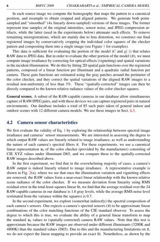
In the first experiment, we find that in the overwhelming majority of cases, a camera’sRAW output is indeed linearly related to image irradiance. A representative example isshown in Fig. 2(a), where we see that once the illumination variation and vignetting effectsare removed, the RAW values form a near-exact linear relationship with the known relativescene radiance of the color checker. If we measure deviation from linearity using RMSresidual error in the total-least-squares linear fit, we find that the average residual over the 24RAW-capable cameras in our database is 1.6 gray levels, while the average RMS noise level(estimated from the variance within the squares) is 0.7.

In the second experiment, we explore (somewhat indirectly) the spectral composition ofeach camera’s sensors. One expects a camera’s spectral sensors (π) to be approximate linearcombinations of the color matching functions of the CIE standard observer. To assess thedegree to which this is true, we evaluate the ability of a general linear transform to mapthe standard κ0 values to (spatially-corrected) camera RAW values. Note that this test isapproximate because the RAW images are observed under different illuminants (3200K and4800K) than the standard values (D65). Due to this and the manufacturing limitations on π ,we do not expect the linear mapping to provide an exact fit. Nonetheless, as shown by the

BMVC 2009 CHAKRABARTI et al.: EMPIRICAL CAMERA MODEL 7

Can

onE

OS

20D

RA

W

Tran

sfor

med

XY

Zun

derD

65

Tran

sfor

med

XY

Zun

derD

65

Relative radiance of gray patches Panasonic LX3 RAW under 3200K Panasonic LX3 RAW under 4800K

(a) (b) (c)

Figure 2: (a) Camera RAW vs. image irradiance. The plot shows a typical, almost perfectly linearrelationship between a camera’s RAW output (Canon EOS 20D) and relative scene radiance, as givenby the 14 unique gray squares of a color checker. (b, c) Typical joint intensity histograms for CameraRAW and CIE XYZ, showing that a general 3x3 linear transform can provide a reasonable fit. Shownare the joint histograms comparing the RAW intensities of a Panasonic LX3 camera under two differentilluminants (b) 3200K, and (c) 4800K, with the best C-transformed color checker CIE XYZ valuesunder Illuminant D65.

representative examples in Fig. 2(b,c), the linear transform does a reasonable job for most ofthe cameras and illuminants in our database. The average RMS residual error in this case is2.76 gray levels over all RAW images—approximately four times the noise level.

4.3 Nonlinear processing

Next, we evaluate three different models, composed of C ∈ GL(3) and g: R3→ R3, for thecameras’ color rendering pipelines. These models increase in complexity.

1. Independent exponentiation. Recent work has considered the model of Eq. 4 for casesin which the per-channel exponents are equal and known [15], equal and unknown [19,20], and arbitrary [9]. We generalize these by replacing the diagonal transform by ageneral linear transform and allowing the exponents to be arbitrary. The resultingmodel is y = (C ·κ)γD , and it has 12 parameters (9 for the entries of C, and 3 for γD).

2. Independent polynomial. A more general model is obtained by replacing the per-channel exponential by an nth-degree polynomial. This is partially motivated by thesuccess of polynomial model for traditional “per-channel” radiometric calibration [23,28]. We write our model as yi = gi([C · κ]i) where yi is the value of the ith colorchannel, and gi(x) = ∑

np=0 βi,pxp is constrained to be monotonic in the typical range

of x. Note that the scale of each column of C can be absorbed into the correspondingpolynomial, so the total number of parameters in this model is 3(n+3).

3. General polynomial. More general than restricting the nonlinearity to operate inde-pendently in each C-transformed color channel is to consider an nth-degree polyno-mial map from R3 to R3. This is written yi = ∑p1+p2+p3≤n βi,p1 p2 p3 κ

p11 κ

p22 κ

p33 , with

parameters {βi,p1 p2 p3} that capture both the effect of the linear transform C and thenonlinearity. The total number of parameters in this model is considerably larger at12 (n+1)(n+2)(n+3).

8 BMVC 2009 CHAKRABARTI et al.: EMPIRICAL CAMERA MODELR

MS

Err

or

2 4 6 80

5

10

15

20

25

Independent ExponentiationIndependent PolynomialGeneral Polynomial

Polynomial Degree

RM

SE

rror

2 4 6 80

2

4

6

8

Independent ExponentiationIndependent PolynomialGeneral Polynomial

Polynomial Degree

(a) (b) (c) (d)

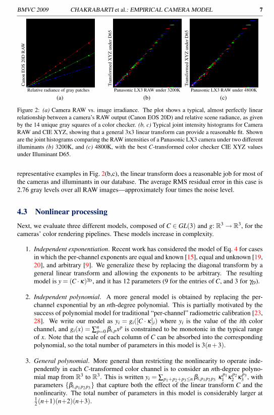
Figure 3: RAW→JPEG maps using different models for general scenes. (a) Plot of residual RMS errorfor different models, (b) JPEG from camera, (c) JPEG fitted from RAW images using independentpolynomial model with n = 5, and (d) Absolute error value image (scaled up by 10 for visibility).Note that most errors occur in high-frequency regions where we also expect unmodeled errors due tosharpening and compression.

These models are evaluated by estimating parameters for the best least-squares fit be-tween a number of RAW/JPEG pairs—each pair providing a set of (κ,y) pairs. We measurethe quality of the fit by reporting the root-mean-squared-error (RMSE) over the training set.For the independent exponentiation model, simple regression is used to find the optimal Ccorresponding to every choice of γD, and the optimal γD is determined by exhaustive searchin a large range of possible values. The parameters for the general polynomial model can beestimated with simple regression as well.

For the independent polynomial model an iterative approach is needed. Given an estimateof C, we compute the parameters of the gi(·) functions using quadratic programming tominimize the least-squares error with monotonicity constraints. Then, C is updated with astep along the error gradient, which is computed assuming fixed gi(·). We choose our initialestimate for C such that the [C ·κ]i-values corresponding to the same yi in the training set{κk,yk}K

k=1 are close to being equal: We partition the domain of yi into a finite set of valuesV. For each v ∈ V, a weight vector wvi ∈ RK measures the “membership” of every yk,i tothe partition corresponding to v (we use wvi

k = exp(−λ (yk,i− v)2)). The ith row cTi of C is

computed to minimize the weighted variance Si = cTi Aici with Ai ∈ R3×3 defined as

Ai = ∑v∈V

K

∑k=1

wvik

(xvi

k xvik

T)

, with xvik = κk−

∑k wvik κk

∑k wvik

. (5)

The nontrivial solution for ci is the smallest eigenvector of Ai.Figure 3(a) shows the typical performance of the models when applied to RAW/JPEG

pairs of natural scenes. The independent exponentiation model is the simplest and performsworse than polynomial models with degree greater than two. The general polynomial modelprovides only a marginal benefit over independent polynomial model, even though it has amuch larger number of parameters. Based on these results, we settle on the independentpolynomial model with degree n = 5 as a good balance between accuracy and complexity,and we use this model for the remainder of the paper. Figures 3(b-d) compare the true JPEGsand corresponding mapped RAW images using this 24-parameter model.

Having settled on the independent polynomial model with n = 5, we next explore thismodel more systematically using the color checker images. Since the color checker provides

BMVC 2009 CHAKRABARTI et al.: EMPIRICAL CAMERA MODEL 9

0 2 4 6 8 10 12

CanonPowerShotG1

CanonPowerShotS60

SonyDSC−F828

CasioEX−Z55

CanonPowerShotS50

NikonD3

CanonPowerShotG9

CanonPowerShotG10

PanasonicDMCLX3

CanonEOSDigitalRebelXSi

CanonEOS1DsMarkII

NikonD70

CanonEOS20D

CanonEOSDigitalRebel

FujifilmFinePixS5Pro

OlympusE10

NikonD200

LeicaM8

PentaxK10D

NikonD300

SonyDSLR−A100

CanonEOS5D

SonyDSLR−A300

OlympusE500 Mean Noise Std. Dev.

Mean RMSE

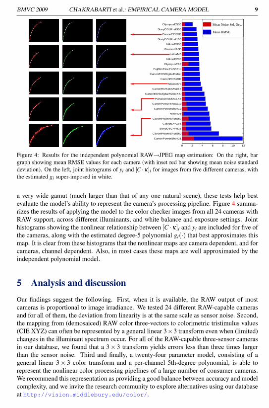
Figure 4: Results for the independent polynomial RAW→JPEG map estimation: On the right, bargraph showing mean RMSE values for each camera (with inset red bar showing mean noise standarddeviation). On the left, joint histograms of yi and [C ·κ]i for images from five different cameras, withthe estimated gi super-imposed in white.

a very wide gamut (much larger than that of any one natural scene), these tests help bestevaluate the model’s ability to represent the camera’s processing pipeline. Figure 4 summa-rizes the results of applying the model to the color checker images from all 24 cameras withRAW support, across different illuminants, and white balance and exposure settings. Jointhistograms showing the nonlinear relationship between [C ·κ]i and yi are included for five ofthe cameras, along with the estimated degree-5 polynomial gi(·) that best approximates thismap. It is clear from these histograms that the nonlinear maps are camera dependent, and forcameras, channel dependent. Also, in most cases these maps are well approximated by theindependent polynomial model.

5 Analysis and discussion

Our findings suggest the following. First, when it is available, the RAW output of mostcameras is proportional to image irradiance. We tested 24 different RAW-capable camerasand for all of them, the deviation from linearity is at the same scale as sensor noise. Second,the mapping from (demosaiced) RAW color three-vectors to colorimetric tristimulus values(CIE XYZ) can often be represented by a general linear 3×3 transform even when (limited)changes in the illuminant spectrum occur. For all of the RAW-capable three-sensor camerasin our database, we found that a 3× 3 transform yields errors less than three times largerthan the sensor noise. Third and finally, a twenty-four parameter model, consisting of ageneral linear 3× 3 color transform and a per-channel 5th-degree polynomial, is able torepresent the nonlinear color processing pipelines of a large number of consumer cameras.We recommend this representation as providing a good balance between accuracy and modelcomplexity, and we invite the research community to explore alternatives using our databaseat http://vision.middlebury.edu/color/.

10 BMVC 2009 CHAKRABARTI et al.: EMPIRICAL CAMERA MODEL

The next step is to explore applications of such a model to visual tasks such as colorconstancy, radiometric calibration, and image matching. Here, the goal will be to estimatethe model parameters from natural input image data. We view the image matching problemas particularly interesting because it is likely that matching image patches y(`,v)↔ y′(`′,v′)can be achieved through a “shortcut” model y = g(y′) or through the use of invariants thatdo not require estimating a full set of parameters for each camera. It may also be possible toisolate local image effects, such as specular highlights and shading changes, from the globalimage differences caused by camera-dependent color processing.

In order to fully exploit the Internet as a data source for computer vision, we must usethe color information that is available in its images. Doing so requires compensating for thescene-dependent nonlinear color processing performed by consumer cameras, and derivingmodels like those proposed here is an important first step in this direction.

Acknowledgments

Many thanks to Porter Westling for his help in creating the image database used in this paper.Support for AC and TZ was provided by NSF Career Award IIS-0546408, ARO grant 54262-CI, and a fellowship from the Alfred P. Sloan Foundation. Support for DS was provided byNSF grants IIS-0413169 and IIS-0713442.

References[1] T. Berg, A. Berg, J. Edwards, M. Maire, R. White, Y. Teh, E. Learned-Miller, and D. Forsyth.

Names and faces in the news. In Proc. IEEE Conf. Computer Vision and Pattern Recognition,pages 848–854, 2004.

[2] D. Brainard and W. Freeman. Bayesian color constancy. J. Optical Society America A, 14(7):1393–1411, 1993.

[3] G. Buchsbaum. A spatial processor model for object colour perception. J. Franklin Institute, 310(1):1–26, 1980.

[4] H. Chong, S. Gortler, and T. Zickler. The von Kries hypothesis and a basis for color constancy.In Proc. IEEE Intl. Conf. Computer Vision, 2007.

[5] dcraw. Decoding raw digital photos in Linux. http://www.cybercom.net/~dcoffin/dcraw/, Last accessed: July 29, 2009.

[6] P. Debevec and J. Malik. Recovering high dynamic range radiance maps from photographs. InSIGGRAPH ’97: Proc. Conf. Computer Graphics, pages 369–378, 1997.

[7] H. Farid. Blind inverse gamma correction. IEEE Trans. Image Processing, 10(10):1428–1433,2001.

[8] R. Fergus, P. Perona, and A. Zisserman. A visual category filter for Google images. In Proc.European Conf. Computer Vision, pages 242–256, 2004.

[9] G. Finlayson and R. Xu. Illuminant and gamma comprehensive normalisation in log RGB space.Pattern Recognition Letters, 24(11):1679–1690, 2003.

[10] G. Finlayson, M. Drew, and B. Funt. Color constancy: generalized diagonal transforms suffice.J. Optical Society America A, 11(11):3011–3019, 1994.

[11] G. Finlayson, S. Hordley, and M. Drew. Removing shadows from images. In Proc. EuropeanConf. Computer Vision, pages 823–836, 2002.

[12] D. Forsyth. A novel algorithm for color constancy. Intl. J. Computer Vision, 5(1), 1990.

BMVC 2009 CHAKRABARTI et al.: EMPIRICAL CAMERA MODEL 11

[13] J. Geusebroek, R. Van den Boomgaard, A. Smeulders, and H. Geerts. Color invariance. IEEETrans. Pattern Analysis and Machine Intelligence, 23(12):1338–1350, 2001.

[14] T. Gevers and A. Smeulders. Color-based object recognition. Pattern recognition, 32(3):453–464,1999.

[15] M. Goesele, N. Snavely, B. Curless, H. Hoppe, and S. Seitz. Multi-view stereo for communityphoto collections. In Proc. IEEE Intl. Conf. Computer Vision, 2007.

[16] M. Grossberg and S. Nayar. Determining the camera response from images: what is knowable?IEEE Trans. Pattern Analysis and Machine Intelligence, 25(11):1455–1467, 2003.

[17] M. Grossberg and S. Nayar. Modeling the space of camera response functions. IEEE Trans.Pattern Analysis and Machine Intelligence, 26(10):1272–1282, 2004.

[18] J. Hays and A. Efros. IM2GPS: estimating geographic information from a single image. In Proc.IEEE Conf. Computer Vision and Pattern Recognition, 2008.

[19] Y. Heo, K. Lee, and S. Lee. Illumination and camera invariant stereo matching. In Proc. IEEEConf. Computer Vision and Pattern Recognition, 2008.

[20] Y. Heo, K. Lee, and S. Lee. Mutual information-based stereo matching combined with SIFTdescriptor in log-chromaticity color space. In Proc. IEEE Conf. Computer Vision and PatternRecognition, 2009.

[21] H. Hirschmüller and D. Scharstein. Evaluation of stereo matching costs on images with radio-metric differences. IEEE Trans. Pattern Analysis and Machine Intelligence, 2009.

[22] J. Holm, I. Tastl, L. Hanlon, and P. Hubel. Color processing for digital photography. In P. Greenand L. MacDonald, editors, Colour Engineering: Achieving Device Independent Colour, pages179–220. Wiley, 2002.

[23] S. Kuthirummal, A. Agarwala, D. Goldman, and S. Nayar. Priors for large photo collections andwhat they reveal about cameras. In Proc. European Conf. Computer Vision, 2008.

[24] S. Lin, J. Gu, S. Yamazaki, and H.-Y. Shum. Radiometric calibration from a single image. InProc. IEEE Conf. Computer Vision and Pattern Recognition, 2004.

[25] L. Maloney and B. Wandell. Color constancy: a method for recovering surface spectral re-flectance. J. Optical Society America A, 3(1):29–33, 1986.

[26] C. Manders, C. Aimone, and S. Mann. Camera response function recovery from different illumi-nations of identical subject matter. In Proc. Intl. Conf. Image Processing, volume 5, 2004.

[27] S. Mann and R. Picard. Being ‘undigital’ with digital cameras: Extending dynamic range bycombining differently exposed pictures. In Proc. IS&T Annual Conf., pages 422–428, 1995.

[28] T. Mitsunaga and S. Nayar. Radiometric self calibration. In Proc. IEEE Conf. Computer Visionand Pattern Recognition, 1999.

[29] R. Ramanath, W. Snyder, Y. Yoo, and M. Drew. Color image processing pipeline. IEEE SignalProcessing Magazine, 22(1):34–43, 2005.

[30] B. Russell, A. Torralba, K. Murphy, and W. Freeman. LabelMe: a database and web-based toolfor image annotation. Intl. J. Computer Vision, 77(1):157–173, 2008.

[31] N. Snavely, S. Seitz, and R. Szeliski. Photo tourism: Exploring photo collections in 3D. ACMTrans. Graphics (Proc. SIGGRAPH), 3(25):835–846, 2006.

[32] M. Stokes, M. Anderson, S. Chandrasekar, and R. Motta. A standard default color space forthe internet: sRGB. Microsoft and Hewlett-Packard Joint Report, Version 1.10. Available athttp://www.color.org/sRGB.xalter., 1996.

[33] J. van de Weijer, T. Gevers, and A. Gijsenij. Edge-Based Color Constancy. IEEE Trans. ImageProcessing, 16(9):2207–2214, 2007.

[34] G. West and M. Brill. Necessary and sufficient conditions for von Kries chromatic adaptation togive color constancy. J. Math. Bio., 15(2):249–258, 1982.