The Nature of Market Selection in Colombia:

Have Market Reforms Changed the Evolution of

Productivity and Profitability?∗

Marcela Eslava, John Haltiwanger, Adriana Kugler and Maurice Kugler†

November 7, 2003

Abstract

Healthy market economies are continually undergoing productivity en-hancing reallocation. Estimates for the U.S. suggest that in some sectorsthis productivity enhancing reallocation is the dominant factor in account-ing for producitivity growth. An open question, especially for develop-ing countries, is whether reallocation is always productivity enhancing.It may be, for example, that imperfect competition or other barriers tocompetitive environments imply that the reallocation process is not fullyefficient. Using a unique plant-level longitudinal dataset for Colombiafor the period 1982-1998, we explore these issues by examining the roleof productivity and demand in determining plant exits. Moreover, giventhe important trade, labor and financial market reforms in Colombia dur-ing the early 1990’s, we explore whether and how the reallocation processchanged over the period of study. Our data permits measurement ofplant-level quantities and prices. We can estimate total factor productiv-ity (TFP) with plant-level physical output data, where we use downstreamdemand to instrument inputs. In turn, we can estimate demand shocksand mark-ups with plant-level price data, using TFP to instrument foroutput in the inverse-demand equation. Consistent with vintage capitalmodels, our results show that entering businesses are more productive andexiting businesses are less productive than incumbents. In addition, wefind that both lower productivity and lower demand contribute to weedout businesses out of the market, and greater importance of both the pro-ductivity and demand components of profitability following the reforms.

∗We thank Alberto Serrano and Juan Manuel Contreras for excellent research assistance,Alvaro Suarez and Jose Eduardo Granados at DANE for providing access to data, the staff incharge of the AMS for answering our queries on methodological issues regarding the data, andparticipants at various seminars at DANE for their comments and suggestions. Support forthis project was provided by the World Bank. John Haltiwanger also acknowledges financialsupport from the NSF and the IDB, Adriana Kugler from the Spanish Ministry of Scienceand Technology through grant No. SEC-2000-1034, and Maurice Kugler from the IDB.

†Marcela Eslava: University of Maryland, e-mail: eslava@econ.umd.edu. John Halti-wanger: University of Maryland and NBER, e-mail: haltiwan@econ.umd.edu. Adriana Ku-gler: University of Houston, CEPR and IZA, e-mail: adkugler@uh.edu. Maurice Kugler:University of Southampton and GEP, e-mail: maurice.kugler@soton.ac.uk.

1

1 Introduction

Market economies are continually restructuring in response to changing condi-tions. The burgeoning evidence from longitudinal micro business databases hasshown that productivity growth at the aggregate level is closely connected tothe efficiency of the economy at the micro level to allocate outputs and inputsacross businesses. That is, a large fraction of measured productivity growth isaccounted for by more productive entering and expanding businesses displacingless productive exiting and contracting businesses.1

Understanding of these issues has hardly been settled in advanced economiesbut these issues loom especially large in developing economies. In developingeconomies, there are potentially a variety of barriers to promoting efficient ongo-ing reallocation. These barriers might stem from distortions in market structureas well as the market institutions and policies in place. Aware of the impedi-ments that distortionary policies may place on reallocation and, more generally,on productivity growth, during the past decade Latin American countries haveundertaken a whole series of reforms (including, labor, financial, and trade re-forms) to promote flexibility.In this paper, we examine how reallocation contributes to productivity and

also to profitability in one Latin American country, Colombia. We, then, askhow the relation between reallocation and productivity and profitability changedafter market reforms were introduced in Colombia in the early 1990’s. Colombiais a superb country to study these issues for two reasons. First, Colombiaunderwent a substantial and relatively fast market reform process, maily in 1990and 1991. The 1990 labor market reform, which introduced individual severancepayments savings accounts, reduced dismissal costs by about 50% (Kugler (1999,2002)). The 1991 trade liberalization reduced the average tariff from over 62%to around 15% (Lora (1997)). The financial reform first introduced in 1990and extended in 1991, liberalized deposit rates, eliminated credit subsidies andmodernized capital market and banking legislation (Lora (1997)). In addition,restrictions on inflows of foreign direct investment were removed in 1991 (Kugler(2000)). The 1993 social security reform allowed voluntary transfers from a pay-as-you-go system to a fully-funded system with individual accounts, thought itincreased employer and employee pension contributions up to 13.5% of earnings(Kugler and Kugler (2003)).Second, Colombia has unique longitudinal microeconomic data on busi-

nesses. The unique feature of the Colombian data is that both plant-levelquantities and prices can be measured. The ability to measure plant-levelprices of both outputs and inputs is potentially very important in this contextfor both measurement and conceptual reasons. Much of the existing literaturemeasures establishment output as revenue divided by a common industry-leveldeflator. Therefore, within-industry price differences are embodied in outputand productivity measures. If prices reflect idiosyncratic demand shifts or mar-

1For the labor market, the efficient churning of businesses implies a need to reallocate jobsat a high pace without long and costly spells of unemployment. The latter is important fornot only productive efficiency of the economy but also obviously important for welfare.

2

ket power variation rather than quality or production efficiency differences, thenhigh measured “productivity” businesses may not be particularly efficient. Ifthis is the case, then what the empirical literature has been documenting asselection on productivity is really selection on profits.2 In this sense, the re-lation between productivity and survival probability, reallocation, and industrydynamics may be overstated.3

In the context of a developing economy undergoing structural reforms thesemeasurement and conceptual issues are especially important. A key objectiveof market reforms is to make markets more competitive. Without the ability tomeasure plant-level prices it is very difficult to measure and, in turn, analyzethe respective contributions of demand and efficiency factors in market selectionand how they may have changed in response to market reforms. In this paper,we attempt to measure the separate influences of idiosyncratic productivity anddemand on market selection in Colombia.In exploiting these unique micro data, our paper makes a number of re-

lated methodological innovations relative to much of the literature. First, inmeasuring efficiency we estimate production functions using an extension of theinstrumental variable approach pioneered by Syverson (2003). In the latter,Syverson uses local downstream demand instruments to estimate returns toscale of production functions. Building on this approach, we use downstreamdemand instruments as well as plant-level input prices for materials and energyas instruments in estimating production functions. From this structural estima-tion of production functions, we generate measures of plant-level efficiency (i.e.,plant-level total factor productivity). Second, since we can measure plant-leveloutput prices, we estimate demand elasticities using the total factor produc-tivity estimates as instruments in the demand equations. That is, we first usedownstream demand instruments to estimate production functions and then usesupply shocks (i.e., total factor productivity) to estimate the demand functions.Having estimated production and demand functions, we study the evolu-

tion of the distributions of total factor productivity, prices and demand shocksthrough the market reforms in Colombia. Our focus is on the market selectiondynamics in Colombia throughout the entire period as well as during periods

2Profitability will depend on several factors: efficiency, input prices, demand and poten-tially other factors including government subsidies and taxes. In what follows, we estimateand take advantage of some of these key components: idiosyncratic variation in efficiency(TFP), demand and some input prices (in particular, materials and energy). Unobservedcomponents of idiosyncratic profitability are part of the error terms in our market selectionequations and, interestingly, the idiosyncratic unobserved components likely have changed inresponse to market reforms.

3Since Marschak and Andrews (1944), there has been awareness about the possible difficul-ties involved in using revenue-based deflated output in establishment level data. Klette andGriliches (1996) consider how intra-industry price fluctuations can affect production functionand productivity estimates. Melitz (2000) explores this problem further and extends the anal-ysis to consideration of multi-product producers. Katayama, Lu, and Tybout (2003) arguethat both revenue-based output and expenditure-based input measures can lead to productiv-ity mismeasurement and incorrect interpretations about how heterogeneous producers respondto shocks and the associated welfare implications. Foster, Haltiwanger and Syverson (2003)use plant-level data on quantities and prices for the U.S. to study market selection dynamics.

3

prior to and subsequent to the reforms. Overall, we find that market selectionis productivity enhancing but also reflects demand-side factors in Colombia.That is, businesses that exit are less efficient and face higher costs than in-cumbents but also face lower demand for their products relative to incumbents.Entering businesses are more efficient than incumbents and exiting businesses,but also face lower demand relative to incumbents. This finding points to theimportance of vintage technology rather than learning to account for produc-tivity dynamics. Consistent with these patterns, we find that the probability ofexiting decreases with both the efficiency and demand for the products of thebusiness.4 Note that revenue-based TFP measures spuriously include a demandcomponent and thus underestimate technical efficiency of entrants, who have tobuild a consumer base, relative to incumbents, who have a established clien-tele. Hence, the analysis in the present paper provides a better basis to discernbetween vintage and learning explanations for dynamics and heterogeneity inproductivity.How did these patterns change in response to the market reforms? After

the market reforms, the positive gap between the productive efficiency of theaverage incumbent and the average exiting business rises but the positive gapbetween the productive efficiency of the average entering business and the aver-age incumbent declines. On net, the contribution of entry and exit to averageproductivity rises slightly. Moreover, when we investigate a more dynamic spec-ification we find patterns consistent with learning and selection effects that in-crease the contribution of net entry. That is, after market reforms, we find thatsurviving entrants exhibit more rapid productivity growth than incumbents.Putting these pieces together suggests market reforms yielded a more heteroge-nous group of entrants but that conditional on survival the post-market reformentrants contribute more to productivity growth. Increased learning after thereforms may be due to increased access to new imported capital vintages andincreased access to know-how from foreign businesses. In addition, we find thatthe contribution of productivity and demand in accounting for the likelihoodof exit increases after the reforms. These patterns are consistent with greatermarket discipline weeding the least productive and unprofitable businesses outthe market due to increased foreign competition, less access to subsidized credit,and lower dismissal costs.Before proceeding, it is useful to emphasize that the welfare implications

(and even the productivity implications) are complex in this context with im-perfect competition. Our paper is intended to be a contribution on charac-terizing the positive implications of market reform rather than the normativeimplications. There are several interesting complicating factors in consideringwelfare implications. For one, the market power of firms may derive from eco-nomic fundamentals or from institutional factors. For example, it may be thatmarket power derives from product differentiation by each producer and that

4We also find that businesses with higher input costs (in terms of materials and energy) aremore likely to exit. In this version we use the input prices essentially as controls but plan toinvestigate the relationship between market reforms, market selection and input prices morefully in future drafts.

4

markets are best characterized by monopolistic competition. The exploitationof market power in this context by firms still generates a welfare loss with pricesbeing above marginal cost, but even in the absence of markups substantial priceheterogeneity across firms would still be a feature of a first best equilibrium.Alternatively (or in addition), market power may derive from institutional bar-riers (e.g., trade restrictions). Simple intuition suggests that elimination ofsuch barriers will improve welfare, but even here one should be cautious givenpotential second best considerations. Another related complicated factor isthat market power may play an important role in product and process innova-tions that lead to technological progress. In some creative-destruction modelsof innovation and growth (e.g., Aghion and Howitt (1992)), market power playsan important role for innovators in an environment in which there are fixedcosts of innovation. We do not have much to say directly about this latter classof models since we do not directly investigate the role of product and processinnovation. Part of the reason for this is that our empirical focus is on oper-ating plants in manufacturing (not R&D facilities). Our analysis has more tosay about adoption issues (e.g., in vintage models of technological adoption, itis the new plants that adopt the new technology) than innovation. However, along standing issue in the empirical innovation literature is how much innovationoccurs in R&D facilities and how much occurs on the factory floor.The rest of the paper proceeds as follows. Section 2 describes the Colom-

bian context and the market reforms undertaken during the period of study.Section 3 describes the unique data we use. Section 4 presents results of theestimation of plant-level total factor productivity and demand shocks. Section5 describes basic patterns of productivity, demand, and prices in terms of dis-persion, persistence, and cyclicality, and also contrasts the patterns of entering,continuing and exiting plants. Section 6 examines the contribution of efficiencyand demand on exit probabilities. Section 7 concludes.

2 Market Reforms in Colombia

In 1990, the administration of President Cesar Gaviria conceived a compre-hensive reform package, which included not only measures to modernize thestate and liberalize markets but also a constitutional reform. In contrast tothe experience in many reformist countries, there was no underlying economiccrisis preceding the reform in Colombia. Rather, ample social and politicalunrest were the catalysts for institutional change (see, e.g., Edwards (2001)).Structural reforms to remove distortions from product and factor markets wereintroduced in parallel with constitutional changes to political institutions aspart of a wider effort to control internal strife associated with violent activitiesof both illicit drug cartels and guerrilla groups. The absence of an economiccrisis meant that there was no clear consensus for the need of market-orientedreforms, but at the same time good economic conditions were an asset as dis-tributive conflict was addressed by elaborate compensation schemes (see, e.g.Kugler and Rosenthal (2003)). However, the inability to continue redistribut-

5

ing meant that by 1993 the spurt of reform of the early nineties came to a halt.Although there was no reversal of reforms, Colombia did not make additionalprogress in terms of further removing distortions while many other countriesin Latin America, and around the world, actually deepened reform efforts (see,e.g., Burki and Perry (1997)). The fact that structural reform in Colombiawas a one-off phenomenon aids our identification strategy in trying to assess itsimpact on market selection.Before Gaviria’s administration, the government of President Virgilio Barco

made some partial progress in trade liberalization but did not gain any signif-icant ground in removing other distortions. The gradual decrease in tariffsinitiated by Barco was accelerated by Gaviria after June 1991. By the end of1991, nominal protection reached 14.4% and effective protection 26.6%, downfrom 62.5% a year earlier, and 99.9% of items were in the free import regime.These measures clearly generated unrest among the owners of capital, who facedlower profit margins after trade liberalization due to increased foreign competi-tion. The impact from market penetration by foreign exporters, and investorsas pointed out below, on the market participation of domestic businesses inproduct markets was mitigated by more favorable conditions in factor markets.In labor markets, Law 50 of December 1990 promoted the flexibilization of con-tracts and reduced labor costs (see, e.g., Kugler (1999, 2002)). For example, thereform reduced dismissal costs of an employee with 10 years of experience by 56% - under the old legislation the worker had the right to 30.8 monthly salaries,under the new one this was reduced to 13.5. In 1990, the government also triedto introduce changes in the social security system as part of the labor reformpackage, but Congress forced an independent process to reform pension provi-sion. Later during the Gaviria administration, the executive compromised withCongress by passing Law 100 in 1993. Although Law 100 allowed for voluntaryindividual conversion from a pay-as-you-go system to a fully-funded system withaccounts, this law also introduced a mandatory hike in employer and employeecontributions up to 13.5% of salaries, of which 75% was paid by employers (see,e.g., Kugler and Kugler (2003)).A number of measures also reduced frictions in financial markets. In 1990,

Law 45 was introduced with the goal of reducing state control and ownershipconcentration in the banking sector. Interest rate ceilings were eliminated andrequirement reserves were reduced. At the same time, supervision was rein-forced in line with the Basle Accords for capitalization requirements, thoughthere were no requirements for banks to invest in government securities. Law 9of 1991 established the abolition of exchange controls eliminating the monopolyof the central bank on foreign exchange transactions and lowering substantiallythe extent of capital controls. Finally, Resolution 49 of 1991 eliminated re-strictions to foreign direct investment. This resolution established nationaltreatment of foreign enterprises and eliminated limits on the transfer of profitsabroad as well as bureaucratic procedures requiring the approval of individualprojects (see, e.g., Kugler (2000)). This measure not only facilitated capitalinflows across all sectors, but also induced entry of foreign banks increasingcompetition in financial intermediation.

6

After the end of Gaviria’s term, in 1994 President Ernesto Samper gainedpower on a platform partially based on opposition to market institutions.5

While the new government was unsuccessful in terms of dismantling existingreforms, the coalition supporting the new government managed to bring themomentum for additional reforms to a halt. Overall, though, the reform pro-cess was relatively smooth and successful in transforming a highly distortedeconomy into one burdened with many fewer frictions. If the goal of induc-ing productivity-enhancing reallocation was achieved, it should be reflected indifferent patterns of industrial dynamics between the 1980’s and the 1990’s.

3 Data Description

Our data comes from the Colombian Annual Manufacturers Survey (AMS) forthe years 1982 to 1998. The AMS is an unbalanced panel of Colombian plantswith more than 10 employees, or sales above a certain limit (around US$35,000in 1998). The unbalanced nature of the panel allows to distinguish industrydynamics among continuing, entering and exiting plants.6 The AMS includesinformation for each plant on: value of total output and prices charged for eachproduct manufactured; total cost and prices paid for each material used theproduction process; energy consumption in physical units and energy prices;production and non-production worker employment and payroll; and book val-ues of equipment and structures. The dataset also provides information onplant location as well as industry classification codes (5 digits CIIU).Our aim in this paper is to document the evolution of productivity and

demand shocks in the Colombian context and to examine the impact of theseshocks on plants’ exit decisions. To this end, we estimate total factor productiv-ity (TFP) values for each plant using a capital-labor-materials-energy (KLEM)production function and demand shock values for each plant using a standardinverse-demand function. To estimate production and inverse-demand equa-tions, we need to construct physical quantities and prices of output and inputs.With the rich information on prices collected in the AMS, we can construct

plant-level price indices for output, materials, and energy. This represents anenormous advantage with respect to other sources of data, as the use of moreaggregate price deflators is a common source of measurement error. Pricesof output and materials are constructed using Tornqvist indices. Tornqvistindices for a composite of products or materials i of each plant j at time tare constructed by taking the weighted average of the growth in prices for all

5Note that the Colombian electoral system rules out re-election.6The fact that the AMS only samples plants with more than 10 employees or production

above a certain threshold, however, implies that we cannot distinguish between plants whichenter the market and plants which enter the sample because they transition from being less-than-10-employee plants to being more-than-10-employee plants or plants which transitionfrom being below to being above the production threshold. Similarly, we cannot distinguishbetween plants which exit the market and plants which stop being sampled because theytransition from being more-than-10-employee plants to being less-than-10-employee plants, orplants which transition from being above to being below the sales threshold.

7

products or materials h generated by the plant and constructing an index basedon this yearly growth, using 1982 as the base year. The weighted average ofthe growth of prices for all products or materials h produced by plant j at timet is:

∆Pijt =HXh=1

sht∆ ln(Pht),

where i = Y,M, i.e., output or materials,

∆ ln(Pht) = lnPht+1 − lnPht,and

sht =sht + sht+1

2

and Pht and Pht+1 are the prices charged for product h, or paid for materialh, at time t and t + 1, and sht and sht+1 are the shares of product h in plantj’s total production for year t, or the shares of material h in the total value ofmaterials’ purchases for years t and t+1.7 The indices for the levels of output(or material) prices for each plant j are then constructed using the weightedaverage of the growth of prices and fixing 1982 as the base year:

lnPjt = lnPijt−1 +∆Pijt

for t > 1982, where Pj1982 = 100, and where the price levels are then simplyobtained by applying an exponential function to the natural log of prices, Pijt =explnPijt .8

Given prices for materials and output, the quantities of materials and outputare constructed by dividing the cost of materials and value of output by thecorresponding prices. Quantities of energy consumption are directly reported bythe plant. In addition, we need capital stocks to estimate a KLEM productionfunction. We use the nominal capital stock directly reported by the plant ineach year, but correcting the series for each plant to make them consistent overtime.9 In particular, we subtract the inflation adjustment component that was

7The distribution of the weighted average of the growth of prices has large outliers, espe-cially at the left side of the distribution. In particular, the distribution shows negative growthrates of 100% and more. In a country like Colombia, with inflation around 20%, negativegrowth rates of these magnitudes seem implausible. For this reason, we trim the 1% tails atboth ends of the distribution as well as any observation with a negative growth rate of pricesof more than 50%.

8Given the recursive method used to construct the price indices and the fact that we donot have plant-level information for product and material prices for the years before plantsenter the sample, we impute product and material prices for each plant with missing valuesby using the average prices in their sector, location, and year. When the information is notavailable by location, we inpute the national average in the sector for that year.

9Reported beginning-of-year book values incorporate additions and substractions in theprevious year, including purchases of new or used assets plus assets produced for own use plusassets transferred from other plants less sales of assets and retirements less transfers of assetsto other plants less depreciation.

8

added in the last year, and take the report net of previous-year-depreciation.We, then, deflate that nominal measure using sector-level deflators for capitalaccumulation from the input-output matrices of the national accounts for everyyear.10

Finally, we construct a labor measure as total hours of employment. Sincethe AMS does not have data on production and non-production worker hours,we construct a measure of total employment hours for firm j at time t, by usinginformation on the earnings per worker in firm j at time t, and a measure ofwages for firm j constructed using the sectoral wages and earnings per workerat the 3-digit level from the Monthly Manufacturing Survey as,

wjt =earningsjt³earningsGt

wGt

´ ,where

earningsjt =payrolljtljt

,

and payrolljt are total payroll in firm j at time t, ljt is total number of employeesin firm j at time t, earningsGt is a simple average of earnings over all plantsin sector G, and wGt is the hourly wage in sector G at time t. Then, the totalemployment hours measure is constructed as,11

Ljt =payrolljtwjt

.

Table 1 presents descriptive statistics of the quantity and price variablesjust described, for the pre- and post-reform periods, by continuing, entering orexiting status. The table reports entry and exit rates of 9.8% and 8.7% duringthe pre-reform period, but a lower entry rate of 8.4% and a higher exit rate of10.7% during the post-reform period.12 The quantity variables are expressedin logs, while the prices are relative to a yearly producer price index to discountinflation. Output increased between the pre- and post-reform periods, mainlydue to increases in output of incumbent plants. Similarly, except for labor,

10Using permanent inventory methods to construct capital stocks with the Colombian datapresents various problems. First, plants report sales of assets using market value ratherthan book values. For example, some plants report the sales of fully depreciated assetsfor large positive values even if they report having zero initial capital. Using permanentinventory methods, these plants will have negative capital stocks. Second, plants also reportlarge values of retirements, which imply retirement rates greater than one and again negativecapital stocks.11We do observe total employment at the plant-level,so this is equivalently just a method

for estimating total hours per worker (i.e., divide both sides of this equation by measuredtotal employment and this produces an estimate of hours per worker). A very large fractionof the variation in total employment hours is from total employment.12These entry and exit rates are lower than those reported for the U.S. and other OECD

countries (Davis, Haltiwanger, and Schuh (1996)). Given that the Colombian economy issubject to greater rigidities, one may expect substantially lower entry and exit rates in theColombian context (see, e.g., Tybout (2000) for a discussion of this issue).

9

input use increased between the pre- and post-reform periods. In particular,the table shows that capital, materials and energy use increased between thepre- and post-reform periods especially for incumbents and entrants. On theother hand, labor use decreased between the two periods for entering and exitingplants. Relative prices of output and materials prices declined between the pre-and post-reform periods for all plants.13

Table 2 reports simple correlations of the various variables reported in Table1, which show the expected patterns. Output is positively correlated with allinputs and negatively correlated with its own price and energy and materialsprices. Inputs are positively correlated with each other and negatively correlatedwith energy prices, except materials. Energy and materials are negativelycorrelated with their own prices. Also, as expected, output prices are positivelycorrelated with input prices.In the next section, we use these variables to estimate production function

and inverse-demand equations.

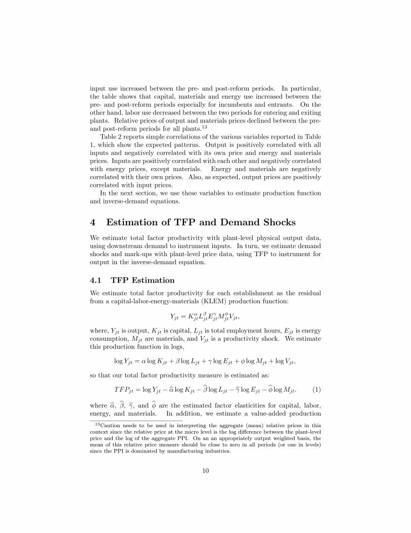
4 Estimation of TFP and Demand Shocks

We estimate total factor productivity with plant-level physical output data,using downstream demand to instrument inputs. In turn, we estimate demandshocks and mark-ups with plant-level price data, using TFP to instrument foroutput in the inverse-demand equation.

4.1 TFP Estimation

We estimate total factor productivity for each establishment as the residualfrom a capital-labor-energy-materials (KLEM) production function:

Yjt = KαjtL

βjtE

γjtM

φjtVjt,

where, Yjt is output, Kjt is capital, Ljt is total employment hours, Ejt is energyconsumption, Mjt are materials, and Vjt is a productivity shock. We estimatethis production function in logs,

log Yjt = α logKjt + β logLjt + γ logEjt + φ logMjt + log Vjt,

so that our total factor productivity measure is estimated as:

TFPjt = log Yjt − bα logKjt − bβ logLjt − bγ logEjt − bφ logMjt. (1)

where bα, bβ, bγ, and bφ are the estimated factor elasticities for capital, labor,energy, and materials. In addition, we estimate a value-added production

13Caution needs to be used in interpreting the aggregate (mean) relative prices in thiscontext since the relative price at the micro level is the log difference between the plant-levelprice and the log of the aggregate PPI. On an an appropriately output weighted basis, themean of this relative price measure should be close to zero in all periods (or one in levels)since the PPI is dominated by manufacturing industries.

10

function with only capital and labor to provide a benchmark of comparison withother studies. Whether we estimate value-added or KLEM specifications, usingOLS to estimate the production function is likely to generate biased estimates offactor elasticities as productivity shocks are likely to be correlated with capital,labor, energy, and materials. For example, the introduction of capital-biasedtechnologies is likely to be associated with greater use of capital and energy andwith less employment.We deal with this omitted variable bias by using demand-shift instruments

which are correlated with input use but uncorrelated with productivity shocks.In particular, we construct Shea (1993) and Syverson (2003) type instruments byselecting industries whose output fluctuations are likely to function as approx-imately exogenous demand shocks for other industries. The instruments aretotal output measures in downstream industries, or combinations of downstreamindustries, that satisfy two conditions: (1) they buy a large enough fraction ofthe output generated by the upstream industry (i.e., the relevance condition),and (2) their purchases from the output industry are a relatively small share oftheir costs (i.e., the exogeneity condition). The latter condition is important toensure that the upstream industry is not affecting the downstream industry, sothat the instrument - downstream demand - is uncorrelated with productivityshocks upstream. The first condition is important to ensure relevance of theinstruments, i.e., strong correlations between the instruments and use of inputsupstream. Following Shea (1993), we use the input-output matrix for everyyear to construct instruments for the equivalent of two-digit industries in theU.S.14 For the instruments to meet the two criteria above, we impose that: (1)the demand share of the downstream industry for upstream production has toexceed 15%, and (2) the cost share of the upstream industry products in thedownstream’s total costs is less than 15 percent.15 We also use the second,third, and fourth degree polynomials as well as one- and two-period lags of thedemand shifters. The rationale for doing this is that some factors, such ascapital and labor, may face non-linear adjustment costs and irreversibilities, so

14We use input-output matrices from the national accounts for the pre-1994 period. For thelater years, a new methodology was put in place for the national accounts, and input-outputmatrices were replaced by output-use and output-supply matrices. For these later years, weuse the output-use matrices to determine cost and sales shares, and the output-supply matricesto determine sectoral output. It is also important to note that input-output matrices do notuse ISIC codes to classify industries. The level at which we could create concordance is closeto the 2-digits ISIC codes.15While Shea(1997) uses a criterion of exogeneity based on the ratio of demand share to

cost share (i.e., this ratio being less than 3), our criterion is based on absolute cost shares(i.e., having a cost share of less than 15%). This absolute criterion is more binding than theratio criterion for downstream industries that represent large demand shares, and less bindingfor other dowsntream industries. Using the above criteria, adding exports to the downstreamdemand set and also aggregrating downstream industries to two or three industries to meetthe greater than 15% threshold, we obtain instruments for 8 of the 12 upstream industries(i.e., Drinks and Beverages, Wood, Food, Textiles, Oil, Paper, Chemicals and Rubber, andGlass and other non-metallic products). The 4 sectors without demand-shift instruments areTobacco, which makes up a very low share of sales for other industries; Metals and Machinery,which comprise too high a share of costs when the sales share is high enough; and OtherManufacturing for which the two criteria are not met.

11

that demand shifts may have non-linear effects and take various periods to affectfactor utilization. In addition, we use regional GDP for the region where theplant is located as an instrument to capture shifts in local demand.16 We re-gard this instrument as particularly relevant to identify the coefficient on labor,given that labor markets in Colombia are largely region-specific. Finally, weuse energy and materials prices as instruments, which are negatively correlatedto energy consumption and use of materials, but likely to be uncorrelated withproductivity shocks.Table 3 reports results for the value-added specification with only capital and

labor and for the KLEM specification of the production function. Column (1)reports the OLS results from the estimation of the value-added specification.The results show an elasticity for capital of about 0.26 and an elasticity forlabor of about 0.81, which are in line with other studies. The problem withthis specification in terms of estimating total factor productivity is, however,that it imposes implausible restrictions in terms of the elasticity of output toenergy and materials. For this reason, we estimate a KLEM specificationwhich uses physical output in the left-hand side and also includes energy andmaterials as inputs. Column (2) presents the OLS results from the estimationof the KLEM specification. As expected, factor elasticities for capital and laborbecome smaller, as energy and materials are being included. The results nowsuggest elasticities for capital, labor, energy, and materials of 0.06, 0.25, 0.13,and 0.6, respectively.However, as pointed out above, these elasticities are likely to be biased if

productivity shocks are correlated with input use. Columns (3) and (4) ofTable 3 present results using 2SLS estimation, which rely on the demand-shiftinstruments, regional GDP, and input prices. Even if we think these instru-ments are weakly correlated with productivity shocks, large biases could beintroduced when using IV estimation if instruments are weakly correlated withthe inputs. To check whether inputs are highly and significantly correlatedwith the instruments, Table 4 reports results for the first-stages of the inputson the various instruments. The results suggest use of capital, energy, and ma-terials increases significantly with downstream demand at an increasing rate,but employment hours decrease significantly with downstream demand at a de-creasing rate. Regional GDP is positively and strongly correlated with laborand materials and negatively correlated with energy consumption, but uncorre-lated with capital. Also, as expected, materials and energy prices significantly

16There may be a common component in technology shocks, although given the enormousheterogeneity across plants the idiosyncratic component dominates. The common componentof technology shocks would be correlated with national GDP (so we do not use national GDP asan instrument) but is less likely to be highly correlated with state/regional GDP fluctuations.In future drafts, we plan to investigate alternative measures of local demand variation. Itis also worth emphasizing that results in the remainder of the paper are robust to exclusionof this instrument. That is, we obtain virtually the same results for the estimation of theproduction functions and all the results that depend upon our TFP estimates. A modest butimportant exception is that when we exclude regional GDP in our instrument list, we findthat entrants are typically not different from incumbents at the point of entry. However, westill find the same learning effects post-reform that we find with the current instrument list.

12

reduce energy consumption and use of materials and capital, but not employ-ment hours. Given that we are considering instrument relevance with multipleendogenous regressors, we report the partial R2 measures suggested by Shea(1997) for the first-stages, which capture the correlation between an endoge-nous regressor and the instruments after taking away the correlation betweenthat particular regressor with all other endogenous regressors.17 The partialR2’s for capital, labor hours, energy, and materials in the KLEM specificationare 0.1718, 0.2213, 0.2876, and 0.4021, respectively, and 0.3235 and 0.2186 forcapital and labor in the value-added specification, showing that the relevantinstruments for each input can explain a substantial fraction of the variation inthe use of that input.The IV results for the value-added specification in Column (3) of Table 3

show a larger capital elasticity and a similar labor elasticity relative to the OLSestimated elasticities. The results in Column (4) of Table 3 show instead smallerelasticities for capital and materials and larger elasticities for labor and energy,when inputs are instrumented.18 The results from the KLEM specification,thus, indicate that productivity shocks during the period of study are positivelycorrelated with capital and materials and negatively correlated with labor andenergy, suggesting the adoption of capital-biased and energy-saving technologiesin Colombia during the 1980’s and 1990’s.

4.2 Estimation of Demand Shocks

While productivity is likely one of the crucial components of profitability in-fluencing market selection, other components of profitability are also probablyimportant determinants of firm entry and exit. For example, even if plants arehighly productive, they may be forced to exit the market if faced with largenegative demand shocks. We capture the demand component of profitabilityby estimating establishment-level demand shocks as the residual of the followinginverse-demand equation:19

Pjt = Y−εjt Djt,

whereDjt is a demand shock faced by firm j at time t and −ε is the inverse of theelasticity of demand and 1+ε is the mark-up. We estimate this inverse-demand

17The standard R2 simply reports the square of the sample correlation coefficient betweenIjt on Ijt, where I = K,L,E,M and Ijt are the predicted values of the inputs from a regres-sion of Ijt on the instruments. The partial R

2 reports the square of the sample correlationcoefficient between gjt and bgjt, where gjt are the residuals from an OLS regression of Ijt on

all other inputs I1jt and bgjt are the residuals from an OLS regression of Ijt on the predicted

values of all other inputs I1jt.18The value-added specification ignores changes in capital utilization. These changes are

likely highly correlated with energy usage, and therefore will be captured by the elasticity ofenergy in the KLEM specification. This fact may explain why the capital elasticity in thevalue-added equation grows when using instruments, while the opposite occurs for the KLEMequation.19There are other important components of profitability that we do not measure, such as

access to credit markets.

13

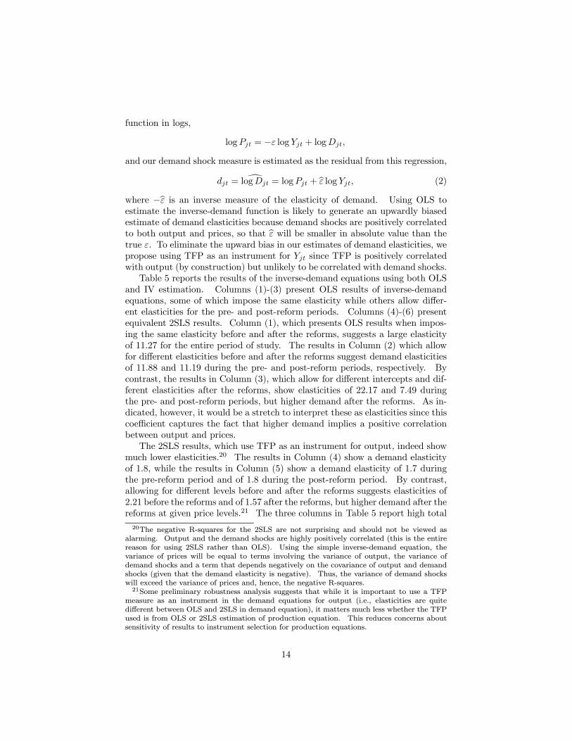
function in logs,

logPjt = −ε log Yjt + logDjt,and our demand shock measure is estimated as the residual from this regression,

djt = dlogDjt = logPjt + bε log Yjt, (2)

where −bε is an inverse measure of the elasticity of demand. Using OLS toestimate the inverse-demand function is likely to generate an upwardly biasedestimate of demand elasticities because demand shocks are positively correlatedto both output and prices, so that bε will be smaller in absolute value than thetrue ε. To eliminate the upward bias in our estimates of demand elasticities, wepropose using TFP as an instrument for Yjt since TFP is positively correlatedwith output (by construction) but unlikely to be correlated with demand shocks.Table 5 reports the results of the inverse-demand equations using both OLS

and IV estimation. Columns (1)-(3) present OLS results of inverse-demandequations, some of which impose the same elasticity while others allow differ-ent elasticities for the pre- and post-reform periods. Columns (4)-(6) presentequivalent 2SLS results. Column (1), which presents OLS results when impos-ing the same elasticity before and after the reforms, suggests a large elasticityof 11.27 for the entire period of study. The results in Column (2) which allowfor different elasticities before and after the reforms suggest demand elasticitiesof 11.88 and 11.19 during the pre- and post-reform periods, respectively. Bycontrast, the results in Column (3), which allow for different intercepts and dif-ferent elasticities after the reforms, show elasticities of 22.17 and 7.49 duringthe pre- and post-reform periods, but higher demand after the reforms. As in-dicated, however, it would be a stretch to interpret these as elasticities since thiscoefficient captures the fact that higher demand implies a positive correlationbetween output and prices.The 2SLS results, which use TFP as an instrument for output, indeed show

much lower elasticities.20 The results in Column (4) show a demand elasticityof 1.8, while the results in Column (5) show a demand elasticity of 1.7 duringthe pre-reform period and of 1.8 during the post-reform period. By contrast,allowing for different levels before and after the reforms suggests elasticities of2.21 before the reforms and of 1.57 after the reforms, but higher demand after thereforms at given price levels.21 The three columns in Table 5 report high total

20The negative R-squares for the 2SLS are not surprising and should not be viewed asalarming. Output and the demand shocks are highly positively correlated (this is the entirereason for using 2SLS rather than OLS). Using the simple inverse-demand equation, thevariance of prices will be equal to terms involving the variance of output, the variance ofdemand shocks and a term that depends negatively on the covariance of output and demandshocks (given that the demand elasticity is negative). Thus, the variance of demand shockswill exceed the variance of prices and, hence, the negative R-squares.21Some preliminary robustness analysis suggests that while it is important to use a TFP

measure as an instrument in the demand equations for output (i.e., elasticities are quitedifferent between OLS and 2SLS in demand equation), it matters much less whether the TFPused is from OLS or 2SLS estimation of production equation. This reduces concerns aboutsensitivity of results to instrument selection for production equations.

14

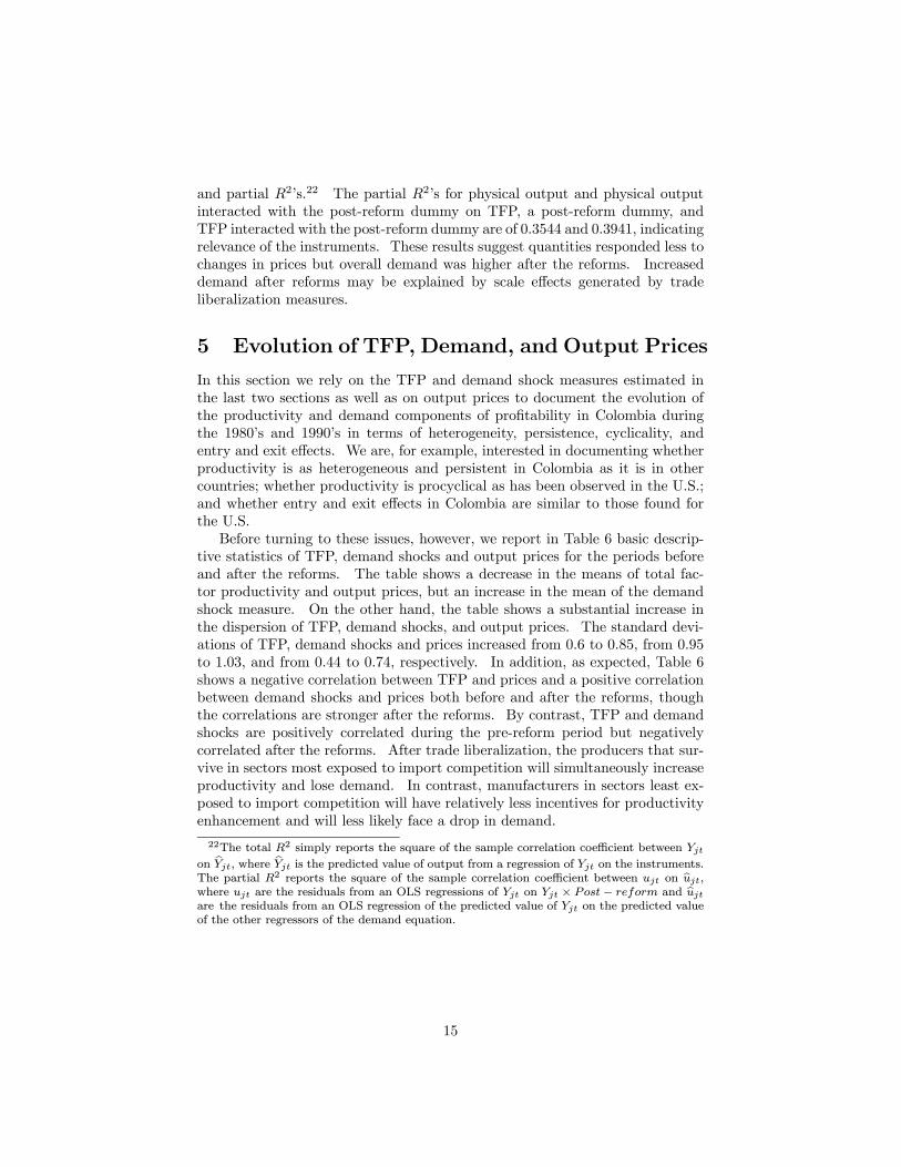
and partial R2’s.22 The partial R2’s for physical output and physical outputinteracted with the post-reform dummy on TFP, a post-reform dummy, andTFP interacted with the post-reform dummy are of 0.3544 and 0.3941, indicatingrelevance of the instruments. These results suggest quantities responded less tochanges in prices but overall demand was higher after the reforms. Increaseddemand after reforms may be explained by scale effects generated by tradeliberalization measures.

5 Evolution of TFP, Demand, and Output Prices

In this section we rely on the TFP and demand shock measures estimated inthe last two sections as well as on output prices to document the evolution ofthe productivity and demand components of profitability in Colombia duringthe 1980’s and 1990’s in terms of heterogeneity, persistence, cyclicality, andentry and exit effects. We are, for example, interested in documenting whetherproductivity is as heterogeneous and persistent in Colombia as it is in othercountries; whether productivity is procyclical as has been observed in the U.S.;and whether entry and exit effects in Colombia are similar to those found forthe U.S.Before turning to these issues, however, we report in Table 6 basic descrip-

tive statistics of TFP, demand shocks and output prices for the periods beforeand after the reforms. The table shows a decrease in the means of total fac-tor productivity and output prices, but an increase in the mean of the demandshock measure. On the other hand, the table shows a substantial increase inthe dispersion of TFP, demand shocks, and output prices. The standard devi-ations of TFP, demand shocks and prices increased from 0.6 to 0.85, from 0.95to 1.03, and from 0.44 to 0.74, respectively. In addition, as expected, Table 6shows a negative correlation between TFP and prices and a positive correlationbetween demand shocks and prices both before and after the reforms, thoughthe correlations are stronger after the reforms. By contrast, TFP and demandshocks are positively correlated during the pre-reform period but negativelycorrelated after the reforms. After trade liberalization, the producers that sur-vive in sectors most exposed to import competition will simultaneously increaseproductivity and lose demand. In contrast, manufacturers in sectors least ex-posed to import competition will have relatively less incentives for productivityenhancement and will less likely face a drop in demand.

22The total R2 simply reports the square of the sample correlation coefficient between Yjton bYjt, where bYjt is the predicted value of output from a regression of Yjt on the instruments.The partial R2 reports the square of the sample correlation coefficient between ujt on bujt,where ujt are the residuals from an OLS regressions of Yjt on Yjt × Post− reform and bujtare the residuals from an OLS regression of the predicted value of Yjt on the predicted valueof the other regressors of the demand equation.

15

5.1 Heterogeneity

Previous evidence for the US suggests a pattern of evolving common produc-tivity and prices among heterogeneous plants (Baily, Hulten and Campbell(1992); Foster, Haltiwanger and Krizan (2002); Foster, Haltiwanger and Syver-son (2003); Supina and Roberts (1996)). Like in the U.S., dispersion measuresin Table 6 suggest much heterogeneity in productivity and prices across Colom-bian plants. Figures 1-3 show the evolution of dispersion measures of TFP,demand shocks and output prices for continuing, entering, and exiting plantsover the period of study. The figures show large percentage increases in thedispersion of productivity and prices over the last two decades. In particular,Figures 1 and 3 show large rises in the dispersion of productivity and prices of en-tering and exiting plants after 1990. By contrast, Figure 2 shows a much smallerpercentage increase in the dispersion of demand over the last two decades. Thegreater heterogeneity in productivity is consistent with greater process exper-imentation across businesses after reforms, while the modest increase in thedispersion of demand is consistent with modest increased experimentation inproduct variety across businesses.23

5.2 Persistence

To examine whether Colombian plants, like U.S. plants, are characterized by alarge degree of persistence, we estimate AR(1) models for productivity, demandshocks and prices. Columns (1), (3) and (5) in Table 7 report the coefficients onthe lags of productivity, demand and output prices for AR(1) models with yeareffects. The results show a great deal of persistence of productivity, demandshocks and prices in Colombia and much greater than for the U.S. The resultssuggest that 65% of all plants continue with their initial productivity after 5years, 93% of plants face the same demand shocks after 5 years, and 96% chargethe same prices as 5 years ago. Studies for the U.S. find much lower degreesof persistence. For example, Bartelsman and Dhrymes (1998) find that after 5years only about a third of all plants remain in the same productivity quintile.Foster, Haltiwanger and Syverson (2003) also find that about a third of plantsremain in their original position in the productivity and price distributionsafter 5 years. The greater persistence in the Colombian context probablyreflects continued lack of competition in the Colombian economy, in spite of thereforms. This may be due to the partial nature of a short-lived reform processthat was not followed through to eliminate remaining frictions, as was the casein other reformist nations.

23Two related measurement points are worth noting in this context. First, we found thatdispersion in TFP increased dramatically in 1996 for what we perceive to be spurious reasons.For the plots of TFP dispersion we have simply interpolated the 1996 values. Second, we haveexamined these patterns using alternative robust measures of dispersion (in particular, the90-10 differential) and have found very similar patterns overall for TFP, prices and demandshocks. Interestingly, we also found a seemingly spurious increase in dispersion in 1996 usingthese more robust measures of dispersion suggesting the measurement problems for dispersionof TFP in 1996 are not being driven by outliers.

16

Columns (2), (4), and (6) in Table 7 also reports how the persistence changesafter the market reforms. The results suggest persistence increased only slightly.At first glance, this pattern might be surprising as one might conjecture thatmarket reforms would lead to greater mobility and flexibility in the efficiencydistribution and demand distributions. However, it is important to emphasizethat these persistence measures are conditional on survival. As documentedbelow, survival becomes increasingly a function of market fundamentals after re-forms, suggesting plants are adjusting at the external margin rather the internalmargin. That is, plant survival responds more after the reforms, but survivingplants are less likely to move up or down in the distribution after reforms.

5.3 Cyclicality

While there is quite a lot of persistence in productivity and demand shocks,productivity and demand shocks also tend to move over the business cycle.Previous papers for the U.S., including papers by Hall (1990), Bartelsman,Caballero and Lyons (1994), and Basu and Fernald (1997), document and tryto explain the procyclicality of productivity in the U.S. Baily, Bartelsmanand Haltiwanger (2001) show that the procyclicality at the aggregate level ismimicked at the micro level. Overall, however, the procyclical productivitypuzzle remains unresolved. Here, we examine whether such procyclicality isalso observed in the Colombian context.Figures 4-6 show productivity, demand shock and price movements for con-

tinuing, entering and exiting firms from 1982-1999, where the figures includeGDP growth on the right-hand side axis to be able to understand movementswith the cycle. Colombia experienced three recessions and two booms duringthe period of study. The first recession took place during the early 1980’s,the second during the period from 1988 to 1991, and the third and strongestrecession since the Great Depression after 1995 and until the present. The twobooms took place from 1985 to 1988 and from 1991 to 1995.Figure 4 shows a highly volatile productivity growth for the average plant

and even more for the average entering and exiting plant. Volatility has in-creased over time and, interestingly, the pattern of average productivity at theplant level changes from being countercyclical prior to reforms to being procyli-cal after the reforms. For example, the correlation of average plant productivitywith GDP growth for continuing plants is -0.43 pre-reform and 0.39 post-reform.Interestingly, the productivity of entering and exiting plants becomes much morecyclical also after reforms. After reforms, productivity for entrants becomesstrongly countercyclical, while the productivity for exiting businesses becomesmildly procyclical. Both of these patterns deserve more investigation, but atleast some aspects of these results make sense from a market selection perspec-tive. After reforms, in good times there might be more experimentation byentrants so the average entrant is less productive (upon entry at least). Theresult also suggest that, after reforms, the threshold for exiting increases in goodtimes.Figure 5 and Figure 6 show the patterns of the average demand shocks and

17

average relative price for all, continuing, entering and exiting plants. Almostby construction average relative prices exhibit little movement.24 Figure 5shows that the average demand shocks are more volatile, especially after marketreforms when they become procyclical. Caution should be used in interpretingthese average demand shocks since these reflect the average of the demandshocks from a micro model of relative prices across plants. Thus, these are notaggregate demand or even manufacturing demand (say relative to other sectors)shocks as the relative price for the plant is the price of the output for the plantrelative to the PPI (which is essentially the weighted average price across allmanufacturing plants).

5.4 Entry and Exit Effects

Vintage capital models of industry dynamics suggest new firms receive the pro-ductivity associated with the latest vintage technology, and productivity re-mains constant over time unless hit by random shocks. Then, firms exit themarket when the productivity relative to new entrants is below a certain thresh-old. However, aside from Foster, Haltiwanger and Syverson (2003) who findhigher productivity of entering plants and lower productivity of exiting plants,the previous literature documents lower productivity of both entering and ex-iting relative to incumbent plants (see Bartelsman and Doms (2000)), which isat odds with the vintage capital model.Table 8 reports regressions of TFP, demand shocks, and prices on year dum-

mies as well as on entry and exit dummies. Column (1) in Table 8 showsthat productivity of entering plants is above and productivity of exiting plantsbelow that of the average incumbent. Our results coincide with those in Fos-ter, Haltiwanger, and Syverson (2003). Like theirs, our TFP estimation usesphysical output rather than revenue, which avoids confounding price and pro-ductivity variations in measures of TFP. The results in Column (5) also showlower idiosyncratic demand for entering and exiting plants relative to the aver-age incumbent, but the results in Column (9) show entrants and exiting plantscharging higher prices than incumbents. While the higher prices of exitingplants is consistent with their lower productivity, the higher prices of enteringplants might reflect their smaller scale or perhaps higher markups.Since the reforms introduced during the 1990’s are generally expected to

increase competition, we also explore whether the productivity, demand andprices of entering and exiting plants relative to incumbents changed after theimplementation of these reforms by interacting the entry and exit dummies witha post-reform dummy which takes the value of 1 for the period 1990-1999. Theresults in Column (2) of Table 8 show no differential entry effect on productivityafter the reforms. That is, after the reforms, entering businesses no longer hadany productivity advantage relative to incumbents in the year of entry. Onthe other hand, the results suggest that productivity of exiting plants relative

24The relative prices do become significantly procyclical after reforms, but the magnitudeof the variation is quite small.

18

to incumbents fell substantially after the reforms. Lower adjustment costs dueto less distorted factor markets appear to show a greater reaction of survivingincumbents to entry. First, they can retool more frequently to install latestvintage technologies. Second, this is consistent with increased mass layoffsof unproductive workers after the reduction in dismissal costs in 1990. Thispattern is also consistent with increased exit of plants which may had beenkept afloat by subsidized credit, relatively low taxes, and lack of internationalcompetition before 1990. On net, the contribution of entry and exit risesslightly. Moreover, the results show that relative demand for entering andexiting plants did not change after the reforms. On the other hand, relativeprices of both entering and exiting plants increased after the reforms.We also examine learning effects by looking at the evolution of productivity,

demand, and prices of plants the longer they have been in the market. Theresults in Column (3) of Table 8 for the entire period, which includes one-and two-period lags of the entry dummies and one- and two-period leads ofexit dummies, show no evidence of learning, but they do show evidence thatthe shadow of death effect becomes stronger the closer to exiting the plant is.Interestingly, allowing for differential effects before and after the reforms doesshow some evidence of learning effects after the reforms were introduced, thoughthe coefficients are estimated imprecisely. Learning is more evident in terms ofdemand and prices. In particular, Column (7) and (11) show that the longersince plant entry, the higher relative demand and the lower the prices chargedfor the output. Similarly, these results show that the closer to exiting themarket, the lower relative demand and the higher relative prices. Columns (8)and (12) show greater demand increases and price drops the longer entrantshave been in the market, after the reforms. Moreover, the results show greaterreductions in demand and greater increases in prices the closer the plant is fromexiting, after the reforms.The results suggest that market reforms yielded a more heterogenous group

of entrants, but that conditional on survival the post-reform entrants contributemore to productivity growth. Subsidized credit prior to the 1990 and 1991financial reforms may have previously encouraged entry of unproductive plantsand kept existing unproductive plants afloat. In addition, lower tariffs as aresult of trade liberalization may have increased market discipline by forcingfirms either to increase productivity and charge lower prices or else exit themarket. Moreover, the greater learning after reforms may be due to greateraccess to new vintages of imported capital and greater access to the know-howof foreign firms in the economy.

6 Effects of Efficiency and Demand on Survival

According to selection models of industry dynamics (e.g., Jovanovic (1982),Hopenhayn (1992), Ericson and Pakes (1995), and Melitz (2003)), producersshould continue operations if the discounted value of future profits exceeds theopportunity cost of remaining in operation. In these models, thus, plants’ exit

19

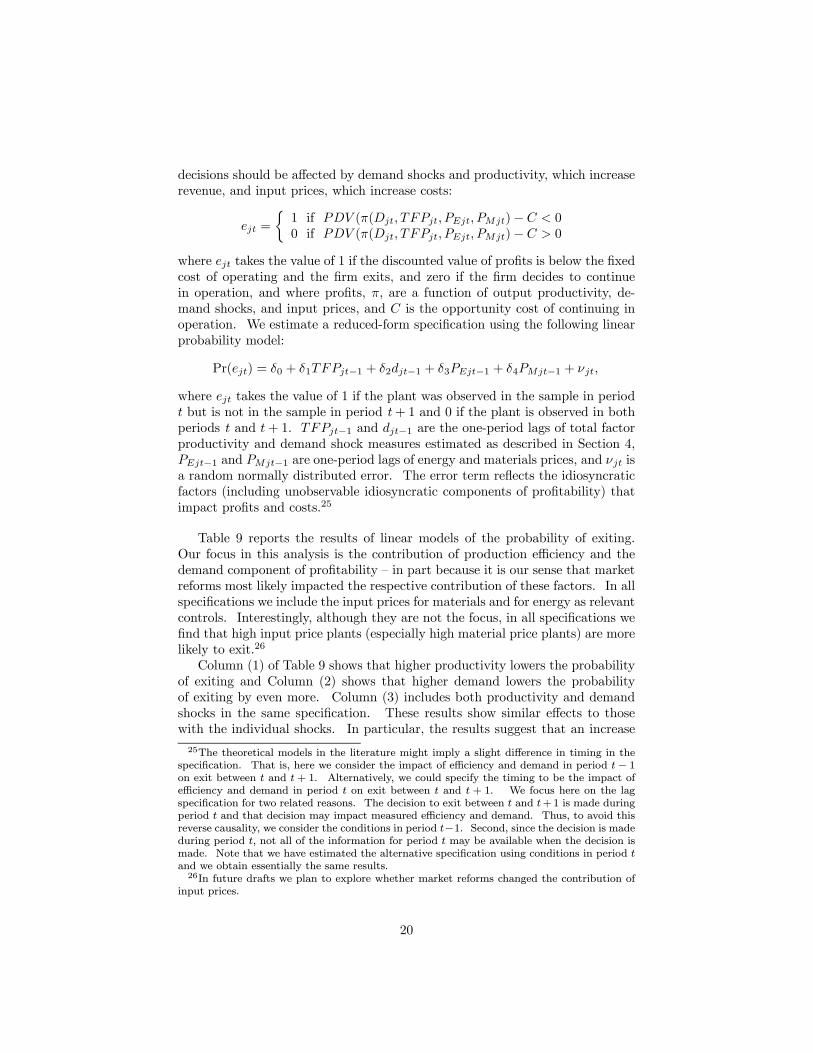
decisions should be affected by demand shocks and productivity, which increaserevenue, and input prices, which increase costs:

ejt =

½1 if PDV (π(Djt, TFPjt, PEjt, PMjt)− C < 00 if PDV (π(Djt, TFPjt, PEjt, PMjt)− C > 0

where ejt takes the value of 1 if the discounted value of profits is below the fixedcost of operating and the firm exits, and zero if the firm decides to continuein operation, and where profits, π, are a function of output productivity, de-mand shocks, and input prices, and C is the opportunity cost of continuing inoperation. We estimate a reduced-form specification using the following linearprobability model:

Pr(ejt) = δ0 + δ1TFPjt−1 + δ2djt−1 + δ3PEjt−1 + δ4PMjt−1 + νjt,

where ejt takes the value of 1 if the plant was observed in the sample in periodt but is not in the sample in period t+ 1 and 0 if the plant is observed in bothperiods t and t+ 1. TFPjt−1 and djt−1 are the one-period lags of total factorproductivity and demand shock measures estimated as described in Section 4,PEjt−1 and PMjt−1 are one-period lags of energy and materials prices, and νjt isa random normally distributed error. The error term reflects the idiosyncraticfactors (including unobservable idiosyncratic components of profitability) thatimpact profits and costs.25

Table 9 reports the results of linear models of the probability of exiting.Our focus in this analysis is the contribution of production efficiency and thedemand component of profitability — in part because it is our sense that marketreforms most likely impacted the respective contribution of these factors. In allspecifications we include the input prices for materials and for energy as relevantcontrols. Interestingly, although they are not the focus, in all specifications wefind that high input price plants (especially high material price plants) are morelikely to exit.26

Column (1) of Table 9 shows that higher productivity lowers the probabilityof exiting and Column (2) shows that higher demand lowers the probabilityof exiting by even more. Column (3) includes both productivity and demandshocks in the same specification. These results show similar effects to thosewith the individual shocks. In particular, the results suggest that an increase

25The theoretical models in the literature might imply a slight difference in timing in thespecification. That is, here we consider the impact of efficiency and demand in period t− 1on exit between t and t + 1. Alternatively, we could specify the timing to be the impact ofefficiency and demand in period t on exit between t and t + 1. We focus here on the lagspecification for two related reasons. The decision to exit between t and t+1 is made duringperiod t and that decision may impact measured efficiency and demand. Thus, to avoid thisreverse causality, we consider the conditions in period t−1. Second, since the decision is madeduring period t, not all of the information for period t may be available when the decision ismade. Note that we have estimated the alternative specification using conditions in period tand we obtain essentially the same results.26In future drafts we plan to explore whether market reforms changed the contribution of

input prices.

20

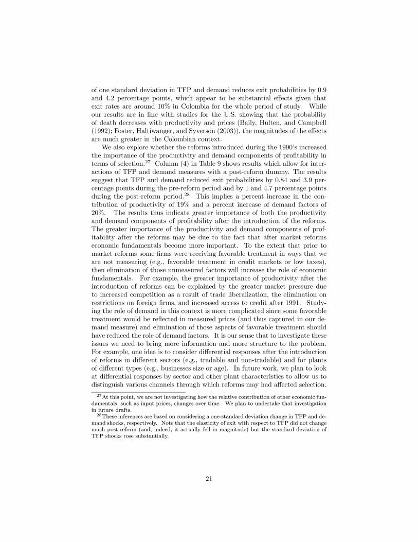
of one standard deviation in TFP and demand reduces exit probabilities by 0.9and 4.2 percentage points, which appear to be substantial effects given thatexit rates are around 10% in Colombia for the whole period of study. Whileour results are in line with studies for the U.S. showing that the probabilityof death decreases with productivity and prices (Baily, Hulten, and Campbell(1992); Foster, Haltiwanger, and Syverson (2003)), the magnitudes of the effectsare much greater in the Colombian context.We also explore whether the reforms introduced during the 1990’s increased

the importance of the productivity and demand components of profitability interms of selection.27 Column (4) in Table 9 shows results which allow for inter-actions of TFP and demand measures with a post-reform dummy. The resultssuggest that TFP and demand reduced exit probabilities by 0.84 and 3.9 per-centage points during the pre-reform period and by 1 and 4.7 percentage pointsduring the post-reform period.28 This implies a percent increase in the con-tribution of productivity of 19% and a percent increase of demand factors of20%. The results thus indicate greater importance of both the productivityand demand components of profitability after the introduction of the reforms.The greater importance of the productivity and demand components of prof-itability after the reforms may be due to the fact that after market reformseconomic fundamentals become more important. To the extent that prior tomarket reforms some firms were receiving favorable treatment in ways that weare not measuring (e.g., favorable treatment in credit markets or low taxes),then elimination of those unmeasured factors will increase the role of economicfundamentals. For example, the greater importance of productivity after theintroduction of reforms can be explained by the greater market pressure dueto increased competition as a result of trade liberalization, the elimination onrestrictions on foreign firms, and increased access to credit after 1991. Study-ing the role of demand in this context is more complicated since some favorabletreatment would be reflected in measured prices (and thus captured in our de-mand measure) and elimination of those aspects of favorable treatment shouldhave reduced the role of demand factors. It is our sense that to investigate theseissues we need to bring more information and more structure to the problem.For example, one idea is to consider differential responses after the introductionof reforms in different sectors (e.g., tradable and non-tradable) and for plantsof different types (e.g., businesses size or age). In future work, we plan to lookat differential responses by sector and other plant characteristics to allow us todistinguish various channels through which reforms may had affected selection.

27At this point, we are not investigating how the relative contribution of other economic fun-damentals, such as input prices, changes over time. We plan to undertake that investigationin future drafts.28These inferences are based on considering a one-standard deviation change in TFP and de-

mand shocks, respectively. Note that the elasticity of exit with respect to TFP did not changemuch post-reform (and, indeed, it actually fell in magnitude) but the standard deviation ofTFP shocks rose substantially.

21

7 Conclusion

In this paper, we examine how reallocation contributes to productivity andprofitability in Colombia, and we then ask how the relation between reallocationand productivity and profitability changed after market reforms were introducedin Colombia during the early 1990’s. The extent, breadth and swiftness of thereforms make Colombia a superb country to study these issues. In addition, aunique feature of the Colombian data is that it allows us to measure both plant-level quantities and prices, making these data ideal for measuring plant-levelproductivity and demand.We generate measures of plant-level total factor productivity by estimating

KLEM production functions using plant-level physical output data. To elim-inate biases from the correlation between productivity shocks and inputs, weuse downstream demand shifts and plant-level energy and materials prices asinstruments in estimating production functions. We then generate plant-leveldemand shocks by estimating inverse-demand equations using plant-level out-put prices, where output is instrumented with TFP to eliminate biases from thecorrelation between demand shocks and output.We find some interesting patterns with regards to total factor productiv-

ity, prices and demand shocks in Colombia, which sometimes contrast withthe patterns found for the U.S. First, as in the U.S., we find a great deal ofheterogeneity in terms of productivity and output prices, and we find that thisheterogeneity has been increasing over the past decades. Second, we find a greatdeal of persistence in productivity, prices and demand, which doubles or triplesthe degree of persistence in the U.S. Third, we find countercyclical movementsin productivity before the reforms, which contrasts with the procyclicality ofproductivity found in the U.S, but procyclical movements in productivity afterthe reforms. The greater persistence in the Colombian context and the changein the cyclicality of productivity after the reforms deserve further investigation.More importantly, we focus on market selection dynamics in Colombia dur-

ing the entire period of study as well as before and after the introduction of re-forms. Consistent with vintage capital models and with recent evidence for theU.S. using plant-level prices, we find that entering business are more productivethan incumbents and the exiting businesses they are replacing, and that exit-ing businesses are less productive than incumbents. Note that revenue-basedTFP measures spuriously include a demand component and thus underestimatetechnical efficiency of entrants, who have to build a consumer base, relative toincumbents, who have a established clientele. Hence, the analysis in the presentpaper provides a better basis to discern between vintage and learning explana-tions for dynamics and heterogeneity in productivity. In addition, we find thatmarket selection is affected by demand-side factors, as both entering and ex-iting plants face lower demand for their products than incumbents. Finally,consistent with these patterns, we find that the probability of death decreaseswith productivity and demand for the products of the business.In addition, we explore how these patterns changed in response to market

reforms. After the reforms, entering businesses no longer had any productivity

22

advantage relative to incumbents, but the productivity of exiting plants relativeto incumbents falls substantially. On net, the contribution of entry and exitrises slightly. This is consistent with increased mass layoffs of unproductiveworkers, who were previously retained by plants due to high dismissal costs.The pattern is also consistent with increased exit of plants which may had beenkept afloat by subsidized credit, relatively low taxes, and lack of internationalcompetition before 1990. When we explore a more dynamic specification, wefind evidence of learning effects for surviving entrants after the reforms. Tradeliberalization may have well contributed to increased learning. Internationalcompetition may have imposed market discipline, forcing plants to either in-crease productivity and charge lower prices or exit the market. On the otherhand, access to new vintages of imported capital may also well be contributingto productivity growth, especially if lower capital adjustment costs increase theoptimal frequency of retooling to install equipment embedding latest technology.Finally, consistent with these patterns, we find that economic fundamentals (i.e.,efficiency and demand) play a larger role in determining survival after marketreforms. To the extent that prior to market reforms some firms were receivingfavorable treatment, then elimination of these unmeasured factors will increasethe role of economic fundamentals.Our paper takes a first look at the impact of the reforms on the relation

between efficiency and demand-side factors on market selection, by essentiallyasking whether the covariance structure of productivity, demand shocks and netentry changes after the reforms. While instructive, there remains much researchthat should be done in this context and, in particular, to investigate the reformswith more information and structure. In future work, we plan to explore thetemporal and cross-sectional variation of the various reforms more fully. Not allthe market reforms happened at the same time; not all of the market reformswork in the same direction, and many of the market reforms likely impactedfirms differentially depending upon sector and other characteristics (e.g., factorintensities, size, and location) of the businesses.

References

[1] Aghion, Philippe and Howitt. 1992. “ A Model of Growth Through CreativeDestruction,” Econometrica, 60(2): 323-351.

[2] Aw, Bee-Yan, Siaomin Chen, and Mark Roberts. 1997. “Firm-level Evi-dence on Productivity Differentials, Turnover and Exports in TaiwaneseManufacturing, NBER Working Paper 6235.

[3] Bartelsman, Eric, Martin Baily and John Haltiwanger. 2001. “Labor Pro-ductivity: Structural Change and cyclical Dynamics,” Review of Economicsand Statistics, 83(3): 420-433.

23

[4] Bartelsman, Eric and Mark Doms. 2000. “Understanding Productivity:Lessons from Longitudinal Microdata,” Journal of Economic Literature,38(2): 569-594.

[5] Bartelsman, Eric and Phebus Dhrymes. 1998. “Productivity Dynamics:U.S. Manufacturing Plants 1972-1986,” Journal of Productivity Analysis,9(1): 5-34.

[6] Bartelsman, Eric, Ricardo Caballero and Richard Lyons. 1994. “Customer-and Supplier-Driven Externalities,” American Economic Review, 84(4):1075-1084.

[7] Baily, Martin, Charles Hulten and David Campbell. 1992. “ProductivityDynamics in Manufacturing Establishments,” Brookings Papers on Eco-nomic Activity: Microeconomics, 187-249.

[8] Bigsten, Arne, Paul Collier, Stefan Dercon, Bernard Gauthier, Jan GunningAnders Isaksson, Abena Oduro, Remco Oostendrop, Cathy Pattillo, MansSoderbom, Michel Sylvain, Francis Teal and Albert Seufack. 1997. “Exportsand Firm-level Efficiency in the African Manufacturing Sector,” Universityof Montreal.

[9] Basu, Susanto and John Fernald. 1997. “Returns to Scale in U.S. Produc-tion: Estimates and Implications,” Journal of Political Economy, 105(2):249-283.

[10] Burki, Shajid and Guillermo Perry. 1997. The Long March: A ReformAgenda for Latin America and the Caribbean for the Next Decade. Wash-ington D.C.: World Bank.

[11] Chen, Tain-jy and De-piao Tang. 1987. “Comparing Technical EfficiencyBetween Import-Substitution-Oriented and Export-Oriented Foreign Firmsin a Developing Country,” Journal of Development Economics, 36: 277-289.

[12] Davis, Steven, John Haltiwanger and Scott Schuh. 1996. Job Creation andDestruction. Cambridge, Mass.: MIT Press.

[13] Edwards, Sebastian. 2001. The Economic and Political Transition to anOpen Market Economy: Colombia. Paris: OECD.

[14] Ericson, Richard and Ariel Pakes.1995. “Markov-Perfect Industry Dynam-ics: A Framework for Empirical Work,” Review of Economic Studies, 62(1):53-82.

[15] Foster, Lucia, John Haltiwanger, and Chad Syverson. 2003. “Reallocation,Firm Turnover, and Efficiency: Selection on Productivity or Profitability?,”University of Maryland, Mimeo.

24

[16] Foster, Lucia, John Haltiwanger, and Cornell Krizan. 2001. “AggregateProductivity Growth: Lessons from Microeconomic Evidence,” in EdwardDean Michael Harper and Charles Hulten, eds., New Developments in Pro-ductivity Analysis. Chicago: University of Chicago Press.

[17] Hall, Robert. 1990. “Invariance Properties of Solow’s Productivity Resid-ual,” in Peter Diamond, ed., Growth/Productivity/Unemployment. Cam-bridge: MIT Press.

[18] Haltiwanger, John. 2000. “Aggregate Growth: What Have We Learnedfrom Microeconomic Evidence?,” University of Maryland, Mimeo.

[19] Harrison, Ann. 1994. “Productivity, Imperfect Competition, and Trade Re-form: Theory and Evidence,” Journal of International Economics, 36: 53-73.

[20] Hopenhayn, Hugo. 1992. “Entry, Exit, and Firm Dynamics in Long RunEquilibrium,” Econometrica, 60(5): 1127-50.

[21] Jovanovic, Boyan. 1982. “Selection and the Evolution of Industry,” Econo-metrica, 50(3): 649-670.

[22] Kugler, Adriana and Maurice Kugler. 2003. “The Labor Market Effectsof Payroll Taxes in a Middle-Income Country: Evidence from Colombia,”CEPR Working Paper No. 4046.

[23] Kugler, Adriana. 2002. “From Severance Pay to Self-Insurance: The Effectsof Severance Payments Savings Accounts in Colombia,” CEPR WorkingPaper No. 3197.

[24] Kugler, Adriana. 1999. “The Impact of Firing Costs on Turnover and Un-employment: Evidence from the Colombian Labor Market Reform,” Inter-national Tax and Public Finance Journal, 6(3): 389-410.

[25] Kugler, Maurice. 2000. “The Diffusion of Externalities from Foreign DirectInvestment: The Sectoral Pattern of Spillovers,” Essays on InternationalTechnology Diffusion, Chapter 1, Ph.D. Dissertation, UC Berkeley.

[26] Kugler, Maurice and Howard Rosenthal. 2003. “Checks and Balances: AnAssessment of the Institutional Separation of Powers in Colombia,” in Al-berto Alesina, ed., Institutional Reforms in Colombia, MIT Press.

[27] Levinshohn, James and Amil Petrin. 1997. “Productivity, Industry Dynam-ics, and International Competition: A Structural Econometric Approach,”University of Michigan, Mimeo.

[28] Liu, Lili. 1996. “Entry-Exit, Learning and Productivity Change: Evidencefrom Chile,” Journal of Development Economics, 42: 217-42.

25

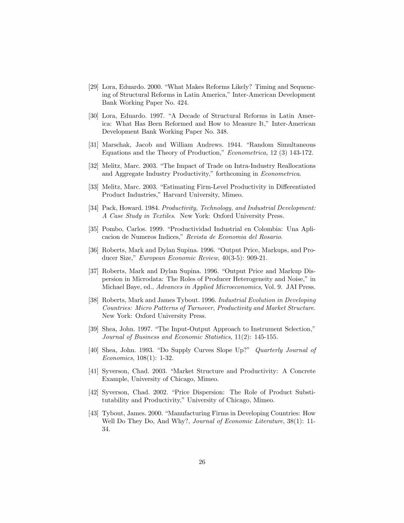
[29] Lora, Eduardo. 2000. “What Makes Reforms Likely? Timing and Sequenc-ing of Structural Reforms in Latin America,” Inter-American DevelopmentBank Working Paper No. 424.

[30] Lora, Eduardo. 1997. “A Decade of Structural Reforms in Latin Amer-ica: What Has Been Reformed and How to Measure It,” Inter-AmericanDevelopment Bank Working Paper No. 348.

[31] Marschak, Jacob and William Andrews. 1944. “Random SimultaneousEquations and the Theory of Production,” Econometrica, 12 (3) 143-172.

[32] Melitz, Marc. 2003. “The Impact of Trade on Intra-Industry Reallocationsand Aggregate Industry Productivity,” forthcoming in Econometrica.

[33] Melitz, Marc. 2003. “Estimating Firm-Level Productivity in DifferentiatedProduct Industries,” Harvard University, Mimeo.

[34] Pack, Howard. 1984. Productivity, Technology, and Industrial Development:A Case Study in Textiles. New York: Oxford University Press.

[35] Pombo, Carlos. 1999. “Productividad Industrial en Colombia: Una Apli-cacion de Numeros Indices,” Revista de Economia del Rosario.

[36] Roberts, Mark and Dylan Supina. 1996. “Output Price, Markups, and Pro-ducer Size,” European Economic Review, 40(3-5): 909-21.

[37] Roberts, Mark and Dylan Supina. 1996. “Output Price and Markup Dis-persion in Microdata: The Roles of Producer Heterogeneity and Noise,” inMichael Baye, ed., Advances in Applied Microeconomics, Vol. 9. JAI Press.

[38] Roberts, Mark and James Tybout. 1996. Industrial Evolution in DevelopingCountries: Micro Patterns of Turnover, Productivity and Market Structure.New York: Oxford University Press.

[39] Shea, John. 1997. “The Input-Output Approach to Instrument Selection,”Journal of Business and Economic Statistics, 11(2): 145-155.

[40] Shea, John. 1993. “Do Supply Curves Slope Up?” Quarterly Journal ofEconomics, 108(1): 1-32.

[41] Syverson, Chad. 2003. “Market Structure and Productivity: A ConcreteExample, University of Chicago, Mimeo.

[42] Syverson, Chad. 2002. “Price Dispersion: The Role of Product Substi-tutability and Productivity,” University of Chicago, Mimeo.

[43] Tybout, James. 2000. “Manufacturing Firms in Developing Countries: HowWell Do They Do, And Why?, Journal of Economic Literature, 38(1): 11-34.

26

[44] Tybout, James and Daniel Westbrook. 1995. “Trade Liberalization andDimensions of Efficiency Change in Mexican Manufacturing Industries,”Journal of International Economics, 39(1-2): 53-78.

27

Figure 1: TFP Dispersion for Continuing, Entering, and Exiting Plants, 1982-1998

0

0.2

0.4

0.6

0.8

1

1.2

1.4

1.6

1.8

1982 1983 1984 1985 1986 1987 1988 1989 1990 1991 1992 1993 1994 1995 1996 1997 1998

TFP

(Sta

ndar

d D

evia

tion)

EXITING ENTERING CONTINUING ALL

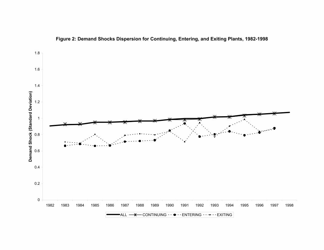
Figure 2: Demand Shocks Dispersion for Continuing, Entering, and Exiting Plants, 1982-1998

0

0.2

0.4

0.6

0.8

1

1.2

1.4

1.6

1.8

1982 1983 1984 1985 1986 1987 1988 1989 1990 1991 1992 1993 1994 1995 1996 1997 1998

Dem

and

Shoc

k (S

tand

ard

Dev

iatio

n)

ALL CONTINUING ENTERING EXITING

Figure 3: Output Prices Dispersion for Continuing, Entering, and Exiting Plants, 1982-1998

0

0.2

0.4

0.6

0.8

1

1.2

1.4

1.6

1.8

1982 1983 1984 1985 1986 1987 1988 1989 1990 1991 1992 1993 1994 1995 1996 1997 1998

Rel

ativ

e pr

ices

(sta

ndar

d de

viat

ion)

ALL CONTINUING ENTERING EXITING

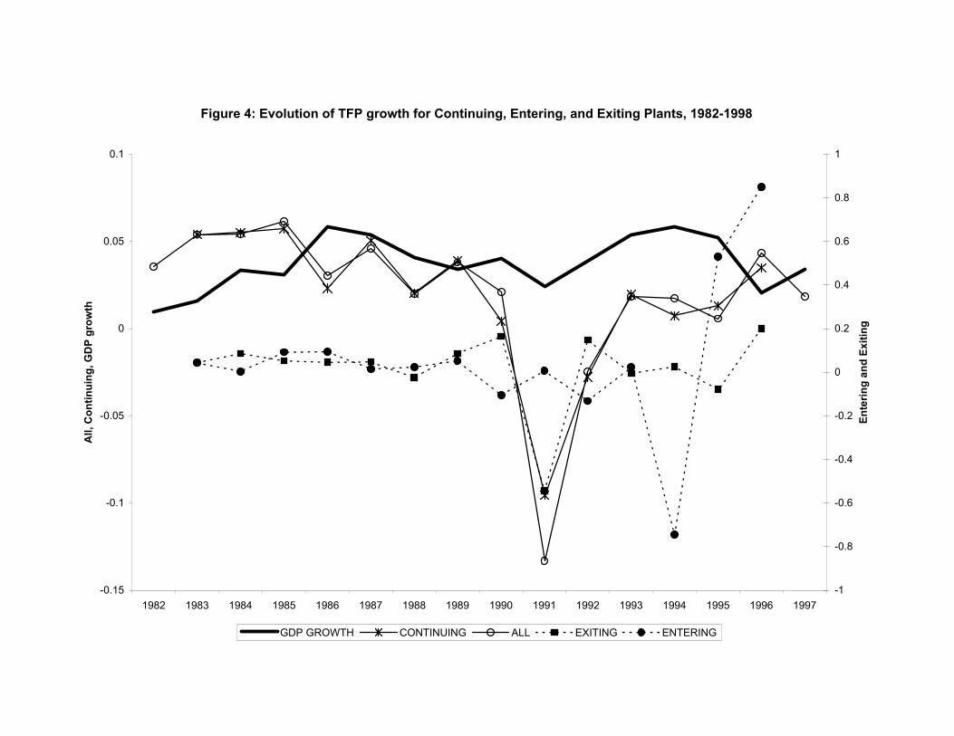
Figure 4: Evolution of TFP growth for Continuing, Entering, and Exiting Plants, 1982-1998

-0.15

-0.1

-0.05

0

0.05

0.1

1982 1983 1984 1985 1986 1987 1988 1989 1990 1991 1992 1993 1994 1995 1996 1997

All,

Con

tinui

ng, G

DP

grow

th

-1

-0.8

-0.6

-0.4

-0.2

0

0.2

0.4

0.6

0.8

1

Ente

ring

and

Exiti

ng

GDP GROWTH CONTINUING ALL EXITING ENTERING

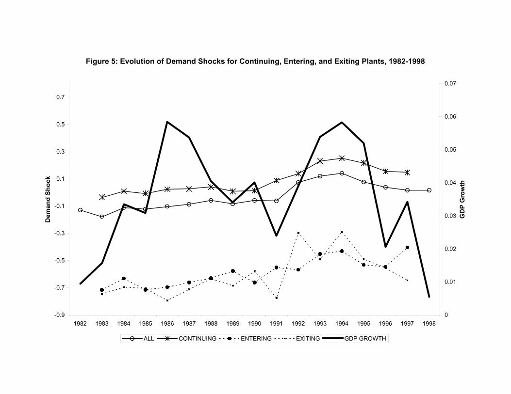
Figure 5: Evolution of Demand Shocks for Continuing, Entering, and Exiting Plants, 1982-1998

-0.9

-0.7

-0.5

-0.3

-0.1

0.1

0.3

0.5

0.7

1982 1983 1984 1985 1986 1987 1988 1989 1990 1991 1992 1993 1994 1995 1996 1997 1998

Dem

and

Shoc

k

0

0.01

0.02

0.03

0.04

0.05

0.06

0.07

GD

P G

row

th

ALL CONTINUING ENTERING EXITING GDP GROWTH

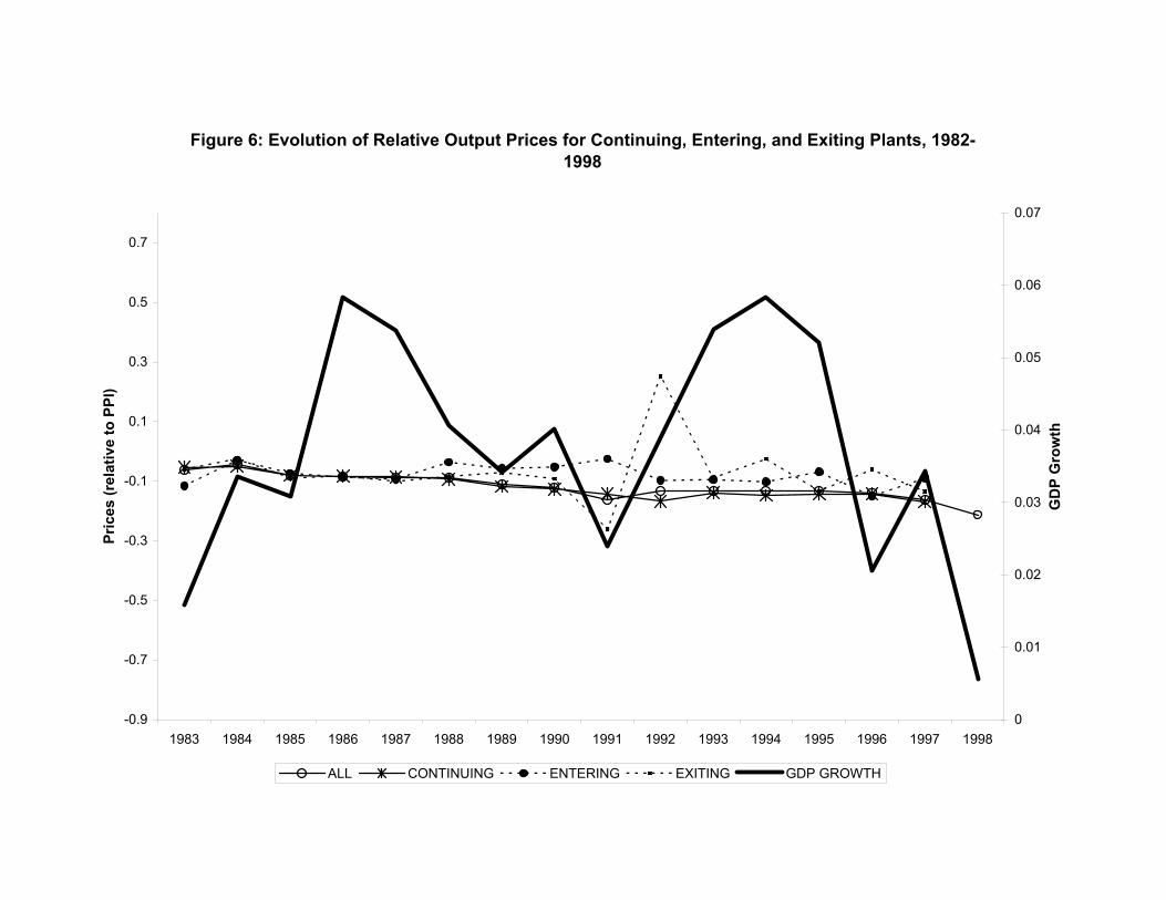
Figure 6: Evolution of Relative Output Prices for Continuing, Entering, and Exiting Plants, 1982-1998

-0.9

-0.7

-0.5

-0.3

-0.1

0.1

0.3

0.5

0.7

1983 1984 1985 1986 1987 1988 1989 1990 1991 1992 1993 1994 1995 1996 1997 1998

Pric

es (r

elat

ive

to P

PI)

0

0.01

0.02

0.03

0.04

0.05

0.06

0.07

GD

P G

row

th

ALL CONTINUING ENTERING EXITING GDP GROWTH

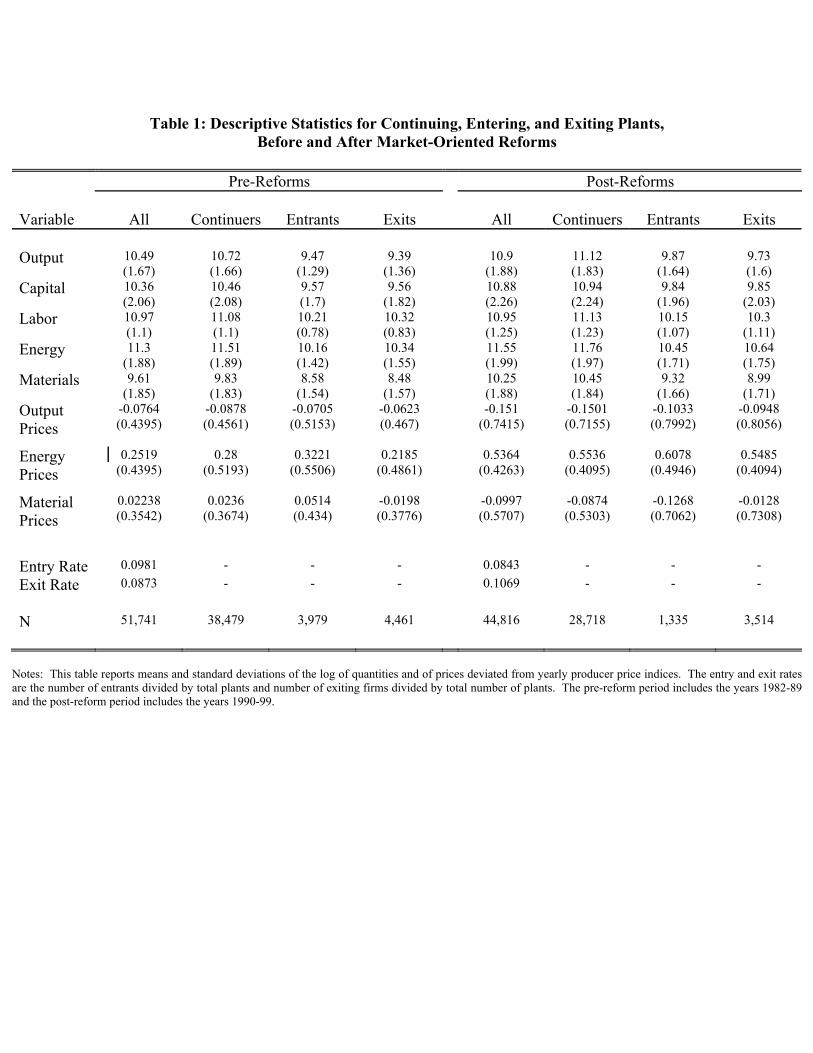
Table 1: Descriptive Statistics for Continuing, Entering, and Exiting Plants,

Before and After Market-Oriented Reforms

Pre-Reforms Post-Reforms

Variable All Continuers Entrants Exits All Continuers Entrants Exits Output 10.49

(1.67) 10.72 (1.66)

9.47 (1.29)

9.39 (1.36)

10.9 (1.88)

11.12 (1.83)

9.87 (1.64)

9.73 (1.6)

Capital 10.36 (2.06)

10.46 (2.08)

9.57 (1.7)

9.56 (1.82)

10.88 (2.26)

10.94 (2.24)

9.84 (1.96)

9.85 (2.03)

Labor 10.97 (1.1)

11.08 (1.1)

10.21 (0.78)

10.32 (0.83)

10.95 (1.25)

11.13 (1.23)

10.15 (1.07)

10.3 (1.11)

Energy 11.3 (1.88)

11.51 (1.89)

10.16 (1.42)

10.34 (1.55)

11.55 (1.99)

11.76 (1.97)

10.45 (1.71)

10.64 (1.75)

Materials 9.61 (1.85)

9.83 (1.83)

8.58 (1.54)

8.48 (1.57)

10.25 (1.88)

10.45 (1.84)

9.32 (1.66)

8.99 (1.71)

Output Prices

-0.0764 (0.4395)

-0.0878 (0.4561)

-0.0705 (0.5153)

-0.0623 (0.467)

-0.151 (0.7415)

-0.1501 (0.7155)

-0.1033 (0.7992)

-0.0948 (0.8056)

Energy Prices

0.2519 (0.4395)

0.28 (0.5193)

0.3221 (0.5506)

0.2185 (0.4861)

0.5364 (0.4263)

0.5536 (0.4095)

0.6078 (0.4946)

0.5485 (0.4094)

Material Prices

0.02238 (0.3542)

0.0236 (0.3674)

0.0514 (0.434)

-0.0198 (0.3776)

-0.0997 (0.5707)

-0.0874 (0.5303)

-0.1268 (0.7062)

-0.0128 (0.7308)

Entry Rate 0.0981 - - - 0.0843 - - - Exit Rate 0.0873 - - - 0.1069 - - - N 51,741 38,479 3,979 4,461 44,816 28,718 1,335 3,514

Notes: This table reports means and standard deviations of the log of quantities and of prices deviated from yearly producer price indices. The entry and exit rates are the number of entrants divided by total plants and number of exiting firms divided by total number of plants. The pre-reform period includes the years 1982-89 and the post-reform period includes the years 1990-99.

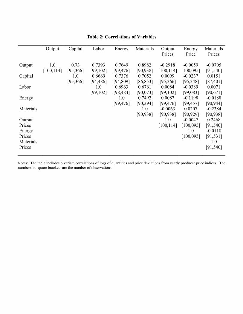
Table 2: Correlations of Variables

Output Capital Labor Energy Materials Output

Prices Energy Price

Materials Prices

Output

1.0 [100,114]

0.73 [95,366]

0.7393 [99,102]

0.7649 [99,476]

0.8982 [90,938]

-0.2918 [100,114]

-0.0059 [100,095]

-0.0705 [91,540]

Capital

1.0 [95,366]

0.6669 [94,486]

0.7376 [94,809]

0.7052 [86,853]

0.0099 [95,366]

-0.0237 [95,348]

0.0151 [87,401]

Labor

1.0 [99,102]

0.6963 [98,484]

0.6761 [90,073]

0.0084 [99,102]

-0.0389 [99,083]

0.0071 [90,671]

Energy

1.0 [99,476]

0.7492 [90,394]

0.0087 [99,476]

-0.1198 [99,457]

-0.0188 [90,944]

Materials

1.0 [90,938]

-0.0063 [90,938]

0.0207 [90,929]

-0.2384 [90,938]

Output Prices

1.0 [100,114]

-0.0047 [100,095]

0.2468 [91,540]

Energy Prices

1.0 [100,095]

-0.0118 [91,531]

Materials Prices

1.0 [91,540]

Notes: The table includes bivariate correlations of logs of quantities and price deviations from yearly producer price indices. The numbers in square brackets are the number of observations.

Table 3: Production Function Equations

OLS 2SLS (1) (2) (3) (4) Capital 0.2618

(0.004) 0.0602 (0.002)

0.3053 (0.0114)

0.0509 (0.0127)

Labor 0.8116 (0.006)

- 0.8156 (0.0303)

Labor hours - 0.2503 (0.003)

- 0.441 (0.0163)

Energy - 0.1259 (0.0025)

- 0.2184 (0.0094)

Materials - 0.5964 (0.0023)

- 0.4023 (0.0063)

R² 0.5870 0.8727 0.5888 0.8522 N 48,240 54,635 48,990 54,635

Notes: The standard errors are reported in parentheses. The regressions in Columns (1) and (3) use the log of value added as the dependent variable, where value added is revenue minus materials and energy costs. The regressions in Columns (2) and (4) use the log of physical output as the dependent variable. All regressors are in logs. The two-stage least squares regressions use the following variables to instrument the inputs: Shea’s (1993) downstream demand instruments constructed as the demand for the intermediate output constructed using the input-output matrix; downstream demand squared; downstream demand cubed; downstream demand to the fourth power; one- and two-period lags of downstream demand; regional GDP; and firm-level, yearly, regional, and sectoral energy and material prices.

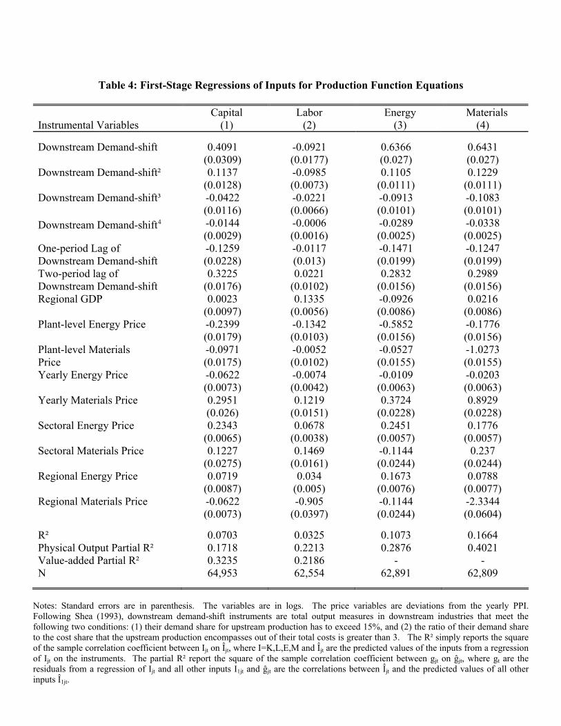
Table 4: First-Stage Regressions of Inputs for Production Function Equations

Capital Labor Energy Materials Instrumental Variables (1) (2) (3) (4) Downstream Demand-shift 0.4091

(0.0309) -0.0921 (0.0177)

0.6366 (0.027)

0.6431 (0.027)

Downstream Demand-shift² 0.1137 (0.0128)

-0.0985 (0.0073)

0.1105 (0.0111)

0.1229 (0.0111)

Downstream Demand-shift³ -0.0422 (0.0116)

-0.0221 (0.0066)

-0.0913 (0.0101)

-0.1083 (0.0101)

Downstream Demand-shift$ -0.0144 (0.0029)

-0.0006 (0.0016)

-0.0289 (0.0025)

-0.0338 (0.0025)

One-period Lag of Downstream Demand-shift

-0.1259 (0.0228)

-0.0117 (0.013)

-0.1471 (0.0199)

-0.1247 (0.0199)

Two-period lag of Downstream Demand-shift

0.3225 (0.0176)

0.0221 (0.0102)

0.2832 (0.0156)

0.2989 (0.0156)

Regional GDP 0.0023 (0.0097)

0.1335 (0.0056)

-0.0926 (0.0086)

0.0216 (0.0086)

Plant-level Energy Price -0.2399 (0.0179)

-0.1342 (0.0103)

-0.5852 (0.0156)

-0.1776 (0.0156)

Plant-level Materials Price

-0.0971 (0.0175)

-0.0052 (0.0102)

-0.0527 (0.0155)

-1.0273 (0.0155)

Yearly Energy Price -0.0622 (0.0073)

-0.0074 (0.0042)

-0.0109 (0.0063)

-0.0203 (0.0063)

Yearly Materials Price 0.2951 (0.026)

0.1219 (0.0151)

0.3724 (0.0228)

0.8929 (0.0228)

Sectoral Energy Price 0.2343 (0.0065)

0.0678 (0.0038)

0.2451 (0.0057)

0.1776 (0.0057)

Sectoral Materials Price 0.1227 (0.0275)

0.1469 (0.0161)

-0.1144 (0.0244)

0.237 (0.0244)

Regional Energy Price 0.0719 (0.0087)

0.034 (0.005)

0.1673 (0.0076)

0.0788 (0.0077)

Regional Materials Price -0.0622 (0.0073)

-0.905 (0.0397)

-0.1144 (0.0244)

-2.3344 (0.0604)

R² 0.0703 0.0325 0.1073 0.1664 Physical Output Partial R² 0.1718 0.2213 0.2876 0.4021 Value-added Partial R² 0.3235 0.2186 - - N 64,953 62,554 62,891 62,809

Notes: Standard errors are in parenthesis. The variables are in logs. The price variables are deviations from the yearly PPI. Following Shea (1993), downstream demand-shift instruments are total output measures in downstream industries that meet the following two conditions: (1) their demand share for upstream production has to exceed 15%, and (2) the ratio of their demand share to the cost share that the upstream production encompasses out of their total costs is greater than 3. The R² simply reports the square of the sample correlation coefficient between Ijt on Îjt, where I=K,L,E,M and Îjt are the predicted values of the inputs from a regression of Ijt on the instruments. The partial R² report the square of the sample correlation coefficient between gjt on ĝjt, where gt are the residuals from a regression of Ijt and all other inputs I1jt and ĝjt are the correlations between Îjt and the predicted values of all other inputs Î1jt.

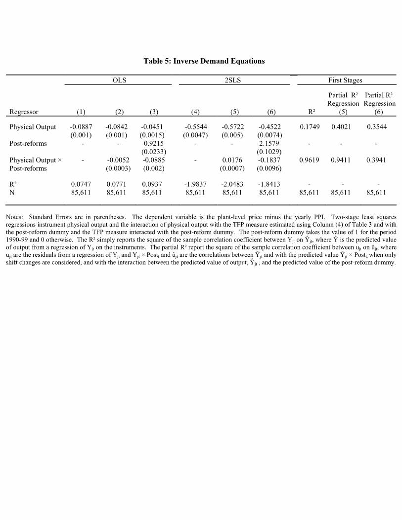
Table 5: Inverse Demand Equations

OLS 2SLS First Stages

Regressor

(1)

(2)

(3)

(4)

(5)

(6)

R²

Partial R² Regression

(5)

Partial R² Regression

(6)

Physical Output -0.0887 (0.001)

-0.0842 (0.001)

-0.0451 (0.0015)

-0.5544 (0.0047)

-0.5722 (0.005)

-0.4522 (0.0074)

0.1749 0.4021 0.3544

Post-reforms

- - 0.9215 (0.0233)

- - 2.1579 (0.1029)

- - -

Physical Output × Post-reforms

- -0.0052 (0.0003)

-0.0885 (0.002)

- 0.0176 (0.0007)

-0.1837 (0.0096)

0.9619 0.9411 0.3941

R² 0.0747 0.0771 0.0937 -1.9837 -2.0483 -1.8413 - - - N 85,611 85,611 85,611 85,611 85,611 85,611 85,611 85,611 85,611

Notes: Standard Errors are in parentheses. The dependent variable is the plant-level price minus the yearly PPI. Two-stage least squares regressions instrument physical output and the interaction of physical output with the TFP measure estimated using Column (4) of Table 3 and with the post-reform dummy and the TFP measure interacted with the post-reform dummy. The post-reform dummy takes the value of 1 for the period 1990-99 and 0 otherwise. The R² simply reports the square of the sample correlation coefficient between Yjt on Ŷjt, where Ŷ is the predicted value of output from a regression of Yjt on the instruments. The partial R² report the square of the sample correlation coefficient between ujt on ûjt, where ujt are the residuals from a regression of Yjt and Yjt × Postt and ûjt are the correlations between Ŷjt and with the predicted value Ŷjt × Postt, when only shift changes are considered, and with the interaction between the predicted value of output, Ŷjt , and the predicted value of the post-reform dummy.

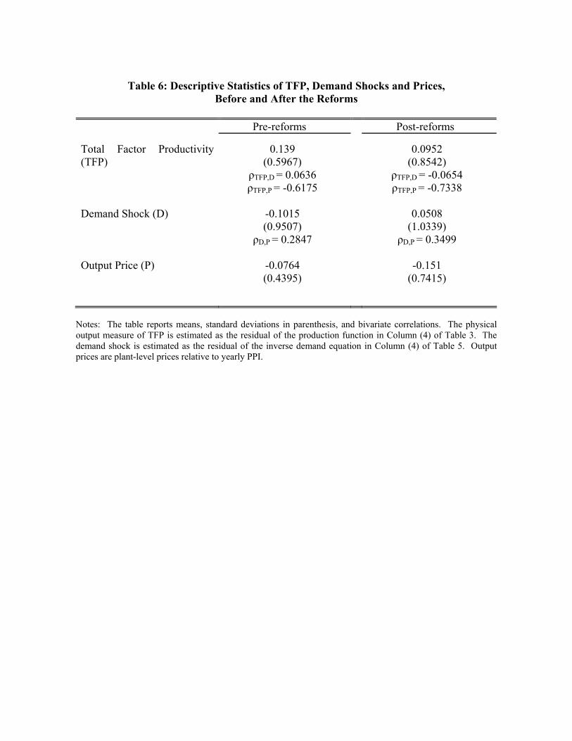
Table 6: Descriptive Statistics of TFP, Demand Shocks and Prices,

Before and After the Reforms

Pre-reforms Post-reforms Total Factor Productivity (TFP)

0.139 (0.5967)

ρTFP,D = 0.0636 ρTFP,P = -0.6175

0.0952 (0.8542)

ρTFP,D = -0.0654 ρTFP,P = -0.7338

Demand Shock (D) -0.1015

(0.9507) ρD,P = 0.2847

0.0508 (1.0339)

ρD,P = 0.3499

Output Price (P) -0.0764 (0.4395)

-0.151 (0.7415)

Notes: The table reports means, standard deviations in parenthesis, and bivariate correlations. The physical output measure of TFP is estimated as the residual of the production function in Column (4) of Table 3. The demand shock is estimated as the residual of the inverse demand equation in Column (4) of Table 5. Output prices are plant-level prices relative to yearly PPI.

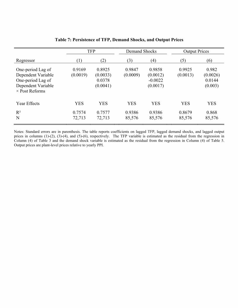
Table 7: Persistence of TFP, Demand Shocks, and Output Prices

TFP Demand Shocks Output Prices Regressor (1) (2) (3) (4) (5) (6) One-period Lag of Dependent Variable

0.9169 (0.0019)

0.8925 (0.0033)

0.9847 (0.0009)

0.9858 (0.0012)

0.9925 (0.0013)

0.982 (0.0026)

One-period Lag of Dependent Variable × Post Reforms

0.0378 (0.0041)

-0.0022 (0.0017)

0.0144 (0.003)

Year Effects YES YES YES YES YES YES R² 0.7574 0.7577 0.9386 0.9386 0.8679 0.868 N 72,713 72,713 85,576 85,576 85,576 85,576

Notes: Standard errors are in parenthesis. The table reports coefficients on lagged TFP, lagged demand shocks, and lagged output prices in columns (1)-(2), (3)-(4), and (5)-(6), respectively. The TFP variable is estimated as the residual from the regression in Column (4) of Table 3 and the demand shock variable is estimated as the residual from the regression in Column (4) of Table 5. Output prices are plant-level prices relative to yearly PPI.

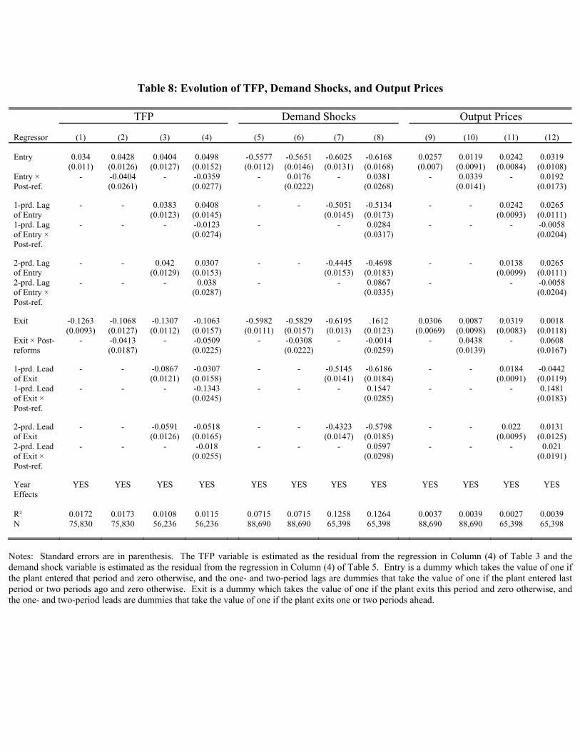
Table 8: Evolution of TFP, Demand Shocks, and Output Prices

TFP Demand Shocks Output Prices

Regressor (1) (2) (3) (4) (5) (6) (7) (8) (9) (10) (11) (12) Entry 0.034

(0.011) 0.0428

(0.0126) 0.0404

(0.0127) 0.0498

(0.0152) -0.5577

(0.0112) -0.5651 (0.0146)

-0.6025 (0.0131)

-0.6168 (0.0168)

0.0257 (0.007)

0.0119 (0.0091)

0.0242 (0.0084)

0.0319 (0.0108)

Entry × Post-ref.

- -0.0404 (0.0261)

- -0.0359 (0.0277)

- 0.0176 (0.0222)

- 0.0381 (0.0268)

- 0.0339 (0.0141)

- 0.0192 (0.0173)

1-prd. Lag of Entry

- - 0.0383 (0.0123)

0.0408 (0.0145)

- - -0.5051 (0.0145)

-0.5134 (0.0173)

- - 0.0242 (0.0093)

0.0265 (0.0111)

1-prd. Lag of Entry × Post-ref.

- - - -0.0123 (0.0274)

- - 0.0284 (0.0317)

- - - -0.0058 (0.0204)

2-prd. Lag of Entry

- - 0.042 (0.0129)

0.0307 (0.0153)

- - -0.4445 (0.0153)

-0.4698 (0.0183)

- - 0.0138 (0.0099)

0.0265 (0.0111)

2-prd. Lag of Entry × Post-ref.

- - - 0.038 (0.0287)

- - 0.0867 (0.0335)

- - -0.0058 (0.0204)

Exit -0.1263

(0.0093) -0.1068 (0.0127)

-0.1307 (0.0112)

-0.1063 (0.0157)

-0.5982 (0.0111)

-0.5829 (0.0157)

-0.6195 (0.013)

.1612 (0.0123)

0.0306 (0.0069)

0.0087 (0.0098)

0.0319 (0.0083)

0.0018 (0.0118)

Exit × Post-reforms

- -0.0413 (0.0187)

- -0.0509 (0.0225)

- -0.0308 (0.0222)

- -0.0014 (0.0259)

- 0.0438 (0.0139)

- 0.0608 (0.0167)

1-prd. Lead of Exit

- - -0.0867 (0.0121)

-0.0307 (0.0158)

- - -0.5145 (0.0141)

-0.6186 (0.0184)

- - 0.0184 (0.0091)

-0.0442 (0.0119)

1-prd. Lead of Exit × Post-ref.

- - - -0.1343 (0.0245)

- - - 0.1547 (0.0285)

- - - 0.1481 (0.0183)

2-prd. Lead of Exit

- - -0.0591 (0.0126)

-0.0518 (0.0165)

- - -0.4323 (0.0147)

-0.5798 (0.0185)

- - 0.022 (0.0095)

0.0131 (0.0125)

2-prd. Lead of Exit × Post-ref.

- - - -0.018 (0.0255)

- - - 0.0597 (0.0298)

- - - 0.021 (0.0191)

Year Effects

YES YES YES YES YES YES YES YES YES YES YES YES

R² 0.0172 0.0173 0.0108 0.0115 0.0715 0.0715 0.1258 0.1264 0.0037 0.0039 0.0027 0.0039 N 75,830 75,830 56,236 56,236 88,690 88,690 65,398 65,398 88,690 88,690 65,398 65,398

Notes: Standard errors are in parenthesis. The TFP variable is estimated as the residual from the regression in Column (4) of Table 3 and the demand shock variable is estimated as the residual from the regression in Column (4) of Table 5. Entry is a dummy which takes the value of one if the plant entered that period and zero otherwise, and the one- and two-period lags are dummies that take the value of one if the plant entered last period or two periods ago and zero otherwise. Exit is a dummy which takes the value of one if the plant exits this period and zero otherwise, and the one- and two-period leads are dummies that take the value of one if the plant exits one or two periods ahead.

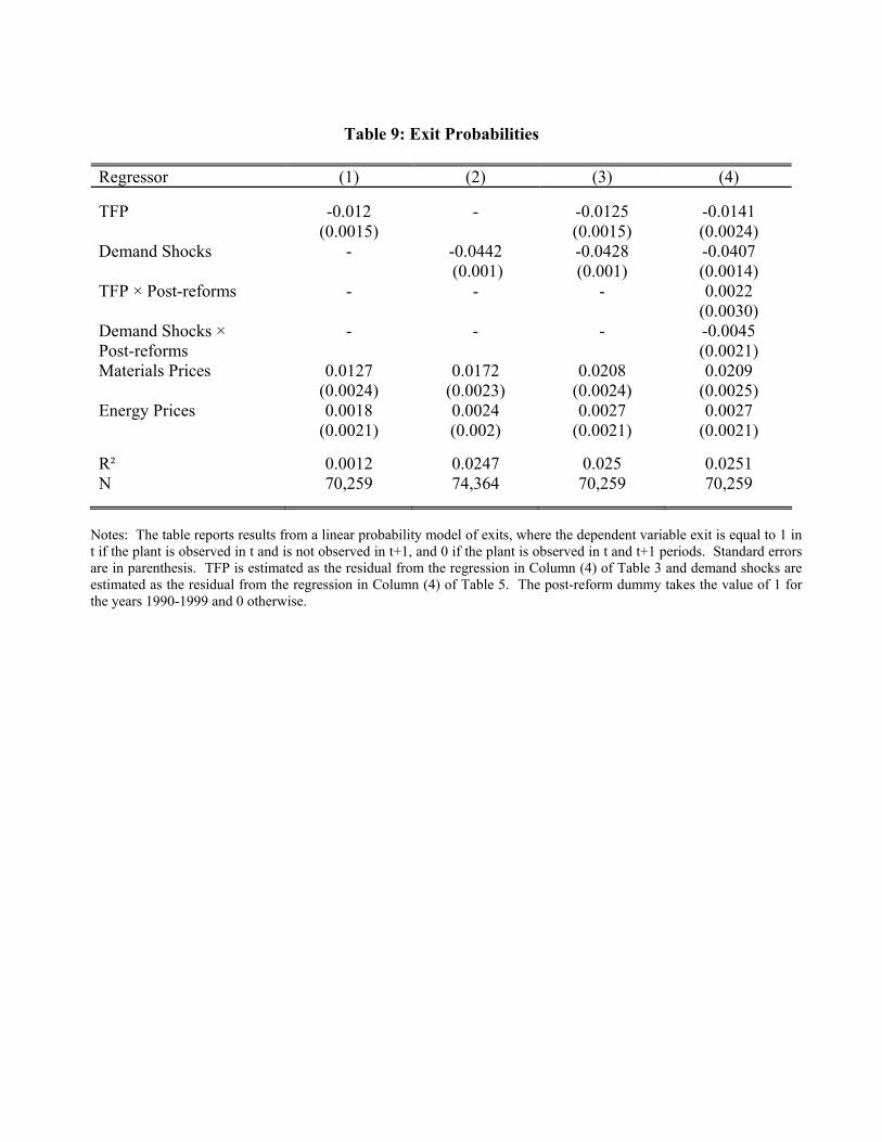
Table 9: Exit Probabilities

Regressor (1) (2) (3) (4) TFP -0.012

(0.0015) - -0.0125

(0.0015) -0.0141 (0.0024)

Demand Shocks - -0.0442 (0.001)

-0.0428 (0.001)

-0.0407 (0.0014)

TFP × Post-reforms - - - 0.0022 (0.0030)

Demand Shocks × Post-reforms

- - - -0.0045 (0.0021)

Materials Prices 0.0127 (0.0024)

0.0172 (0.0023)

0.0208 (0.0024)

0.0209 (0.0025)

Energy Prices 0.0018 (0.0021)

0.0024 (0.002)

0.0027 (0.0021)

0.0027 (0.0021)

R² 0.0012 0.0247 0.025 0.0251 N 70,259 74,364 70,259 70,259

Notes: The table reports results from a linear probability model of exits, where the dependent variable exit is equal to 1 in t if the plant is observed in t and is not observed in t+1, and 0 if the plant is observed in t and t+1 periods. Standard errors are in parenthesis. TFP is estimated as the residual from the regression in Column (4) of Table 3 and demand shocks are estimated as the residual from the regression in Column (4) of Table 5. The post-reform dummy takes the value of 1 for the years 1990-1999 and 0 otherwise.