
The Natural Space Environment: Effects on Spacecraft
30
The Natural Space Environment: Effects on Spacecraft NASA Reference Publication 1350 November 1994 Bonnie F. James, Coordinator O.W. Norton, Compiler, and Margaret B. Alexander, Editor 5-21957 Neutral Thermosphere Thermal Environment Plasma Plasma Plasma Meteoroid/ Orbital Debris Neutral Thermosphere Thermal Environment Meteoroid/ Orbital Debris Neutral Thermosphere Thermal Environment Meteoroid/ Orbital Debris Solar Environment Ionizing Radiation Geomagnetic Field Gravitational Field Solar Environment Ionizing Radiation Geomagnetic Field Gravitational Field Solar Environment Ionizing Radiation Geomagnetic Field Gravitational Field T h e N a t u r a l S p a c e E n v i r o n m e n t s T h e N a t u r a l S p a c e E n v i r o n m e n t s Downloaded from http://www.everyspec.com
Transcript of The Natural Space Environment: Effects on Spacecraft

The Natural Space Environment:Effects on Spacecraft
NASA Reference Publication 1350
November 1994
Bonnie F. James, CoordinatorO.W. Norton, Compiler, andMargaret B. Alexander, Editor
5-21957
������
����
Neutral Thermosphere
Thermal Environment
Plasma
Plasma
Plasma
Meteoroid/
Orbital Debris
Neutral Thermosphere
Thermal Environment
Meteoroid/
Orbital Debris
Neutral Thermosphere
Thermal Environment
Meteoroid/
Orbital Debris
����
����
Solar Environment
Ionizing Radiation
Geomagnetic
Field
Gravitational Field
Solar Environment
Ionizing Radiation
Geomagnetic
Field
Gravitational Field
Solar Environment
Ionizing Radiation
Geomagnetic
Field
Gravitational Field
The
Natu
ral Space
Envir
on
m
ents
The
Natu
ral Spac
e
Envir
on
m
ents
Downloaded from http://www.everyspec.com
The Natural Space Environment:Effects on Spacecraft
National Aeronautics and Space AdministrationMarshall Space Flight Center • MSFC, Alabama 35812
NASA Reference Publication 1350
November 1994
Bonnie F. James, CoordinatorO.W. Norton, Compiler, andMargaret B. Alexander, EditorMarshall Space Flight Center • MSFC, Alabama
Prepared byElectromagnetics and Environments BranchSystems Definition DivisionSystems Analysis and Integration LaboratoryScience and Engineering Directorate
Downloaded from http://www.everyspec.com

ii
PREFACE
The effects of the natural space environment on spacecraft design, development, andoperations are the topic of a series of NASA Reference Publications currently being developed by theElectromagnetics and Environments Branch, Systems Analysis and Integration Laboratory,Marshall Space Flight Center.
This primer provides an overview of the natural space environment and its effects onspacecraft design, development, and operations, and also highlights some of the new developmentsin science and technology for natural space environment. It is hoped that a better understanding ofthe space environment and its effects on spacecraft will enable program management to moreeffectively minimize program risks and costs, optimize design quality, and successfully achievemission objectives.
Downloaded from http://www.everyspec.com

iii
TABLE OF CONTENTS
Page
INTRODUCTION 1
NEUTRAL THERMOSPHERE 5
THERMAL ENVIRONMENT 8
PLASMA 11
METEOROID/ORBITAL DEBRIS 15
SOLAR ENVIRONMENT 18
IONIZING RADIATION 20
GEOMAGNETIC FIELD 22
GRAVITATIONAL FIELD 24
CONCLUSION 25
Downloaded from http://www.everyspec.com

iv
LIST OF ACRONYMS
AO atomic oxygen
CRRES combined release and radiation effects satellite
DMSP defense meteorological satellite program
EMI electromagnetic interference
ERBE Earth radiation budget experiment
EUV extreme ultraviolet
GCM general circulation model
GCR galactic cosmic rays
GN&C guidance, navigation, and control
IGRF international geomagnetic reference field
IRI international reference ionosphere
LEO low-Earth orbit
MET Marshall engineering thermosphere
M/OD meteoroid/orbital debris
MSFC Marshall Space Flight Center
MSIS mass spectrometer incoherent scatter
NASA National Aeronautics and Space Administration
NOAA National Oceanic and Atmospheric Administration
NORAD North American Air Defense Command
OLR outgoing long-wave radiation
POLAR potential of large spacecraft in auroral regions (computer model)
SAMPEX solar, anomalous, and magnetospheric particle explorer
S/C spacecraft
SAA South Atlantic anomaly
UV ultraviolet
Downloaded from http://www.everyspec.com

REFERENCE PUBLICATION
THE NATURAL SPACE ENVIRONMENT: EFFECTS ON SPACECRAFT
INTRODUCTION
The natural space environment refers to the environment as it occurs independent of thepresence of a spacecraft; thus, it includes both naturally occurring phenomena such as atomic oxygen(AO) and atmospheric density, ionizing radiation, plasma, etc., and a few man-made factors such asorbital debris. Figures 1 through 3 list the breakout of the natural space environments and theirmajor areas of interaction with spacecraft systems.
This primer provides an overview of these natural space environments and their effect onspacecraft design, development, and operations, and it also highlights some of the new devel-opments in science and technology for each space environment.
Understanding these natural space environments and their effect on spacecraft enables pro-gram management to more effectively optimize the following aspects of a spacecraft mission:
• Risk—Increasingly, experience on past missions is enabling NASA to provide statisticaldescriptions of important environmental factors, thus enabling the manager to make informeddecisions on design options.
• Cost—Selection of design concepts and missions profiles, especially orbit inclination and altitudewhich minimizes adverse environmental impacts, is the first important step toward a simple,effective, high-quality spacecraft design and low operational costs.
• Quality—New environment simulators and models provide effective tools for optimizing sub-system designs and mission operations.
• Weight—Consideration of environmental effects early in the mission design cycle helps to mini-mize weight impacts at later stages. For example, early consideration of directionality effects inthe orbital debris and ionizing radiation environments could lead to reduced shielding weights.
• Verification—A unified, complete environments description coupled with a clear mission profileprovides a sound basis for analysis and test requirements in the verification process and elimi-nates contradictory, unnecessary, and/or incomplete performance assessments.
• Science and Technology—The natural space environment is not static. Not only is our under-standing improving, but new things occur in nature which have not been observed before (forexample, a new transient radiation belt was recently encountered). Perhaps more importantly,engineering technology is constantly changing and with this the susceptibility of spacecraft toenvironmental factors. Early consideration of these factors is key to converging quickly on aquality system design and to successfully achieving mission objectives.
Downloaded from http://www.everyspec.com

2
Nat
ura
l Sp
ace
En
viro
nm
ents
NE
UT
RA
L
TH
ER
MO
SP
HE
RE
TH
ER
MA
L
EN
VIR
ON
ME
NT
PL
AS
MA
ME
TE
OR
OID
S A
ND
O
RB
ITA
L D
EB
RIS
SO
LA
R E
NV
IRO
NM
EN
T
ION
IZIN
G R
AD
IAT
ION
MA
GN
ET
IC F
IEL
D
GR
AV
ITA
TIO
NA
L F
IEL
D
ME
SO
SP
HE
RE
GN
&C
sys
tem
des
ign,
Mat
eria
ls d
egra
datio
n/
surf
ace
eros
ion
(ato
mic
oxy
gen
fluen
ces)
, D
rag/
deca
y, S
/C li
fetim
e, C
ollis
ion
avoi
danc
e,
Sen
sor
poin
ting,
Exp
erim
ent d
esig
n, O
rbita
l po
sitio
nal e
rror
s, T
rack
ing
loss
Pas
sive
and
act
ive
ther
mal
con
trol
sys
tem
de
sign
, Rad
iato
r si
zing
/mat
eria
l sel
ectio
n,
Pow
er a
lloca
tion,
Sol
ar a
rray
des
ign
EM
I, S
/C p
ower
sys
tem
s de
sign
, m
ater
ial d
eter
min
atio
n, S
/C h
eatin
g,
S/C
cha
rgin
g/ar
cing
Col
lisio
n av
oida
nce,
Cre
w s
urvi
vabi
lity,
S
econ
ary
ejec
ta e
ffect
s, S
truc
tura
l des
ign/
sh
ield
ing,
Mat
eria
ls/s
olar
pan
el d
eter
iora
tion
Sol
ar p
redi
ctio
n, L
ifetim
e/dr
ag a
sses
smen
ts,
Ree
ntry
load
s/he
atin
g, In
put f
or o
ther
m
odel
s, C
ontin
genc
y op
erat
ions
Rad
iatio
n le
vels
, Ele
ctro
nics
/par
ts d
ose,
E
lect
roni
cs/s
ingl
e ev
ent u
pset
, Mat
eria
ls
dose
leve
ls, H
uman
dos
e le
vels
Indu
ced
curr
ents
in la
rge
stru
ctur
es,
Loca
ting
Sou
th A
tlant
ic A
nom
aly,
Loc
atio
n of
ra
diat
ion
belts
Orb
ital m
echa
nics
/trac
king
Re-
entr
y, M
ater
ials
sel
ectio
n,
Tet
her
expe
rimen
t des
ign
Figu
re 1
. A
bre
akou
t of
the
natu
ral S
pace
env
iron
men
ts a
nd ty
pica
l pro
gram
mat
ic c
once
rns.
DE
FIN
ITIO
NP
RO
GR
AM
MA
TIC
ISS
UE
SM
OD
EL
S/D
AT
AB
AS
ES
MS
FC
EM
& E
nviro
nmen
ts B
ranc
h/E
L54
Atm
osph
eric
den
sity
, Den
sity
va
riatio
ns,
Atm
osph
eric
com
posi
tion
(Ato
mic
Oxy
gen)
, Win
ds
Sol
ar r
adia
tion
(alb
edo
and
OLR
var
iatio
ns),
R
adia
tive
tran
sfer
, Atm
osph
eric
tr
ansm
ittan
ce
Iono
sphe
ric p
lasm
a,
Aur
oral
pla
sma,
Mag
neto
sphe
ric
plas
ma
M/O
D fl
ux, S
ize
dist
ribut
ion,
M
ass
dist
ribut
ion,
Vel
ocity
di
strib
utio
n, D
irect
iona
lity
Sol
ar p
hysi
cs a
nd d
ynam
ics,
G
eom
etric
sto
rms,
Sol
ar a
ctiv
ity
pred
ictio
ns, S
olar
/geo
mag
netic
in
dice
s, S
olar
con
stan
t, S
olar
spe
ctru
m
Tra
pped
pro
ton/
elec
tron
rad
iatio
n,
Gal
actic
cos
mic
ray
s (G
CR
’s),
S
olar
par
ticle
eve
nts
Nat
ural
mag
netic
fiel
d
Nat
ural
gra
vita
tiona
l fie
ld
Atm
osph
eric
den
sity
, Den
sity
va
riatio
ns, W
inds
Jacc
hia/
ME
T, M
SIS
< L
IFT
IM, u
pper
at
mos
pher
ic w
ind
mod
els
ER
BE
dat
abas
e, E
RB
dat
abas
e,
NIM
BU
S d
atab
ase,
ISS
CP
da
taba
se, C
limat
e m
odel
s,
Gen
eral
Circ
ulat
ion
Mod
els
(GC
M’s
)
Inte
rnat
iona
l Ref
eren
ce
Iono
sphe
re M
odel
s, N
AS
CA
P/L
EO
N
AS
CA
P/G
EO
, PO
LAR
Flu
x m
odel
s
EL
Labo
rato
ry m
odel
, NO
AA
pr
edic
tion
data
, Sta
tistic
al
mod
els,
Sol
ar d
atab
ase
CR
EM
E, A
E-8
MIN
, A
E-8
MA
X, A
P-8
MIN
, A
P-8
MA
X, R
adbe
lt, S
olpr
o,
SH
IELD
OS
E
IGR
F85
, IG
RF
91
GE
M-T
1, G
EM
-T2
Ear
th-G
RA
M 9
0, U
AR
S d
atab
ase,
“s
cien
ce”
GR
AM
Downloaded from http://www.everyspec.com

3
Sp
ace
En
viro
nm
ent
Eff
ects
Figu
re 2
. Sp
ace
envi
ronm
ent e
ffec
ts o
n sp
acec
raft
sub
syst
ems.
SP
AC
EC
RA
FT
S
UB
SY
ST
EM
S
Avi
on
ics
Ele
ctri
cal P
ow
er
GN
&C
/Po
inti
ng
Mat
eria
ls
Op
tics
Pro
pu
lsio
n
Str
uct
ure
s
Tel
emet
ry,
Tra
ckin
g, a
nd
C
om
mu
nic
atio
ns
Th
erm
al C
on
tro
l
Mis
sio
n
Op
erat
ion
s
Neu
tral
Th
erm
osp
her
eT
her
mal
En
viro
nm
ent
Pla
sma
Met
eoro
ids/
Orb
ital
Deb
ris
SP
AC
E E
NV
IRO
NM
EN
TS
MS
FC
EM
& E
nviro
nmen
ts B
ranc
h/E
L54
Deg
rada
tion
of S
olar
Arr
ay
Per
form
ance
Ove
rall
GN
&C
/Poi
ntin
g S
yste
m
Des
ign
Mat
eria
l Sel
ectio
n, M
ater
ial
Deg
rada
tion
S/C
Glo
w, I
nter
fere
nce
with
S
enso
rs
Dra
g M
akeu
p/F
uel R
equi
rem
ent
Pos
sibl
e T
rack
ing
Err
ors,
Pos
sibl
e T
rack
ing
Loss
Ree
ntry
Loa
ds/H
eatin
g, S
urfa
ce
Deg
rada
tion
due
to A
tom
ic
Oxy
gen
Reb
oost
Tim
elin
es, S
/C L
ifetim
e A
sses
smen
t
The
rmal
Des
ign
Sol
ar A
rray
Des
igns
, Pow
er
Allo
catio
ns, P
ower
Sys
tem
P
erfo
rman
ce
Mat
eria
l S
elec
tion
Influ
ence
s O
ptic
al D
esig
n
Influ
ence
s P
lace
men
t of
The
rmal
ly S
ensi
tive
Sur
face
s,
Fat
igue
, The
rmal
ly In
duce
d V
ibra
tions
Pas
sive
and
Act
ive
The
rmal
C
ontr
ol S
yste
m D
esig
n, R
adia
tor
Siz
ing,
Fre
ezin
g P
oint
s
Influ
ence
s M
issi
on P
lann
ing/
S
eque
ncin
g
Ups
ets
due
to E
MI f
rom
A
rcin
g, S
/C C
harg
ing
Shi
ft in
Flo
atin
g P
oten
tial,
Cur
rent
Los
ses,
R
eattr
actio
n of
Con
tam
inan
ts
Tor
ques
due
to In
duce
d P
oten
tial
Arc
ing,
Spu
tterin
g,
Con
tam
inat
ion
Effe
cts
on S
urfa
ce P
rope
rtie
s R
eattr
actio
n of
Con
tam
inan
ts,
Cha
nge
in S
urfa
ce O
ptic
al
Pro
pert
ies
Shi
ft in
Flo
atin
g P
oten
tial D
ue
to T
hrus
ter
Firi
ngs
mak
ing
Con
tact
with
the
Pla
sma
Mas
s Lo
ss F
rom
Arc
ing
and
Spu
tterin
g, S
truc
tura
l Siz
e In
fluen
ces
S/C
Cha
rgin
g E
ffect
s
EM
I Due
to A
rcin
g
Rea
ttrac
tion
of C
onta
min
ants
, C
hang
e in
abs
orpt
ance
/ em
ittan
ce p
rope
rtie
s
Ser
vici
ng (
EV
A)
Tim
elin
es
EM
I Due
to Im
pact
s
Dam
age
to S
olar
Cel
ls
Col
lisio
n A
void
ance
Deg
rada
tion
of S
urfa
ce
Opt
ical
Pro
pert
ies
Deg
rada
tion
of S
urfa
ce
Opt
ical
Pro
pert
ies
Col
lisio
n A
void
ance
, Add
ition
al
Shi
eldi
ng In
crea
ses
Fue
l Req
uire
men
t, R
uptu
re o
f Pre
ssur
ized
Tan
ks
Str
uctu
ral D
amag
e, S
hiel
ding
Des
igns
, O
vera
ll S
/C W
eigh
t, C
rew
Sur
viva
bilit
y
EM
I Due
to Im
pact
s
Cha
nge
in T
herm
al/O
ptic
al P
rope
rtie
s
Cre
w S
urvi
vabi
lity
Downloaded from http://www.everyspec.com

4
Sp
ace
En
viro
nm
ent
Eff
ects
Figu
re 3
. Sp
ace
envi
ronm
ent e
ffec
ts o
n sp
acec
raft
sub
syst
ems.
SP
AC
EC
RA
FT
S
UB
SY
ST
EM
S
Avi
on
ics
Ele
ctri
cal P
ow
er
GN
&C
/Po
inti
ng
Mat
eria
ls
Op
tics
Pro
pu
lsio
n
Str
uct
ure
s
Tel
emet
ry,
Tra
ckin
g a
nd
C
om
mu
nic
atio
n
Th
erm
al C
on
tro
l
Mis
sio
n
Op
erat
ion
s
SP
AC
E E
NV
IRO
NM
EN
TS
So
lar
En
viro
nm
ent
Ion
izin
g R
adia
tio
nM
agn
etic
Fie
ldG
ravi
tati
on
al F
ield
Mes
osp
her
e
MS
FC
EM
& E
nviro
nmen
ts B
ranc
h/E
L54
The
rmal
Des
ign
Sol
ar A
rray
Des
igns
, Pow
er
Allo
catio
ns
Influ
ence
s D
ensi
ty a
nd D
rag,
D
rives
Neu
tral
s, In
duce
s G
ravi
ty
Gra
dien
t Tor
ques
Sol
ar U
V E
xpos
ure
Nee
ded
for
Mat
eria
l Sel
ectio
n
Nec
essa
ry D
ata
for
Opt
ical
D
esig
ns
Influ
ence
s D
ensi
ty a
nd D
rag
Influ
ence
s P
lace
men
t of T
herm
al
Sen
sitiv
e S
truc
ture
s
Tra
ckin
g A
ccur
acy,
Influ
ence
s D
ensi
ty a
nd D
rag
Influ
ence
s R
eent
ry T
herm
al
Load
s/H
eatin
g
Mis
sion
Tim
elin
es, M
issi
on
Pla
nnin
g
Deg
rada
tion:
SE
U’s
, Bit
Err
ors,
Bit
Sw
itchi
ng
Dec
reas
e in
Sol
ar
Cel
l Out
put
Deg
rada
tion
of M
ater
ials
Dar
keni
ng o
f Win
dow
s an
d F
iber
Opt
ics
Cre
w R
epla
cem
ent
Tim
elin
es
Indu
ced
Pot
entia
l E
ffect
s
Indu
ced
Pot
entia
l E
ffect
s
Siz
ing
of M
agne
tic
Tor
quer
s
Indu
ces
Cur
rent
s in
Lar
ge S
truc
ture
s
Loca
ting
Sou
th
Atla
ntic
Ano
mal
y
Sta
bilit
y an
d C
ontr
ol,
Gra
vita
tiona
l T
orqu
es
Influ
ence
s F
uel
Con
sum
ptio
n R
ates
Pro
pella
nt B
udge
t
May
Indu
ce
Tra
ckin
g E
rror
s
Effe
ct o
n G
N&
C
for
Re-
entr
y
Deg
rada
tion
of M
ater
ials
Due
to
Atm
osph
eric
Inte
ract
ions
Tet
her
Str
uctu
ral D
esig
n
Downloaded from http://www.everyspec.com

5
NEUTRAL THERMOSPHERE
Environment Definition
The region of the Earth’s atmosphere containing neutral atmospheric constituents and locatedbetween about 90 and 600 km is known as the neutral thermosphere, while that region above 600 kmor so is known as the exosphere (fig. 4). The thermosphere is composed primarily of neutral gasparticles which tend to stratify based on their molecular weight. AO is the dominant constituent inthe lower thermosphere with helium and hydrogen dominating the higher regions. As figure 4 shows,the temperature in the lower thermosphere increases rapidly with increasing altitude from a minimumat 90 km. Eventually, it becomes altitude independent and approaches an asymptotic temperatureknown as the exospheric temperature. Thermospheric temperature, as well as density and compo-sition, are very sensitive to the solar cycle because of heating by absorption of the solar extremeultraviolet (EUV) radiation. This process has been effectively modeled using a proxy parameter, the10.7-cm solar radio flux (F10.7).
Spacecraft Effects
Density of the neutral gas is the primary atmospheric property that affects a spacecraft’sorbital altitude, lifetime, and motion. Even though space is thought of as a vacuum, there is enoughmatter to impart a substantial drag force on orbiting spacecraft. Unless this drag force is compen-sated for by the vehicle’s propulsion system, the altitude will decay until reentry occurs. Densityeffects also directly contribute to the torques experienced by the spacecraft due to the aerodynamicinteraction between the spacecraft and the atmosphere, and thus, must be considered in the designof the spacecraft attitude control systems.
Many materials used on spacecraft surfaces are susceptible to attack by AO, a major con-stituent of the low-Earth orbit (LEO) thermosphere region (fig. 5). Due to photodissociation, oxygenexists predominantly in the atomic form. The density of AO varies with altitude and solar activityand is the predominant neutral species at altitudes of about 200 to 400 km during low solar activity.Simultaneous exposure to the solar ultraviolet radiation, micrometeoroid impact damage, sputtering,or contamination effects can aggravate the AO effects, leading to serious deterioration of mechanical,optical, and thermal properties of some material surfaces. A related phenomenon which may be ofconcern for optically sensitive experiments is spacecraft glow. Optical emissions are generated frommetastable molecules which have been excited by impact on the surface of the spacecraft. Investi-gations show that the surface acts as a catalyst, thus the intensity is dependent on the type of sur-face material.
New Developments
Two important extensions to the Marshall engineering thermosphere (MET) model weredeveloped in 1992–93 (fig. 6). One provides a statistical definition of density variations in the day-to-week time scales for all LEO applications; the other is a simulation model for very short timescale variations which impact guidance, navigation, and control (GN&C) design, microgravity, andtorque equilibrium attitude calculations, applicable to low inclination orbits.
Downloaded from http://www.everyspec.com

6
5,000
Miles
2,000
1,000
500
200
100
50
20
50,00010
30,000
20,000
10,000
5,000
–100 °C –50 °C 0 °C
Temperature
50 °C 100 °C
Feet Kilo
met
ers
10,000
5,000
2,000
1,000
500
200
100
50
20
10
5
2
1
Mount Everest
Mount Blanc
Ben Nevis
STRATOSPHERE
MESOSPHERE
IONOSPHERE
EXOSPHERE
MAGNETOSPHERE
Spray Region
Pres
sure
Mol
ecul
ar M
ean
Free
Pat
h
Aurora
AirglowNoctilucent
Cloud
F2
F1
E
D
Warm Region
Sound Waves Reflected Here
Maximum Height For
BalloonsMother-of-Pearl
Clouds
Tropopause
Cirrus Cloud
Altocumulus Cloud
Cumulus Cloud
Temperature Curve
Stratus Cloud
Ozone Region
10–107
mb100
7
km
10–87
mb
10–6mb
10–4mb
10–2mb
10–4cm
10–5
cm
1 mb
100 mb
1,000 mb
1 km
1 cm
THERMOSPHERE
Sunlit Aurora
TROPOSPHERE
Figure 4. The layers of the Earth’s atmosphere.
Downloaded from http://www.everyspec.com

7
1,000
900
800
700
600
500
400
300
200
100
01
Using MSFC/MET Number Density (cm )
Altit
ude
(km
)
101 102 103 104 105 106 107 108 109 1010 1011 1012 1013 1014
OMIN
OMAX
AMIN
AMAX
HMAX
N2 MAX
HMIN
HeMAX
HeMIN
O2MIN
O2MAX
N2MIN
–3
Figure 5. Variations of neutral species concentration as a function of altitude. Neutral atmosphericconstituent densities vary with solar conditions also. Typically, AO is the constituent of concern at
orbital altitudes. (MAX refers to solar maximum and MIN to solar minimum.)
5.0
4.0
3.0
2.0
1.0
0.0
0.8
0.6
0.4
0.2
0.047300
20 May 8847400 47500 47600 47700 47800
1 Oct. 89Modified Julian Day
Actual Decay Rate of LDEF
Density Calculated From MET Model
Den
sity
(E–1
1 kg
/m3 )
Dec
ay R
ate
(km
/day
)
Average Orbital Density 350 km alt Resolution—3 hours
465–390 km alt Beta 23 lb/ft2
Resolution —~2 days
Figure 6. Comparison of calculated and measured thermosphere drag. MSFC can now providestatistical descriptions of these rapid density fluctuations to support control system design.
Downloaded from http://www.everyspec.com

8
THERMAL ENVIRONMENT
Environment Definition
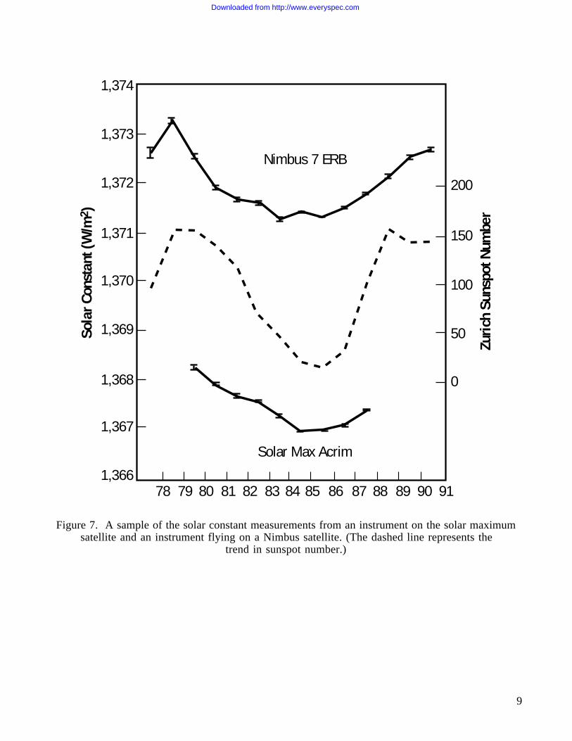
Spacecraft may receive radiant thermal energy from three sources: (1) incoming solar radi-ation (solar constant), (2) reflected solar energy (albedo), and (3) outgoing long-wave radiation(OLR) emitted by the Earth and atmosphere. If one considers the Earth and its atmosphere as awhole and averages over long time periods, the incoming solar energy and outgoing radiant energyare essentially in balance; the Earth/atmosphere is nearly in radiative equilibrium with the Sun.However, it is not in balance everywhere on the globe and there are important variations with localtime, geography, and atmospheric conditions. A space vehicle’s motion with respect to the Earthresults in its viewing only a “swath” across the full global thermal profile, so it sees these vari-ations as a function of time in accordance with the thermal time constants of its hardware systems(figs. 7 and 8).
Spacecraft Effects
Correct definition of the orbital thermal environment is an integral part of an effective space-craft thermal design. This thermal environment varies over orbits and over mission lifetime, whiletypical temperature control requirements for spacecraft components cover a predetermined range oftemperatures. Changes in temperature need to be minimized because they may lead to systemfatigue. An issue frequently encountered is the ability to provide adequate capability to cool sen-sitive electronic systems. Temperature fluctuations may fatigue delicate wires and solder joints,promoting system failures. Abrupt changes in the thermal environment may cause excessive freeze–thaw cycling of thermal control fluids. Too extreme an environment may require oversizing of radi-ators or possibly cause permanent radiator freezing. The thermal environment is also an importantfactor in considering lifetimes of cryogenic liquids or fuels.
New Developments
Advances in technology have led to stronger material bonding which has provided the spacecommunity with stronger flight materials at much reduced weight. These lightweight materials, how-ever, are more susceptible to changes in the thermal environment of space. This has led to a need fora much more accurate description of thermal environment variations. Previously, the design engineerhad only long-term, global mean thermal parameters to aid in the design process. Marshall SpaceFlight Center (MSFC) has completed analysis of data from the Earth radiation budget experiment(ERBE) which provides a significant advancement in the description of this near-Earth thermalenvironment. The new results provide thermal environment parameters which vary with orbitinclination and can be matched to a system’s thermal response time. The new thermal environmentdescription has already been incorporated in the space station program and other NASA programs.
Downloaded from http://www.everyspec.com
9
781,366
1,367
1,368
1,369
1,370
1,371
1,372 200
150
100
50
0
1,373
1,374
79 80 81 82 83
Sola
r Con
stan
t (W
/m2 )
Zuri
ch S
unsp
ot N
umbe
r84 85
Solar Max Acrim
Nimbus 7 ERB
86 87 88 89 90 91
Figure 7. A sample of the solar constant measurements from an instrument on the solar maximumsatellite and an instrument flying on a Nimbus satellite. (The dashed line represents the
trend in sunspot number.)
Downloaded from http://www.everyspec.com
10
Square Triangle Diamond Cross Plus
Extremes 1–99 3–97 5–95 50
Percentile Range Percentile Range Percentile Range Percentile Value
0.70
0.65
0.60
0.55
0.50
0.45
0.40
0.35
0.30
0.25
0.20
0.15
0.10
0.05
0.000.0 0.2 0.4 0.6 0.8 1.0
Time Interval (hours)
Tim
e Av
erag
ed A
lbed
o
1.2 1.4 1.6 1.8
Square Triangle Diamond Cross Plus
Extremes 1–99 3–97 5–95 50
Percentile Range Percentile Range Percentile Range Percentile Value
360.0
340.0
320.0
300.0
280.0
260.0
240.0
220.0
200.0
180.0
160.0
140.0
120.0
100.00.0 0.2 0.4 0.6 0.8 1.0
Time Interval (hours)
Tim
e Av
erag
e O
LR—
W/m
2
1.2 1.4 1.6 1.8
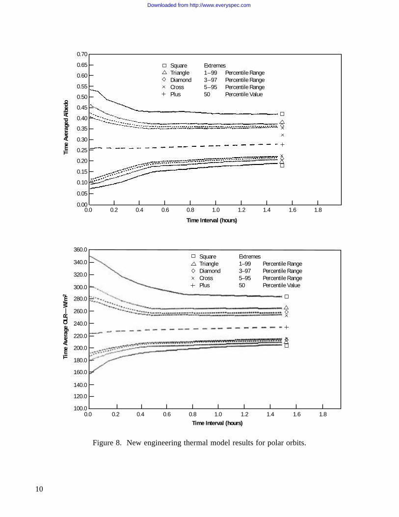
Figure 8. New engineering thermal model results for polar orbits.
Downloaded from http://www.everyspec.com
11
PLASMA
Environment Definition
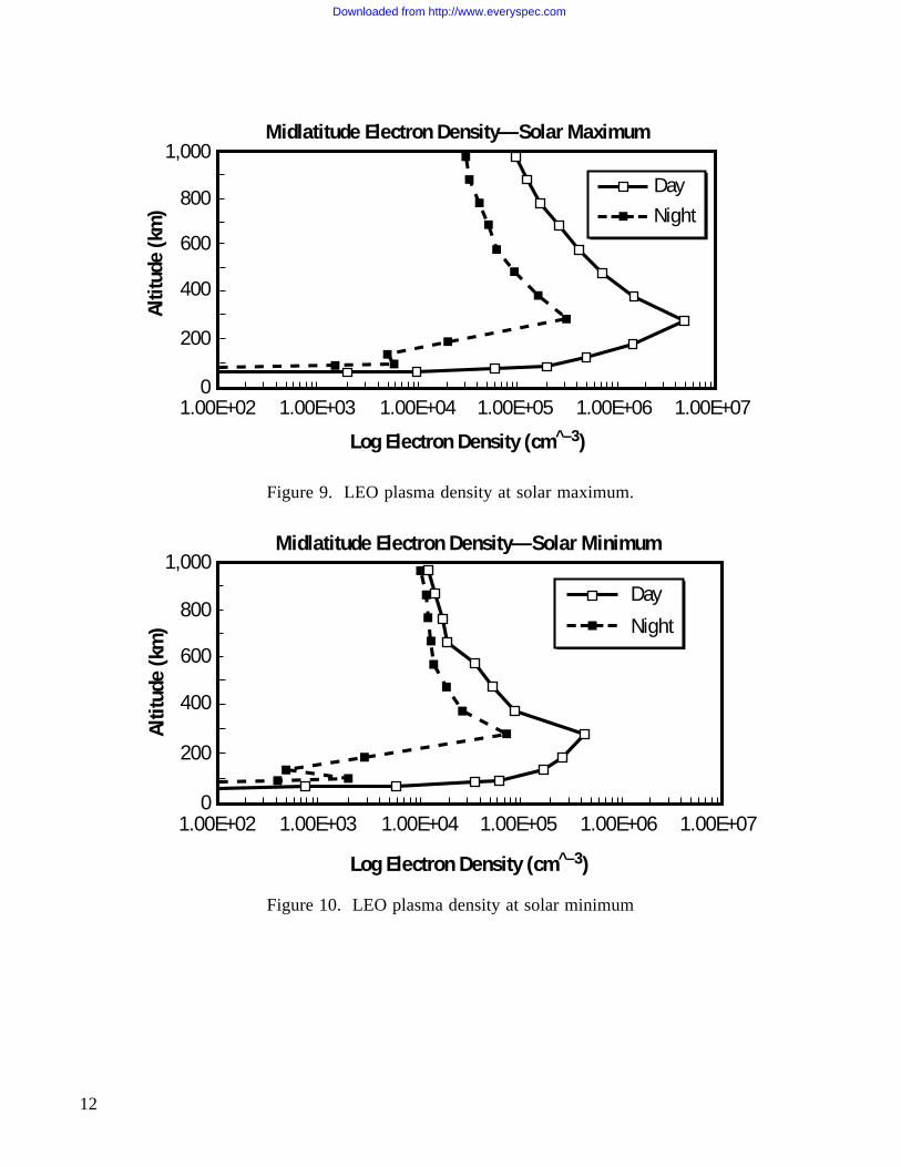
The major constituents of the Earth’s atmosphere remain virtually unchanged up to an alti-tude of 90 km, but above this level the relative amounts and types of gases are no longer constantwith altitude. Within this upper zone of thin air, shortwave solar radiation causes various photo-chemical effects on the gases. A photochemical effect is one in which the structure of a molecule ischanged when it absorbs radiant energy. One of the most common of these effects is the splitting ofdiatomic oxygen into atoms. Another common effect is that atoms will have electrons ejected fromtheir outer shells. These atoms are said to be ionized. A small part of the air in the upper atmo-sphere consists of these positively charged ions and free electrons which cause significant physicaleffects. The electron densities are approximately equal to the ion densities everywhere in the region.An ionized gas composed of equal numbers of positively and negatively charged particles is termed aplasma. Therefore, it is because of these characteristics that this electrically charged portion of theatmosphere is known as the ionosphere, and the gas within this layer is referred to as the iono-spheric plasma. The electron and ion densities vary dramatically with altitude, latitude, magneticfield strength, and solar activity (figs. 9 and 10).
Spacecraft Effects
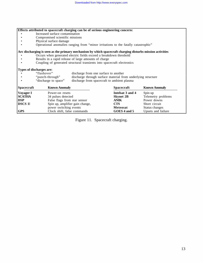
As a spacecraft flies through this ionized portion of the atmosphere, it may be subjected to anunequal flux of ions and electrons and may develop an induced charge. Plasma flux to the spacecraftsurface can charge the surface and disrupt the operation of electrically biased instruments (fig. 11).In LEO, vehicles travel through dense but low energy plasma. These spacecraft are negativelycharged because their orbital velocity is greater than the ion thermal velocity but slower than theelectron thermal velocity. Thus, electrons can impact all surfaces, while ions can impact only ramsurfaces. LEO spacecrafts have been known to charge to thousands of volts, however charging atgeosynchronous orbits is typically a greater concern. Biased surfaces, such as solar arrays, canaffect the floating potential. The magnitude of charge depends on the type of grounding configurationused. Spacecraft charging may cause: biasing of spacecraft instrument readings, arcing which maycause upsets to sensitive electronics, increased current collection, reattraction of contaminants, andion sputtering which may cause accelerated erosion of materials. High magnitude charging will causearcing and other electrical disturbances on spacecraft. Figure 12 shows some typical charging eventsthat have occurred on a polar orbiting spacecraft. A listing of some of the disturbances that havebeen noted by spacecraft charging is provided in figure 11.
New Developments
Spacecraft charging due to plasma interactions has been studied for some time for spacecraftat geosynchronous altitudes. Recently, however, there has been a new emphasis on studyingcharging effects on LEO spacecraft, especially those in polar orbits. A new computer model calledPOLAR has been developed to analyze spacecraft charging in low-Earth polar orbit. POLAR pro-vides detailed information on charging potentials anywhere on the spacecraft structure.
Downloaded from http://www.everyspec.com
12
1,000
800
600
400
200
01.00E+02 1.00E+03 1.00E+04
Log Electron Density (cm^–3)
Altit
ude
(km
)
1.00E+05 1.00E+06 1.00E+07
DayNight
Midlatitude Electron Density—Solar Maximum
Figure 9. LEO plasma density at solar maximum.
Altit
ude
(km
)
1,000
800
600
400
200
01.00E+02 1.00E+03 1.00E+04 1.00E+05 1.00E+06 1.00E+07
Midlatitude Electron Density—Solar Minimum
Log Electron Density (cm^–3)
Day
Night
Figure 10. LEO plasma density at solar minimum
Downloaded from http://www.everyspec.com
13
Effects attributed to spacecraft charging can be of serious engineering concern:• Increased surface contamination• Compromised scientific missions• Physical surface damage• Operational anomalies ranging from “minor irritations to the fatally catastrophic”
Arc discharging is seen as the primary mechanism by which spacecraft charging disturbs mission activities• Occurs when generated electric fields exceed a breakdown threshold• Results in a rapid release of large amounts of charge• Coupling of generated structural transients into spacecraft electronics
Types of discharges are:• “flashover” discharge from one surface to another• “punch-through” discharge through surface material from underlying structure• “discharge to space” discharge from spacecraft to ambient plasma
Spacecraft Known Anomaly Spacecraft Known Anomaly_________________________________ ________________________________ Voyager I Power-on resets Intelsat 3 and 4 Spin upSCATHA 34 pulses detected Skynet 2B Telemetry problemsDSP False flags from star sensor ANIK Power downsDSCS II Spin up, amplifier gain change, CTS Short circuit
power switching events Meteosat Status changesGPS Clock shift, false commands GOES 4 and 5 Upsets and failure
Figure 11. Spacecraft charging.
Downloaded from http://www.everyspec.com

14
109
108
107
106
105
102
103
300
200
100
49820 13:50:20
49840 49860 49880 49900 49920 u.t. 13:52:00 u.t.
Ion
Den
sity
(cm
–3)
Sate
llite
Pot
entia
l, –
Øsc
(vol
ts)
Inte
gral
Ele
ctro
n Fl
ux (E
lect
ron)
DMSP F7
E > 30 eV E > 14 keV
Figure 12. An example of the type of charging events encountered by the DMSP satellite F7 onNovember 26, 1983. DMSP 7 is a defense meteorological satellite flying in LEO/polar.
Downloaded from http://www.everyspec.com
15
METEOROID/ORBITAL DEBRIS
Environment Definition
The meteoroid population consists primarily of the remnants of comets. As a cometapproaches perihelion, the gravitational force and solar wind pressure on it are increased, resulting ina trail of particles in nearly the same orbit as the comet. When the Earth intersects a comet’s orbit,there is a meteor shower, and this occurs several times per year. The Earth also encounters manysporadic particles on a daily basis. These particles originate in the asteroid belt, and are themselvesthe smallest asteroids. Radiation pressure from the Sun causes a drag force on the smallest particlesin the asteroid belt. In time, these particles lose their orbital energy and spiral into the Sun.
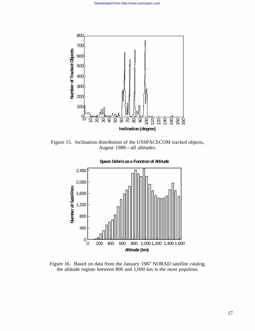
Since the beginning of human activity in space, there has been a growing amount of matter leftin orbit (figs. 13 through 16). In addition to operational payloads, there exist spent rocket stages,fragments of rockets and satellites, and other hardware and ejecta, many of which will remain in orbitfor many hundreds of years. Currently, the U.S. Air Force Space Command tracks over 7,000 largeobjects (>10 cm) in LEO, and the number of smaller objects is known to be in the tens of thousands.Since the orbital debris population continually grows, it will be an increasing concern for future spaceoperations.
Spacecraft Effects
Meteoroids and orbital debris pose a serious damage and decompression threat to spacevehicles. In the orbital velocity regime, collisions are referred to as hypervelocity impacts. Such animpact, for example, by a 90-gram particle, will impart over 1 MJ of energy to the vehicle. Thus,practically any spacecraft will suffer catastrophic damage or decompression if it receives a hyper-velocity impact from an object larger than a few grams. Collisions with smaller objects cause serioussurface erosion with subsequent effects on the surface thermal, electrical, and optical properties. Netrisk to a mission depends on the orbit duration, vehicle size and design, launch date (solar cyclephase), orbit altitude, and inclination. Protective shielding is often necessary to minimize the threatfrom the meteoroid/orbital debris environment. If a system cannot be shielded, operational con-straints or procedures may be imposed to reduce the threat of damage. The debris threat is highlydirectional, so risk can also be mitigated by careful arrangement of critical components.
New Developments
The orbital debris environment continues to increase because of continued activity in spaceand continued on-orbit fragmentation events. New data from radar measurements confirm the currentNASA models, in general, and will lead to improved descriptions of the altitude, inclination, andvelocity distributions of the debris environment.
Downloaded from http://www.everyspec.com

16
Fragmentation Debris (43%)
Active Pay- loads (5%)Launch
Debris (16%)
Rocket Body (15%)
Inactive Payloads
(21%)
5-21106
Figure 13. Sources of the catalogued debris population.
Figure 14. The state of the Earth debris environment is illustrated in this snapshot of all cataloguedobjects in July 1987.
Downloaded from http://www.everyspec.com
17
800
700
600
500
400
300
200
100
0
160
150
140
130
120
110
1009080706050403020100
Num
ber o
f Tra
cked
Obj
ects
Inclination (degree)
Figure 15. Inclination distribution of the USSPACECOM tracked objects,August 1988—all altitudes.
2,400
2,000
1,600
1,200
800
400
00 200 400 600 800 1,000 1,200 1,400 1,600
Altitude (km)
Num
ber o
f Sat
ellit
es
Space Debris as a Function of Altitude
5-21092
Figure 16. Based on data from the January 1987 NORAD satellite catalog,the altitude regime between 800 and 1,000 km is the most populous.
Downloaded from http://www.everyspec.com

18
SOLAR ENVIRONMENT
Environment Definition
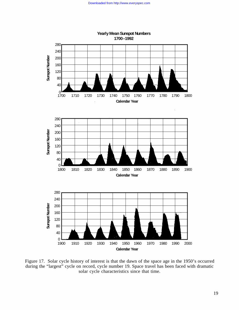
The Sun emits huge amounts of mass and energy; enough energy in 1 second to powerseveral million cars for over a billion years. This tremendous emission of energy has important con-sequences to spacecraft design, development, and operations. Over short periods of time and in cer-tain locations, solar intensity can fluctuate rapidly. It is thought that a major factor causing thesefluctuations is the distortion of the Sun’s large magnetic field due to its differential rotation. Two ofthe most common indicators of locally enhanced magnetic fields are sunspots and flares. Sunspotsare probably the most commonly known solar activity feature. The average sunspot number is knownto vary with a period of about 11 years (fig. 17). Each cycle is defined as beginning with solar mini-mum (the time of lowest sunspot number) and lasting until the following solar minimum. Forexample, cycle 22, which began in late 1986, reached solar maximum in 1991. A solar flare is a highlyconcentrated explosive release of energy within the solar atmosphere. The radiation from a solarflare extends from radio to x-ray frequencies. Solar flares are differentiated according to their totalenergy released. Ultimately, the total energy emitted is the deciding factor in the severity of a flare’seffects on the space environment.
Spacecraft Effects
The solar environment has a critical impact on most elements within the natural spaceenvironment. Variations in the solar environment impact thermospheric density levels, the overallthermal environment a spacecraft will experience, plasma density levels, meteoroids/orbital debrislevels, the severity of the ionizing radiation environment, and characteristics of the Earth’s magneticfield. The solar cycle also plays an important role in mission planning and mission operations activi-ties. For instance, when solar activity is high, ultraviolet and extreme ultraviolet radiation from theSun heats and expands the Earth’s upper atmosphere, increasing atmospheric drag and the orbitaldecay rate of spacecraft. Solar flares are a major contributor to the overall radiation environment andcan add to the dose of accumulated radiation levels and to single event phenomena which affectelectronic systems.
New Developments
The variability of the solar cycle has been effectively modeled using a proxy parameter, the10.7-cm solar radio flux (F10.7). The Environments Team at the Marshall Space Flight Centercurrently predicts and publishes a monthly solar activity memorandum which gives long-rangeestimates of both the F10.7 index and the geomagnetic activity index, Ap. Also, solar science ismaking progress toward predicting the sites for flare activity on the Sun in much the same way asmeteorologists have developed criteria for probable tornadic activity within the Earth’s atmosphere.As more is learned about the Sun’s behavior, more realistic modeling of the Sun is possible and moreaccurate predictions of the Sun’s future behavior can be made.
Downloaded from http://www.everyspec.com
19
280
240
200
160
120
80
40
01700 1710 1720 1730 1740 1750 1760 1770 1780 1790 1800
Calendar Year
Suns
pot N
umbe
r
280
240
200
160
120
80
40
01800 1810 1820 1830 1840 1850 1860 1870 1880 1890 1900
Calendar Year
Suns
pot N
umbe
r
280
240
200
160
120
80
40
01900 1910 1920 1930 1940 1950 1960 1970 1980 1990 2000
Calendar Year
Suns
pot N
umbe
r
Yearly Mean Sunspot Numbers 1700–1992
Figure 17. Solar cycle history of interest is that the dawn of the space age in the 1950’s occurredduring the “largest” cycle on record, cycle number 19. Space travel has been faced with dramatic
solar cycle characteristics since that time.
Downloaded from http://www.everyspec.com

20
IONIZING RADIATION
Environment Definition
The particles associated with ionizing radiation are categorized into three main groupsrelating to the source of the radiation: trapped radiation belt particles, cosmic rays, and solar flareparticles. Results from recent satellite studies suggest that the source of the trapped radiation belts(or Van Allen belts) particles seems to be from a variety of physical mechanisms: from the accel-eration of lower-energy particles by magnetic storm activity, from the trapping of decay products ofenergetic neutrons produced in the upper atmosphere by collisions of cosmic rays with atmosphericparticles, and from solar flares. Solar proton events are associated with solar flares. Cosmic raysoriginate from outside the solar system from other solar flares, nova/supernova explosions, orquasars.
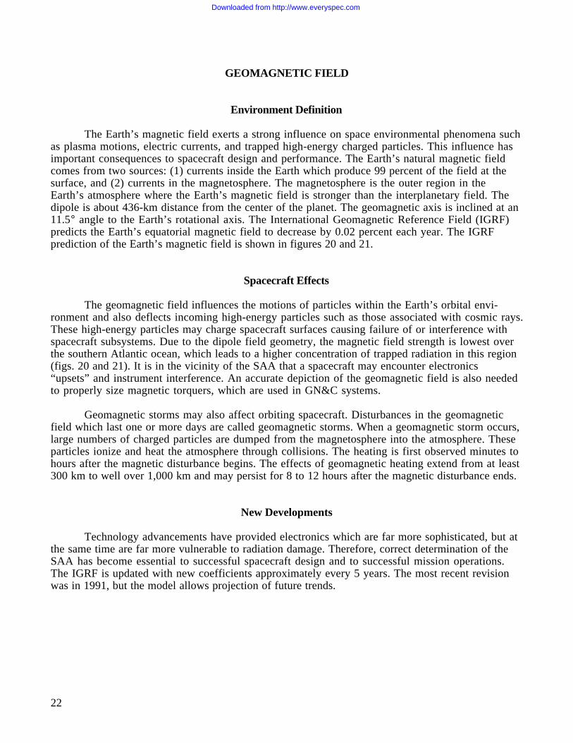
The Earth’s magnetic field concentrates large fluxes of high-energy, ionizing particlesincluding electrons, protons, and some heavier ions. The Earth’s magnetic field provides the mecha-nism which traps these charged particles within specific regions, called the Van Allen belts. Thebelts are characterized by a region of trapped protons and both an inner and an outer electron belt.The radiation belt particles spiral back and forth along the magnetic field lines (fig. 18). Because theEarth’s approximate dipolar field is displaced from the Earth’s center, the ionizing radiation beltsreach their lowest altitude off the eastern coast of South America. This means as particles travel intothis region they will reach lower altitudes, and particle densities will be anomalously high over thisregion. This area is termed the South Atlantic Anomaly (SAA). For the purpose of this document,the term “cosmic rays” applies to electrons, protons, and the nuclei of all elements from other thansolar origins. Satellites at low inclination and low altitude experience a significant amount of naturalshielding from cosmic rays due to the Earth’s magnetic field. A small percentage of solar flares areaccompanied by the ejection of significant numbers of protons. Solar proton events occur sporadically,but are most likely near solar maximum. Events may last hours or up to more than a week, but typi-cally the effects last 2 to 3 days. Solar protons add to the total dose and may also cause single-event effects in some cases (figs. 19a and 19b).
Spacecraft Effects
The high-energy particles comprising the radiation environment can travel through spacecraftmaterial and deposit kinetic energy. This process causes atomic displacement or leaves a stream ofcharged atoms in the incident particle’s wake. Spacecraft damage includes decreased power pro-duction by solar arrays, failure of sensitive electronics, increased background noise in sensors, andradiation exposure of the spacecraft crew. Modern electronics are becoming increasingly sensitive toionizing radiation.
New Developments
A new transient radiation belt containing large numbers of highly energetic electrons wasrecently encountered by the combined release and radiation effects satellite (CRRES). The solaranomalous and magnetospheric particle explorer (SAMPEX) satellite recently discovered a belt oftrapped anomalous ray particles that will effect LEO missions. Also, it is now realized that manyheavy ion cosmic rays are only partially ionized so that geomagnetic shielding of these particles isnot as effective as once thought.
Downloaded from http://www.everyspec.com
21
Flux Tube
Trajectory of Trapped Particle
Mirror Point
Magnetic Conjugate Point
North
Drift of Protons
Magnetic Field Line
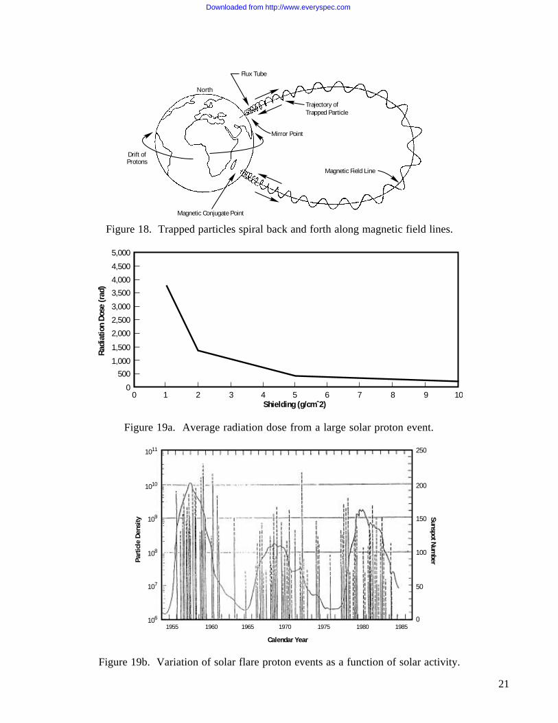
Figure 18. Trapped particles spiral back and forth along magnetic field lines.
0Shielding (g/cmˆ2)
Rad
iatio
n D
ose
(rad
)
0
500
1,000
1,500
2,000
2,500
3,000
4,000
5,000
3,500
4,500
1 2 3 4 5 6 7 8 9 10
Figure 19a. Average radiation dose from a large solar proton event.
1011
1010
109
108
107
106
1955 1960 1965 1970 1975 1980 19850
50
100
150
200
250
Calendar Year
Sunspot Num
berPart
icle
Den
sity
Figure 19b. Variation of solar flare proton events as a function of solar activity.
Downloaded from http://www.everyspec.com
22
GEOMAGNETIC FIELD
Environment Definition
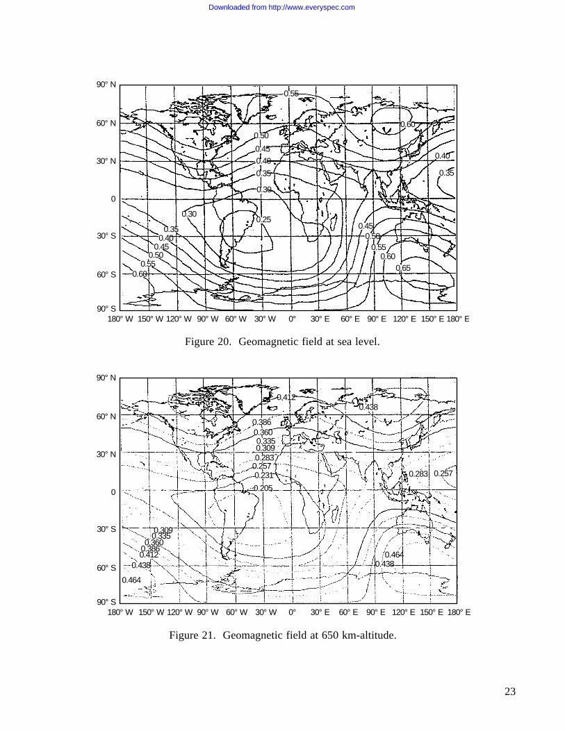
The Earth’s magnetic field exerts a strong influence on space environmental phenomena suchas plasma motions, electric currents, and trapped high-energy charged particles. This influence hasimportant consequences to spacecraft design and performance. The Earth’s natural magnetic fieldcomes from two sources: (1) currents inside the Earth which produce 99 percent of the field at thesurface, and (2) currents in the magnetosphere. The magnetosphere is the outer region in theEarth’s atmosphere where the Earth’s magnetic field is stronger than the interplanetary field. Thedipole is about 436-km distance from the center of the planet. The geomagnetic axis is inclined at an11.5° angle to the Earth’s rotational axis. The International Geomagnetic Reference Field (IGRF)predicts the Earth’s equatorial magnetic field to decrease by 0.02 percent each year. The IGRFprediction of the Earth’s magnetic field is shown in figures 20 and 21.
Spacecraft Effects
The geomagnetic field influences the motions of particles within the Earth’s orbital envi-ronment and also deflects incoming high-energy particles such as those associated with cosmic rays.These high-energy particles may charge spacecraft surfaces causing failure of or interference withspacecraft subsystems. Due to the dipole field geometry, the magnetic field strength is lowest overthe southern Atlantic ocean, which leads to a higher concentration of trapped radiation in this region(figs. 20 and 21). It is in the vicinity of the SAA that a spacecraft may encounter electronics“upsets” and instrument interference. An accurate depiction of the geomagnetic field is also neededto properly size magnetic torquers, which are used in GN&C systems.
Geomagnetic storms may also affect orbiting spacecraft. Disturbances in the geomagneticfield which last one or more days are called geomagnetic storms. When a geomagnetic storm occurs,large numbers of charged particles are dumped from the magnetosphere into the atmosphere. Theseparticles ionize and heat the atmosphere through collisions. The heating is first observed minutes tohours after the magnetic disturbance begins. The effects of geomagnetic heating extend from at least300 km to well over 1,000 km and may persist for 8 to 12 hours after the magnetic disturbance ends.
New Developments
Technology advancements have provided electronics which are far more sophisticated, but atthe same time are far more vulnerable to radiation damage. Therefore, correct determination of theSAA has become essential to successful spacecraft design and to successful mission operations.The IGRF is updated with new coefficients approximately every 5 years. The most recent revisionwas in 1991, but the model allows projection of future trends.
Downloaded from http://www.everyspec.com
23
180° W
90° N
60° N
30° N
0
30° S
60° S
90° S150° W 120° W 90° W 60° W 30° W 0° 30° E 60° E 90° E 120° E 150° E 180° E
0.55
0.60
0.55
0.50
0.50
0.500.55
0.60
0.600.65
0.45
0.45
0.45
0.40
0.40
0.40
0.35
0.35
0.35
0.30
0.300.25
Figure 20. Geomagnetic field at sea level.
180° W
90° N
60° N
30° N
0
30° S
60° S
90° S150° W 120° W 90° W 60° W 30° W 0° 30° E 60° E 90° E 120° E 150° E 180° E
0.412
0.4120.438
0.438
0.464
0.3860.360
0.3600.386
0.335
0.335
0.309
0.309
0.283
0.283 0.257
0.4640.438
0.2570.231
0.205
Figure 21. Geomagnetic field at 650 km-altitude.
Downloaded from http://www.everyspec.com

24
GRAVITATIONAL FIELD
Environment Definition
Since the advent of Earth satellites, there has been a considerable advancement in the accu-rate determination of the Earth’s gravitational field. The current knowledge regarding the Earth’sgravitational field has advanced far beyond the normal operational requirements of most space mis-sions. Adequate accuracy for determining most spacecraft design values of gravitational interactionsis obtained with the central inverse square field:
F = –µEm
r 2 r .
The above central force model accurately represents the gravitational field to approximately0.1 percent. If this accuracy is insufficient for particular program needs, a more detailed model of thegravitational field can be used that accounts for the nonuniform mass distribution within the Earth.This model gives the gravitational potential, V, to an accuracy of approximately a few parts in a mil-lion. The gravitational acceleration is expressed in terms of the negative gradient of the potential.The potential is then expressed using harmonic expansion:
F = mg = m(–∇V ) .
Spacecraft Effects
Accurate predictions of the Earth’s gravitational field are a critical part of mission planningand design for any spacecraft. The Earth’s gravitational field will affect spacecraft orbits and trajec-tories. Gravity models are used to estimate the gravitational field strength for use in designing theGN&C/pointing subsystem, and designing the telemetry, tracking, and communications. Theavailable gravitational models have sufficient accuracy for estimating the gravitational field strengthfor spacecraft planning and design.
New Developments
Gravitational models of the Earth are continually being updated and upgraded. Currently,gravitational models are available for varying degrees of accuracy. For operational applications andother situations where computer resources are a premium, “best fit” approximations to the highestaccuracy model may be utilized which minimize the computational requirements yet retain therequired accuracy for the specific application.
Downloaded from http://www.everyspec.com

25
CONCLUSION
For optimum efficiency and effectiveness, it is important that the need for definition of theflight environment be recognized very early in the design and development cycle of a spacecraft.From past experience, the earlier the environments specialists become involved in the design pro-cess, the less potential for negative environmental impacts on the program through redesign, opera-tional work-arounds, etc. The key steps in describing the natural space environment for a particularprogram include the following:
• Definition of the flight environment is the first critical step. Since the environment dependsstrongly on orbit and phase of the solar cycle, environment effects should be reviewed prior tofinal orbit selection.
• Not all space environments will have a critical impact on a particular mission. It is the role of theenvironments specialists to find all the environmental limiting factors for each program and tooffer design or operational solutions to the program where possible. This typically requires aclose working relationship between the environments specialists, members of the design teams,and program management. Typically, once the limiting factors are established, trade studies areusually required to establish the appropriate environmental definition.
• After definition of the space environment is established including results from trade studies, thenext important step is to establish a coordinated set of natural space environment requirementsfor use in design and development. These requirements are derived directly from the definitionphase and again, typically are derived after much interaction among the design developmentengineering staff, program management, and environments specialists.
• Typically, the space environment definition and requirements are documented in a separate pro-gram document or are incorporated into design and performance specifications.
• The environments specialist then helps insure that the environment specifications are understoodand correctly interpreted throughout the design, development, and operational phases of the pro-gram.
This primer has provided an overview of the natural space environments and their effect onspacecraft design, development, and operations. It is hoped that a better understanding of the spaceenvironment and its effect on spacecraft will enable program management to more effectivelyminimize program risks and costs, optimize design quality, and successfully achieve missionobjectives. If you have further questions or comments, contact the MSFC Systems Analysis andIntegration Laboratory’s Electromagnetics and Environments Branch, Steven D. Pearson at 205–544–2350.
Downloaded from http://www.everyspec.com


