The Metal Processing Module User’s Guide - doc.comsol.com

Metal Processing ModuleUser’s Guide

C o n t a c t I n f o r m a t i o n

Visit the Contact COMSOL page at www.comsol.com/contact to submit general inquiries, contact Technical Support, or search for an address and phone number. You can also visit the Worldwide Sales Offices page at www.comsol.com/contact/offices for address and contact information.

If you need to contact Support, an online request form is located at the COMSOL Access page at www.comsol.com/support/case. Other useful links include:

• Support Center: www.comsol.com/support

• Product Download: www.comsol.com/product-download

• Product Updates: www.comsol.com/support/updates

• COMSOL Blog: www.comsol.com/blogs

• Discussion Forum: www.comsol.com/community

• Events: www.comsol.com/events

• COMSOL Video Gallery: www.comsol.com/video

• Support Knowledge Base: www.comsol.com/support/knowledgebase

Part number: CM025001

M e t a l P r o c e s s i n g M o d u l e U s e r ’ s G u i d e© 1998–2020 COMSOL

Protected by patents listed on www.comsol.com/patents, and U.S. Patents 7,519,518; 7,596,474; 7,623,991; 8,457,932; 9,098,106; 9,146,652; 9,323,503; 9,372,673; 9,454,625; 10,019,544; 10,650,177; and 10,776,541. Patents pending.

This Documentation and the Programs described herein are furnished under the COMSOL Software License Agreement (www.comsol.com/comsol-license-agreement) and may be used or copied only under the terms of the license agreement.

COMSOL, the COMSOL logo, COMSOL Multiphysics, COMSOL Desktop, COMSOL Compiler, COMSOL Server, and LiveLink are either registered trademarks or trademarks of COMSOL AB. All other trademarks are the property of their respective owners, and COMSOL AB and its subsidiaries and products are not affiliated with, endorsed by, sponsored by, or supported by those trademark owners. For a list of such trademark owners, see www.comsol.com/trademarks.

Version: COMSOL 5.6

www.comsol.com/patents/

https://www.comsol.com/comsol-license-agreement/

http://www.comsol.com/contact/

http://www.comsol.com/contact/offices/

http://www.comsol.com/support/case/

http://www.comsol.com/support/

http://www.comsol.com/product-download/

http://www.comsol.com/support/updates/

https://www.comsol.com/trademarks/

http://www.comsol.com/blogs/

http://www.comsol.com/community/

http://www.comsol.com/events/

http://www.comsol.com/video/

http://www.comsol.com/support/knowledgebase/

C o n t e n t s

C h a p t e r 1 : I n t r o d u c t i o n

About the Metal Processing Module 8

What Can the Metal Processing Module Do? . . . . . . . . . . . . 8

Where Do I Access the Documentation and Application Libraries? . . . . 9

Overview of the User’s Guide 12

C h a p t e r 2 : M e t a l P r o c e s s i n g M o d e l i n g

Selecting Physics Interfaces 16

Metal Phase Transformation . . . . . . . . . . . . . . . . . . 16

Austenite Decomposition . . . . . . . . . . . . . . . . . . . 16

Carburization . . . . . . . . . . . . . . . . . . . . . . . . 17

Study Types 18

Modeling Phase Transformations 19

Metallurgical Phases . . . . . . . . . . . . . . . . . . . . . . 19

Phase Transformations . . . . . . . . . . . . . . . . . . . . 19

Calibration of Phase Transformation Models . . . . . . . . . . . . 21

Defining Multiphysics Models 25

Heat Transfer with Phase Transformations . . . . . . . . . . . . . 25

Steel Quenching . . . . . . . . . . . . . . . . . . . . . . . 26

Phase Transformation Latent Heat . . . . . . . . . . . . . . . . 27

Phase Transformation Strain . . . . . . . . . . . . . . . . . . 28

Selecting Discretizations 29

Phase Transformation Modeling . . . . . . . . . . . . . . . . . 29

Carburization Modeling . . . . . . . . . . . . . . . . . . . . 29

C O N T E N T S | 3

4 | C O N T E N T S

Using Effective Material Properties 30

Importing Material Properties 31

Modeling Carburization 32

Defining a Carburization Environment . . . . . . . . . . . . . . . 32

Modeling Carbon Diffusion . . . . . . . . . . . . . . . . . . . 32

Boundary Conditions . . . . . . . . . . . . . . . . . . . . . 33

References 34

C h a p t e r 3 : M e t a l P r o c e s s i n g T h e o r y

Metal Phase Transformation Theory 36

Metallurgical Phase Transformations 37

Definitions . . . . . . . . . . . . . . . . . . . . . . . . . 37

Phase Transformation Models . . . . . . . . . . . . . . . . . . 38

Compound Material Properties 42

Heat Transfer Properties . . . . . . . . . . . . . . . . . . . . 42

Mechanical Properties . . . . . . . . . . . . . . . . . . . . . 43

Phase Transformation Strains 46

Thermal Expansion . . . . . . . . . . . . . . . . . . . . . . 46

Transformation-Induced Plasticity . . . . . . . . . . . . . . . . 47

Total Strain Contribution . . . . . . . . . . . . . . . . . . . 48

Phase Transformation Latent Heat 49

Carburization 50

Carbon Potential Model . . . . . . . . . . . . . . . . . . . . 50

Boundary Conditions . . . . . . . . . . . . . . . . . . . . . 51

References 53

C h a p t e r 4 : M e t a l P h a s e T r a n s f o r m a t i o n

The Metal Phase Transformation Interface 56

Metallurgical Phase . . . . . . . . . . . . . . . . . . . . . . 58

Phase Transformation . . . . . . . . . . . . . . . . . . . . . 61

Transformation Condition . . . . . . . . . . . . . . . . . . . 62

C h a p t e r 5 : A u s t e n i t e D e c o m p o s i t i o n

The Austenite Decomposition Interface 64

C h a p t e r 6 : C a r b u r i z a t i o n

The Carburization Interface 68

Carburization . . . . . . . . . . . . . . . . . . . . . . . . 68

Carbon Flux. . . . . . . . . . . . . . . . . . . . . . . . . 69

Zero Carbon Flux . . . . . . . . . . . . . . . . . . . . . . 69

Carbon Concentration . . . . . . . . . . . . . . . . . . . . 69

Initial Values . . . . . . . . . . . . . . . . . . . . . . . . 69

C h a p t e r 7 : M u l t i p h y s i c s I n t e r f a c e s a n d C o u p l i n g s

Heat Transfer with Phase Transformations 72

On the Constituent Physics Interfaces . . . . . . . . . . . . . . . 72

Steel Quenching 73

On the Constituent Physics Interfaces . . . . . . . . . . . . . . . 73

C O N T E N T S | 5

6 | C O N T E N T S

Phase Transformation Latent Heat Multiphysics Coupling 74

Phase Transformation Strain Multiphysics Coupling 76

1

I n t r o d u c t i o n

This guide describes the Metal Processing Module, an optional add-on package for the COMSOL Multiphysics® simulation software. The module is designed to perform transient analyses of processes involving metallurgical (solid-solid) phase transformations in, mainly, steels. This chapter introduces you to the capabilities of the Metal Processing Module and includes a summary of the physics interfaces and where you can find the documentation.

In this chapter:

• About the Metal Processing Module

7

8 | C H A P T E R

Abou t t h e Me t a l P r o c e s s i n g Modu l e

In this section:

• What Can the Metal Processing Module Do?

• Where Do I Access the Documentation and Application Libraries?

What Can the Metal Processing Module Do?

The Metal Processing Module can be used to model different physical phenomena related to heat treatment of metals. Using this module, you can study how metallurgical phase transformations change the microstructure of a metallic material during a heating or cooling process. One example is the quenching of automotive steel transmission components, where the resulting microstructure is tailored to meet specific demands on strength and durability. Other examples include the study of phase transformations that occur during additive manufacturing of metal components and phase transformations in the heat-affected zone during welding.

There are five physics interfaces in the Metal Processing Module:

• The Metal Phase Transformation interface for studying diffusive and displacive metallurgical phase transformations in materials like steels.

• The Austenite Decomposition interface for specifically studying the cooling of steel from an austenitic state.

• The Carburization interface for studying the heat treatment process of carburization.

• The Heat Transfer with Phase Transformations interface for modeling thermal processes involving metallurgical phase transformations.

• The Steel Quenching interface for modeling coupled thermal and mechanical processes involving metallurgical phase transformations.

Throughout the Metal Processing User’s Guide, the Metal Phase Transformation and Austenite Decomposition physics interfaces are collectively referred to as phase transformation physics interfaces.

The physics interfaces in the Metal Processing Module can be added from the Model Wizard’s Select Physics page under Heat Transfer>Metal Processing. The physics interfaces can also be added by right-clicking a Component node and selecting Add

Physics.

1 : I N T R O D U C T I O N

Where Do I Access the Documentation and Application Libraries?

A C C E S S I N G T H E M E T A L P R O C E S S I N G M O D U L E D O C U M E N T A T I O N

The Metal Processing Module feature information, including theory and modeling details, is included in the Metal Processing Module User’s Guide.

When you install COMSOL Multiphysics, the documentation sets are installed in several locations, both on your computer and most easily accessible while you are working in COMSOL Multiphysics. The next section details where to access it.

A C C E S S I N G C O M S O L D O C U M E N T A T I O N A N D A P P L I C A T I O N L I B R A R I E S

A number of internet resources have more information about COMSOL, including licensing and technical information. The electronic documentation, topic-based (or context-based) help, and the application libraries are all accessed through the COMSOL Desktop.

T H E D O C U M E N T A T I O N A N D O N L I N E H E L P

The COMSOL Multiphysics Reference Manual describes the core physics interfaces and functionality included with the COMSOL Multiphysics license. This book also has instructions about how to use COMSOL Multiphysics and how to access the electronic Documentation and Help content.

Opening Topic-Based HelpThe Help window is useful as it is connected to the features in the COMSOL Desktop. To learn more about a node in the Model Builder, or a window on the Desktop, click to highlight a node or window, then press F1 to open the Help window, which then displays information about that feature (or click a node in the Model Builder followed by the Help button ( ). This is called topic-based (or context) help.

If you are reading the documentation as a PDF file on your computer, the blue links do not work to open an application or content referenced in a different guide. However, if you are using the Help system in COMSOL Multiphysics, these links work to open other modules, application examples, and documentation sets.

A B O U T T H E M E T A L P R O C E S S I N G M O D U L E | 9

10 | C H A P T E R

Opening the Documentation Window

T H E A P P L I C A T I O N L I B R A R I E S W I N D O W

Each model or application includes documentation with the theoretical background and step-by-step instructions to create a model or application. The models and applications are available in COMSOL Multiphysics as MPH files that you can open for further investigation. You can use the step-by-step instructions and the actual models as templates for your own modeling. In most models, SI units are used to describe the relevant properties, parameters, and dimensions, but other unit systems are available.

Once the Application Libraries window is opened, you can search by name or browse under a module folder name. Click to view a summary of the model or application and its properties, including options to open it or its associated PDF document.

Opening the Application Libraries WindowTo open the Application Libraries window ( ):

C O N T A C T I N G C O M S O L B Y E M A I L

For general product information, contact COMSOL at [email protected].

C O M S O L A C C E S S A N D T E C H N I C A L S U P P O R T

To receive technical support from COMSOL for the COMSOL products, please contact your local COMSOL representative or send your questions to [email protected]. An automatic notification and a case number are sent to you by email. You can also access technical support, software updates, license information, and other resources by registering for a COMSOL Access account.


C O M S O L O N L I N E R E S O U R C E S

COMSOL website www.comsol.com

Contact COMSOL www.comsol.com/contact

COMSOL Access www.comsol.com/access

Support Center www.comsol.com/support

Product Download www.comsol.com/product-download

Product Updates www.comsol.com/support/updates

COMSOL Blog www.comsol.com/blogs

Discussion Forum www.comsol.com/community

Events www.comsol.com/events

COMSOL Application Gallery www.comsol.com/models

COMSOL Video Gallery www.comsol.com/video

Support Knowledge Base www.comsol.com/support/knowledgebase

A B O U T T H E M E T A L P R O C E S S I N G M O D U L E | 11

https://www.comsol.com

https://www.comsol.com/contact/

https://www.comsol.com/access

https://www.comsol.com/support/

https://www.comsol.com/product-download/

https://www.comsol.com/support/updates

https://www.comsol.com/blogs/

https://www.comsol.com/community

https://www.comsol.com/events/

http://www.comsol.com/models/

http://www.comsol.com/video/

http://www.comsol.com/support/knowledgebase/

12 | C H A P T E R

Ove r v i ew o f t h e U s e r ’ s Gu i d eT A B L E O F C O N T E N T S A N D I N D E X

To help you navigate this guide, see the Contents and Index sections.

M O D E L I N G W I T H T H E M E T A L P R O C E S S I N G M O D U L E

The Metal Processing Modeling chapter discusses how to model different problems involving phase transformations. The content covers the topics Selecting Physics Interfaces, Study Types, Modeling Phase Transformations, Defining Multiphysics Models, Selecting Discretizations, and Using Effective Material Properties.

M E T A L P R O C E S S I N G T H E O R Y

The Metal Processing Theory chapters outlines the theory for the interfaces present in the Metal Processing Module. The chapter covers the topics Metallurgical Phase Transformations, Compound Material Properties, Phase Transformation Strains, Phase Transformation Latent Heat, and Carburization.

T H E M E T A L P H A S E T R A N S F O R M A T I O N I N T E R F A C E

The Metal Phase Transformation chapter describes the Metal Phase Transformation interface and its feature nodes.

T H E A U S T E N I T E D E C O M P O S I T I O N I N T E R F A C E

The Austenite Decomposition chapter describes the Austenite Decomposition interface and how it is based on the Metal Phase Transformation Interface.

T H E C A R B U R I Z A T I O N I N T E R F A C E

The Carburization chapter describes the Carburization interface and its feature nodes.

M U L T I P H Y S I C S I N T E R F A C E S A N D C O U P L I N G S

The Multiphysics Interfaces and Couplings chapter describes two multiphysics interfaces found under the Metal Processing branch when adding a physics interface:

• The Heat Transfer with Phase Transformations interface combines a Metal Phase Transformation interface with a Heat Transfer in Solids interface. The coupling of the interfaces appears on a domain level, where produced latent heat from the (temperature-dependent) phase transformations gives rise to a heat source in the heat equation. Optionally, phase-composition-dependent thermal material properties can be used in the heat transfer analysis.


• The Steel Quenching Interface combines an Austenite Decomposition interface with a Heat Transfer in Solids interface and a Solid Mechanics interface. There are two domain-level multiphysics couplings: In the first coupling, produced latent heat from the (temperature-dependent) phase transformations gives rise to a heat source in the heat equation. In the second coupling, phase transformation strains that result from thermal expansion or transformation-induced plasticity (TRIP) are transferred to the Solid Mechanics interface as inelastic strain contributions for the computation of stresses. In the case of plasticity, the coupling also involves equivalent plastic strains and hardening functions. Optionally, phase-composition-dependent thermal and mechanical properties can be used in the heat transfer and solid mechanics analyses.

• The Phase Transformation Latent Heat multiphysics coupling adds the latent heat that is produced during phase transformations, as a heat source term, to the heat equation in a Heat Transfer interface.

• The Phase Transformation multiphysics coupling adds the transformation strains that are produced during phase transformations, as an inelastic strain contribution, to the equation for stress in a Solid Mechanics interface. The coupling also transfers stresses and the equivalent plastic strain from a Solid Mechanics interface to the coupled phase transformation interface.

O V E R V I E W O F T H E U S E R ’ S G U I D E | 13

14 | C H A P T E R

2

M e t a l P r o c e s s i n g M o d e l i n g

The goal of this chapter is to show you how to model different problems involving phase transformations in steels and how to include various physical phenomena that may be relevant in specific situations.

In this chapter:

• Selecting Physics Interfaces

• Study Types

• Modeling Phase Transformations

• Defining Multiphysics Models

• Selecting Discretizations

• Using Effective Material Properties

• Importing Material Properties

• Modeling Carburization

15

16 | C H A P T E R

S e l e c t i n g Ph y s i c s I n t e r f a c e s

The Metal Processing Module contains three basic physics interfaces and two multiphysics interfaces. The three basic physics interfaces are:

• Metal Phase Transformation — For modeling general metallurgical phase transformations

• Austenite Decomposition — For modeling the specific case of austenite decomposing into a combination of destination phases, on cooling

• Carburization — For modeling carburization; the process by which carbon from a surrounding carbon rich environment diffuses into a component.

Metal Phase Transformation

The Metal Phase Transformation interface provides a basic way to model phase transformations in metals. Three common models for phase transformations in steels are provided. The Leblond–Devaux and Johnson–Mehl–Avrami–Kolmogorov (JMAK) models are used to model time-dependent (diffusion-controlled) phase transformations, such as the transformation of austenite into pearlite during steel hardening. In contrast, the Koistinen–Marburger model is used to model the transformation of austenite into martensite, where the amount of undercooling below the so-called martensite start temperature controls the formation of martensite. In addition to these three types of phase transformations, you can define your own phase transformation models and let them coexist with other active phase transformations in your analysis. You can use an arbitrary number of phase transformations in a model. The Metal Phase Transformation interface lets you generate a compound material whose properties are phase composition dependent. This material can be used by other physics interfaces, such as Solid Mechanics and Heat Transfer in Solids.

Austenite Decomposition

The Austenite Decomposition interface is a specialized interface that considers hardening of steel from an austenitic state. During hardening of steels, the material is


• Metallurgical Phase Transformations

2 : M E T A L P R O C E S S I N G M O D E L I N G

heated above the austenitizing temperature. It is then cooled, and depending on the rate of cooling, a combination of destination phases such as ferrite, pearlite, bainite, and martensite can form. The Austenite Decomposition interface automatically creates corresponding phase nodes and phase transformation nodes. You can also define an arbitrary number of additional phases and phase transformations. Optionally, you can define your own phase transformation models and let them coexist with other active phase transformations in the analysis. The Austenite Decomposition interface lets you generate a compound material whose properties are phase-composition dependent. This material can be used by other physics interfaces, such as Solid Mechanics and Heat Transfer in Solids.

Carburization

The Carburization interface provides a way to model the heat treatment process of carburization. The process involves placing a component in a carbon rich environment, at an elevated temperature. Over time, carbon is transferred into the surface of the component, and then progresses to the interior via diffusion. You can specify the carbon potential (the carbon concentration of the surrounding environment) as a function of time, to emulate a particular process. Or, you can use a simplified boost-diffuse carburization cycle that is provided by the interface. You can model the mass transfer of carbon into the surface of the component in different ways. You can prescribe the carbon concentration at the surface, or use a convective, thermally activated carbon mass transfer. Additionally, you can model selective carburization by prescribing zero carbon flux in certain regions of the component surface.



S E L E C T I N G P H Y S I C S I N T E R F A C E S | 17

18 | C H A P T E R

S t u d y T yp e s

Metallurgical Phase transformations are inherently time dependent. Phase transformations are defined by a set of ordinary differential equations in time. The Carburization interface solves the time-dependent diffusion of carbon in a component. The only supported study type for the Metal Processing physics interfaces is therefore Time Dependent.

In the COMSOL Multiphysics Reference Manual:

• Time-Dependent Solver

• Studies and Solvers


Mode l i n g Pha s e T r a n s f o rma t i o n s

This section describes how to model metallurgical solid-solid phase transformations. When you simulate processes such as hardening of steel, these phase transformations are fundamental because they ultimately determine the final properties of the material. In the Metal Phase Transformation and Austenite Decomposition interfaces, each phase transformation is defined by a certain evolution equation that defines the time rate of change of the algebraic proportion of a destination phase at the expense of a source phase. In the following, the two modeling concepts of phases and phase transformations are discussed.

Metallurgical Phases

When you model phase transformations in a material, each transformation defines how a source phase transforms into a destination phase as a function of time. When you create a metallurgical phase node, you have to define its initial phase fraction. This is the value from which the phase fraction evolves during the analysis.

You have the option, at the physics interface level, to compute effective thermal and mechanical properties for the compound material. If you have opted to do this, you also need to define the corresponding properties of each phase. At each phase node, you can choose to create a component-level phase material. This material can be populated with properties that define the behavior of the phase. As an alternative, you can use imported material properties. This is described in Importing Material Properties.

The phase material properties are averaged (phase-fraction averaged) into effective material properties of a compound material that can be used in other physics interfaces. This is described in Using Effective Material Properties.

Phase Transformations

When you have created a phase transformation node, you have to choose a source phase and a destination phase. These are the two phases that are involved in the phase transformation. You then have to define a phase transformation model which defines the underlying type of phase transformation. The phase transformation models are described below.

M O D E L I N G P H A S E T R A N S F O R M A T I O N S | 19

20 | C H A P T E R

T H E L E B L O N D – D E V A U X M O D E L

Phase transformations in steels are based on diffusion of carbon, and the Leblond–Devaux phase transformation model is suitable to model this. You can choose between two formulations for the model — General coefficients or Time and equilibrium. Both these formulations require generally temperature-dependent functions that determine the characteristics of the phase transformation. The functions will be different for different phase transformations.

T H E J O H N S O N – M E H L – A V R A M I – K O L M O G O R O V ( J M A K ) M O D E L

This model can be viewed as a generalization of the Time and equilibrium form of the Leblond–Devaux model. In addition to the generally time-dependent functions describing the equilibrium phase fraction and the time constant, a time-dependent exponent is used. The exponent is called the Avrami exponent, and it alters the characteristic of the phase transformation.

T H E K O I S T I N E N – M A R B U R G E R M O D E L

This phase transformation model is suitable to model the displacive martensitic transformation in steel, on rapid cooling. The Martensite start temperature Ms can be experimentally obtained from dilatometry experiments. If the integrated form of the phase transformation model is used (Equation 3-7), a value for the Koistinen–

Marburger coefficient β can be correlated to the temperature at which the martensitic transformation is considered complete (see, for example, Ref. 8). The Martensite start

temperature smoothing is used to numerically smoothen the otherwise sudden onset of the martensitic transformation.

The Leblond–Devaux Model

The Johnson–Mehl–Avrami–Kolmogorov (JMAK) Model

The Koistinen–Marburger Model


Calibration of Phase Transformation Models

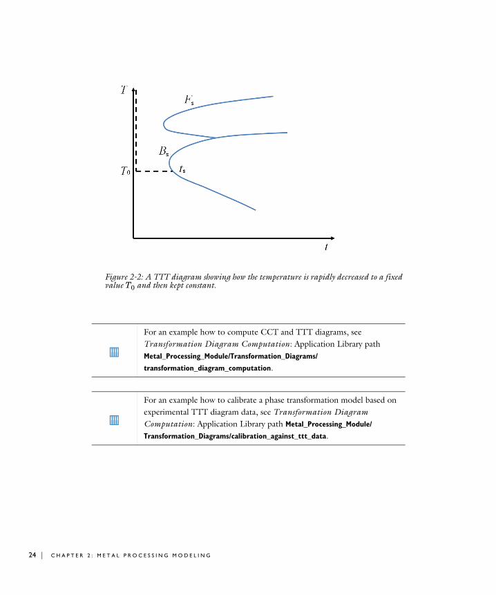
During a thermal transient, a material point may undergo varying rates of cooling and heating. During this transient, several phase transformations can be active at the same time. This suggests that it is difficult to calibrate phase transformation models individually, as they tend to affect one another. It is common in practice to present the complicated nature of the austenite decomposition as continuous cooling transformation (CCT) or time-temperature transformation (TTT) diagrams; see Figure 2-1 and Figure 2-2 for schematic examples. Both diagrams show the start temperatures for the formation of a small fraction of different phases (Fs for the start temperature of ferrite, and so on). The fraction can be chosen arbitrarily but is often 0.1% or 1%. The difference between the two diagram types, as their names imply, is the following:

• A CCT diagram is constructed by performing experiments where a small specimen is cooled at a specified, constant, temperature rate.

• A TTT diagram is constructed by performing experiments where a small specimen is rapidly cooled to a temperature T0 that is subsequently kept constant.

One method to measure the actual start temperatures required to draw each diagram is to use dilatometry experiments. Metallurgical phase transformations are accompanied by a change in volume, owing to the density difference between phases. In a dilatometer, a specimen is cooled (or heated), and its length is monitored. The specimen length will change according to basic thermal expansion, but phase transformations will induce additional length changes that can be measured.

In a real quenching situation, it is clear that material points do not experience either of the two extremes represented by the CCT and TTT diagrams (constant temperature rate versus constant temperature). Nevertheless, because experimentally obtained CCT and TTT diagrams are very common in the heat treatment community, phase transformation models must in practice be calibrated using them.

It is here useful to examine one form for the Leblond–Devaux model:

For an example how to model phase transformations, see Phase Transformations in a Round Bar: Application Library path Metal_Processing_Module/Tutorial_Examples/

phase_transformations_in_a_round_bar.


22 | C H A P T E R

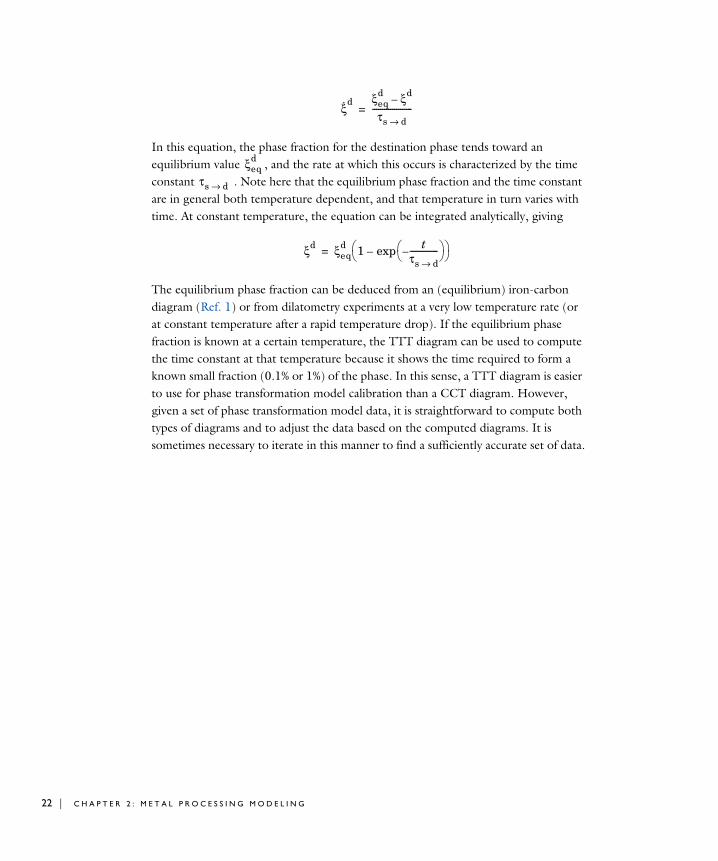
In this equation, the phase fraction for the destination phase tends toward an equilibrium value , and the rate at which this occurs is characterized by the time constant . Note here that the equilibrium phase fraction and the time constant are in general both temperature dependent, and that temperature in turn varies with time. At constant temperature, the equation can be integrated analytically, giving

The equilibrium phase fraction can be deduced from an (equilibrium) iron-carbon diagram (Ref. 1) or from dilatometry experiments at a very low temperature rate (or at constant temperature after a rapid temperature drop). If the equilibrium phase fraction is known at a certain temperature, the TTT diagram can be used to compute the time constant at that temperature because it shows the time required to form a known small fraction (0.1% or 1%) of the phase. In this sense, a TTT diagram is easier to use for phase transformation model calibration than a CCT diagram. However, given a set of phase transformation model data, it is straightforward to compute both types of diagrams and to adjust the data based on the computed diagrams. It is sometimes necessary to iterate in this manner to find a sufficiently accurate set of data.

ξ·d ξeq

d ξd–

τs d→--------------------=

ξeqd

τs d→

ξd ξeqd 1 t

τs d→--------------–

exp– =


Figure 2-1: A CCT diagram showing how phases appear during cooling at two different rates. The temperatures corresponding to 1% formed fraction of ferrite, pearlite, and bainite are shown. The martensite start temperature is shown as a straight line. The time is shown on a logarithmic axis.


24 | C H A P T E R

Figure 2-2: A TTT diagram showing how the temperature is rapidly decreased to a fixed value T0 and then kept constant.

For an example how to compute CCT and TTT diagrams, see Transformation Diagram Computation: Application Library path Metal_Processing_Module/Transformation_Diagrams/

transformation_diagram_computation.

For an example how to calibrate a phase transformation model based on experimental TTT diagram data, see Transformation Diagram Computation: Application Library path Metal_Processing_Module/

Transformation_Diagrams/calibration_against_ttt_data.


De f i n i n g Mu l t i p h y s i c s Mode l s

This chapter describes how two couple the phase transformation interfaces to the Heat Transfer in Solids and Solid Mechanics interfaces. A good place to start reading is in Building a COMSOL Multiphysics Model in the COMSOL Multiphysics Reference Manual.

In this chapter:

• Heat Transfer with Phase Transformations — For modeling phase transformations coupled to heat transfer.

• Steel Quenching — For modeling the specific case of austenite decomposition coupled to heat transfer and solid mechanics.

• Phase Transformation Latent Heat — A predefined unidirectional coupling that adds latent heat from phase transformations as a heat source term in the coupled heat transfer interface.

• Phase Transformation Strain — A predefined bidirectional coupling that is used to transfer strains and stresses to, and from, the coupled solid mechanics interface.

Heat Transfer with Phase Transformations

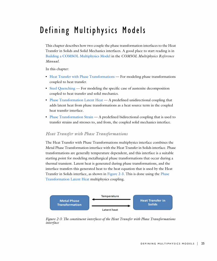
The Heat Transfer with Phase Transformations multiphysics interface combines the Metal Phase Transformation interface with the Heat Transfer in Solids interface. Phase transformations are generally temperature dependent, and this interface is a suitable starting point for modeling metallurgical phase transformations that occur during a thermal transient. Latent heat is generated during phase transformations, and the interface transfers this generated heat to the heat equation that is used by the Heat Transfer in Solids interface, as shown in Figure 2-3. This is done using the Phase Transformation Latent Heat multiphysics coupling.

Figure 2-3: The constituent interfaces of the Heat Transfer with Phase Transformations interface

D E F I N I N G M U L T I P H Y S I C S M O D E L S | 25

26 | C H A P T E R

Steel Quenching

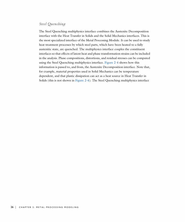
The Steel Quenching multiphysics interface combines the Austenite Decomposition interface with the Heat Transfer in Solids and the Solid Mechanics interfaces. This is the most specialized interface of the Metal Processing Module. It can be used to study heat treatment processes by which steel parts, which have been heated to a fully austenitic state, are quenched. The multiphysics interface couples the constituent interfaces so that effects of latent heat and phase transformation strains can be included in the analysis. Phase compositions, distortions, and residual stresses can be computed using the Steel Quenching multiphysics interface. Figure 2-4 shows how this information is passed to, and from, the Austenite Decomposition interface. Note that, for example, material properties used in Solid Mechanics can be temperature dependent, and that plastic dissipation can act as a heat source in Heat Transfer in Solids (this is not shown in Figure 2-4). The Steel Quenching multiphysics interface


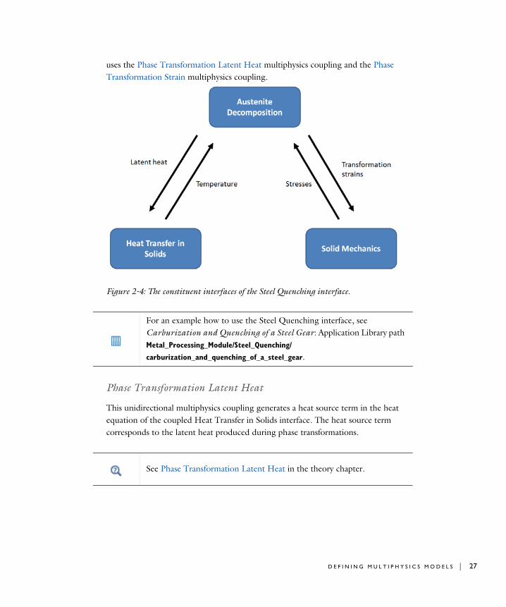
uses the Phase Transformation Latent Heat multiphysics coupling and the Phase Transformation Strain multiphysics coupling.

Figure 2-4: The constituent interfaces of the Steel Quenching interface.

Phase Transformation Latent Heat

This unidirectional multiphysics coupling generates a heat source term in the heat equation of the coupled Heat Transfer in Solids interface. The heat source term corresponds to the latent heat produced during phase transformations.

For an example how to use the Steel Quenching interface, see Carburization and Quenching of a Steel Gear: Application Library path Metal_Processing_Module/Steel_Quenching/

carburization_and_quenching_of_a_steel_gear.

See Phase Transformation Latent Heat in the theory chapter.

D E F I N I N G M U L T I P H Y S I C S M O D E L S | 27

28 | C H A P T E R

Phase Transformation Strain

This bidirectional multiphysics coupling is used to transfer strains and stresses to, and from, the coupled Solid Mechanics interface.

• If Enable transformation-induced plasticity is selected, the stress tensor from the Solid Mechanics interface is used to compute TRIP strains during phase transformations. These strains are used by the Solid Mechanics interface as an inelastic strain contribution.

• If Enable thermal strains is selected, the thermal strains are used by the Solid Mechanics interface as an inelastic contribution.

• If Enable phase plasticity is selected, and if the Plasticity subnode under Linear Elastic

Material is used by the coupled Solid Mechanics interface, the equivalent plastic strain is transferred to the phase transformation interface. This way, the individual hardening function for each phase can be evaluated.

When you use this coupling, you should not use the Thermal Expansion node to compute thermal strains to be used in the Solid Mechanics interface.


S e l e c t i n g D i s c r e t i z a t i o n s

Phase Transformation Modeling

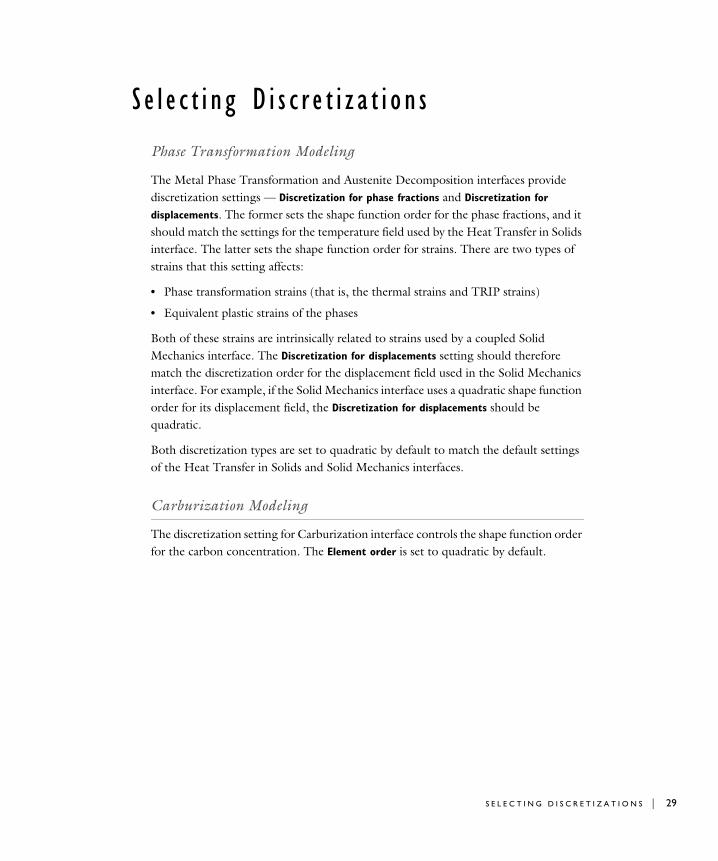
The Metal Phase Transformation and Austenite Decomposition interfaces provide discretization settings — Discretization for phase fractions and Discretization for

displacements. The former sets the shape function order for the phase fractions, and it should match the settings for the temperature field used by the Heat Transfer in Solids interface. The latter sets the shape function order for strains. There are two types of strains that this setting affects:

• Phase transformation strains (that is, the thermal strains and TRIP strains)

• Equivalent plastic strains of the phases

Both of these strains are intrinsically related to strains used by a coupled Solid Mechanics interface. The Discretization for displacements setting should therefore match the discretization order for the displacement field used in the Solid Mechanics interface. For example, if the Solid Mechanics interface uses a quadratic shape function order for its displacement field, the Discretization for displacements should be quadratic.

Both discretization types are set to quadratic by default to match the default settings of the Heat Transfer in Solids and Solid Mechanics interfaces.

Carburization Modeling

The discretization setting for Carburization interface controls the shape function order for the carbon concentration. The Element order is set to quadratic by default.

S E L E C T I N G D I S C R E T I Z A T I O N S | 29

30 | C H A P T E R

U s i n g E f f e c t i v e Ma t e r i a l P r op e r t i e s

When a material undergoes phase transformations during a thermal transient, its material properties will change. The properties are typically temperature dependent and tend to be phase dependent, too. For example, the initial yield stress at a given temperature will be higher in martensite than in ferrite — two metallurgical phases that appear during hardening of steel. When the Metal Phase Transformation or Austenite Decomposition interface is used with Heat Transfer in Solids or Solid Mechanics, it can compute effective material properties that can be utilized by these interfaces. The benefit is that the Heat Transfer in Solids and Solid Mechanics interfaces themselves do not need to perform phase averaging of the material properties that are used.

You can generate a compound material that can be used by other physics interfaces as a domain material. The compound material is created if you use the Create Compound

Material option at the physics interface level. This material contains effective material properties that are computed from the corresponding material properties defined for each phase.

Compound Material Properties

Note that if Enable phase plasticity has been selected at the physics interface level, the User defined option should be used for the Isotropic

hardening model in the Plasticity node in Solid Mechanics.


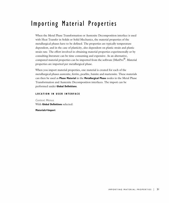
Impo r t i n g Ma t e r i a l P r op e r t i e s

When the Metal Phase Transformation or Austenite Decomposition interface is used with Heat Transfer in Solids or Solid Mechanics, the material properties of the metallurgical phases have to be defined. The properties are typically temperature dependent, and in the case of plasticity, also dependent on plastic strain and plastic strain rate. The effort involved in obtaining material properties experimentally or by consulting literature can be time consuming and expensive. As an alternative, computed material properties can be imported from the software JMatPro®. Material properties are imported per metallurgical phase.

When you import material properties, one material is created for each of the metallurgical phases austenite, ferrite, pearlite, bainite and martensite. These materials can then be used as Phase Material in the Metallurgical Phase nodes in the Metal Phase Transformation and Austenite Decomposition interfaces. The import can be performed under Global Definitions.

L O C A T I O N I N U S E R I N T E R F A C E

Context MenusWith Global Definitions selected:

Materials>Import

I M P O R T I N G M A T E R I A L P R O P E R T I E S | 31

32 | C H A P T E R

Mode l i n g C a r bu r i z a t i o n

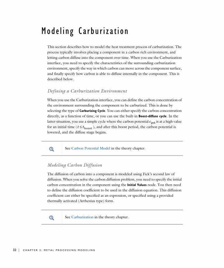
This section describes how to model the heat treatment process of carburization. The process typically involves placing a component in a carbon rich environment, and letting carbon diffuse into the component over time. When you use the Carburization interface, you need to specify the characteristics of the surrounding carburization environment, specify the way in which carbon can move across the component surface, and finally specify how carbon is able to diffuse internally in the component. This is described below.

Defining a Carburization Environment

When you use the Carburization interface, you can define the carbon concentration of the environment surrounding the component to be carburized. This is done by selecting the type of Carburizing Cycle. You can either specify the carbon concentration directly, as a function of time, or you can use the built-in Boost-diffuse cycle. In the latter situation, you use a simple cycle where the carbon potential cpot is at a high value for an initial time ( ), and after this boost period, the carbon potential is lowered, and the diffuse stage begins.

Modeling Carbon Diffusion

The diffusion of carbon into a component is modeled using Fick’s second law of diffusion. When you solve the carbon diffusion problem, you need to specify the initial carbon concentration in the component using the Initial Values node. You then need to define the diffusion coefficient to be used in the diffusion equation. This diffusion coefficient can either be specified as an expression, or specified using a provided thermally activated (Arrhenius type) form.

t tboost≤

See Carbon Potential Model in the theory chapter.

See Carburization in the theory chapter.


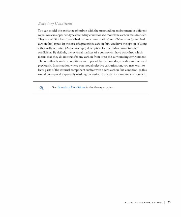
Boundary Conditions

You can model the exchange of carbon with the surrounding environment in different ways. You can apply two types boundary conditions to model the carbon mass transfer. They are of Dirichlet (prescribed carbon concentration) or of Neumann (prescribed carbon flux) types. In the case of a prescribed carbon flux, you have the option of using a thermally activated (Arrhenius type) description for the carbon mass transfer coefficient. By default, the external surfaces of a component have zero flux, which means that they do not transfer any carbon from or to the surrounding environment. The zero flux boundary conditions are replaced by the boundary conditions discussed previously. In a situation where you model selective carburization, you may want to leave parts of the external component surface with a zero carbon flux condition, as this would correspond to partially masking the surface from the surrounding environment.

See Boundary Conditions in the theory chapter.

M O D E L I N G C A R B U R I Z A T I O N | 33

34 | C H A P T E R

Re f e r e n c e s

1. T. Holm, P. Olsson, and E. Troell (Eds.), “Steel and its heat treatment — A handbook”, Swerea IVF, Mölndal, 2012.


3

M e t a l P r o c e s s i n g T h e o r y

This chapter introduces you to the theory for the Metal Processing Module.

In this chapter:


• Phase Transformation Strains

• Phase Transformation Latent Heat

• Compound Material Properties

• Carburization

35

36 | C H A P T E R

Me t a l Pha s e T r a n s f o rma t i o n Th eo r y

In the following, the theory for the Metal Phase Transformation physics interface is described. This section also covers the theory for the Austenite Decomposition physics interface. These physics interfaces can be used to model metallurgical phase transformations in metals. They can be coupled to Heat Transfer in Solids and Solid Mechanics, where, for example, quenching of steel components can be performed.

3 : M E T A L P R O C E S S I N G T H E O R Y

Me t a l l u r g i c a l Pha s e T r a n s f o rma t i o n s

Definitions

The material consists of a number of metallurgical phases. The fraction of each phase i is denoted ξi. There are in general N phases, where

The initial phase fraction must be defined for each phase, and the sum of initial phase fractions should be one. At the onset of an analysis, some phases may not be present, and have zero initial phase fraction.

Each phase transformation describes how a source phase s transforms into a destination phase d. A phase transformation is formally defined by the rate at which the destination phase d forms at the expense of the source phase s. This can be expressed as

(3-1)

Note that this equation describes only a single contribution to the total rates at which the destination phase forms, and the source phase decomposes. With several simultaneous phase transformations, some phases may receive more than one contribution. As an example, consider the case of three phases and two phase transformations, where phase 1 transforms into phases 2 and 3. Using the terminology above, the total rate equations for the three phases can be expressed as

ξi

i 1=

N

1=

• The phase fractions are defined in the material frame.

• Because of the employed weighting scheme for the effective mass density of the compound material, the phase fractions become algebraic fractions.

• See Compound Material Properties.

As d→

As d→ ξ·d

ξ·s

–= =

ξ·1

A– 1 2→ A1 3→–=

M E T A L L U R G I C A L P H A S E T R A N S F O R M A T I O N S | 37

38 | C H A P T E R

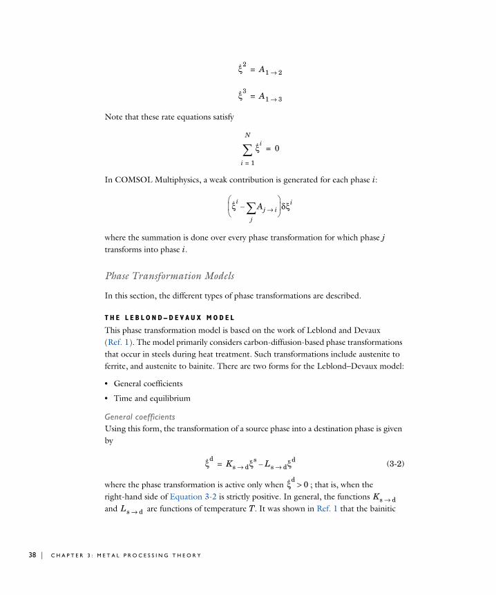
Note that these rate equations satisfy

In COMSOL Multiphysics, a weak contribution is generated for each phase i:

where the summation is done over every phase transformation for which phase j transforms into phase i.

Phase Transformation Models

In this section, the different types of phase transformations are described.

T H E L E B L O N D – D E V A U X M O D E L

This phase transformation model is based on the work of Leblond and Devaux (Ref. 1). The model primarily considers carbon-diffusion-based phase transformations that occur in steels during heat treatment. Such transformations include austenite to ferrite, and austenite to bainite. There are two forms for the Leblond–Devaux model:

• General coefficients

• Time and equilibrium

General coefficientsUsing this form, the transformation of a source phase into a destination phase is given by

(3-2)

where the phase transformation is active only when ; that is, when the right-hand side of Equation 3-2 is strictly positive. In general, the functions and are functions of temperature T. It was shown in Ref. 1 that the bainitic

ξ·2

A1 2→=

ξ·3

A1 3→=

ξ·i

i 1=

N

0=

ξ·i

Aj i→j–

δξi

ξ·d

Ks d→ ξs Ls d→ ξd–=

ξ·d0>

Ks d→Ls d→


transformation additionally depends on the rate of cooling, . In this case, the functions and are functions of both T and .

Time and equilibriumThis form is a special case of the general-coefficients form. The phase transformation is defined by an equilibrium phase fraction for the destination phase and a time constant . The phase transformation is given by

(3-3)

where the phase transformation is active only when ; that is, when the right side of Equation 3-3 is strictly positive. The equilibrium phase fraction and the time constant are typically functions of temperature.

T H E J O H N S O N – M E H L – A V R A M I – K O L M O G O R O V ( J M A K ) M O D E L

This phase transformation model is based on the work by Leblond and others (Ref. 3). This model can be viewed as a generalization of the Leblond–Devaux model. It is based on an Avrami law of the form

(3-4)

The equilibrium phase fraction , the time constant and the Avrami constant are typically functions of temperature. On rate form, Equation 3-4 can be

expressed as

(3-5)

where the explicit time dependence has been eliminated. The phase transformation is active only when ; that is, when the right side of Equation 3-5 is strictly positive. For the special case of , the equation reduces to the time-and-equilibrium form of the Leblond–Devaux model (Equation 3-3). The JMAK phase transformation model in Equation 3-5 has a mathematical disadvantage in that an initial destination phase fraction equal to zero will yield a trivial zero solution, as the logarithm will evaluate to zero. There are different ways to circumvent this problem. One way is to require the initial phase fraction be assigned a small, but finite, value. Another way is to modify the rate equation itself, so that a zero initial phase fraction does not yield a

T·

Ks d→ Ls d→ T·

ξeqd

τs d→

ξ·d ξeq

d ξd–

τs d→--------------------=

ξ·d

0>ξeq

d

τs d→

ξd ξeqd 1 t

τs d→--------------

ns d→

–

exp–

=

ξeqd τs d→

ns d→

ξ·d ξeq

d ξd–

τs d→--------------------ns d→ 1 ξd

ξeqd

--------–

ln–

1 1ns d→

---------------–

=

ξ·d

0>ns d→ 1=


40 | C H A P T E R

trivial zero solution. In the phase transformation interfaces, the JMAK phase transformation model in Equation 3-5 is modified for small values on the phase fraction . Below a certain threshold, the argument for the logarithm is modified so that the logarithm does not produce a zero value. This threshold phase fraction is set to 10-6 by default.

T H E K O I S T I N E N – M A R B U R G E R M O D E L

This phase transformation model was developed by Koistinen and Marburger (Ref. 2) to model the diffusionless (displacive) austenite-martensite transformation in iron-carbon alloys and carbon steels. The onset of the transformation, which only occurs on cooling, is characterized by a critical start temperature — the martensite start temperature Ms. Above this temperature, no transformation from austenite (the source phase) to martensite (the destination phase) occurs. Below Ms, the amount of formed martensite is proportional to the undercooling below Ms, given by Ms − T. On rate form, the Koistinen–Marburger equation can be written

(3-6)

where β is the Koistinen–Marburger coefficient. Note that the transformation of austenite into martensite only occurs below Ms and only during cooling (that is, when

). To make the onset of martensitic transformation numerically smooth, a parameter ΔMs is used. The smoothing parameter defines a smoothed Heaviside function that makes the onset of martensitic transformation gradual. The parameter should be chosen small enough that the start temperature characteristic is retained. Assuming a constant cooling rate and that the phase fraction of austenite at Ms is , the rate equation can be integrated to

(3-7)

This integrated form is commonly found in the literature. The rate form of Equation 3-6 is more general, and from a computational standpoint it is more suitable for implementation. The rate form is therefore used in the phase transformation interfaces.

ξd

The phase fraction threshold variable used by the JMAK phase transformation model can be modified in the Equation View of the Phase

Transformation node. Typically, the default value of 10−6 should not have to be changed.

ξ·d

ξsβT·

–=

T·

0<

ξ0s

ξd ξ0s 1 β Ms T–( )–( )exp–( )=


U S E R D E F I N E D

Using this option, other types of phase transformations can be defined. A user-defined phase transformation assumes that a source phase decomposes into a destination phase according to Equation 3-1.


42 | C H A P T E R

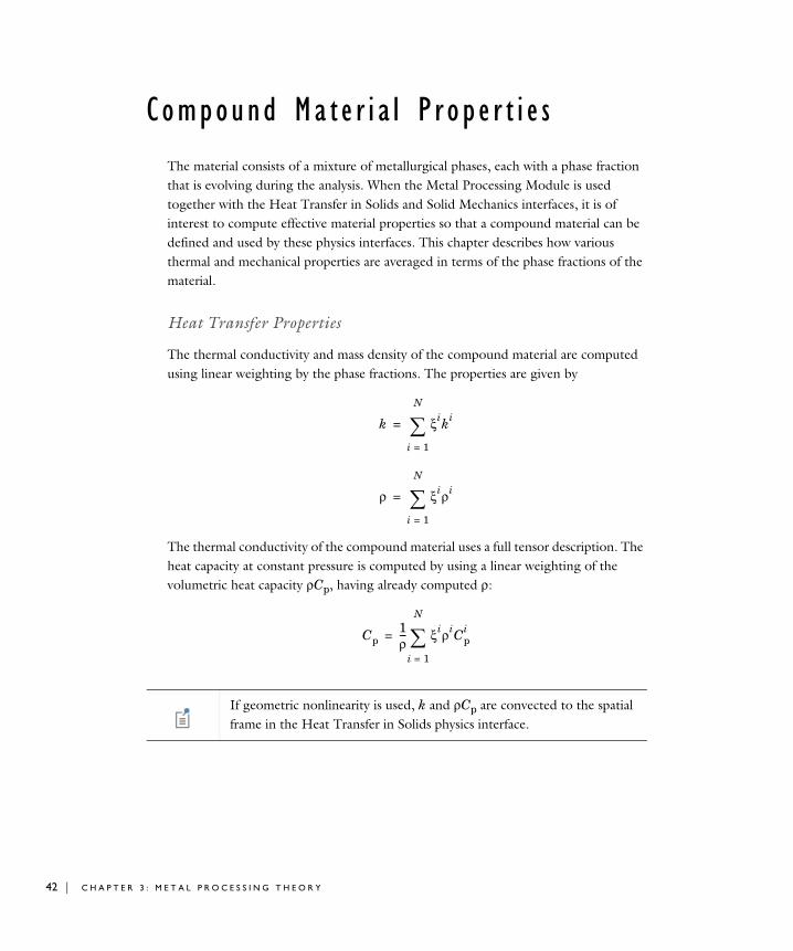
Compound Ma t e r i a l P r op e r t i e s

The material consists of a mixture of metallurgical phases, each with a phase fraction that is evolving during the analysis. When the Metal Processing Module is used together with the Heat Transfer in Solids and Solid Mechanics interfaces, it is of interest to compute effective material properties so that a compound material can be defined and used by these physics interfaces. This chapter describes how various thermal and mechanical properties are averaged in terms of the phase fractions of the material.

Heat Transfer Properties

The thermal conductivity and mass density of the compound material are computed using linear weighting by the phase fractions. The properties are given by

The thermal conductivity of the compound material uses a full tensor description. The heat capacity at constant pressure is computed by using a linear weighting of the volumetric heat capacity ρCp, having already computed ρ:

k ξiki

i 1=

N

=

ρ ξiρi

i 1=

N

=

Cp1ρ--- ξiρiCp

i

i 1=

N

=

If geometric nonlinearity is used, k and ρCp are convected to the spatial frame in the Heat Transfer in Solids physics interface.


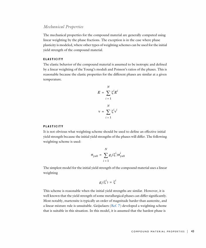
Mechanical Properties

The mechanical properties for the compound material are generally computed using linear weighting by the phase fractions. The exception is in the case where phase plasticity is modeled, where other types of weighting schemes can be used for the initial yield strength of the compound material.

E L A S T I C I T Y

The elastic behavior of the compound material is assumed to be isotropic and defined by a linear weighting of the Young’s moduli and Poisson’s ratios of the phases. This is reasonable because the elastic properties for the different phases are similar at a given temperature.

P L A S T I C I T Y

It is not obvious what weighting scheme should be used to define an effective initial yield strength because the initial yield strengths of the phases will differ. The following weighting scheme is used:

The simplest model for the initial yield strength of the compound material uses a linear weighting

This scheme is reasonable when the initial yield strengths are similar. However, it is well known that the yield strength of some metallurgical phases can differ significantly. Most notably, martensite is typically an order of magnitude harder than austenite, and a linear mixture rule is unsuitable. Geijselaers (Ref. 7) developed a weighting scheme that is suitable in this situation. In this model, it is assumed that the hardest phase is

E ξiEi

i 1=

N

=

ν ξiνi

i 1=

N

=

σys0 gi ξi( )σys0i

i 1=

N

=

gi ξi( ) ξi=

C O M P O U N D M A T E R I A L P R O P E R T I E S | 43

44 | C H A P T E R

considerably harder than the softest phase. Assuming that the hard phase is m and the soft phase is γ, the Geijselaers weighting scheme is given by

with

The hardening function for the compound material is defined using the linear weighting

(3-8)

where is the equivalent plastic strain of the phase.

E Q U I V A L E N T P L A S T I C S T R A I N S

In Equation 3-8, the hardening function for each individual phase depends on equivalent plastic strain. If we denote the equivalent plastic strain of the compound material , we must define how the equivalent of each phase evolves with this strain. The simplest assumption is to use the evolution equation

which is to say that the equivalent plastic strain of phase i follows that of the compound material. If phase transformation and mechanical straining occur simultaneously, the equivalent plastic strain of the diminishing source phase of the phase transformation can be taken to follow that of the compound material, and this is the behavior in the phase transformation physics interfaces. However, for a phase which is increasing in fraction during plastic straining, this assumption is questionable. Leblond (Ref. 6) derived an evolution equation for the equivalent plastic strain, which is suitable for the

gi ξi( ) ξi, i m≠

fi ξi( ), i=m

=

fm ξm( ) ξm C 2 1 C–( )ξm 1 C–( ) ξm( )2

–+( )=

C 1.383σys0

γ

σys0m

-----------=

σh ξiσhi εpe

i( )

i 1=

N

=

εpei

εpe εpei

ε·pei

ε·pe=


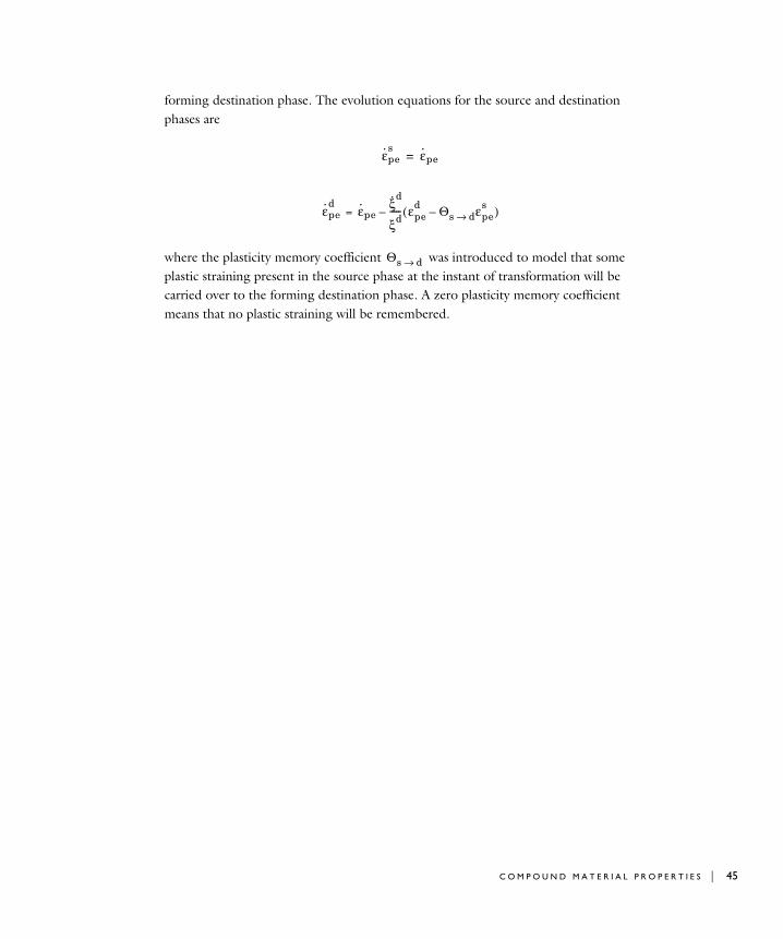
forming destination phase. The evolution equations for the source and destination phases are

where the plasticity memory coefficient was introduced to model that some plastic straining present in the source phase at the instant of transformation will be carried over to the forming destination phase. A zero plasticity memory coefficient means that no plastic straining will be remembered.

ε·pes

ε·pe=

ε·ped

= ε·peξ·

d

ξd----- εpe

d Θs d→ εpes

–( )–

Θs d→

C O M P O U N D M A T E R I A L P R O P E R T I E S | 45

46 | C H A P T E R

Pha s e T r a n s f o rma t i o n S t r a i n s

We consider two types of strains that appear during a thermal transient involving metallurgical phase transformations. These strains originate from:

• Thermal expansion

• Transformation induced plasticity (TRIP)

Other inelastic strains may also be present during a thermal transient, such as plastic strains or creep strains.

Thermal Expansion

Thermal expansion for the compound material is given by a phase fraction weighted sum of the thermal expansion of each phase:

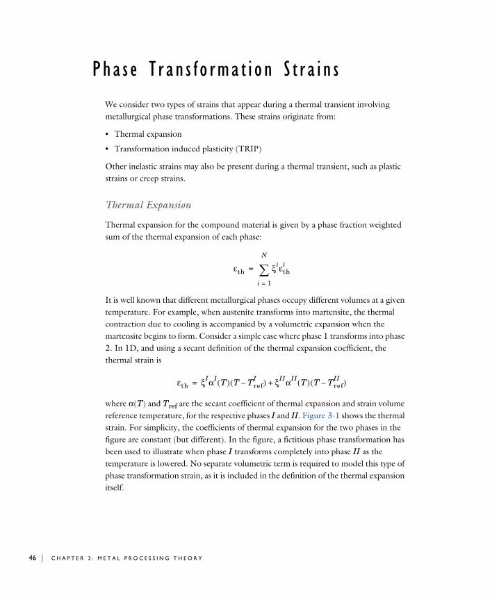
It is well known that different metallurgical phases occupy different volumes at a given temperature. For example, when austenite transforms into martensite, the thermal contraction due to cooling is accompanied by a volumetric expansion when the martensite begins to form. Consider a simple case where phase 1 transforms into phase 2. In 1D, and using a secant definition of the thermal expansion coefficient, the thermal strain is

where α(T) and Tref are the secant coefficient of thermal expansion and strain volume reference temperature, for the respective phases I and II. Figure 3-1 shows the thermal strain. For simplicity, the coefficients of thermal expansion for the two phases in the figure are constant (but different). In the figure, a fictitious phase transformation has been used to illustrate when phase I transforms completely into phase II as the temperature is lowered. No separate volumetric term is required to model this type of phase transformation strain, as it is included in the definition of the thermal expansion itself.

εth ξiεthi

i 1=

N

=

εth ξIαI T( ) T TrefI

–( ) ξIIαII T( ) T TrefII

–( )+=


Figure 3-1: Thermal strain during phase transformation.

Transformation-Induced Plasticity

Plastic strains in metals result from deviatoric stresses that exceed the yield strength of the material. However, during phase transformations, inelastic strains may appear already at very small stress levels. This transformation-induced plasticity (TRIP) is therefore different from classical plasticity in that it does not involve a yield criterion and that it appears at stress levels that would otherwise be insufficient to cause plastic straining even in the softest of the phases. A description of TRIP strain rate, common in the literature (see, for example, Ref. 3), is

where the strain rate is proportional to the deviatoric part of the second Piola–Kirchhoff stress tensor S through the transformation induced plasticity parameter

, the derivative of the saturation function Φ(ξd), and the rate of the destination phase . Values for the transformation-induced plasticity parameter will depend on the type of phase transformation. It can depend on, for example, carbon content and temperature (see Ref. 4). Several propositions exist for the saturation

ε· tp s, d→32---Ks d→

TRIP dΦ ξd( )

dξd-------------------ξ·

ddev S( )⋅ ⋅=

Ks d→TRIP

ξ·d

Ks d→TRIP

P H A S E T R A N S F O R M A T I O N S T R A I N S | 47

48 | C H A P T E R

functions; see Table 3-1 and Ref. 9. Through the user-defined option, you can define the derivative of the saturation function.

The total TRIP strain rate is given by

Total Strain Contribution

When thermal and TRIP strains are computed, they can be used in a Solid Mechanics interface as an inelastic strain contribution. The contributions from thermal and TRIP strains are added to form a total strain contribution. In the Solid Mechanics interface, this contribution is used additively in the case of an additive strain definition or used to form an inelastic-deformation-gradient contribution in the case of geometric nonlinearity with nonlinear strains; see Inelastic Strain Contributions. In the latter case, the contribution is used multiplicatively.

TABLE 3-1: SATURATION FUNCTIONS FOR THE TRIP STRAIN RATE

TYPE EXPRESSION

Abrassart

Desalos ξd(2-ξd)

Leblond ξd(1-lnξd)) for ξd>0.03, zero otherwise

Tanaka ξd

ξd 3 2 ξd–( )

ε· tp ε· tp s, d→

s d→=


Pha s e T r a n s f o rma t i o n L a t e n t Hea t

The heat rate Q0 that is released during a phase transformation is characterized by the enthalpy per unit volume (see Ref. 4). The heat rate that is associated with the transformation of a source phase into a destination phase can be expressed as

(3-9)

The heat rates that result from each phase transformation are added, and they can be used as a heat source when solving the heat equation. A weak contribution is added to the weak form of the heat equation:

where is the sum of the contributions Q0 from each phase transformation (Equation 3-9), and T is the temperature degree of freedom used in the Heat Transfer in Solids interface.

ΔHs d→

Q0 ΔHs d→ ξ·d

=

Qˆ

0δ T( )

Qˆ

0

P H A S E T R A N S F O R M A T I O N L A T E N T H E A T | 49

50 | C H A P T E R

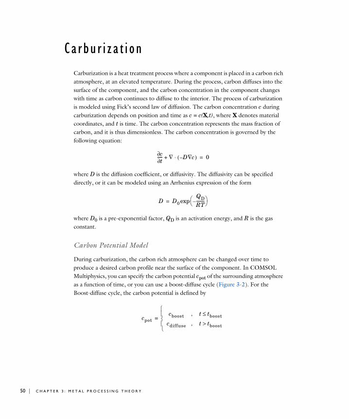
Ca r bu r i z a t i o n

Carburization is a heat treatment process where a component is placed in a carbon rich atmosphere, at an elevated temperature. During the process, carbon diffuses into the surface of the component, and the carbon concentration in the component changes with time as carbon continues to diffuse to the interior. The process of carburization is modeled using Fick’s second law of diffusion. The carbon concentration c during carburization depends on position and time as c = c(X,t), where X denotes material coordinates, and t is time. The carbon concentration represents the mass fraction of carbon, and it is thus dimensionless. The carbon concentration is governed by the following equation:

where D is the diffusion coefficient, or diffusivity. The diffusivity can be specified directly, or it can be modeled using an Arrhenius expression of the form

where D0 is a pre-exponential factor, QD is an activation energy, and R is the gas constant.

Carbon Potential Model

During carburization, the carbon rich atmosphere can be changed over time to produce a desired carbon profile near the surface of the component. In COMSOL Multiphysics, you can specify the carbon potential cpot of the surrounding atmosphere as a function of time, or you can use a boost-diffuse cycle (Figure 3-2). For the Boost-diffuse cycle, the carbon potential is defined by

c∂t∂

----- ∇ D c∇–( )⋅+ 0=

D D0QDRT--------–

exp=

cpotcboost , t tboost≤

cdiffuse , t tboost>

=


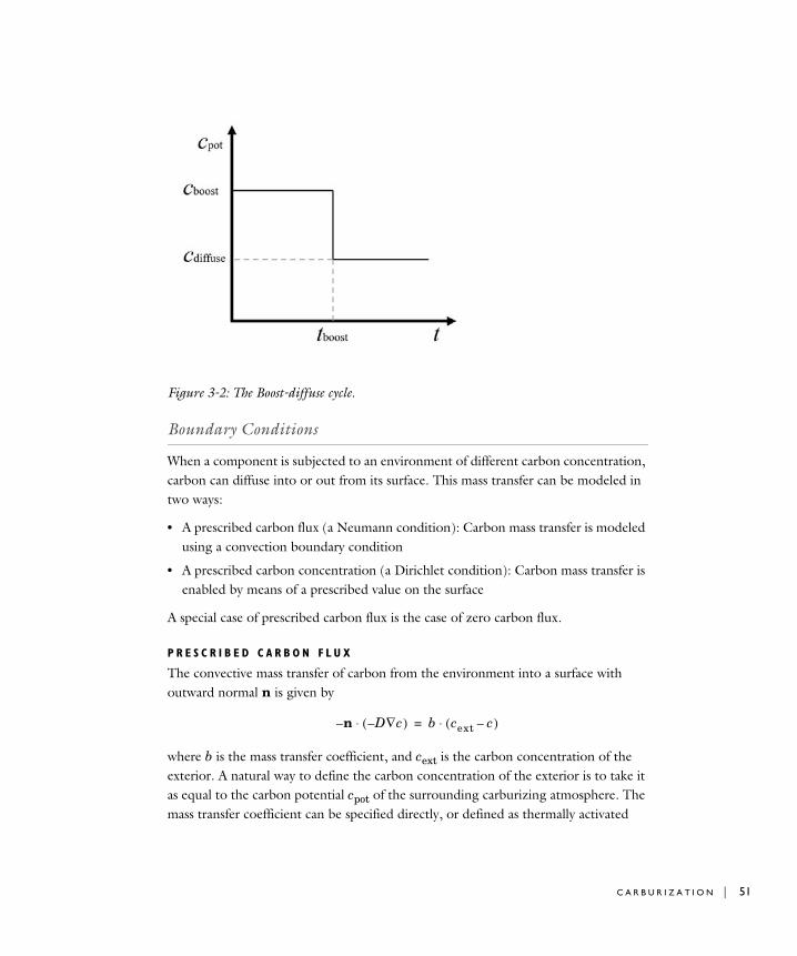
Figure 3-2: The Boost-diffuse cycle.

Boundary Conditions

When a component is subjected to an environment of different carbon concentration, carbon can diffuse into or out from its surface. This mass transfer can be modeled in two ways:

• A prescribed carbon flux (a Neumann condition): Carbon mass transfer is modeled using a convection boundary condition

• A prescribed carbon concentration (a Dirichlet condition): Carbon mass transfer is enabled by means of a prescribed value on the surface

A special case of prescribed carbon flux is the case of zero carbon flux.

P R E S C R I B E D C A R B O N F L U X

The convective mass transfer of carbon from the environment into a surface with outward normal n is given by

where b is the mass transfer coefficient, and cext is the carbon concentration of the exterior. A natural way to define the carbon concentration of the exterior is to take it as equal to the carbon potential cpot of the surrounding carburizing atmosphere. The mass transfer coefficient can be specified directly, or defined as thermally activated

n– D∇c–( )⋅ b cext c–( )⋅=

C A R B U R I Z A T I O N | 51

52 | C H A P T E R

where b0 is a pre-exponential factor and Qb is an activation energy. In a given situation, these quantities would have to be estimated or measured experimentally.

P R E S C R I B E D C A R B O N C O N C E N T R A T I O N

A simple way to model the carbon exchange is to simply prescribe the carbon concentration at the surface of the component to be equal to the carbon concentration of the exterior. This modeling approach avoids having to characterize the carbon mass transfer, but it may instead exaggerate it because the surface will be saturated.

b b0QbRT--------–

exp=


Re f e r e n c e s

1. J.B. Leblond and J.C. Devaux, “A new kinetic model for anisothermal metallurgical phase transformations in steels including effect of austenite grain size”, Acta Metall., vol. 32, no. 1, pp. 137–146, 1984.

2. D.P. Koistinen and R.E. Marburger, “A general equation prescribing the extent of the austenite-martensite transformation in pure iron-carbon alloys and plain carbon steels”, Acta Metall., vol. 7, no. 1, pp. 59–60, 1959.

3. J.B. Leblond, G. Mottet, J. Devaux, and J.C. Devaux, “Mathematical models of anisothermal phase transformations in steels, and predicted plastic behaviour”, Mat. Sci. Tech., vol. 1, no. 10, pp. 815–822, 1985.

4. B. Liscic, H.M. Tensi, L.C.F. Canale, and G.E. Totten (Eds.), Quenching theory and technology, CRC Press, Taylor & Francis Group, 2010.

5. J.B. Leblond, J. Devaux, and J.C. Devaux, “Mathematical modelling of transformation plasticity in steels I: Case of ideal-plastic phases”, Int. J. Plast., vol. 5, pp. 551–572, 1989.

6. J.B. Leblond, “Mathematical modelling of transformation plasticity in steels II: Coupling with strain hardening phenomena”, Int. J. Plast., vol. 5, pp. 573–591, 1989.

7. H.J.M. Geijselaers, Numerical simulation of stresses due to solid state transformations: The simulation of laser hardening, doctoral dissertation, Univ. of Twente, Enschede, 2003.

8. J. Gyhlesten Back, Modelling and characterisation of the martensite formation in low-alloyed carbon steels, licentiate thesis, Luleå Univ. of Technology, Luleå, 2017.

9. S. Boettcher, M. Böhm, and M. Wolff, A comprehensive model of thermo-elasto-plasticity with phase transitions in steel, Zentrum für Technomathematik, Universität Bremen, 2013.

R E F E R E N C E S | 53

54 | C H A P T E R

4

M e t a l P h a s e T r a n s f o r m a t i o n

This chapter describes the Metal Phase Transformation Interface ( ) and its functionality. It is found under the Heat Transfer>Metal Processing branch ( ) when adding a physics interface.

55

56 | C H A P T E R

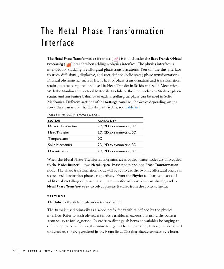
Th e Me t a l Pha s e T r a n s f o rma t i o n I n t e r f a c e

The Metal Phase Transformation interface ( ) is found under the Heat Transfer>Metal

Processing ( ) branch when adding a physics interface. The physics interface is intended for studying metallurgical phase transformations. You can use this interface to study diffusional, displacive, and user-defined (solid state) phase transformations. Physical phenomena, such as latent heat of phase transformation and transformation strains, can be computed and used in Heat Transfer in Solids and Solid Mechanics. With the Nonlinear Structural Materials Module or the Geomechanics Module, plastic strains and hardening behavior of each metallurgical phase can be used in Solid Mechanics. Different sections of the Settings panel will be active depending on the space dimension that the interface is used in, see Table 4-1.

When the Metal Phase Transformation interface is added, three nodes are also added to the Model Builder — two Metallurgical Phase nodes and one Phase Transformation node. The phase transformation node will be set to use the two metallurgical phases as source and destination phases, respectively. From the Physics toolbar, you can add additional metallurgical phases and phase transformations. You can also right-click Metal Phase Transformation to select physics features from the context menu.

S E T T I N G S

The Label is the default physics interface name.

The Name is used primarily as a scope prefix for variables defined by the physics interface. Refer to such physics interface variables in expressions using the pattern <name>.<variable_name>. In order to distinguish between variables belonging to different physics interfaces, the name string must be unique. Only letters, numbers, and underscores (_) are permitted in the Name field. The first character must be a letter.

TABLE 4-1: PHYSICS INTERFACE SECTIONS.

SECTION AVAILABILITY

Material Properties 2D, 2D axisymmetric, 3D

Heat Transfer 2D, 2D axisymmetric, 3D

Temperature 0D

Solid Mechanics 2D, 2D axisymmetric, 3D

Discretization 2D, 2D axisymmetric, 3D

4 : M E T A L P H A S E T R A N S F O R M A T I O N

The default Name (for the first physics interface in the model) is metp.

M A T E R I A L P R O P E R T I E S

You have the option of letting the physics interface compute effective thermal and mechanical material properties, based on the corresponding properties and fractions of the individual metallurgical phases. Select the Compute effective thermal properties check box to let the physics interface compute effective thermal properties. Select the Compute effective mechanical properties check box to let the physics interface compute effective mechanical properties. You can use the computed effective material properties to create a compound material that can be used in other physics interfaces as a domain material. Select the Create Compound Material to create a compound material. This material is created at the component level.

H E A T T R A N S F E R

Phase transformations are inherently temperature dependent. Select the temperature field to use from the Temperature list. If you want to consider the release or absorption of latent heat during phase transformations, select the Enable phase transformation

latent heat check box. You can then define values for the latent heat at each of the phase transformation nodes. By default, the check box is not selected.

T E M P E R A T U R E

Phase transformations are inherently temperature dependent. Enter an expression for the temperature to use.

S O L I D M E C H A N I C S

This section contains settings that affect various strains that accompany phase transformations. Select the Enable transformation-induced plasticity check box if you want to include this type of transformation strain in your analysis. The Enable thermal

strains and Enable phase plasticity check boxes are visible only if you have selected the Compute effective mechanical properties check box in the Material Properties section. Select Enable thermal strains if you want to include thermal strains in your analysis.

A compound material that is generated from an Austenite Decomposition interface (audc) will be given the tag audcmat.

The two sections Heat Transfer and Temperature are mutually exclusive, and which one is active is determined by the space dimension.

T H E M E T A L P H A S E T R A N S F O R M A T I O N I N T E R F A C E | 57

58 | C H A P T E R

Note that the thermal strains will include both pure thermal strains as well as strains that arise from volumetric differences between different metallurgical phases. Select the Enable phase plasticity check box if you want to allow for plasticity in the individual phases. By default, none of the three check boxes in this section are selected.

D I S C R E T I Z A T I O N

The discretizations for phase fractions and displacements can be set independently using the Discretization for phase fractions and Discretization for displacements lists. In general, the Discretization for displacements setting should match the discretization order used for the displacement field in the Solid Mechanics interface. By default, Linear is selected for phase fractions and Quadratic for displacements.

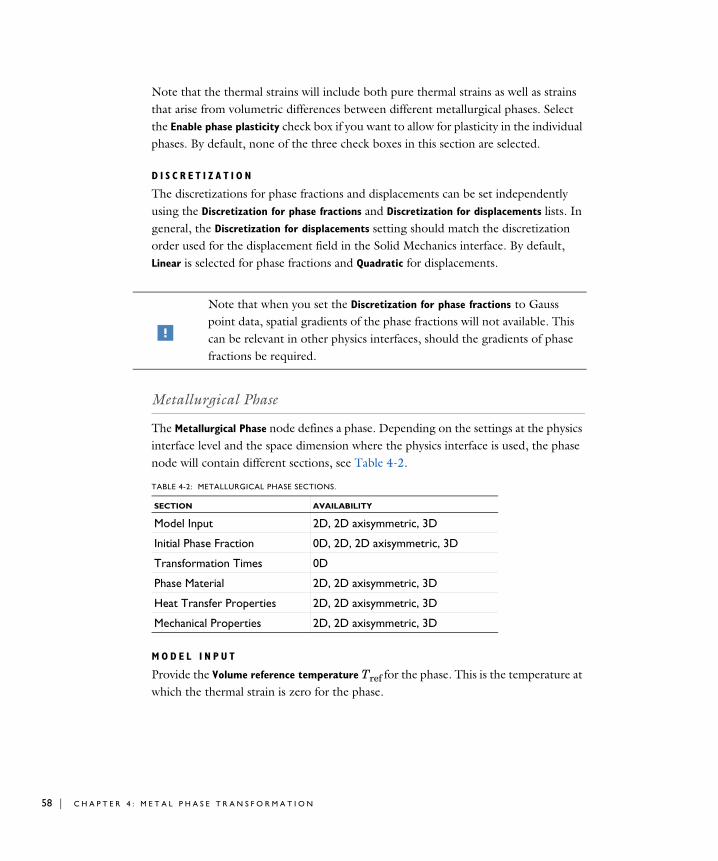
Metallurgical Phase

The Metallurgical Phase node defines a phase. Depending on the settings at the physics interface level and the space dimension where the physics interface is used, the phase node will contain different sections, see Table 4-2.

M O D E L I N P U T

Provide the Volume reference temperature Tref for the phase. This is the temperature at which the thermal strain is zero for the phase.

Note that when you set the Discretization for phase fractions to Gauss point data, spatial gradients of the phase fractions will not available. This can be relevant in other physics interfaces, should the gradients of phase fractions be required.

TABLE 4-2: METALLURGICAL PHASE SECTIONS.


Model Input 2D, 2D axisymmetric, 3D

Initial Phase Fraction 0D, 2D, 2D axisymmetric, 3D

Transformation Times 0D

Phase Material 2D, 2D axisymmetric, 3D

Heat Transfer Properties 2D, 2D axisymmetric, 3D

Mechanical Properties 2D, 2D axisymmetric, 3D


I N I T I A L P H A S E F R A C T I O N

Define the Initial phase fraction for the phase. This fraction should be a value between zero and one, and you have to ensure that the initial phase fractions for all the phases in your analysis sum to one.

T R A N S F O R M A T I O N T I M E S

If you select Compute transformation times, you can store the times and temperatures during an analysis, corresponding to reaching specified target phase fractions. Enter

a list of Target phase fractions in the table. Whether transformation times and temperatures are recorded depends on if the phase fraction is increasing or decreasing during the analysis. Select Decreasing phase fraction if the phase fraction is expected to reach the specified target values when it is decreasing.

P H A S E M A T E R I A L

From the Phase material list, you select the material that defines the material properties for the phase. This section is visible only if at least one of the Compute effective thermal

properties or the Compute effective mechanical properties check boxes has been selected at the physics interface level. You can create a material at the component level by using Create Phase Material. When you define material properties for the phase, From material will refer to the material that you have selected from the Phase material list.

• The initial fractions for the metallurgical phases are named metp.phase1.xi0, metp.phase2.xi0, and so on.

• The current phase fractions are correspondingly named metp.phase1.xi and metp.phase2.xi.

t̂

Tˆ

ξ̂

If the second Target phase fraction in the table is reached for a Metallurgical Phase (phase4) in an Austenite Decomposition interface (audc), the corresponding transformation time and temperature will be audc.phase4.time_2 and audc.phase4.temperature_2.

A phase material that is generated from a Metallurgical Phase (phase2) in an Austenite Decomposition interface (audc) will be given the tag audcphase2mat.


60 | C H A P T E R

H E A T T R A N S F E R P R O P E R T I E S

If the Compute effective thermal properties has been selected at the physics interface level, you must define the thermal properties for the phase. The default Thermal

conductivity k, Density ρ, and Heat Capacity at constant pressure Cp, use values From

material. The From material option refers to the selected material from the Phase

Material list. For User defined, enter values or expressions for these properties.

M E C H A N I C A L P R O P E R T I E S

If the Compute effective mechanical properties has been selected at the physics interface level, you must define mechanical properties for the phase. The default Young’s modulus E and Poisson’s ratio ν use values From material. For User defined, enter values or expressions for these properties.

If Enable thermal strains has been selected at the physics interface level, you have to define the Secant coefficient of thermal expansion α for the phase. By default, the value is taken From material. For User defined, enter a value or expression.

If Enable phase plasticity has been selected at the physics interface level, you have to define the plastic behavior of the phase. The default Initial yield stress σys0 uses a value From material. For User defined, enter another value or expression for initial yield stress. Initial yield stresses for phases can be weighted differently. This is useful when initial yield stresses for the phases in the model are very different. Select a Weight factor for

yield stress — Linear, Geijselaers, or User defined. If Geijselaers is selected, you also need to specify a Soft phase, which is considered plastically soft in comparison to this phase. You should typically use this to give a stronger weight to martensite (hard) in relation to austenite (soft).

Select the Isotropic hardening model — Perfectly plastic, Linear, or User defined to define the hardening behavior of the phase.

LinearSpecify the Isotropic hardening modulus ETiso. The default value is taken From material.

User definedFor User defined, enter another value or expression for the modulus. If a User defined isotropic hardening modulus is selected, you have to select the Hardening function. By default, the value is taken From material.


For User defined, enter a value or expression for the hardening function. The expression can depend, for example, on the equivalent plastic strain in the phase.

Phase Transformation

Depending on the settings at the physics interface level and the space dimension where the physics interface is used the phase transformation node will contain different sections, see Table 4-3.

P H A S E T R A N S F O R M A T I O N

The phase transformation defines how one phase forms (the destination phase) at the expense of another (the source phase). Select Source phase ξs and Destination phase ξd from the list of defined phases. Select a Phase transformation model — Leblond–Devaux, Johnson-Mehl-Avrami-Kolmogorov, Koistinen–Marburger or User defined.

Leblond–DevauxSelect Time and equilibrium or General coefficients. For Time and equilibrium, specify the Equilibrium phase fraction and Time constant . For General coefficients, specify the expressions for and . If applicable, select Define temperature

limits, and specify the Lower temperature limit Tl and the Upper temperature limit Tu.

Johnson–Mehl–Avrami–KolmogorovSpecify the Equilibrium phase fraction , the Time constant , and the Avrami

exponent . If applicable, select Define temperature limits, and specify the Lower

temperature limit Tl and the Upper temperature limit Tu.

Koistinen–MarburgerSpecify the Koistinen–Marburger coefficient β, the Martensite start temperature Ms, and a value for the Martensite start temperature smoothing ΔMs.

In a phase (phase4) of an Austenite Decomposition interface (audc), the equivalent plastic strain is audc.phase4.epe.

TABLE 4-3: PHASE TRANSFORMATION SECTIONS.


Phase Transformation 0D, 2D, 2D axisymmetric, 3D

Phase Transformation Latent Heat 2D, 2D axisymmetric, 3D

Phase Transformation Strain 2D, 2D axisymmetric, 3D

ξeqd τs d→

Ks d→ Ls d→

ξeqd τs d→

ns d→


62 | C H A P T E R

User definedSpecify the Phase transformation contribution . The expression defines the rate at which the destination phase forms, at the expense of the source phase.

P H A S E T R A N S F O R M A T I O N L A T E N T H E A T

This section is active if you have selected Enable phase transformation latent heat at the physics interface level. You can specify the latent heat that is released during the phase transformation.

P H A S E T R A N S F O R M A T I O N S T R A I N

The Transformation induced plasticity check box is available if you have selected Enable

transformation induced plasticity at the physics interface level. In case of transformation induced plasticity, specify the Transformation induced plasticity parameter and the Saturation function Φ.

The Plastic recovery for destination phase check box is available if the Enable thermal

strains has been selected at the physics interface level. If you have selected Plastic

recovery for destination phase, you can specify the Plastic memory coefficient . The default value is zero, which means that no plastic straining in the source phase will be carried over to the destination phase.

Transformation Condition

One or several Transformation Condition subnodes can be added to a Phase Transformation node. In the Transformation Condition subnode, specify a Boolean expression c that has to be satisfied for the Phase Transformation to take place. For example, if you have reason to prevent a phase transformation from occurring unless the temperature rate is negative, the expression could look like:

metp.Tt<0[K/s]

If several Transformation Condition subnodes are used, each separate condition has to be satisfied for the Phase Transformation to take place.

As d→

ΔHs d→

Ks d→TRIP

Θs d→


5

A u s t e n i t e D e c o m p o s i t i o n

This chapter describes the Austenite Decomposition Interface ( ) and its functionality. It is found under the Heat Transfer>Metal Processing branch ( ) when adding a physics interface.

63

64 | C H A P T E R

Th e Au s t e n i t e De c ompo s i t i o n I n t e r f a c e

The Austenite Decomposition interface ( ) is found under the Heat Transfer>Metal

Processing ( ) branch when adding a physics interface. The physics interface is intended for studying metallurgical phase transformations. You can use this interface to study diffusional, displacive, and user-defined (solid-solid) phase transformations. Physical phenomena, such as latent heat of phase transformation and transformation strains can be computed and used in Heat Transfer in Solids and Solid Mechanics. With the Nonlinear Structural Materials Module or the Geomechanics Module, plastic strains and hardening behavior of each metallurgical phase can be used in Solid Mechanics.

This interface is based on the Metal Phase Transformation interface. This chapter will only describe the nodes and settings that set the Austenite Decomposition interface apart from the Metal Phase Transformation interface. With regard to other settings at the physics interface level and feature level, see The Metal Phase Transformation Interface.

When the Austenite Decomposition interface is added, nine nodes are added to the Model Builder — five Metallurgical Phase nodes and four Phase Transformation nodes. The interface is tailored specifically to the decomposition of austenite into a combination of ferrite, pearlite, bainite, and martensite. The phase nodes are given names to reflect this:

• Austenite

• Ferrite

• Pearlite

• Bainite

• Martensite

The Initial Phase Fraction is set to one in the Austenite node, and zero in the other metallurgical phase nodes. Four Phase Transformation nodes are also created to define the relevant phase transformations:

• Austenite to Ferrite

• Austenite to Pearlite

5 : A U S T E N I T E D E C O M P O S I T I O N

• Austenite to Bainite

• Austenite to Martensite

The source and destination phases in each phase transformation are set to the corresponding phases that have been created. The Phase transformation model is set to Leblond–Devaux with General coefficients, except in Austenite to Martensite, where it is set to Koistinen–Marburger.

From the Physics toolbar, you can delete or disable metallurgical phases and phase transformations that are irrelevant in a given situation, and you can add additional metallurgical phases and phase transformations. You can also right-click Metal Phase

Transformation to select physics features from the context menu.

S E T T I N G S



The default Name (for the first physics interface in the model) is audc.

T H E A U S T E N I T E D E C O M P O S I T I O N I N T E R F A C E | 65

66 | C H A P T E R
5 : A U S T E N I T E D E C O M P O S I T I O N

6

C a r b u r i z a t i o n

This chapter describes the Carburization interface ( ) and its functionality. It is found under the Heat Transfer>Metal Processing branch ( ) when adding a physics interface.

67

68 | C H A P T E R

Th e C a r bu r i z a t i o n I n t e r f a c e

The Carburization interface ( ) is found under the Heat Transfer>Metal Processing ( ) branch when adding a physics interface. The physics interface is intended for modeling carburization processes during heat treatment. The carburization process is based on diffusion, and it is used to compute the evolving mass fraction of carbon when a component is exposed to a carbon rich atmosphere.

When the Carburization interface is added, three default nodes are added to the Model

Builder — a Carburization node, an Initial Values node, and a Zero Carbon Flux node.

S E T T I N G S



The default Name (for the first physics interface in the model) is carb.

T E M P E R A T U R E

Carbon diffusion is inherently temperature dependent. Select the temperature field to use from the Temperature list.

C A R B U R I Z I N G C Y C L E

This section contains settings for the carburization process. Select the carbon potential model to use from the Carbon potential model list. Select Boost-diffuse cycle if you want to model a two-stage carburization process, where a boost stage is followed by a diffuse stage. Define the Boost carbon potential cboost, the Diffuse carbon potential cdiffuse, and the Boost period tboost. Select User defined if you want to use your own expression for the carbon potential of the carburization process. Define the Carbon potential cpot.

Carburization

The Carburization node defines the carbon diffusion inside the domain.

6 : C A R B U R I Z A T I O N

C A R B O N D I F F U S I O N

From the Diffusion coefficient list you select the diffusion coefficient that is used in the diffusion equation. Select Arrhenius to define a thermally activated diffusion coefficient. Define the Pre-exponential factor D0 and the Activation energy QD. Select User defined to define the Diffusion coefficient D directly.

Carbon Flux

The Carbon Flux node is used to define the carbon exchange with the surrounding carbon atmosphere (the exterior).

C A R B O N M A S S T R A N S F E R

From the Carbon potential list, select the carbon potential of the exterior cext. Select Carbon potential to use the carbon potential defined at the physics interface level. Select User defined to define the carbon potential directly. From the Mass transfer coefficient list, select the mass transfer coefficient to be used to define the carbon flux. Select Arrhenius to define a thermally activated mass transfer coefficient. Define the Pre-exponential factor b0 and the Activation energy Qb. Select User defined to define the Mass transfer coefficient b directly.

Zero Carbon Flux

The Zero Carbon Flux node is used to define boundaries where no carbon exchange takes place with the exterior.

Carbon Concentration

The Carbon Concentration node is used to specify the carbon concentration at an exterior domain boundary.

C A R B O N C O N C E N T R A T I O N

From the list, select the carbon concentration c0. Select Carbon potential to use the carbon potential defined at the physics interface level. Select User defined to specify the carbon concentration c0 directly.

Initial Values

The Initial Values node is used to specify the initial carbon concentration c.

T H E C A R B U R I Z A T I O N I N T E R F A C E | 69

70 | C H A P T E R
6 : C A R B U R I Z A T I O N

7

M u l t i p h y s i c s I n t e r f a c e s a n d C o u p l i n g s

The Metal Processing Module contains predefined multiphysics interfaces to facilitate the coupling to Heat Transfer in Solids and Solid Mechanics interfaces. The physics interfaces are found under the Heat Transfer>Metal Processing branch ( ) when adding a physics interface — Heat Transfer with Phase Transformations

and Steel Quenching. Two multiphysics coupling features — Phase Transformation

Latent Heat and Phase Transformation Strain, can be added to facilitate the coupling to Heat Transfer in Solids and Solid Mechanics.

In this chapter:

• Heat Transfer with Phase Transformations

• Steel Quenching

• Phase Transformation Latent Heat Multiphysics Coupling

• Phase Transformation Strain Multiphysics Coupling

71

72 | C H A P T E R

Hea t T r a n s f e r w i t h Pha s e T r a n s f o rma t i o n s

The Heat Transfer with Phase Transformations multiphysics interface ( ) combines a Heat Transfer in Solids interface with a Metal Phase Transformation interface. When the Heat Transfer with Phase Transformations multiphysics interface is added, the multiphysics coupling Phase Transformation Latent Heat is included.

On the Constituent Physics Interfaces

• The Heat Transfer in Solids interface is described in The Heat Transfer in Solids Interface of the Heat Transfer Module User’s Guide.

• The Metal Phase Transformation interface is described in The Metal Phase Transformation Interface chapter.

S E T T I N G S F O R P H Y S I C S I N T E R F A C E S A N D C O U P L I N G F E A T U R E S

The Enable phase transformation latent heat check box is selected in the Metal Phase Transformation interface.

7 : M U L T I P H Y S I C S I N T E R F A C E S A N D C O U P L I N G S

S t e e l Quen ch i n g

The Steel Quenching multiphysics interface ( ) combines a Heat Transfer in Solids interface with an Austenite Decomposition interface and a Solid Mechanics interface. When the Steel Quenching multiphysics interface is added, the Phase Transformation

Latent Heat and Phase Transformation Strain multiphysics couplings are included.

On the Constituent Physics Interfaces

• The Heat Transfer in Solids interface is described in The Heat Transfer in Solids Interface.

• The Austenite Decomposition interface is described in The Austenite Decomposition Interface chapter.

• The Solid Mechanics interface is described in The Solid Mechanics Interface of the Structural Mechanics Module User’s Guide.

S E T T I N G S F O R P H Y S I C S I N T E R F A C E S A N D C O U P L I N G F E A T U R E S

The following check boxes are selected in the Austenite Decomposition interface:

• Compute effective thermal properties

• Compute effective mechanical properties

• Enable phase transformation latent heat

• Enable transformation induced plasticity

• Enable thermal strains

The discretization for the temperature field in the Heat Transfer in Solids interface is set to Linear, because thermal strains are typically linear in the Solid Mechanics interface.

S T E E L Q U E N C H I N G | 73

74 | C H A P T E R

Pha s e T r a n s f o rma t i o n L a t e n t Hea t Mu l t i p h y s i c s C oup l i n g

The Phase Transformation Latent Heat multiphysics coupling ( ) is used to add the latent heat that is produced by a Metal Phase Transformation interface as a heat source term in the heat equation of the coupled Heat Transfer in Solids interface. When the coupling is used, no separate Heat Source feature in the Heat Transfer interface is required.

S E T T I N G S

The Label is the default multiphysics coupling feature name.

The Name is used primarily as a scope prefix for variables defined by the coupling node. Refer to such variables in expressions using the pattern <name>.<variable_name>. In order to distinguish between variables belonging to different coupling nodes or physics interfaces, the name string must be unique. Only letters, numbers, and underscores (_) are permitted in the Name field. The first character must be a letter.

The default Name (for the first multiphysics coupling feature in the model) is lht1.

D O M A I N S E L E C T I O N

When the coupling is added, selected entities in the coupled Heat Transfer in Solids and Metal Phase Transformation interfaces are included by default.

C O U P L E D I N T E R F A C E S

This section defines the physics involved in the multiphysics coupling. The Metal Phase

Transformation and Heat Transfer lists include all applicable physics interfaces.

When the Phase Transformation Latent Heat multiphysics coupling is used, the effect of latent heat should not be added as a Heat Source in the Heat Transfer in Solids interface, as this incorrectly amounts to adding the latent heat contribution twice.


The default values depend on how the coupling node is created.

• If the node is added from the Physics ribbon (Windows users), Physics contextual toolbar (Mac and Linux users), or context menu (all users), then the first physics interface of each type in the component is selected as the default.

• If it the node added automatically when a multiphysics interface is selected in the Model Wizard or Add Physics window, then the two participating physics interfaces are selected.

See also the Theory for Phase Transformation Latent Heat

P H A S E T R A N S F O R M A T I O N L A T E N T H E A T M U L T I P H Y S I C S C O U P L I N G | 75

76 | C H A P T E R

Pha s e T r a n s f o rma t i o n S t r a i n Mu l t i p h y s i c s C oup l i n g

The Phase Transformation Strain multiphysics coupling ( ) is used to include phase transformation strains that are produced by a Metal Phase Transformation interface as an inelastic strain contribution to the total strain in the Solid Mechanics interface.

S E T T I N G S

The Label is the default multiphysics coupling feature name.

The Name is used primarily as a scope prefix for variables defined by the coupling node. Refer to such variables in expressions using the pattern <name>.<variable_name>. In order to distinguish between variables belonging to different coupling nodes or physics interfaces, the name string must be unique. Only letters, numbers, and underscores (_) are permitted in the Name field. The first character must be a letter.

The default Name (for the first multiphysics coupling feature in the model) is ptstr1.

D O M A I N S E L E C T I O N

When the coupling is added, selected entities in the coupled Solid Mechanics and Metal Phase Transformation interfaces are included by default.

C O U P L E D I N T E R F A C E S

This section defines the physics involved in the multiphysics coupling. The Metal Phase

Transformation and Solid Mechanics lists include all applicable physics interfaces.

Note that if Enable thermal strains has been selected at the Metal Phase

Transformation interface level, thermal strain effects are included in the phase transformation strains. In this situation no Thermal Expansion coupling should be used between Solid Mechanics and Heat Transfer in Solids.


The default values depend on how the coupling node is created.

• If the node is added from the Physics ribbon (Windows users), Physics contextual toolbar (macOS and Linux users), or context menu (all users), then the first physics interface of each type in the component is selected as the default.

• If it the node added automatically when a multiphysics interface is selected in the Model Wizard or Add Physics window, then the two participating physics interfaces are selected.

See also the Theory for Phase Transformation Strains

P H A S E T R A N S F O R M A T I O N S T R A I N M U L T I P H Y S I C S C O U P L I N G | 77

78 | C H A P T E R

I n d e x

A Application Libraries window 10

application library examples

carburization and quenching of a steel

gear 27

phase transformations in a round bar

21

transformation diagram computation

24

austenite decomposition interface 16

C calibration of phase transformation mod-

els 21

continuous cooling transformation di-

agram 21

time-temperature transformation dia-

gram 21

carbon concentration (node) 69

carbon flux (node) 69

carburization (node) 68

carburization interface 17

compute effective mechanical properties

57

compute effective thermal properties 57

create compound material 30

D documentation 9

E emailing COMSOL 10

enable phase plasticity 57

enable phase transformation latent heat

57

enable thermal strains 57

enable transformation induced plasticity

57

H heat transfer properties 42

heat transfer with phase transformations

interface 25

I importing material properties 31

initial phase fraction 64

initial values (node) 69

internet resources 9

J Johnson-Mehl-Avrami-Kolmogorov

model 20, 39

time and equilibrium 20

K knowledge base, COMSOL 11

Koistinen-Marburger model 20, 40

Koistinen-Marburger coefficient 20

martensite start temperature 20

L Leblond-Devaux model 20, 38

general coefficients 20

time and equilibrium 20

M mechanical properties 43

elasticity 43

equivalent plastic strains 44

plasticity 43

metal phase transformation interface 16,

56

metallurgical phase 58

metallurgical phase (node) 56

Metallurgical phases 19

MPH-files 10

P phase fraction

initial phase fraction 64

phase transformation (node) 56

phase transformation latent heat 27, 74

phase transformation latent heat multi-

physics coupling 74

phase transformation strain 28

phase transformation strain multiphysics

coupling 76

phase transformations 19

I N D E X | 79

80 | I N D E X

S selecting discretizations 29

discretizations for displacements 29

discretizations for phase fractions 29

steel quenching interface 26

T technical support, COMSOL 10

thermal expansion 46

transformation condition (node)

phase transformation 62

transformation induced plasticity 47

W websites, COMSOL 11

Z zero carbon flux (node) 69

The Metal Processing Module User’s Guide - doc.comsol.com

Documents

Transcript of The Metal Processing Module User’s Guide - doc.comsol.com