The major upgrade of the MAGIC telescopes, Part I: The hardware improvementsand the commissioning of the system

J. Aleksica, S. Ansoldib, L. A. Antonellic, P. Antoranzd, A. Babice, P. Bangalef, M. Barceloa, J. A. Barriog, J. BecerraGonzalezh,aa, W. Bednareki, E. Bernardinij, B. Biasuzzib, A. Bilandk, M. Bitossiy, O. Blancha, S. Bonnefoyg,

G. Bonnolic, F. Borraccif, T. Bretzl,ab, E. Carmonam, A. Carosic, R. Cecchiz, P. Colinf, E. Colomboh, J. L. Contrerasg,D. Cortio, J. Cortinaa, S. Covinoc, P. Da Velad, F. Dazzif, A. De Angelisb, G. De Canevaj, B. De Lottob, E. de Ona

Wilhelmin, C. Delgado Mendezm, A. Dettlafff, D. Dominis Prestere, D. Dornerl, M. Doroo, S. Eineckep, D. Eisenacherl,D. Elsaesserl, D. Fidalgog, D. Finkf, M. V. Fonsecag, L. Fontq, K. Frantzenp, C. Fruckf, D. Galindor, R. J. Garcıa

Lopezh, M. Garczarczykj, D. Garrido Terratsq, M. Gaugq, G. Giavittoa,j, N. Godinovice, A. Gonzalez Munoza,S. R. Gozzinij, W. Habererf, D. Hadaschn,ac, Y. Hanabatas, M. Hayashidas, J. Herrerah, D. Hildebrandk, J. Hosef,

D. Hrupece, W. Ideci, J. M. Illaa, V. Kadeniust, H. Kellermannf, M. L. Knoetigk, K. Kodanis, Y. Konnos, J. Krausef,H. Kubos, J. Kushidas, A. La Barberac, D. Lelase, J. L. Lemusg, N. Lewandowskal, E. Lindforst,ad, S. Lombardic,F. Longob, M. Lopezg, R. Lopez-Cotoa, A. Lopez-Oramasa, A. Lorcag, E. Lorenzf,ah, I. Lozanog, M. Makarievu,

K. Mallotj, G. Manevau, N. Mankuzhiyilb,ae, K. Mannheiml, L. Maraschic, B. Marcoter, M. Mariottio, M. Martıneza,D. Mazinf,s,∗, U. Menzelf, J. M. Mirandad, R. Mirzoyanf, A. Moralejoa, P. Munar-Adroverr, D. Nakajimas,

M. Negrelloo, V. Neustroevt, A. Niedzwieckii, K. Nilssont,ad, K. Nishijimas, K. Nodaf, R. Oritos, A. Overkempingp,S. Paianoo, M. Palatiellob, D. Panequef, R. Paolettid, J. M. Paredesr, X. Paredes-Fortunyr, M. Persicb,af, J. Poutanent,P. G. Prada Moroniv, E. Prandinik,ag, I. Puljake, R. Reinthalt, W. Rhodep, M. Ribor, J. Ricoa, J. Rodriguez Garciaf,S. Rugamerl, T. Saitos, K. Saitos, K. Sataleckag, V. Scalzottoo, V. Scaping, C. Schultzo, J. Schlammerf, S. Schmidlf,

T. Schweizerf, A. Sillanpaat, J. Sitareka, I. Snidarice, D. Sobczynskai, F. Spanierl, A. Stamerrac, T. Steinbringl,J. Storzl, M. Strzysf, L. Takalot, H. Takamis, F. Tavecchioc, L. A. Tejedorg, P. Temnikovu, T. Terzice, D. Tescaroh,∗,M. Teshimaf, J. Thaelep, O. Tibollal, D. F. Torresw, T. Toyamaf, A. Trevesx, P. Voglerk, H. Wetteskindf, M. Willh,

R. Zaninr

aIFAE, Campus UAB, E-08193 Bellaterra, SpainbUniversita di Udine, and INFN Trieste, I-33100 Udine, Italy

cINAF National Institute for Astrophysics, I-00136 Rome, ItalydUniversita di Siena, and INFN Pisa, I-53100 Siena, Italy

eCroatian MAGIC Consortium, Rudjer Boskovic Institute, University of Rijeka and University of Split, HR-10000 Zagreb, CroatiafMax-Planck-Institut fur Physik, D-80805 Munchen, Germany

gUniversidad Complutense, E-28040 Madrid, SpainhInst. de Astrofısica de Canarias, E-38200 La Laguna, Tenerife, Spain

iUniversity of Lodz, PL-90236 Lodz, PolandjDeutsches Elektronen-Synchrotron (DESY), D-15738 Zeuthen, Germany

kETH Zurich, CH-8093 Zurich, SwitzerlandlUniversitat Wurzburg, D-97074 Wurzburg, Germany

mCentro de Investigaciones Energeticas, Medioambientales y Tecnologicas, E-28040 Madrid, SpainnInstitute of Space Sciences, E-08193 Barcelona, SpainoUniversita di Padova and INFN, I-35131 Padova, Italy

pTechnische Universitat Dortmund, D-44221 Dortmund, GermanyqUnitat de Fısica de les Radiacions, Departament de Fısica, and CERES-IEEC, Universitat Autonoma de Barcelona, E-08193 Bellaterra,

SpainrUniversitat de Barcelona, ICC, IEEC-UB, E-08028 Barcelona, Spain

sJapanese MAGIC Consortium, KEK, Department of Physics and Hakubi Center, Kyoto University, Tokai University, The University ofTokushima, ICRR, The University of Tokyo, Japan

tFinnish MAGIC Consortium, Tuorla Observatory, University of Turku and Department of Physics, University of Oulu, FinlanduInst. for Nucl. Research and Nucl. Energy, BG-1784 Sofia, Bulgaria

vUniversita di Pisa, and INFN Pisa, I-56126 Pisa, ItalywICREA and Institute of Space Sciences, E-08193 Barcelona, Spain

xUniversita dell’Insubria and INFN Milano Bicocca, Como, I-22100 Como, ItalyyEuropean Gravitational Observatory, I-56021 S. Stefano a Macerata, Italy

zUniversita di Siena and INFN Siena, I-53100 Siena, Italyaanow at NASA Goddard Space Flight Center, Greenbelt, MD 20771, USA and Department of Physics and Department of Astronomy,

University of Maryland, College Park, MD 20742, USAabnow at Ecole polytechnique federale de Lausanne (EPFL), Lausanne, Switzerland

acnow at Institut fur Astro- und Teilchenphysik, Leopold-Franzens- Universitat Innsbruck, A-6020 Innsbruck, Austriaadnow at Finnish Centre for Astronomy with ESO (FINCA), Turku, Finland

aenow at Astrophysics Science Division, Bhabha Atomic Research Centre, Mumbai 400085, Indiaafalso at INAF-Trieste

agalso at ISDC - Science Data Center for Astrophysics, 1290, Versoix (Geneva)ahdeceased

Abstract

Keywords: MAGIC, Imaging Atmospheric Cherenkov Telescopes, Instruments, TeV astrophysics, Very High EnergyGamma Rays

Preprint submitted to Astroparticle Physics May 1, 2015

arX

iv:1

409.

6073

v2 [

astr

o-ph

.IM

] 3

0 A

pr 2

015

Figure 1: The two 17 m diameter MAGIC telescope systemoperating at the Roque de los Muchachos observatory inLa Palma. The telescope in front is MAGIC-II.

Abstract

The MAGIC telescopes are two Imaging AtmosphericCherenkov Telescopes (IACTs) located on the Canary is-land of La Palma. The telescopes are designed to measureCherenkov light from air showers initiated by gamma raysin the energy regime from around 50 GeV to more than50 TeV. The two telescopes were built in 2004 and 2009,respectively, with different cameras, triggers and readoutsystems. In the years 2011-2012 the MAGIC collaborationundertook a major upgrade to make the stereoscopic sys-tem uniform, improving its overall performance and easingits maintenance. In particular, the camera, the receiversand the trigger of the first telescope were replaced and thereadout of the two telescopes was upgraded. This paper(Part I) describes the details of the upgrade as well as thebasic performance parameters of MAGIC such as raw datatreatment, linearity in the electronic chain and sources ofnoise. In Part II, we describe the physics performance ofthe upgraded system.

1. Introduction

MAGIC (see Fig. 1) is a stereoscopic system of twoImaging Atmospheric Cherenkov Telescopes (IACTs) lo-cated at 2200 m a.s.l. in the observatory of Roque delos Muchachos in La Palma, Canary Islands (Spain). To-gether with the H.E.S.S. IACTs in Namibia (Aharonianet al. 2006) and the VERITAS IACTs in Arizona (Holderet al. 2008), MAGIC is the most sensitive instrument forhigh-energy gamma-ray astrophysics in the range betweenfew tens of GeVs and tens of TeVs.

∗Corresponding authorEmail addresses: mazin@mpp.mpg.de (D. Mazin),

diego.tescaro@gmail.com (D. Tescaro)

Contrary to optical telescopes, IACTs observe dim(∼100 photons / m2 / TeV) short (∼ ns) flashes producedby extended air showers developing in the atmosphere(see reviews by, e.g., Hinton 2009; Lorenz and Wagner2012). The light, mostly emitted in the UV and opti-cal wave bands, is produced via Cherenkov radiation fromthe charged particles of the atmospheric shower, whichtravel faster than the light in the air. The amount ofCherenkov light and its angular and spatial distributioncarry information about the energy and incoming direc-tion of the primary cosmic rays and γ rays, which is re-constructed analyzing the image formed on the focal planeof the IACTs. The images roughly resemble an ellipse,whose brightness, geometrical size, and orientation rep-resent the most basic parameters used in the subsequentdata analysis (see Hillas 1985, for details). The telescopesare self-triggered by multiple (neighbor) pixels above a cer-tain signal threshold. Because the Cherenkov light flashesfrom air showers are very short, typically few nanosec-onds long, the use of extremely fast and sensitive lightsensors, typically photomultiplier tubes (PMTs), and fastelectronics for the trigger and signal sampling is the keyto discriminate the shower light from fluctuations of thenight sky background. The amount of Cherenkov photonsreaching the pixels is reconstructed from the signal chargein the PMTs, by analyzing the ultra-fast sampled snap-shot of the signal pulse. An “extraction” method, thatbasically sums the ADC counts in a certain time (slid-ing) window, provides a rough signal charge per channel,which, after a calibration procedure, is converted into thenumber of photons at the camera plane (Zanin et al. 2013).A coincidence (stereo) trigger among individual telescopesminimizes spurious events triggered by the night sky back-ground light, triggers by the so-called afterpulsing effect ofthe PMTs or by single local muons flashing only one tele-scope. Moreover, in the so-called stereoscopic reconstruc-tion, multiple images of the air shower allow theenergy and the incoming direction of the primaryγ ray to be more precisely reconstructed.

The two MAGIC telescopes started operation 5 yearsapart (MAGIC-I in 2004 and MAGIC-II in 2009, respec-tively), and the second telescope was an “improved clone”of the first one. The main reasons for differences werefunding constraints during the building of the first tele-scope and the technological progress that took place inthe years between the design of the two telescopes. Themajor goal of the telescopes is a lowest possible energythreshold, which is achieved through fine pixelated cam-eras, fast sampling electronics and a large mirror area.The second goal is a fast repositioning speed in order tocatch rapid transient events such as Gamma-Ray Bursts,which is achieved through a light weight (<70 tons) tele-scope structure made out of reinforced carbon fibre tubes.The structure requires an automatic mirror control (AMC)to maintain the best possible optical point spread func-tion at different zenith angles of observations (Lorenz 2004;Doro 2012). The readout and the trigger electronics

2

are located in a dedicated counting house, where the sig-nals transmitted via optical fibers from the cameras arereceived. A difference in transit time between signalsin different channels (mainly due to different high volt-ages applied to PMTs) is corrected online at trigger levelby means of adjustable delay lines to minimize theneeded trigger gate and offline for the reconstruction ofthe signal arrival time and charge. The achieved energythreshold is as low as ∼50 GeV at the trigger level for ob-servations at zenith angles below 25◦ (see Fig. 6 in Aleksicet al. 2014). This energy threshold is achieved by means ofa digital trigger. Using the so-called sum-trigger, it is pos-sible to reach an even lower energy threshold (Aliu et al.2008), and a new version of the sum-trigger is currentlyunder commissioning (Rodriguez Garcia et al. 2013). Therepositioning speed is maintained throughout the years tobe ∼ 25 s for a 180◦ rotation in azimuth.

While the above mentioned concepts made the twoMAGIC telescopes look very similar there were few im-portant design differences between MAGIC-I and II beforethe upgrade described in this paper. Funding permit-ted to equip the entire MAGIC-II field of view(FoV) homogeneously with small 1 inch PMTs,compared to the mixed 1 and 2 inch pixel config-uration of the MAGIC-I camera. The active trig-ger area, which in all MAGIC cameras is limitedto a central area in the FoV, was enlarged from∼ 0.9 deg radius (trigger area of the old MAGIC-Icamera) to ∼1.2 deg radius (in the MAGIC-II cam-era), still using the same trigger electronics as forthe MAGIC-I camera but reducing the size of over-lapping sectors (see Section 3). The main motiva-tion for enlarging the sensitive trigger area was toadapt to the stereo approach and increase sensi-tivity to extended γ-ray sources as well as a moresuitable usage of the so-called wobble mode (point-ing to a source of interest at some 0.4 deg off-center,Fomin et al. 1994) for a better background estima-tion.

In detail, the main resulting differences between the twotelescopes were the following ones:

• The camera of the MAGIC-I telescope consisted of 577PMTs divided in 397 small PMTs, 1 inch diametereach, in the inner part of the camera and 180 largePMTs, 2 inch diameter each, in the outer part. TheFoV the camera was 3.5◦. The camera of MAGIC-IIconsists of 1039 PMTs, all 1 inch diameter, and hasthe same FoV as the first camera.

• The region of the MAGIC-II camera exploited for thetrigger was 1.7 times larger than the one of MAGIC-I.

• The MAGIC-I readout was based on an optical multi-plexer and off-the-shelf Flash Analog to Digital Con-verters (FADCs) (MUX-FADC, Bartko et al. 2005),which was robust and had an excellent performance

but was expensive and bulky. The readout of MAGIC-II was based on the DRS2 chip1 (compact and inex-pensive but performing quite worse in terms of in-trinsic noise, dead time and linearity compared to theMUX-FADC system).

• The receiver boards of MAGIC-I (see Sec. 3.3.1), thepart of the electronics responsible to convert the op-tical signals coming from the camera and to generatethe level zero trigger signal, lacked programmability.They were also showing high failure rate, mainly dueto aging.

In 2011-2012 MAGIC underwent a major upgrade pro-gram to improve and to unify the stereoscopic systemof the two telescopes. Most importantly, the camera ofMAGIC-I was replaced by a new one, the readout of thetwo telescopes replaced by a more modern system, andthe trigger area of the MAGIC-I camera was increasedto match the one of MAGIC-II. Table 1 provides a briefsummary of the most relevant hardware characteristics ofthe telescopes before and after the upgrade. This paper(Part I) describes the motivation for the upgrade, its mainsteps, the commissioning of the system and the low levelperformance of MAGIC. In Part II (Aleksic et al. 2014) wedescribe the physics performance of the upgraded system.

Before Upgrade After UpgradeParameter M-I M-II M-I/M-IIDigitizer type Aquiris† DRS2 DRS4ADC res. (bits) 10 12 14Sampling (GS/s) 2.00 2.05 2.05Dead time (µs) 25 500 27Camera shape hexagonal round roundTotal pixels 577(180‡) 1039 1039N trigger pixels 325 547 547

Trig. area (deg2) 2.55 4.30 4.30Field of View (deg) 3.5 3.5 3.5

Table 1: Hardware specifications of the MAGIC systembefore and after the upgrade (“M-” stands for MAGIC-).†: Commercial FADC, multiplexed. ‡: Number of outerlarge (2 inch) pixels.

2. Motivation for the upgrade

There were three main motivations for the upgrade ofthe MAGIC system. The first one was the wish to improvethe stereoscopic performance of the MAGIC system. Sev-eral key parameters were targeted for improvement:

• The low energy performance. The performanceof MAGIC to the lowest accessible energies was lim-ited by the electronic noise in the DRS2 system of

1See http://drs.web.psi.ch/.

3

the MAGIC-II telescope. With a lower noise systemthe analysis energy threshold can be lowered, and theperformance close to the threshold can be improved.

• The flux sensitivity to extended sources. Thesmall trigger area of the MAGIC-I telescope (1 degreediameter) was hindering a study of extended Galac-tic gamma-ray sources, with angular sizes ≥ 0.3◦. A70% larger trigger region, the same as in the MAGIC-II telescope, allows to measure an extended source upto ∼ 0.5◦ extension, and a better control of the back-ground region.

• The dead time of the system. Due to the intrinsicconstraints of the DRS2 based readout of MAGIC-II, the dead time of the system was 500µs for everyrecorded event, which was translating into a ∼ 12%dead time. Reducing the dead time per event by afactor of ∼10 was one of the goals of the upgrade inorder to effectively gain ∼ 12% of observation time.

• The angular resolution for gamma rays. Replac-ing the MAGIC-I camera with one containing smallpixels only, the image parameters can be better de-termined, which helps in the reconstruction of theprimary γ-ray characteristics such as their incomingdirection.

The second main motivation was a reduction of anydowntime due to technical problems. This was achievedby upgrading the subsystems more prone to failure andimplementing many diagnostic and online monitoring toolsto immediately alert the shifters and subsystem experts incase of any malfunctioning. Special attention was given toproducing and storing in La Palma a sufficient amount ofspares for most of the hardware.

The third motivation was to reduce the manpower andexpertise needed to run MAGIC in the following years.Less diversification of the subsystems reduces the ty-pologies of problems that the shifters may encounter dur-ing operation, and also reduces the overhead for eventualtroubleshooting from the experts.

3. Individual parts of the upgrade

In this section we describe the main hardware parts thathave been upgraded. The individual hardware items of theupgrade program are shown in Fig. 2.

3.1. Camera of the MAGIC-I telescope

The new MAGIC-I camera has 1039 channels andfollows closely the design and the performance of theMAGIC-II camera (Borla-Tridon et al. 2009). The pho-tosensors are photomultiplier tubes (PMTs) from Hama-matsu, type R10408, 25.4 mm diameter, with a hemispher-ical photocathode and 6 dynodes, with an hexagonal shapeWinston cone mounted on top. Each pixel module includesa compact power unit providing the bias voltages for the

prescaler

Receivers, L0 trigger

DRS4-Readout

L1 trigger

Receivers, L0 trigger

L1 trigger

stereo trigger

DRS4-Readout

GPS

prescaler

162m optical fibers 162m optical fibers

MAGIC-I MAGIC-II

DAQpcDiskDiskDAQpc

cam

era

cam

era

calib. box

calib. box

counting house

Figure 2: Schematic view of the readout and trigger chainof the MAGIC telescopes. The blocks in the blue boxeshave been replaced and commissioned during the upgrade.

PMT and a stack of round circuit boards for the front-end analog signal processing, see the configuration in theupper photo of Fig. 3. The PMT bias voltages for thecathode and dynodes are generated by a low power, ninestep Cockroft-Walton DC-DC converter, which can pro-vide up to 1250 V peak voltage. The electrical signals areamplified (AC coupled, ∼ -25 dB amplification) and thentransmitted via independent optical fibers (no multiplex-ing) by means of vertical cavity surface emitting lasers(VCSELs). The average pulse width signal is measuredto be 2.5 ns (FWHM) (Borla-Tridon et al. 2009). Thepixels are grouped in clusters of 7 to form a mod-ular unit for an easier installation and access formaintenance (lower picture in Fig. 3). A single clusterweighs around 1 kg, has a length of 50 cm and a width of9 cm, with the distance of 3 cm between the pixel centers.We operate the PMTs at a rather low gain of typically(3− 4) · 104 (see below) in order to also allow observationsunder moderate moonlight without damaging the dynodes.An electrical signal (called pulse injection) can be injectedat the PMT base of every pixel allowing for daytime testsof the whole electrical chain from the PMT base down tothe readout and trigger without applying a high voltage tothe PMTs. The pulse injection signals have similar shapeas the Cherenkov light pulses (FWHM of 2.6 ns) to havea realistic system response. The amplitude of the pulsesis stable over time and can be tuned from tens of pho-toelectrons up to saturation by means of two adjustableattenuators. The time jitter is of the order of 1 ns.

The PMT gain is the main difference in the pixels fromthe upgraded MAGIC-I camera with respect to those fromMAGIC-II. The gain distribution of the PMTs for theMAGIC-II camera goes from 1.0×104 to 6.0×104 with themean at 3.0× 104 (all measured at 850 V). Such a spread

4

Figure 3: Assembled PMT module to form a pixel in theupper image and a full cluster of 7 pixels in the bottomimage. A PMT module includes the actual photomulti-plier tube (Hamamatsu R10408), its own HV generator,a preamplifier and a VCSEL, which transmits the ana-log signals to the multi-mode optical fiber. As a safetymeasure, a diode is used to protect the amplifierinput against too high current spikes due to strongilluminations.

is typical for PMT gains, and the costs to make the gaindistribution narrower would have been disproportionallyhigh. The differences in gain for different PMTs are com-pensated by adjusting the high voltage (HV) settings of thePMTs independently with the so-called flatfielding proce-dure (see Section 5.2). This leads to a significant spread ofapplied HVs. During the operation of MAGIC-II it provedto be more practical to operate PMTs at a higher gain,typically ∼ 4×104. This increased the signal to electronicnoise ratio and helped in the low γ-ray energy analysis.However, for such target gain, some PMTs had to be op-erated at the highest possible voltage, and their numberwas increasing with time due to aging effects. Therefore,when procuring PMTs for the MAGIC-I upgrade camera,it was decided to order half of the PMTs with a highergain: 1.5 × 104 to 9.0 × 104 with the mean at 4.5 × 104.After purchasing, the PMTs were selected in “high-” and“low-gain” ones according to their actual gain by makinga cut at 3.0 × 104. The analog signals of the “high-gain”PMTs are then attenuated in the PMT clusters by a factorof two (using a resistor), resulting in an overall narrowergain distribution of the PMTs in the MAGIC-I camera, seeSection 5.2 for details. In the same time 69 PMTs in theMAGIC-II camera showing the lowest gain were replacedby PMTs with a higher gain, which allowed to minimizethe number of PMTs operated at the maximum HV.

3.2. Optical cables

Optical cables continuously transmit analog signals fromthe PMTs to the readout and trigger electronics locatedin the control house. The optical fibers are ∼162 m longand are grouped in 19 bundles (per telescope) for a betterhandling, 72 fibers each, allowing for sufficient amount ofspare fibers in case some break. The bundles are protected

by a UV resistant PVC cover to ensure mechanical rigidity,protect the fibers from breaking and from the strong sunUV radiation in La Palma. It is important to prevent di-vergence of arrival times between individual channels dueto different times of flight in the optical fibers. Therefore,a special setup was developed to control that the propa-gation time is uniform in the fibers. The resulting spreadin the propagation time is 138 ps (RMS), and maximumdifference of 650 ps. The spread in propagation time is im-portant at the trigger level when combining signals fromindividual pixels to form a telescope trigger and for thetiming parameters of the shower image after the signal ex-traction. The former time spread is corrected online (seeSection 5.3) and the latter one is corrected offline using ref-erence calibration signals. No environmental factors havebeen noticed to affect the propagation time of the signals inthe fibers. The exchange of the previous MAGIC-I fiberswas necessary because of the high density of the chan-nels at the new receiver boards (see Section 3.3.1) thatrequired smaller optical connectors.

3.3. DRS4 based readout

The DRS4 based readout system is the major technicalnovelty of the upgrade. The baseline concept of the read-out system, now adopted in both telescopes, is the sameas the one used in MAGIC-II in 2009 (Tescaro et al. 2009).The readout electronics is divided in two main parts: thereceiver boards and the digitization electronics, both con-trolled by the same VME-based communication network2.

Cherenkov flashes last few ns only. To increase the S/Nratio and effectively exploit the arrival time informationa fast sampling speed is needed (the time resolution goesroughly as 1/speed). The new MAGIC readout is sam-pling the signals with 2 Gsamples/s. It is cost effective,has a linear behavior over a large dynamic range (fromless than 1 photoelectron (phe) to about 600 phe), lessthan 1% dead time, low noise, and negligible channel-to-channel cross-talk (Sitarek et al. 2013; Bitossi et al. 2014).This allowed us to maintain the performance of the pre-vious readout based on MUX-FADCs while increasing thecharge resolution, reducing cost and saving space. Reduc-ing the space occupied by the readout electronics was veryimportant. In fact, the electronics room hosting the triggerand readout of the two telescopes was not large enough tohost a readout of more than 2000 channels in a previousconfiguration. Through the upgrade to a more compactDRS4 system (96 readout channels per 9U board), only 6racks are needed for the trigger and readout system of thetwo telescopes (see Fig. 4).

3.3.1. Receiver boards

PMT signals are split in the Magic Optical Nano-Second Trigger and Event Receiver (MONSTER or re-

2CAEN-CONet daisy-chain network (using the CAEN A2818PCI-card and the CAEN V2718 optical linked VME bridges).

5

ceiver boards in short) into analog – readout and sum-trigger, see below – and digital branches. The opticalfibers, carrying the optical PMTs signal to the controlhouse, connect on the back side of the MONSTER boardsby means of LX5-LX5 optical connectors. The MONSTERis a multilayer 9U board with the following tasks:

• convert optical signals from the camera back to analogelectrical ones;

• bring analog signals to the digitization electronics;

• generate the Level-0 (L0) individual pixel trigger sig-nal using discriminators;

• further split the analog branch in order to feed a copyof the signals to the analog trigger (sum-trigger, Ro-driguez Garcia et al. (2013));

In the analog branch, the optical receivers have a band-width of 800 MHz, a gain of 18.5 dB, a negligible cross-talkof 0.1% and a working range from 0.25 mV (correspond-ing to ∼ 0.15 phe) to 1150 mV, with an RMS noise smallerthan 0.2 mV. A single board holds 24 channels with a max-imum power consumption of 75 W.

Three parameters of the L0 trigger can be adjusted froma PC via VME for each individual channel: (a) the dis-criminator thresholds (DT), (b) the delay, and (c) thewidth of the output pulse of the discriminators. Thethresholds and the widths/delays can be adjusted with aprecision of 0.07 mV (∼ 0.04 phe), and 10 ps, respectively.The individual pixel rate (IPR) can be monitored at a rateup to 1 kHz but is currently monitored at 1 Hz, which issufficient for a reaction to stars in different fields of view(see Section 5.3.4).

3.3.2. Digitization electronics

The sampling electronics is built with a motherboard-mezzanine logic, where the motherboard is the PULSARboard designed at the University of Chicago3, and the mez-zanine is the new DRS4 mezzanine (Fig. 5) designed at theINFN/Pisa laboratory (Bitossi et al. 2014). As mentionedabove, the new DRS4 mezzanine uses now the DRS4 chipinstead of the DRS2 chip adopted in 2009 for MAGIC-II.DRS4 stands for Domino Ring Sampler version 4, to dis-tinguish it from its predecessor DRS2. We kept the samemotherboards after a proper FPGA reprogramming. Infact, in the new version a single PULSAR board hosts 96readout channels, whereas in the DRS2 version it hosted80 channels only. Conceptually, it is an ultra-fast analogmemory (a ring buffer built of 1024 switching capacitors)that is read out – only in the event of a trigger – at a lowerspeed by a conventional analog to digital converter. In ourcase we use a 14-bit nominal resolution analog to digitalconverters (ADC), clocked at 32 MHz. The raw pedestallevel is set to ∼2500 ADC counts to allow the sampling

3http://hep.uchicago.edu/thliu/projects/Pulsar/.

Figure 4: View of the electronics room of the MAGICtelescopes. The six closed racks can be seen. They areplaced on a technical raised floor (20 cm height) allowingfor better cable routing.

of the negative part of the signals (like NSB fluctuationsor pulses undershoots). The DRS4 chips have a built-inRegion of Interest (RoI) selection mode that reduces dras-tically the time overhead for the readout of the chip. Thetotal dead time is dominated by the readout time of theDRS4 chips and is measured to be 27µs only (negligiblein standard data acquisition conditions). The DRS4 chiphas a tunable sampling frequency (from 700 Msamples/s to5 Gsamples/s) set to 2 Gsamples/s and a linear responsein an input range of 1 V. The mezzanine noise is ∼7.5 ADCcounts, corresponding to ∼450µV at the board input, andis dominated by the noise from the DRS4 chip which variesup to 50% from chip to chip (Bitossi et al. 2014). The mea-sured bandwidth is ∼ 650 MHz. Overall, the digitizationelectronics contribute to ∼50% of the total noise (see Sec-tion 4.1).

The DRS4 mezzanines (hosted by the PULSAR moth-erboards in groups of four) are connected to the receiverboards by means of 24 differential lines analog cables andsynchronized by two SMA cables (one for the trigger signaland one for the common reference clock signal). A totalof 48 DRS4 mezzanines are installed in each readout, for atotal of 1152 readable channels (enough to cover the 1039camera pixels and keep ∼10% spare channels).

The final data acquisition (DAQ) is performed in a sin-gle computer per telescope steered by a multithread C++program (Tescaro et al. 2013). The readout electronicscommunicates with the DAQ via the SLink optical datatransfer system, with the HOLA cards attached on read-out side and the FILAR PCI cards on the computer side4.

4 SLink is a high speed (160 MB/s) data transfer link with HOLAas sender and FILAR as receiver cards, all developed for the LHCexperiments at CERN. See: https://hsi.web.cern.ch/hsi/s-link/ formore information.

6

Figure 5: Picture of the DRS4 mezzanine developed atthe INFN/Pisa electronics laboratories. From left to rightone can recognize the two SMA connectors for the externalsynchronization signals (trigger and reference clock), theanalog connector, the operational amplifiers to drive theinput signal to the DRS4 chips, the three DRS4 chips (us-ing 8 digitization channels each, 24 channels in total permezzanine), the three built-in FIFO memories, the con-nector to interface the host motherboard and the externalpower supply connector.

3.3.3. Readout data pre-processing

The calibration of the chip response is mandatory toobtain optimal results in terms of noise and time resolution(see Sitarek et al. 2013). Three important corrections areapplied to the data:

• The mean cell offset calibration;

• The readout time lapse correction;

• The signal arrival time calibration;

Currently the first two are applied online by the DAQprogram whereas the third is applied offline (although allthe corrections can be applied offline if required).

The mean cell offset is defined as the raw mean ADCcount value for a certain capacitor during a pedestal run.Fig. 6 shows the mean cell offset (and its RMS) as a func-tion of the absolute position of the capacitor (cell units)in the DRS4 ring buffer for a typical channel. Notice thatthe single capacitor baseline varies up to ∼ 15% from cellto cell, well beyond the noise fluctuations. To equalize theresponse and obtain a flat baseline the mean cell offsetof each cell is computed using a dedicated DRS4 pedestalcalibration run (taken once at the beginning of the night),and subtracted to the readout values. This is what we callthe mean cell offset calibration of the chip and has to bedone with a special algorithm that takes into account notonly the absolute capacitor position in the buffer but alsothe trigger position in the ring (see Sitarek et al. 2013).

The mean cell offset calibration has to be further cor-rected since the mean offset suffers a dependency with re-spect to the time passed since the last reading of the cell:

DRS4 capacitor 0 200 400 600 800 1000

Bas

elin

e m

ean

and

RM

S (

AD

C c

ount

s)

2500

2600

2700

2800

2900

3000

3100

DRS4 capacitor90 95 100 105 110 115 120 125 130

Bas

elin

e m

ean

and

RM

S (

coun

ts)

2500

2550

2600

2650

2700

2750

Figure 6: Cell offset of 1024 individual capacitors ofone channel of the DRS4 chip. Vertical error bars showthe standard deviations of the offset values for the capaci-tors. Every 32nd capacitor is marked with a thick red line.The inside panel zooms into some of the capacitors to bet-ter appreciate the differences from capacitor to capacitor(Sitarek et al. 2013).

the offset decreases following a simple power law as a func-tion of the time lapse. Since this behavior is very similarfor all the DRS4 chips, a universal analytical expressioncan be used to further correct the single capacitor’s off-sets. If not corrected, this effect would produce steps inthe baselines (see Fig. 7), since for a given readout cycle ofthe chip only a small part of the buffer is actually readout.

Finally, similarly to the DRS2, DRS4 channels exhibita moderately variable time spread (1–4 ns) on the delayof the recorded signal pulses, depending on the absoluteposition in the ring buffer (see Fig. 8). This effect is chip-dependent and has to be calibrated independently for eachDRS4. The characteristic delay figures are built by meansof calibration runs (synchronous pulses of fixed amplitude)and parameterized using Fourier series expansions. Thisbasic arrival time calibration recovers the true arrival timeat the DRS4 input, resulting in a characteristic time spreadof ∼ 0.2 ns (Sitarek et al. 2013). The normal calibrationruns taken during data taking (several per night) are usedfor this purpose.

3.4. Individual telescope trigger and stereo trigger

In the MAGIC-II camera and the upgraded MAGIC-Icamera the trigger region covers the 547 inner pixels. TheMAGIC trigger has three levels. The first trigger level (L0)is a simple amplitude discriminator operating on each pixelindividually. For each telescope, the 547 digital L0 signalsgenerated by the receiver boards (see Section 3.3.1) aresent to the second trigger level, the telescope trigger (L1).

The L1 trigger is a digital filter arranged in 19 macro-cells of 36 channels each, with a partial overlap of channelsbetween the macrocells (see Fig. 9). Several logic patterns

7

Time sample (0.5 ns) 0 10 20 30 40 50 60 70

Bas

elin

e (c

ount

s)

-40

-20

0

20

40

60

80

100

120

140

Figure 7: Example of digitized pedestal data with theDRS4 chip. The capacitor offset depends on the time lapsewith the last readout of the capacitor, which results insteps on the baseline in case of non-fixed frequency triggers(like the cosmic-ray triggers, which follow Poisson distribu-tion). The thin line shows the original data and the thickline shows the effect of the time lapse correction, whichrecovers to a flat baseline. In this example the first half ofthe range needs only a small correction whereas the secondhalf, that presents a clear step, requires a larger correction.

are implemented: 2 next-neighbor logic (2NN), 3NN, 4NN,and 5NN. All patterns are close compact. Only one pat-tern logic can be selected at a time, which is done at the be-ginning of every observation. In case any of the 19 macro-cells reports a coincidence trigger of the programmed logic,a L1 trigger signal (also called individual telescope trigger)is issued. The upgraded trigger for MAGIC-I has the samenumber of macrocells as the previous one (and the one ofMAGIC-II) but the overlap between them was reducedfrom three pixel rows to one, since the number of triggercircuits did not increase. The smaller overlap created ∼1%trigger inefficiency over the field of view for 3NN and 4NNlogics but increased the trigger area by a factor of ∼1.7with respect to that of the old camera.

The two L1 trigger signals (one per camera gener-ated using the 3NN logic) are sent to the third triggerlevel, the stereo trigger (L3). The L1 signals are artifi-cially stretched to 100 ns width and delayed according tothe zenith and azimuth orientation of the MAGIC tele-scopes to take into account the differences in the arrivaltimes of the Cherenkov light from air showers at the corre-sponding focal planes. A logical ’or’ operation is madebetween the two signals, and the resulting signal (L3 out-put) is sent back to the individual telescope readout. Thewidth of 100 ns for the two signals is chosen to ensure asafe margin for a 100% L3 efficiency even in case of somemisalignment in the timing between the two telescopes.The L3 coincidence has an intrinsic jitter of about ±10 nsdue to the angular difference between the shower axis ofthe triggered events and the pointing direction of the tele-

DRS4 capacitor0 200 400 600 800 1000

Mea

n ar

rival

tim

e (n

s)

12

13

14

15

16

17

18

19

Figure 8: Mean pulse signal arrival time as a function ofthe position in the DRS4 chip run buffer for two typicalchannels together with their Fourier series expansion (solidlines).

scopes. The maximal delay between the two L1 signalscapable to produce an L3 trigger is ∼ 200 ns. We describeperformance parameters of the trigger in the commission-ing Section 5.

3.5. Calibration system

The calibration of the MAGIC telescopes is performedthrough the uniform illumination of the PMT camera withwell-characterized light pulses of different intensity pro-duced by a system, which we name calibration box, in-stalled at the (approximate) center of the mirror dish, i.e.about 17 m away from the camera plane. The MAGIC-Icalibration box was installed in 2004, and was based onfast-emitting (3-4 ns FWHM) LEDs (Schweizer et al.2002). The light intensity was adjusted by changingthe number of LEDs that fired, and the uniformity wasachieved by a diffusor at the exit window. On the otherhand, the MAGIC-II calibration box (installed in 2009) isbased on a system with a passively Q-switched Nd:YAGlaser (third harmonics, wavelength of 355 nm) that pro-duces pulses of 0.4 ns FWHM. The light intensity is ad-justed through the selection of a calibrated optical filterand the uniformity is achieved by means of an Ulbrichtsphere that diffuses the light right before the exit window.After the Ulbricht sphere the laser pulse has a FWHM of∼1 ns, which is similar to the time spread of the photonsin the Cherenkov shower (Aliu et al. 2009).

The laser-based system was proven superior to the LED-based system because it provides (a) a larger dynamicrange, and (b) shorter light pulses (< 2 ns FWHM), whichare more similar to the ones produced by the Cherenkovflashes from extended air showers. For the upgradedMAGIC system (both MAGIC-I and MAGIC-II) we de-cided to use a calibration box similar to that originally in-stalled in MAGIC-II but with some performance upgrades:

8

187mm0.0

0.2

0.4

0.6

0.8

0.9

1.1

1.3

1.5

1.7

1.9

2.1

2.3

2.4

2.6

2.8

3.0

Figure 9: Geometry of the MAGIC cameras with 1039channels, each. The cyan hexagons (36 pixels each) showthe 19 L1 trigger macrocells. Pixels that are covered bymore than one macrocell are shown in green (single over-lap) or red (double overlap). The thick black lines marksthe layouts of the cluster of pixels.

(a) a humidity sensor inside the box, (b) the laser sta-tus can now be queried, (c) a heating system attachedto the entrance window to avoid water condensation, (d)a fast photodiode for monitoring the laser light output,(e) an improved dynamic range, together with a more de-tailed characterization of the light intensities, and (f) animproved uniformity in the illumination of the telescopecamera with variations of less than 2%5

Before the observation of a new source, a calibrationrun consisting of 2000 events at a fixed light intensity istaken. The extracted charge per pixel and its variance areused to determine the conversion factor between the ADCcounts of the readout and the number of phe via the F-factor method, which relies on the knowledge of the addednoise of the PMT (Mirzoyan and Lorenz 1997; Schweizeret al. 2002).

The temporal stability in the illumination of the camerais given by the temporal stability of emitted laser light,which is better than 1% for (short) timescales ∼10 min,and better than 5% for timescales of days (as tested in thelaboratory). The emitted laser light should be stable overmonths and years timescales, until the aging of the crys-tal starts taking place, which nominally occurs only after

5 The homogeneity was evaluated in the lab, with a PMT ma-trix located at a distance of 4 m from the calibration box, and acomputer-controllable turning table that rotates the calibration box(with the rotation axis going through the Ulbricht sphere) from -5to +5 degrees in steps of 0.05 degrees (half the size of one pixel).

5000 h of operation (accordingly to specifications from themanufacture). In any case, the calibration of the PMTsignals in MAGIC is possible even if the laser light driftsover time. This is due to the fact that the calibrationsystem is used to obtain the conversion factors betweeninput (number of phe produced in the photocathode andcollected by the first dynode of the PMTs) and output(measured number of ADC counts from the digitized sig-nal), and the derived conversion factor should becorrect provided that the laser light intensity doesnot change significantly on timescales of 10 min,which is the timescale that is used to determine theinput signal in phe through the F-factor method.

The calibration light pulses are also used to cross-calibrate the analog arrival times in the DRS4 channels,which are different channel by channel (due to differencesin propagation time between the focal plane and the DRS4chip) and depend on the position of trigger signal in theDRS4 ring buffer (see Sitarek et al. 2013). In addition,during data taking the calibration laser is constantly fir-ing at 25 Hz (so-called interleaved calibration events) al-lowing to monitor the gain in the readout chain of theindividual channels. The calibration system is also usedfor the fine tuning of the trigger signal delays described inSection 5.3.2.

3.6. Computing

The computing infrastructure of the MAGIC telescopeswas also upgraded as a part of the general hardware up-grade. Most of the computing equipment was moved fromthe electronics room to an adjacent, newly prepared ded-icated computer room. Four racks containing computers,storage elements and network equipment were installed inthe new location and connected mainly via Gigabit Ether-net but also via Fibre Channel in some special cases (DAQcomputers to storage disks). All equipment was connectedto power switches that can be controlled remotely. Newcomputers were also added to the cluster of analysis ma-chines to process data on-site and the volume of the storageelements was doubled by adding new disks. The comput-ing system in La Palma is mainly a stand-alone cluster,connected through a gateway server to the external net-work. Moreover, a dedicated machine is connected to theEuropean Grid Infrastructure6 (“Grid” in the following)and is appointed to the data transfer to the MAGIC datacenter (see below). More details on the storage area con-figuration can be found in Carmona et al. (2009).

A major upgrade of the operating system became nec-essary since it was not possible to keep the old operatingsystem for newer computers. The computers are split intoa cluster of the on-site analysis machines, subsystem ma-chines (needed for operation of the telescopes) and thestorage area network (SAN). The analysis computers that

6http://www.egi.eu/

9

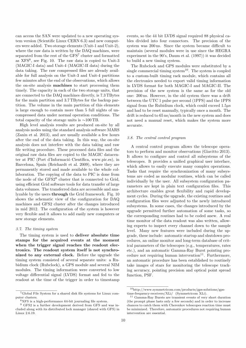
can access the SAN were updated to a new operating sys-tem version (Scientific Linux CERN 6.3) and new comput-ers were added. Two storage elements (Unit-1 and Unit-2),where the raw data is written by the DAQ machines, wereseparated from the rest of the GFS7 cluster and formattedas XFS8, see Fig. 10. The raw data is copied to Unit-3(MAGIC-I data) and Unit-4 (MAGIC-II data) during thedata taking. The raw compressed files are already avail-able for full analysis on the Unit-3 and Unit-4 partitionsfew minutes after the end of the observations, which allowsthe on-site analysis machines to start processing themtimely. The capacity in each of the two storage units, thatare connected to the DAQ machines directly, is 7.3 TBytesfor the main partition and 3.7 TBytes for the backup par-tition. The volume in the main partition of this elementsis large enough to contain more than 5 full nights of un-compressed data under normal operation conditions. Thetotal capacity of the storage units is ∼100 TB.

High level analysis results are produced on-site by allanalysis nodes using the standard analysis software MARS(Zanin et al. 2013), and are usually available a few hoursafter the end of the data taking. In this way, the on-siteanalysis does not interfere with the data taking and rawfile writing procedure. These processed data files and theoriginal raw data files are copied to the MAGIC datacen-ter at PIC (Port d’Informacio Cientıfica, www.pic.es), inBarcelona, Spain (Reichardt et al. 2009), where they arepermanently stored and made available to the whole col-laboration. The copying of the data to PIC is done fromthe node of the GFS29 cluster that is connected to Grid,using efficient Grid software tools for data transfer of largedata volumes. The transferred data are accessible and ana-lyzable by the users through the Grid framework. Fig. 10shows the schematic view of the configuration for DAQmachines and GFS2 cluster after the changes introducedin mid 2012. The configuration of the system is howeververy flexible and it allows to add easily new computers ornew storage elements.

3.7. The timing system

The timing system is used to deliver absolute timestamps for the acquired events at the momentwhen the trigger signal reaches the readout elec-tronics. The readout system itself is not synchro-nized to any external clock. Before the upgrade thetiming system consisted of several separate units: a Ru-bidium clock (Rubclock), a GPS module and several NIMmodules. The timing information were converted to lowvoltage differential signal (LVDS) format and fed to thereadout at the time of the trigger in order to timestamp

7Global File System for a shared disk file systems for Linux com-puter clusters.

8XFS is a high-performance 64-bit journaling file system.9 GFS2 is a further development derived from GFS and was in-

cluded along with its distributed lock manager (shared with GFS) inLinux 2.6.19.

events, so the 44 bit LVDS signal required 88 physical ca-bles divided into four connectors. The precision of thesystem was 200 ns. Since the system became difficult tomaintain (several modules were in use since the HEGRAexperiment in the 90’s, Daum et al. (1997)) it was decidedto build a new timing system.

The Rubclock and GPS modules were substituted by asingle commercial timing system10. The system is coupledto a custom-built timing rack module, which contains allthe electronics needed to export valid timing informationin LVDS format for both MAGIC-I and MAGIC-II. Theprecision of the new system is the same as for the oldone: 200 ns. However, in the old system there was a driftbetween the UTC 1 pulse per second (1PPS) and the 1PPSsignal from the Rubidium clock, which could exceed 1.5µsand had to be reset manually, typically once a month. Thedrift is reduced to 65 ns/month in the new system and doesnot need a manual reset, which makes the system moreaccurate.

3.8. The central control program

A central control program allows the telescope opera-tors to perform and monitor observations (Giavitto 2013).It allows to configure and control all subsystems of thetelescopes. It provides a unified graphical user interface,which allows to easily execute many complex operations.Tasks that require the synchronization of many subsys-tems are coded as modular routines, which can be calledindividually by the user. All subsystem configuration pa-rameters are kept in plain text configuration files. Thisarchitecture enables great flexibility and rapid develop-ment cycles. During the upgrade, the existing routines andconfiguration files were adjusted to the newly introducedsubsystems. In some cases, the changes introduced by theupgrade permitted further automation of some tasks, sothe corresponding routines had to be coded anew. A realtime monitor of the data readout was also written, allow-ing experts to inspect every channel down to the samplelevel. Many new features were included during the up-grade, these include: automatic startup and shutdown pro-cedures, an online monitor and long-term database of crit-ical parameters of the telescopes (e.g., temperatures, ratesetc.), and an automatic Gamma-Ray Burst pointing pro-cedure not requiring human intervention11. Furthermore,an automatic procedure has been established to routinelytake images of stars for monitoring the telescope track-ing accuracy, pointing precision and optical point spreadfunction, PSF.

10http://www.symmetricom.com/products/gps-solutions/gps-time-frequency-receivers/XLi/ (Symmetricom XLi).

11 Gamma-Ray Bursts are transient events of very short duration(the prompt phase lasts only a few seconds) and in order to increasechances to catch them with Cherenkov telescopes reaction time mustbe minimized. Therefore, automatic procedures not requiring humanintervention are essential.

10

UNIT 1 UNIT 2 UNIT 3 UNIT 4

.

Figure 10: Schematic view on the computing network of the DAQ and the data analysis machines in MAGIC.

4. Low level performance

Here we shortly describe the basic performance param-eters of the MAGIC telescope system after the upgrade.

4.1. Sources of noise

The two main sources of noise in the extracted signalsare electronic noise and fluctuations of the night sky back-ground (NSB). The goal of the upgrade was to keep theelectronic noise at a similar level as the noise coming fromthe extragalactic (dark time, no bright stars) NSB. The in-dividual contributions of the noise were extracted by ded-icated runs taken with certain contributions on and offseparately. First only readout electronics was switched onallowing to measure the contribution from the DRS4 andthe receivers. Then the bias current of the camera VC-SELs (see also in Borla-Tridon et al. (2009)) was turnedon, and finally the HV was applied to the PMTs and cam-era opened during night pointing to a dark patch of the sky.The assumption in determining the individual componentsof the electronic noise is that they are mainly independentof each other. The obtained numbers are summarized inTable 2. One can see that the electronics noise (RMS)from the readout is at the level of 0.7 phe, the contribu-tion from the camera (mainly VCSEL for the optical signaltransmission) of 0.3 phe, which is to be compared with thelevel of the NSB of 0.6–0.7 phe. Note that the level of theelectronics noise in phe depends on the target HV used inthe flatfielding procedure (Section 5.2). The applied HVsto the PMTs do not contribute to the noise in any measur-able way. The measured NSB level is higher in MAGIC-IIbecause of newer mirrors that have a higher absolute re-flectivity than the MAGIC-I mirrors (Doro et al. 2008).The relative precision of the measurements is at the level

Source MAGIC-I MAGIC-IIDRS4+receivers 0.76 phe 0.69 phe

VCSEL 0.30 phe 0.30 pheNSB (extragalactic) 0.60 phe 0.72 phe

Total 1.0 phe 1.0 phe

Table 2: Contribution to noise from different hardwarecomponents as well as from the NSB for MAGIC-I pixelsand MAGIC-II (in terms of pedestal RMS).

of a few per cent. The absolute scale of the measurementis about 10%, mainly due to the uncertainties convertingADC counts into phe.

4.2. Linearity in the signal chain

For the linearity of the readout chain we refer to a moredetailed study in Sitarek et al. (2013). The linearity of thefull electronics chain (PMT to the DRS4 readout) is betterthan 10% deviation in the range from 1–2 phe (though it isvery difficult to measure 1 phe signals since the noise levelis of the same order of magnitude) to few hundred phe(see Fig. 11). Some non-linearity of the order of 10-20%is observed for pulses with charge between 200 phe and1000 phe, and signals saturate the readout (at the stageof the receiver board) at >1000 phe. The non-linearityeffect at high charges is mainly due to the behavior of theVCSELs. Simulations showed that a non-linearity of thatmagnitude does not affect image parameters of events witha charge lower than 10,000 phe and has a 1–3% effect forevents with a higher charge, so that no linearity correctionis required.

11

Signal (phe) 1 10 210 310

Non

-line

arity

(%

)

-15

-10

-5

0

5

10

15

Figure 11: Deviation from linearity for 20 typical channelsof the DRS4 readout (Sitarek et al. 2013). The dashedlines mark 1% deviation. A single photoelectron has anamplitude of ∼30 readout counts.

5. Commissioning of the system

The key point of the efficient commissioning was to havea dedicated and well experienced team of 5 to 10 physi-cists at the site of the experiment for a duration of sev-eral months after the installation of the hardware. In thefollowing the main milestones of the commissioning aredescribed.

5.1. Optical point spread function

The optical point spread function (PSF) was improvedduring the upgrade. A dedicated active mirror control(AMC) hardware and software (Biland et al. 2008) takescare of mirror adjustment depending of the zenith angleof observation due to small deformations of the telescopedish. After the new MAGIC-I camera was installed, coun-terweights on the back side of the structure had to bemodified in order to compensate for the heavier weightof the new camera. Once works on the camera and thecounterweights were finished, a new set of look up tables(LUTs) for the AMC were produced to achieve minimaloptical PSF at every zenith angle (no dependence on az-imuth) pointed by the telescope. The LUTs were producedby pointing the telescopes to stars at different zenith an-gles and minimizing the optical PSF (calculated from thereflected image of the star formed on a dedicated mov-able target positioned on the camera plane) by movingthe actuators of the mirror panels. Images of stars aretaken on night by night basis by a special high sensitivityCCD camera (SBIG R©12) located in the center of the dish.A typical on-axis image defining the optical PSF for bothtelescopes is shown in Fig. 12, where the 39% light contain-ment radius is 1.86’ (1.80’) and 95% containment radius

12www.sbig.com

is 7.46’ (6.51’) for the MAGIC-I (MAGIC-II) telescope,respectively. With an increasing angle to the optical axisthe PSF worsens following a second order polynomial func-tion (see Garczarczyk (2006), figure 4.17). Note that theMAGIC camera pixel size has a dimension of 30 mm flat-to-flat of the hexagonal entrance window of the Winstoncone corresponding to a field of view of 6’. The stabilityof the PSF and the absolute reflectivity of the mirrors aresubjects of a forthcoming publication.

5.2. Flatfielding of the PMT gains

Each PMT has a different gain at a fixed HV. The spreadof the gains is unavoidable during the manufacturing pro-cess. We measured such spread in the PMTs for MAGIC Iand found that it is about 30-50% (RMS), depending onthe production line. The signal propagation chain intro-duces further differences in the gain: the optical links aswell as the PIN diodes of the receivers mainly contributeto them. For the purpose of easier calibration of the sig-nals and consistent saturation effects, the HVs applied toPMTs are adjusted such that the resulting signal from cal-ibration pulses (equal photon number at the entrance ofthe PMTs) is equal in readout counts in all pixels whenextracted after the digitization process. The adjustmentof the HVs leads to differences in the transit time of theelectrons in the PMTs. This is taken into account by auto-matically adjusting the delays of the L0 trigger signals (seeSection 5.3). The resulting HV distribution for MAGIC-Iand MAGIC-II cameras can be seen in Fig. 13. The dis-tribution of the MAGIC-I camera is narrower. This is dueto the fact that during the construction of the MAGIC-Icamera the PMTs were divided into two categories, highand low gain ones (see Section 3.1). The high-gain sig-nals are attenuated in the PMT base, which reduces thespread of the resulting gain distribution and consequentlythe spread of the HV distribution. The quality of the HVflatfielding can be seen in Fig. 14, and results very similarfor the two telescopes. During operation, HVs are set onceper night and typically not changed during the night, ex-cept in case of particularly bright light conditions such asstrong moon light13. The RMS (see inlay of the figure) val-ues are similar to the σ of the Gaussian fit (dashed lines),and reach to 2-4% of the corresponding mean value. Thereare two pixels in MAGIC-II that could not be flatfieldedwell because the gain is too low even at the maximum HV.These two pixels can still be used in the analysis, but witha lower signal to noise ratio.

5.3. Trigger adjustments and validation

One of the most relevant systematic uncertainties of thedetector originates from the camera’s inhomogeneous re-sponse to γ rays, starting from how they are triggered.The inhomogeneity of the recorded Cherenkov pulses can

13 We refer to moon phases between the first and the lastquarter.

12

Figure 12: Optical point spread function for the two MAGIC telescopes (MAGIC-I left, MAGIC-II right). The imageof the star called Menkalinan taken with the SBIG R© camera at a zenith distance of 16 degrees.

High Voltage (V)500 600 700 800 900 1000 1100 1200 1300 1400 15000

20

40

60

80

100

120 MAGIC-I

MAGIC-II

Figure 13: Distribution of the high voltages (HVs) appliedto PMTs in MAGIC-I and MAGIC-II cameras after thecharge flatfielding procedure. See text for details. Thehighest voltage that can be applied to the MAGIC PMTsis 1250 V.

come from different gains in the electronic chain, differentelectronic noise levels or different levels of the night skybackground light (presence of stars in the FoV). While therecorded pulses can be calibrated and flatfielded on theanalysis level, the trigger inhomogeneity cannot be eas-ily recovered. Therefore, a special attention is given tomake sure all channels in the trigger are working well, thediscriminator thresholds (DTs) are flatfielded and all mul-tiplicity combinations in the L1 trigger are properly func-

MAGIC-IEntries 1039Mean 7775RMS 209.2

Mean Signal (ADC counts)0 1000 2000 3000 4000 5000 6000 7000 8000 9000

Num

ber

of p

ixel

s

1

10

210

MAGIC-IEntries 1039Mean 7775RMS 209.2

MAGIC-IIEntries 1039Mean 7756RMS 296.9

MAGIC-IIEntries 1039Mean 7756RMS 296.9

Figure 14: Charge distribution of the calibration pulsesin the MAGIC-I (red) and MAGIC-II (blue) cameras afterHV flatfielding. As shown in the statistics, the mean valuesare very similar for the two telescopes whereas the spread(RMS) is 2-4%. Data from 10 October, 2012.

tioning. During the commissioning there were two majortasks concerning the L1 trigger: (a) validation of all nextneighbor multiplicities and (b) the L0 delays are adjustedto assure that the time distribution of the Cherenkov pho-tons in the focal plane of the telescope is conserved at theL1 trigger level, which is achieved by means of referencelight pulses from the calibration box. Dedicated hardware

13

and software have been developed to test all multiplicitiesin short time. The L1 trigger systems of both telescopeshave been extensively tested, hardware mistakes identifiedand repaired.

5.3.1. Evaluation of the L1 trigger

The L1 trigger was evaluated with HYDRA, a multi-thread C-program to test, adjust and monitor the L1 trig-ger. The program is running as a part of the MAGIC Inte-grated Readout (MIR) software, which is the slow controlprogram to steer and monitor individual readout, triggerand calibration system components of the MAGIC tele-scopes (Tescaro et al. 2009). There are many trigger pixelcombinations to test: 1653 for 2NN, 988 for 3NN, 1311 for4NN and 2280 for 5NN. To test the L1 macrocell multi-plicities, signals in all trigger channels are injected. Thiscan be done during the day thanks to the pulse injectionsystem of the camera (see Sec. 3.1). The DTs are set be-low the injected signal for a particular pixel combinationin every macrocell, the others are set high enough to en-sure that they will not trigger. The rate of the macrocellis monitored to identify inoperative combinations. The al-gorithm checks all possible combinations sequentially butit runs in parallel for all 19 macrocells. To go from onecombination to the next one, the DTs must be changed,which takes about 10 ms per pixel. The trigger rate ofthe macrocells is read every 10 ms, which makes the scanfast. The procedure to test all possible trigger combina-tion takes about 15 min allowing for regular monitoringof the trigger performance. During the commissioning ofthe upgraded system, about 20 channels in each telescopewere found not working in the L1 trigger (mostly due toa bad soldering and faulty components), which then wererepaired.

5.3.2. L0 delays and L0 width adjustment

The arrival times of the signals at the L1 logic as wellas the widths of the L0 signals had to be adjusted. Theprecision of the delay and width chips is 10 ps. There is atrade-off between the L1 trigger gate (that depends on thewidths of the L0 signals) and the accuracy of the arrivaltimes adjustment. With no delay adjustment the timespread would have an RMS of 3–4 ns with some outliersup to 10ns. The spread of arrival times is due to differ-ences in transit times of the electrons in PMTs (mainlybecause of different HV applied) and to differences in sig-nal travel time through optical fibers, as well as slightlydifferent response time of electronic components. Finally,in this case not related to the hardware, one also needsto allow for some 2 ns differences in arrival time betweenindividual channels due to the physics of the showers14.Without delay adjustment of individual channels the L1

14The time gradient can be up to 2 ns between neighboring pixelsfor high-energy showers with a large impact distance from the tele-scope. This is a pure physics effect that cannot be tuned/minimizeas the other time differences we discussed in this section.

trigger gate would, therefore, be at least 15 ns to securemaximal efficiency of the L1 coincidence trigger to γ rays.A larger gate corresponds to a higher chance to receivean accidental trigger, and the accidental trigger rate isa factor limiting the energy threshold since discriminatorthresholds have to be increased to keep their rate undercontrol. The goal was, therefore, to keep the gate as low aspossible by adjusting the arrival times between the chan-nels. In the following we describe the approach we used.

In HYDRA, several algorithms were implemented to ad-just the arrival times automatically. Since the transit timein the PMTs has a relevant contribution, the proceduremust be performed with the flatfielded HVs and open cam-era, using calibration pulses (since they arrive simultane-ously at the camera plane, see Section 3.5). The followingalgorithm was chosen to be the standard one: the adjust-ment is done in 3NN logic and a fixed L0 pulse width. Inevery macrocell, the central pixel of the macrocell is con-sidered to be the reference channel. A 2D scan in delaytimes is performed with the two neighboring pixels (in avalid 3NN combination) and the delays are chosen to max-imize the resulting L1 gate. An example of such 2D scansfor 4 different macrocells with a particular 3NN combina-tion between pixels pA, pB and pC is shown in Fig. 15.The delay of pixel pA is kept constant whereas a scan indelays of pixels pB and pC is performed. The axes of theplots indicate pixel delays in ns. The yellow area marksthe delay combinations that result in a valid L1 trigger.The blue cross in the center of the area corresponds to thechosen delays as the result of the scan, and its position isdefined as the crossing point between the maximal inter-vals in both directions (within some tolerances). If thereare several possibilities, the mean values are taken. The re-sulting L1 gates, the maximum width/height of the yellowarea, are in the order of (7 ± 1) ns (Fig. 15). The pro-cedure continues successively over the 3NN combinationsof the macrocell in a spiral by keeping already adjusteddelays fixed. At the end, a cross-calibration procedurebetween the macrocells is applied using the border chan-nels that belong to more than one macrocell. We alsoapply an overall offset to the resulting L0 delays to alignthem at around 5 ns to minimize the trigger latency. Theoverall precision of the adjustment is ±1 ns (RMS). Theprocedure has been tested with different L0 signal widthsfinding that 5.5 ns FWHM is the shortest L0 signal thatgive robust and reproducible results with a high triggerhomogeneity. Although the setting of the delays can notbe done truly in parallel (since the communication bus isserial), the operation is very fast (1µs), so that in prac-tice parallelizing the adjustment for the 19 macrocell givesa factor ∼19 gain in execution time. The HYDRA-basedprocedure to adjust L0 delays (needed every time HVs arechanged) takes about 15 min, which is a substantial im-provement compared to the former manual procedure thatrequired several observing nights to finish. The resultingL0 delays are shown in Fig. 16.

14

Delay pixel B (ns)2 4 6 8 10 12 14 16 18

Del

ay p

ixel

C (

ns)

2468

1012141618

Delay pixel B (ns)2 4 6 8 10 12 14 16 18

Del

ay p

ixel

C (

ns)

2468

1012141618

Delay pixel B (ns)2 4 6 8 10 12 14 16 18

Del

ay p

ixel

C (

ns)

2468

1012141618

Delay pixel B (ns)2 4 6 8 10 12 14 16 18

Del

ay p

ixel

C (

ns)

2468

1012141618

Figure 15: Example of the adjustment of the L0 delaysbetween neighboring pixels of the 3NN logic. Shown are 4macrocells with an example of 3NN combination betweenpixels pA, pB and pC. The result of the scan is shown bythe blue cross. See text for details.

5.3.3. Discriminator threshold (DT) calibration

The goal of the DT calibration is to adjust the DTs ofthe trigger channels (L0 trigger) such that the sensitivityof the channels is flat in terms of photon density ofCherenkov photons. This is achieved by means of a ratescan over the range of DTs for each trigger channel whenfiring calibration light pulses with a given photon density(e.g., equivalent to a mean of 100 photoelectrons (phe)per pixel in the PMTs of the camera). Then, for eachtrigger channel the required DT is determined such that50% of the calibration pulses fulfill the trigger condition.These are the DTs corresponding to a 100 phe level. Wethen scale the DTs linearly to obtain individual pixelthresholds for a desired phe level. The extragalactic darksky15 DTs are set to be at a level of 4.25 phe. For Galacticsources, 15% higher DTs are used. Before the MAGICupgrade, the extragalactic dark sky settings were 4.3 phein MAGIC-I and 5.0 phe in MAGIC-II, respectively(Aleksic et al. 2012). The change in the operation DTsshows that MAGIC-II was improved for operation at alower threshold and MAGIC-I threshold was maintainedconstant despite the larger trigger area. The distributionof the post-upgrade DTs for the two telescopes can beseen in Fig. 17. The spread in the DTs for a homogeneouslight is about ∼15% RMS and is higher than the spread of

15 We define “extragalactic dark sky settings” for an observationoutside the Galactic plane during a dark night. DTs values can bescaled up in case of a FoV inside the Galactic plane or in case ofbrighter light conditions (e.g. with the moon in the sky).

L0 delay (ns)0 1 2 3 4 5 6 7 8 9 10

010

20

30

40

50

60

70

80

90

MAGIC-I

MAGIC-II

Figure 16: Distribution of the L0 trigger delays inMAGIC-I and MAGIC-II after applying the HYDRA op-timization procedure.

the charges (2-4%, see Fig. 14). The reason is that thereare some small differences between the analog (readout)and digital (trigger) signal branches: the signal shapesare not identical, and the DT is applied to the amplitude,whereas the charge is extracted from the integrated signal.

DTs (mV)6 8 10 12 14

0

20

40

60

80

100

120MAGIC-I

MAGIC-II

Figure 17: Distribution of the L0 discriminator thresh-olds (DTs) applied in MAGIC-I and MAGIC-II receiverboards after the charge flatfielding procedure in order toachieve a charge threshold of 4.25 phe.

5.3.4. Individual pixel rate control (IPRC)

During operation, the individual pixel rates (IPRs) aredominated by the night sky background. Bright stars in-side the FoV illuminate small areas of the camera andincrease the IPR of the affected pixels. The flatfieldedDTs may result in very different IPRs during the opera-tion since (a) the response of the PMTs is different for

15

the calibration pulses for which the DTs are calibrated(fixed wavelength 355 nm) and the night sky background(roughly a power law spectrum growing to red wave-lengths) and (b) the rates depend on the sky region thepixel is exposed to (e.g. it may contain stars, which wouldincrease NSB fluctuations and, therefore, the IPR). Dur-ing the commissioning, several algorithms and limits weretested and the following procedure established: As long asthe IPRs are below 1.2 MHz (most of them being in therange of 300–600 kHz), no action is taken. For an IPRoutside of this limit (due to the presence of stars), an IPRcontrol software takes care of increasing the DT for theaffected pixel in order not to spoil the resulting L1 tele-scope rate (the channels are typically still suitable for im-age analysis though). The DT is increased until the pixelrate falls within the limits of 200 kHz – 1.2 MHz. In caseof really bright stars in the pixel FoV (typically with B-magnitude higher than mag 3 causing a DC level higherthan 47µA) the applied HV is automatically reduced toprotect the PMT from fast aging. Once the star is out ofthe FoV of the affected pixel, its IPR will be low becauseof the previously increased DT and once the IPR is below100 kHz the IPR control (IPRC) software resets the DT tothe original value. This procedure ensures a flexibility fordifferent NSB levels and takes care of the stars in the FoVwhile keeping the energy threshold low and most of theDTs flatfielded. It is important to keep the DTs flatfieldedto ensure a good matching between the data and MonteCarlo simulations, where it is assumed that the DTs areidentical for all the pixels. The number of pixels affectedby the procedure depends on the sky field. If it does notcontain many stars with magnitude higher than mag 8there are typically have 1-10 pixels per camera, for whichDTs are modified. For sky fields with many stars we caneasily have up 100-150 affected pixels per camera.

5.3.5. Adjusting the operating point of the trigger

Rate scans have been performed at clear nights at lowzenith angles to determine the trigger rate as a functionof the DTs in phe. Mono (L1) trigger rate scans as well asstereoscopic (L3) trigger rates scans have been performedfor several nights and the performance has been foundto be stable. An example of the rate scans is shown inFig. 18. One can see the steep slope of the rate at low DTs,where the rate is dominated by the chance coincidencedue to NSB and afterpulsing of PMTs. At higher DTs,the trigger rate is dominated by the rate of the cosmicray showers and penetrating muons. One can see thatthe coincidence trigger (L3 trigger) strongly suppressesthe chance coincidence triggers and the triggers due tolocal muons. However, the L3 trigger rate is also lower(the factor is energy dependent) since, for any fixedindividual telescope rate, the stereo collectionarea is smaller than the mono one because it is anintersection of the mono trigger areas of the twotelescopes. For standard operation, the L1 3NN triggerlogic and the hardware stereo (readout of the camera only

Discriminator Threshold (phe)2 4 6 8 10 12 14 16 18 20 22 24

Rat

e (H

z)

10

210

310

410

510

610

710

MAGIC-I L1

MAGIC-II L1

Stereo L3

fit to L3

Figure 18: Rate scans taken by changing discriminatorthresholds (DTs) to optimize the operating point of theMAGIC telescopes. Red (blue) points are L1 3NN ratescans taken with MAGIC-I (MAGIC-II) telescopes and thelines are analytical fits to them. The black points corre-spond to the measured stereoscopic rate of the system, andthe black lines are fitted functions. The operating pointhas been chosen to be 4.25 phe per channel.

for stereo triggers) is used. The operating point for theL0 trigger has been chosen to be 4.25 phe, resulting in astereo rate of around 280 Hz, of which about 40 Hz areaccidental triggers.

When pointing to new observation targets, it takes sev-eral seconds for the IPRC to adjust the DTs to the NSBlight in the FoV. In the commissioning of the system wenoted that, during these short periods, the resulting stereotrigger can be very high (5-100 kHz), being dominated byaccidental triggers. To avoid possible saturation of thedata acquisition with very high trigger rates, which maylead to data corruptions and interruption of data tak-ing procedure, a trigger limiter was installed inside theprescaler16 of each telescope. The trigger limiter evalu-ates the overall trigger rate of a telescope every 10 ms andblocks triggers to the readout for the following 10 ms incase the rate is above a programmable limit. The triggerlimiter is configured to block trigger rates above 1000 Hz.

5.4. DAQ performance

The total acquisition rate that the DAQ has to guar-antee is the sum of the cosmic trigger rate provided bythe L3 trigger (∼280 Hz, see section 5.3.5) plus the contri-bution of the diagnostic calibration and pedestal triggers

16The prescaler board is used in the MAGIC telescope to select thetriggers coming from the individual trigger sources before issuing atrigger signal to the readout system.

16

(25+25 Hz) that are issued interleaved to the physical trig-gers. During the commissioning of the system we adjustedvarious parameters of the DAQ program such as the num-ber of cores used, loads between different threads, DAQbuffer length etc. The total sustainable acquisition of theDAQ system is currently ∼800 Hz (CPU limited, the writ-ing speed being ∼1.1 kHz), more than double than theactual data taking rate.

The CPU overhead is particularly demanding becausebesides the event building, the data integrity check andthe data storage, the DAQ performs two further actions:the DRS4 raw data correction and the extraction of theonline data check values. The raw data correction (see Sec-tion 3.3.3) is a particularly demanding task because it in-volves the manipulation of every single digitized data sam-ple from the readout, that has to be pedestal-subtractedusing the specific single DRS4 capacitor average pedestalvalue (Sitarek et al. 2013).

As discussed in Section 3.3.1, the receiver boards of theupgraded system allow a very precise control of the trig-ger rate even when the light conditions change (IPRC ofthe L0 discriminators). Nevertheless, besides providingthis sustainable average acquisition rate, the DAQ has toguarantee a certain tolerance to sudden increase of the ac-quisition rate17. This capability is guaranteed—withoutevent loss—by the DAQ program design, which relies ona volatile memory ring-buffer bridging the events to thedisk. The event buffer is 10,000 events deep, or 10 s intime at a trigger rate of 1 kHz.

While running, the DAQ also feeds the online analy-sis program dubbed MOLA (see Tescaro et al. 2013, andSection 6).

6. The online analysis client

A real time data analysis is an important part of thesuccess of an IACT experiment. Most of the extragalacticand several Galactic very-high-energy sources are variable,some of them on time scales down to hours and minutes.A real time analysis of the data taken can provide essen-tial time critical internal triggers to extend observation offlaring sources and alert other multiwavelength partners.

The upgraded system allowed to develop a novel pro-gram to fulfill the task of analyzing the data as they arebeing taken (contrary to the on-site analysis mentioned inSection 3.6 that starts when the night is over), and pro-vide online information to the observers of the measuredγ-ray flux and its time evolution: MAGIC Online Analysis(MOLA).

MOLA is a multithreaded C++ program that runs si-multaneously with the data acquisition software and actsas a receiving client of the event informations computed

17Temporary increases of the trigger rate are typically determinedby uncontrolled factors like car-flashes from the astronomers of theobservatory, but might be potentially also due to particularly highγ-ray fluxes from extremely bright flares.

at the very moment the events are acquired by each tele-scope. In fact, as mentioned in the previous section, theDAQ software of MAGIC-I and MAGIC-II computes in-dependently the signal and arrival time of each pixel ofthe telescope cameras. In this way the calculation of theimage parameters and the latest steps of the data analysisare outsourced to a separate program on an independentcomputer.

The multithread program structure consists of threethreads: two reading threads and one analyzing thread.The two reading threads are appointed to receive the datastream via TCP/IP from the two DAQs asynchronouslyand perform the non-stereo analysis steps. The main anal-ysis thread is instead appointed to match the events fromthe two streams and perform the stereoscopic reconstruc-tion (see below).

Two independent TCP/IP streams are activated oncethe program starts, and each time the observation of asource is finished the current results are stored and theanalysis reset. Each event stream contains the pixel signals(integrated charge) and the signal arrival time. The tasksof each reading thread are:

• Receive from the DAQ program, decode and tem-porarily store the relevant information from the eventstream (event tags, charge per pixel and relative ar-rival time).

• Calibrate (flat-field) the gain and identify the deadpixels using interleaved calibration events.

• Check pedestal events to identify and interpolate sig-nals from intrinsically noisy or dead pixels (e.g. pix-els with hardware problems, typically less than 5 percamera).

• Perform image cleaning to select pixels with a signif-icant Cherenkov signal.

• Calculate image parameters, using standard MAGICanalysis software data structures (see Zanin et al.2013).

• Estimate shower direction from a set of relevant pa-rameters (image shape, orientation and time gradientalong the major axis) by means of the RandomForest classification as described in Albert et al.(2008).

Single telescope events have to be combined to formstereo events in order to exploit the full potential of thestereo imaging technique.

The tasks which have to be accomplished in order to ob-tain high level analysis results are performed by the stereoanalysis thread, and can be summarized as follows:

• Identify matching stereo events by means of theunique L3 trigger number.

• Calculate the event direction through a weighted av-erage of the estimates from the two individual images.

17

• Calculate shower core impact point and impact pa-rameters.

• Apply the background suppression by means ofthe hadronness gamma/hadron likelihood parameter(Zanin et al. 2013).

• Apply cuts and compute the signal excess plot withrespect to the candidate source position.

• Produce sky-maps with γ-ray candidate events.

• Produce light curves (time evolution) of the measuredγ-ray flux during the current observations.

Results are produced for two energy ranges: Low Energy(LE) and High Energy (HE) depending of the size of theevent image in phe: The HE sample includes all eventswith at least 125 phe in each of the two telescopes; therest of the events with at least 40 phe in each telescopeconstitutes the LE sample. For Crab Nebula low zenithangles (< 30◦) observations the median energies of thesetwo samples are ∼110 and ∼350 GeV, respectively. In theHE range, the sensitivity of the MOLA analysis at zenithangles below 25◦ zenith angle has been estimated to be1.0% of the Crab Nebula flux in 50 h observation time,which is equivalent to 10% of the Crab Nebula flux in 30minutes.

MOLA provides to the telescope operators high-levelinformation about the currently observed astrophysicalsource such as signal excess plots and sky-maps with γ-raycandidate events, together with diagnostic information re-lated to the signal calibration and the image parameterscalculation. MOLA is commissioned to perform withoutdata loss up to a rate of 600 Hz. For higher data rates(not expected with the current setup), some events will belost for the online analysis but the program will continuerunning with a reduced performance.

7. Conclusions

A major upgrade of the MAGIC telescopes took placein the years 2011–2012. The major items were the instal-lation of the new camera for MAGIC-I, the new trigger inthe MAGIC-I telescope, the upgrade of the readout sys-tem to DRS4 and programmable receiver boards in bothtelescopes. The commissioning of the upgraded systemsuccessfully finished in October 2012, and the telescopesrestarted regular operation. The main goals of the upgradewere an improvement of the sensitivity at low energies,unification of the hardware used, and reduction of downtime due to technical problems. These goals have beensuccessfully achieved, e.g. the down time due to technicalproblems was< 10% of the observation time in the first twoyears after the upgrade was finished, with only less than2% observation time loss due to troubles in the upgradedsubsystems. This is more than a factor of two better thanin the years before the upgrade and at the level required

for the new generation Cherenkov telescopes of the CTAobservatory (Acharya et al. 2013). The expectations con-cerning the sensitivity of MAGIC were conservative sincethey have been surpassed. A comprehensive comparisoncan be found in the Part II of this paper, Aleksic et al.(2014).

8. Acknowledgements

We would like to thank the Instituto de Astrofısicade Canarias for the excellent working conditions at theObservatorio del Roque de los Muchachos in La Palma.The financial support of the German BMBF and MPG,the Italian INFN and INAF, the Swiss National FundSNF, the ERDF under the Spanish MINECO, and theJapanese JSPS and MEXT is gratefully acknowledged.This work was also supported by the Centro de Excelen-cia Severo Ochoa SEV-2012-0234, CPAN CSD2007-00042,and MultiDark CSD2009-00064 projects of the SpanishConsolider-Ingenio 2010 programme, by grant 268740 ofthe Academy of Finland, by the Croatian Science Founda-tion (HrZZ) Project 09/176 and the University of RijekaProject 13.12.1.3.02, by the DFG Collaborative ResearchCenters SFB823/C4 and SFB876/C3, and by the PolishMNiSzW grant 745/N-HESS-MAGIC/2010/0. We thankthe two anonymous referees for thorough reading and help-ful comments on the manuscript.

Acharya, B. S., Actis, M., Aghajani, et al., Mar. 2013. Introducingthe CTA concept. Astroparticle Physics 43, 3–18.

Aharonian, F., Akhperjanian, A. G., Bazer-Bachi, A. R., et al., Oct.2006. Observations of the Crab nebula with HESS. Astronomy &Astrophysics 457, 899–915.

Albert, J., Aliu, E., Anderhub, H., et al., Apr. 2008. Implementa-tion of the Random Forest method for the Imaging AtmosphericCherenkov Telescope MAGIC. Nuclear Instruments and Methodsin Physics Research A 588, 424–432.

Aleksic, J., Alvarez, E. A., Antonelli, L. A., Antoranz, P., Asensio,M., et al., Feb. 2012. Performance of the MAGIC stereo systemobtained with Crab Nebula data. Astroparticle Physics 35, 435–448.

Aleksic, J., Alvarez, E. A., Antonelli, L. A., Antoranz, P., Asensio,M., et al., 2014. The major upgrade of the MAGIC telescopes,Part II: The achieved physics performance using the Crab Nebulaobservations, submitted.

Aliu, E., Anderhub, H., Antonelli, L. A., Antoranz, P., Backes, M.,et al., 2008. Observation of Pulsed Gamma-Rays Above 25 GeVfrom the Crab Pulsar with MAGIC. Science 322, 1221–1224.

Aliu, E., Anderhub, H., Antonelli, L. A., Antoranz, P., Backes, M.,et al., Jan. 2009. Improving the performance of the single-dishCherenkov telescope MAGIC through the use of signal timing.Astroparticle Physics 30, 293–305.

Bartko, H., Goebel, F., Mirzoyan, R., Pimpl, W., Teshima, M., Aug.2005. Tests of a prototype multiplexed fiber-optic ultra-fast FADCdata acquisition system for the MAGIC telescope. Nuclear Instru-ments and Methods in Physics Research A 548, 464–486.

Biland, A., Garczarczyk, M., Anderhub, H., et al., 2008. The ActiveMirror Control of the MAGIC Telescopes. In: 30st ICRC, Merida.Vol. 3 of International Cosmic Ray Conference. pp. 1353–1356.

Bitossi, M., Paoletti, R., Tescaro, D., 2014. Ultra-fast sampling andData Acquisition using the DRS4 Waveform Digitizer, in prepa-ration.

Borla-Tridon, D., Goebel, F., Fink, D., et al., Jul. 2009. Performanceof the Camera of the MAGIC II Telescope. In: 31st ICRC, Lodz.International Cosmic Ray Conference.

18

Carmona, E., Coarasa, J. A., Barcelo, M., for the MAGIC Collab-oration, Jul. 2009. A Flexible High Demand Storage System forMAGIC-I and MAGIC-II using GFS. In: 31st ICRC, Lodz. Inter-national Cosmic Ray Conference.

Daum, A., Hermann, G., Heß, M., et al., Dec. 1997. First resultson the performance of the HEGRA IACT array. AstroparticlePhysics 8, 1–11.

Doro, M., 2012. Reaching the lowest energy threshold of ground-based cherenkov telescopes with magicstereo: A goal achieved.Nuclear Instruments and Methods in Physics Research SectionA: Accelerators, Spectrometers, Detectors and Associated Equip-ment 692 (0), 201 – 207, 3rd Roma International Conference onAstroparticle Physics.

Doro, M., Bastieri, D., Biland, A., Dazzi, F., Font, L., et al., Sep.2008. The reflective surface of the MAGIC telescope. Nuclear In-struments and Methods in Physics Research A 595, 200–203.

Fomin, V. P., Stepanian, A. A., Lamb, R. C., Lewis, D. A., Punch,M., Weekes, T. C., May 1994. New methods of atmosphericCherenkov imaging for gamma-ray astronomy. I. The false sourcemethod. Astroparticle Physics 2, 137–150.

Garczarczyk, M., 2006. First Observations of the GRB Prompt andEarly Afterglow Emission Phase at ∼100 GeV Energy Regimewith the 17m Diameter MAGIC Imaging Atmospheric CherenkovTelescope. Ph.D. thesis, University of Rostock, Germany,https://magicold.mpp.mpg.de/publications/theses/MGarczarczyk.pdf.

Giavitto, G., 2013. Observing the VHE Gamma-Ray Sky with theMAGIC Telescopes: the Blazar B3 2247+381 and the Crab Pulsar.

Hillas, A. M., Aug. 1985. Cerenkov light images of EAS producedby primary gamma. International Cosmic Ray Conference 3, 445–448.

Hinton, J., 2009. Ground-based gamma-ray astronomy withCherenkov telescopes. New J. Phys. 11, 055005.

Holder, J., Acciari, V. A., Aliu, E., et al., Dec. 2008. Status ofthe VERITAS Observatory. In: Aharonian, F. A., Hofmann, W.,Rieger, F. (Eds.), American Institute of Physics Conference Se-ries. Vol. 1085 of American Institute of Physics Conference Series.pp. 657–660.

Lorenz, E., Apr. 2004. Status of the 17 m MAGIC telescope. NewA Rev.48, 339–344.

Lorenz, E., Wagner, R., Aug. 2012. Very-high energy gamma-rayastronomy. A 23-year success story in high-energy astroparticlephysics. European Physical Journal H 37, 459–513.

Mirzoyan, R., Lorenz, E., 1997. On the Calibration Accuracy of LightSensors in Atmospheric Cherenkov Fluorescence and Neutrino Ex-periments. International Cosmic Ray Conference 7, 265.

Reichardt, I., Rico, J., Carmona, E., et al., Jul. 2009. The MAGICData Center. In: 31st ICRC, Lodz. International Cosmic Ray Con-ference.

Rodriguez Garcia, J., et al., 2013. Status of the new Sum-Triggersystem for the MAGIC telescopes. In: 33rd ICRC, Rio De Janeiro.International Cosmic Ray Conference.

Schweizer, T., Lorenz, E., Martinez, M., Ostankov, A., Paneque,D., Oct. 2002. The optical calibration of the MAGIC telescopecamera. IEEE Transactions on Nuclear Science 49, 2497–2503.

Sitarek, J., Gaug, M., Mazin, D., Paoletti, R., Tescaro, D., Sep. 2013.Analysis techniques and performance of the Domino Ring Sam-pler version 4 based readout for the MAGIC telescopes. NuclearInstruments and Methods in Physics Research A 723, 109–120.

Tescaro, D., Aleksic, J., Barcelo, M., Bitossi, M., Cortina, J., Fras,M., Hadasch, D., Illa, J. M., Martinez, M., Mazin, D., Paoletti, R.,Pegna, R., for the MAGIC Collaboration, Jul. 2009. The readoutsystem of the MAGIC-II Cherenkov Telescope. In: 31st ICRC,Lodz. International Cosmic Ray Conference.

Tescaro, D., Lopez-Oramas, A., Moralejo, A., Mazin, D., DanielaHadasch for the MAGIC Collaboration, Oct. 2013. The MAGICtelescopes DAQ software and the on-the-fly online analysis client.In: 33rd ICRC, Rio De Janeiro. International Cosmic Ray Con-ference.

Zanin, R., et al., 2013. MARS, the MAGIC analysis and reconstruc-tion software. In: International Cosmic Ray Conference. Interna-tional Cosmic Ray Conference.

19