The Leverage Cycle

John Geanakoplos

April 9, 2009

Abstract

Equilibrium determines leverage, not just interest rates. Variations in lever-age cause wild fluctuations in asset prices. This leverage cycle can be damagingto the economy, and should be regulated.

1 Introduction to the Leverage Cycle

At least since the time of Irving Fisher, economists, as well as the general public, haveregarded the interest rate as the most important variable in the economy. But in timesof crisis, collateral rates (equivalently margins or leverage) are far more important.Despite the cries of newspapers to lower the interest rates, the Fed would sometimesdo much better to attend to the economy-wide leverage and leave the interest ratealone. The Fed ought to rethink its priorities.When a homeowner (or hedge fund or a big investment bank) takes out a loan

using say a house as collateral, he must negotiate not just the interest rate, but howmuch he can borrow. If the house costs $100 and he borrows $80 and pays $20 incash, we say that the margin or haircut is 20%, and the loan to value is $80/$100 =80%. The leverage is the reciprocal of the margin, namely the ratio of the asset valueto the cash needed to purchase it, or $100/$20 = 5.In standard economic theory, the equilibrium of supply and demand determines

the interest rate on loans. It would seem impossible that one equation could determinetwo variables, the interest rate and the margin. But in my theory, supply and demanddo determine both the equilibrium leverage (or margin) and the interest rate.It is apparent from everyday life that the laws of supply and demand can determine

both the interest rate and leverage of a loan: the more impatient borrowers are,the higher the interest rate; the more nervous the lenders become, the higher thecollateral they demand. But standard economic theory fails to properly capture theseeffects, struggling to see how a single supply-equals-demand equation for a loan coulddetermine two variables: the interest rate and the leverage. The theory typicallyignores the possibility of default (and thus the need for collateral), or else fixes theleverage as a constant, allowing the equation to predict the interest rate.

1

Yet variation in leverage has a huge impact on the price of assets, contributing toeconomic bubbles and busts. This is because for many assets there is a class of buyerfor whom the asset is more valuable than it is for the rest of the public (standard eco-nomic theory, in contrast, assumes that asset prices reflect some fundamental value).These buyers are willing to pay more, perhaps because they are more sophisticatedand know better how to hedge their exposure to the assets, or they are more risktol-erant, or they simply like the assets more. If they can get their hands on more moneythrough more highly leveraged borrowing (that is, getting a loan with less collateral),they will spend it on the assets and drive those prices up. If they lose wealth, or losethe ability to borrow, they will buy less, so the asset will fall into more pessimistichands and be valued less.In the absence of intervention, leverage becomes too high in boom times, and too

low in bad times. As a result, in boom times asset prices are too high, and in crisistimes they are too low. This is the leverage cycle.Leverage dramatically increased in the United States from 1999 to 2006. A bank

that in 2006 wanted to buy a AAA-rated mortgage security could borrow 98.4% ofthe purchase price, using the security as collateral, and pay only 1.6% in cash. Theleverage was thus 100 to 1.6, or about 60 to 1. The average leverage in 2006 acrossall of the US$2.5 trillion of so-called ‘toxic’ mortgage securities was about 16 to 1,meaning that the buyers paid down only $150 billion and borrowed the other $2.35trillion. Home buyers could get a mortgage leveraged 20 to 1, a 5% down payment.Security and house prices soared.Today leverage has been drastically curtailed by nervous lenders wanting more

collateral for every dollar loaned. Those toxic mortgage securities are now leveragedon average only about 1.5 to 1. Home buyers can now only leverage themselves 5 to 1if they can get a government loan, and less if they need a private loan. De-leveragingis the main reason the prices of both securities and homes are still falling.The leverage cycle is a recurring phenomenon. The financial derivatives crisis

in 1994 that bankrupted Orange County in California was the tail end of a lever-age cycle. So was the emerging markets mortgage crisis of 1998, which brought theConnecticut-based hedge fund Long-Term Capital Management to its knees, prompt-ing an emergency rescue by other financial institutions.In ebullient times competition drives leverage higher and higher. An investor

comes to a hedge fund and says the fund down the block is getting higher returns.The fund manager says the other guy is just leveraging more. The investor responds,well whatever he’s doing, he’s getting higher returns. Pretty soon both funds areleveraging more. During a crisis, leverage can fall by 50% overnight, and by moreover a few days or months. A homeowner who bought his house last year by taking outa subprime mortgage with only 5% down cannot take out a similar loan today withoutputting down 25% (unless he qualifies for one of the government rescue programs).The odds are great that he wouldn’t have the cash to do it, and reducing the interestrate by 1 or 2% won’t change his ability to act.

2

The policy implication of my theory of equilibrium leverage is that the fed shouldmanage system wide leverage, curtailing leverage in normal or ebullient times, andpropping up leverage in anxious times.I fully agree that if agents extrapolate blindly, assuming from past rising prices

that they can safely set very small margin requirements, or that falling prices meansthat it is necessary to demand absurd collateral levels, then the cycle will get muchworse. But a crucial part of my leverage cycle story is that every agent is actingperfectly rationally from his own individual point of view. People are not deceivedinto following illusory trends. They do not ignore danger signs. They do not panic.They look forward, not backward. But under certain circumstances the cycle spiralsinto a crash anyway. The lesson is that even if people remember this leverage cycle,there will be more leverage cycles in the future, unless the Fed acts to stop them.The crash always involves the same three elements. First is scary bad news that

increases uncertainty. This leads to tighter margins as lenders get more nervous.This in turn leads to falling prices and huge losses by the most optimistic, leveragedbuyers. All three elements feed back on each other; the redistribution of wealth fromoptimists to pessimists further erodes prices, causing more losses for optimists, andsteeper price declines, which rational lenders anticipate, leading then to demand morecollateral, and so on.The best way to stop a crash is to prevent it from happening in the first place, by

restricting leverage in ebullient times.To reverse the crash once it has happened requires reversing the three causes. In

today’s environment, that means stopping foreclosures and the free fall of housingprices. As we shall see, the only reliable way to do that is to write down principal.Second, leverage must be restored to sane, intermediate levels. The fed must steparound the banks and lend directly to investors, at more generous collateral levelsthan the private markets are willling to provide. And third, the Treasury must injectoptimistic capital to make up for the lost buying power of the bankrupt leveragedoptimists. This might also entail bailing out various crucial players.My theory is of course not completely original. Over 400 years ago Shakespeare

explained that to take out a loan one had to negotiate both the interest rate andthe collateral level. It is clear which of the two Shakespeare thought was the moreimportant. Who can remember the interest rate Shylock charged Antonio? Buteverybody remembers the pound of flesh that Shylock and Antonio agreed on ascollateral. The upshot of the play, moreover, is that the regulatory authority (thecourt) decides that the collateral level Shylock and Antonio agreed upon was sociallysuboptimal, and the court decrees a different collateral level. The Fed too shouldsometimes decree different collateral levels.In more recent times there has been pioneering work on collateral by Bernanke,

Gertler, Gilchrist, Kiyotaki and Moore. This work emphasized the feedback fromthe fall in collateral prices to a fall in borrowing capacity, assuming a constant loanto value ratio. By contrast, my work defining collateral equilibrium, which was first

3

published in 1997, contemporaneously with Kiyotaki and Moore, focused on whatdetermines the ratios (LTV, margin, or leverage) and why they change. In practice, Ibelieve the change in ratios has been far bigger and more important than the changein levels. In 2003 I published my leverage cycle theory on the anatomy of crashes andmargins (it was an invited address at the 2002 World Econometric Society meetings),arguing that in normal times leverage gets too high, and in bad times leverage istoo low. In 2008 I published a paper in the AER with Ana Fostel on leverage cyclesand the anxious economy. There we noted that margins do not move in lock stepacross asset classes, ad that a leverage cycle in one asset class might spread to otherunrelated asset classes. In a paper with Bill Zame we describe the general propertiesof collateral equilibrium. In joint work with Felix Kubler, we show that managingcollateral levels can lead to pareto improvements.

1.1 Survey of Literature

In addition to previously mentioned articles, must mention Minsky moments, Kindle-berger, Tobin on collateral, and more recently, Brunnermeier and Pedersen, Shin,Allen and Gale, Banerjee, Shleifer and Vishny.

1.2 Why was this leverage cycle worse than previous cycles?

There are a number of elements that played into the leverage cycle crisis of 2007-9that had not appeared before, which explain why it has been so bad. I will graduallyincorporate them into the model. The first I have already mentioned, namely thatleverage got higher than ever before.The second is the invention of the credit default swap. The buyer of "CDS insur-

ance" gets a dollar for every dollar of defaulted principal on some bond. But he isnot limited to buying as much insurance as he owns bonds. In fact, he very likely isbuying the CDS nowadays because he thinks the bonds are bad and does not wantto own them at all. CDS are, despite their names, not insurance at all, but a vehiclefor pessimists to leverage their views. Conventional leverage allows optimists to pushthe price of assets unduly high; CDS allows pessimists to push asset prices undulylow. The standardization of CDS for mortgages in late 2005 led to their trades inlarge quantities in 2006 and 2007. This I believe was one of the precipitators of thedownturn.Third, this leverage cycle was really a combination of two leverage cyles, in

mortage securities and in housing. The two reinforce each other. The tighteningmargins in securities led to lower security prices, which made it harder to issue newmortgages, which made it harder for homeowners to refinance, which made themmore likely to default, which made securities riskier, which made their margins gettighter and so on.Fourth, and perhaps most important, when promises exceed collateral values, as

4

when housing is "under water" or upside down", there are typically large losses inturning over the collateral. Today subprime bondholders expect only 25% of the loanamount back when they foreclose on a home. A huge number of homes are expectedto be foreclosed (some say 8 million). The point will be that even if borrowers andlenders foresee that the loan amount is so large then there will be states in which thecollateral is under water, and therefore will cause deadweight losses, they will not beable to prevent themselves from agreeing on such levels.Fifth, the leverage cycle potentially has a major impact on productive activities.

High asset prices means strong incentives for production, and a boon to real con-struction. The fall in asset prices has a blighting effect on new real activity. This isthe essence of Tobin’s Q. And it is the real reason why the crisis stage of the leveragecycle is so alarming.

1.3 Outline

I present the basic model of the leverage cycle drawing on my 2003 paper, in whicha continuum of investors vary in their optimism. I explain how equilibrium candetermine a unique leverage ratio, and I show how dynamic variations in equilibriumleverage arise from changing conditions, and in turn produce dramatic effects on assetprices. This is a context in which the leverage cycle is very easy to see. The welfareimplications, on the other hand, do not seem so dire, because with complete marketsone would also see large fluctuations in asset prices. I therefore move to a secondmodel, drawn from my 1997 paper, in which probabilities are objectively given, andheterogeneity arises from differences in the utility for housing. Once again leverageis endogenously determined, but now the asset prices are much more volatile thanthey would be with complete markets, and the welfare situation is very different(though not necessarily Pareto worse). Along the way I add the particular elementsmentioned above that explain why this cycle was so bad. The last section combinesthe two previous approaches to explain the double leverage cycle, in housing and insecurities, which is an essential element of our current crisis.

1.4 Crises

Crises do not really occur just from coordination failures. There are no self confirmingruns on the bank without some bad news. But not all bad news lead to crises, evenwhen the news is very bad.Bad news in my view must be of a special kind to cause an adverse move in the

leverage cycle. The special bad news must not only lower expectations (as by defini-tion all bad news does), but it must create more uncertainty, and more disagreement.On average news reduces uncertainty, so I have in mind a special, but by no meansunusual, kind of news. The idea is that at the beginning, everyone thinks the chancesof ultimate failure require too many things to go wrong to be of any substantial prob-

5

ability. There is little uncertainty, and therefore little room for disagreement. Onceenough things go wrong to raise the spectre of real trouble, the uncertainty goes wayup in everyone’s mind, and so does the possibility of disagreement.An example occurs when output is 1 unless two things go wrong, in which case

output becomes .2. If an optimist thinks the chance of each thing going wrong isindependent and equal to .1, then it is easy to see that he thinks the chance ofultimate breakdown is .01=(.1)(.1). Expected output for him is .992. In his view exante, the variance of final output is .99(.01)(1−.2) = .0079. After the first piece of badnew, his expected output drops to .92. But the variance jumps to .9(.1)(1−.2) = .072,a tenfold increase.A pessimist who believes the probability of each piece of bad news is independent

and equal to .5 originally thinks the probability of ultimate breakdown is .25=(.5)(.5).Expected output for him is .85. In his view ex ante, the variance of final output is.75(.25)(1− .2) = .15. After the first piece of bad new, his expected output drops to.6. But the variance jumps to .5(.5)(1− .2) = .20. Note that the expectations differedoriginally by .992 − .85 = .142, but after the bad news the disagreement more thandoubles to .92− .6 = .32.I call the kind of bad news that increases uncertainty and disagreement scary

news.The news in the last 18 months has indeed been of this kind. When agency

mortgage default losses were less than 1/4%, there was not much uncertainty andnot much disagreement. Even if they tripled, they would still be small enough notto matter. Similarly, when subprime mortgage losses (that is losses incurred afterhomeowners failed to pay, were thrown out of their homes, and the house was soldfor less than the loan amount) 3%, they were so far under the bond cushion of 8%that there was not much uncertainty or disagreement about whether the bonds wouldsuffer losses, especially the higher rated bonds (with cushions of 15% or more).

1.5 Anatomy of a Crash

I use my theory of the equilibrium leverage to outline the anatomy of market crashesafter the kind of scary news I just described.i) Assets go down in value on scary bad news.ii) This causes a big drop in the wealth of the natural buyers (optimists) who were

leveraged.iii) This leads to further loss in asset value, and in wealth for the natural buyers.iv) Then margin requirements are tightened because of increased uncertainty and

disagreement.v) This causes huge losses in asset values via forced sales.vi) Many optimists will lose all their wealth and go out of businessvii) There may be spillovers if sales of other assets are forced.viii) Investors who survive have a great opportunity.

6

1.6 Natural Buyers

A crucial part of my story is heterogeneity between investors. The natural buyers wantthe asset more than the general public. This could be for many reasons. The naturalbuyers could be less risk averse. Or they could have access to hedging techniques thegeneral public does not that make the assets less dangerous for them. Or they couldget more utility out of holding the assets. Or they could have access to a productiontechnology that uses the assets more efficiently than the general public. Or theycould have special information based on local knowledge. Or they could simply bemore optimistic. I have tried nearly all these possibilities at various times in mymodels. In the real world, the natural buyers are probably made up of a mixture ofthese categories. But for modeling purposes, the simplest is the last, namely thatthe natural buyers are more optimistic by nature. They have different priors fromthe pessimists. I note simply that this perspective is not really so different fromthe others. Differences in risk aversion in the end just mean different risk adjustedprobabilities.A crucial part of the story then is the heterogeneity between optimists and pes-

simists. A loss for the optimists is much more important to prices than a loss forthe pessimists, because it is the optimists who will be holding the assets and biddingtheir prices up. The loss of access to capital by the optimists (and the subsequentmoving of assets from optimists to pessimists) creates the crash.Current events have certainly borne out this heterogeneity hypothesis. When

the big banks (who are the classic natural buyers) lost lots of capital through theirblunders in the CDOmarket, that had a profound effect on new investments. Some ofthat capital was restored by international investments from Singapore and so on, butit was not enough, and it quickly dried up when the initial investments lost money.Macroeconomists have often ignored the natural buyers hypothesis. For example,

some macroeconomists compute the marginal propensity to consume out of wealth,and find it very low. The loss of $250 billion dollars of wealth could not possiblymatter much they said, because the stock market has fallen many times by muchmore and economic activity hardly changed. But that ignores who lost the money.The natural buyers hypothesis is not original with me. The innovation is in

combining it with equilibrium leverage.I do not presume a cut and dried distinction between natural buyers and the

public. I imagine a continuum of agents uniformly arrayed between 0 and 1. Agent hon that continuum thinks the probability of good news is g(h) = h, and the probabilityof bad news is b(h) = 1− h. The higher the h, the more optimistic the agent.The more optimistic an agent, the more natural a buyer he is. By having a

continuum I avoid a rigid categorization of agents. The agents will choose whether tobe borrowers and buyers of risky assets, or lenders and sellers of risky assets. Therewill be some break point h* such that those more optimistic than h∗, h > h∗, are onone side of the market and and those with h < h∗ are on the others side. But thisbreak will be endogenous, depending on the exact circumstances.

7

Natural buyers

public

Natural Buyers-Margins Theory of Crashes

h=0

h=1

2 Borrowing and Asset Pricing

Consider a simple example with one consumption good C, and one asset Y , thatcan pay either 1 or .2 per unit. Imagine the asset as a mortgage that either paysin full or defaults with recovery .2. But it could also be an oil well that might be agusher or small. Or a house with good or bad resale value next period. Let everyagent own one unit of the asset at time 0 and also one unit of the consumptiongood at time 0. For simplicity we think of the consumption good as something thatcan be used immediately in a quantity c that is chosen, or costlessly warehoused(stored) in a quantity denoted by w, like oil or cigarettes or canned food or simplygold (that can be used as fillings) or money. The agents only care about the totalexpected consumption they get, no matter when they get it. They are not impatient.The difference between the agents is only in the probability each attaches to a goodoutcome vs default. (All mortgages will either default together or pay off together). Iimagine the agents arranged uniformly on a continuum, with agent h ∈ [0, 1] assigningprobability h to the good outcomeSee diagram 1.More formally, denoting the amount of consumption C in state s of by cs, and the

holding in state s of Y by ys, and the storage of the consumption good at time 0 by

8

Let each agent h ∈ H ⊂ [0,1]assign probability h to s = Uand probability 1 − h to s = D. Agents with h near 1 are optimists, agents with h near 0are pessimists.

Endogenous Collateral with Heterogeneous Beliefs: A Simple Example

Suppose that 1 unit of Y gives $1 unit in state U and .2 units in D.

U

D

Y=.2

0

h

1 – h

Figure 2

Y=1

w0 we have

uh(c0, y0, w0, cU , cD) = c0 + hcU + (1− h)cD

eh = (ehCo, ehYo , e

hCU, ehCD) = (1, 1, 0, 0)

Storing goods and holding assets provide no direct utility, they just increase incomein the future.Suppose the price of the asset per unit at time 0 is p, somewhere between 0 and

1. The agents h who believe that

h1 + (1− h).2 > p

will want to buy the asset, since by paying p now they get something with expectedpayoff next period greater than p and they are not impatient. Those who think

h1 + (1− h).2 < p

will want to sell their share of the asset. I suppose there is no short selling, but I allowfor borrowing. In the real world it is impossible to short sell many assets other thanstocks. Even when it is possible, only a few agents know how, and those typically arethe optimistic agents who are most likely to want to buy. So the assumption of noshort selling is quite realistic.

9

If borrowing were not allowed, then the asset would have to be held by a largepart of the population. The price of the asset would be .68. Agent h = .60 valuesthe asset at .68 = .60(1) + .40(.2). So all those h below .60 will sell all they have, or.60(1) = .60 in aggregate. Every agent above .60 will buy as much as he can afford.Each of these agents has just enough wealth to buy 1/.68 ≈ 1.5 more units, hence.40(1.5) = .60 units in aggregate. Since the market for assets clears at time 0, this isthe equilibrium with no borrowing.More formally, taking the price of the consumption good in each period to be 1

and the price of Y to be p, we can write the budget set without borrowing for eachagent as

BhN(p) = {(c0, y0, w0, c1, c2) ∈ R5+ : c0 + w0 + p(y0 − 1) = 1cU = w0 + y0

cD = w0 + (.2)y0}.

Given the price p, each agent chooses the consumption plan (ch0 , yh0 , w

h0 , c

h1 , c

h2) in

BhN(p) that maximizes his utility uh defined above. In equilibrium all markets mustclear Z 1

0

(ch0 + wh0 )dh = 1Z 1

0

yh0dh = 1Z 1

0

chUdh = 1 +

Z 1

0

wh0dhZ 1

0

chDdh = .2 +

Z 1

0

wh0dh

In this equilibrium agents are indifferent to storing or consuming right away, so wecan describe equilibrium as if everyone warehoused and postponed consumption bytaking

p = .68

(ch0 , yh0 , w

h0 , c

h1 , c

h2) = (0, 2.5, 0, 2.5, .5) for h ≥ .60

(ch0 , yh0 , w

h0 , c

hU , c

hD) = (0, 0, 1.68, 1.68, 1.68) for h < .60.

When loan markets are created, a smaller group of less than 40% of the agents willbe able to buy and hold the entire stock of the asset. If borrowing were unlimited, atan interest rate of 0, the single agent at the top would borrow so much that he wouldbuy up all the assets by himself. And then the price of the asset would be 1, since atany price p lower than 1 the agents h just below 1 would snatch the asset away fromh = 1. But this agent would default, and so the interest rate would not be zero, andthe equilibrium allocation needs to be more delicately calculated.

10

2.1 Incomplete Markets

We shall restrict attention to loans that are non-contingent, that is that involvepromises of the same amount ϕ in both states. It is evident that the equilibriumallocation under this restriction will in general not be Pareto efficient. For example,in the no borrowing equilibrium, everyone would gain from the transfer of ε > 0 unitsof consumption in state U from each h < .60 to each agent with h > .60, and thetransfer of 3ε/2 units of consumption in state D from each h > .60 to each agent withh < .60. The reason this has not been done in the equilibrium is that there is no assetthat can be traded that moves money from U to D or vice versa. We say that theasset markets are incomplete. We shall assume this incompleteness for a long time,until we consider Credit Default Swaps.

2.2 Collateral

We have not yet determined how much people can borrow or lend. In conventionaleconomics they can do as much of either as they like, at the going interest rate. But inreal life lenders worry about default. Suppose we imagine that the only way to enforcedeliveries is through collateral. A borrower can use the asset itself as collateral, sothat if he defaults the collateral can be seized. Of course a lender realizes that if thepromise is ϕ in both states, then he will only receive

min(ϕ, 1) if good news

min(ϕ, .2) if bad news

The introduction of collateralized loan markets introduces two more parameters: howmuch can be promised ϕ, and at what interest rate r?Suppose that borrowing were arbitrarily limited to ϕ ≤ .2 per unit of Y, that is

suppose agents were allowed to promise at most .2 units of consumption per unit ofthe collateral Y they put up. That is a natural limit, since it is the biggest promisethat is sure to be covered by the collateral. It also greatly simplifies our notation,because then there would be no need to worry about default.Borrowing gives the most optimistic agents a chance to spend more. And this will

push up the price of the asset. But since they can borrow strictly less than the valueof the collateral, optimistic spending will still be limited. Each time an agent buys ahouse, he has to put some of his own money down in addition to the loan amount hecan obtain from the collateral just purchased. He will eventually run out of capital.We can describe the budget set formally with our extra variables.

Bh.2(p, r) = {(c0, y0, ϕ0, w0, c1, c2) ∈ R6+ :

c0 + w0 + p(y0 − 1) = 1 +1

1 + rϕ0 : ϕ0 ≤ .2

cU = w0 + y0 − ϕ0

cD = w0 + (.2)y0 − ϕ0}.

11

Note that ϕ0 > 0 means that the agent is making promises in order to borrowmoney to spend more at time 0. Similarly, ϕ0 < 0 means the agent is buying promiseswhich will reduce his expenditures on consumption and assets in period 0, but enablehim to consume more in the future states U and D. Equilibrium is defined by theprice and interest rate (p, r) and agent choices (ch0 , y

h0 , ϕ

h0 , w

h0 , c

hU , c

hD) in B

h.2(p, r) that

maximizes his utility uh defined above. In equilibrium all markets must clearZ 1

0

(ch0 + wh0 )dh = 1Z 1

0

yh0dh = 1Z 1

0

ϕh0dh = 0Z 1

0

chUdh = 1 +

Z 1

0

wh0dhZ 1

0

chDdh = .2 +

Z 1

0

wh0dh

Clearly the no borrowing equilibrium is a special case of the collateral equilibrium,once the limit .2 on promises is replaced by 0.One can calculate that the equilibrium price of the asset is now .75. At that price

agent h = .69 is just indifferent to buying. Those h < .69 will sell all they have, andthose h > .69 will buy all they can with their cash and with the money they canborrow. One can check that the top 31% of agents will indeed demand exactly whatthe bottom 69% are selling.Who would be doing the borrowing and lending? The top 31% is borrowing to

the max, in order to get their hands on what they believe are cheap assetss. Thebottom 69% do not need the money for buying the asset, so they are willing to lendit. And what interest rate would they get? 0% interest, because they are not lendingall they have in cash. (Their total lending is in fact .2/.69 = .29 < 1 per person).Since they are not impatient and they have plenty of cash left, they are indifferent tolending at 0%. Competition among these lenders will drive the interest rate to 0%.More formally, we can define the equilibrium equations as

p = h∗1 + (1− h∗)(.2)

p =(1− h∗)(1) + .2

h∗

The first equation says that the marginal buyer h∗ is indifferent to buying theasset. The second equation says that the price of Y is equal to the amount of moneythe agents above h∗ spend buying it, divided by the amount of the asset sold. Thenumerator is then all the top group’s consumption endowment, (1− h∗)(1), plus all

12

they can borrow after they get their hands on all of Y, namely .2/(1 + r) = .2. Thedenominator is comprised of all the sales of one unit of Y each by the agents belowh∗.We must also take into account buying on margin. An agent who buys the asset

while simultaneously selling as many promises as he can will only have to pay downp− .2. His return will be nothing in the down state, because then he will have to turnover all the collateral to pay back his loan. But in the up state he will make a profitof 1 − .2. So we need a third equation that says that agent h∗ is indifferent to notbuying the asset or buying the asset on margin.

p− .2 = h∗(1− .2)

But this equation is automatically satisfied as long as p is set to satisfy the firstequation above; simply subtract .2 from both sides. When an agent has constantmarginal utility for consumption, he will be indifferent to buying outright and buyingon margin. In a later section we shall see that when agents have diminishing marginalutility for consumption, they will strictly prefer to buy on margin.As we said, the large supply of durable consumption good, no impatience, and no

default implies that the equilibrium interest rate must be 0. Solving the two equationsabove and plugging these into the agent optimization gives equilibrium

h∗ = .69

(p, r) = (.75, 0),

(ch0 , yh0 , ϕ

h0 , w

h0 , c

h1 , c

h2) = (0, 3.2, .64, 0, 2.6, 0) for h ≥ .69

(ch0 , yh0 , ϕ

h0 , w

h0 , c

h1 , c

h2) = (0, 0,−.3, 1.45, 1.75, 1.75) for h < .69.

Notice that the price rises modestly, because there is a modest amount of bor-rowing. Notice also that even at the higher price, fewer agents hold all the assets(because they can afford to buy on borrowed money).The lesson here is that the looser the collateral requirement, the higher will be

the prices of assets. This has not been properly understood by economists. Theconventional view is that the lower is the interest rate, then the higher will assetprices be, because their cash flows will be discounted less. But in the example I justdescribed, where agents are patient, the interest rate will be zero regardless of thelending (up to some huge amount). The fundamentals do not change, but because of achange in lending standards, asset prices rise. Clearly there is something wrong withconventional asset pricing formulas. The problem is that to compute fundamentalvalue, one has to use probablities. But whose probabilities?The recent run up in asset prices has been attributed to irrational exuberance

because conventional pricing formulas based on fundamental values failed to explainit. But the explanation I propose is that it got easier and easier to borrow. We shallreturn to this momentarily, after we figure out how much people can borrow.

13

Before turning to the next section, observe that equilibrium leverage is

.75

(.75− .2)= 1.4.

The loan to value is .2/.75 = 27%, the margin or haircut was .55/.75 = 73%. In theno borrowing equilibrium, leverage was obviously 1.But leverage cannot yet be said to be endogenous, since we have exogenously fixed

the collateral level or maximal promise at .2. Why wouldn’t the most optimistic buy-ers be willing to borrow more, defaulting in the bad state of course, but compensatingthe lenders by paying a higher interest rate?

2.3 Equilibrium Leverage

Any lender must balance what he foresees getting repaid against the loan amount hegives up at time 0.So how much can an agent borrow at time 0 using one asset worth p as collateral?

In the example where promises were restricted to $2, agents (at the prevailing interestrate of 0) borrowed $2.But why should haircuts be so high? Or equivalently, why should leverage be so

low?Before 1997 there had been virtually no work on equilibrium margins. Collateral

was discussed almost exclusively in models without uncertainty. Even now the fewwriters who try to make collateral endogenous do so by taking an ad hoc measureof risk, like volatility or value at risk, and assume that the margin is some arbitraryfunction of the riskiness of the repayment.It is not surprising that economists have had trouble modeling equilibrium haircuts

or leverage. We have been taught that the only equilibrating variables are prices. Itseems impossible that the demand equals supply equation for loans could determinetwo variables.The key is to think of many loans, not one loan. Irving Fisher and then Ken

Arrow taught us to index commodities by their location, or their time period, or bythe state of nature, so that the same quality apple in different places or differentperiods might have different prices. So we must index each promise by its collateral.A promise of .2 backed by a house is different from a promise of .2 backed by 2/3 ofa house. The former will deliver .2 in both states, but the latter will deliver .2 in thegood state and only 1.33 in the bad state. The collateral matters.Conceptually we must replace the notion of contracts as promises with the notion

of contracts as ordered pairs of promises and collateral. Each ordered pair-contractwill trade in a separate market, with its own price.

Contractj = (Pr omisej, Collateralj) = (Aj, Cj)

The ordered pairs are homogeneous of degree one. A promise of .2 backed by 2/3of a house is simply 2/3 of a promise of .3 backed by a full house. So without loss of

14

generality, we can always normalize the collateral. In our example we shall focus oncontracts in which the collateral Cj is simply one unit of Y.So let us denote by j the promise of j in both states in the future, backed by

the collateral of one unit of Y. We take an arbitrarily large set J of such assets, butinclude j=.2.The j = .2 promise will deliver .2 in both states, the j = .3 promise will deliver

.3 after good news, but only .2 after bad news, because it will default there. Thepromises would sell for different prices, and different prices per unit promised.Our definition of equilibrium must now incorporate these new promises j ∈ J and

prices πj.When the collateral is so big that there is no default, πj = j/(1+ r), wherer is the riskless rate of interest. But when there is default, the price cannot be derivedfrom the riskless interest rate alone. Given the price πj, and given that the promisesare all non-contingent, we can always compute the implied nominal interest rate asrj = 1/πj.We must distinguish between sales ϕj > 0 of these promises (that is borrowing)

from purchases of these promises ϕj < 0. The two differ more than in their sign. Asale of a promise obliges the seller to put up the collateral, whereas the buyer of thepromise does not bear that burden. The marginal utility of buying a promise willoften be much less than the marginal disutillity of selling the same promise, at leastif the agent does not otherwise want to hold the collateral.We can describe the budget set formally with our extra variables.

Bh(p, π) = {(c0, y0, (ϕj)j∈J , w0, c1, c2) ∈ R5+J+ :

c0 + w0 + p(y0 − 1) = 1 +JXj=1

ϕjπj

JXj=1

max(ϕj, 0) ≤ y0

cU = w0 + y0 −min(1, j)JX

j=1

ϕj

cD = w0 + (.2)y0 −min(.2, j)JXj=1

ϕj}.

Equilibrium is defined exactly as before, except that now we must have market

15

clearing for all the contracts j ∈ J.Z 1

0

(ch0 + wh0 )dh = 1Z 1

0

yh0dh = 1Z 1

0

ϕhj dh = 0, ∀j ∈ JZ 1

0

chUdh = 1 +

Z 1

0

wh0dhZ 1

0

chDdh = .2 +

Z 1

0

wh0dh

It turns out that the equilibrium is exactly as before. The only asset that is traded isj=.2, ((.2,.2),1). All the other contracts are priced, but in equilibrium neither boughtnor sold. Their prices can be computed by what the value the marginal buyer h∗ = .69attributes to them. So the price π.3of the .3 promise is .27, much more than the priceof the .2 promise but less per dollar promised. Similarly the price of a promise of .4is given below

π.2 = .69(.2) + .31(.2) = .2

1 + r.2 = .2/.2 = 1.00

π.3 = .69(.3) + .31(.2) = .269

1 + r.3 = .3/.269 = 1.12

π.4 = .69(.4) + .31(.2) = .337

1 + r.3 = .4/.337 = 1.19

Thus an agent who wants to borrow .2 using one house as collateral can do so at0% interest. An agent who wants to borrow .269 with the same collateral can do so bypromising a 12% interest. An agent who wants to borrow .337 can do so by promising19% interest. The puzzle of one equation determining both a collateral level and aninterest rate is resolved; each collateral level corresponds to a different interest rate.It is quite sensible that less secure loans with higher defaults will require higher ratesof interest.What then do we make of my claim about "the" equilibrium margin? The surprise

is that in this kind of example, with only one dimension of risk and one dimension ofdisagreement, only one margin will be traded! Everybody will voluntarily trade onlythe .2 loan, even though they could all borrow or lend different amounts at any otherrate.How can this be? Well the key is that the lenders are people with h < .69 who

do not want to buy the asset. They are lending instead of buying the asset because

16

they think there is a substantial chance of bad news. It should be no surprise thatthey do not want to make risky loans, even if they can get a 19% rate instead of a0% rate, because the risk of default is too high for them. Indeed the risk is perfectlycorrelated with the asset which they have already shown they do not want. Whatabout the borrowers? Mr h=1 thinks for every .75 he pays on the asset, he can get1 for sure. Wouldn’t he love to be able to borrow more, even at a slightly higherinterest rate? The answer is no! In order to borrow more, he has to substitute a .4loan for a .2 loan. He pays the same amount in the bad state, but pays more in thegood state, in exchange for getting more at the beginning. But that is crazy for him.He is the one convinced the good state will occur, so he definitely does not want topay more just where he values money the most.Thus the only loans that get traded in equilibrium involve margins just tight

enough to rule out default. That depends of course on the special assumption of onlytwo outcomes. But often the two outcomes lenders have in mind are just two. Andtypically they do set haircuts in a way that makes defaults very unlikely. Recall thatin the 1994 and 1998 leverage crises, not a single lender lost money on repo trades. Ofcourse in more general models, one would imagine more than one margin and morethan one interest rate emerging in equilibrium.To summarize, in the usual theory a supply equals demand equation determines

the interest rate on loans. In my theory equiilibrium often determines the equilibriumleverage (or margin) as well. It seems surprising that one equation could determinetwo variables, and to the best of my knowledge I was the first to make th observation(in 1997 and again in 2003) that leverage could be uniquely determined in equilibrium.I showed that the right way to think about the problem of endogenous collateral isto consider a different market for each loan depending on the amount of collateralput up, and thus a different interest rate for each level of collateral. A loan with alot of collateral will clear in equilibrium at a low interest rate, and a loan with littlecollateral will clear at a high interest rate. A loan market is thus determined by a pair(promise,collateral), and each pair has its own market clearing price. The question ofa unique collateral level for a loan reduces to the less paradoxical sounding, but stillsurprising, assertion that in equilibrium everybody will choose to trade in the samecollateral level for each kind of promise. I proved that this must be the case whenthere are only two successor states to each state in the tree of uncertainty.

2.3.1 Upshot of equilibrium leverage

We have shown that in this context, equilibrium leverage transforms the purchaseof the collateral into the buying of the up Arrow security. Since the buyer of thecollateral will simultaneously sell the promise of the down payoff, on net he is justbuying the up Arrow security.

17

2.4 Complete Markets

Suppose there were complete markets. Then the equilibriumwould simply be ((pU , pD), (xh0 , wh0 , x

hU , x

hD))

such that Z 1

0

(ch0 + wh0 )dh = 1Z 1

0

chUdh = 1 +

Z 1

0

wh0dhZ 1

0

chDdh = .2 +

Z 1

0

wh0dh

(xh0 , wh0 , x

hU , x

hD) ∈ Bh(p) = {(x0, w0, xU , xD) :

x0 + w0 + pUxU + pDxD ≤ 1 + pU1 + pD(.2)}(x0, w0, xU , xD) ∈ Bh(p)⇒ uh(x0, xU , xD) ≤ uh(x0, xU , xD)

It is easy to calculate that complete markets equilibrium occurs where (pU , pD) =(.44, .56) and agents h > .44 spend all of their wealth of 1.55 buying 3.5 units ofconsumption each in state U and nothing else, giving total demand of (1−.44)3.5 = 2.0and the bottom .44 agents spend all their wealth buying 2.78 units of xD each, givingtotal demand of .44(2.78) = 1.2 in total.The price of Y with complete markets is therefore pU1+pD(.2) = .55, much lower

than the incomplete markets, leverage price.

2.5 CDS and the Repo Market

The contract markets we have studied so far are similar to the Repo markets thathave played such an important role on Wall Street. In these markets borrowers taketheir collateral to a dealer and use that to borrow money via non-contingent promisesdue one day later. The CDS is a much more recent contract.The invention of the CDS or credit default swap moved the markets closer to

complete. In our two state example with plenty of collateral, their introductionactually does lead to the complete markets solution, despite the need of collateral. Ingeneral, with more perishable goods, and goods in the future that are not tradablenow, the introduction of CDS does not complete the markets.A CDS is a promise to pay the principal default on a bond. Thus thinking of the

asset as paying 1 or .2 if it defaults, the credit default swap would pay .8 in the downstate, and nothing anywhere else. In other words, the CDS is tantamount to tradingthe down Arrow security.The credit default swap needs to be collateralised. There are only two possible

collaterals for it, the security, or the gold. A collateralisable contract promising anArrow security is particularly simple, because it is obvious we need only considerversions in which the collateral exactly covers the promise. So choosing the nor-malizations in the most convenient way, there are essentially two CDS contracts to

18

consider, a CDS promising .2 in state D and nothing else, collateralized by the secu-rity, or a CDS promising 1 in state D, and nothing else, collateralized by a piece ofgold. So we must add these two contracts to the repo contracts we considered earlier.It is a simple matter to show that the complete markets equilibrium can be im-

plemented via the two CDS contracts. The agents h > .44 buy all the security Y andall the gold, and sell the maximal amount of CDS against all that collateral. Sinceall the goods are durable, this just works out.

2.5.1 The upshot of CDS

In this simple model, the CDS is the mirror image of the repo. It is tantamounttherefore, to letting the pessimists leverage. That is why the price of the asset goesdown once the CDS is introduced.Another interesting consequence is that the CDS kills the repo market. Buyers

of the asset switch from selling repo contracts against the asset to selling CDS. It istrue that since the introduction of CDS in late 2005 into the mortgage market, therepo contracts have steadily declined.In the next section we ignore CDS and reexamine the repo contracts in a dynamic

setting. Then we return to CDS.

3 The Leverage Cycle

If in the example bad news occurs and the value plummets to .2, there will be a crash.This is a crash in the fundamentals. There is nothing the government can do to avoidit. But the economy is far from the crash in that example. It hasn’t happened yet.The marginal buyer thinks the chances of a fundamentals crash are only 31%. Theaverage buyer thinks the fundamentals crash will occur with just 15% probability.The point of the leverage cycle is that excess leverage followed by excessive delever-

aging will cause a crash even before there has been a crash in the fundamentals, andeven if there is no subsequent crash in the fundamentals. The crash comes for two rea-sons. First because the asset price is excessively high in the initial or over-leveragednormal economy. And second, because after deleveraging, the price is even lowerthan it would have been at those tough margin levels had there never been the over-leveraging in the first place.So consider the same example but with three periods instead of two. Suppose, as

before, that each agent begins in state s=0 with one unit of money and one unit ofthe asset, and that both are perfectly durable. But now suppose the asset Y pays offafter two periods instead of one period. After good news in either period, the assetpays 1 at the end. Only with two pieces of bad news does the asset pay .2. Thestate space is now S={0,U,D,UU,UD,DU,DD}. We use the notation s∗ to denote theimmediate predecessor of s.Diagram 2 here

19

U

UU

UDDU

DD

D

0

h

1 – h

1 – h

1 – h

h

h 1

1

1

.2

Crash

Suppose agents again have no impatience, but care only about their expectedconsumption of dollars. Formally, letting cs be consumption in state s, and letting ehsbe the initial endowment of the consumption good in state s, and letting yh0∗ be theinitial endowment of the asset Y before time begins, we have for all h ∈ [0, 1]

uh(c0, cU , cD, cUU , cUD, cDU , cDD)

= c0 + hcU + (1− h)cD + h2cUU + h(1− h)cUD + (1− h)hcDU + (1− h)2cDD

(eh0 , yh0∗ , e

hU , e

hD, e

hUU , e

hUD, e

hDU , e

hDD)

= (1, 1, 0, 0, 0, 0, 0, 0)

We define the dividend of the asset by dUU = dUD = dDU = 1, and dDD = .2, andds = 0 for all other s.The agents are now more optimistic than before, since agent h assigns only a

probability of (1-h)2 to the only state, DD, where the asset pays off .2. The mar-ginal buyer from before, h∗ = .69, for example, thinks the chances of DD are only(.31)2 = .09. Agent h=.87 thinks the chances of DD are only (.13)2 = 1.69%. Butmore importantly, if buyers can borrow short term, their loan at 0 will come duebefore the catastrophe can happen. It is thus much safer than a loan at D.Assume that repo loans are one-period loans, so that loan sj promises j in states

20

sU and sD. The budget set can now be written iteratively, for each state s.

Bh(p, π) = {(cs, ys, (ϕsj)j∈J , ws)s∈S ∈ R(3+J)(1+S)+ : ∀s

(cs − ehs ) + ws + ps(ys − ys∗) = ys∗ds +JX

j=1

ϕsjπsj −min(ps + ds, j)JX

j=1

ϕs∗j

JXj=1

max(ϕsj, 0) ≤ ys}

The crucial question again is how much collateral will the market require at eachstate s? By the logic we described in the previous section, it can be shown that inevery state s, the only promise that will be actively traded is the one that makes themaximal promise on which there will be no default. Since there will be no default onthis contract, it trades at the riskless rate of interest rs per dollar promised. Usingthis insight we can drastically simplify our notation (as in Fostel-Geanakoplos) byredefining ϕs as the amount of the consumption good promised at state s for deliveryin the next period, in states sU and sD. The budget set then becomes

Bh(p, r) = {(cs, ys, ϕs, ws)s∈S ∈ R4(1+S)+ : ∀s

(cs − ehs ) + ws + ps(ys − ys∗) = ys∗ds +JX

j=1

ϕs1

1 + rs− ϕs∗

ϕs ≤ ysmin(psU + dsU , psD + dsD)}

Equilibrium occurs at prices (p, r) such that when everyone optimizes in his budgetset by choosing (chs , y

hs , ϕ

hs , w

hs )s∈S the markets clear in each state sZ 1

0

(chs + whs )dh =

Z 1

0

ehsdh+ ds

Z 1

0

yhs∗dhZ 1

0

yhs dh =

Z 1

0

yhs∗dhZ 1

0

ϕhsdh = 0

It will turn out in equilibrium that the interest rate is zero in every state. Thus attime 0, agents can borrow the minimum of the price of Y at U and at D, for everyunit of Y they hold at 0. At U agents can borrow 1 unit of the consumption good, forevery unit of Y they hold at U. At D they can borrow only .2 units of the consumptiongood, for every unit of Y they hold at D. In normal times, at 0, there is not very muchbad that can happen in the short run. Lenders are therefore willing to lend muchmore on the same collateral, and leverage can be quite high. Solving the examplegives the following prices.

21

U

UU

UDDU

DD

D

0

h

1 – h

1 – h

1 – h

h

h 1

1

1

R

Crash

.95

.69

1

The price of Y at time 0 of .95 occurs because the marginal buyer is h=.87.Assuming the price of Y is .69 at D and 1 at U, the most that can be promised at0 using Y as collateral is .69. With an interest rate r0 = 0, that means .69 can beborrowed at 0 using Y as collateral. Hence the top 13% of buyers at time 0 canborrow collectively borrow .69 (since they will own all the assets), and by addingtheir own .13 of money they can spend .82 on buying the .87 units that are sold bythe bottom 87%. The price is .95=.82/.87.Why is there a crash from 0 to D? Well first there is bad news. But the bad news

is not nearly as bad as the fall in prices. The marginal buyer of the asset at time 0,h=.87, thinks there is only a (.13)2 = 1.69% chance of ultimate default, and whenhe gets to D after the first piece of bad news he thinks there is a 13% chance forultimate default. The news is bad, accounting for a drop in price of about 11 points,but it does not explain a fall in price from .95 to .69 of 26 points. In fact, no agenth thinks the loss in value is nearly as much as 26 points. The biggest optimist h=1thinks the value is 1 at 0 and still 1 at D. The biggest pessimist h=0 thinks the valueis .2 at 0 and still .2 at D. The biggest loss attributable to the bad news of arrivingat D is felt by h=.5, who thought the value was .8 at 0 and thinks it is .6 at D. Butthat drop of .2 is still less than the drop of 26 points in equilibrium.The second factor is that the leveraged buyers at time 0 all go bankrupt at D.

They spent all their cash plus all they could borrow at time 0, and at time D theircollateral is confiscated and used to pay off their debts. Without the most optimistic

22

buyers, the price is naturally lower.Finally, and most importantly, the margins jump from (.95 − .69)/.95 = 27% to

(.69− .2)/.69 = 71%. In other words, leverage plummets from 3.6 to 1.4.All three of these factors working together explain the fall in price.More concretely, let b be the marginal buyer in state D and let a be the marginal

buyer in state 0. Then we must have

pD = b1 + (1− b)(.2)

pD =(1/a)(a− b) + .2

(1/a)b=1.2a− b

b

a =b(1 + pD)

1.2

p0 =(1− a) + pD

aa(1− pD)

p0 − pD= a1 + (1− a)

a

b

a(1− pD)

p0 − pD=

a1 + (1− a)pDab

p0

The first equation says that the price at D is equal to the valuation of the marginalbuyer. Because his utility is linear in consumption, he will then also be indifferent tobuying on the margin, as we saw in the collateral section. The second equation saysthat the price at D is equal to the ratio of all the money spent on Y at D, divided bythe units sold at D. The top a investors are all out of business at D, so they cannotbuy anything. At D the remaining investors in the interval [0, a) each own 1/a unitsof Y and have inventoried or collected 1/a dollars. The buyers in the interval [b, a)spend all they have, which is (1/a)(a− b) dollars plus the .2(1) they can borrow onthe entire stock of Y. The amount of Y sold at D is (1/a)b. This explains the secondequation. The third equation just rearranges the terms in the second equation.The fourth equation is similar to the second. It explains the price of Y at 0 by the

amount spent divided by the amount sold. Notice that at 0 it is possible to borrowpD using each unit of Y as collateral. So the top (1− a) agents have (1− a) + pD tospend on the a units of Y for sale at 0.The fifth equation equates the marginal utility to a of one dollar, on the right,

with the marginal utility of putting one dollar of cash down on a leveraged purchaseof Y, on the left. The optimal thing for a to do with a dollar at time 0 is to inventoryit. With probablity a, U will be reached and this dollar will be worth a dollar. Withprobability 1− a, D will be reached and a will want to leverage the dollar into as biga purchase of Y as possible. This will result in a gain at D of

a(1− .2)

pD − .2=

a(1− .2)

b1 + (1− b)(.2)− .2=

a

b

23

Hence the marginal utility of a dollar at time 0 is a1 + (1− a)ab, explaining the right

hand side of the equation. The marginal utility of leveraging a dollar by buying Yon margin at time 0 can also easily be seen. With p0− pD dollars cas downpayment,one gets a payoff of (1 − pD) dollars in state U, to which a assigns probability a,explaining the left hand side of the equation.The last equation says that a is indifferent to buying Y on margin at 0 or buying

it for cash. The right hand side shows that by spending p0 dollars to buy Y at 0,agent a can get a payoff of 1 with probability a, and with probability (1−a) a payoffof PD dollars at D, which is worth pD

abto a. The last equation is a tautological

consequence of the previous equation. To see this, note that by rewriting the secondto last equation and using the identity α

β= γ

δimplies α

β= α+γ

β+δwe get

a(1− pD)

p0 − pD=

pD[a1 + (1− a)ab]

pD

=a(1− pD) + pD[a1 + (1− a)a

b]

p0 − pD + pD

=a1 + (1− a)pD

ab

p0

which is the last equation.By guessing a value of b, and then iterating through all the equations, one ends

up with all the variable specified, and a new value of b. By searching for a fixed pointin b, one quickly comes to the solution just described, with the crash from .95 to .69.In recent times there has been bad news, but according to most modelers the prices

of assets today is much lower than would be warranted by the news. There have beennumerous bankruptcies of mortgage companies, and even of great investment banks.And the drop in leverage has been enormous.These kind of events had occured before in 1994 and 1998. The cycle is more

severe this time because the leverage was higher.

3.1 Upshot of the Leverage Cycle so far

The wild gyrations in asset prices as equilibrium leverage ebbs and flows is alarming inand of itself. And a second thought must be borne in mind. The natural buyers withhigh h manifest themselves here as simple optimists. But in reality one should thinkof them as more sophisticated and knowledgeable buyers who are more risk tolerantbecause they are better at quantifying the risks. Their eviceration at D leaves theeconomy in the hands of a much more pessimistic lot, who in the next sections willbe much less inclined to invest and produce and be active.From a strict individualistic welfare point of view, where we do not take a stand

on whose probabilities are most accurate, it must be acknowledged that things arenot quite as bad as they might seem. With complete markets there would be high

24

volatility as well. The optimists would bet on U, selling their wealth at D, so wewould expect the price at D to reflect the opinions of more pessimistic people thanaverage at U or 0, and thus we should expect a big drop in prices at D even withcomplete markets.Indeed it is easy to compute the complete markets equilibrium. Nobody would

consume until the final period, when all the information had been revealed. So weneed only find four prices of consumption at UU,UD,DU, and DD. The suppliesof goods are respectively 2,2,2„1.2, and the most optimistic people will exclusivelyconsume good UU, the next most optimistic will exclusively consume UD and so on.The prices turn out to be pUU = .29, pUD = .16, pDU = .16, pDD = .39. This gives adrop of Y from poY = .68 to pDY = .43.The complete markets prices are systematically lower, because effectively complete

markets amounts to adding the CDS, which means the pessimists can leverage. As wesuggested earlier, though complete markets is always the benchmark when priors areequal, with unequal priors we may have reason to weight some opinions more thanothers. But in any case, the drop in prices is just as severe with complete markets.An interesting twist is to assume that the CDS market did not get introduced until

the middle period, computing equilibrium with repo markets at time 0 and completemarkets from time 1 onwards. Then we get poY = .85 to pDY = .51. The suddenintroduction of CDS has probably played a bigger role than people realize.In the next section we drop CDS and return to repo markets, but we analyze the

more conventional case of common priors and diminishing marginal utility.

4 Declining Marginal Utility

So far we have assumed that agents had constant marginal utility for consumption.In that case the marginal buyer of a collateral good is indifferent to buying it straightor buying it leveraged. The analysis takes a very interesting turn when we allow fordiminishing marginal utility. In the latter case all buyers strictly prefer leveragedbuying to cash buying. This has several notable implications for asset pricing andefficiency.

4.1 Example: Borrowing Across Time

We consider an example with two kinds of agents H = {A,B}, two time periods, andtwo goods F (food) and H (housing) in each period. For now we shall suppose thatthere is only one state of nature in the last period.We suppose that food is completely perishable, while housing is perfectly durable.We suppose that agent B likes living in a house much more than agent A,

uA(x0F , x0H , x1F , x1H) = x0F + x0H + x1F + x1H ,

uB(x0F , x0H , x1F , x1H) = 9x0F − 2x20F + 15x0H + x1F + 15x1H .

25

Furthermore, we suppose that the endowments are such that agent B is very poorin the early period, but wealthy later, while agent A owns the housing stock

eA = (eA0F , eA0H , e

A1F , e

A1H) = (20, 1, 20, 0) ,

eB = (eB0F , eB0H , e

B1F , e

B1H) = (4, 0, 50, 0) .

We suppose that there are contracts (Aj, Cj) with Aj =¡j0

¢, promising j units

of food in period 1, and no housing, each collateralized by one house Cj = (0, 1)as before. We introduce a new piece of notation D1j to denote the value of actualdeliveries of asset j at time 1. Given our norecourse collateral, we know D1j =min(jp1F , p1H).

4.1.1 Arrow—Debreu Equilibrium

If in addition we had a complete set of Arrow securities with infinite default penaltiesand no collateral requirements, then it is easy to see that there would be a uniqueequilibrium (in prices and utility payoffs):

p=(p0F , p0H , p1F , p1H) = (1, 30, 1, 15) ,

xA=(xA0F , xA0H , x

A1F , x

A1H) = (22, 0, 48, 0) ,

xB=(xB0F , xB0H , x

B1F , x

B1H) = (2, 1, 22, 1) ,

uA=70 ; uB = 62 .

Assuming that A consumes food in both periods, the price of food would need tobe the same in both periods, since A’s marginal utility for food is the same in bothperiods. We might as well take those prices to be 1. Assuming that B consumes foodin the last period, the price of every good that B consumes must then be equal toB’s marginal utility for that good. With complete markets, the B agents would beable to borrow as much as they wanted, and they would then have the resources tobid the price of housing up to 30 in period 0 and 15 in period 1.

4.1.2 No Collateral— No contracts Equilibrium

Without the sophisticated financial arrangements involved with collateral or defaultpenalties, there would be nothing to induce agents to keep their promises. Recognizingthis, the market would set a price πj = 0 for the assets. Agents would therefore notbe able to borrow any money. Thus agents of type B, despite their great desire tolive in housing, and great wealth in period 1, would not be able to purchase much

26

housing in the initial period. Again it is easy to calculate the unique equilibrium:

πj = 0

p = (p0F , p0H , p1F , p1H) = (1, 16, 1, 15) ,

xA = (xA0F , xA0H , x

A1F , x

A1H) =

µ20 +

71

32, 1− 71

32 · 16 , 35−71 · 1532 · 16 , 0

¶,

xB = (xB0F , xB0H , x

B1F , x

B1H) =

µ57

32,

71

32 · 16 , 35 +71 · 1532 · 16 , 1

¶,

uA = 56 ; uB ≈ 64 .

Agent A, realizing that he can sell the house for 15 in period 1, is effectively payingonly 16−15 = 1 to have a house in period 0, and is therefore indifferent to how muchhousing he consumes in period 0. Agents of type B, on the other hand, spend theiravailable wealth at time 0 on housing until their marginal utility of consumption ofx0F rises to 30

16, which is the marginal utility of owning an extra dollar’s worth of

housing stock at time 0. That occurs when 9− 4xB0F = 3016, that is, when xB0F =

5732.

4.1.3 Collateral Equilibrium

We now introduce the possibility of collateral, i.e. we suppose the state apparatus issuch that the house is confiscated if payments are not made. The unique equilibriumis then:

Dj = min(j, 15), πj = min(j, 15) ,

p = (p0F , p0H , p1F , p1H) = (1, 18, 1, 15) ,

xA = (xA0F , xA0H , x

A1F , x

A1H) = (23, 0, 35, 0) ,

θA15 = 15 ; θAj = 0 for j 6= 15; ϕA

j = 0,

xB = (xB0F , xB0H , x

B1F , x

B1H) = (1, 0, 35, 1) ,

θBj = 0 ; ϕB15 = 15 ; ϕ

Bj = 0 for j 6= 15;

uA = 58 ; uB = 72 .

The only contract traded is the one j = 15 that maximizes the promise that will notbe broken. Its price π15 = 15 is given by its marginal utility to its buyer A. AgentB sells the contract, thereby borrowing 15 units of x0F , and uses the 15 units of x0Fplus 3 he owns himself to buy 1 unit of the house x0H , at a price of p0H = 18. He usesthe house as collateral on the loan, paying off in full the 15 units of x1F in period 1.Since, as borrower, agent B gets to consume the housing services while the house isbeing used as collateral, he gets final utility of 72. Agent A sells all his housing stock,since the best he can do after buying it is to live in it for one year, and then sell it ata price of 15 the next year, giving him marginal utility of 16, less than the price of18 (expressed in terms of good F ).

27

The most interesting aspect of the collateral equilibrium is the first order conditionfor the buyer of collateral. The purpose of collateral is to enable people like B, whodesperately want housing but cannot afford much (for example in the contract lesseconomy), to buy the housing and live in it by borrowing against the future, using thehouse as collateral. To the extent that collateral is not a perfect device for borrowing,one might expect that B does not quite get all the housing he needs, and that themarginal utility of housing might end up greater to B than the marginal utility offood. In fact, the opposite is true.In collateral equilibrium, the marginal utility of a dollar of housing is substantially

less than the marginal utility of a dollar of food

MUBx0H

p0H=30

18<5

1=

MUBx0F

p0F

So why does B buy housing at all? Because he can buy on margin, i.e. with leverage.He needs to pay only 3 = 18 − 15 of cash down for the house, getting 15 utiles inperiod 0, and then he can give the house up in period 1 to repay his loan. Thisleveraged purchase brings 5 utiles per dollar. This is exactly equal to the marginalutility of food per dollar.This is a completely general phenomenon. The leveraged purchase brings more

marginal utility than the straight cash purchase to any buyer with diminishing mar-ginal utility. We now discuss why.

4.1.4 Liqudity Wedge and Collateral Value

To the extent that collateral is not perfect in solving the borrowing problem, borrowerswill be constained from borrowing as much as they would like. The upshot is that themarginal utility today of the price of the contracts the borrowers are selling is muchhigher than the marginal utility to them of the deliveries they have to make: that iswhat it means for them to be constrained in their selling of loans, i.e., constrained intheir borrowing. In Fostel-Geanakoplos 2008 we called this the liquidity wedge.In the above example, contract j = 15 sells for a price of 15, which gives B

marginal utility at time 0 of (9− 4x0F )15 = 5(15) = 75. The marginal utility of thedeliveries of 15 that B must make at time 1 is (1)(15) = 15. This surplus B gains byborrowing explains why he will choose to sell only the contract j = 15 that maximizesthe amount of money he raises. Selling a contract with j<15 is silly. It deprives B ofthe oppurtunity to earn more liquidity surplus. Selling contract 16 would not bringany more cash, because contract 16 sells for the same price as contract 15 even thoughit promises more.The collateral has a price of 18 relative to food, which is much too high to be

explained by its utility relative to food. But as explained in Fostel-Geanakoplos, theprice is equal to the payoff value plus the collateral value. Housing does double duty.It enables B agents to get utility by living there, but it also enables B agents to

28

borrow more and to gain more liquidity surplus.

p0H = payoff value + collateral value

payoff value = (MUBx0H

+MUBx1H)(1/

MUBx0F

p0F) = (15 + 15)/5 = 6

collateral value = (MUBx0F

π15 −MUBx1F

D15)(1/MUB

x0F

p0F) = (5 · 15− 1 · 15)/5 = 12

p0H = 6 + 12 = 18

4.1.5 The Failure of "Efficient Markets"

The efficient markets hypothesis essentially says that prices are priced fairly by themarket, and that even an uniformed agent should not be afraid to trade, because theprices already incorporate the information acquired by more sophisticated agents.That is true in collateral equilibrium for the contracts, but it is not true of the assetsthat can be used as collateral. An unsophisticated buyer who did not know how touse leverage would find that he grossly overpaid for housing.

4.1.6 Optimal Collateral Levels?

What would happen if the government simply refused to let borrowers leverage somuch, say by prohibiting the trade in contracts for j > 14? Although every typeB agent wants to leverage up, using j = 15, when all the other type B agents aredoing the same, he is actually much better off if leverage is limited by governmentfiat. Then everybody will borrow using asset j = 14, and with less buying power, theprice of housing will fall. In fact p0H will fall to 17. The downpayment of 3 needed tobuy the house is still the same, the consumption of the B types is the same in period0, and so the marginal utility condition continues to hold. The only difference is thatagent B will only have to deliver 14 in period 1 instead of 15. In short the limit onleverage works out as a transfer from A to B.

4.1.7 Why did Housing Prices Rise so much from 1996-2006?

We can put our last observation more directly. Limits on leverage will reduce collateralgoods prices, and an expansion of leverage will increase their prices. The remarkablerun-up in housing prices in the middle 1990s to the middle 2000s in in my mind lessa matter of irrational exuberance than of leverage.We now consider a more complicated variation of our basic example in which there

is uncertainty and default. Now a higher collateral requirement would mean strictlyless default, but also lower housing prices. So it is interesting to see which collateralrequirement best suits the sellers/lenders.

29

4.2 Example: Borrowing Across States of Nature, with De-fault

We consider almost the same economy as before, with two agents A and B, and twogoods F (food) and H (housing) in each period. But now we suppose that there aretwo states of nature s = 1 and 2 in period 1, occurring with objective probabilities(1− ε) and ε, respectively.As before, we suppose that food is completely perishable and housing is perfectly

durable.We assume

uA(x0F , x0H , x1F , x1H , x2F , x2H) = x0F + x0H + (1−ε)(x1F + x1H) + ε(x2F + x2H) ,

uB(x0F , x0H , x1F , x1H , x2F , x2H) = 9x20F − 2x20F + 15x0H + (1−ε)(x1F + 15x1H) + ε(x2F + 15x2H) .

Furthermore, we suppose that

eA = (eA0F , eA0H , (e

A1F , e

A1H), (e

A2F , e

A2H)) = (20, 1, (20, 0), (20, 0)) ,

eB = (eB0F , eB0H , (e

B1F , e

B1H), (e

B2F , e

B2H)) = (4, 0, (50, 0), (9, 0)) .

To complete the model, we suppose as before that there are assets Aj with Asj =¡j0

¢, ∀s ∈ S promising j units of good F in every state s = 1 and 2, and no housing.

We suppose that the collateral requirement for each contract is one house Cj =¡01

¢,

as before.The only difference between this model and the certainty case we had before is

that B is poorer in state 2, and so the housing price must drop in state 2. Thequestion is now how leveraged will the market allow B to become? Will it allow B todefault?It turns out that it is very easy to calculate the Arrow—Debreu equilibrium and

the collateral equilibrium for arbitrary ε, such as ε = 1/4. But the no collateralequilibrium is given by a very messy formula, so we content ourselves for that casewith an approximation when ε ≈ 0.

4.2.1 Arrow—Debreu Equilibrium

The unique (in utility payoffs) Arrow—Debreu equilibrium is:

p = ((p0F , p0H), (p1F , p1H), (p2F , p2H)) = ((1, 30), ((1−ε)(1, 15), ε(1, 15)) ,

xA = ((xA0F , xA0H), (x

A1F , x

A1H), (x

A2F , x

A2H)) =

³(22, 0),

³20 + 28

(1−ε) , 0´, (20, 0)

´,

xB = ((xB0F , xB0H), (x

B1F , x

B1H), (x

B2F , x

B2H)) =

¡(2, 1),

¡50− 28

1−ε , 1¢, (9, 1)

¢,

uA = 70; uB = 62− 41ε .Since agent B is so rich in state 1, he sells off enough wealth from there in exchangefor period 0 wealth to bid the price up to his marginal utility of 30. Notice that agentB transfers wealth from period 1 back to period 0 (i.e. he borrows), and by holdingthe house he also transfers wealth from state 0 to state 2.

30

4.2.2 No-Collateral Equilibrium

When ε > 0 is very small, we can easily give an approximation to the unique equi-librium with no collateral by starting from the equilibrium in which ε = 0.

πj = 0 ,

p = ((p0F , p0H), (p1F , p1H), (p2F , p2H)) =

µ(1, 16), (1, 15),

µ1,

9

1− 7132·16

¶¶≈ ((1, 16), (1, 15), (1, 10.4)) ,

xA = ((xA0F , xA0H), (x

A1F , x

A1H), (x

A2F , x

A2H)) ≈

¡¡20 + 71

32, 1− 71

32·16¢,¡35− 15·71

32·16 , 0¢, (29, 0)

¢,

xB = ((xB0F , xB0H), (x

B1F , x

B1H), (x

B2F , x

B2H)) ≈

¡¡5732, 7132·16

¢,¡35 + 15·71

32·16 , 1¢, (0, 1)

¢,

uA ≈ 56 ; uB ≈ 64 .

4.2.3 Collateral Equilibrium

We can exactly calculate the unique collateral equilibrium by noting that if B promisesmore in state 2 than the house is worth, then he will default and the house will beconfiscated. But after all the agents of type B default in state 2, they will spend all oftheir endowment eB2F on good 2H, giving a price p2H = 10. Perhaps surprisingly theequilibrium described below confirms that the B agents do choose to promise morethan they can pay in state 2, and the A agents knowingly buy those promises. Indeedthe same contract j = 15 is traded as when there was certainty and no default. Itsprice is π15 = (1−ε)15 + ε9 because the rational A agents pay less, anticipating thedefault in state 2.

D1j = min(j, 15); D2j = min(j, 9); πj = (1−ε)D1j + εD2j ,

((p0F , p0H), (p1F , p1H), (p2F , p2H)) = ((1, 3 +π15), (1, 15), (1, 9)) ,

xA = ((xA0F , xA0H), (x

A1F , x

A1H), (x

A2F , x

A2H)) = ((23, 0), (35, 0), (29, 0)) ,

θA15 = 15 ; θAj = 0 for j 6= 15; ϕA

j = 0 ;

θBj = 0 ; ϕB15 = 15 ; ϕ

Bj = 0 for j 6= 15 ,

xB = (xB0F , xB0H , (x

B1F , x

B1H), (x

B2F , x

B2H)) = ((1, 0), (35, 1), (0, 1))

At the equilibrium prices, each agent of type A is just indifferent to buying or notbuying any contract. At these prices any agent of type B reasons exactly as before.Since money is so much more valuable to him at time 0 than it is in the future, hewill borrow as much as he can, even if it leads to default in state 2. He will onlytrade contract j = 15.Thus we see that the free market will not choose levels of collateral which eliminate

default. We are left to wonder whether the collateral levels are in any sense optimalfor the economy: does the free market arrange for the optimal amount of default?

31

More generally, we might wonder whether government intervention could improvethe functioning of financial markets. After all, the unavailability of collateral mightprevent agents from making the promises that would lead to a Pareto improvingsharing of future risks. If the government transferred wealth to those agents unableto afford collateral, or subsidized some market to make it easier to get collateral, couldthe general welfare be improved? The answer, surprisingly, is no, at least under someimportant restrictions. The following is due to Geanakoplos-Zame (2002)

Constrained Efficiency Theorem: Each collateral equilibrium is Pareto efficientamong the allocations which (1) are feasible and (2) given whatever period 0 decisionsare assigned, respect each agent’s budget set at every state s at time 1 at the oldequilibrium prices, and (3) assume agents will deliver no more on their asset promisesthan they have to, namely the minimum of the promise and the value of the collateralput up at time 0.

In particular, if the government redistributes income in period 0, and taxes andsubsidizes various markets at time 0, and then allows markets to clear at time 1,then we can be sure that if the time 1 market clearing relative prices are the sameas they were at the old equilibrium, then the new allocation cannot Pareto dominatethe old equilibrium allocation. In particular, prohibiting contracts j > 14 would notbe Pareto improving, because in the new equilibrium only contract j = 14 wouldbe traded and the price of housing in states 1 and 2 would remain at 15 and 10,respectively.In the regulated equilibrium we would have π14 = (1− ε)14+ ε9, and the price of

housing would fall to p0H = 3+ π14. Compared to the previous equilibrium, A wouldlose (1− ε) utiles because that is the drop in the price p0H . Since he gets no surplusout of trading contracts, the decreased volume of loans does not affect his utility. Bputs the same money down in period 0, but delivers one unit of food less in state 1,meaning he gains (1− ε) utiles.Our theorem suggests that the free market does not expose this economy to un-

necessary risks from default. However, it relies on the hypothesis that future relativeprices are not affected by current collateral requirements. In general this will proveto be false, as we shall see shortly.

4.2.4 Excess Volatility

Since the 1929 stock market crash it has been widely argued that low margin re-quirements can increase the volatility of stock prices. The argument is usually of thefollowing kind: when there is bad news about the stocks, margins are called and theagents who borrowed against the stocks are forced to put them on the market, whichlowers their prices still further.The trouble with this argument is that it does not quite go far enough. In general

equilibrium theory, every asset and commodity is for sale at every moment. Hence

32

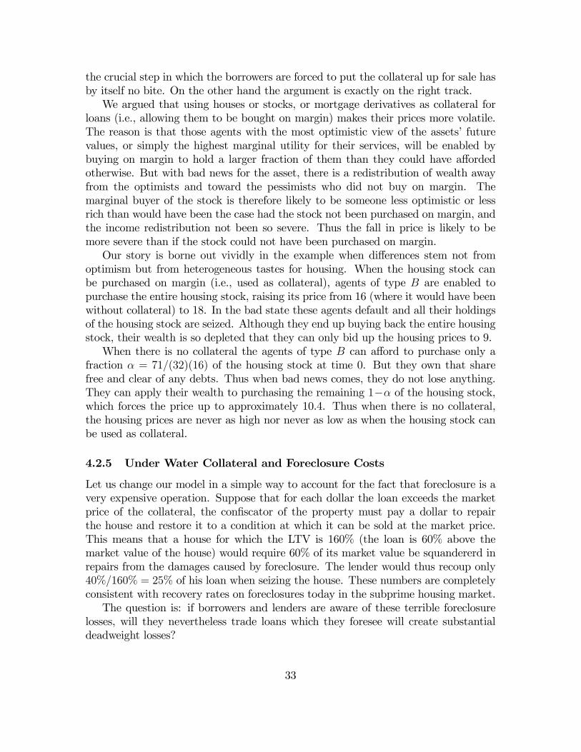
the crucial step in which the borrowers are forced to put the collateral up for sale hasby itself no bite. On the other hand the argument is exactly on the right track.We argued that using houses or stocks, or mortgage derivatives as collateral for

loans (i.e., allowing them to be bought on margin) makes their prices more volatile.The reason is that those agents with the most optimistic view of the assets’ futurevalues, or simply the highest marginal utility for their services, will be enabled bybuying on margin to hold a larger fraction of them than they could have affordedotherwise. But with bad news for the asset, there is a redistribution of wealth awayfrom the optimists and toward the pessimists who did not buy on margin. Themarginal buyer of the stock is therefore likely to be someone less optimistic or lessrich than would have been the case had the stock not been purchased on margin, andthe income redistribution not been so severe. Thus the fall in price is likely to bemore severe than if the stock could not have been purchased on margin.Our story is borne out vividly in the example when differences stem not from

optimism but from heterogeneous tastes for housing. When the housing stock canbe purchased on margin (i.e., used as collateral), agents of type B are enabled topurchase the entire housing stock, raising its price from 16 (where it would have beenwithout collateral) to 18. In the bad state these agents default and all their holdingsof the housing stock are seized. Although they end up buying back the entire housingstock, their wealth is so depleted that they can only bid up the housing prices to 9.When there is no collateral the agents of type B can afford to purchase only a

fraction α = 71/(32)(16) of the housing stock at time 0. But they own that sharefree and clear of any debts. Thus when bad news comes, they do not lose anything.They can apply their wealth to purchasing the remaining 1−α of the housing stock,which forces the price up to approximately 10.4. Thus when there is no collateral,the housing prices are never as high nor never as low as when the housing stock canbe used as collateral.

4.2.5 Under Water Collateral and Foreclosure Costs

Let us change our model in a simple way to account for the fact that foreclosure is avery expensive operation. Suppose that for each dollar the loan exceeds the marketprice of the collateral, the confiscator of the property must pay a dollar to repairthe house and restore it to a condition at which it can be sold at the market price.This means that a house for which the LTV is 160% (the loan is 60% above themarket value of the house) would require 60% of its market value be squandererd inrepairs from the damages caused by foreclosure. The lender would thus recoup only40%/160% = 25% of his loan when seizing the house. These numbers are completelyconsistent with recovery rates on foreclosures today in the subprime housing market.The question is: if borrowers and lenders are aware of these terrible foreclosure

losses, will they nevertheless trade loans which they foresee will create substantialdeadweight losses?

33

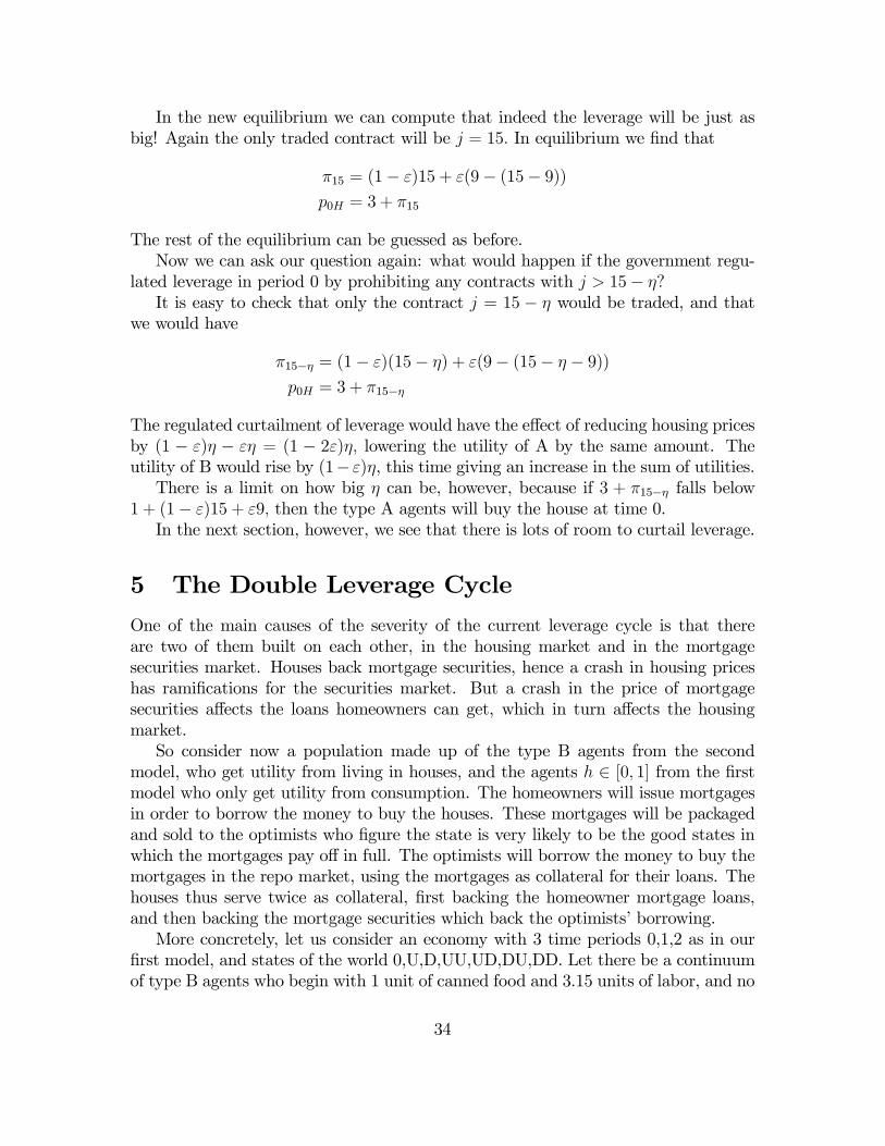
In the new equilibrium we can compute that indeed the leverage will be just asbig! Again the only traded contract will be j = 15. In equilibrium we find that

π15 = (1− ε)15 + ε(9− (15− 9))p0H = 3 + π15

The rest of the equilibrium can be guessed as before.Now we can ask our question again: what would happen if the government regu-

lated leverage in period 0 by prohibiting any contracts with j > 15− η?It is easy to check that only the contract j = 15 − η would be traded, and that

we would have

π15−η = (1− ε)(15− η) + ε(9− (15− η − 9))p0H = 3 + π15−η

The regulated curtailment of leverage would have the effect of reducing housing pricesby (1 − ε)η − εη = (1 − 2ε)η, lowering the utility of A by the same amount. Theutility of B would rise by (1− ε)η, this time giving an increase in the sum of utilities.There is a limit on how big η can be, however, because if 3 + π15−η falls below

1 + (1− ε)15 + ε9, then the type A agents will buy the house at time 0.In the next section, however, we see that there is lots of room to curtail leverage.

5 The Double Leverage Cycle

One of the main causes of the severity of the current leverage cycle is that thereare two of them built on each other, in the housing market and in the mortgagesecurities market. Houses back mortgage securities, hence a crash in housing priceshas ramifications for the securities market. But a crash in the price of mortgagesecurities affects the loans homeowners can get, which in turn affects the housingmarket.So consider now a population made up of the type B agents from the second

model, who get utility from living in houses, and the agents h ∈ [0, 1] from the firstmodel who only get utility from consumption. The homeowners will issue mortgagesin order to borrow the money to buy the houses. These mortgages will be packagedand sold to the optimists who figure the state is very likely to be the good states inwhich the mortgages pay off in full. The optimists will borrow the money to buy themortgages in the repo market, using the mortgages as collateral for their loans. Thehouses thus serve twice as collateral, first backing the homeowner mortgage loans,and then backing the mortgage securities which back the optimists’ borrowing.More concretely, let us consider an economy with 3 time periods 0,1,2 as in our

first model, and states of the world 0,U,D,UU,UD,DU,DD. Let there be a continuumof type B agents who begin with 1 unit of canned food and 3.15 units of labor, and no

34

houses at time 0, and 50 units of canned food in UU,UD,DU, and 9 units of cannedfood in DD, and no other endowments. Suppose that canned food and houses areperfectly durable. Canned food can be eaten at any time, but is durable. We still usethe letter F to describe it. We use the letter L to denote leisure. We shall supposethe marginal utility of leisure (that is, the marginal disutility of labor) is denoted byc.Suppose the type B agents each own a production technology that can take labor

at time 0 and transform 18.15 units into a house a time 0 (that will then be perfectlydurable). Let type B agents assign probability (1−ε) to nature moving up at anystate, and let their utility be

uB(x0F , x0H , x0L, xUUF , xUUH , xUDF , xUDH , xDUF , xDUH , xDDF , xDDH , )

= 9x20F − 2x20F + 15x0H + cx0L + (1− ε)2(xUUF + 15xUUH)+

(1− ε)ε(xUDF + 15xUDH) + ε(1− ε)(xDUF + 15xDUH) + ε2(xDDF + 15xDDH)

((eB0F , eB0H , e

B0L), (e

BUUF , e

BUDF , e

BDUF , e

BDDF ))

= ((1, 0, 3.15), (50, 50, 50, 9))

Note that if the marginal utility of leisure c = 0, then the B agents will always work3.15 hours. But if c is large, then they may choose not to work at all if the wage islow enough.Suppose also there is a continuum of agents h ∈ [0, 1] who are exactly like the

agents in our first model, except that instead of owning one unit of X and Y at time0, they each own 15 units of food and labor at time 0. Agent h ∈ [0, 1] has utilityand endowments

uh(x0F , x0L, x0L, xUF , xDF , xUUF , xUDF , xDUF , xDDF )

= x0F + c̄x0L + hxUF + (1− h)xDF

+ h2xUUF + h(1− h)xUDF + (1− h)hxDUF + (1− h)2xDDF

(eh0F , eh0H , e

h0L) = (15, 0, 15)

The contracts in the economy are of two types, depending on the collateral. Inone kind of contract j, called a mortgage loan of type j, agents can promise the fixedamount j of good F in every one of the last states UU,UD,DU,DD, using one houseas collateral. In the other type of contract k,j called a Repo, agents can promise kunits of good F in every immediate successor state, using contract j as collateral.In our economy, the type B agents will borrow money at time 0 by issuing a

mortgage, using the house they will be constructing at the same time as collateral.The most optimistic agents in [0,1] will buy those mortgages, thereby lending the Bagents the money. Since the mortgages will default in state DD (but not until then),they will be risky. Hence the pessimists will not want to buy those mortgages. But

35

the optmists don’t have enough money to buy them all. So they will borrow moneyfrom the pessimists by selling repo loans against the mortgages they hold. These saferrepo loans will be held by the pessimists. The Repos are one-period loans, unlike themortgage, which is a two-period loan.In a moment we shall define the equilibrium formally, but in view of our earlier

analysis, it is easy to describe now. We normalize by taking the price of canned foodto be 1 in every state. In equilibrium the price of labor in period 0 will be .95. Theincome of the B agents at time 0 is then 1 + (3.15)(.95) = 4. By constant returns toscale, the price of the house will then be (18.15)(.95) = (3.15+15)(.95) = 3+14.25 =17.25. The B agents will each buy a house by putting 3 dollars down and borrowingthe remaining 14.25 by issuing a mortgage j=15 promising 15 in every state in thelast period.Let us make the hypothesis that if the house is underwater by y dollars when the

loan comes due, then y dollars must be wasted in order to restore the house to mintcondition to sell on a par with the other houses on the market. In all the terminalstates except DD, the prices will not be underwater, and the house will sell for 15.But in DD the house will only sell for 9, which means it will be underwater, and themortgage will only deliver 9-(15-9)=3 to the mortgage holder after he confiscates thehouse and sells it, net of the restoration costs.We see that the terminal payoffs of the mortgage security is thus (15,15,15,3),

which is 15 times the terminal price of the security in our first example. The agentsof type h each own 15 units of the canned food, exactly 15 times what they ownedof the durable consumption good before, and their labor income is exactly enoughto buy one mortgage security, again 15 times as valuable as the security in our firstexample. Hence this equilibrium we are computing is just the one in our first examplescaled up by a factor of 15.In state D the mortgage will be worth 15(.69) dollars. In state 0, the top 13%

of agents h will buy the mortgages by issuing repos promising k=15(.69). In stateD these optimists will be wiped out, and the mortgages will fall into the hands ofmore pessimistic investors. Agents h ∈ [.61, .87) will buy the mortgage securities atD, issuing contract (j,k)=(15,3) in the repo market to obtained borrowed money tohelp them buy it. Part of the reason the price of mortgages is so low at D is that thepayoffs are so bad at DD, which limits not just the value but the amount of leveragethat can be obtained at D.We see that there is a double leverage cycle. At 0 homeowners leveraged too much

in the mortgage market, and investors leveraged their mortgage purchases too muchin the repo markets. At D there is massive deleveraging in the securities market,and no opportunity for leverage in the housing market, since the homeowners are allunder water and cannot sell their houses.

36

5.1 What’s so bad about the leverage cycle?

In the leverage cycle asset prices shoot up and shoot down as leverage changes. Thisdrastic change is unsettling in any real economy, and I would argue is a danger in andof itself. But why is this so bad in welfare terms? In our first example, the same kindof asset gyrations would occur with complete markets, though on a different scale. Inthe second example, however, asset prices would have remained stable between U andD with complete markets, while with collateral and incomplete markets they drop by50% between U and D. If complete markets is our benchmark, then we see evidenceof a problem already.But the real danger I believe is that when asset prices collapse, new activity

plunges as well. Why would anyone want to buy a new mortgage, to enable a newbuilder, when the old mortgages are so cheap? Let us re-examine our double leveragecycle.Imagine now that in addition to the agents already described, there is a new

generation of B’ agents born at U and at D, with the same utilities over youthfulconsumption and over terminal consumption as before. Imagine also that we give theh agents 15 more units of labor endowment at U and at D, but no more income offood. Let us allow the new generation to write mortgages just like the old ones did,payable in the terminal states. Will the new generation be able to build houses likethe old?The answer at U is yes, but at D is emphatically no. The most optimistic agents

will have already gone broke by D, and the leverage on mortgages is very low, so theprice of mortgages will be much lower at D than at 0. Thus the B’ agents will notbe able to borrow nearly as much to buy the house, and thus will not be able to hirethe labor necessary to build it.Homeowners do recognize that by leveraging so much, they are tumbling further

under water at DD, reducing the payoffs to the lender there and thereby reducing theincrease in the amount they can borrow by promising more. A key externality theydo not recognize, however, is that by doing so they limit how much the optimists canleverage at D, and therefore also at 0, and therefore they fail to recognize that theyare reducing the value of the mortgages they want to sell. Similarly, the optimistswho leverage so much at 0 overlook the fact that if they had tempered their leverage,they would be ina better position to buy mortgages at D, which would have raisedthe price of houses at D, which might have led to their further employment at D.Need to finish calculating this.

6 References

The presentation is based on the following:Geanakoplos, John. 1997. “Promises, Promises.” In The Economy as an Evolving

Complex System II, ed. W. Brian Arthur, Steven Durlauf, and David Lane, 285—320.

37

Reading, MA: Addison-Wesley.Geanakoplos, John. 2003. “Liquidity, Default, and Crashes: Endogenous Con-

tracts in General Equilibrium.” In Advances in Economics and Econometrics: Theoryand Applications, Eighth World Conference,Vol. 2, 170—205. Econometric SocietyMonographs.Fostel A., Geanakoplos J. 2008. “Leverage Cycles and the Anxious Economy”

Lead article American Economic Review 2008, 98:4, 1211-1244.

Some Relevant References are:

Bernanke, Ben, Mark Gertler and Simon Gilchrist. 1996. “The Financial Accela-tor and the Flight to Quality.” Review of Economics and Statistics, 78(1): 1—15.Brunnermeier, Markus, and Llasse Pedersen. “Market Liquidity and Funding

Liquidity.”Review of Financial Studies.Caballero, Richardo J., and Arvind Krishnamurthy. 2001. “International and

Domestic Collateral Constraints in a Model of Emerging Market Crises.” Journal ofMonetary Economics, 48(3): 513—48.Fostel, Ana, and John Geanakoplos. 2008. “Collateral Restrictions and Liquidity

under-Supply: A Simple Model.” Economic Theory, 35(3): 441—67.Kiyotaki, Nobuhiro, and John Moore. 1997. “Credit Cycles.” Journal of Political

Economy, 105(2): 211—48.Morris, S., Shin, H. 2004. Liquidity black holes. Review of Finance, 8, 1-18Tobias A, Shin H. “Liquidity and Leverage”. Forthcoming in the Journal of

Financial IntermediationVayanos, Dimitri. 2004. “Flight to Quality, Flight to Liquidity, and the Pricing

of Risk.” Unpublished.

38