Leverage and Deepening

Business Cycle Skewness∗

Henrik Jensen† Ivan Petrella‡

Søren Hove Ravn§ Emiliano Santoro¶

August 2017

Abstract

We document that the U.S. economy has been characterized by an increasingly negativebusiness cycle asymmetry over the last three decades. This finding can be explained bythe concurrent increase in the financial leverage of households and firms. To supportthis view, we devise and estimate a dynamic general equilibrium model with collateral-ized borrowing and occasionally binding credit constraints. Higher leverage increases thelikelihood that constraints become slack in the face of expansionary shocks, while con-tractionary shocks are further amplified due to binding constraints. As a result, boomsbecome progressively smoother and more prolonged than busts. We are therefore able toreconcile a more negatively skewed business cycle with the Great Moderation in cyclicalvolatility. Finally, in line with recent empirical evidence, financially-driven expansionslead to deeper contractions, as compared with equally-sized non-financial expansions.

Keywords: Credit constraints, business cycles, skewness, deleveraging.JEL: E32, E44.

∗We thank– without implicating– Juan Antolín-Diaz, Henrique Basso, Thomas Drechsel, Alessandro Galesi,Tom Holden, Kieran Larkin, Alisdair McKay, Gabriel Perez-Quiros, Omar Rachedi, Federico Ravenna, LucaSala, Yad Selvakumar, Marija Vukotic, and seminar participants at Banco de España, Goethe University Frank-furt, Danmarks Nationalbank, Catholic University of Milan, the “Workshop on Macroeconomic and FinancialTime Series Analysis”at Lancaster University, the “4th Workshop in Macro, Banking and Finance”at SapienzaUniversity of Rome, the “7th IIBEO Alghero Workshop”at the University of Sassari, the “12th Dynare Confer-ence”at the Banca d’Italia, the “8th Nordic Macroeconomic Summer Symposium”in Ebeltoft, the “3rd BCAMAnnual Workshop”at Birkbeck, University of London, and the “2017 Computation in Economics and FinanceConference”at Fordham University in New York for helpful comments and suggestions. Part of this work hasbeen conducted while Santoro was visiting Banco de España, whose hospitality is gratefully acknowledged. Thispaper was previously circulated under the title “Deepening Contractions and Collateral Constraints”.†University of Copenhagen and CEPR. Department of Economics, University of Copenhagen, Øster

Farimagsgade 5, Bld. 26, 1353 Copenhagen, Denmark. E-mail : Henrik.Jensen@econ.ku.dk.‡University of Warwick and CEPR. Warwick Business School, University of Warwick, Scarman Rd, CV4

7AL Coventry, United Kingdom. E-mail : Ivan.Petrella@wbs.ac.uk.§University of Copenhagen. Department of Economics, University of Copenhagen, Øster Farimagsgade 5,

Bld. 26, 1353 Copenhagen, Denmark. E-mail : Soren.Hove.Ravn@econ.ku.dk.¶University of Copenhagen. Department of Economics, University of Copenhagen, Øster Farimagsgade 5,

Bld. 26, 1353 Copenhagen, Denmark. E-mail : Emiliano.Santoro@econ.ku.dk.

1 Introduction

Economic fluctuations across the industrialized world are typically characterized by asymme-

tries in the shape of expansions and contractions in aggregate activity. A prolific literature

has extensively studied the statistical properties of this empirical regularity, reporting that

the magnitude of contractions tends to be larger than that of expansions; see, among others,

Neftci (1984), Hamilton (1989), Sichel (1993) and, more recently, Morley and Piger (2012).

While these studies have generally indicated that business fluctuations are negatively skewed,

the possibility that business cycle asymmetry has changed over time has been overlooked. Yet,

the shape of the business cycle has evolved over the last three decades: For instance, since

the mid-1980s the U.S. economy has displayed a marked decline in macroeconomic volatility,

a phenomenon known as the Great Moderation (Kim and Nelson, 1999; McConnell and Perez-

Quiros, 2000). This paper documents that, over the same period, the skewness of the U.S.

business cycle has become increasingly negative. Our key contribution is to show that occa-

sionally binding financial constraints, combined with a sustained increase in financial leverage,

allow us to account for several facts associated with the evolution of business cycle asymmetry.

Figure 1 reports the post-WWII rate of growth of U.S. real GDP, together with the 68%

and 90% confidence intervals from a Gaussian density fitted on pre- and post-1984 data. Three

facts stand out: First, as discussed above, the U.S. business cycle has become less volatile in

the second part of the sample, even if we take into account the major turmoil induced by the

Great Recession. Second, real GDP growth displays large swings in both directions during the

first part of the sample, while in the post-1984 period the large downswings associated with the

three recessionary episodes are not matched by similar-sized upswings. In fact, if we examine

the size of economic contractions in conjunction with the drop in volatility occurring since the

mid-1980s, it appears that recessions have become relatively more ‘violent’, whereas the ensuing

recoveries have become smoother, as recently pointed out by Fatás and Mihov (2013). Finally,

recessionary episodes have become less frequent, thus implying more prolonged expansions.

[Insert Figure 1]

These properties translate into the U.S. business cycle becoming more negatively skewed

over the last three decades. Explaining this pattern represents a challenge for existing business

cycle models. To meet this, a theory is needed that involves both non-linearities and a secular

development of the underlying mechanism, so as to shape the evolution in the skewness of

the business cycle. As for the first prerequisite, the importance of borrowing constraints as

1

a source of business cycle asymmetries has long been recognized in the literature; see, e.g.,

the survey by Brunnermeier et al. (2013). In expansions, households and firms may find it

optimal to borrow less than their available credit limit. Instead, financial constraints tend to

be binding during recessions, so that borrowing is tied to the value of collateral assets. The

resulting non-linearity translates into a negatively skewed business cycle. As for the second

prerequisite, the past decades have witnessed a major deregulation of financial markets, with

one result being a substantial increase in the degree of leverage of advanced economies. To see

this, Figure 2 reports the credit-to-GDP and the loan-to-asset (LTA) ratios of both households

and the corporate sector in the US.1 This leveraging process is also confirmed, e.g., by Jordà

et al. (2017) in a large cross-section of countries.

[Insert Figure 2]

Based on these insights, the objective of this paper is to propose a structural explanation of

deepening business cycle skewness. To this end, we devise and estimate a dynamic stochastic

general equilibrium (DSGE) model that allows for the collateral constraints faced by the firms

and a fraction of the households not to bind at all points in time. We show that an increase

in leverage raises the likelihood of financial constraints becoming slack in the face of expan-

sionary shocks, dampening the magnitude of the resulting boom. By contrast, in the face of

contractionary shocks borrowers tend to remain financially constrained, with debt reduction

becoming more burdensome as leverage increases. In light of this mechanism, the skewness of

the business cycle becomes increasingly negative. As in the data, the model also predicts that

the duration of business cycle contractions does not change much as leverage increases, while

the duration of expansions almost doubles.

We then juxtapose the drop in the skewness of the business cycle with the Great Moderation

in macroeconomic volatility. While increasing LTV ratios cannot fully account for the Great

Moderation, our analysis shows that the increase in the asymmetry of the business cycle is

compatible with a drop in its volatility. Additionally, the decline in macroeconomic volatility

mostly rests on the characteristics of the expansions, whose magnitude declines as an effect

of collateral constraints becoming increasingly non-binding in the face of higher credit limits.

This is in line with the recent empirical findings of Gadea-Rivas et al. (2014, 2015), who show

that neither changes to the depth nor to the frequency of recessionary episodes account for the

1As we discuss in Appendix A, the aggregate loan-to-asset ratios reported in Figure 2 are likely to understatethe actual LTV ratios requirements faced by the marginal borrower. While alternative measures may yieldhigher LTV ratios, they point to the same behavior of leverage over time (see also Graham et al., 2014, andJordà et al., 2017).

2

stabilization of macroeconomic activity in the US.2

Recently, increasing attention has been devoted to the connection between the driving fac-

tors behind business cycle expansions and the extent of the subsequent contractions. Jordà et al.

(2013) report that more credit-intensive expansions tend to be followed by deeper recessions–

irrespective of whether the latter are accompanied by a financial crisis. Our model accounts

for this feature along two dimensions. First, we show that contractions become increasingly

deeper as the average LTV ratio increases, even though the boom-bust cycle is generated by

the same combination of expansionary and contractionary shocks. Second, financially-driven

expansions lead to deeper contractions, when compared to similar-sized expansions generated

by non-financial shocks. Both exercises emphasize that, following a contractionary shock,

the aggregate repercussions of constrained agents’deleveraging increases in the size of their

debt. As a result, increasing leverage makes it harder for savers to compensate for the drop

in consumption and investment of constrained agents. This narrative of the boom-bust cycle

characterized by a debt overhang is consistent with the results of Mian and Sufi (2010), who

identify a close connection at the county level in the US between pre-crisis household leverage

and the severity of the Great Recession. Likewise, Giroud and Mueller (2017) document that,

over the same period, counties with more highly leveraged firms suffered larger employment

losses.

A key prediction of our model is that financial constraints on both households and firms

have become less binding during the last three decades. This claim is consistent with existing

accounts of the widespread financial liberalization that started in the US during the 1980s,

which provide evidence of a relaxation of financial constraints over time (see, e.g., Justiniano

and Primiceri, 2008). For households, Dynan et al. (2006) and Campbell and Hercowitz (2009)

have discussed how the wave of financial deregulation taking place in the early 1980s paved

the way for a substantial reduction in downpayment requirements and the rise of the subprime

mortgage market. Combined with the boom in securitization some years later, this profoundly

transformed household credit markets and gave rise to the leveraging process observed in Fig-

ure 2. Indeed, Guerrieri and Iacoviello (2017) report that non-binding credit constraints were

prevalent among U.S. households from the late 1990s until the onset of the Great Recession.

2In this respect, downward wage rigidity has recently been pointed to as an alternative source of macroeco-nomic asymmetry (see Abbritti and Fahr, 2013). However, for this to act as a driver of deepening businesscycle asymmetry, one would need to observe stronger rigidity over time, which does not seem to be the case.Most importantly, even if such a mechanism was at work, the resulting change in the skewness of the businesscycle would primarily rest on the emergence of more dramatic recessionary episodes, without any major changein the key characteristics of expansions. However, this implication would stand in contrast with the evidenceof Gadea-Rivas et al. (2014, 2015).

3

For businesses, the period since around 1980 has witnessed the emergence of a market for high-

risk, high-yield bonds (Gertler and Lown, 1999) along with enhanced access to both equity

markets and bank credit for especially small- and medium-sized firms (Jermann and Quadrini,

2009). Over the same period the investment-cash flow sensitivity in the US has declined sub-

stantially, a fact interpreted by several authors as an alleviation of firms’financial frictions (see,

e.g., Agca and Mozumdar, 2008, and Brown and Petersen, 2009). Our findings point to these

developments as an impetus of the deepening skewness of the U.S. business cycle observed

during the same period.

The observation that occasionally binding credit constraints may give rise to macroeconomic

asymmetries is not new. Mendoza (2010) explores this idea in the context of a small open

economy facing a constraint on its access to foreign credit. As this constraint becomes binding,

the economy enters a ‘sudden stop’episode characterized by a sharp decline in consumption. In

related work, Maffezzoli and Monacelli (2015) show that the aggregate implications of financial

shocks are state-dependent, with the economy’s response being greatly amplified in situations

where agents switch from being financially unconstrained to being constrained. In a similar

spirit, Guerrieri and Iacoviello (2017) report that house prices exerted a much larger effect on

private consumption during the Great Recession– when credit constraints became binding–

than in the preceding expansion. While all these studies focus on specific economic disturbances

and/or historical episodes, a key insight of this paper is to show how different evolving traits of

business cycle asymmetry may be accounted for by a secular process of financial liberalization,

conditional on both financial and non-financial disturbances.

Our paper lends support to a recent empirical literature that focuses on the connection

between leverage and business cycle asymmetry. Among various other business cycle facts,

Jordà et al. (2017) report a positive correlation between the skewness of real GDP growth and

the credit-to-GDP ratio for a large cross-section of countries observed over a long time-span.

Popov (2014) exclusively focuses on business cycle asymmetry in a large panel of developed

and developing countries, documenting two main results. First, the average business cycle

skewness across all countries became markedly negative after 1991, consistent with our findings

for the US. Second, this pattern is particularly distinct in countries that liberalized their

financial markets. Also Bekaert and Popov (2015) examine a large cross-section of countries,

reporting that more financially developed economies have more negatively skewed business

cycles. Finally, Rancière et al. (2008) establish a negative cross-country relationship between

real GDP growth and the skewness of credit growth in financially liberalized countries. While

4

we focus on the asymmetry of output, we observe a similar pattern for credit, making our

results comparable with their findings. On a more general note, all of these studies focus

on the connection between business cycle skewness and financial factors in the cross-country

dimension, whereas we examine how financial leverage may have shaped various dimensions of

business cycle asymmetry over time.

The rest of the paper is organized as follows. In Section 2 we report evidence on the

connection between leverage and changes in the shape of the business cycle in the US. Section

3 inspects the key mechanisms at play in our narrative within a simple two-period model.

Section 4 presents our DSGE model, and Section 5 discusses the solution and estimation.

Section 6 reports the main results. Section 7 shows that the model is capable of producing the

type of debt overhang recession emphasized in recent empirical studies. Section 8 concludes.

The Appendices contain supplementary material concerning the model solution and various

empirical and computational details.

2 Empirical evidence

We first examine various aspects of business cycle asymmetry and how they changed over the

last three decades. We then take advantage of cross-sectional variation across the U.S. States to

document an empirical relationship between household leverage and the deepness of state-level

contractions during the Great Recession.

2.1 Changing business cycle asymmetry

A number of empirical studies have documented a major reduction in the volatility of the U.S.

business cycle since the mid-1980s. In this section we document changes in the asymmetry of

the cycle that have occurred over the same timespan. Table 1 reports the skewness of the rate

of growth of different macroeconomic aggregates in the pre- and post-1984 period.

[Insert Table 1]

The skewness is typically negative and not too distant from zero in the first part of the

sample, but becomes more negative thereafter.3 ,4 To supplement these findings, Figure 3 reports

3Appendix B1 reports measures of time-varying volatility and skewness of real GDP growth, based on anon-parametric estimator. The downward pattern in business cycle asymmetry emerges as a robust feature ofthe data, along with the widely documented decline in macroeconomic volatility.

4A drop in the skewness of GDP growth has also been pointed out in recent work by Garín et al. (2017). Thepresent section expands on their finding in a number of directions, primarily by showing that the drop in the

5

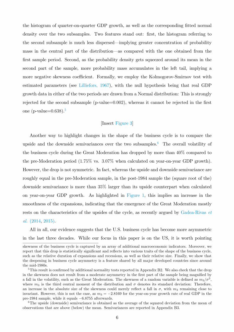
the histogram of quarter-on-quarter GDP growth, as well as the corresponding fitted normal

density over the two subsamples. Two features stand out: first, the histogram referring to

the second subsample is much less dispersed– implying greater concentration of probability

mass in the central part of the distribution– as compared with the one obtained from the

first sample period. Second, as the probability density gets squeezed around its mean in the

second part of the sample, more probability mass accumulates in the left tail, implying a

more negative skewness coeffi cient. Formally, we employ the Kolmogorov-Smirnov test with

estimated parameters (see Lilliefors, 1967), with the null hypothesis being that real GDP

growth data in either of the two periods are drawn from a Normal distribution: This is strongly

rejected for the second subsample (p-value=0.002), whereas it cannot be rejected in the first

one (p-value=0.638).5

[Insert Figure 3]

Another way to highlight changes in the shape of the business cycle is to compare the

upside and the downside semivariances over the two subsamples.6 The overall volatility of

the business cycle during the Great Moderation has dropped by more than 40% compared to

the pre-Moderation period (1.75% vs. 3.07% when calculated on year-on-year GDP growth).

However, the drop is not symmetric. In fact, whereas the upside and downside semivariance are

roughly equal in the pre-Moderation sample, in the post-1984 sample the (square root of the)

downside semivariance is more than 35% larger than its upside counterpart when calculated

on year-on-year GDP growth. As highlighted in Figure 1, this implies an increase in the

smoothness of the expansions, indicating that the emergence of the Great Moderation mostly

rests on the characteristics of the upsides of the cycle, as recently argued by Gadea-Rivas et

al. (2014, 2015).

All in all, our evidence suggests that the U.S. business cycle has become more asymmetric

in the last three decades. While our focus in this paper is on the US, it is worth pointing

skewness of the business cycle is captured by an array of additional macroeconomic indicators. Moreover, wereport that this drop is statistically significant and reflects into various traits of the shape of the business cycle,such as the relative duration of expansions and recessions, as well as their relative size. Finally, we show thatthe deepening in business cycle asymmetry is a feature shared by all major developed countries since aroundthe mid-1980s.

5This result is confirmed by additional normality tests reported in Appendix B2. We also check that the dropin the skewness does not result from a moderate asymmetry in the first part of the sample being magnified bya fall in the volatility, such as the Great Moderation. The skewness of a random variable is defined as m3/σ3,where m3 is the third central moment of the distribution and σ denotes its standard deviation: Therefore,an increase in the absolute size of the skewness could merely reflect a fall in σ, with m3 remaining close toinvariant. However, this is not the case, as m3 = −2.8169 for the year-on-year growth rate of real GDP in thepre-1984 sample, while it equals −6.8755 afterwards.

6The upside (downside) semivariance is obtained as the average of the squared deviation from the mean ofobservations that are above (below) the mean. Semivariances are reported in Appendix B3.

6

out that a similar pattern emerges across the G7 economies, as we show in Appendix B4.

Combined with the finding of Jordà et al. (2017) that secular increases in financial leverage

are widespread across advanced economies, this suggests that our narrative may have wider

relevance.

The next step in the analysis consists of translating changes in the business cycle asymmetry

into some explicit measure of the deepness of economic contractions, while accounting for time-

variation in the dispersion of the growth rate process. In line with Jordà et al. (2017), the

first column of Table 2 reports the fall of real GDP during a given recession, divided by the

duration of the recession itself: this measure is labelled as ‘violence’.7

[Insert Table 2]

Comparing the violence of the contractionary episodes before and after 1984, we notice that

the 1991 and 2001 recessions have not been very different from earlier contractions. However, to

compare the relative magnitude of different recessions over a period that displays major changes

in the volatility of the business cycle, it is appropriate to control for the average variability of

the cycle around a given recessionary episode. To this end, the second column of Table 2 reports

standardized violence, which is obtained by normalizing violence by a measure of the variability

of real GDP growth.8 Using this metric we get a rather different picture. The three recessionary

episodes occurred during the Great Moderation are substantially deeper than the pre-1984 ones:

averaging out the first seven recessionary episodes returns a standardized violence of 1.22%,

against an average of 2.90% for the post-1984 period. Moreover, as highlighted in the last two

columns of Table 2, the duration of business cycle contractions does not change much between

the two samples, while the duration of the expansions doubles. This contributes to picturing

the business cycle in the post-1984 sample as consisting of more smoothed and prolonged

expansions, interrupted by shorter– yet, more dramatic– contractionary episodes.

2.2 Leverage and business cycle asymmetry: cross-state evidence

So far we have established that the post-1984 period is characterized by a smoother path of

the expansionary periods and a stronger standardized violence of the recessionary episodes, as

7For earlier analyses on the violence and brevity of economic contractions see Mitchell (1927) and, morerecently, McKay and Reis (2008).

8The volatility is calculated as the standard deviation of the year-on-year growth rate of real GDP over a5-year window. We exclude the period running up to the recession by calculating the standard deviation up toa year before the recession begins. Weighting violence by various alternative mesures of business cycle volatilityreturns a qualitatively similar picture: Appendix B5 reports additional robustness evidence on the standardizedviolence of the recessions in the US.

7

compared with the pre-1984 period. In addition, over the same time window the process of

financial deregulation has been associated with a sizeable increase in leverage of both households

and firms. Relying on county-level US data, Mian and Sufi(2010) have identified a strong causal

link between pre-crisis household leverage and the severity of the Great Recession. We now

produce related evidence based on state-level data. Specifically, we take data on quarterly real

Gross State Product (GSP) from the BEA Regional Economic Accounts and compute both the

skewness of GSP growth and the violence of the Great Recession in the U.S. States.9 Figure

4 correlates the resulting statistics to the average debt-to-income ratio prior to the recession.

Notably, states where households were more leveraged not only have witnessed more severe

GSP contractions during the last recession, but have also displayed a more negatively skewed

GSP growth over the 2005-2016 time window. These findings echo those of Mian and Sufi

(2010).

[Insert Figure 4]

To gain further insights into the cross-sectional connection between the magnitude of the

Great Recession and business cycle dynamics, we order the U.S. states according to households’

average pre-crisis debt-to-income ratio. We then construct two synthetic series, computed as the

growth rates of the median real GSP of the top and the bottom ten states in terms of leverage,

respectively. According to Figure 5, there are no noticeable differences in the performance of

the two groups before and after the Great Recession, with both of them growing at a roughly

similar pace. However, the drop in real activity has been much deeper for relatively more

leveraged states. Altogether, this evidence points to a close link between leverage and business

cycle asymmetries.

[Insert Figure 5]

3 A simple two-period model

Some preliminary insights into our main analysis can be offered through a simple two-period

model of collateralized debt. The model shares many of the central aspects of our DSGE

model, most notably an asset-based credit constraint. A representative household has utility

9To account for the possibility that the recession does not begin/end in the same period across the US, wedefine the start of the recession in a given state as the period with the highest level of real GSP in the windowthat goes from five quarters before the NBER peak date to one quarter after that. Similarly, the end of therecession is calculated as the period with the lowest real GSP in the window from one quarter before to fivequarters after the NBER trough date.

8

U = E0∑2

t=1 βt−1[a logCt + (1− a) logHt]

, a ∈ (0, 1), β ∈ (0, 1), where Ct and Ht denote

the consumption of a nondurable good and (non-depreciating) land, respectively. In period

1, households’budget constraint is C1 + Q1 (H1 −H0) − B1 = Y1 − RB0, where B0 is initial

debt, R > 1 is a constant gross real rate of interest, and Y1 is a stochastic endowment, with F

indicating its cumulative distribution function. We denote by Q1 the price of land relative to

that of nondurables. As in Kiyotaki and Moore (1997), the stock of debt in period 1 cannot

exceed a fraction of the present value of land:

B1 ≤ sE1 Q2H1

R, s ∈ [0, 1] , (1)

with s representing the loan-to-value ratio. In period 2, households are assumed to pay back,

with interest, any acquired debt– irrespective of whether (1) was binding or not. Assuming

a deterministic endowment Y in period 2, households therefore face the budget constraint

C2 +Q2 (H2 −H1) = Y −RB1. We assume that land is inelastically supplied in both periods.

Appendix C shows in detail the derivation of the model’s competitive equilibrium, but here

it suffi ces to consider the resulting nondurable consumption in period 1. When the constraint

(1) is binding, we obtain

C1 = Y1 −RB0 +s (1− a)

a+ s (1− a)

Y

R. (2)

If (1) does not bind, instead, we retrieve the following solution:

C1 =1

1 + β(Y1 −RB0) +

1

R (1 + β)Y. (3)

Several insights emerge from this simple set-up. A comparison of (2) and (3) reveals how

negative skewness arises in connection with the tightness of the credit constraint. Variations in

Y1 affect consumption much stronger when the credit constraint binds, as compared to when

it is slack. Not surprisingly, in financially-constrained states households behave according to a

hand-to-mouth protocol, with a marginal propensity to consume out of current income equal

to one. In financially-unconstrained states, on the other hand, households are able to smooth

their lifetime resources across periods, implying a marginal propensity to consume of 1/ (1 + β).

Now assume to start out at Y1 = Y 1, where Y 1 is the income that equalizes C1 given by (2) and

(3), respectively. This ‘trigger value’of income is the minimum value of income securing that

(1) becomes slack; see Appendix C for further details. If a ‘good’shock hits (i.e., Y1 = Y 1+ ∆,

∆ > 0), consumption increases by ∆/ (1 + β), as (1) becomes non-binding. If a similar-sized

‘bad’shock hits (i.e., Y1 = Y 1 −∆), consumption drops by ∆ > ∆/ (1 + β) since (1) becomes

9

binding. Hence, consumption downturns are deeper than upturns.

From (2) we can see how the credit limit s, and thus financial leverage, plays a central role.

Higher s means that more debt can be acquired in the constrained regime. Ceteris paribus,

this implies that the household is less likely to become credit constrained. We formalize this

argument by deriving Y 1:

Y 1 = RB0 +a− βs (1− a)

a+ s (1− a)

Y

βR. (4)

Since Y1 ≤ Y 1 results in a binding constraint, the probability that the credit constraint binds

is F(Y 1

). From (4), it follows that higher s, and thus higher leverage, decreases Y 1 and the

probability of the constraint being binding, as F ′ > 0.

The next section introduces an estimated DSGE model where the mechanisms we have

just described produce increasingly negative asymmetry, due to the financial constraints faced

by different types of borrowers becoming more often slack in connection with a process of

financial leveraging. Essentially, in such a model aggregate dynamics emerges as a mixture of

the behavioral rules governing consumption and investment decisions under different regimes.

A higher probability of non-binding financial constraints will be associated with more marked

asymmetries, as those documented in Section 2.

4 A DSGE model

We adopt a standard real business cycle model augmented with collateral constraints, along

the lines of Kiyotaki and Moore (1997), Iacoviello (2005), Liu et al. (2013), and Justiniano

et al. (2015); inter alia. The economy is populated by three types of agents, each of mass

one. These agents differ by their discount factors, with the so-called patient households dis-

playing the highest degree of time preference, while impatient households and entrepreneurs

have relatively lower discount factors. Moreover, patient and impatient households supply la-

bor, consume nondurable goods and land services. Entrepreneurs only consume nondurable

goods, and accumulate both land and physical capital, which they rent to firms. The latter are

of unit mass and operate under perfect competition, taking labor inputs from both types of

households, along with capital and land from the entrepreneurs. The resulting gross product

may be used for investment and nondurable consumption.

10

4.1 Patient households

The utility function of patient households is given by:

E0

∞∑t=0

(βP)t [

log(CPt − θPCP

t−1)

+ εt log(HPt

)+

νP

1− ϕP(1−NP

t

)1−ϕP ], (5)

0 < βP < 1, ϕP ≥ 0, ϕP 6= 1, νP > 0, 0 ≤ θP < 1

where CPt denotes their nondurable consumption, H

Pt denotes land holdings, and N

Pt denotes

the fraction of time devoted to labor. Moreover, βP is the discount factor, θP measures the

degree of habit formation in nondurable consumption and ϕP is the coeffi cient of relative risk

aversion pertaining to leisure. Finally, εt is a land-preference shock satisfying

log εt = log ε+ ρε (log εt−1 − log ε) + ut, 0 < ρε < 1, (6)

where ε > 0 denotes the steady-state value and where ut ∼ N (0, σ2ε). Utility maximization is

subject to the budget constraint

CPt +Qt

(HPt −HP

t−1)

+Rt−1BPt−1 = BP

t +W Pt N

Pt , (7)

where BPt denotes the stock of one-period debt held at the end of period t, Rt is the associated

gross real interest rate, Qt is the price of land in units of consumption goods, and W Pt is the

real wage.

4.2 Impatient households

The utility of impatient households takes the same form as that of patient households:

E0

∞∑t=0

(βI)t [

log(CIt − θICI

t

)+ εt log

(HIt

)+

νI

1− ϕI(1−N I

t

)1−ϕI], (8)

0 < βI < βP , ϕI > 0, ϕI 6= 1, νI > 0, 0 ≤ θI < 1

where, as for the patient households, CIt denotes nondurable consumption, H

It denotes land

holdings, and N It denotes the fraction of time devoted to labor. Households’difference in the

degree of time preference is captured by imposing βP > βI . This ensures that, in the steady

state, patient and impatient households act as lenders and borrowers, respectively. Impatient

11

households are subject to the following budget constraint

CIt +Qt

(HIt −HI

t−1)

+Rt−1BIt−1 = BI

t +W It N

It . (9)

Moreover, impatient households are subject to a collateral constraint, according to which

their borrowing BIt is bounded above by a fraction s

It of the expected present value of land

holdings at the beginning of period t+ 1:

BIt ≤ sIt

Et Qt+1HIt

Rt

, (10)

This constraint can be rationalized in terms of limited enforcement, as in Kiyotaki and Moore

(1997). The loan-to-value (LTV) ratio (or credit limit), sIt , is stochastic and aims at capturing

financial shocks (as in, e.g., Jermann and Quadrini, 2012 and Liu et al., 2013):

log sIt = log sI + log st (11)

log st = ρs log st−1 + vt, 0 < ρs < 1, (12)

where vt ∼ N (0, σ2s) and sI , the steady-state LTV ratio, is a proxy for the average stance of

credit availability to the impatient households.

4.3 Entrepreneurs

Entrepreneurs have preferences over nondurables only (see Iacoviello, 2005; Liu et al., 2013),

and maximize

E0

∞∑t=0

(βE)t

log(CEt − θECE

t−1)

, 0 < βE < βP , 0 ≤ θE < 1, (13)

where CEt denotes entrepreneurial nondurable consumption. Utility maximization is subject

to the following budget constraint

CEt + It +Qt

(HEt −HE

t−1)

+Rt−1BEt−1 = BE

t + rKt−1Kt−1 + rHt−1HEt−1, (14)

where It denotes investment in physical capital, Kt−1 is the physical capital stock rented to

firms at the end of period t − 1, and HEt−1 is the stock of land rented to firms. Finally, r

Kt−1

and rHt−1 are the rental rates on capital and land, respectively. Capital depreciates at the rate

δ, and its accumulation is subject to investment adjustment costs determined by Ω, so that its

12

law of motion reads as

Kt = (1− δ)Kt−1 +

[1− Ω

2

(ItIt−1− 1

)2]It, 1 > δ > 0, Ω > 0. (15)

Like impatient households, entrepreneurs are credit constrained, but they are able to use both

capital and their holdings of land as collateral:10

BEt ≤ sEt Et

QKt+1Kt +Qt+1H

Et

Rt

, (16)

where QKt denotes the price of installed capital in consumption units and s

Et behaves in accor-

dance with

log sEt = log sE + log st, (17)

where sE denotes entrepreneurs’steady-state LTV ratio.11 Together with households’average

LTV ratio, this parameter will assume a key role in the analysis of the evolving connection

between macroeconomic asymmetries and financial leverage.

4.4 Firms

Firms operate under perfect competition, employing a constant-returns-to-scale technology.

They rent capital and land from the entrepreneurs and hire labor from both types of households

in order to maximize their profits. The production technology for output, Yt, is given by:

Yt = At

[(NPt

)α (N It

)1−α]γ [(HEt−1)φK1−φt−1

]1−γ, 0 < α, φ, γ < 1, (18)

with total factor productivity At evolving according to

logAt = logA+ ρA (logAt−1 − logA) + zt, 0 < ρA < 1, (19)

where A > 0 is the steady-state value of At, and zt ∼ N (0, σ2A).

10The importance of real estate as collateral for business loans has recently been emphasized by Chaney etal. (2012) and Liu et al. (2013).11As we will discuss in Section 5.1.2, the LTA series are cointegrated and their deviations from the common

trend are highly correlated, so we opt for a single financial shock.

13

4.5 Market clearing

Aggregate supply of land is fixed at H, implying that land-market clearing is given by

H = HPt +HI

t +HEt . (20)

The economy-wide net financial position is zero, such that

BPt +BI

t +BEt = 0. (21)

Finally, the aggregate resource constraint is

Yt = CPt + CI

t + CEt + It. (22)

5 Equilibrium, solution and estimation

An equilibrium is defined as a sequence of prices and quantities which, conditional on the

sequence of shocks At, εt, st∞t=0 and initial conditions, satisfy the agents’ optimality con-

ditions, the budget and credit constraints, as well as the technological constraints and the

market-clearing conditions. The optimality conditions are reported in Appendix D. Due to the

assumptions about the discount factors, βI < βP and βE < βP , both collateral constraints are

binding in the steady state. However, the optimal level of debt of one or both agents may fall

short of the credit limit when the model is not at its steady state, in which case the collateral

constraints will be non-binding.

To account for the occasionally binding nature of the collateral constraints, our solution

method follows Laséen and Svensson (2011) and Holden and Paetz (2012). The idea is to intro-

duce a set of (anticipated) ‘shadow value shocks’to ensure that the shadow values associated

with each of the two collateral constraints remain non-negative at all times.12 We present the

technical details of the method in Appendix E.

5.1 Calibration and estimation

In the remainder we aim at assessing the extent to which a relaxation of the credit limits faced

by the borrowers can account for the evolution of the asymmetry of the business cycle. With

12For first-order perturbations, we have verified that our solution produces similar simulated moments asusing the method of Guerrieri and Iacoviello (2015); see also Holden and Paetz (2012).

14

this in mind, we assign parameter values that allow us to match a set of characteristics of the

U.S. business cycle in the pre-1984 sample. We do this by calibrating a subset of the parameters,

while estimating the remaining ones using the simulated method of moments (SMM). Next, we

simulate the model for progressively higher average LTV ratios faced by households and firms,

and track the implied changes in the skewness of output and other macroeconomic variables,

as well as other business cycle statistics.

5.1.1 Calibrated parameters

The calibrated parameters are summarized in Panel A of Table 3. We choose to calibrate

a subset of the model parameters that can be pinned down using a combination of existing

studies and first moments of U.S. data. We interpret one period as a quarter. We therefore set

βP = 0.99, implying an annualized steady-state rate of interest of about 4%. Moreover, we set

βI = βE = 0.96, in the ballpark of the available estimates for relatively more impatient agents;

see, e.g., Iacoviello (2005) and references therein. The utility weight of leisure is set to ensure

that both types of households work 1/4 of their time in the steady state. This implies a value

of νi = 0.27 for i = P, I. The Frisch elasticity of labor supply is given by the inverse of ϕi,

multiplied by the steady-state ratio of leisure to labor hours. Having pinned down the latter to

3, we set ϕi = 9, i = P, I, implying a Frisch elasticity of 1/3, a value which is broadly in line

with the available estimates (see, e.g., Herbst and Schorfheide, 2014). In line with Iacoviello

(2005) and Iacoviello and Neri (2010), we set the share of labor income pertaining to patient

households, α, to 0.7. To pin down the labor income share we follow Elsby et al. (2013) and

use the offi cial estimate of the Bureau of Labor Statistics: The average value for the years

1948-1983 implies γ = 0.6355.

We set δ, ε, φ, and sI to jointly match the following four ratios (all at the annual frequency)

for the period from World War II until 1984: A ratio of residential land to output of 1.10, a

ratio of commercial land to output of 0.63, an average capital to output ratio of 1.11, and an

average ratio of private nonresidential investment to output of 0.23.13 The depreciation rate

of capital consistent with these figures is 0.0518, somewhat higher than standard values, as it

13Our computations of these ratios largely follow those of Liu et al. (2013). For residential land, we useowner-occupied real estate from the Flow of Funds tables. For commercial land, Liu et al. (2013) use Bureau ofLabor Statistics data on land inputs in production, which are not available for the sample period we consider.Instead, we compute the sum of the real estate holdings of nonfinancial corporate and nonfinancial noncorporatebusinesses from the Flow of Funds, and then follow Liu et al. (2013) in multiplying this number by a factorof 0.5 to impute the value of land. For capital, we compute the sum of the annual stocks of equipment andintellectual property products of the private sector and consumer durables. We use the corresponding flowvariables to measure investment. Finally, we measure output as the sum of investment (as just defined) andprivate consumption expenditures on nondurable goods and services.

15

reflects that our measure of capital excludes residential capital and structures, which feature

lower depreciation rates than, e.g., intellectual properties. We obtain a value of φ = 0.1340,

which, multiplied by (1− γ), measures land’s share of inputs, and a weight of land in the

utility function of ε = 0.0763. The implied value for impatient households’average LTV ratio

is 0.62. Finally, cointegration tests reveal that the loan-to-asset ratios of households and firms

reported in the right panel of Figure 2 share a common trend. Thus, we pin down the average

LTV ratio of the entrepreneurs by calibrating sE − sI to the sample average of the difference

between these two series. The resulting difference amounts to 0.09, implying sE = 0.71.14

5.1.2 Estimated parameters

We rely on the Simulated Method of Moments (SMM) to estimate the remaining model pa-

rameters, as this method is particularly well-suited for DSGE models involving non-binding

constraints or other non-linearities. Ruge-Murcia (2012) studies the properties of SMM esti-

mation of non-linear DSGE models, and finds that this method is computationally effi cient

and delivers accurate parameter estimates. Moreover, Ruge-Murcia (2007) performs a compar-

ison of the SMM with other widely used estimation techniques applied to a basic RBC model,

showing it fares quite well in terms of accuracy and computing effi ciency, along with being less

prone to misspecification issues than Likelihood-based methods.

We estimate the following parameters: The investment adjustment cost parameter (Ω), the

parameters measuring habit formation in consumption (θP , θI , and θE), and the parameters

governing the persistence and volatility of the shocks (ρA, ρs, ρε, σA, σs, σε).15 In the estima-

tion, we use five macroeconomic time series for the U.S. economy spanning the sample period

1952:I—1984:II: The growth rates of real GDP, real private consumption, real non-residential

investment, real house prices, and the average of the deviations from trend of the two LTA

series reported in the right panel of Figure 2, where the trend is computed using a multivari-

ate Beveridge-Nelson decomposition (Robertson et al., 2006). The beginning of the sample

is dictated by the availability of quarterly Flow of Funds data, while the end of the sample

coincides with the onset of the Great Moderation.16 In the estimation, we match the follow-

ing empirical moments: The standard deviations and first-order autoregressive parameters of

14These values for the average LTV ratios are lower than those typically employed in models calibrated overthe Great Moderation sample (see, e.g., Calza et al., 2013, Liu et al., 2013, and Justiniano et al., 2014), as ourcalibration covers the period before the subsequent wave of financial liberalization.15In the estimation we impose that θI = θE , as initial attempts to identify these two parameters separately

proved unsuccessful.16In fact, house prices are only available starting in 1963:I. We choose not to delay the beginning of other

data series to this date.

16

each of the five variables, the correlation of consumption, investment, and house prices with

output, and the skewness of output, consumption, and investment. This gives a total of 16

moment conditions to estimate nine parameters. We provide more details about the data and

our estimation strategy in Appendix F.

The estimated parameters are reported in Panel B of Table 3.17 The estimate of Ω is in line

with existing results from estimated DSGE models; see, e.g., Justiniano et al. (2013). Likewise,

the degree of habit formation of impatient households and entrepreneurs is close to the estimates

of Justiniano et al. (2013) and Guerrieri and Iacoviello (2017), whereas the estimated habit

parameter for patient households is virtually zero. The volatility and persistence parameters of

the technology shock are in line with those typically found in the real business cycle literature;

see, e.g., Mandelman et al., 2011. The finding of quite large and persistent land-demand shocks

is consistent with the results of Iacoviello and Neri (2010) and Liu et al. (2013). Finally, the

financial shocks in our model are more volatile than found by Jermann and Quadrini (2012)

and Liu et al. (2013), but less persistent.

[Insert Table 3]

6 Asymmetric business cycles and collateral constraints

We can now examine how our model generates stronger business cycle asymmetries when

average financial leverage increases. We do so in three steps. First, we inspect a set of impulse

responses to build intuition around the non-linear transmission of different shocks. Next, we

present various business cycle statistics obtained from simulating the model at different degrees

of leverage. Finally, we examine the behavior of business cycle asymmetry in conjunction with

lower macroeconomic volatility. Our ensuing quantitative exercises primarily aim at assessing

the model’s ability to reproduce various dimensions of changing business cycle asymmetry by

relying exclusively on an increase in financial leverage, which we engineer by raising the average

LTV ratios faced by households (sI) and entrepreneurs (sE).18

17The implied business cycle moments and their empirical counterparts are reported in Appendix F.18The aim of the exercise is not to account for the process of financial innovation and liberalization lying

behind the increase in leverage in the last decades– a task the model is not suitable for. Instead, we take thisincrease for granted and examine how it has affected the shape of the business cycle.

17

6.1 Impulse-response functions

To gain a preliminary insight into the nature of our framework, and how this evolves under

different LTV ratios, we study the propagation of different shocks. Figure 6 displays the

response of output to a set of positive shocks, as well as the mirror image of the response to

equally-sized negative shocks, under different credit limits.19 Looking at the first row of the

figure, technology shocks of either sign produce symmetric responses under the calibrated LTV

ratios for impatient households and entrepreneurs. By contrast, at higher credit limits a positive

technology shock renders the borrowing constraint of the entrepreneurs slack for three quarters,

while impatient households remain constrained throughout.20 Entrepreneurs optimally choose

to borrow less than they are able to. This attenuates the expansionary effect on their demand

for land and capital, dampening the boom in aggregate economic activity. On the contrary,

following a negative technology shock, the borrowing constraints remain binding throughout.

As a result, impatient households and entrepreneurs are forced to cut back on their borrowing

in response to the drop in the value of their collateral assets. This produces a stronger output

response. In other words, under relatively high LTV ratios a negative technology shock has a

larger impact on output than a similar-sized positive shock.

[Insert Figure 6]

As for the stochastic shifts in household preferences, the second row of Figure 6 indicates

that entrepreneurs’collateral constraint becomes non-binding for two quarters after a positive

land demand shock in the scenario with high LTV ratios, while impatient households remain

constrained throughout. Therefore, entrepreneurs have no incentive to expand their borrowing

capacity by increasing their stock of land. By contrast, there is no attenuation of negative

shocks to the economy. In that case, both collateral constraints remain binding, giving rise to

a large output drop.

Similar observations apply to the transmission of the financial shock, with the main dif-

ference being that upward shifts in the credit limits bear a greater potential of rendering the

financial constraints non-binding, as they exert a direct impact on the borrowing limit. In

fact, under high average LTV ratios the entrepreneurs are unconstrained during the first five

periods following a positive shock. For the reasons discussed above, this leads to a smooth

response of output, as compared with what happens following a negative shock. In this case

19Appendix G reports the corresponding impulse-responses for total consumption, investment, and total debt.20In our stochastic simulations, instead, combinations of all the shocks will generate episodes of non-binding

constraints for both types of borrowers.

18

entrepreneurs are forced into a sizeable deleveraging, reducing the stock of land available for

production. Simultaneously, also impatient households deleverage and bring down their stock

of land, which further depresses the land price, and thus the borrowing capacity of both types

of constrained agents. The result is a large drop in output.

The impulse-response analysis offers a clear message: As leverage increases, economic ex-

pansions tend to become smoother than contractions, paving the way to a negatively skewed

business cycle. This is broadly consistent with the observation of lower volatility of the upside

of the business cycle, as compared with its downside. Moreover, the three types of shock we

consider exert similar effects on business cycle asymmetry, so that their relative contribution

is not crucial to our qualitative findings.

6.2 Leverage and asymmetries

To deepen our understanding of the properties of the model in connection with the degree of

leverage, we report a number of statistics from dynamic simulations of the model, in which we

progressively increase the average LTV ratios.21 In line with the two-period economy of Section

3, Figure 7 shows that the frequency of episodes of non-binding constraints increases with the

degree of leverage. This is the case for both types of agents, with impatient households always

being less often unconstrained than entrepreneurs, as the borrowing capacity of the former is

affected by a lower steady-state LTV ratio and only one type of collateral asset. Given these

properties, in light of the impulse-response analysis of the previous section we should expect the

increasing prevalence of periods of lax credit constraints to be associated with an increasingly

negative asymmetry of the resulting macroeconomic aggregates.

[Insert Figure 7]

The left panel of Figure 8 confirms this intuition, displaying the skewness of the year-on-year

growth rates of output, aggregate consumption and investment: All statistics start from being

negative at our calibrated average LTV ratios, and decline thereafter.22 Therefore, the model

21Specifically, we retrieve each statistic as the median from 501 simulations each running for 2000 periods.Unless stated otherwise, from now on we report the variable of interest for different average LTV ratios facedby the impatient households. In each simulation the entrepreneurial average LTV ratio is adjusted so as to be 9basis points greater than any value we consider for impatient households’credit limit, in line with the baselinecalibration of the model.22In our dynamic simulations, impatient households and entrepreneurs may sometimes find themselves un-

constrained even during economic downturns. This situation may result, for instance, when a positive creditlimit shock coincides with a negative non-financial shock. In such cases– which are most likely to occur at highLTV ratios– even recessions may be dampened, thereby mitigating business cycle skewness. This explains thesmall reversal of the skewness of the growth rate of consumption and investment at high LTV ratios.

19

generates an increasingly negatively skewed business cycle in connection with an increase in

financial leverage. In fact, relying exclusively on this mechanism allows our model to account

for about half of the fall in the skewness of real GDP growth in the US. This property has

major implications for the size of the recessions in our artificial economy, as indicated by the

right panel of Figure 8. At the baseline calibration, the standardized violence of the recessions

computed from the simulated time series of gross output is quantitatively in line with its data

analogue reported in Table 2 for the pre-1984 sample. As leverage rises, the standardized

violence increases, up to the point it doubles at the upper end of the interval of average LTV

ratios, being broadly in line with what is observed in the post-1984 sample.

[Insert Figure 8]

It is also important to highlight that the model is capable of reproducing relative changes

in the duration of contractions and expansions similar to those documented in Table 2. As

leverage increases, expansions tend to last much longer– as indicated by the left panel of

Figure 9– while the duration of the contractions displays a pattern that is virtually unchanged

between the pre- and post-financial leveraging scenario. An increase in the average LTV ratios

allows households and firms to take advantage of non-binding credit constraints to smooth

consumption and investment during expansions, which therefore become smoother and more

prolonged. By contrast, financial constraints tend to remain binding in recessions, so that

higher LTV ratios do not enhance consumption and investment smoothing during these phases.

As a result, little difference can be observed in the duration of contractions as leverage increases.

[Insert Figure 9]

6.3 Skewness and volatility

Recent statistical evidence has demonstrated that the Great Moderation was never associated

with smaller or less frequent downturns, but has been driven exclusively by the characteristics

of the expansions, whose magnitude has declined over time (Gadea-Rivas et al., 2014, 2015).

We now examine this finding in conjunction with the change in the skewness of the business

cycle, which has largely occurred over the same time span.

[Insert Figure 10]

The left panel of Figure 10 reports the standard deviation of output growth as a function

of the average LTV ratios. As shown by Jensen et al. (2016) in a similar model, macroeco-

20

nomic volatility displays a hump-shaped pattern: Starting from low credit limits, higher avail-

ability of credit allows financially constrained agents to engage in debt-financed consumption

and investment, as dictated by their relative impatience, thus reinforcing the macroeconomic

repercussions of shocks that affect their borrowing capacity. This pattern eventually reverts, as

higher LTV ratios increase the likelihood that credit constraints become non-binding. In such

cases, the consumption and investment decisions of households and entrepreneurs delink from

changes in the value of their collateral assets, dampening the volatility of aggregate economic

activity. In fact, at the upper end of the range of average LTV ratios we consider, volatility

drops below the value we match under the baseline calibration.

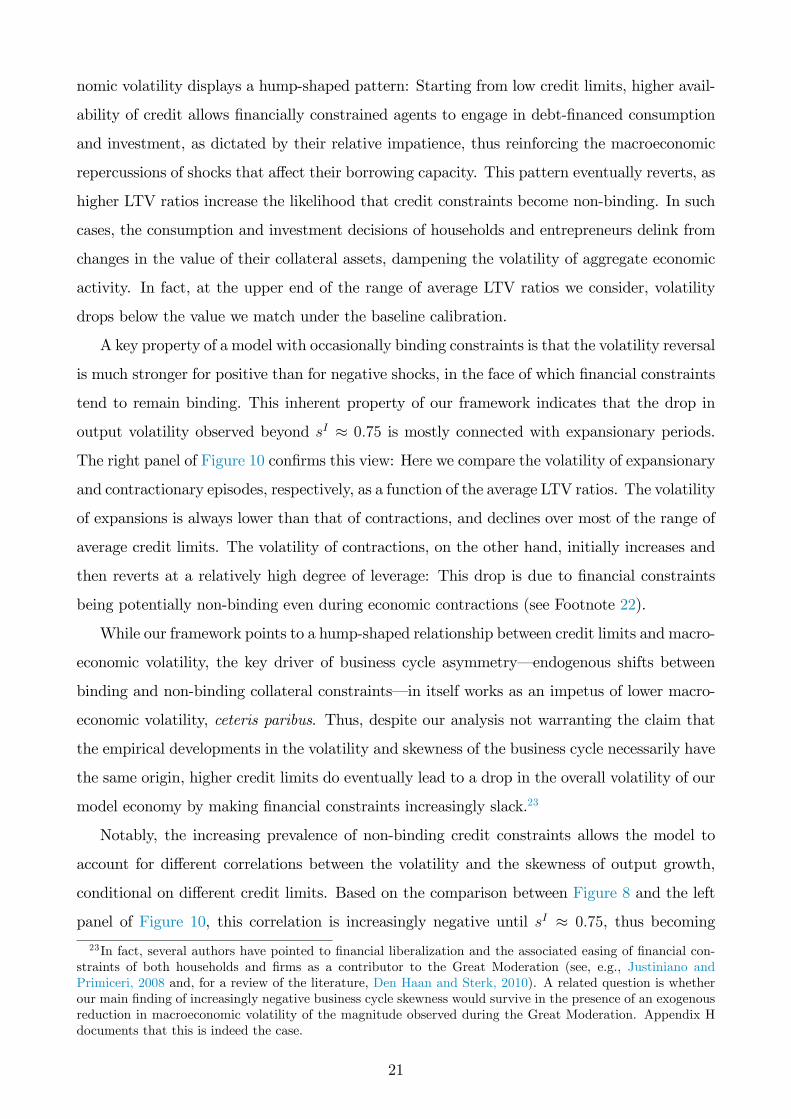
A key property of a model with occasionally binding constraints is that the volatility reversal

is much stronger for positive than for negative shocks, in the face of which financial constraints

tend to remain binding. This inherent property of our framework indicates that the drop in

output volatility observed beyond sI ≈ 0.75 is mostly connected with expansionary periods.

The right panel of Figure 10 confirms this view: Here we compare the volatility of expansionary

and contractionary episodes, respectively, as a function of the average LTV ratios. The volatility

of expansions is always lower than that of contractions, and declines over most of the range of

average credit limits. The volatility of contractions, on the other hand, initially increases and

then reverts at a relatively high degree of leverage: This drop is due to financial constraints

being potentially non-binding even during economic contractions (see Footnote 22).

While our framework points to a hump-shaped relationship between credit limits and macro-

economic volatility, the key driver of business cycle asymmetry– endogenous shifts between

binding and non-binding collateral constraints– in itself works as an impetus of lower macro-

economic volatility, ceteris paribus. Thus, despite our analysis not warranting the claim that

the empirical developments in the volatility and skewness of the business cycle necessarily have

the same origin, higher credit limits do eventually lead to a drop in the overall volatility of our

model economy by making financial constraints increasingly slack.23

Notably, the increasing prevalence of non-binding credit constraints allows the model to

account for different correlations between the volatility and the skewness of output growth,

conditional on different credit limits. Based on the comparison between Figure 8 and the left

panel of Figure 10, this correlation is increasingly negative until sI ≈ 0.75, thus becoming

23In fact, several authors have pointed to financial liberalization and the associated easing of financial con-straints of both households and firms as a contributor to the Great Moderation (see, e.g., Justiniano andPrimiceri, 2008 and, for a review of the literature, Den Haan and Sterk, 2010). A related question is whetherour main finding of increasingly negative business cycle skewness would survive in the presence of an exogenousreduction in macroeconomic volatility of the magnitude observed during the Great Moderation. Appendix Hdocuments that this is indeed the case.

21

positive as financial deepening reaches very advanced stages. These results are reminiscent

of the evidence reported by Bekaert and Popov (2015), who document a positive long-run

correlation between the volatility and skewness of output growth in a large cross-section of

countries, but also a negative short-run relationship: As financial leverage reaches a certain

level across advanced economies, our results predict that skewness and volatility will eventually

decline in conjunction.

7 Debt overhang and business cycle asymmetries

Several authors have recently pointed to the nature of the boom phase of the business cycle as

a key determinant of the subsequent recession. Using data for 14 advanced economies for the

period 1870—2008, Jordà et al. (2013) find that more credit-intensive expansions tend to be

followed by deeper recessions, whether or not the recession is accompanied by a financial crisis.

This evidence is consistent with our cross-state evidence, as well as with the results of Mian

and Sufi (2010) and Giroud and Mueller (2017), who document a strong connection between

the severity of the Great Recession and the pre-crisis leverage of households and firms at the

county level, respectively.

In this section we demonstrate that our model is also capable of reproducing these empirical

facts. Figure 11 reports the results of the following experiment: Starting in the steady state, we

generate a boom-bust cycle for different average LTV ratios. We first feed the economy with a

series of positive shocks of all three types in the first five periods (up to period 0 in the figure).

During the boom phase, we calibrate the size of the expansionary shocks hitting the economy

so as to make sure that the boom in output is identical across all the experiments. Hereafter,

starting in period 1 in the figure, we shock the economy with contractionary shocks of all three

types for two periods, after which the negative shocks are ‘phased out’over the next three

periods. Crucially, the contractionary shocks are identical across calibrations. This ensures

that the severity of the recession is solely determined by the endogenous response of the model

at each different LTV ratio.24 As the figure illustrates, the deepness of the contraction increases

with the steady-state LTV ratios. A boom of a given size is followed by a more severe recession

when debt is relatively high, as compared with the case of more scarce credit availability. At

24During both the boom and the bust we keep the relative size of the three shocks fixed and equal to theirestimated standard deviations. However, we set their persistence parameters to zero, in order to avoid that theshape of the recession may be determined by lagged values of the shocks during the boom. Finally, we makesure that impatient households and entrepreneurs remain constrained in all periods of each of the cases, so asto enhance comparability.

22

higher average LTV ratios, households and entrepreneurs are more leveraged during the boom,

and they therefore need to face a more severe process of deleveraging when the recession hits.

By contrast, when credit levels are relatively low, financially constrained agents face lower

credit availability to shift consumption and investment forward in time during booms, and are

therefore less vulnerable to contractionary shocks.

[Insert Figure 11]

We next focus on the nature of the boom and how this spills over to the ensuing contraction.

The left panel of Figure 12 compares the path of output in two different boom-bust cycles,

while the right panel shows the corresponding paths for aggregate debt. In each panel, the

dashed line represents a non-financial boom generated by a combination of technology and

land-demand shocks, while the solid line denotes a financial boom generated by credit limit

shocks.25 We calibrate the size of the expansionary shocks so as to deliver an identical increase

in output during each type of boom (which lasts for five periods, up until period 0 in the figure).

As in the previous experiment, we then subject the economy to identical sets of contractionary

shocks of all three types, so as to isolate the role played by the specific type of boom in shaping

the subsequent recession. The contractionary shocks hit in periods 1 and 2 in the figure, and

are then ‘phased out’over the next three periods. While the size of the expansion in output is

identical in each type of boom, the same is not the case for total debt, which increases by more

than twice as much during the financial boom. The consequences of this build-up of credit

show up during the subsequent contraction, which is much deeper following the financially

fueled expansion, in line with the empirical findings of Jordà et al. (2013). As in Mian and

Sufi(2010), this exercise confirms that the macroeconomic repercussions of constrained agents’

deleveraging is increasing in the size of their debt.26

[Insert Figure 12]

25In the non-financial boom we keep the relative size of the technology and land-demand shocks in line withthe values estimated in Section 5.1.2. As in the previous experiment, we set the persistence parameters of allthe shock processes to zero.26Addressing the endogeneity of credit and business cycle dynamics, Gadea-Rivas and Perez-Quiros (2015)

stress that growing credit is not a predictor of future contractions. Our model simulations are consistent withthis view. In fact, as displayed by Figure 12, output and credit growth are strongly correlated, regardless ofwhether the boom is driven by financial shocks. At the same time, the model predicts that a boom driven byfinancial shocks is associated with a stronger increase in debt and a deeper contraction, as compared with anequally-sized non-financial boom.

23

8 Concluding comments

We have documented how different dimensions of business cycle asymmetry in the US have

changed over the last few decades, and pointed to the concurrent increase in private debt as a

potential driver of these phenomena. We have presented a dynamic general equilibrium model

with credit-constrained households and firms, in which increasing leverage translates into a

more negatively skewed business cycle. This finding relies on the occasionally binding nature

of financial constraints: As their credit limits increase, households and firms are more likely to

become unconstrained during booms, while credit constraints tend to remain binding during

downturns.

These insights shed new light on the analysis of the business cycle and its developments.

The Great Moderation is widely regarded as the main development in the statistical properties

of the U.S. business cycle since the 1980s. We point to a simultaneous change in the shape of

the business cycle closely connected with financial factors. Enhanced credit access as observed

over the last few decades implies both a prolonging and a smoothing of expansionary periods

as well as less frequent– yet, relatively more dramatic– economic contractions, exacerbated

by deeper deleveraging episodes. As for the first part of this story, several contributions have

pointed to the attenuation of the upside of the business cycle as the main statistical trait of the

Great Moderation. Nevertheless, insofar as financial liberalization and enhanced credit access

can be pointed to as key drivers of an increasingly skewed business cycle, the second insight

implies that large contractionary episodes, albeit less frequent, might represent a ‘new normal’.

Our results are also of interest to macroprudential policymakers, as we complement a recent

empirical literature emphasizing that the seeds of the recession are sown during the boom (see,

e.g., Mian et al., 2017). The nature of the expansionary phase, as much as its size, is an

important determinant of the ensuing downturn, and policymakers should pay close attention

to the build-up of credit during expansions in macroeconomic activity.

24

References

Abbritti, M., and S. Fahr, 2013, Downward wage rigidity and business cycle asymmetries,

Journal of Monetary Economics, 60, 871—886.

Agca, S., and A. Mozumdar, 2008, The Impact of Capital Market Imperfections on Investment—

Cash Flow Sensitivity, Journal of Banking and Finance, 32, 207—216.

Bekaert, G., and A. Popov, 2015, On the Link between the Volatility and Skewness of Growth,

mimeo, Columbia Business School and the European Central Bank.

Brown, J. R., and B. C. Petersen, 2009, Why Has the Investment-Cash Flow Sensitivity

Declined so Sharply? Rising R&D and Equity Market Developments, Journal of Banking

and Finance, 33, 971—984.

Brunnermeier, M. K., T. Eisenbach, and Y. Sannikov, 2013, Macroeconomics with Financial

Frictions: A Survey, Advances in Economics and Econometrics, Tenth World Congress

of the Econometric Society. New York: Cambridge University Press.

Calza, A., T. Monacelli, and L. Stracca, 2013, Housing Finance and Monetary Policy, Journal

of the European Economic Association, 11, 101—122.

Campbell, J. R., and Z. Hercowitz, 2009, Welfare Implications of the Transition to High House-

hold Debt, Journal of Monetary Economics, 56, 1—16.

Chaney, T., D. Sraer, and D. Thesmar, 2012, The Collateral Channel: How Real Estate Shocks

Affect Corporate Investment, American Economic Review, 102, 2381—2409.

den Haan, W. and V. Sterk, 2010, The Myth of Financial Innovation and the Great Moderation,

Economic Journal, 121, 707—739.

Dynan, K. E., Elmendorf, D. W., and D. E. Sichel, 2006, Can Financial Innovation Help to

Explain the Reduced Volatility of Economic Activity?, Journal of Monetary Economics,

53, 123—150.

Elsby, M., B. Hobijn and A. Sahin, 2013, The Decline of the U.S. Labor Share, Brookings

Papers on Economic Activity, 44, 1—63.

Fatás, A. and I. Mihov, 2013, Recoveries, CEPR Discussion Papers, No. 9551.

25

Gadea-Rivas, M. D., A. Gomez-Loscos, and G. Perez-Quiros, 2014, The Two Greatest: Great

Recession vs. Great Moderation, CEPR Discussion Papers, No. 10092.

Gadea-Rivas, M. D., A. Gomez-Loscos, and G. Perez-Quiros, 2015, The Great Moderation in

Historical Perspective: Is it that Great?, CEPR Discussion Papers, No. 10825.

Gadea-Rivas, M. D., and G. Perez-Quiros, 2015, The Failure To Predict The Great Recession–

A View Through The Role Of Credit, Journal of the European Economic Association,

13, 534—559.

Garín, J., M. Pries, and E. Sims, 2017, The Relative Importance of Aggregate and Sectoral

Shocks and the Changing Nature of Economic Fluctuations, American Economic Journal:

Macroeconomics, forthcoming.

Gertler, M., and C. Lown, 1999, The Information in the High-Yield Bond Spread for the

Business Cycle: Evidence and Some Implications, Oxford Review of Economic Policy, 15,

132—150.

Giroud, X., and H. M. Mueller, 2017, Firm Leverage, Consumer Demand, and Unemployment

during the Great Recession, Quarterly Journal of Economics, 132, 271—316.

Graham, J. R., M. T. Leary, and M. R. Roberts, 2014, A Century of Capital Structure: The

Leveraging of Corporate America, Journal of Financial Economics, 118, 658—683.

Guerrieri, L., and M. Iacoviello, 2015, OccBin: A Toolkit for Solving Dynamic Models With

Occasionally Binding Constraints Easily, Journal of Monetary Economics, 70, 22—38.

Guerrieri, L., and M. Iacoviello, 2017, Collateral Constraints and Macroeconomic Asymmetries,

Journal of Monetary Economics, 90, 28—49.

Hamilton, J. D., 1989, A New Approach to the Economic Analysis of Nonstationary Time

Series and the Business Cycle, Econometrica, 57, 357—384.

Harding, D. and A. Pagan, 2002, Dissecting the Cycle: AMethodological Investigation, Journal

of Monetary Economics, 49, 365—381.

Herbst, E., and F. Schorfheide, 2014, Sequential Monte Carlo Sampling for DSGE Models,

Journal of Applied Econometrics, 29, 1073—1098.

Holden, T., and M. Paetz, 2012, Effi cient Simulation of DSGE Models with Inequality Con-

straints, School of Economics Discussion Papers 1612, University of Surrey.

26

Iacoviello, M., 2005, House Prices, Borrowing Constraints, and Monetary Policy in the Business

Cycle, American Economic Review, 95, 739—764.

Iacoviello, M. and S. Neri, 2010, Housing Market Spillovers: Evidence from an Estimated DSGE

Model, American Economic Journal: Macroeconomics, 2, 125—164.

Jensen, H., S. H. Ravn, and E. Santoro, 2016, Changing Credit Limits, Changing Business

Cycles, working paper, University of Copenhagen.

Jermann, U. and V. Quadrini, 2009, Financial Innovations and Macroeconomic Volatility,

working paper, Universities of Pennsylvania and Southern California.

Jermann, U. and V. Quadrini, 2012, Macroeconomic Effects of Financial Shocks, American

Economic Review, 102, 238—271.

Jordà, O., M. Schularick, and A. M. Taylor, 2013, When Credit Bites Back, Journal of Money,

Credit and Banking, 45, 3—28.

Jordà, O., M. Schularick, and A. M. Taylor, 2017, Macrofinancial History and the New Business

Cycle Facts, NBER Macroeconomics Annual 2016, 213—263.

Justiniano, A., and G. E. Primiceri, 2008, The Time Varying Volatility of Macroeconomic

Fluctuations, American Economic Review, 98, 604—641.

Justiniano, A., G. E. Primiceri, and A. Tambalotti, 2013, Is There a Trade-Offbetween Inflation

and Output Stabilization?, American Economic Journal: Macroeconomics, 5, 1—31.

Justiniano, A., G. E. Primiceri, and A. Tambalotti, 2014, Credit Supply and the Housing

Boom, working paper, Federal Reserve Bank of Chicago, Northwestern University and

Federal Reserve Bank of New York.

Justiniano, A., G. E. Primiceri, and A. Tambalotti, 2015, Household Leveraging and Delever-

aging, Review of Economic Dynamics, 18, 3—20.

Kim, C.-J. and C. R. Nelson, 1999, Has The U.S. Economy Become More Stable? A Bayesian

Approach Based On A Markov-Switching Model Of The Business Cycle, The Review of

Economics and Statistics, 81, 608—616.

Kiyotaki, N. and J. Moore, 1997, Credit Cycles, Journal of Political Economy, 105, 211—248.

27

Laséen, S., and L. E. O. Svensson, 2011, Anticipated Alternative Policy Rate Paths in Policy

Simulations, International Journal of Central Banking, 7, 1—35.

Lilliefors, H. W., 1967, On the Kolmogorov-Smirnov Test for Normality with Mean and Vari-

ance Unknown, Journal of the American Statistical Association, 62, 399—402.

Liu, Z., P. Wang, and T. Zha, 2013, Land-Price Dynamics and Macroeconomic Fluctuations,

Econometrica, 81, 1147—1184.

Maffezzoli, M., and T. Monacelli, 2015, Deleverage and Financial Fragility, CEPR Discussion

Papers, No. 10531.

Mandelman, F. S., P. Rabanal, J. F. Rubio-Ramírez, and D. Vilán, 2011, Investment-Specific

Technology Shocks and International Business Cycles: An Empirical Assessment, Review

of Economic Dynamics, 14, 136—155.

McConnell, M. M., and G. Perez-Quiros, 2000, Output Fluctuations in the United States:

What Has Changed since the Early 1980’s?, American Economic Review, 90, 1464—1476.

McKay, A., and R. Reis, 2008, The Brevity and Violence of Contractions and Expansions,

Journal of Monetary Economics, 55, 738—751.

Mendoza, E. G., 2010, Sudden Stops, Financial Crises, and Leverage, American Economic

Review, 100, 1941—1966.

Mian, A., and A. Sufi, 2010, Household Leverage and the Recession of 2007 to 2009, IMF

Economic Review, 58, 74—117.

Mian, A., A. Sufi, and E. Verner, 2017, Household Debt and Business Cycles Worldwide,

Quarterly Journal of Economics, forthcoming.

Mitchell, W. C., 1927, Business Cycles: The Problem and Its Setting, National Bureau of

Economic Research: New York.

Morley, J., and J. Piger, 2012, The Asymmetric Business Cycle, Review of Economic and

Statistics, 94, 208—221.

Neftci, S., 1984, Are Economic Time Series Asymmetric over the Business Cycle?, Journal of

Political Economy, 92, 307—328.

28

Popov, A., 2014, Credit Constraints, Equity Market Liberalization, and Growth Rate Asym-

metry, Journal of Development Economics, 107, 202—214.

Rancière, R., A. Tornell, and F. Westermann, 2008, Systemic Crises and Growth, Quarterly

Journal of Economics, 123, 359—406.

Robertson, D., A. Garratt, and S. Wright, 2006, Permanent vs. Transitory Components and

Economic Fundamentals, Journal of Applied Econometrics, 21, 521—542.

Ruge-Murcia, F., 2007, Methods to Estimate Dynamic Stochastic General Equilibrium Models,

Journal of Economic Dynamics and Control 31, 2599—2636.

Ruge-Murcia, F., 2012, Estimating Nonlinear DSGE Models by the Simulated Method of

Moments: With an Application to Business Cycles, Journal of Economic Dynamics and

Control 36, 914—938.

Sichel, D., 1993, Business Cycle Asymmetry: A Deeper Look, Economic Inquiry, 31, 224—236.

White, H., 1980, A Heteroskedasticity-Consistent Covariance Matrix and a Direct Test for

Heteroskedasticity, Econometrica, 48, 817—838.

29

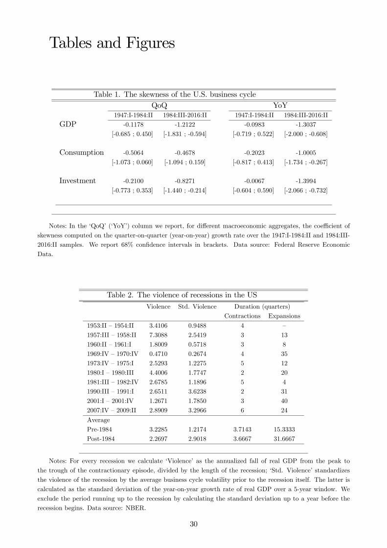
Tables and Figures

Table 1. The skewness of the U.S. business cycleQoQ YoY

1947:I-1984:II 1984:III-2016:II 1947:I-1984:II 1984:III-2016:II

GDP -0.1178 -1.2122 -0.0983 -1.3037

[-0.685 ; 0.450] [-1.831 ; -0.594] [-0.719 ; 0.522] [-2.000 ; -0.608]

Consumption -0.5064 -0.4678 -0.2023 -1.0005

[-1.073 ; 0.060] [-1.094 ; 0.159] [-0.817 ; 0.413] [-1.734 ; -0.267]

Investment -0.2100 -0.8271 -0.0067 -1.3994

[-0.773 ; 0.353] [-1.440 ; -0.214] [-0.604 ; 0.590] [-2.066 ; -0.732]

Notes: In the ‘QoQ’(‘YoY’) column we report, for different macroeconomic aggregates, the coeffi cient of

skewness computed on the quarter-on-quarter (year-on-year) growth rate over the 1947:I-1984:II and 1984:III-

2016:II samples. We report 68% confidence intervals in brackets. Data source: Federal Reserve Economic

Data.

Table 2. The violence of recessions in the US

Violence Std. Violence Duration (quarters)

Contractions Expansions

1953:II —1954:II 3.4106 0.9488 4 —

1957:III —1958:II 7.3088 2.5419 3 13

1960:II —1961:I 1.8009 0.5718 3 8

1969:IV —1970:IV 0.4710 0.2674 4 35

1973:IV —1975:I 2.5293 1.2275 5 12

1980:I —1980:III 4.4006 1.7747 2 20

1981:III —1982:IV 2.6785 1.1896 5 4

1990:III —1991:I 2.6511 3.6238 2 31

2001:I —2001:IV 1.2671 1.7850 3 40

2007:IV —2009:II 2.8909 3.2966 6 24

Average

Pre-1984 3.2285 1.2174 3.7143 15.3333

Post-1984 2.2697 2.9018 3.6667 31.6667

Notes: For every recession we calculate ‘Violence’ as the annualized fall of real GDP from the peak to

the trough of the contractionary episode, divided by the length of the recession; ‘Std. Violence’standardizes

the violence of the recession by the average business cycle volatility prior to the recession itself. The latter is

calculated as the standard deviation of the year-on-year growth rate of real GDP over a 5-year window. We

exclude the period running up to the recession by calculating the standard deviation up to a year before the

recession begins. Data source: NBER.

30

Table 3. Parameter valuesPanel A: Calibrated parameters

Parameter Description ValueβP Discount factor, patient households 0.99βi, i = I, E Discount factor, impatient households + entrepreneurs 0.96ϕi, i = P, I Curvature of utility of leisure 9νi, i = P, I Weight of labor disutility 0.27ε Weight of housing services utility 0.0763φ Non-labor input share of land 0.1340γ Labor share of production 0.6355δ Capital depreciation rate 0.0518α Income share of patient households 0.7sI Initial loan-to-value ratio, impatient households 0.6239sE Initial loan-to-value ratio, entrepreneurs 0.7139

Panel B: Estimated parametersParameter Description ValueΩ Investment adjustment cost parameter 2.9827

(0.9585)

θP Habit formation, patient households 0.0031(0.0526)

θI Habit formation, impatient households + entrepreneurs 0.7723(0.1380)

ρA Persistence of technology shock 0.9894(0.0326)

ρs Persistence of credit-limit shock 0.8873(0.0658)

ρε Persistence of land-demand shock 0.9893(0.0527)

σA Std. dev. of technology shock 0.0080(0.0012)

σs Std. dev. of credit-limit shock 0.0345(0.0011)

σε Std. dev. of land-demand shock 0.0361(0.1156)

Note: The standard errors of the estimated parameters are reported in brackets.

31

Figure 1. Growth rates of U.S. real GDP

Notes: Figure 1 reports the year-on-year rate of growth of U.S. real GDP over the 1947:I-2016:IIsample. The green bands correspond to the 68% and 90% confidence intervals from a Gaussiandensity fitted on the 1947:I-1984:II and 1984:III-2016:II samples. The vertical shadowed bandsdenote the NBER recession episodes. Data source: Federal Reserve Economic Data.

Figure 2. Household and corporate leverage in the US

Notes: Left panel: the solid-blue line graphs the ratio between loans to households and GDP, whilethe dashed-red line reports the same variable at the corporate level. Right panel: the solid-blueline graphs the ratio between households’ liabilities and assets, while the dashed-red line reportsthe same variable at the corporate level. The vertical shadowed bands denote the NBER recessionepisodes. Data source: Flow of Funds data, Financial Accounts of the US. See Appendix A fordetails.

32

Figure3.GDPgrowth:1947:I-1984:IIvs.1984:III-2016:II

Notes:Figure3reportsthehistogramofthequarter-on-quartergrowthrateofrealGDP(solid-blueline),aswellasthecorresponding

fittednormaldensity

(dotted-greenline)overthe1947:I-1984:IIand1984:III-2016:IIsamples.Datasource:FederalReserveEconomicData.

33

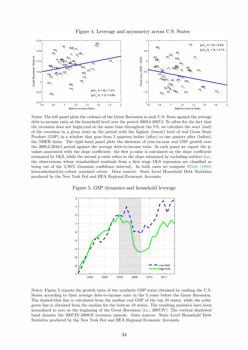
Figure 4. Leverage and asymmetry across U.S. States

Notes: The left panel plots the violence of the Great Recession in each U.S. State against the averagedebt-to-income ratio at the household level over the period 2003:I-2007:I. To allow for the fact thatthe recession does not begin/end at the same time throughout the US, we calculate the start (end)of the recession in a given state as the period with the highest (lowest) level of real Gross StateProduct (GSP) in a window that goes from 5 quarters before (after) to one quarter after (before)the NBER dates. The right-hand panel plots the skewness of year-on-year real GSP growth overthe 2005:I-2016:I period against the average debt-to-income ratio. In each panel we report the p-values associated with the slope coeffi cient: the first p-value is calculated on the slope coeffi cientestimated by OLS, while the second p-value refers to the slope estimated by excluding outliers (i.e.,the observations whose standardized residuals from a first stage OLS regression are classified asbeing out of the 5/95% Gaussian confidence interval). In both cases we compute White (1980)heteroskedasticity-robust standard errors. Data sources: State Level Household Debt Statisticsproduced by the New York Fed and BEA Regional Economic Accounts.

Figure 5. GSP dynamics and household leverage

Notes: Figure 5 reports the growth rates of two synthetic GSP series obtained by ranking the U.S.States according to their average debt-to-income ratio in the 5 years before the Great Recession.The dashed-blue line is calculated from the median real GSP of the top 10 states, while the solid-green line is obtained from the median for the bottom 10 states. The resulting statistics have beennormalized to zero at the beginning of the Great Recession (i.e., 2007:IV). The vertical shadowedband denotes the 2007:IV-2009:II recession episode. Data sources: State Level Household DebtStatistics produced by the New York Fed and BEA Regional Economic Accounts.

34

Figure 6. Impulse responses

Notes: Impulse responses of gross output (% deviation from the steady state) to a one-standarddeviation shock to technology (row 1), land demand (row 2), and credit limits (row 3). Left column:sI = 0.62, sE = 0.71; right column: sI = 0.85, sE = 0.94. The shadowed bands indicate the periodsin which the entrepreneurs are financially unconstrained.

35

Figure 7. Leverage and frequency of non-binding collateral constraints

Notes: Frequency of non-binding constraints for entrepreneurs (solid line) and impatient households(dashed line). Both statistics are graphed for different average LTV ratios faced by the impatienthousehold. Across all the simulations the entrepreneurial average LTV ratio is adjusted so as to be9 basis points greater than any value we consider for impatient households’credit limits, in line withthe baseline calibration of the model.

Figure 8. Business cycle asymmetries

Notes: Skewness of the year-on-year growth rate of output, consumption and investment (left panel),and the standardized violence of the recessions (right panel), for different average LTV ratios faced bythe impatient household. To identify the recessionary episodes in our simulated gross output series,we use the Harding and Pagan (2002) algorithm. We then compute violence as the average fall ofoutput over a given recession, divided by the length of the recession itself. Finally, we standardizeviolence by means of the volatility of year-on-year output growth over the five years prior to therecession. Across all the simulations the entrepreneurial average LTV ratio is adjusted so as to be 9basis points greater than any value we consider for impatient households’credit limits, in line withthe baseline calibration of the model.

36

Figure 9. Average duration of expansions and contractions

Notes: Duration of expansions and contractions (in quarters). To identify expansions and contrac-tions in our simulated gross output series, we use the Harding and Pagan (2002) algorithm. Theduration of both cyclical phases is graphed for different average LTV ratios faced by the impatienthousehold. Across all the simulations the entrepreneurial average LTV ratio is adjusted so as to be9 basis points greater than any value we consider for impatient households’credit limits, in line withthe baseline calibration of the model.

Figure 10. Leverage and volatility

Notes: The left panel reports the standard deviation of output growth, while the right panel reportsthe standard deviation of expansions (solid line) and contractions (dashed line) in economic activity.These are determined based on whether output is above or below its steady-state level. Across all thesimulations the entrepreneurial average LTV ratio is adjusted so as to be 9 basis points greater thanany value we consider for impatient households’credit limits, in line with the baseline calibration ofthe model.

37

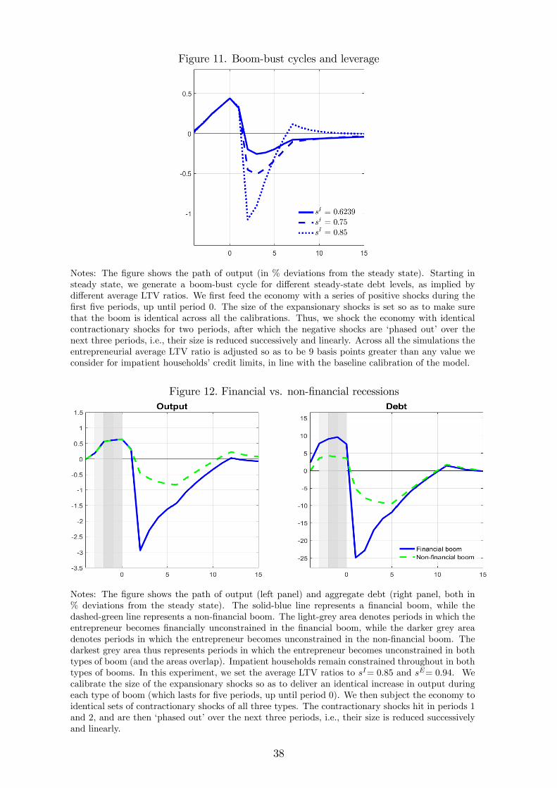
Figure 11. Boom-bust cycles and leverage

Notes: The figure shows the path of output (in % deviations from the steady state). Starting insteady state, we generate a boom-bust cycle for different steady-state debt levels, as implied bydifferent average LTV ratios. We first feed the economy with a series of positive shocks during thefirst five periods, up until period 0. The size of the expansionary shocks is set so as to make surethat the boom is identical across all the calibrations. Thus, we shock the economy with identicalcontractionary shocks for two periods, after which the negative shocks are ‘phased out’ over thenext three periods, i.e., their size is reduced successively and linearly. Across all the simulations theentrepreneurial average LTV ratio is adjusted so as to be 9 basis points greater than any value weconsider for impatient households’credit limits, in line with the baseline calibration of the model.

Figure 12. Financial vs. non-financial recessions

Notes: The figure shows the path of output (left panel) and aggregate debt (right panel, both in% deviations from the steady state). The solid-blue line represents a financial boom, while thedashed-green line represents a non-financial boom. The light-grey area denotes periods in which theentrepreneur becomes financially unconstrained in the financial boom, while the darker grey areadenotes periods in which the entrepreneur becomes unconstrained in the non-financial boom. Thedarkest grey area thus represents periods in which the entrepreneur becomes unconstrained in bothtypes of boom (and the areas overlap). Impatient households remain constrained throughout in bothtypes of booms. In this experiment, we set the average LTV ratios to sI= 0.85 and sE= 0.94. Wecalibrate the size of the expansionary shocks so as to deliver an identical increase in output duringeach type of boom (which lasts for five periods, up until period 0). We then subject the economy toidentical sets of contractionary shocks of all three types. The contractionary shocks hit in periods 1and 2, and are then ‘phased out’over the next three periods, i.e., their size is reduced successivelyand linearly.

38

Appendix A: Assets and liabilities in the US

Figure 2 shows the ratio of liabilities to assets for households and firms in the United States,respectively. All data are taken from FRED (Federal Reserve Economic Data), Federal ReserveBank of St. Louis. The primary source is Flow of Funds data from the Board of Governors ofthe Federal Reserve System. For business liabilities we use the sum of debt securities and loansof nonfinancial corporate and noncorporate businesses. For assets we follow Liu et al. (2013)and use data on both sectors’equipment and software as well as real estate at market value.For households and nonprofit organizations, we again use the sum of debt securities and loansas data for liabilities and use as assets both groups’real estate at market value and equipmentand software of nonprofit organizations.The ratios reported in Figure 2 are aggregate measures, and may therefore not reflect actual

loan-to-value (LTV) requirements for the marginal borrower. Nonetheless, we report thesefigures since the flow of funds data deliver a continuous measure of LTV ratios covering theentire period 1952—2016. For households, the aggregate ratio of credit to assets in the economyis likely to understate the actual downpayment requirements faced by households applying fora mortgage loan, since loans and assets are not evenly distributed across households. In ourmodel we distinguish between patient and impatient households, and we assume that onlythe latter group is faced with a collateral constraint. In the data we do not make such adistinction, so that the LTV ratio for households reported in Figure 2 represents an average ofthe LTV of patient households (savers), who are likely to have many assets and small loans,and that of impatient households (borrowers), who on average have larger loans and fewerassets. Justiniano et al. (2014) use the Survey of Consumer Finances and identify borrowersas households with liquid assets of a value less than two months of their income. Based on thesurveys from 1992, 1995, and 1998, they arrive at an average LTV ratio for this group of around0.8, while our measure fluctuates around 0.5 during the 1990s. Following Duca et al. (2011), analternative approach is to focus on first-time home-buyers, who are likely to fully exploit theirborrowing capacity. Using data from the American Housing Survey, these authors report LTVratios approaching 0.9 towards the end of the 1990s; reaching a peak of almost 0.95 before theonset of the recent crisis. While these alternative approaches are likely to result in higher levelsof LTV ratios, we are especially interested in the development of these ratios over a ratherlong time span. While we believe the Flow of Funds data provide the most comprehensive andconsistent time series evidence in this respect, substantial increases over time in the LTV ratiosfaced by households have been extensively documented; see, e.g., Campbell and Hercowitz(2009), Duca et al. (2011), Favilukis et al. (2017), and Boz and Mendoza (2014). It shouldbe noted that for households, various government-sponsored programs directed at lowering thedown-payment requirements faced by low-income or first-time home buyers have been enactedby different administrations (Chambers et al., 2009). These are likely to have contributed tothe increase in the ratio of loans to assets illustrated in the left panel of Figure 2.Likewise, the aggregate ratio of business loans to assets in the data may cover for a disparate

distribution of credit and assets across firms. In general, the borrowing patterns and conditionsof firms are more diffi cult to characterize than those of households, as their credit demand ismore volatile, and their assets are less uniform and often more diffi cult to assess. Liu et al.(2013) also use Flow of Funds data to calibrate the LTV ratio of the entrepreneurs, and arriveat a value of 0.75. This ratio is based on the assumption that commercial real estate enterswith a weight of 0.5 in the asset composition of firms. The secular increase in firm leverageover the second half of the 20th century has also been documented by Graham et al. (2014)

39

using data from the Compustat database.27,28 These authors report loan-to-asset ratios thatare broadly in line with those we present. More generally, an enhanced access of firms to creditmarkets over time has been extensively documented in the literature, as also discussed in themain text.

Appendix B: Additional empirical evidence

B1. Time-varying volatility and skewness

In the main text we report evidence on the skewness of real GDP growth being differentbefore and during the Great Moderation. The choice of a cut-off date is inspired by a largeliterature that has documented a drop in the volatility over the two samples. This exerciseentails a possible drawback: The estimates of the skewness can be biased by the first andsecond moment of the business cycle changing over time. In particular: i) There is now ampleevidence that the volatility of the business cycle displays a cyclical behavior (see, e.g., Kim andNelson, 1999; and McConnell and Perez-Quiros, 2000) and ii) the long-run growth rate of theeconomy since around 2000 is substantially lower than the average for the entire sample (see,e.g., Antolin-Diaz et al., 2017). To account for these issues we report a measure of time-varyingskewness of real GDP growth for the entire sample, relying on a nonparametric estimator. Tothis end, take a generic time series, yt, so that its variance and skewness can be respectivelycalculated as

σ2 = V ar (yt) =1

T

T∑t=1

(yt − µ)2 ,

% = Skew (yt) =

1

T

T∑t=1

(yt − µ)2−3/2

1

T

T∑t=1

(yt − µ)3,

where T denotes the number of observations in the sample and µ = E (yt) = T−1∑T

t=1 yt isthe sample average. Define the sample autocovariance and autocorrelation as

γτ =1

T

T−|τ |∑t=1

(yt−|τ | − µ

)(yt − µ) ,

ρτ =γτσ2.

27It should be mentioned that they also show a Flow of Funds-based measure of debt to total assets athistorical cost (or book value) for firms. The increase over time in this measure is smaller. However, we believethat the ratio of debt to pledgeable assets at market values (as shown in Figure 2) is the relevant measure forfirms’access to collateralized loans, and hence more appropriate for our purposes.28We emphasize that Figure 2 reports a gross measure of firm leverage. Bates et al. (2009) report that firm

leverage net of cash holdings has been declining since 1980, but that this decline is entirely due to a largeincrease in cash holdings.

40

When yt is a Gaussian process with absolutely summable autocovariances, it can be shownthat the standard errors associated with the two measures are:29

V ar(σ2)

=2

T

( ∞∑τ=−∞

γτ

)2,

V ar (%) =6

T

∞∑τ=−∞

ρ3τ .

In practice the two summations are truncated at some appropriate (finite) lag k.The framework we follow in order to account for time-variation in the variance and skewness

has a long pedigree in statistics, starting with the work of Priestley (1965), who introduced theconcept of slowly varying process. This work suggests that time series may have time-varyingspectral densities which change slowly over time, and proposed to describe those changes as theresult of a non-parametric process. This work has more recently been followed up by Dahlhaus(1996), as well as Kapetanios (2007) and Giraitis et al. (2014) in the context of time-varyingregression models and economic forecasting, respectively. Specifically, the time-varying varianceand skewness are calculated as

σ2t = V art (yt) =t∑

j=1

ωj,t (yj − µt)2 ,

%t = Skewt (yt) =

t∑

j=1

ωj,t (yj − µt)2

−3/2 t∑j=1

ωj,t (yj − µt)3

,

where µt =∑t

j=1 ωj,tyj. Thus, the sample moments are discounted by the function ωt,T :

ωj,t = cK

(t− jH

),

where c is an integration constant and K(T−tH

)is the kernel function determining the weight

of each observation j in the estimation at time t. This weight depends on the distance to tnormalized by the bandwidth H. Giraitis et al. (2014) show that the estimator has desirablefrequentist properties. They suggest using Gaussian kernels with the optimal bandwidth valueH = T 1/2.Similarly, we can compute the time-varying standard deviation of variance and skewness

estimates using time-varying estimates of the sample autocovariance and autocorrelations:

γτ ,t =

t−|τ |∑j=1

ωj,t(yj−|τ | − µt

)(yj − µt) ,

ρτ ,t =γτ ,tσ2t

.

Based on this, Figure B2 reports time-varying measures of volatility and skewness of GDPgrowth. The left panel confirms the widely documented decline in volatility. From the rightpanel, it is clear that skewness drops in the second subsample, with a first drop being identifiedafter the 1991 recession and a further one after the Great Recession.29The first expression computes the variance as the Newey-West variance of the squared residuals, in order

to account for the autocorrelation of the errors. The second equality follows from Gasser (1975) and Psaradakisand Sola (2003).

41

Figure B1. Time-varying volatility and skewness

Notes. Figure B1 reports the time-varying variance and skewness of year-on-year growth of realGDP (green-continuous lines)– obtained by using a nonparametric estimator in the spirit of Giraitiset al. (2014)– as well as the associated 68% confidence interval (green-dashed lines). We also reportthe variance and skewness of real GDP growth computed over the pre- and post-Great Moderationsample (blue-continuous lines), as well as the associated 68% confidence interval (blues-dashed lines).The vertical shadowed bands denote the NBER recession episodes. Sample: 1947:I-2016:II. The first10 years of data are dropped to initialize the algorithm.

B2. Normality tests

Table B2. Normality tests

GDP growth (QoQ)

1947:I-1984:II 1984:III-2016:II

KS 0.638 0.002

AD 0.534 0.000

SW 0.507 0.000

JB 0.50 0.001

GDP growth (YoY)

1947:I-1984:II 1984:III-2016:II

KS 0.289 0.004

AD 0.060 0.000

SW 0.091 0.000

JB 0.50 0.001Notes. Table B2 reports the p-values of a battery of tests assuming the null hypothesis that realGDP growth is normally distributed in a given sample. KS refers to Kolmogorov-Smirnov test withestimated parameters (see Liliefors, 1967); AD refers to the test of Anderson and Darling (1954);SW refers to the Shapiro-Wilk test (Shapiro and Wilk, 1965) with p-values calculated as outlinedby Royston (1992); JB refers to the Jarque-Bera test for normality (Jarque and Bera, 1987).

42

B3. Semivariances and asymmetry

Table B3. Semivariances

GDP growth (QoQ)

1947:I-1984:II 1984:III-2016:II

σ 4.701 2.358

σ−/σ+ 1.035 1.290

GDP growth (YoY)

1947:I-1984:II 1984:III-2016:II

σ 3.070 1.747

σ−/σ+ 1.062 1.366

Notes: Table B3 reports the volatility of different business cycle indicators and its decomposition

into upside and downside semivariance. Specifically σ =√∑T

t=1 (xt − x)2/T =

√σ2U + σ

2D, with

the upside and downside semivariance defined as σ+ =√∑T

t=1 (xt − x)21 (xt ≥ x) /T and σ− =√∑T

t=1 (xt − x)21 (xt < x) /T respectively, where 1 (z) is an indicator function taking value 1 when

condition z is true and 0 otherwise.

B4. Business cycle asymmetries across the G7 countries

In this appendix we extend the empirical analysis on evolving asymmetries in the businesscycle to the remaining G7 countries.30 To calculate asymmetry statistics for these countries, itis crucial that the underlying long-run growth is appropriately removed, as the country-specificgrowth rates display large changes over the sample under investigation (see, e.g., Antolin-Diaz et al., 2017).31 To this end, we estimate long-run growth as the first difference in thesmooth trend of the real GDP series. The latter is retrieved through the modified HP filter ofRotemberg (1999).32 We use data from 1961:II to 2016:II and split the sample in the secondquarter of 1984, so as to be consistent with the analysis in the main body of the paper.33 TableB4 reports the skewness statistics and the ratio between the (square root of the) negative andthe positive semivariance of the two subsamples for real GDP growth. For all countries wedetect a substantial fall in skewness, along with a relative increase in the negative semivariancein the post-1984 sample.

30Stock and Watson (2005) have shown that, for these countries, the mid-1980s are associated with a sharpreduction in macroeconomic volatility.31The results reported in Table 1 are robust to subtracting the underlying long-run growth rate in the US.32The non-parametric method of Rotemberg (1999) ensures that changes in trend growth are not associated

with the current stage of the cycle, thus obtaining a modicum of independence between the two series.33The results are robust to delaying the cut-off date.

43

TableB4.ChangingasymmetryfortheremainingG7countries

QoQ

YoY

Skewness

σ−/σ

+Skewness

σ−/σ

+

Pre-84

Post-84

Pre-84

Post-84

Pre-84

Post-84

Pre-84

Post-84

Canada

-0.1976

-0.9456

1.0401

1.2273

-0.9558

-1.0225

1.2835

1.3129

[-0.901;0.506]

[-1.566;-0.326]

[-1.704;-0.208][-1.717;-0.329]

France

0.3276

-0.9127

0.9680

1.1915

0.2755

-0.9043

1.0287

1.2406

[-0.367;1.022]

[-1.541;-0.284]

[-0.427;0.978]

[-1.611;-0.198]

Germany

-0.3563

-1.4303

1.0786

1.2936

-0.5077

-1.0742

1.1722

1.2213

[-1.06;0.347]

[-2.043;-0.817]

[-1.257;0.241]

[-1.757;-0.391]

Italy

0.2474

-1.1005

0.9765

1.2750

-0.4313

-1.4200

1.1425

1.4398

[-0.456;0.951]

[-1.719;-0.482]

[-1.179;0.317]

[-2.107;-0.733]

Japan

-0.5166

-0.9817

1.0854

1.2054

-0.5267

-1.0209

1.1663

1.2473

[-1.221;0.188]

[-1.594;-0.369]

[-1.299;0.246]

[-1.683;-0.358]

UnitedKingdom

0.6330

-0.9726

0.8667

1.2197

-0.4359

-1.4920

1.1484

1.4685

[-0.071;1.337]

[-1.605;-0.34]

[-1.19;0.318]

[-2.203;-0.781]

Notes:Foreachcountrythetablereportstheskewness(68%

confidenceintervalsinbrackets)andtheratioofthe(squarerootof

the)negativeoverpositivesemivariancefordetrendedGDPgrowth,1961:I-2016:II.Thedataaretakenfrom

theOECDquarterly

database.

44

B5. Additional evidence on the standardized violence of the USbusiness cycle

Table B5. Standardized violence of U.S. recessions (Robustness)

(1) (2) (3) (4) (5) (6) (7)1953:II —1954:II 0.6353 1.1270 0.7337 0.7313 0.5989 0.6644 0.5835

1957:III —1958:II 1.6292 2.4152 1.5723 1.7671 1.7163 1.6875 1.7846

1960:II —1961:I 0.3512 0.5951 0.3874 0.4288 0.3074 0.4636 0.3038

1969:IV —1970:IV 0.1631 0.1556 0.1013 0.2476 0.1548 0.2398 0.1584

1973:IV —1975:I 0.6618 0.8358 0.5441 0.8468 0.5417 0.8329 0.5086

1980:I —1980:III 0.9991 1.4542 0.9467 1.2388 0.9719 1.2342 0.8633

1981:III —1982:IV 0.5977 0.8851 0.5762 0.6452 0.4481 0.6211 0.3995

1990:III —1991:I 1.9098 1.5271 1.1319 1.3633 1.2550 1.2294 1.3007

2001:I —2001:IV 0.7295 0.7299 0.5410 0.7551 0.4630 0.7010 0.4191

2007:IV —2009:II 1.8467 1.6652 1.2343 2.0200 1.6071 1.9154 1.5710

Average

Pre-84 0.7196 1.0669 0.6945 0.8437 0.6770 0.8205 0.6574

Post-84 1.4953 1.3074 0.9691 1.3795 1.1083 1.2819 1.0969

Notes: Table B5 reports different measures of standardized violence that change depending on thebusiness cycle volatility employed in the denominator. Column (1) follows the same procedureemployed to obtain standardized violence in Table 2, though the volatility measure is retrieved fromquarter-on-quarter growth rates of real GDP. In the remaining computations, even column numbersreport violence statistics that are standardized by volatility measures retrieved from quarter-on-quarter growth rates or real GDP, while in odd column numbers the standardization is operatedthrough volatility measures obtained from year-on-year growth rates. Columns (2) and (3) calculatethe volatility by splitting the data between pre- and post-Great Moderation. In columns (4) and(5) the standardization is operated by considering the following stochastic volatility model for realGDP growth: yt = ρ0 + ρ1yt−1 + ρ2yt−2 + σtεt, where σ2t = σ2t−1 + κσ2t

(ε2t − 1

)and εt ∼ N (0, 1).

In columns (6) and (7) the standardization is operated by considering a time-varying AR model forreal GDP growth with stochastic volatility similar to that of Stock and Watson (2005), where allthe time-varying parameters follow random walk laws of motion (as in Delle Monache and Petrella,2017).

B6. Household leverage in the US

Figure B6 displays the ranking of most highly leveraged US states used in Section 2.2.

45

Figure B6. U.S. States ordered by households’average debt-to-income ratio

Notes. U.S. States ordered by the average debt-to-income ratio in the household sector, over theperiod 2003-2007.

Appendix C: Details on the solution of the two-periodmodel

Here, we provide details on the computation of the competitive equilibrium of the two-periodmodel discussed in Section 3. The notation is explained in the main text. The utility of therepresentative household is given by

E0

2∑t=1

βt−1 [a logCt + (1− a) logHt]

. (23)

The budget constraints in periods 1 and 2 are

C1 +Q1 (H1 −H0)−B1 = Y1 −RB0, (24)

C2 +Q2 (H2 −H1) = Y −RB1, (25)

respectively. The collateral constraint on debt is

B1 ≤ sE1 Q2H1

R. (26)

The model is solved by backwards induction. In period 2 the household solves

maxC2

β

a logC2 + (1− a) log

(H1 +

Y −RB1 − C2Q2

),

46

by taking as given Q2. The first-order condition is

aH2Q2 = (1− a)C2. (27)

Combined with (25), we obtain two policy functions for nondurable consumption and land:

C2 = a (Y −RB1 +Q2H1) , (28)

H2Q2 = (1− a) (Y −RB1 +Q2H1) . (29)

These provide period 2’s demand schedules as functions of the state (H1, B1), and the price Q2.Note that (28) and (29) hold for any B1, and therefore irrespective of whether the householdwas constrained or not in period 1 in its debt choice.In period 1, the individual solves

maxH1,B1

[a log [Y1 −RB0 +B1 −Q1 (H1 −H0)] + (1− a) logH1]

+β [a logC2 + (1− a) logH2] ,

s.t. (26) and (28)—(29),

taking prices Q1 and Q2 as given. The first-order conditions are

− a

C1Q1 +

1− aH1

+ β

(a

C2

∂C2∂H1

+1− aH2

∂H2

∂H1

)+ µs

Q2R

= 0, (30)

a

C1+ β

(a

C2

∂C2∂B1

+1− aH2

∂H2

∂B1

)− µ = 0, (31)

where µ ≥ 0 is the multiplier on (26) and the partial derivatives can be recovered from (28)and (29), i.e.:

∂C2∂H1

= aQ2,∂H2

∂H1

= 1− a, ∂C2∂B1

= −Ra, ∂H2

∂B1= −R (1− a)

Q2. (32)

For future reference, it is convenient to state a consolidated first-order condition found byadding (30) and (31), and applying (32):

1− aH1

+β (Q2 −Q1R)

Y −RB1 +Q2H1

= µ

(Q1 − s

Q2R

). (33)

Definition. A competitive equilibrium is a vector C1, C2, H1, H2, Q1, Q2, B1, µ, whichgiven H0, B0, Y1, and Y satisfies

(i) the first-order conditions (27), (30), (31),

(ii) the budget constraints (24), (25),

(iii) the land market-clearing conditions

H1 = H, (34)

H2 = H, (35)

where H > 0 is the exogenous stock of land,

47

(iv) the complementary slackness condition associated with (26):(B1 − s

E1 Q2H1

R

)µ = 0. (36)

In the following, we provide closed-form solutions for the variables most relevant to ouranalysis in the main text. We divide the exposition into the ‘regime’where the credit constraint(26) does not bind, µ = 0, and the one where it does, µ > 0. Then we show that it is period-1income that determines which regime prevails. We then prove that the critical income value(below which the credit constraint becomes binding) is identical to the income level that exactlymakes consumption under either regime identical. For simplicity, we let the initial stock of landequal its value in periods 1 and 2, i.e., we assume H0 = H.

The case of a non-binding credit constraint

In case of a non-binding credit constraint, we have µ = 0, and therefore (33) reduces to

1− aH1

= − β (Q2 −Q1R)

Y −RB1 +Q2H1

.

Using (34) this becomes

(1− a) (Y −RB1) + (1− a)Q2H = −βHQ2 + βRQ1H.

Combining (29) with (35) we recover

Q2 =1− aaH

(Y −RB1) . (37)

which inserted into the previous expression yields

(Y −RB1)(1− a) (1 + β)

a= βRQ1H. (38)

Then use (31) along with with µ = 0:

a

C1= −β

(a

C2

∂C2∂B1

+1− aH2

∂H2

∂B1

),

which by (32) gives

a

Y1 −RB0 +B1 −Q1 (H1 −H0)= βR

(a2

C2+

(1− a)2

H2Q2

).

Applying (34), (35) and (37) we then obtain the solution for B1:

B1 =β

1 + β(RB0 − Y1) +

1

R (1 + β)Y. (39)

Combining (39) with (38) we can recover Q1 as

Q1 =(1− a)

aH

(Y1 −RB0 +

Y

R

).

48

Consumption in period 1, in the absence of a binding credit constraint, then follows from (24)as

C1 =1

1 + β(Y1 −RB0) +

1

R (1 + β)Y, (40)

which is (3).

The case of a binding credit constraint

In the case where (26) binds, we have µ > 0 and

B1 = sQ2H1

R. (41)

By use of (34) and (37), we obtain B1 = [s (1− a) / (aR)] (Y −RB1) from which we recoverperiod-1 debt as

B1 =s (1− a)

a+ s (1− a)

Y

R. (42)

Using (42) together with the budget constraint (24), immediately gives

C1 = Y1 −RB0 +s (1− a)

a+ s (1− a)

Y

R, (43)

which is (2).

The multiplier µ and the role of Y 1It is straightforward to find the period-1 income level that equalizes nondurable consumptionunder either regime, (40) and (43). This is Y 1 as given by (4). To formally relate this value tothe question of whether the credit constraint binds or not, we derive the value of the multiplierµ ≥ 0. We have from (31) that

µ =a

C1+ β

(a

C2

∂C2∂B1

+1− aH2

∂H2

∂B1

).

Using (34), (35), (24), and applying (32), this becomes

µ =a

Y1 −RB0 +B1− βR

Y −RB1 +Q2H.

By (37) and (39), we finally get

µ =a

Y1 −RB0 +s (1− a)

a+ s (1− a)

Y

R

− aβR(1− s (1− a)

a+ s (1− a)

)Y

. (44)

Since the denominator in the first expression on the right-hand side of (44) is positive (otherwiseC1 ≤ 0), µ is strictly decreasing in Y1. We can therefore find the minimum value of Y1 thatleads to µ = 0. Call this value Y1. It then follows that for all Y1 < Y1 we have µ > 0, and for

49

all Y1 ≥ Y1, we have µ = 0. From (44) we see that Y1 satisfies

1

Y1 −RB0 +s (1− a)

a+ s (1− a)

Y

R

=βR(

1− s (1− a)

a+ s (1− a)

)Y

,

from which we recover

Y1 = RB0 +a− βs (1− a)

a+ s (1− a)

Y

βR. (45)

A comparison between (45) and (4) reveals Y1 = Y 1. Hence, as stated in the main text,Y1 ≥ Y 1 involves an unconstrained regime implying consumption given by (3). Similarly,Y1 < Y 1 characterizes the constrained regime implying that nondurable consumption is givenby (2).

Appendix D: First-order conditions of the DSGE model

This appendix reports the first-order conditions for each agent in the model.

Patient households

Patient households’optimal behavior is described by the following first-order conditions:

1

CPt − θPCP

t−1− βθP

EtCPt+1

− θPCP

t

= λPt , (46)

νP(1−NP

t

)−σPN = λPt WPt , (47)

λPt = βPRtEtλPt+1

, (48)

Qt =εt

λPt HPt

+ βPEt

λPt+1λPt

Qt+1

, (49)

where λPt is the multiplier associated with (7).

Impatient households

The first-order conditions of the impatient households are given by:

1

CIt − θICI

t−1− βθI

EtCIt+1

− θICI

t

= λIt , (50)

νI(1−N I

t

)−σIN = λItWIt , (51)

λIt − µIt = βIRtEtλIt+1

, (52)

Qt =εt

λItHIt

+ βIEt

λIt+1λIt

Qt+1

+ sIt

µItλIt

Et Qt+1Rt

, (53)

where λIt is the multiplier associated with (9), and µIt is the multiplier associated with (10).

Additionally, the complementary slackness condition

µIt

(BIt − sIt

Et Qt+1HIt

Rt

)= 0, (54)

50

must hold along with µIt ≥ 0 and (10).

Entrepreneurs

The optimal behavior of the entrepreneurs is characterized by:

1

CEt − θECE

t−1− βθE

EtCEt+1

− θECE

t

= λEt , (55)

λEt − µEt = βERtEtλEt+1

, (56)

λEt = ψEt

[1− Ω

2

(ItIt−1− 1

)2− Ω

ItIt−1

(ItIt−1− 1

)]+ βEΩEt

ψEt+1

(It+1It

)2(It+1It− 1

),

(57)

ψEt = βErKt EtλEt+1

+ βE (1− δ)Et

ψEt+1

+ µEt s

Et

EtQKt+1

Rt

, (58)

Qt = βErHt Et

λEt+1λEt

+ βEEt

λEt+1λEt

Qt+1

+ sEt

µEtλEt

Et Qt+1Rt

, (59)

where λEt , µEt and ψ

Et are the multipliers associated with (14), (15), and (16), respectively.

Moreover,

µEt

(BEt − sEt Et

QKt+1Kt +Qt+1H

Et

Rt

)= 0, (60)

holds along with µEt ≥ 0 and (16). Finally, the definition of QKt implies that

QKt = ψEt /λ

Et . (61)

Firms

The first-order conditions for the firms determine the optimal demand for the input factors:

αγYt/NPt = W P

t , (62)

(1− α) γYt/NIt = W I

t , (63)

(1− γ) (1− φ)Et Yt+1 /Kt = rKt , (64)

(1− γ)φEt Yt+1 /HEt = rHt . (65)

Appendix E: Solution method

We log-linearize the model around its non-stochastic steady state, and then solve it numericallyas described in the following. When solving the model, we treat the collateral constraints asinequalities, accounting for two complementary slackness conditions (54) and (60). We thenadopt the solution method of Holden and Paetz (2012), on which this appendix builds. Inturn, Holden and Paetz (2012) expand on previous work by Laséen and Svensson (2011). Withfirst-order perturbations, this solution method is equivalent to the piecewise linear approachdiscussed by Guerrieri and Iacoviello (2015). We have verified that their proposed solutionmethod does indeed produce identical results. Furthermore, Holden and Paetz (2012) andGuerrieri and Iacoviello (2015) evaluate the accuracy of their respective methods against aglobal solution based on projection methods. This is done for a very simple model with a

51

borrowing constraint, for which a highly accurate global solution can be obtained and usedas a benchmark. They find that the local approximations are very accurate. For the modelused in this paper, the large number of state variables (14 endogenous state variables and threeshocks) renders the use of global solution methods impractical due to the curse of dimensionalitytypically associated with such methods.The collateral constraints put an upper bound on the borrowing of each of the two con-

strained agents. While the constraints are binding in the steady state, this may not be thecase outside the steady state, where the constraints may not bind. Observe that we can re-formulate the collateral constraints in terms of restrictions on each agent’s shadow value ofborrowing; µjt , j = I, E: We know that µjt ≥ 0 if and only if the optimal debt level of agentj is exactly at or above the collateral value. In other words, we need to ensure that µjt ≥ 0. Ifthis restriction is satisfied with inequality, the constraint is binding, so the slackness conditionis satisfied. If it holds with equality, the collateral constraint becomes non-binding, but theslackness condition is still satisfied. If instead µjt < 0, agent j’s optimal level of debt is lowerthan the credit limit, so that treating his collateral constraint as an equality implies that weare forcing him to borrow ‘too much’. In this case, the slackness condition is violated. We thenneed to add shadow price shocks so as to ‘push’µjt back up until it exactly equals its lowerlimit of zero and the slackness condition is satisfied. To ensure compatibility with rationalexpectations, these shocks are added to the model as ‘news shocks’. The idea of adding suchshocks to the model derives from Laséen and Svensson (2011), who use such an approach todeal with pre-announced paths for the interest rate setting of a central bank. The contributionof Holden and Paetz (2012) is to develop a numerical method to compute the size of theseshocks that are required to obtain the desired level for a given variable in each period, and tomake this method applicable to a general class of potentially more complicated problems thanthe relatively simple experiments conducted by Laséen and Svensson (2011).We first describe how to compute impulse responses to a single generic shock, e.g., a tech-

nology shock. The first step is to add independent sets of shadow price shocks to each ofthe two log-linearized collateral constraints. To this end, we need to determine the numberof periods T in which we conjecture that the collateral constraints may be non-binding. Thisnumber may be smaller than or equal to the number of periods for which we compute impulseresponses; T ≤ T IRF . For each period t ≤ T , we then add shadow price shocks which hit theeconomy in period t but become known at period 0, that is, at the same time the economy ishit by the technology shock.Let Xt denote the log-deviation of a generic variableXt from its steady-state valueX, except

for the following variables: For the interest rates, Rt ≡ Rt−R, rHt ≡ rHt −rH and rKt ≡ rKt −rK ,and for debt, Bi

t ≡ (Bit −Bi) /Y , i = P, I, E. We can then write the log-linearized collateral

constraints, augmented with the shadow price shocks, as follows:

Y

BIBIt = sIt + Et

Qt+1

+ HI

t − βP Rt −T−1∑s=0

εSP,Is,t−s,

Y

BEBEt = sEt −βP Rt+

K

K +QHE

(EtQKt+1

+ Kt

)+

QHE

K +QHE

(EtQt+1

+ HE

t

)−T−1∑s=0

εSP,Es,t−s,

where εSP,js,t−s is the shadow price shock that hits agent j in period t = s, and is anticipated byall agents in period t = t − s = 0 ensuring consistency with rational expectations. We let allshadow price shocks be of unit magnitude. We then need to compute two sets of weights αµIand αµE to control the impact of each shock on µ

It and µ

Et . The ‘optimal’sets of weights ensure

that µIt and µEt are bounded below at exactly zero. The weights are computed by solving the

52

following quadratic programming problem:

α∗ ≡[α∗′µI α∗′µE

]′= arg min

[α′µI α′µE

] [[ µI + µI,A

µE + µE,A

]+

[µI,ε

SP,I

µI,εSP,E

µE,εSP,I

µE,εSP,E

][αµIαµE

]],

subject toα′µj ≥ 0,

µj + µj,A + µj,εSP,j

αµj + µj,εSP,k

αµk ≥ 0,

j = I, E. Here, µj and µj,A denote, respectively, the steady-state value and the unrestrictedrelative impulse response of µj to a technology shock, that is, the impulse-response of µj when

the collateral constraints are assumed to always bind. In this respect, the vector[µI + µI,A

µE + µE,A

]contains the absolute, unrestricted impulse responses of the two shadow values stacked. Further,each matrix µj,ε

SP,k

contains the relative impulse responses of µj to shadow price shocks toagent k’s constraint for j, k = I, E, in the sense that column s in µj,εSP,k represents theresponse of the shadow value to a shock εSP,js,t−s, i.e. to a shadow price shock that hits inperiod s but is anticipated at time 0, as described above.34 The off-diagonal elements of the

matrix[µI,ε

SP,I

µI,εSP,E

µE,εSP,I

µE,εSP,E

]take into account that the impatient household may be affected if

the collateral constraint of the entrepreneur becomes non-binding, and vice versa. Followingthe discussion in Holden and Paetz (2012), a suffi cient condition for the existence of a unique

solution to the optimization problem is that the matrix[µI,ε

SP,I

µI,εSP,E

µE,εSP,I

µE,εSP,E

]+

[µI,ε

SP,I

µI,εSP,E

µE,εSP,I

µE,εSP,E

]′is positive definite. We have checked and verified that this condition is in fact always satisfied.We can explain the nature of the optimization problem as follows. First, note that µj +

µj,A + µj,εSP,j

αµj + µj,εSP,k

αµk denotes the combined response of µjt to a given shock (here, a

technology shock) and a simultaneous announcement of a set of future shadow price shocksfor a given set of weights. Given the constraints of the problem, the objective is to find aset of optimal weights so that the impact of the (non-negative) shadow-price shocks is exactlylarge enough to make sure that the response of µjt is never negative. The minimization ensuresthat the impact of the shadow price shocks will never be larger than necessary to obtain this.Finally, we only allow for solutions for which the value of the objective function is zero. Thisensures that at any given horizon, positive shadow price shocks occur if and only if at least oneof the two constrained variables, µIt and µ

Et , are at their lower bound of zero in that period. As

pointed out by Holden and Paetz (2012), this can be thought of as a complementary slacknesscondition on the two inequality constraints of the optimization problem. Once we have solvedthe minimization problem, it is straightforward to compute the bounded impulse responses ofall endogenous variables by simply adding the optimally weighted shadow price shocks to theunconstrained impulse responses of the model in each period.We rely on the same method to compute dynamic simulations. In this case, however, we

need to allow for more than one type of shock. For each period t, we first generate the shockshitting the economy. We then compute the unrestricted path of the endogenous variables giventhose shocks and given the simulated values in t − 1. The unrestricted paths of the bounded

34Each matrix µj,εSP,k

needs to be a square matrix, so if the number of periods in which we guess theconstraints may be non-binding is smaller than the number of periods for which we compute impulse responses,T < T IRF , we use only the first T rows of the matrix, i.e., the upper square matrix.

53

variables (µIt and µEt ) then take the place of the impulse responses in the optimization problem.

If the unrestricted paths of µIt and µEt never hit the bounds in future periods, our simulation for

period t is fine. If the bounds are hit, we follow the method above and add anticipated shadowprice shocks for a suffi cient number of future periods. We then compute restricted values forall endogenous variables, and use these as our simulation for period t. Note that, unlike thecase for impulse responses, in our dynamic simulations not all anticipated future shadow priceshocks will eventually hit the economy, as other shocks may occur before the realization of theexpected shadow price shocks and push the restricted variables away from their bounds.

Appendix F: Data description and estimation strategy

As described in the main text, we use data for the following five macroeconomic variables ofthe U.S. economy spanning the period 1952:I—1984:II: The year-on-year growth rates (in log-differences) of real GDP, real private consumption, real non-residential investment, and realhouse prices, and the average of the deviations from trend of the two LTA series reported in theright panel of Figure 2. All data series are taken from the Federal Reserve’s FRED database,with the exception of the house price, which is provided by the US Census Bureau. The seriesare the following:

• Growth rate of Real Gross Domestic Product, billions of chained 2009 dollars, seasonallyadjusted, annual rate (FRED series name: GDPC1).

• Growth rate of Real Personal Consumption Expenditures, billions of chained 2009 dollars,seasonally adjusted, annual rate (FRED series name: PCECC96).

• Growth rate of Real private fixed investment: Nonresidential (chain-type quantity index),index 2009=100, seasonally adjusted (FRED series name: B008RA3Q086SBEA).

• Growth rate of Price Index of New Single-Family Houses Sold Including Lot Value, index2005=100, not seasonally adjusted. This series is available only from 1963:Q1 onwards.

—To obtain the house price in real terms, this series is deflated using the GDP defla-tor (Gross Domestic Product: Implicit Price Deflator, index 2009=100, seasonallyadjusted, FRED series name: GDPDEF).

• LTA data: See Appendix A. We use the average of the cyclical components– obtainedthrough a multivariate Beveridge-Nelson decomposition– of the series in the right panelof Figure 2 for the period up until 1984:II.

Estimation

We use 16 empirical moments in the SMM estimation: The standard deviations and first-orderautoregressive parameters of each of the five variables described above, the correlation of con-sumption, investment, and house prices with output, and the skewness of output, consumption,and investment. These moments are matched to their simulated counterparts from the theoret-ical model. Our estimation procedure seeks to minimize the sum of squared deviations betweenempirical and simulated moments. As some of the moments are measured in different units(e.g., standard deviations vs. correlations), we use the percentage deviation from the empiricalmoment in each case. In order for the minimization procedure to converge, it is crucial to usethe same set of shocks repeatedly, making sure that the only change in the simulated momentsfrom one iteration to the next is that arising from updating the parameter values. In practice,

54

since the list of parameter values to be estimated includes the variance of the shocks in themodel, we draw from the standard normal distribution with zero mean and unit variance, andthen scale the shocks by the variance of each of the three shock processes, allowing us to esti-mate the latter. We use a draw of 2000 realizations of each of the three shocks in the model,thus obtaining simulated moments for 2000 periods.35 To make sure that the draw of shocksused is representative of the underlying distribution, we make 501 draws of potential shockmatrices, rank these in terms of the standard deviations of each of the three shocks, and selectthe shock matrix closest to the median along all three dimensions. This matrix of shocks is thenused in the estimation. In the estimation, we impose only very general bounds on parametervalues: All parameters are bounded below at zero, and the habit formation parameters alongwith all AR(1)-coeffi cients are bounded above at 0.99– a bound that is never attained.To initiate the estimation procedure a set of initial values for the estimated parameters are

needed. These are chosen based on values reported in the existing literature. It is importantto state that the estimation results proved robust to changes in the set of initial values, as longas these remain within the range of available estimates. Based on the empirical estimates ofJustiniano et al. (2013), we set the initial values of the investment adjustment cost parameter(Ω) and the parameters governing habit formation in consumption for the three agents to 4and 0.7, respectively.36 For the technology shock, we choose values similar to those used inmost of the real business cycle literature, ρA = 0.97 and σA = 0.005 (see, e.g., Mandelman etal., 2011). For the credit limit shock, we set the persistence parameter ρs = 0.98, while thestandard deviation is set to σs = 0.01, consistent with the values estimated by Jermann andQuadrini (2012) and Liu et al. (2013). Finally, for the land-demand shock, we set ρε = 0.96and σε = 0.06, in line with Iacoviello and Neri (2010) and Liu et al. (2013).We abstain from using an optimal weighting matrix in the estimation. This choice is based

on the findings of Altonji and Segal (1996), who show that when GMM is used to estimatecovariance structures and, potentially, higher-order moments such as variances, as in our case,the use of an optimal weighting matrix causes a severe downward bias in estimated parametervalues. Similar concerns apply to SMM as to GMM. The bias arises because the momentsused to fit the model itself are correlated with the weighting matrix, and may thus be avoidedby the use of fixed weights in the minimization. Altonji and Segal (1996) demonstrate thatminimization schemes with fixed weights clearly dominate optimally weighted ones in suchcircumstances. Ruge-Murcia (2012) points out that parameter estimates remain consistentfor any positive-definite weighting matrix, and finds that the accuracy and effi ciency gainsassociated with an optimal weighting matrix are not overwhelming. The empirical momentsand their model counterparts upon estimation are reported in Table F1.When computing standard errors, we rely on a version of the delta method, as described,

e.g., in Hamilton (1994). We approximate the numerical derivative of the moments with respectto the estimated parameters using the secant that can be computed by adding and subtractingε to/from the estimates, where ε is a very small number. The covariance (or spectral density)matrix is estimated using the Newey-West estimator.

35Our simulated sample is thus more than 15 times longer than the actual dataset (which spans 130 quarters).Ruge-Murcia (2012) finds that SMM is already quite accurate when the simulated sample is five or ten timeslonger than the actual data.36Unlike the other estimated parameters, θP and θI also affect the steady state of the model. To account

for this, we rely on the following iterative procedure: We first calibrate the model based on the starting valuefor θP and θI . Upon estimation, but before simulating the model, we recalibrate it for the estimated values ofthe habit parameters. This leads only to a small change in the value of ε, while the remaining parameters areunaffected.

55

Table F1. Empirical and simulated moments

Model simulations U.S. data (1952:I—1984:II)Standard deviations (percent)

Output 2.75 2.84Consumption 2.00 2.23Investment 6.25 6.91House price 3.71 3.05LTV ratio 7.46 6.96

SkewnessOutput −0.16 −0.38Consumption −0.17 −0.31Investment −0.07 −0.41

AutocorrelationsOutput 0.78 0.82Consumption 0.58 0.81Investment 0.89 0.84House price 0.61 0.79LTV ratio 0.89 0.92

Correlations with outputConsumption 0.93 0.85Investment 0.92 0.75House price 0.66 0.38

56

Appendix G: Impulse-responses

Figure G1. Impulse responses to a Technology Shock

Notes: Impulse responses of key macroeconomic variables (% deviation from the steady state) toa one-standard deviation shock to technology. Left column: sI = 0.62, sE = 0.71; right column:sI = 0.85, sE = 0.94. The shadowed bands indicate the periods in which the entrepreneurs arefinancially unconstrained.

57

Figure G2. Impulse responses to a Land Demand Shock

Notes: Impulse responses of key macroeconomic variables (% deviation from the steady state) to aone-standard deviation shock to land demand. Left column: sI = 0.62, sE = 0.71; right column:sI = 0.85, sE = 0.94. The shadowed bands indicate the periods in which the entrepreneurs arefinancially unconstrained.

58

Figure G3. Impulse responses to a Credit Limit Shock

Notes: Impulse responses of key macroeconomic variables (% deviation from the steady state) toa one-standard deviation shock to credit limit. Left column: sI = 0.62, sE = 0.71; right column:sI = 0.85, sE = 0.94. The shadowed bands indicate the periods in which the entrepreneurs arefinancially unconstrained.

Appendix H: Skewness and the Great Moderation

In the main text, we demonstrated that our model was able to generate a more negativelyskewed business cycle along with a drop in macroeconomic volatility when we raise the steady-state LTV ratios. However, the drop in the standard deviation of GDP growth documented inFigure 10 falls short of the decline observed in US data during the Great Moderation period. Inthis respect, it is important to recognize that none of the factors to which the Great Moderationis typically ascribed are featured in our model. One widely cited explanation for the GreatModeration is the so-called ‘Good Luck’hypothesis, according to which the Great Moderationwas simply a result of smaller shocks hitting the US economy (see, e.g., Stock and Watson,2003).37 The goal of this appendix is to demonstrate that our main finding of an increasinglynegatively skewed business cycle holds up in an environment where increasing LTV ratios arecombined with smaller macroeconomic shocks to obtain a drop in output volatility similar to

37Other popular explanations include better monetary policy (Boivin and Giannoni, 2006) and smaller de-pendence on oil (Nakov and Pescatori, 2010).

59

that observed in the data. It is important to stress that this coexistence is not trivial: All elseequal, reducing the size of the shocks hitting the economy lowers the probability that collateralconstraints become non-binding, thus potentially weakening the key driver of business cycleskewness in our model.The Great Moderation entailed a decline in the volatility of GDP growth in the US economy

of around 40%, see Section 2.1. In the following, we engineer a similar decline in outputvolatility in our model simulations by reducing the standard deviations of all three shocks inthe model, keeping their relative size fixed in accordance with the estimation in Section 5.1.2.To obtain the desired drop in the volatility of GDP growth at sI = 0.90, we need to reduce thestandard deviation of each shock by 30%. We first assume that the decline in the size of theshocks occurred gradually along with the increase in LTV ratios. The top row of Figure H1shows the pattern of the standard deviation and skewness of GDP growth in this experiment.The right panel illustrates that in this case, the drop in macroeconomic volatility is similar tothat observed in the data during the Great Moderation, as desired. In addition, in contrastto the results reported in Section 6.3, the standard deviation of output growth now declinesmonotonically. The left panel shows that the decline in skewness of GDP growth survives in thisenvironment. In fact, the magnitude of the drop in skewness is almost identical to the baselineresults presented in Section 6.2 of the main text. This demonstrates that the mechanism givingrise to business cycle skewness in our model is compatible with the Good Luck hypothesis ofthe decline in macroeconomic volatility observed during the Great Moderation.Some may argue that the Great Moderation entailed a discrete, downward shift in the size

of macroeconomic shocks hitting the US economy rather than the gradual decline assumedabove. The bottom row of Figure H1 shows the results from an experiment in which thestandard deviation of each shock is reduced by 30% starting at sI = 0.6239, and then keptat this new level as the LTV ratios are increased. By design, the standard deviation of GDPgrowth reaches the same level as in the top row of Figure H1 when sI = 0.90. The hump-shapedpattern of output volatility presented in Section 6.3 is preserved in this experiment, though ata lower level. Importantly, skewness of GDP growth displays roughly the same pattern as inthe top row, confirming again the robustness of our main finding.

60

Figure H1. Skewness and the Great Moderation

Notes. The top row displays the skewness and standard deviation of output growth in the experimentwhere the size of shocks is reduced gradually, while the bottom row displays the same statistics inthe case where the size of shocks is reduced at once. In each case, the numbers reported are medianvalues from 501 stochastic model simulations of 2000 periods each.

References

Altonji, J. G., and L. M. Segal, 1996, Small-Sample Bias in GMM Estimation of CovarianceStructures, Journal of Business and Economic Statistics 14, 353—366.

Anderson, T. W. and D. A. Darling, 1954, A Test of Goodness-of-Fit, Journal of the AmericanStatistical Association, 49, 765—769.

Antolin-Diaz, J., T. Drechsel, and I. Petrella, 2017, Tracking the Slowdown in Long-Run GDPGrowth, Review of Economics and Statistics, forthcoming.

Bates, T. W., K. M. Kahle, and R. M. Stulz, 2009, Why Do U.S. Firms Hold So Much MoreCash than They Used To?, Journal of Finance, 64, 1985—2021.

Boivin, J., and M. Giannoni, 2006, Has Monetary Policy Become More Effective?, Review ofEconomics and Statistics, 88, 445—462.

Boz, E., and E. Mendoza, 2014, Financial Innovation, the Discovery of Risk, and the U.S.Credit Crisis, Journal of Monetary Economics, 62, 1—22.

Chambers, M., C. Garriga, and D. Schlagenhauf, 2009, Accounting for Changes in the Home-ownership Rate, International Economic Review, 50, 677—726.

Dahlhaus, R., 1996, Fitting time series model to nonstationary processes, Annals of Statistics,25, 1—37.

61

Delle Monache, D. and I. Petrella, 2017, Adaptive Models and Heavy Tails with an Applicationto Inflation Forecasting, International Journal of Forecasting, 33, 482—501.

Duca, J. V., J. Muellbauer, and A. Murphy, 2011, House Prices and Credit Constraints: MakingSense of the U.S. Experience, Economic Journal, 121, 533—551.

Favilukis, J., S. C. Ludvigson, and S. Van Nieuwerburgh, 2017, The Macroeconomic Effectsof Housing Wealth, Housing Finance, and Limited Risk-Sharing in General Equilibrium,Journal of Political Economy, 125, 140—223.

Gasser, T., 1975, Goodness-of-fit Tests for Correlated Data, Biometrika, 62, 563—570.

Giraitis, L., Kapetanios, G., and Yates, T., 2014, Inference on stochastic time-varying coeffi -cient models, Journal of Econometrics, 179, 46—65.

Hamilton, J. D., 1994, Time Series Analysis, Princeton University Press, Princeton, NJ.

Jarque, C., and A. Bera, 1987, A Test for Normality of Observations and Regression Residuals,International Statistical Review, 55, 163—172.

Kapetanios, G., 2007, Estimating deterministically time-varying variances in regression models,Economics Letters, 97, 97—104.

Nakov, A., and A. Pescatori, 2010, Oil and the Great Moderation, Economic Journal, 120,131—156.

Priestley, M., 1965, Evolutionary spectra and nonstationary processes, Journal of the RoyalStatistical Society, Series B, 27, 204—37.

Psaradakis, Z., and M. Sola, 2003, On Detrending and Cyclical Asymmetry, Journal of AppliedEconometrics, 18, 271—289.

Rotemberg, J. J., 1999, A Heuristic Method for Extracting Smooth Trends from EconomicTime Series, NBER Working Papers 7439, National Bureau of Economic Research.

Royston, P., 1992, Approximating the Shapiro-Wilk W-test for Non-normality, Statistics andComputing, 2, 117—119.

Shapiro, S., and M. Wilk, 1965, An Analysis of Variance Test for Normality (Complete Sam-ples), Biometrika, 52, 591—611.

Stock, J., and M. Watson, 2003, Has the Business Cycle Changed and Why?, NBER Macro-economics Annual 2002, 159—230.

Stock, J., and M. Watson, 2005, Understanding Changes In International Business Cycle Dy-namics, Journal of the European Economic Association, 3, 968—1006.

62