The Influence of the Binder Type & Aggregate Nature on the ...

The Influence of the Binder Type & Aggregate Nature on the

Electrical Resistivity and Compressive Strength of Conventional

Concrete

Hugo Deda

A thesis submitted to the University of Ottawa in partial fulfillment of the requirements for

the degree of

MASTER OF APPLIED SCIENCE

in Civil Engineering

Department of Civil Engineering

Faculty of Engineering

University of Ottawa

© Hugo Deda, Ottawa, Canada, 2020

ii

Abstract

Concrete has been used in a number of civil engineering applications due to its interesting

fresh, hardened, and durability-related properties. 28-day compressive strength is the most

important hardened state property and is frequently used as an indicator of the material’s

quality. However, early-age mechanical properties are a key factor nowadays to enhance

construction planning. Several advanced techniques have been proposed to appraise

concrete microstructure and quality, and among those electrical resistivity (ER) is one of the

most commonly used since it is a non-destructive and low-cost technique. Although recent

literature data have shown that ER may be significantly influenced by a variety of parameters

such as the test setup, material porosity and moisture content, binder type/amount and

presence of supplementary cementing materials (SCMs) along with the nature of the

aggregates used in the mix, further research must be performed to clarify the influence of

the raw materials (i.e. SCMs and aggregate nature) on ER using distinct setups. Therefore,

this work aims to appraise the influence of the coarse aggregate nature and binder

replacement/amount on the concrete ER and compressive strength predictions models

through ER. Twenty-four concrete mixtures were developed with two different coarse

aggregate natures (i.e. granite and limestone), two different water-to-binder ratios (w/b; i.e.

0.6 and 0.4) and incorporating two different SCMs (i.e. slag and fly-ash class F) with different

replacement levels. Moreover, three distinct ER techniques (e.g. bulk, surface, and internal)

and compressive strength tests were performed at different ages (i.e. 3, 7, 14, and 28 days).

Results indicate that the binder type and replacement amount significantly affect ER and

compressive strength. Otherwise, the coarse aggregate nature presented only trivial

influence for 0.6 w/b mixes, except for 50% fly-ash replacement samples; whereas for

concrete specimens with enhanced microstructure (i.e. 0.4 w/b), the aggregate nature

influence was statically significant especially for the binary mixtures with high SCMs

replacement levels (i.e. 70% GGBS and 50% fly-ash). Finally, all ER test setups were

considered to be quite suitable and reliable NDT techniques correlating themselves very

iii

well. Yet the internal resistivity setup demonstrated to be the device which yields the lowest

variability amongst them.

Keywords:. Electrical resistivity, non-destructive testing, concrete microstructure,

supplementary cementitious materials.

iv

Acknowledgements

I would like to express my deepest gratitude to two professors that were essential on my

journey during this whole Master process until the present day. First of all, I will always be

thankful to Dr. Leandro Sanchez for all the support and guidance during my Master's course

here at the University of Ottawa. Dr. Sanchez was not only an example of a top-notch

professional that will always be a reference in my career but professor Sanchez was also a

great friend in my personal life that taught me very important lessons that I will always bring

to my life. I also would like to thank Professor Sandra Dórea from UFS that believed in my

potential to accomplish this international program since the first time we met. Moreover,

Professor Sandra also did an amazing role as mental health mentor providing precious advice

during my whole passage in cold lands.

The support of my parents, Denise and Hylton, and my brothers. To my mother for always

being present, especially for all the support during COVID-19 pandemic, and for believing in

my potential even more than me. My father, for showing me the engineering life perspective

since I was a child and always teach me that nothing in life comes without giving your best.

My deepest thanks to my wife Nathalia Monteiro who helped me since my first semester in

my undergrad to the submission of this work. I will always be grateful for all of her support

during presentations, writing, and exam periods.

The efforts of my lab colleagues that help me all from material collection to the most

profound discussions about concrete. I would like to express my gratitude to Bryan Serrano,

Cassandra Trottier, Diego Souza, Luan Antunes, and Laiba Khan for all the help during my

sample fabrication and management of samples required to do this thesis. I also would like

to acknowledge all the help that Mayra de Grazia dedicated during my Master's course.

Mayra revealed to be one of the most hard-working and positive professionals that I ever

met. I would like to extremely thank MASc. Sarah Decarufel from Giatec Scientific Inc. for all

the prompt support and all the help Sarah and Giatec`s team provided during this research

project. I feel blessed to have the opportunity to work with each and every one of you.

v

I would like to acknowledge the lab technician at the University of Ottawa, Muslim Majeed,

and Gamal Elnabelsya, for teaching and helping with all daily tasks.

Last but not least, I would like to extremely thank Natural Sciences and Engineering Research

Council of Canada (NSERC) for the funding they provided for this research project.

vi

Table of Contents

Abstract ……………………………………………………………………………………………………………………………. ii

Table of Contentsm………………………………………………………………………………………………………….. vi

List of Figures……………………………………………………………………………………………………………………. ix

List of Tables…………………………………………………………………………………………………………………….. xi

List of Symbols/Abbreviations…………………………………………………………………………………………. xii

1. Chapter One: Introduction .................................................................................................1

1.1. Importance of concrete early-age compressive strength ....................................1

1.2. Research Objectives ..............................................................................................2

1.3. Thesis Organization ...............................................................................................2

1.4. References ............................................................................................................3

2. Chapter Two: Background and Literature Review .............................................................5

2.1. Non-destructives techniques ................................................................................5

2.1.1. Swiss hammer .......................................................................................................5

2.1.2. Ultrasonic pulse velocity .......................................................................................6

2.1.3. Concrete electrical resistivity ................................................................................6

2.1.3.1. Test Setups ............................................................................................................7

2.1.3.2. Overview ...............................................................................................................8

2.1.3.3. Impact of external factors on concrete ER .........................................................10

2.1.3.4. Impact of internal factors on concrete ER ..........................................................13

2.1.4. Determination of compressive strength through ER. .........................................25

2.2. Science gap .........................................................................................................27

2.3. References ..........................................................................................................28

3. Chapter Three: The Influence of the Binder Type & Aggregate Nature on the Electrical Resistivity of Conventional Concrete .....................................................................................33

3.1. Introduction ........................................................................................................34

3.2. Background .........................................................................................................35

3.2.1. Influence of external factors on concrete ER .....................................................35

3.2.2. Influence of internal factors on concrete ER ......................................................36

3.2.3. Compressive strength prediction........................................................................37

3.3. Scope of Work .....................................................................................................38

3.4. Materials and methods .......................................................................................38

vii

3.4.1. Testing procedures .............................................................................................40

3.4.1.1. Two points uniaxial technique (Bulk ER) ............................................................40

3.4.1.2. Wenner four-points technique (Surface ER).......................................................41

3.4.1.3. Internal ER ...........................................................................................................41

3.4.2. Samples fabrication ............................................................................................42

3.5. Results .................................................................................................................42

3.5.1. Electrical Resistivity.............................................................................................42

3.5.2. Compressive strength .........................................................................................47

3.6. Discussion ...........................................................................................................48

3.6.1. Influence of the test setup on ER results ............................................................48

3.6.2. Influence of raw materials on ER results ............................................................51

3.6.2.1. Influence of coarse aggregate nature on concrete ER .......................................51

3.6.2.2. Influence of binder type on concrete ER ............................................................53

3.6.3. Forecasting compressive strength through the use of ER ..................................54

3.6.3.1. Influence of binder type on concrete ER ............................................................57

3.7. Conclsuions .........................................................................................................58

3.8. References ..........................................................................................................59

4. Chapter Four: Conclusion and future recommendations ................................................64

5. Chapter Five: Appendix ....................................................................................................66

5.1. Introduction ........................................................................................................66

5.2. Materials and Methods .......................................................................................66

5.2.1. Porosity test ........................................................................................................66

5.2.2. Fresh state pore solution extraction...................................................................67

5.2.3. Pore Solution ICP-ES analysis ..............................................................................68

5.3. Results .................................................................................................................68

5.3.1. Apparent Porosity ...............................................................................................68

5.3.2. Pore Solution ER and pH .....................................................................................69

5.3.3. ICP-ES ..................................................................................................................70

5.4. Discussion ...........................................................................................................72

5.4.1. Apparent Porosity ...............................................................................................72

5.4.2. SCM replacement influence on pastes Pore Solution ........................................72

5.5. Conclusion ...........................................................................................................74

viii

5.6. References ..........................................................................................................74

ix

List of Figures

Figure 2.1. Swiss Hammer schematic. ..................................................................................... 5

Figure 2.2. Ultrasonic Pulse velocity method schematic. ....................................................... 6

Figure 2.3. Electrical resistivity measuring techniques: a) four-point method; b) two-point uniaxial method; c) internal ER sensor setup. ......................................................................... 8

Figure 2.4. RCPT and surface ER relationship: a) at 28 days; b) at 91 days . .......................... 9

Figure 2.5. Relative Humidity effect on concrete ER. ........................................................... 11

Figure 2.6. Temperature effect on concrete ER. ................................................................... 12

Figure 2.7. Sensitivity to temperature influence based on degree of saturation ................. 12

Figure 2.8. Signal frequency influence on concrete ER. ........................................................ 12

Figure 2.9. Simplified conductivity concrete model proposed by Ping et al......................... 13

Figure 2.10. Possible electrical percolation paths. ................................................................ 14

Figure 2.11. Volume of aggregate influence on concrete ER. ............................................... 14

Figure 2.12. Volume of aggregate influence on mortar ER. .................................................. 15

Figure 2.13. Concrete normalized electrical conductivity over time varying aggregate volumes . ............................................................................................................................... 15

Figure 2.14. Relationship between concrete compressive strength and conductivity for different aggregate volumes. ................................................................................................ 16

Figure 2.15. Aggregate size influence on concrete ER. ......................................................... 17

Figure 2.16. Aggregate type influence on concrete ER. ........................................................ 17

Figure 2.17. Coarse aggregate influence on concrete ER control mixes: a) 0.40 w/c; b) 0.45 w/c; c) 0.50 w/c . ................................................................................................................... 19

Figure 2.18. Coarse aggregate influence on concrete ER 20% fly ash replacement: a) 0.40 w/c; b) 0.45 w/c; c) 0.50 w/c. ................................................................................................ 19

Figure 2.19. Paste resistivity evolution over-time from paste mixtures 1 to 4 together with 8 . .......................................................................................................................................... 21

Figure 2.20. Paste resistivity evolution over-time from paste mixtures 5 to 8. ................... 21

Figure 2.21. Porlandite consumption for 10% dosage. ......................................................... 21

Figure 2.22. Conductivity evolution over-time. .................................................................... 22

Figure 2.23. Conductivity evolution over-time for 0.40 w/c samples. .................................. 23

Figure 2.24. Paste bulk Electrical Resistivity and pore solution electrical resistivity alkali content influence with (a) 0.37 w/c ratio pastes; and (b) 0.50 w/c ratio pastes.................. 24

Figure 2.25. Non-contact Electrical Resistivity meter device schematic. ............................. 25

Figure 2.26. Concrete w/c ratio versus Electrical Resistivity for different ages. .................. 25

Figure 2.27. Submerged Electrical Resistivity meter. ............................................................ 26

Figure 2.28. Relationship between w/c and concrete ER: a) control concrete samples; b) class-F fly-ash mixtures. ........................................................................................................ 26

Figure 2.29. Compressive strength and concrete ER relationship: a) 0.5 w/c mixtures; b) 0.4 w/c mixtures. ......................................................................................................................... 27

Figure 3.1. Coarse Aggregate: a) Granite; b) Limestone. ...................................................... 39

Figure 3.2. Electrical resistivity measuring techniques: a) two-point uniaxial method; b) four-point method. ................................................................................................................ 41

x

Figure 3.3. Internal ER sensor setup...................................................................................... 42

Figure 3.3. Surface ER outcomes: a) 0.6 w/b GGBS and ternary mixtures; b) 0.4 w/b GGBS and ternary mixtures; c) 0.6 w/b fly ash mixtures; d) 0.4 w/b fly ash mixtures. .................. 43

Figure 3.4. Bulk ER progression: a) 0.6 w/b GGBS and ternary mixtures; b) 0.4 w/b GGBS and ternary mixtures; c) 0.6 w/b fly ash mixtures; d) 0.4 w/b fly ash mixtures. .................. 45

Figure 3.5. Internal ER growth: a) 0.6 w/b GGBS and ternary mixtures; b) 0.4 w/b GGBS and ternary mixtures; c) 0.6 w/b fly ash mixtures; d) 0.4 w/b fly ash mixtures. ......................... 46

Figure 3.6. Compressive strength development: a) 0.6 w/b mixtures; b) 0.4 w/b mixtures.47

Figure 3.7. Setup relationships a) Surface versus Bulk ER 0.6 w/b mixtures; b) Surface versus Bulk ER 0.4 w/b mixtures; c) Internal ER versus Surface ER 0.6 w/b mixtures; d) Internal ER versus Surface ER 0.4 w/b mixtures; e) Internal ER versus Bulk ER 0.6 w/b mixtures; f) Internal ER versus Bulk ER 0.4 w/b mixtures. .................................................... 50

Figure 3.8. Hypothetical Internal ER evolution: a) 0.6 w/b mixtures; b) 0.4 w/b mixtures. 51

Figure 3.9. Relationship between compressive strength and surface (a) 0.6 w/b mixtures and b) 0.4 w/b mixtures; and internal ER (c) 0.6 w/b mixtures and d) 0.4 w/b mixture) used to determine logarithm parameters. .................................................................................... 55

Figure 3.10. Analysis of experimental-to-predicted compressive strength ratio predicted through surface ER: a) 0.6 w/b mixtures; b) 0.4 w/b mixtures. ............................................ 57

Figure 3.11. Experimental-to-predicted compressive strength ratio predicted through internal ER: a) 0.6 w/b mixtures; b) 0.4 w/b mixtures. ......................................................... 58

Figure 5.1. a) Samples Cutting Scheme; b) Porosity Test Setup. .......................................... 67

Figure 5.2. Fresh state pore solution extraction setup. ........................................................ 67

Figure 5.3. Apparent Porosity Fresh at 28 days outcomes: a) 0.6 w/b mixtures; b) 0.4 w/b mixtures. ................................................................................................................................ 68

Figure 5.4. Pores Solution ionic composition in percentage: a) 0.6 w/b mixtures; b) 0.4 w/b mixtures. ................................................................................................................................ 70

Figure 5.5. Ca2+/(k++ Na+) ratio and OH- ion concentration correlation. ............................. 73

Figure 5.6. Relationship between Pore Solution ER and OH- concentration. ...................... 73

xi

List of Tables

Table 2.1. Electrical Resistivity measurements to analyze chloride penetration on slabs. .... 9

Table 2.2. Relationship between RCPT at 56-day and surface ER at 28 day. ........................ 10

Table 2.3. Influence of aggregate size and type on Electrical Resistivity geometrical factor. ............................................................................................................................................... 16

Table 2.4 Rock electrical resistivity by rock lithotype ........................................................... 18

Table 2.5. Paste specifications. ............................................................................................. 20

Table 2.6. Mortar mix-proportions ....................................................................................... 22

Table 2.7. Fresh pore solution and pastes ER. ...................................................................... 23

Table 3.1. Aggregates characterization. ................................................................................ 39

Table 3.2. Concrete mixture proportions. ............................................................................. 40

Table 3.3. Binder’s chemical composition and density. ........................................................ 40

Table 3.4. Experimental ratios between ER setups. .............................................................. 48

Table 3.5. Statistical analysis 0.6 and 0.4 w/b samples to appraise the difference of aggregate nature in the surface and bulk ER. ....................................................................... 52

Table 3.6. Regression parameters. ........................................................................................ 56

Table 5.1. Pastes Pore Solution ER and pH ........................................................................... 69 Table 5.2. Pastes Pore Solution ionic composition in mol/L .................................................71

xii

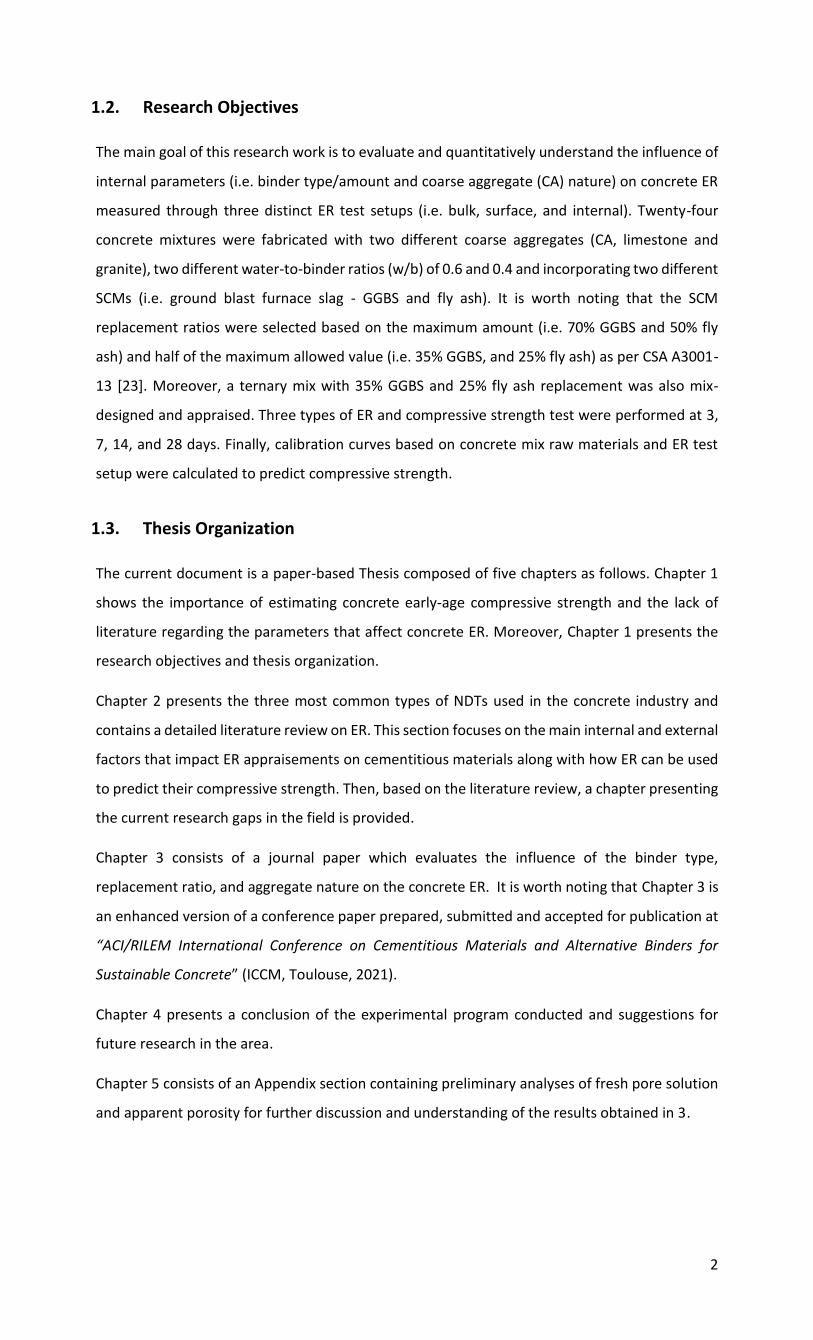
List of Symbols/Abbreviations

a Surface electrical resistivity probe spacing distance

AC Alternating current

ANOVA Analysis of variance

AASHTO American Association of State Highway and Transportation Officials

b Logarithm regression slope constant

BSE Back scattered electron

c Logarithm regression interception constant

Cp Pulse velocity

CA Coarse aggregate

COV Coefficient of variance

C-S-H Calcium silicate hydrate

d Concrete density

E Concrete static modulus of elasticity

ER Electrical resistivity

F Fly-ash

G Granite coarse aggregate

GGBS Ground granulated blast-furnace slag

I Toroidal current

i Alternating current

ITZ Interfacial transition zone

L Limestone coarse aggregate

K Electrical resistivity geometrical factor

Kbulk Bulk electrical resistivity geometrical factor

Ksurface Surface electrical resistivity geometrical factor

θ Interfacial excess conductance

MK Metakaolin

MS Micro-silica

NDT Non destructive technique

PC Portland cement

PSD Particle size distribution

P-wave Pulse velocity

ρ Electrical resistivity

ρbulk Bulk electrical resistivity

ρinternal Internal electrical resistivity

xiii

ρsurface Surface electrical resistivity

R River rock

RCPT Rapid Chloride Permeability Test

RH Relative Humanity

Rc Concrete electrical resistance

Ro Electrical resistance

RN Rebound number

SCM Supplementary cementing materials

SD Standard deviation

SF Ternary mixtures containing slag and fly-ash

UPV Ultrasonic pulse velocity

V Electrical potential

ν Poisson`s ratio

Vf,sand Sand volume fraction

w/c Water-to-cement ratio

w/b Water-to-binder ratio

γ Dimensionless surface electrical resistivity geometric correction factor

1

1. Chapter One: Introduction

1.1. Importance of concrete early-age compressive strength

Concrete has been used in a number of civil engineering applications from the most fundamental

infrastructure members (e.g. sidewalks, culverts, etc.) to complex engineering projects

(e.g. bridges and skyscrapers) due to its economical, aesthetical, and durability benefits [1]. The

28-day compressive strength of concrete is one of the most important hardened state properties

of the material and is often used as an indicator of the material “microstructure inner quality”.

However, the construction industry is currently facing pressure to optimize scheduling and avoid

construction delays. Therefore, appraise of early-age concrete strength is mandatory to speed-

up formwork’s removal; hence, optimizing construction planning and cost [2,3]. Usually, concrete

specimens are manufactured and tested over time (i.e. 3, 7, 14 and 28 days) to assess their

strength progress and thus appraise the early-age compressive strength of the material. Yet,

testing concrete specimens is time consuming and generates a huge amount of waste that might

be avoided. Therefore, over the past decades, distinct non-destructive techniques (NDTs) have

been proposed to predict concrete early-age properties replacing the conventional destructive

tests. Although in-situ NDTs presents clear advantages in scheduling efficiency and construction

quality control, the output data cannot be always directly related to concrete compressive

strength (f’c), since it may be influenced by distinct factors (i.e. aggregate type and content [4,5],

presence and orientation of reinforcement and cracks [6], moisture content [7], etc.). Therefore,

calibration curves correlating NDTs outputs and f’c must be re-appraised for distinct raw

materials and exposure conditions.

Electrical Resistivity

Recent literature [8–10] shows that electrical resistivity (ER) is one of the most suitable NDT tests

available to appraise concrete microstructure and thus evaluate mechanical and durability-

related properties of cementitious materials over time. Besides the predictions of f’c through

calibration curves, ER may also be used to determine the material’s w/c [11–13], chloride

diffusion coefficient and corrosion rate [14], and assess initial setting time [15]. However, recent

studies show that it may be significantly influenced by a wide range of parameters such as a) test

setup (i.e. surface ER vs bulk ER vs internal ER)[16]; b) material’s porosity [17] and moisture

content [18]; c) binder type/amount (e.g. Portland cement, fly ash and slag) [19–21], and; d) the

nature of the aggregates used in the mix (e.g. lithotype) [22]. Although the binder type/amount

are known to affect ER results, there is still a lack of quantitative data in the literature showing

how much ER results are impacted by the above parameters, especially when they are combined.

2

1.2. Research Objectives

The main goal of this research work is to evaluate and quantitatively understand the influence of

internal parameters (i.e. binder type/amount and coarse aggregate (CA) nature) on concrete ER

measured through three distinct ER test setups (i.e. bulk, surface, and internal). Twenty-four

concrete mixtures were fabricated with two different coarse aggregates (CA, limestone and

granite), two different water-to-binder ratios (w/b) of 0.6 and 0.4 and incorporating two different

SCMs (i.e. ground blast furnace slag - GGBS and fly ash). It is worth noting that the SCM

replacement ratios were selected based on the maximum amount (i.e. 70% GGBS and 50% fly

ash) and half of the maximum allowed value (i.e. 35% GGBS, and 25% fly ash) as per CSA A3001-

13 [23]. Moreover, a ternary mix with 35% GGBS and 25% fly ash replacement was also mix-

designed and appraised. Three types of ER and compressive strength test were performed at 3,

7, 14, and 28 days. Finally, calibration curves based on concrete mix raw materials and ER test

setup were calculated to predict compressive strength.

1.3. Thesis Organization

The current document is a paper-based Thesis composed of five chapters as follows. Chapter 1

shows the importance of estimating concrete early-age compressive strength and the lack of

literature regarding the parameters that affect concrete ER. Moreover, Chapter 1 presents the

research objectives and thesis organization.

Chapter 2 presents the three most common types of NDTs used in the concrete industry and

contains a detailed literature review on ER. This section focuses on the main internal and external

factors that impact ER appraisements on cementitious materials along with how ER can be used

to predict their compressive strength. Then, based on the literature review, a chapter presenting

the current research gaps in the field is provided.

Chapter 3 consists of a journal paper which evaluates the influence of the binder type,

replacement ratio, and aggregate nature on the concrete ER. It is worth noting that Chapter 3 is

an enhanced version of a conference paper prepared, submitted and accepted for publication at

“ACI/RILEM International Conference on Cementitious Materials and Alternative Binders for

Sustainable Concrete” (ICCM, Toulouse, 2021).

Chapter 4 presents a conclusion of the experimental program conducted and suggestions for

future research in the area.

Chapter 5 consists of an Appendix section containing preliminary analyses of fresh pore solution

and apparent porosity for further discussion and understanding of the results obtained in 3.

3

1.4. References

[1] J. S. Gregg, R. J. Andres, and G. Marland, “China : Emissions pattern of the world leader in

CO 2 emissions from fossil fuel consumption and cement production,” vol. 35, no. December

2007, pp. 2–6, 2008, doi: 10.1029/2007GL032887.

[2] M. S. Ali, E. Leyne, M. Saifuzzaman, and M. S. Mirza, “An experimental study of

electrochemical incompatibility between repaired patch concrete and existing old concrete,”

Constr. Build. Mater., vol. 174, pp. 159–172, 2018.

[3] S. Mirza, “Durability and sustainability of infrastructure — a state-of-the-art report 1,” vol.

649, pp. 639–649, 2006, doi: 10.1139/L06-049.

[4] O. Sengul, “Use of electrical resistivity as an indicator for durability,” Constr. Build. Mater.,

vol. 73, pp. 434–441, 2014, doi: 10.1016/j.conbuildmat.2014.09.077.

[5] W. J. Mccarter, “A PARAMETRIC STUDY OF THE IMPEDANCE CHARACTERISTICS OF

CEMENT-AGGREGATE SYSTEMS DURING EARLY HYDRATION,” vol. 24, no. 6, pp. 1097–1110,

1994.

[6] ACI committee 228, “Report on Methods for Estimating In-Place Concrete Strength,” ACI

Mater. J., no. January, pp. 1–52, 2019.

[7] J. H. Bungey, “Factors influencing pull-off tests on concrete,” no. 158, pp. 21–30, 1992.

[8] X. Wei, L. Xiao, and Z. Li, “Prediction of standard compressive strength of cement by the

electrical resistivity measurement,” Constr. Build. Mater., vol. 31, pp. 341–346, 2012, doi:

10.1016/j.conbuildmat.2011.12.111.

[9] L. Xiao and X. Wei, “Early age compressive strength of pastes by electrical resistivity

method and maturity method,” J. Wuhan Univ. Technol. Mater. Sci. Ed., vol. 26, no. 5, pp. 983–

989, 2011, doi: 10.1007/s11595-011-0349-3.

[10] M. Mancio, J. R. Moore, Z. Brooks, P. J. M. Monteiro, and S. D. Glaser, “Instantaneous In-

Situ Determination of Water-Cement Ratio of Fresh Concrete,” ACI Mater. J., vol. 107, no. 6, p. 7,

Oct. 2010, doi: 10.14359/51664045.

[11] X. Wei and Z. Li, “Early Hydration Process of Portland Cement Paste by Electrical

Measurement,” J. Mater. Civ. Eng., vol. 18, no. 1, pp. 99–105, Feb. 2006, doi:

10.1061/(ASCE)0899-1561(2006)18:1(99).

[12] Z. Li, X. Wei, and W. Li, “Preliminary Interpretation of Portland Cement Hydration Process

Using Resistivity Measurements,” ACI Mater. J., vol. 100, no. 3, Feb. 2003, doi: 10.14359/12627.


Situ Determination of Water-Cement Ratio of Fresh Concrete,” ACI Mater. J., vol. 107, no. 6, Oct.

2010, doi: 10.14359/51664045.

4

[14] R. B. Polder, “Test methods for on site measurement of resistivity of concrete a RILEM TC-

154 technical recommendation,” p. 7, 2001.

[15] P. Ghoddousi, A. A. Shirzadi Javid, J. Sobhani, and A. Zaki Alamdari, “A new method to

determine initial setting time of cement and concrete using plate test,” Mater. Struct., vol. 49,

no. 8, pp. 3135–3142, Oct. 2016, doi: 10.1617/s11527-015-0709-0.

[16] R. Spragg, C. Villani, K. Snyder, D. Bentz, J. Bullard, and J. Weiss, “Factors that influence

electrical resistivity measurements in cementitious systems,” Transp. Res. Rec., pp. 90–98, 2013,

doi: 10.3141/2342-11.

[17] P. J. Tumidajski, A. S. Schumacher, S. Perron, P. Gu, and J. J. Beaudoin, “On the

Relationship between Porotisy and Electrical Resistivity in Cementitious systems,” Cem. Concr.

Res., vol. 26, no. 4, pp. 539–544, 1996.

[18] M. C. Andrade, F. Bolzoni, and J. Fullea, “Analysis of the relation between water and

resistivity isotherms in concrete,” Mater. Corros., vol. 62, no. 2, pp. 130–138, 2011, doi:

10.1002/maco.201005777.

[19] C. Tashiro, K. Ikeda, and Y. Inoue, “EVALUATION OF POZZOLANIC ACTIVITY BY THE

ELECTRIC RESISTANCE MEASUREMENT METHOD,” Cem. Concr. Res., vol. 24, no. 6, pp. 1133–

1139, 1994.

[20] W. J. McCarter, G. Starrs, and T. M. Chrisp, “Electrical conductivity, diffusion, and

permeability of Portland cement-based mortars,” Cem. Concr. Res., vol. 30, no. 9, pp. 1395–1400,

2000, doi: 10.1016/S0008-8846(00)00281-7.

[21] M. Nokken, A. Boddy, X. Wu, R. D. Hooton, D. Hooton, and S. W. Dean, “Effects of

Temperature, Chemical, and Mineral Admixtures on the Electrical Conductivity of Concrete,” J.

ASTM Int., vol. 5, no. 5, p. 101296, Nov. 2008, doi: 10.1520/JAI101296.

[22] W. Gulrez and J. A. Hartell, “Effect of Aggregate Type and Size on Surface Resistivity

Testing,” J. Mater. Civ. Eng., vol. 31, no. 6, pp. 1–9, 2019, doi: 10.1061/(ASCE)MT.1943-

5533.0002661.

[23] CAN/CSA-A3000-13, “Cementitious Materials Compendium,” 2013.

5

2. Chapter Two: Background and Literature Review

2.1. Non-destructives techniques

Concrete compressive strength, which is directly related to the material’s microstructure, is the

main property adopted for structural design. However, conventional mechanical test is time

consuming, pricy, and produces a large volume of waste as several samples should be cored from

assessed structures/structural members [1]. Consequently, non-destructive techniques (NDTs)

have been introduced as efficient methods to appraise concrete microstructure. Rebound

hammer, ultrasonic pulse velocity (UPV), and electrical resistivity (ER) are the three most

common in-situ NDT used nowadays in the construction industry [2,3].

2.1.1. Swiss hammer

Swiss hammer (Figure 2.1), also known as Rebound hammer, is one of the most user-friendly NDT

used in construction inspections. The Swiss hammer was first developed in 1948 by Ernst Schmidt

to measure concrete hardness based on the kinetic energy absorbed by the system (i.e.

instrument friction and plunger-concrete interaction) after a hammer strike. The rebound

number (RN) is the device output in which is direct related to concrete stress-strain relationship.

Although the result is instantaneous displayed, it may vary due to several factors as mentioned

hereafter: 1) the rebound hammer is placed over a large coarse aggregate or an area with

higher/lower volume of aggregate due to honeycomb or segregation; 2) the aggregate

nature/stiffness may highly affect (RN) compared to concrete mechanical properties; 3) the

presence of reinforcement bars or air void on concrete surface in which the rebound hammer

will be positioned; 4) concrete surface conditions and finishing, etc. [4]. Therefore, a direct

relationship between RN and compressive strength is not directly possible and previous

relationship and calibration curves have to be conducted for a given concrete mixture

proportioned with a specific aggregate.

Figure 2.1. Swiss Hammer schematic [4].

6

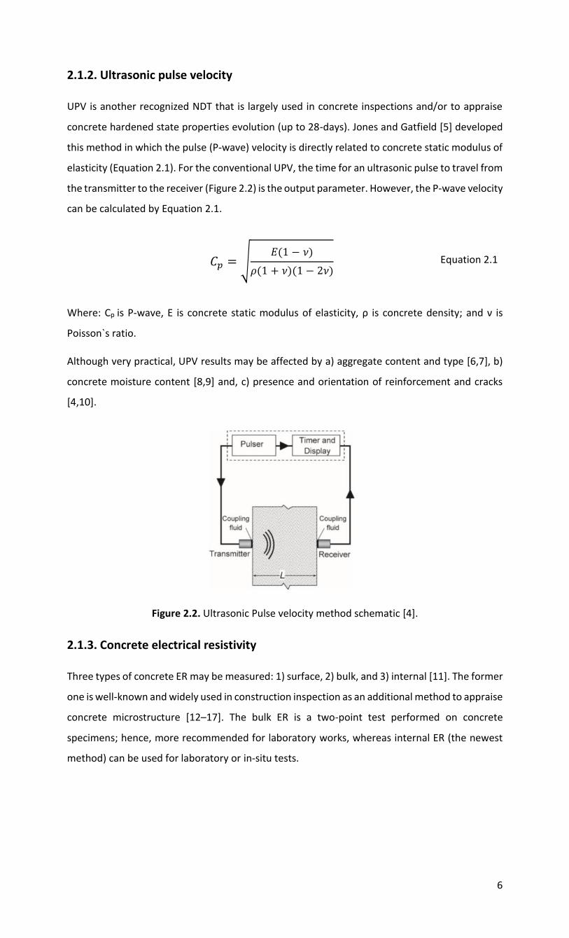
2.1.2. Ultrasonic pulse velocity

UPV is another recognized NDT that is largely used in concrete inspections and/or to appraise

concrete hardened state properties evolution (up to 28-days). Jones and Gatfield [5] developed

this method in which the pulse (P-wave) velocity is directly related to concrete static modulus of

elasticity (Equation 2.1). For the conventional UPV, the time for an ultrasonic pulse to travel from

the transmitter to the receiver (Figure 2.2) is the output parameter. However, the P-wave velocity

can be calculated by Equation 2.1.

𝐶𝑝 = √𝐸(1 − 𝜈)

𝜌(1 + 𝜈)(1 − 2𝜈) Equation 2.1

Where: Cp is P-wave, E is concrete static modulus of elasticity, ρ is concrete density; and ν is

Poisson`s ratio.

Although very practical, UPV results may be affected by a) aggregate content and type [6,7], b)

concrete moisture content [8,9] and, c) presence and orientation of reinforcement and cracks

[4,10].

Figure 2.2. Ultrasonic Pulse velocity method schematic [4].

2.1.3. Concrete electrical resistivity

Three types of concrete ER may be measured: 1) surface, 2) bulk, and 3) internal [11]. The former

one is well-known and widely used in construction inspection as an additional method to appraise

concrete microstructure [12–17]. The bulk ER is a two-point test performed on concrete

specimens; hence, more recommended for laboratory works, whereas internal ER (the newest

method) can be used for laboratory or in-situ tests.

7

2.1.3.1. Test Setups

Surface ER

Surface ER was first applied in geology to determine soil stratification in the field [18].

Furthermore, the Wenner surface ER setup using a four-point approach is the oldest ER type and

is standardized as per AASHTO TP95 [19]. Surface ER is measured using four electrodes equally

spaced as shown in Figure 2.3a. It is worth noting that the two exterior probes measure the

alternating current (i), while the inside probes measure the electrical potential (V). Due to its

interesting configuration along with quick and reliable measurements, this setup has been vastly

used in field concrete. Yet, some factors might result in misleading data if not properly accounted

for such as surface conditions/imperfections, type of electrical current applied, environmental

conditions, presence and orientation of reinforcement and cracks, presence of aggregate on the

concrete surface [20].

Bulk ER

Bulk ER is a two point uniaxial standardized test (ASTM C1876 [21]) as shown in Figure2.3b. A

concrete specimen is placed between the two electrodes with moist sponges, where alternating

current is applied and the drop in the potential between is then measured. Although the test

outcome is the concrete resistance, the bulk ER may be calculated by multiplying the resistance

by the geometrical k-factor (i.e. specimen’s diameter divided by its length). The bulk ER is usually

limited to laboratory applications since the electrode’s assess to concrete members at both sides

is often not possible. Furthermore, the specimen saturation degree is extremely relevant to

perform an accurate measurement through this setup [22].

Internal ER

Internal ER contains two stainless steel probes which are inserted inside the concrete while the

casting process (Figure 2.3c). The internal ER is the only setup able to take measurements in the

fresh and hardened states; moreover, it can be used in the laboratory or in the field in real time

due to the use of wireless sensors. The internal ER is measured between the embedded steel

probes; a geometrical k-factor is determined from the ratio between the resistivity of a known

solution (i.e. NaCl) and the resistance measured by the sensors. Similarly to the bulk ER, the

internal ER is calculated by multiplying the resistance data by the geometrical k-factor. A wide

range of factors may influence on the internal ER outcomes such as presence of reinforcement,

concrete mix-proportioning, and difference in assessment frequency. Thus, is recommended

maintaining the same measurement frequency while the use of the internal ER in the field.

8

a)

b)

c)

Figure 2.3. Electrical resistivity measuring techniques: a) four-point method [23]; b) two-point uniaxial method [24]; c) internal ER sensor setup [25].

2.1.3.2. Overview

ER was first applied in geophysics analysis to quickly assess soils properties in 1912 [26]. However,

only in 1928, Shimizu studied the setting time and ER of cementitious materials [27]. In 1974,

Taylor and Arulanandan [28] studied the electrical conduction of cement hydration products by

varying the frequency (from 1MHz to 100 MHz) of the ER device. This study was divided into two

phases: 1) cement paste mixtures with 0.30 and 0.35 w/c were tested for 1 week to study the

influence of age and w/c on the cement paste’s electrical resistivity and, 2) cement paste

mixtures with three different w/c ratios (i.e. 0.30, 0.35 and 0.40) were assessed up to 24 hours

to better understand the influence of the w/c on weight [28]. These studies outcomes have

proven the efficiency of ER to appraise cement paste mixtures microstructure [28].

In 1975, Spellman and Stratfull [29] developed a research report on how concrete ER could be

used to measure the efficiency of membrane system to prevent corrosion in concrete decks.

Frascoia [30] complemented the former work, testing 32 concrete slabs coated with four

different polyurethane and epoxy coatings. A relationship between chloride penetration and

concrete ER after 730 days of testing was found (Table 2.1). However, only in 1981, [31]

developed a method to determine the concrete chloride permeability, known nowadays as Rapid

Chloride Permeability Test (ASTM C1202 [32]).

9

Table 2.1. Electrical Resistivity measurements to analyze chloride penetration on slabs [30].

Furthermore, in 2003, Chini et al. [33] along with the Florida Department of Transportation

developed an extensive research report involving 132 different concrete mixtures with four

different binders (i.e. Portland cement, fly-ash, ground granulate blast-furnace slag, and silica

fume). This work correlates surface ER with RCPT at 28-day and 91-day. It has been concluded

that a strong relationship between RCPT and surface ER could be experimentally determined,

with R² equal to 0.948 and 0.932 to 28-day and 91-day, respectively as shown in Figure 2.4 [33].

In 2011, Rupnow and Icenogle [34] developed a comparative research report comparing ASTM

C1202 and surface ER at different ages (i.e. 14-day, 28-day, and 56-day) to determine concrete

chloride permeability. Rupnow and Icenogle also established that surface ER could determine

durability parameters and thus it was granted to be a fast, inexpensive alternative to the

conventional RCPT test [34].

a)

b)

Figure 2.4. RCPT and surface ER relationship: a) at 28 days; b) at 91 days [33].

In 2011, surface ER was standardized by the American Association of State Highway and

Transportation Officials - AASTHO TP95 [19]. This standard presents Table 2.2, where the

permeability class of a concrete specimen may be classified through RCPT or surface ER. Besides

10

the good correlation between ER and durability performance, studies [14,35] have proven that

ER could accurately predict compressive strength.

Table 2.2. Relationship between RCPT at 56-day and surface ER at 28 day [19].

2.1.3.3. Impact of external factors on concrete ER

As mentioned before, ER is a reliable and inexpensive NDT that allows fast assessment of

concrete microstructure. Yet, several external parameters (i.e. sample relativity humidity,

temperature, test setup and frequency) affect the ER results.

Saturation degree

One of the well-documented factors that have an influence on ER output is the concrete relativity

humidity (RH). In 2011, Andrade et al. [36] studied the influence of saturation degree on the bulk

ER. Concrete mixtures with two w/c (i.e. 0.40 and 0.70) were mix-proportioned with Portland

cement (type CEM I). It is worth noting that a superplasticizer was added to the former to fix the

same flowability for both mixtures. After curing for 3 and 7 days, samples were prepared, sliced,

and kept at constant temperature (20 ͦC). Moreover, the specimens were placed at different

chambers to control five different RH (i.e. 55%, 65%, 75%, 85%, and 95%). Lastly, Andrade et al.

concluded that concrete ER was exponentially greater with the decrease of specimens’ RH as

shown in Figure 2.5, which might be explained by the change in the pore network connectivity.

Therefore, gauging concrete ER specimen with a low RH might be misleading as it yields greater

concrete ER if compared to the same concrete mixture with greater RH. Therefore, the samples

“pre-conditioning” has been found as an extremely important factor to ensure proper ER

outcomes [36,37]. Hence, ASTM C1760 recommends concrete specimens to be vacuum saturated

prior to testing.

11

Figure 2.5. Relative Humidity effect on concrete ER [36].

Temperature

Another important parameter that influences concrete ER is temperature. In 1995, Elkey and

Sellevold [37] studied the temperature effect of two concrete mixtures under saturated

conditions. The control mixture was developed with 0.6 w/c, whereas the second mixture was

mix-designed with 0.4 w/c and 4.9% replacement of silica fume. The influence of temperature

combined with concrete RH condition was also analyzed. The authors concluded that a change

of 1 Cͦ corresponded to an average ER variation of 3% for the mixes tested, as displayed in Figure

2.6 [37]. However, this variation was also influenced by the specimen’s RH; for instance, a

specimen with 25% RH varied 5% per Cͦ [37]. The decrease in ER due to the temperature rise is

related to the increase in ionic mobility within the concrete pore solution [37]. Therefore, the

specimens should be always at the same temperature to avoid misleading measurements.

Ferreira and Jalalili [35] proved that the effect of temperature can be corrected with an adequate

conversion factor based on Arrhenius equation.

12

Figure 2.6. Temperature effect on concrete ER [37].

Figure 2.7. Sensitivity to temperature influence based on degree of saturation [37].

Signal frequency

Signal frequency is another key factor that influences ER outcomes. In 2015, Layssi et al. [38]

presented a comparison between ER readings varying the signal frequency (i.e. 40 Hz and 1 KHz).

It has been found that a lower frequency signal might increase concrete ER in about 9% when

compared to 1 KHz frequency measurements, as shown in Figure 2.8 [38]. Thus, it is

recommended to apply a signal frequency over 500 Hz, so that ER outcome is not overestimated

[38].

Figure 2.8. Signal frequency influence on concrete ER [38].

13

2.1.3.4. Impact of internal factors on concrete ER

Aggregate

Conventional concrete is normally composed of about 60-70% of aggregates in volume. However,

very limited information is available on the influence of the coarse aggregate type on ER

outcomes. In 1991, Ping et al. [39] performed an experimental study to validate concrete

conductivity models (Figure 2.9) based on the coarse aggregate-paste Interfacial Transaction

Zone (ITZ). The system’s conductivity was calculated through weighted average; i.e., the

summation of each component (i.e., paste, coarse aggregate, and ITZ) conductivity times each

component fraction area [39]. Hence, a new parameter called Interfacial Excess conductance (θ)

was created to appraise ITZ conductivity. Moreover, it has been concluded that the different

types of coarse aggregates (i.e., limestone and glass) do not affect ITZ conductivity. Yet, in 1998,

Tasong et al. [40] analyzed the aggregate and Portland cement GU chemical interactions and

how the aggregate mineralogy would affect the composition (i.e., Ca2+, Mg+, Fe2+,

Al3+,Na+,K+,Si4+,SO42- and OH-) of mortars pore solution. Therefore, four aggregates with different

mineralogy (i.e., basalt, limestone, silica sand, and quartzite) were crushed into fine particles

(1μm to 100μm) and mixed with Portland cement to produce mortar specimens. Pore solution

extraction and Inductively Coupled Plasma Emission Spectrometer (ICP-ES) were performed over

time to understand how the pore solution composition was affected by the aggregate-cement

reaction for each aggregate studied. The authors concluded that the basalt changed significantly

the chemistry of the pore solution (especially the cations) of the mortars while the other

aggregates (i.e., quartzite, silica and limestone) caused minor or no impact on it. Moreover, the

limestone was found to interfere with the hydroxyl ions concentration of the mortars pore

solution. Hence, Tasong and colleagues’ work has proven that the aggregate mineralogy might

influence both the chemistry of the pore solution and the ITZ structure of cementitious materials.

Figure 2.9. Simplified conductivity concrete model proposed by Ping et al.[39].

Moreover, In 1994, McCarter [41] developed and extensive experimental work which appraises

concrete, mortar, and cement paste specimens made of conventional Portland cement and also

a blend of Portland cement and pulverised fuel ash with two replacement levels (10% and 30%).

In this study a uniaxial Electrical Resistivity setup with frequency ranging form 1 Hz to 15 MHz

was used to study the aggregate influence on mixtures ER. Although there are three possible

current percolation paths: a) aggregate and cement-paste in in series; b) aggregate particles in

14

direct contact with other; and c) cement-paste only, as represented in Figure 2.10, case c is the

most likely to happen as aggregate particles present a non-conductive characteristic and are

embedded in an ionically conducting cement-paste matrix.

Figure 2.10. Possible electrical percolation paths [41].

The author concluded that the increase of aggregate volume resulted in an overall growth of the

material’s ER. It may be explained by Figure 2.11 since the increase of the aggregate volume

reduces the cement paste cross-sectional area.

Figure 2.11. Volume of aggregate influence on concrete ER [41].

Similar results were drawn by Shane et al. [42], which appraised the conductivity of mortars made

of Portland Cement (Type I), 0.40 w/c, and sand volume fraction (Vf,sand) ranging from 0.00 to

0.50. Although it is known that ITZ presents lower ER due to higher porosity, the increase of sand

volume displayed a global increase of ER. Therefore, one might conclude that the electrical

blocking effect with the increment of Vf,sand appears to be more significant than the negative

influence of the ITZ on ER [42]. Hence, greater aggregate volume results in lower mortar

conductivity (i.e. higher resistivity) in all hydration periods analyzed, as presented in Figure 2.12.

15

Figure 2.12. Volume of aggregate influence on mortar ER [42].

Princigallo et al. [43] also studied the influence of the aggregates volume on concrete ER. Several

concrete mixtures were developed with 0.37 w/c, Portland cement, and silica fume. The

aggregate volume varied from 0 to 75%. The aggregate volume threshold calculated as 60%

(Figure 2.13) was the main contribution of this study. Similarly to [41,42], the authors confirmed

that the greater the aggregate volume, the greater the concrete ER. Additionally, as shown in

Figure 2.14, it was recommended to account for the aggregate volume when calibration curves

were established to predict the compressive strength through electrical conductivity [43].

Figure 2.13. Concrete normalized electrical conductivity over time varying aggregate volumes

[43].

16

Figure 2.14. Relationship between concrete compressive strength and conductivity for different

aggregate volumes [43].

Similar to NDTs previously presented, the type and maximum size of the coarse aggregate also

affect concrete ER. In 1996, Morris et al. [44] investigated the influence of the type and maximum

size of the aggregate on concrete surface ER. Two coarse aggregate types were selected: 1)

limestone with maximum size of 9.5 mm and 19 mm and, 2) river rock with maximum size of 9.5

mm. As shown in Table 2.3, the maximum aggregate size and nature significantly affected

concrete ER.

Sengul [45] also performed a vast experimental work to evaluate aggregate maximum size and

texture effect on concrete ER. Eight 0.28 w/c Portland cement concrete mixtures were developed

with two types of coarse aggregates (i.e. crushed limestone and rounded siliceous gravel) to

verify its effect on surface ER. Moreover, seven 0.50 w/c concrete mixtures with crushed

limestone were manufactured to analyze the influence of the aggregate’s maximum size (i.e.

4mm and 32mm) on concrete ER. Additionally, four aggregate volumes were selected (i.e. 0%,

20%, 40%, 60% and 73%). Figure 2.15 shows that the higher the aggregate sizes, the greater the

concrete ER for an aggregate content greater than 40% [45]. Moreover, it has been found that

round siliceous gravel aggregates resulted in inferior concrete ER due to its rounded aggregate’s

shape for an aggregate volume higher than 60% (Figure 2.16).

Table 2.3. Influence of aggregate size and type on Electrical Resistivity geometrical factor [44].

17

Figure 2.15. Aggregate size influence on concrete ER [45].

Figure 2.16. Aggregate type influence on concrete ER [45].

An additional concrete parameter that appears to significantly impact on concrete ER is the

aggregate’s mineralogy. For instance, in the field of geophysics, it is well-registered that rocks

with different natures (sedimentary, igneous, and metamorphic) result in different ER, as shown

in Table 2.4. For instance, granite ER ranges from 5 to 5000 kΩ.cm, whereas limestone ER ranges

from 0.05 to 0.4 kΩ.cm. Hence, modern and fast soil surveying techniques rely on the ER

differences of distinct rocks to determine the rock composition on quarry pits [46]. Therefore,

Ping et al. [39] proposed that the overall concrete ER should be determined by the sum of each

individual component ER times its fraction volume.

18

Table 2.4 Rock electrical resistivity by rock lithotype [47]

In 2019, Gulrez and Hartell [46] investigated the influence of coarse aggregate nature on surface

ER. Twenty-one concrete mixtures were manufactured with 0 and 20% replacement of class C

fly-ash mixes, three different types of coarse aggregates (i.e. limestone, dolomite, and gabbro),

and three different w/c (i.e. 0.40, 0.45, and 0.50). It was reported (Figure 2.17) that the

aggregate’s nature had an insignificant-marginal effect on surface ER when analyzing control

mixes (i.e. no fly ash replacement). However, the aggregate nature was considered statically

significant for most w/c when analyzing concrete mixtures containing fly ash class C (Figure 2.18).

The author attributes this concrete ER variation to the difference in the coarse aggregate

properties. However, the authors mentioned that further studies had to be developed in order

to reliably confirm this assumption with different SCMs types and replacement ratios [46].

19

Figure 2.17. Coarse aggregate influence on concrete ER control mixes: a) 0.40 w/c; b) 0.45 w/c;

c) 0.50 w/c [46].

Figure 2.18. Coarse aggregate influence on concrete ER 20% fly ash replacement: a) 0.40 w/c;

b) 0.45 w/c; c) 0.50 w/c [46].

20

In conclusion, the aggregate volume, maximum size, texture, and nature were significant factors

when overall analyzing concrete ER. Yet, very few research and literature can be found regarding

the influence of the aggregate’s nature on concrete ER. Moreover, further studies should be

performed to fully perceive the latter when cementitious materials are manufactured with

distinct types and amount of SCMs.

Binder type and replacement amount

Besides the aggregates’ characteristics and volume, the binder type and replacement amount are

also known as key internal factors that affect concrete ER. SCMs, by-products from distinct

industries (steel, coal, etc.) are used as a replacement of Portland cement to enhance the

material’s eco-efficiency and cost-efficiency. However, the use of SCMs also presents important

microstructure benefits since they usually reduce the material’s overall porosity and

permeability; hence, ensuring better durability properties [48].

In 1994, Tashiro et al. [49] evaluate the possibility of measuring the pozzolanic activity of pastes

through ER. Eight pastes were manufactured with 0.50 and 0.70 w/c incorporating different types

of SCMs, as presented in Table 2.5. Moreover, the authors divided the SCMs into four groups

according to the ER increase over time (Figure 2.19 and Figure 2.20). Category 1 (mixtures with

silica fume, acid clay, and zeolite) resulted in a sharp and quickly rise of ER which becomes

constants after 12 hours. Category 2 (fly ash mixtures) yielded a sharp rise after 24 hours.

Category 3 (kaolin mixtures) presented no sharp rise; yet ER starts gradually increasing after 24

hours. Finally, Category 4 (Quartz mixtures) showed neither sharp increase nor marked increase

of ER [49].

Table 2.5. Paste specifications [49].

21

Figure 2.19. Paste resistivity evolution over-time from paste mixtures 1 to 4 together with 8

[49].

Figure 2.20. Paste resistivity evolution over-time from paste mixtures 5 to 8 [49].

Regarding Portlandite consumption, it was concluded that silica fume, acid clay, and zeolite

mixtures consumed 100% of Portlandite in less than 3 hours. Kaolin also presented a fast

decrease in Portlandite due to its high reactivity (i.e. approximately 70% of Portlandite

consumption). Fly ash also presented a high-decrease of Portlandite; however, the only 20-30%

of Portlandite was consumed and it was retarded due to fly ash initial stage of hydration [49], as

shown in Figure 2.21. Hence, Tashiro concluded that ER was a reliable technique able to rapidly

evaluate SCMs pozzolanic activity on pastes [49].

Figure 2.21. Portlandite consumption for 10% dosage [49].

22

McCarter et al. [50] also investigated the influence of SCMs on mortars. A total of five mixtures

(Table 2.6) were elaborated containing pure Portland cement (PC) and a combination of PC with

others SCMs (i.e. ground granulated blast-furnace slag - GGBS, metakaolin - MK, and micro-silica

- MS). Figure 2.22 shows a decrease of conductivity (i.e. increase in ER) for all the mixes using

SCMs when comparing to control mixtures. According to the authors, this increment on mortar

ER is related to two possible factors: a) pozzolanic materials usually results in a finer and more

tortuous pore network than PC and b) change in pore-solution ionic concentration due to a

change in mineralogical phases solubility [50]. The study also compared the evolution of pore-

solution conductivity and mortar electrical conductivity concluding that mortar conductivity

increases at a faster pace when compared to pore-solution conductivity [50]. Therefore, the

improvement on mortar microstructure (and thus higher ER) has a higher likelihood to be related

to an improvement in pore tortuosity and pore construction rather than mortar pore-solution ER

increase [50].

Table 2.6. Mortar mix-proportions [50].

Figure 2.22. Conductivity evolution over-time [50].

[51] studied the influence of three different SCMs and PC replacement (i.e. 35% GGBS, 20% fly

ash Class C, and 7% silica fume) on concrete ER. It was observed that control mixes presented

lower conductivity (i.e. higher ER) at early ages when compared to SCMs mixtures, except the

silica fume mix that presented higher ER after 2 days (Figure 2.23). However, GGBS and fly ash

mixtures overcame control mixtures ER at approximately 7 days [51]. Those results are in

accordance with past literature [49,50], as pozzolans are well-documented to consume concrete

Portlandite formed from convention Portland cement hydration to produce new hydration

23

products (C-S-Hp). Hence, the system porosity decreases, improving concrete microstructure and

concrete ER [51–53]. Furthermore, according to [54], the addition of fly ash on concrete mixtures

also improves concrete packing density, reducing in that way, the system porosity due to its

reduced particle size distribution (i.e. filler effect).

Figure 2.23. Conductivity evolution over-time for 0.40 w/c samples [51].

One of the reasons that SCMs increases concrete ER is the increase of concrete pore-solution

resistivity as it was previously suggested by [50]. In 2015, Sallehi [55] developed a research

project to analyze the influence of the binder type (i.e. 10% silica fume, 30% fly ash, 30% GGBS)

on 0.45 w/c ratio pastes on the fresh pore-solution resistivity. It is worth noting that two PC

pastes were developed (control mixtures and a mixture containing 0.50% superplasticizer based

on the cement mass). ER was measured in three different extraction times (30, 60, and 90

minutes). It was observed a constant decrease in pore-solution ER for the first 2 hours after

mixing for all mixtures. According to the authors, this decrease is attributed to the concentration

of ions in the pore-solution due to chemical reactions at the first 2 hours after mixing [55]. It was

also observed that all studied pastes and pore-solutions containing SCMs or superplasticizer

presented greater ER when compared to the control mixt with no superplasticizer (P0.45), as

presented in Table 2.7.

Table 2.7. Fresh pore solution and pastes ER [55].

24

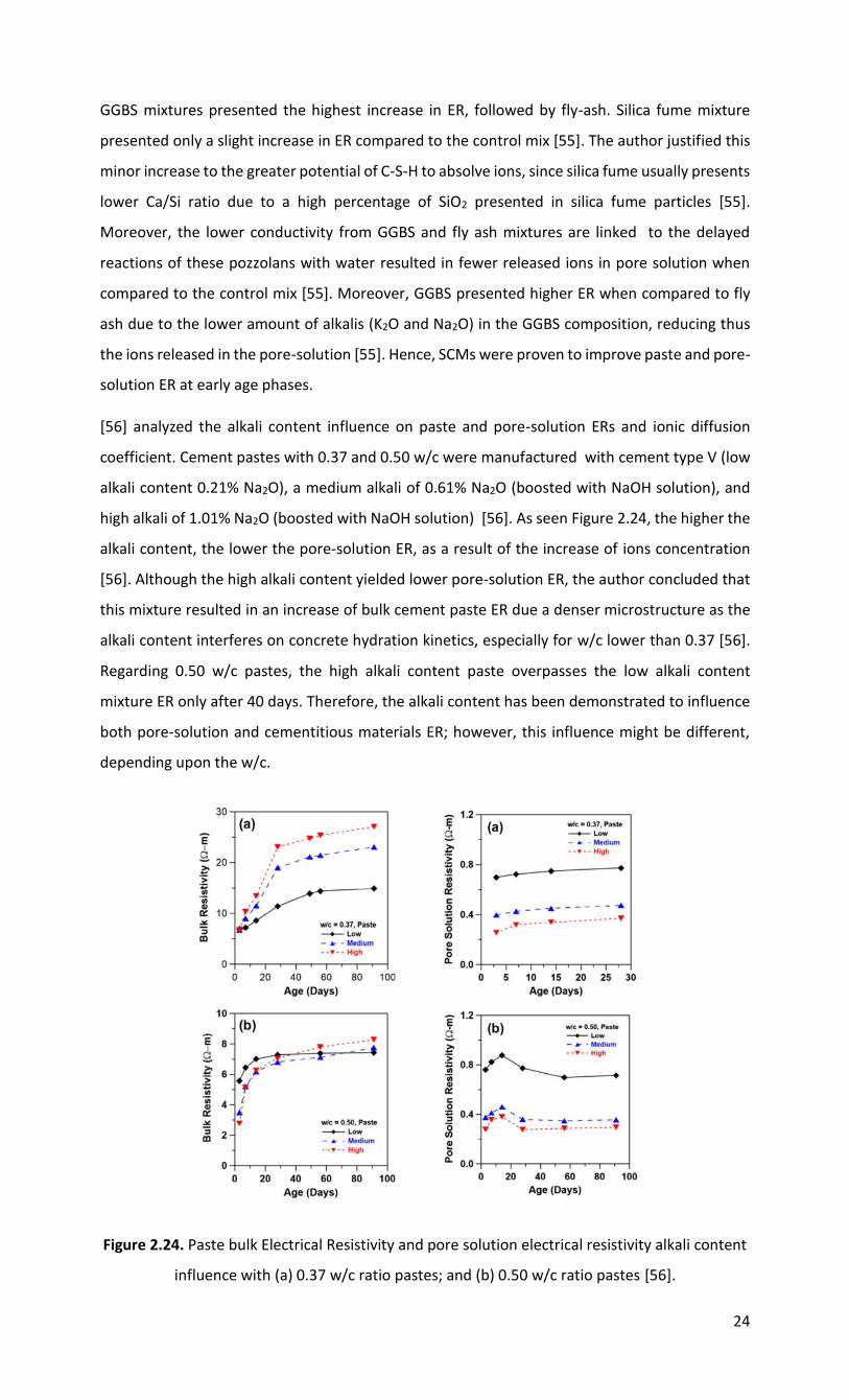
GGBS mixtures presented the highest increase in ER, followed by fly-ash. Silica fume mixture

presented only a slight increase in ER compared to the control mix [55]. The author justified this

minor increase to the greater potential of C-S-H to absolve ions, since silica fume usually presents

lower Ca/Si ratio due to a high percentage of SiO2 presented in silica fume particles [55].

Moreover, the lower conductivity from GGBS and fly ash mixtures are linked to the delayed

reactions of these pozzolans with water resulted in fewer released ions in pore solution when

compared to the control mix [55]. Moreover, GGBS presented higher ER when compared to fly

ash due to the lower amount of alkalis (K2O and Na2O) in the GGBS composition, reducing thus

the ions released in the pore-solution [55]. Hence, SCMs were proven to improve paste and pore-

solution ER at early age phases.

[56] analyzed the alkali content influence on paste and pore-solution ERs and ionic diffusion

coefficient. Cement pastes with 0.37 and 0.50 w/c were manufactured with cement type V (low

alkali content 0.21% Na2O), a medium alkali of 0.61% Na2O (boosted with NaOH solution), and

high alkali of 1.01% Na2O (boosted with NaOH solution) [56]. As seen Figure 2.24, the higher the

alkali content, the lower the pore-solution ER, as a result of the increase of ions concentration

[56]. Although the high alkali content yielded lower pore-solution ER, the author concluded that

this mixture resulted in an increase of bulk cement paste ER due a denser microstructure as the

alkali content interferes on concrete hydration kinetics, especially for w/c lower than 0.37 [56].

Regarding 0.50 w/c pastes, the high alkali content paste overpasses the low alkali content

mixture ER only after 40 days. Therefore, the alkali content has been demonstrated to influence

both pore-solution and cementitious materials ER; however, this influence might be different,

depending upon the w/c.

Figure 2.24. Paste bulk Electrical Resistivity and pore solution electrical resistivity alkali content

influence with (a) 0.37 w/c ratio pastes; and (b) 0.50 w/c ratio pastes [56].

25

2.1.4. Determination of compressive strength through ER.

Although concrete ER has been studied for nearly a century [27], only in 2006, Wei and Li [12]

were able to reliably measure the setting time and w/c of paste mixtures with three different w/c

(i.e. 0.30, 0.35, and 0.40) both in the fresh and hardened states (i.e. 8h, 12h, and 24h), as per

Figure 2.26. Finally, it was concluded that ER presented an inverse relationship with the paste’s

w/c for all ages tested (e.g. the higher the w/c, the lower the resistivity). The setting time was

also affected by the w/c, that is, with the increase of w/c the initial setting was delayed [12].

Figure 2.25. Non-contact Electrical Resistivity meter device schematic [13].

Figure 2.26. Concrete w/c ratio versus Electrical Resistivity for different ages [12].

In 2010, Mancio et al. [14] developed a new concrete ER meter (Figure 2.27), based on a well-

documented electrode array usually applied in geophysics studies (Wenner-probe array). The

probe consists of four stainless-steel electrodes equally separated at a distance of 2.5 cm by an

electrical isolator plastic body and can be submerged in fresh concrete. The two outer electrodes

are submitted to a high frequency (1000 Hz) and an AC current with 1.5V; subsequently,

voltmeters connected to a known resistor and inner electrodes in parallel displays the voltage

drop among the elements (Vo and Vc). The current (Io) can be calculated dividing Vo by the

electrical resistance (Ro). Moreover, concrete electrical resistance (Rc) is determined dividing Vc

by Io. Finally, to determine concrete ER a geometrical factor (k) has to be multiplied by Rc [14].

Eight different concrete mixtures were developed with distinct w/c (i.e. 0.3, 0.4, 0.5, and 0.6) and

different binders (i.e. 100% PC and 25% Class F fly-ash replacement) [14].

.

26

Figure 2.27. Submerged Electrical Resistivity meter [14].

It was concluded that ER was able to reliably measure the concrete w/c with a low coefficient of

variance (2.10% - 6.41%) for both control and fly-ash concrete mixtures as shown in Figure 2.28.

Therefore, one may conclude that an accurate prediction of compressive strength can also be

made through ER since concrete compressive strength is mainly affected by w/c.

a)

b)

Figure 2.28. Relationship between w/c and concrete ER: a) control concrete samples; b) class-F

fly-ash mixtures [14].

In 2009, Ferreira and Jalali [35] used an ER Wenner probe setup (surface ER) to predict concrete

compressive strength at 28 days using 7-day and 28-day surface ER measurements. Concrete

mixtures were mix-designed with two different w/c (i.e. 0.4 with cement type I and 0.5 with

cement type IV) [35]. Ferreira and Jalali analyzed two different approaches to estimate concrete

compressive strength: 1) empirical approach, which is based on calibration curves and, 2) a

theoretical approach founded in Avrami work [57]. In this work, an ER correction is performed by

determining a relationship between any given temperature and 20 Cͦ concrete ER, based on

Arrhenius equation [35]. It was concluded that the theoretical approach (based on 7-day ER)

yielded inferior error on 0.4 w/c (11%) than 0.5 w/c (23%) mixtures. Furthermore, when using

28-day ER data (Figure 2.29) in both approaches, the error decreased (i.e. 4% and 9% for the

empirical and theoretical method, respectively). Moreover, it has been proven that the

27

temperature effect on ER outputs could be corrected by an adequate conversion factor based

on Arrhenius equation [35].

a)

b)

Figure 2.29. Compressive strength and concrete ER relationship: a) 0.5 w/c mixtures; b) 0.4 w/c

mixtures [35].

In summary, ER has proven to be one of the most powerful NDTs able to predict concrete w/c,

and compressive strength development over-time in an inexpensive, fast, and reliable fashion.

Yet, as it has been demonstrated over this section, the concrete raw materials (i.e. binder type

and replacement level) [14,35], aggregate volume [4,6,8], and aggregate type [4,6,8]) may result

in misleading correlation with concrete microstructure whether they are not properly accounted

for when the measurements are performed.

2.2. Science gap

Although ER is found in the literature as a reliable NDT technique that can be used to appraise

concrete microstructure and predict compressive strength, it may be affected by a wide number

of external (i.e. saturation degree, temperature, test setup and frequency) and internal (i.e.

aggregate and SCMs type and/or amount) factors. Yet, a deeper and quantitative understanding

of the influence of the aggregate lithotype (i.e. mineralogy) along with the SCMs type and amount

on ER outcomes is imperative to reliably use this technique for practical purposes. The latter is

especially important while the use of distinct ER setups, which normally yield distinct outcomes.

Thus, this project aims thoroughly assess the influence of the coarse aggregate nature and binder

type/amount on concrete ER. Moreover, the prediction of concrete compressive strength

through ER data is performed to evaluate the reliability of the method when the raw material’s

differences are accounted for.

28

2.3. References

[1] W. Martínez-Molina et al., “Predicting Concrete Compressive Strength and Modulus of

Rupture Using Different NDT Techniques,” Adv. Mater. Sci. Eng., pp. 1–15, Oct. 2014, doi:

10.1155/2014/742129.

[2] R. Pucinotti, “Reinforced concrete structure : Non destructive in situ strength assessment

of concrete,” Constr. Build. Mater., vol. 75, pp. 331–341, 2015, doi:

10.1016/j.conbuildmat.2014.11.023.



10.1155/2014/742129.


Mater. J., no. January, pp. 1–52, 2019.

[5] R. Jones, “The non-destructive testing of concrete,” vol. 40, no. 1940, pp. 1113–1121,

1945.

[6] J. A. Bogas, M. G. Gomes, and A. Gomes, “Compressive strength evaluation of structural

lightweight concrete by non-destructive ultrasonic pulse velocity method,” Ultrasonics,

vol. 53, no. 5, pp. 962–972, 2013, doi: 10.1016/j.ultras.2012.12.012.

[7] B. S. Al-Nu’man, B. R. Aziz, S. A. Abdulla, and S. E. Khaleel, “Effect of Aggregate Content

on the Concrete Compressive Strength - Ultrasonic Pulse Velocity Relationship,” Am. J.

Civ. Eng. Archit., vol. 4, no. 1, pp. 1–5, 2017, doi: 10.12691/ajcea-4-1-1.


[9] J. P. GODINHO, T. F. DE SOUZA JÚNIOR, M. H. F. MEDEIROS, and M. S. A. SILVA, “Factors

influencing ultrasonic pulse velocity in concrete,” Rev. IBRACON Estruturas e Mater., vol.

13, no. 2, pp. 222–247, 2020, doi: 10.1590/s1983-41952020000200004.

[10] N. Fodil, M. Chemrouk, and A. Ammar, “The influence of steel reinforcement on

ultrasonic pulse velocity measurements in concrete of different strength ranges,” IOP

Conf. Ser. Mater. Sci. Eng., vol. 603, no. 2, 2019, doi: 10.1088/1757-899X/603/2/022049.


electrical resistivity measurements in cementitious systems,” Transp. Res. Rec., vol. 000,

no. 2342, pp. 90–98, 2013, doi: 10.3141/2342-11.



10.1061/(ASCE)0899-1561(2006)18:1(99).

[13] Z. Li, X. Wei, and W. Li, “Preliminary Interpretation of Portland Cement Hydration Process

29

Using Resistivity Measurements,” ACI Mater. J., vol. 100, no. 3, Feb. 2003, doi:

10.14359/12627.


Situ Determination of Water-Cement Ratio of Fresh Concrete,” ACI Mater. J., vol. 107, no.

6, Oct. 2010, doi: 10.14359/51664045.

[15] R. B. Polder, “Test methods for on site measurement of resistivity of concrete a RILEM

TC-154 technical recommendation,” p. 7, 2001.



10.1016/j.conbuildmat.2011.12.111.


determine initial setting time of cement and concrete using plate test,” Mater. Struct.,

vol. 49, no. 8, pp. 3135–3142, Oct. 2016, doi: 10.1617/s11527-015-0709-0.

[18] AASHTO, “Standard test method for surface resistivity of concrete`s ability to resist

chloride ion penetration.,” AASTHO TP95, vol. Washigton, p. DC: AASHTO., 2014.

[19] ASTM C1876, “Standard Test Method for Bulk Electrical Conductivity of Hardened

Concrete,” pp. 1–5, 2012, doi: 10.1520/C1876-19.

[20] “Surf | Concrete Surface Resistivity | Giatec Scientific Inc.” [Online]. Available:

https://www.giatecscientific.com/products/concrete-ndt-devices/surf-surface-

resistivity/. [Accessed: 19-Jun-2020].

[21] “RCON | Concrete Bulk Resistivity | Giatec Scientific Inc.” [Online]. Available:

https://www.giatecscientific.com/products/concrete-ndt-devices/rcon-bulk-resistivity/.

[Accessed: 19-Jun-2020].

[22] Giatec, “SmartBox,” 2020. [Online]. Available:

https://www.giatecscientific.com/products/concrete-sensors/smartbox-electrical-

resistivity/. [Accessed: 15-Mar-2020].

[23] A. Samouëlian, I. Cousin, A. Tabbagh, A. Bruand, and G. Richard, “Electrical resistivity

survey in soil science: A review,” Soil Tillage Res., vol. 83, no. 2, pp. 173–193, 2005, doi:

10.1016/j.still.2004.10.004.

[24] Y. Shimizu, “An electrical method for measuring the setting time of portland cement,”

Mill Sect. Concr., vol. 32, no. 5, pp. 111–113, 1928.

[25] M. A. Taylor and K. Arulanandan, “RELATIONSHIPS BETWEEN ELECTRICAL AND PHYSICAL

PROPERTIESOF CEMENTPASTES,” vol. 4, pp. 881–897, 1974.

[26] D. L. Spellman and R. F. Stratfull, “EVALUATION OF BRIDGE DECK MEMBRANE SYSTEMS

30

AND MEMBRANE EVALUATION PROCEDURES,” 1975.

[27] R. I. Frascoia, “Vermont’S Experience With Bridge Deck Protective Systems.,” ASTM Spec.

Tech. Publ., no. 629, pp. 69–81, 1977, doi: 10.1520/stp27954s.

[28] D. Whiting, “Report No. FHWA/RD-81/119 Rapid Determination of the Chloride

Permeability of Concrete Final,” Washington, 1981.

[29] ASTM C1202, “Standard Test Method for Electrical Indication of Concrete’s Ability to

Resist Chloride Ion Penetration,” Am. Soc. Test. Mater., no. C, pp. 1–8, 2012, doi:

10.1520/C1202-12.2.

[30] A. R. Chini, L. C. Muszynski, and J. Hicks, “Determination of Acceptance Permeability

Characteristics for Performance-Related Specifications for Portland Cement Concrete,”

no. July, pp. 1–165, 2003.

[31] T. D. Rupnow and P. Icenogle, “Evaluation of Surface Resistivity Measurements as an

Alternative to the Rapid Chloride Permeability Test for Quality Assurance and Acceptance

July 2011 LTRC Project Number : 10-1C SIO Number : 30000111 Louisiana Transportation

Research Center 4101 Gourrie,” 2011.

[32] R. M. Ferreira and S. Jalali, “NDT measurements for the prediction of 28-day compressive

strength,” NDT E Int., vol. 43, no. 2, pp. 55–61, 2009, doi: 10.1016/j.ndteint.2009.09.003.



10.1002/maco.201005777.

[34] W. Elkey and E. J. Sellevold, “Electrical resistivity of concrete,” Nor. Road Res. Lab., p. 33,

1995.

[35] H. Layssi, P. Ghods, A. R. Alizadeh, and M. Salehi, “Electrical Resistivity of Concrete,” p. 6.

[36] X. Ping, J. J. Beaudoin, and R. Brousseau, “Flat aggregate-portland cement paste

interfaces, I. Electrical conductivity models,” Cem. Concr. Res., vol. 21, no. 4, pp. 515–

522, Nov. 1991, doi: 10.1016/0008-8846(91)90101-M.

[37] W. J. Mccarter, “A PARAMETRIC STUDY OF THE IMPEDANCE CHARACTERISTICS OF

CEMENT-AGGREGATE SYSTEMS DURING EARLY HYDRATION,” vol. 24, no. 6, pp. 1097–

1110, 1994.

[38] J. D. Shane, T. O. Mason, and H. M. Jennings, “Effect of the Interfacial Transition Zone on

the Conductivity of Portland Cement Mortars,” ACI Struct. J., vol. 83, no. 5, pp. 1137–

1144, 2000, doi: 10.14359/7403.

[39] A. Princigallo, K. van Breugel, and G. Levita, “Influence of the aggregate on the electrical

conductivity of Portland cement concretes,” Cem. Concr. Res., vol. 33, no. 11, pp. 1755–

31

1763, Sep. 2003, doi: 10.1016/S0008-8846(03)00166-2.

[40] W. Morris, E. I. Moreno, and A. A. Sagues, “PRACTICAL EVALUATION OF RESISTIVITY OF

CONCRETE IN TEST CYLINDERS USING A WENNER ARRAY PROBE,” Cem. Concr. Res., vol.

26, no. 12, pp. 1779–1787, 1996, doi: https://doi.org/10.1016/S0008-8846(96)00175-5.

[41] O. Sengul, “Use of electrical resistivity as an indicator for durability,” Constr. Build.

Mater., vol. 73, pp. 434–441, 2014, doi: 10.1016/j.conbuildmat.2014.09.077.



5533.0002661.

[43] M. A. M. Fadel, H. Zabidi, and K. S. Ariffin, “Monitoring the Quarry Pit Development,”

Procedia Chem., vol. 19, pp. 721–728, 2016, doi: 10.1016/j.proche.2016.03.076.

[44] P. K. Metha and P. J.M. Monteiro, Concrete Miscrostructure, Properties and Mateirals,

3rd ed. McGraw Hill, 2006.

[45] C. Tashiro, K. Ikeda, and Y. Inoue, “EVALUATION OF POZZOLANIC ACTIVITY BY THE

ELECTRIC RESISTANCE MEASUREMENT METHOD,” Cem. Concr. Res., vol. 24, no. 6, pp.

1133–1139, 1994.

[46] W. J. McCarter, G. Starrs, and T. M. Chrisp, “Electrical conductivity, diffusion, and

permeability of Portland cement-based mortars,” Cem. Concr. Res., vol. 30, no. 9, pp.

1395–1400, 2000, doi: 10.1016/S0008-8846(00)00281-7.

[47] M. Nokken, A. Boddy, X. Wu, and R. D. Hooton, “Effects of temperature, chemical, and

mineral admixtures on the electrical conductivity of concrete,” J. ASTM Int., vol. 5, no. 5,

pp. 1–9, 2008, doi: 10.1520/JAI101296.

[48] J. Hill and J. H. Sharp, “The mineralogy and microstructure of three composite cements

with high replacement levels,” Cem. Concr. Compos., vol. 24, no. 2, pp. 191–199, Sep.

2002, doi: 10.1016/S0958-9465(01)00041-5.

[49] P. Ghosh and Q. Tran, “Correlation Between Bulk and Surface Resistivity of Concrete,”

Int. J. Concr. Struct. Mater., vol. 9, no. 1, pp. 119–132, 2015, doi: 10.1007/s40069-014-

0094-z.

[50] K. H. Khayat, “Influence of Supplementary Cementitious Materials and Fillers on

Rheological Properties, Kinetics of Cement Hydration, and Compressive Strength of

Concrete-Equivalent Mortar of SCC... High-Volume Recycled Materials for Sustainable

Pavement Construction Vi,” 2010, pp. 381–392.

[51] H. Sallehi, “Characterization of Cement Paste in Fresh State Using Electrical Resistivity

Technique Affairs in partial fulfillment of the requirements for the degree of Master of

Applied Science,” 2015.

32

[52] Y. Bu and J. Weiss, “The influence of alkali content on the electrical resistivity and

transport properties of cementitious materials,” Cem. Concr. Compos., vol. 51, pp. 49–

58, 2014, doi: 10.1016/j.cemconcomp.2014.02.008.

[53] M. Avrami, “Granulation, phase change, and microstructure kinetics of phase change.

III,” J. Chem. Phys., vol. 9, no. 2, pp. 177–184, Feb. 1941, doi: 10.1063/1.1750872.

33

3. Chapter Three: The Influence of the Binder Type & Aggregate Nature on the Electrical Resistivity of Conventional Concrete

Hugo Deda¹, Leandro Sanchez¹

¹Department of Civil Engineering, University of Ottawa, CANADA

Abstract

Early-age mechanical properties are becoming more critical nowadays to optimize construction

scheduling. Several advanced techniques have been proposed in this regard and among those,

electrical resistivity (ER) has been showing promising results. Yet, recent literature data have

evidenced that ER might be significantly influenced by a variety of parameters such as the

supplementary cementing materials (SCM) type/amount and aggregates nature used in the mix.

These factors can hinder the practical benchmark of concrete mixtures proportioned with distinct

raw materials. This work aims to appraise the influence of the coarse aggregate nature and binder

replacement/amount on concrete ER and compressive strength prediction models through ER

measurements using 24 mixtures manufactured with two different coarse aggregates natures

(i.e. granite and limestone), two water-to-binder ratios (i.e. 0.6 and 0.4), and incorporating two

different SCMs (i.e. slag, and fly-ash class F) with different replacement levels. Three distinct ER

techniques (e.g. bulk, surface, and internal) and compressive strength tests were performed at

different concrete ages (i.e. 3, 7, 14, and 28 days). Results indicated that the binder type and

replacement amount significantly affect ER and compressive strength. The coarse aggregate

nature presented minor influence for “ordinary” quality mixtures, while showing important

impact on refined microstructure mixes. Finally, ER techniques, especially internal ER, were found

to be quite reliable to predict the compressive strength of conventional concrete made of single,

binary and ternary binder blends.

Keywords: Electrical resistivity, non-destructive testing, concrete microstructure,

supplementary cementitious materials.

34

3.1. Introduction

Concrete is the most consumed construction material worldwide due to its interesting fresh,

hardened, and durability-related properties [1]. Although all these advantages, the construction

industry is currently facing distinct types of challenges and amongst those, construction

scheduling has become quite crucial. In this context, the compressive strength of concrete (i.e.

28-day value) is one of the most important properties of the material and is often used as a

quality control indicator. Usually, concrete specimens are manufactured and tested over time

(i.e. 3, 7, 14 and 28 days) to appraise their strength development and thus evaluate the possibility

of a timely removal of formworks [2,3]. The faster the formworks removal, the more optimized

(i.e. lower cost) the construction scheduling [2,3]. However, testing concrete specimens is time

consuming and generates a huge amount of waste that might be avoided. Therefore, several

advanced non-destructive techniques (NDT; e.g. rebound hammer [4], ultrasonic pulse velocity

[5], microwave techniques [6,7], electrical resistivity (ER) [8–10] etc.) have been proposed to

replace the conventional compressive strength test as a quality control indicator of the material.

Yet, the first three aforementioned NDT methods rely on indirect relationships between concrete

properties and compressive strength, which may introduce important variability in the outcomes.

Moreover, concrete raw materials and specimen parameters/conditions might bring uncertainty

to those methods if not properly accounted for such as: a) aggregate type and content [11], b)

moisture content [12], c) curing process [4] and, d) presence and orientation of cracks or

reinforcement [4]. Furthermore, microwave methods are usually performed to determine the

water-to-cement ratio (w/c) of the mixture; however, they do not intend to directly estimate

compressive strength since some other parameters may also influence on strength gain over time

such as curing period and procedure [13], curing temperature [14], SCM type, replacement

amount, etc. Another important disadvantage of this method is the safety concern regarding the

test of aggregates bearing metals in the microwave [7].

In this context, it has been found that ER, a non-destructive and inexpensive technique, is one of

the most suitable NDT methods available to characterize concrete microstructure, and thus

evaluate mechanical and durability-related properties of cementitious materials over time [8–

10]. Although ER is a promising technique used worldwide, recent studies show that it may be

significantly influenced by a wide range of parameters such as a) test setup (i.e. surface ER vs

bulk ER vs internal ER)[15]; b) material’s porosity [16] and moisture content [17]; c) binder

type/amount (e.g. Portland cement, fly ash and slag), and; d) the nature of the aggregates used

in the mix (e.g. lithotype) [18]. However, although the above parameters are known to influence

on ER results, there is still a lack of quantitative data in the literature showing how much ER

results are impacted by the above parameters, especially for mixtures incorporating distinct

binder types, amounts and aggregate natures.

35

3.2. Background

Compressive strength, typically measured over time yet especially at 28 days, is one of the most

important concrete parameters and is often used as an indicator of its “microstructure quality”.

Otherwise, pressure is intensifying in the market to speed up construction scheduling and thus

diminish construction timelines which makes imperative to have a fast, thorough, and reliable

control of the “early-age” mechanical properties of concrete. In this context, It has been reported

that concrete ER could be implemented in field activities to determine or estimate important

concrete parameters such as: a) compressive strength [19–22], b) chloride diffusion coefficient

and corrosion rate [23], and c) initial setting time [24], etc. Nonetheless, there is currently a wide

range of ER devices (i.e. surface, bulk, and internal) in the market, which display distinct concepts

and thus may yield quite different outcomes. Furthermore, the standardization of distinct ER

setups has been quite slow, which prevents a quantitative correlation amongst setups and a deep

understanding on the main parameters influencing each of them. Nowadays, only surface ER

(AASHTO TP95) [25] and bulk ER (ASTM C1760) [26] have already been adopted as a standard

test protocols.

3.2.1. Influence of external factors on concrete ER

Saturation degree

Concrete moisture (i.e. relativity humidity - RH) or degree of saturation is one of the main

external factors that influence ER appraisements. Andrade et al. [17] studied the influence of the

saturation degree on the bulk ER of two concrete mixtures made of Portland cement type CEM I

and displaying two w/c (i.e. 0.40 and 0.70). Moreover, the evaluated specimens were kept at a

constant temperature (i.e. 20 ͦC) and presenting distinct moisture contents (i.e. 55%, 65%, 75%,

85%, and 95% R.H.). It was concluded that ER was much higher with the decrease of the

specimen’s RH due to the change in the pore solution resistivity [19]. The specimen with 65% RH

yielded approximately 10 times greater ER results than the mixture with 95% RH at 18 days.

Therefore, the samples “pre-conditioning” has been found as an extremely important factor to

ensure proper ER outcomes [17,27]. Hence, ASTM C1760 recommends concrete specimens to be

vacuum saturated prior to testing.

Temperature

Another important parameter that influences ER outcomes in concrete is temperature. Elkey and

Sellevold [27] studied the temperature effect on two concrete mixtures under saturated

conditions where the control mixture displayed a w/c of 0.6 and the other mix presented a w/c

of 0.4 and 4.9% replacement of Portland cement (PC) by silica fume). The authors concluded that

a change of 1 ͦC corresponded to an average ER variation of 3% for the mixes tested. However,

this variation was also influenced by the specimen’s RH; for instance, a specimen with 25% RH

varied 5% per ͦC [27]. The decrease in ER due to temperature rise is related to the increase in

36

ionic mobility within the concrete pore solution [27]. Therefore, the specimens should be always

at the same (or at least very close) temperature to avoid misleading measurements. The latter

may pose some important practical challenges to ER appraisements since temperature cannot

be controlled in the field; thus, ER outcomes would require correction prior to be interpreted and

or compared to known/standard values.

Signal frequency

Signal frequency is another important factor that influences ER outcomes. Layssi et al. [28]

presented a comparison between ER readings varying the signal frequency (i.e. 40 Hz and 1 KHz).

It has been found that a lower frequency signal might increase concrete ER in about 9% when

compared to 1 KHz frequency measurements [28]. Thus, it is recommended to apply a signal

frequency over 500 Hz, so that ER outcome is not overestimated [28].

Test setup

ER tests setup is also an important factor to have in mind when analyzing the test outcomes.

Varying ER setups (i.e. surface ER, bulk ER, and internal ER) implicates on modifying resistivity

geometric k-factor [15]. However, besides K-factor, ER is also influenced by a number of other

external parameters aforementioned; hence, a scale factor should be determined to correct and

thus enable correlation amongst distinct ER setups.

3.2.2. Influence of internal factors on concrete ER

Aggregate

Although aggregates generally account for 60-70% of the concrete total volume, limited

information is available on the influence of the coarse aggregate type on ER outcomes. It is known

that coarse aggregates (CA) present significantly higher resistivity (i.e. 104 – 108 Ω.cm) when

compared to cement pastes (i.e. 100 Ω.cm) [29]. Thereby, from the ER point of view, concrete

may be analyzed as a gathering of non-conductive aggregate particles surrounded by an ionically

conductive cement paste matrix [29]. It is well recognized that different mineralogy effects the

rocks properties such as resistivity. Fadel evidenced that igneous rocks present higher ER when

compared to sedimentary rocks; for instance, granite ER ranges from 5000 to 5x106 kΩ.cm,

whereas limestone ER ranges from 50 to 4x10² kΩ.cm [30]. This represents an increase that might

range from 100 to 12500 on the aggregate’s ER. Yet, the aggregate’s influence on the concrete

ER has barely been studied. Moreover, it has been found that ER is quite influenced by the volume

fraction of aggregates in concrete [29,31,32]. An increase in the aggregate volume from 10% to

75% would increase ER outcomes by 500% [29].

The coarse aggregate shape and texture may also impact on concrete ER, since they directly

interfere on the paste-aggregates bonding quality (the so-called interfacial transition zone - ITZ)

and tortuosity [32]. For instance, comparing two concrete mixtures with 80% of aggregates in

volume, the mixture made of crushed limestone results in approximately 63% higher ER than the

37

concrete made of gravel [32]. Yet, very little research has been performed on the impact of the

aggregates nature (i.e. lithotype) and features on ER results [18,33]. Finally, Gulrez and Hartell

have proven a marginal to insignificant difference when comparing three distinct types of coarse

aggregate (i.e. limestone, dolomite, and gabbro) with ordinary Portland cement (PC) concrete.

However, the same aggregates were observed to significantly change ER outcomes in concrete

mixtures incorporating 20% of fly-ash type C [18].

Binder type and replacement amount

Besides the aggregate nature, the type of binder is acknowledged to play an important role on

the concrete ER. SCMs are normally used as a partial replacement of PC to improve the fresh and

hardened state properties of concrete, while improving its sustainability and cost due to PC

reduction [34]. SCMs are known to have a major impact on concrete microstructure (and thus on

ER appraisal). Lataste et al. [35] compared the differences of ER data gathered on concrete

mixtures presenting distinct types of binders (i.e. PC, fly ash, and silica fume). According to the

authors, ER results might be increased by ten times while the use of SCMs in concrete such as

silica fume [35]. The latter has been explained by the formation of new hydration products (C-S-

Hp) due to the pozzolanic reaction along with the partial consumption of portlandite (CaOH2)

from the system [36–38]. Fly-ash might also improve the packing density of concrete, lessening

thus the material’s porosity due to its reduced particle size distribution (i.e. filler effect) [39].

Another possible explanation for this phenomenon is the ER increase in the concrete pore

solution since the ion’s concentrations should differ through the use of different SCMs [9,40,41].

The alkali content may also impact on concrete hydration kinetics and transport properties. High

alkali content mixtures might result in a denser microstructure (and thus greater ER) [42]. In this

regard, ground granulated blast-furnace slag (GGBS) has been reported to reduce the alkali

loading in the concrete pore solution [43], increasing ER outcomes.

3.2.3. Compressive strength prediction

As previously mentioned, pressure to meet construction deadlines and cost reduction usually

results in early formwork removal. In this context, ER has been increasingly used to predict the

compressive strength of concrete, since both ER and compressive strength developments are

based upon hydration processes [10]. Wei and Li [8] successfully presented, by the use of non-

contact ER measurements, the difference in the bulk ER of cement pastes made of different w/c

(0.3, 0.35 and 0.4). According to the authors, when hydration products are formed, ER tends to

raise since those products work as electrical barriers increasing the paste overall porosity over

time. Therefore, an inverse relationship between w/c and ER was proposed (i.e. the lower the

w/c the greater the ER). Mancio et al. [22] tested control mixtures (0% SCMs) and concrete

mixtures with 25% fly-ash replacement to analyze the influence of w/c on the fresh ER (i.e. after

two hours of mixing). Moreover, an ER sensor was embedded in the concrete mixtures with w/c

ranging from 0.30 to 0.60. It has been concluded that a strong and direct relationship between

38

w/c and ER may be determined [22]. Although the authors did not correlate compressive strength

with ER, one may conclude that this relationship will also have a high accuracy since compressive

strength is mainly depended on the water-to-cement ratio.

Ferreira and Jalali [10] developed 28-day compressive strength prediction models through the

use of seven-day ER measurements with two different cement types (e.g. general use cement

type CEM I 42.5R and fly ash cement CEM IV 42.5R). This model successfully predicted 28-day

compressive strength with less than 11% error based on seven-day ER measurements [10].

Moreover, the average error yielded by Ferreira and Jalali experiment is in accordance with the

average error appraised in this project. However, further investigations should be conducted to

better understand how concrete ingredients may affect the compressive strength prediction

based on ER appraisements from distinct setups.

3.3. Scope of Work

As aforementioned, there is still a lack of understanding and quantitative data on the influence

of internal parameters on ER outcomes gathered with the use of distinct setups. Therefore, this

project aims to determine the influence of the binder type, replacement ratio, and coarse

aggregate (CA) nature on ER appraisements of concrete mixtures gathered through three distinct

ER test setups (i.e. internal, surface and bulk ER). Twenty-four mixtures were fabricated with two

different coarse aggregates (i.e. limestone and granite), two water-to-binder ratios (w/b; 0.6 and

0.4), and incorporating two distinct SCMs (i.e. GGBS, and fly-ash). Furthermore, two SCM

replacement ratios were selected for this research as per CSA A3001-13 [44]; i.e. maximum

replacement ratio (i.e. 70% GGBS and 50% fly ash), and half of the maximum allowed value (i.e.

35% GGBS, and 25% fly ash). A ternary mix was also manufactured, containing half of the

maximum replacement of both SCMs (i.e. 35% GGBS + 25% fly ash). ER measurements were then

recorded over time (i.e. until 28 days) from the three distinct test setups and correlations with

the compressive strength results of the materials were evaluated. Finally, prediction models for

estimating compressive strength are proposed based upon the concrete mix raw materials and

ER test setup.

3.4. Materials and methods

A total of 24 mixtures presenting two coarse aggregate types (i.e. granite - igneous rock and

limestone - sedimentary rock) from Ontario and Quebec (Canada), respectively (Table 3.1), and

displaying two w/b (e.g. 0.6 and 0.4) were selected for this research. Furthermore, two types of

SCMs (i.e. fly ash and slag) were used in some mixes as a partial replacement (in mass) of a

conventional Portland cement GU type. Two levels of replacement were selected for each SCM

selected (e.g. 35%, 70% - slag, 25%, 50% fly-ash, and, 35% slag and 25% fly-ash for a ternary mix)

based on Table 9 of CSA A3001-13 [44].

39

The coarse aggregates ranged from 4.75 to 19 mm, whereas a natural sand from Ontario with

particle size distribution ranging from 150μm to 4.75 mm was used in all mixes. The mixtures

developed were named firstly according the binder (i.e. cement – C, GGBS – S, fly-ash – F, ternary

mixtures – SF), secondly based on the coarse aggregate nature (i.e. granite – G and limestone –

L), thirdly according to the SCM replacement amount (e.g. 25%), and lastly based on the w/b

(i.e. 0.6 or 0.4). For instance, mixture FG50-0.6 represents a concrete mixture with 50% fly-ash,

granite as coarse aggregate and w/b equal to 0.6, while CL-0.4 contains 100% PC limestone coarse

aggregate and w/b equal to 0.4. Moreover, both coarse aggregates display angular shapes due

to similar manufacturing process in their respective quarries (Figure 3.1).

Table 3.1. Aggregates characterization.

Aggregate type Nature Specific gravity

(Kg/L) Dry-rodded unit weight

(kg/L) Absorption

(%)

Coarse Granite 3.01 1.70 0.29

Coarse Limestone 2.73 1.57 0.55

Fine Natural sand 2.65 - 0.82

a)

b)

Figure 3.1. Coarse aggregate: a) Granite; b) Limestone.

The concrete mixtures were mix-proportioned through the ACI method (i.e. absolute volume

method), and the volumes of paste and aggregates were kept constant among all mixtures so

that one might compare similar systems (Table 3.2).Moreover, the binder content was also kept

constant for a similar w/b. However, as different binders present distinctive specific gravities, a

small variation of volume paste could be observed. The paste volume ranges from 34.3 to 37.4%

for samples with w/b of 0.6 and from 34.3 to 38.2% for samples with w/b of 0.4. Princigallo has

attested that the aggregate volume becomes a significant factor on concrete ER for aggregate

volumes equal and greater than 60% [29]. Thus, since one of the main goals of this research it to

appraise the influence of the aggregate type on the ER, all concrete mixtures manufactured

incorporated aggregate volumes greater than 60%. A conventional Portland cement (CSA type

GU, similar to ASTM type I according to ASTM C150) [45] was selected for this research along

with GGBS from Ontario, and fly-ash class F (ASTM C618) [46] produced in Calgary. The chemical

compositions and density of the binders are displayed in (Table 3.3).

40

Table 3.2. Concrete mixture proportions.

Mixture Water

(kg/m³) Cement (kg/m³)

Fly-ash (kg/m³)

GGBS (kg/m³)

Coarse Aggregate

(kg/m³)

Fine Aggregate

(kg/m³)

Paste Volume

(%)

CG0.6 227.7 368.8 - - 1054.2 762.3 34.3

CL0.6 230.6 368.8 - - 975.2 742.3 34.3

SG35-0.6 206.3 239.7 - 129.1 1054.2 757.2 34.5

SL35-0.6 209.3 239.7 - 129.1 975.2 737.2 34.5

SG70-0.6 206.3 110.6 - 258.2 1054.2 752.1 34.7

SL70-0.6 209.3 110.6 - 258.2 975.2 732.2 34.7

FG25-0.6 206.1 276.6 92.2 - 1054.2 721.3 35.8

FL25-0.6 209.1 276.6 92.2 - 975.2 701.3 35.8

FG50-0.6 205.9 184.4 184.4 - 1054.2 680.3 37.4

FL50-0.6 208.8 184.4 184.4 - 975.2 660.3 37.4

SFG60-0.6 206.1 147.5 92.2 129.1 1054.2 716.2 36.0

SFL60-0.6 209.1 147.5 92.2 129.1 975.2 696.2 36.0

CG0.4 194.3 469.8 - - 1054.2 762.3 34.3

CL0.4 197.3 469.8 - - 975.2 742.3 34.3

SG35-0.4 206.3 305.4 - 164.4 1054.2 755.8 34.5

SL35-0.4 209.5 305.4 - 164.4 975.2 773.3 34.5

SG70-0.4 206.3 141 - 328.9 1054.2 749.4 34.8

SL70-0.4 209.5 141 - 328.9 975.2 729.4 34.8

FG25-0.4 206.1 352.4 117.5 - 1054.2 710 36.3

FL25-0.4 209 352.4 117.5 - 975.2 690.1 36.3

FG50-0.4 205.7 234.9 234.9 - 1054.2 657.8 38.2

FL50-0.4 208.7 234.9 234.9 - 975.2 637.8 38.2

SFG60-0.4 206 187.9 117.5 164.4 1054.2 703.6 36.5

SFL60.0-4 209 187.9 117.5 164.4 975.2 683.6 36.5

Table 3.3. Binder’s chemical composition and density.

Chemical composition (%) GGBS Fly-ash Cement

CaO 37.31 10.29 61.50

SiO2 36.64 56.30 19.20

Al2O3 11.14 23.27 4.80

Fe2O3 0.39 3.57 3.10

SO3 0.37 0.19 3.90

MgO 12.15 1.07 3.20

Loss of ignition 0.00 0.98 2.10

Na2Oeq 0.63 2.92 0.60

Density (Kg/L) 2.90 2.01 3.03

3.4.1. Testing procedures

The three distinct ER techniques were performed according to the procedures described

hereafter.

3.4.1.1. Two points uniaxial technique (Bulk ER)

Bulk ER was performed according ASTM C1876 [26]. In this method, concrete specimens are

placed between two electrodes with moist sponge contacts at the interface concrete-electrodes

41

to ensure a proper electrical connection. First, an alternating current is applied, and the drop in

the potential between the electrodes is measured. Second, the resistance (R) is calculated and

displayed in the equipment. In order to calculate the ER, the geometrical k-factor (Equation 3.1)

should be calculated. Then, the electrical resistivity (ρ) can be calculated multiplying the

geometric factor by the resistance. Moreover, the selected frequency was 1KHz. In this work, the

average k value of 4.15 cm was calculated based on the final cylinders’ dimensions.

𝑘 =𝐴

L Equation 3.1

Where: k is concrete geometric factor, A is concrete sample transactional area, L is the concrete

sample length.

3.4.1.2. Wenner four-points technique (Surface ER)

Surface ER was measured following AASHTO TP95 procedure [25]. In this configuration, ER is

measured using four electrodes with a fixed frequency of 13 Hz. The most utilized and accepted

setup is the Wenner probe, where four probes are located in a straight line and equally spaced.

The two exterior probes measure the alternating current (i), while the inside probes measure the

electrical potential (V). For concrete, k can be calculated using (Equation 3.2).

𝑘 = 𝛾 ∗ 𝑎 Equation 3.2

Where: k is concrete geometric factor, γ is a dimensionless geometric correction factor (usually

adopted as 2π), and a is the spacing between probes.

The surface ER probe spacing is equal to 3.81 cm (a), which results in a geometrical k factor of

23.93 cm.

Figure 3.2. Electrical resistivity measuring techniques: a) two-point uniaxial method; b) four-point method [38].

3.4.1.3. Internal ER

Internal ER is the only setup that can measure ER in both fresh and hardened states. This

equipment contains two stainless steal probes which are inserted inside the concrete sample

42

while casting (i.e. in the fresh state). Then, the measurements of internal ER are appraised

between the embedded steel probes and recorded in the software. It is worth noting that the

timespan between the measurements can be selected by the user and no modifications and/or

special attention is required after concrete setting (i.e. the device continues measuring ER data

from fresh to hardened state). In this case, the geometrical k-factor is determined through a NaCl

standard conductivity solution (16.5 mS/cm at 25°C) based on the concrete mold setup and

sample dimensions. Moreover, a ratio between the resistivity of the known solution and the

resistance measured by the sensor results in an experimental geometrical k-factor, which is equal

to 11 cm for this setup. Finally, the frequency select to this setup is 10 KHz.

Figure 3.3. Internal ER sensor setup [47].

3.4.2. Samples fabrication

Granite and limestone coarse aggregates were sieved and identically proportioned to achieve the

same particle size distribution (PSD, #67 class according to ASTM C33) [48] for all the concrete

mixtures produced, so that the PSD did not influence on the ER results. A total of 24 cylinders,

100 mm by 200 mm in size, were fabricated from each of the 24 concrete mixtures. After casting,

the concrete specimens were moist cured at 23 ± 2°C and 100% relativity humidity for 28 days.

Three distinct ER techniques (i.e. bulk ER, surface ER, and internal ER) and compressive strength

appraisal (as per ASTM C39 [49]) were performed at 3, 7, 14, and 28 days.

3.5. Results

All three different ER setups and concrete compressive strength outcomes are presented in this

section. It is worth noting that some measurements were not able to be gathered with the

internal ER setup due to its limitation of measuring high ER values (i.e. > 33 kΩ.cm).

3.5.1. Electrical Resistivity

Surface ER, bulk ER, and internal ER development over time of the 24 concrete mixtures

appraised in this research are presented in Figure 3.4 to Figure 3.6, respectively. As expected, ER

displays a direct relationship with time.

43

Surface ER

a)

b)

c)

d)

Figure 3.4. Surface ER outcomes: a) 0.6 w/b GGBS and ternary mixtures; b) 0.4 w/b GGBS and

ternary mixtures; c) 0.6 w/b fly ash mixtures; d) 0.4 w/b fly ash mixtures.

Evaluating the surface ER (Figure 3.4) results, one observes that the higher the PC replacement

by SCMs (squared marker), the higher the concrete ER at 28 days. For instance, in Figure 3.4a and

c, in which mixtures with w/b equal to 0.6 are presented, the control mixes (gray lines) ranged

from around 6 kΩ.cm at 7 days to 8 kΩ.cm at 28 days (on average). Regarding mixtures containing

25% of fly ash replacement and with 0.6 w/b (FL25-0.6 and FG25-0.6), surface ER ranged from

4.6 kΩ.cm at 7 days to 16.9 kΩ.cm at 28 days (on average). One may also notice that similar

surface ER results were obtained for FG50-0.6 and FL50-0.6 (less than 5% difference) when

compared to FL25-0.6 and FG25-0.6. However, mixtures containing 35% of GGBS and 0.6 w/b

(triangular light blue) reached a significant higher surface ER (i.e. on average 41%) than 50% fly

0

25

50

75

100

125

150

175

200

225

0 7 14 21 28

Surf

ace

ER (

kΩ.c

m)

Time (days)

CG-0.6 CL-0.6 SG35-0.6

SL35-0.6 SG70-0.6 SL70-0.6

SFG60-0.6 SFL60-0.6

0

25

50

75

100

125

150

175

200

225

0 7 14 21 28

Surf

ace

ER (

kΩ.c

m)

Time (days)

CG-0.4 CL-0.4 SG35-0.4

SL35-0.4 SG70-0.4 SL70-0.4

SFG60-0.4 SFL60-0.4

0

10

20

30

40

0 7 14 21 28

Surf

ace

ER (

kΩ.c

m)

Time (days)

CG-0.6 CL-0.6 FG25-0.6

FL25-0.6 FG50-0.6 FL50-0.6

0

10

20

30

40

0 7 14 21 28

Surf

ace

ER (

kΩ.c

m)

Time (days)

CG-0.4 CL-0.4 FG25-0.4

FL25-0.4 FG50-0.4 FL50-0.4

44

ash replacement mixtures at 28-days. Lastly, ternary mixtures (red lines) which contains 60% of

SCMs (i.e. 35% slag and 25% fly-ash) showed higher surface ER than all the other mixes, except

for mixtures containing 70% of slag, which is 93.71 kΩ.cm (on average) higher than ternary

mixtures at 28 days.

Figure 3.4b and d present the surface ER development of the mixtures with 0.4 w/b. As expected,

these mixtures displayed greater surface ER results when compared to 0.6 w/b mixtures with the

same binder composition. For instance, 0.4 w/b control mixtures yielded approximately two

times the surface ER of 0.6 w/b control ones at 28 days. Ternary mixtures with 0.4 w/b also

presented a considerably greater (on average 90%) surface ER than ternary mixtures with 0.6 w/b

at 28 days. Moreover, the surface ER of 0.4 w/b mixtures containing 25% fly ash, 50% of fly ash,

and 35% slag were on average around 50% greater than similar mixtures with 0.6 w/b at 28 days;

whereas the surface ER of 0.4 w/b with 70% GGBS mixtures (squared dark blue) was only on 20%

higher (on average) than similar mixtures with 0.6 w/b (squared light blue) at 28 days.

The coarse aggregate nature influence on the ER outcomes is noticed especially at 28 days.

Within all mixtures analyzed, the surface ER of 9 out of 12 mixtures is higher for granite mixtures

when compared to limestone mixes with the same composition. However, within them, only four

mixtures (control 0.4 and 0.6 w/b, slag 70% 0.4 w/b, and fly ash 25% 0.4 w/b) present a difference

higher than 10%. Conversely, only limestone 0.4 and 0.6 w/b mixture with 50% fly ash resulted

in around 35% and 25%, respectively, higher surface ER than granite-made mixtures. The highest

difference (62.22 kΩ.cm) was observed between SG70-0.4 and SL70-0.4 at 28 days, while the

lowest difference (0.4 kΩ.cm) between similar mixtures with different aggregates type was

observed between FG25-0.6 and FL25-0.6.

Bulk ER

a)

b)

0

25

50

75

100

0 7 14 21 28

Bu

lk E

R (

kΩ.c

m)

Time (days)

CG-0.6 CL-0.6 SG35-0.6

SL35-0.6 SG70-0.6 SL70-0.6

SFG60-0.6 SFL60-0.6

0

25

50

75

100

0 7 14 21 28

Bu

lk E

R (

kΩ.c

m)

Time (days)

CG-0.4 CL-0.4 SG35-0.4

SL35-0.4 SG70-0.4 SL70-0.4

SFG60-0.4 SFL60-0.4

45

c)

d)

Figure 3.5. Bulk ER progression: a) 0.6 w/b GGBS and ternary mixtures; b) 0.4 w/b GGBS and

ternary mixtures; c) 0.6 w/b fly ash mixtures; d) 0.4 w/b fly ash mixtures.

The bulk ER outcomes is presented in Figure 3.5. Observing the results, one may notice a similar

trend between bulk ER and surface ER. However, the former ranges from 4.24 to 71.47 kΩ.cm at

28 days whereas surface ER is slightly higher (from 7.63 to 143.50 kΩ.cm), which represents an

average scale factor of 2 ± 0.2 at 28-days. A minor exception is found on ternary mixtures with

0.6 w/b at 28-days where the surface ER is 2.2 times greater than the bulk ER (Figure 3.5a and c)

whereas for 0.4 w/b mixtures (Figure 3.5b and d) with 25% fly ash, 50% of fly ash, and 70% slag

resulted in a ratio of around 2.15 at 28-days.

The influence of the coarse aggregate nature on the bulk ER is similar when compared to the

surface ER. Within all the bulk ER results appraised, 6 out of 12 mixtures presented higher results

for granite-made mixtures with the same mixture composition at 28 days. However, analyzing all

0.4 and 0.6 w/b mixtures, only four 0.4 w/b mixes (control, slag 70%, fly ash 25%, ternary)

presented a difference higher than 10%. Once again, only limestone 0.4 and 0.6 w/b mixtures

with 50% fly ash yielded bulk ER results higher than granite-made mixtures (around 34% and 29%,

respectively). The highest difference (22.99 kΩ.cm) was observed between SG70-0.4 and SL70-

0.4 at 28 days, while the lowest difference (0.13 kΩ.cm) between similar mixtures with different

aggregates types was obtained for CG-0.6 and CL-0.6.

0

5

10

15

20

0 7 14 21 28

Bu

lk E

R (

kΩ.c

m)

Time (days)

CG-0.6 CL-0.6 FG25-0.6

FL25-0.6 FG50-0.6 FL50-0.6

0

5

10

15

20

0 7 14 21 28

Bu

lk E

R (

kΩ.c

m)

Time (days)

CG-0.4 CL-0.4 FG25-0.4

FL25-0.4 FG50-0.4 FL50-0.4

46

Internal ER

a)

b)

c)

d)

Figure 3.6. Internal ER growth: a) 0.6 w/b GGBS and ternary mixtures; b) 0.4 w/b GGBS and ternary mixtures; c) 0.6 w/b fly ash mixtures; d) 0.4 w/b fly ash mixtures.

Figure 3.6a to d illustrate internal ER outcomes for all concrete mixtures with w/b equal to 0.6

and 0.4, respectively. It is worth observing that the internal ER device presents a limitation (as

drawn in Figure 3.6a to d) which prevents the measurements above the threshold of 33 kΩ.cm.

As one may see, the internal ER of the 24 mixtures appraised presented similar ER gain over time

than the bulk ER and surface ER, as expected. Yet, the current test setup varied from 2.34 to

31.69 kΩ.cm at 28 days. Thus, an average scale factor of 0.29 ± 0.02 was determined between

internal ER and surface ER at 28 days, whereas a scale factor of 0.59 ± 0.04 was found between

internal ER and bulk ER in the same age. It is worth noting that minor exceptions were found in

the 35% slag mixtures with 0.6 w/b where the internal ER is 0.2 times lower (on average) than

0

10

20

30

40

0 7 14 21 28

Inte

rnal

ER

(kΩ

.cm

)

Time (days)

CG-0.6 CL-0.6 SG35-0.6

SL35-0.6 SG70-0.6 SL70-0.6

SFG60-0.6 SFL60-0.6

Setup Limitation

0

10

20

30

40

0 7 14 21 28

Inte

rnal

ER

(kΩ

.cm

)

Time (days)

CG-0.4 CL-0.4 SG35-0.4

SL35-0.4 SG70-0.4 SL70-0.4

SFG60-0.4 SFL60-0.4

Setup Limitation

0

5

10

15

0 7 14 21 28

Inte

rnal

ER

(kΩ

.cm

)

Time (days)

CG-0.6 CL-0.6 FG25-0.6

FL25-0.6 FG50-0.6 FL50-0.6

0

5

10

15

0 7 14 21 28

Inte

rnal

ER

(kΩ

.cm

)

Time (days)

CG-0.4 CL-0.4 FG25-0.4

FL25-0.4 FG50-0.4 FL50-0.4

47

surface ER and 0.39 times lower than bulk ER (Figure 3.6a and c), while the control 0.4 w/b

mixtures (Figure 3.6b and d) resulted in internal ER values 0.36 and 0.73 times lower than surface

ER and bulk ER, respectively.

The influence of the coarse aggregate nature on the internal ER outcomes is slight lower than the

other two types of ER. Two (both slag 70% with 0.6 w/b and both slag 70% with 0.4 w/b) out of

the 12 paired mixtures were not included in the analysis due to setup limitation. 50% (5 out of

10) of the mixtures made of granite displayed higher ER values than limestone mixes with same

binder and w/b at 28 days. Analyzing 0.6 w/b mixtures, only the control and 50% fly ash mixtures

with limestone presented 10% higher difference than granite mixtures with similar composition.

Moreover, 35% GGBS, 50% fly ash, and ternary limestone mixtures with 0.4 w/b also yielded

more than 10% internal ER difference when compared to their paired granite mixtures.

Conversely, differently from bulk ER and surface ER, the highest difference between granite and

limestone specimens was not found for SG70-0.4 and SL70-0.4 at 28 days due to the setup

limitation. Thus, the highest difference (1.90 kΩ.cm) was observed between FG50-0.4 and FL50-

0.4 at 28 days.

3.5.2. Compressive strength

Compressive strength development over time is presented in Figure 3.7a and b for mixtures with

w/b equal to 0.6 and 0.4, respectively.

a)

b)

Figure 3.7. Compressive strength development: a) 0.6 w/b mixtures; b) 0.4 w/b mixtures.

Different from the ER results, compressive strength (Figure 3.7) presented an inverse relationship

with SCMs’ replacement (i.e. the higher the PC replacement, the lower the compressive strength

28 days). Although all mixtures in Figure 3.7a were developed with the same w/b (0.6), the

highest compressive strength (i.e. 34 MPa) at 28 days was achieved by the control mixtures (i.e.

0

8

15

23

30

38

45

53

0 7 14 21 28

f’c

(MP

a)

Time (days)

CG-0.6 CL-0.6 FG25-0.6FL25-0.6 FG50-0.6 FL50-0.6SG35-0.6 SL35-0.6 SG70-0.6SL70-0.6 SFG60-0.6 SFL60-0.6

0

8

15

23

30

38

45

53

0 7 14 21 28

f’c

(MP

a)

Time (days)

CG-0.4 CL-0.4 FG25-0.4FL25-0.4 FG50-0.4 FL50-0.4SG35-0.4 SL35-0.4 SG70-0.4SL70-0.4 SFG60-0.4 SFL60-0.4

48

without SCMs), whereas the lowest compressive strength (around 12 MPa) at 28 days was

reached by 50% fly ash samples. As expected, all 0.4 w/b mixtures yielded greater compressive

strength values when compared to 0.6 w/b mixtures with same binder composition. Figure 3.7b

shows that the control mixtures yielded a compressive strength of 45 MPa on average, whereas

the lowest compressive strength (on average 16MPa) was achieved by the mixtures with higher

replacement amounts (i.e. 50% fly ash, slag 70%, and ternary mixtures).

Although the coarse aggregate nature should not significantly affect the compressive strength of

conventional concrete mixtures, the FG50-0.6, SG35-0.6, FG25-0.6, and SG70-0.4 mixes made of

granite presented a compressive strength difference of more than 10% than limestone mixtures

with similar composition. Yet, only FL50-0.4 yielded more than 10% compressive strength

difference when compared to the paired granite mix.

3.6. Discussion

3.6.1. Influence of the test setup on ER results

This section presents an investigation of the outcomes’ differences obtained from the three

different ER setups (i.e. Bulk, Surface, and Internal ER) evaluated in this research. The

experimental ratio presented briefly in earlier sections is summarized in Table 3.4.

Table 3.4. Experimental ratios between ER setups.

Ratios 0.4 w/b mixtures 0.6 w/b mixtures

Average SD COV (%) Average SD COV (%)

ρsurface / ρbulk 2.07 0.25 12.08 1.99 0.14 6.98 ρinternal / ρbulk 0.62 0.12 18.77 0.50 0.11 22.35

ρinternal / ρsurface 0.30 0.07 22.03 0.25 0.06 22.32

All 3 ER setups presented a quite good correlation; surface and bulk ER displayed the lowest

coefficient of variance among all those experimental ratios (6.98% for 0.6 w/b mixtures, and

12.08% for the 0.4 w/b). Moreover, previous research [50] concluded that the surface and bulk

resistance ratio was 0.33. In order to verify the ER ratio presented in Table 3.4, the resistance

ratio found in [50] should be multiplied by the geometrical ratio between the surface and bulk

setups (i.e. ksurface/kbulk =23.93/4.15 = 5.76). This multiplication results in the ER ratio (i.e. ρsurface /

ρbulk) of 1.90 which agrees with the values presented in Table 3.4.

The internal ER relationship with the other two setups yielded the highest coefficient of variances

(up to 22.35%), which may have occurred due to the fact that fewer data pointed were acquired

as only two sensors were used per concrete mixtures (i.e. only two concrete samples appraised

per mix) as recommended by the manufacture. Moreover, the internal ER is known to appraise

the concrete properties (e.g. microstructure) between two internal probes embedded in the

centre of the concrete specimen separated by 5 cm. Hence, the area of evaluation is lower for

this internal setup when compared to the other two ER setups, which may increase its variability.

49

Although each setup yielded a distinct ER value for the same mixture, all of them present a linear

correlation with quite low deviation. Figure 3.8 gives a plot on the relationship between each test

setup (i.e. surface and bulk ER, internal and surface ER, and internal and bulk) evaluated. All 0.6

w/b mixtures are shown in Figure3.8a, c, and e, whereas Figure3.8b, d, and f illustrate the 0.4

w/b mixes. Yet, for field applications both surface and internal ER seem to be more appealing as

those procedures do not require sample’s extraction, which speeds up the evaluation process.

a)

b)

c)

d)

y = 2.0846x - 0.5028R² = 0.997

0

25

50

75

100

125

150

175

200

225

0 20 40 60 80

Surf

ace

ER

(kΩ

.cm

)

Bulk ER (kΩ.cm)

y = 2.1465x - 1.1975R² = 0.994

0

25

50

75

100

125

150

175

200

225

0 20 40 60 80 100

Surf

ace

ER

(kΩ

.cm

)

Bulk ER (kΩ.cm)

y = 0.2679x - 0.2115R² = 0.985

0

10

20

30

40

50

60

0 50 100 150

Inte

rnal

ER

(kΩ

.cm

)

Surface ER (kΩ.cm)

y = 0.2819x + 0.4403R² = 0.963

0

10

20

30

40

50

60

0 50 100 150

Inte

rnal

ER

(kΩ

.cm

)

Surface ER (kΩ.cm)

50

e)

f)

Figure 3.8. Setup relationships a) Surface versus Bulk ER 0.6 w/b mixtures; b) Surface versus Bulk ER 0.4 w/b mixtures; c) Internal ER versus Surface ER 0.6 w/b mixtures; d) Internal ER versus Surface ER 0.4 w/b mixtures; e) Internal ER versus Bulk ER 0.6 w/b mixtures; f) Internal ER versus Bulk ER 0.4 w/b mixtures.

Estimation of hypothetical internal ER values

As previously mentioned, the internal ER setup utilized in this project presented some limitations

to record ER values above and beyond 33 kΩ.cm. Therefore, some internal ER values from

samples with high GGBS replacement ratios could not be performed at 28 days. However, based

on the 28-day relationship between internal and surface ER (equation from 3.7c and d), the

hypothetical internal ER of 70% GGBS mixtures was determined to better appraise the aggregate

and binder impact on the compressive strength prediction. Thus, estimation of the hypothetical

internal ER values for the 70% GGBS replacement granite and limestone mixtures of 0.6 w/b

yielded 38.23 kΩ.cm (HSG70-0.6) and 36.67 kΩ.cm (HSL70-0.6) at 28 days, respectively. Similar

approach was conducted for 0.4 w/b, and a hypothetical internal ER was estimated at 38.36

kΩ.cm (14 days) and 57.11 kΩ.cm (28 days) for HSG70-0.4, whereas HSL70-0.4 would have

reached 39.58 kΩ.cm at 28 days, as per Figure 3.9.

y = 0.5683x - 0.433R² = 0.982

0

10

20

30

40

50

60

0 20 40 60 80 100

Inte

rnal

ER

(kΩ

.cm

)

Bulk ER (kΩ.cm)

y = 0.5752x + 0.4373R² = 0.963

0

10

20

30

40

50

60

0 20 40 60 80 100

Inte

rnal

ER

(kΩ

.cm

)Bulk ER (kΩ.cm)

51

a)

b)

Figure 3.9. Hypothetical Internal ER evolution: a) 0.6 w/b mixtures; b) 0.4 w/b mixtures.

3.6.2. Influence of raw materials on ER results

This section is divided into two parts: 1) influence of the coarse aggregate nature on concrete ER

outcomes, and 2) effect of binder type and replacement amount on concrete ER. Statistical

analysis was just conducted for surface and bulk ER since internal ER was tested on 2 concrete

samples only as recommended by the manufacturer. Moreover, the statistical analysis was

performed analyzing only 14- and 28-days results due to the minor ER development up to 7 days,

presenting no significant difference between mixtures incorporating different coarse aggregates

and similar binder compositions.

3.6.2.1. Influence of coarse aggregate nature on concrete ER

In this section a single factor Analysis of Variance (ANOVA) with 95% confidence level was

performed to appraise the influence of the coarse aggregate nature on the parameters

investigated in this study (i.e. surface ER, and bulk ER).

Evaluating 0.6 w/b samples (Table 3.5) there is no statistical difference regarding the coarse

aggregate nature for most of the mixtures since the vast majority of the F values were smaller

than Fcrit and the Pvalues were greater than 0.05 (α). It is worth noting that three exceptions were

found in the surface ER (control at 28-days and fly-ash 50% at 14 and 28-days). Similarly, three

exceptions are presented in the bulk ER (slag 35% at 14-days and both fly-ash 50%). Moreover,

75% of control mixtures (with 0.4 and 0.6 w/b) that yielded non statistically significant differences

at 14 days change to statistically significant at 28 days. This increase in the difference of control

samples might indicate the influence of the aggregate nature in combination with the

enhancement of microstructure quality over time. In other words, whenever an important

portion of the hydration process is still ongoing and the microstructure is not notably refined, the

0

10

20

30

40

50

60

0 7 14 21 28

Inte

rnal

ER

(kΩ

.cm

)

Time (days)

HSG70-0.6 HSL70-0.6

Setup Limitation

Hypothetical values

0

10

20

30

40

50

60

0 7 14 21 28In

tern

al E

R (

kΩ.c

m)

Time (days)

HSG70-0.4 HSL70-0.4

Setup Limitation

Hypothetical values

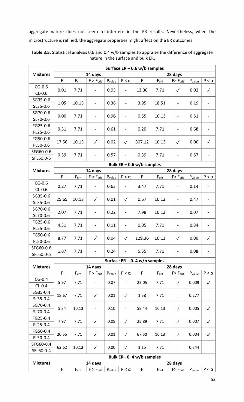
52

aggregate nature does not seem to interfere in the ER results. Nevertheless, when the

microstructure is refined, the aggregate properties might affect on the ER outcomes.

Table 3.5. Statistical analysis 0.6 and 0.4 w/b samples to appraise the difference of aggregate nature in the surface and bulk ER.

Mixtures

Surface ER – 0.6 w/b samples

14 days 28 days

F Fcrit F > Fcrit Pvalue P < α F Fcrit F> Fcrit Pvalue P < α

CG-0.6 0.01 7.71 - 0.93 - 13.30 7.71 ✓ 0.02 ✓

CL-0.6

SG35-0.6 1.05 10.13 - 0.38 - 3.95 18.51 - 0.19 -

SL35-0.6

SG70-0.6 0.00 7.71 - 0.96 - 0.55 10.13 - 0.51 -

SL70-0.6

FG25-0.6 0.31 7.71 - 0.61 - 0.20 7.71 - 0.68 -

FL25-0.6

FG50-0.6 17.56 10.13 ✓ 0.02 ✓ 807.12 10.13 ✓ 0.00 ✓

FL50-0.6

SFG60-0.6 0.39 7.71 - 0.57 - 0.39 7.71 - 0.57 -

SFL60.0-6

Mixtures

Bulk ER – 0.6 w/b samples

14 days 28 days


CG-0.6 0.27 7.71 - 0.63 - 3.47 7.71 - 0.14 -

CL-0.6

SG35-0.6 25.65 10.13 ✓ 0.01 ✓ 0.67 10.13 - 0.47 -

SL35-0.6

SG70-0.6 2.07 7.71 - 0.22 - 7.98 10.13 - 0.07 -

SL70-0.6

FG25-0.6 4.31 7.71 - 0.11 - 0.05 7.71 - 0.84 -

FL25-0.6

FG50-0.6 8.77 7.71 ✓ 0.04 ✓ 129.36 10.13 ✓ 0.00 ✓

FL50-0.6

SFG60-0.6 1.87 7.71 - 0.24 - 5.55 7.71 - 0.08 -

SFL60.0-6

Mixtures

Surface ER – 0. 4 w/b samples

14 days 28 days


CG-0.4 5.97 7.71 - 0.07 - 22.05 7.71 ✓ 0.009 ✓

CL-0.4

SG35-0.4 18.67 7.71 ✓ 0.01 ✓ 1.58 7.71 - 0.277 -

SL35-0.4

SG70-0.4 5.34 10.13 - 0.10 - 58.44 10.13 ✓ 0.005 ✓

SL70-0.4

FG25-0.4 7.97 7.71 ✓ 0.05 ✓ 25.89 7.71 ✓ 0.007 ✓

FL25-0.4

FG50-0.4 20.55 7.71 ✓ 0.01 ✓ 67.50 10.13 ✓ 0.004 ✓

FL50-0.4

SFG60-0.4 62.62 10.13 ✓ 0.00 ✓ 1.15 7.71 - 0.344 -

SFL60.0-4

Mixtures

Bulk ER– 0. 4 w/b samples

14 days 28 days


53

CG-0.4 7.50 7.71 - 0.05 - 29.71 7.71 ✓ 0.01 ✓

CL-0.4

SG35-0.4 0.27 7.71 - 0.63 - 3.48 7.71 - 0.14 -

SL35-0.4

SG70-0.4 24.39 10.13 ✓ 0.02 ✓ 21.80 10.13 ✓ 0.02 ✓

SL70-0.4

FG25-0.4 0.36 7.71 - 0.58 - 7.38 7.71 - 0.05 -

FL25-0.4

FG50-0.4 11.38 7.71 ✓ 0.03 ✓ 22.48 7.71 ✓ 0.01 ✓

FL50-0.4

SFG60-0.4 22.84 10.13 ✓ 0.02 ✓ 4.44 7.71 - 0.10 -

SFL60.0-4

Mixtures with 0.4 w/b resulted in higher ER when compared to w/b 0.6, as presented in the

results’ section; the latter indicates an enhancement of the inner quality of concrete

microstructure. Thus, it is interesting to notice that the surface ER results for these mixtures

(Table 3.5) presented a statistical significance regarding the coarse aggregate for most of them

(8 out of 12 mixtures), except for control and 70% GGBS mixes at 14 days, and 35% GGBS and

ternary mixtures at 28 days. A similar trend is found for bulk ER with 0.4 w/b. However, in this

particular setup (bulk ER), the 25% fly ash and 35% slag (14 days) mixtures presented no statistical

significance between the two coarse aggregates used, whereas for the 70% GGBS mixtures at 14

days the coarse aggregate was considered significant in the bulk ER and not significant in the

surface ER. This indicates that the influence of the coarse aggregate also depends on the test

setup.

Overall, the results gathered in this research and the statistical analysis presented in Table 1.5

are very coherent; granite is an igneous rock and usually displays higher density along with lower

absorption and porosity when compared to limestone (sedimentary rock) [51]. Hence, concrete

mixtures made of granite are expected to yield higher ER values, regardless of the test setup. This

trend is more pronounced for concrete mixtures presented refined microstructure (i.e. the more

advanced the hydration process and SCM’s replacement ratio, the more pronounced the

differences between concrete mixtures incorporating distinct aggregates). This outcome agrees

with the studied performed by [18]. Influence of the binder type on concrete ER.

3.6.2.2. Influence of binder type on concrete ER

Analyzing the fly ash influence on concrete ER results (Figure 3.4 to Figure 3.6), it is evident that

mixtures containing fly ash presented a delayed ER development, which rapidly evolved after 14

days. This has been observed because fly-ash is a pozzolan with very low CaO content; thus, it

first requires portlandite (CaOH2) to be formed in the system during PC hydration to subsequently

trigger the so-called “pozzolanic reaction”, which enhances the inner quality of the concrete

microstructure due to C-S-Hp formation. Fly ash is also known to present enhanced PSD, which

may improve the overall porosity of the system due to filler effect [52]. Finally, it is worth noting

54

that the delayed ER increment on the fly ash mixtures is in accordance with past researches

regarding fly-ash Class-F and ER outcomes [32,53].

Concrete mixtures made of GGBS also quite influenced on the concrete ER, especially after 14

days where one could notice that control mixtures presented a slower ER development when

compared to GGBS mixes. As highlighted in the literature by [54], a binary mixture made of PC

and GGBS tends to have a longer hydration kinetics and thus delays the development of C-S-H.

Lastly, GGBS might also increase concrete pore solution ER due to a reduction of alkali content

on the concrete pore solution [43].

In summary, all SCMs mixtures presented an important impact on the ER results over time. All

SCMs made mixes yielded higher ER values at 28 days when compared to control mixtures

indicating an improvement in the concrete microstructure over time. The latter took place mainly

due to the so-called pozzolanic and filler effects, which enhanced the materials microstructure,

reducing porosity [32,38,50,52,54]. Furthermore, the use of SCMs might also change the concrete

pore solution composition, reducing its alkalinity and thus improving resistivity as observed by

[9,41,55].

3.6.3. Forecasting compressive strength through the use of ER

As mentioned before, the surface and internal ER are the two most appealing test setups to be

used in the field. Therefore, this section studies the prediction of compressive strength through

surface and internal ER for mixes containing distinct binders and aggregate natures. To improve

the accuracy in early ages, the models were developed based on four concrete ER data points for

each setup and four compressive strength data points at distinct ages (i.e. 3, 7, 14, and 28 days);

except for 50% fly ash samples and ternary mixtures with 0.6 w/b, in which 3-day compressive

strength was not possible to measure since the samples were not hardened enough to be

demolded. Therefore, only 3 data points (i.e. 7, 14 and 28 days) were used to develop the models

of mixtures FG50-0.6, FG50-0.6, SFG60-0.6, and SFL60-0.6. Additionally, all the compressive

strength models are based on surface ER and Internal ER followed the least square method with

a logarithm relationship as presented in Equation 3.3.

𝑓`𝑐 = b ∗ log(concrete ER) + c Equation 3.3

55

a)

b)

c)

d)

Figure 3.10. Relationship between compressive strength and surface (a) 0.6 w/b mixtures and b) 0.4 w/b mixtures; and internal ER (c) 0.6 w/b mixtures and d) 0.4 w/b mixture) used to determine logarithm parameters.

The logarithm parameters calculated for each mixture investigated through Figure 3.10 are

presented in Table 3.6. For all the cases, the greater is the amount of SCM replaced, the smaller

the curve slope (a). However, it is worth noting that the ternary mixtures (SFG60 and SFL60)

presented a higher “b-parameter” than mixtures with higher percentage of SCMs, resulting in

steeper correlation. Additionally, all curves presented a reliable R² ranging from 0.75 to 1.00.

0

10

20

30

40

50

0.1 1.4 20.8 300.0

f’c

(MP

a)

Surface ER (kΩ.cm)

CG-0.6 CL-0.6 FG25-0.6 FL25-0.6

FG50-0.6 FL50-0.6 SG35-0.6 SL35-0.6

SG70-0.6 SL70-0.6 SFG60-0.6 SFL60-0.6

0

10

20

30

40

50

0.1 1.4 20.8 300.0

f’c

(MP

a)Surface ER (kΩ.cm)

CG-0.4 CL-0.4 FG25-0.4 FL25-0.4

FG50-0.4 FL50-0.4 SG35-0.4 SL35-0.4

SG70-0.4 SL70-0.4 SFG60-0.4 SFL60-0.4

0

10

20

30

40

50

0.1 1.4 20.8 300.0

f’c

(MP

a)

Internal ER (kΩ.cm)

CG-0.6 CL-06 FG25-0.6 FL25-0.6

FG50-0.6 FL50-0.6 SG35-0.6 SL35-0.6

SG70-0.6 SL70-0.6 SFG60-0.6 SFL60-0.6

0

10

20

30

40

50

0.1 1.4 20.8 300.0

f’c

(MP

a)

Internal ER (kΩ.cm)

CG-0.4 CL-0.4 FG25-0.4 FL25-0.4

FG50-0.4 FL50-0.4 SG35-0.4 SL35-0.4

SG70-0.4 SL70-0.4 SFG60-0.4 SFL60-0.4

56

Table 3.6. Regression parameters.

Mixtures 0.6 w/b 0.4 w/b

Internal ER Surface ER Internal ER Surface ER b c b c b c b c

CG 42.68 17.28 46.67 -11.58 23.46 27.50 33.22 14.26 CL 47.78 15.06 46.49 -9.05 21.73 25.76 30.48 15.20

SG35 18.67 12.85 20.58 -4.13 26.78 5.45 21.16 -2.73 SL35 13.93 12.09 19.71 -3.44 20.50 6.57 23.46 -6.60 SG70 8.43 0.13 9.81 -7.50 8.50 2.49 9.13 -3.42 SL70 8.23 -0.36 9.24 -7.13 7.12 3.69 16.07 -18.68 FG25 17.85 11.68 19.37 0.54 18.65 18.38 19.32 6.71 FL25 13.91 12.65 15.49 3.37 16.59 21.73 20.24 8.69 FG50 11.83 3.30 14.96 -6.30 14.16 4.81 16.03 -5.71 FL50 9.93 3.83 11.99 -3.89 12.84 5.15 12.99 -3.05

SFG60 15.24 2.55 9.83 -4.40 15.90 -2.78 12.10 -0.89 SFL60 17.10 0.60 12.45 -7.18 13.57 -0.79 14.90 -5.19

Regarding 0.6 w/b compressive strength prediction models (Figure 3.10a and c), as both

compressive strength and ER were not statically significant regarding the coarse aggregate

nature, similar behavior can be observed on the models, as expected. The absolute average

difference between predicted compressive strength for granite and limestone mixtures is 6.15%

(surface ER) and 8.81% (internal ER), respectively. The most important difference regarding the

coarse aggregate nature for 0.6 w/b mixtures for models using surface ER (Figure 3.10a) was

yielded by control samples (12.84%) at 7 days, whereas for models based on internal ER (Figure

3.10c), the greatest difference was obtained for ternary mixtures at 14 days (23.08%).

Furthermore, addressing 0.4 w/b models based on surface setup (Figure 3.10b), one may notice

that concrete mixtures in which the aggregate nature was considered statistically significant in

Table 3.5 (i.e. control samples, 70% GGBS, 25% fly-ash, 50% fly-ash replacement) also presented

the highest difference on compressive strength prediction (up to 38.33% at 7 days for 70% GGBS

mixtures). For these mixtures, both shape and R² were affected by the coarse aggregate nature;

for instance, it can be noticed that the shape of the curves of SG70-0.4 and SL70-0.4 (Figure 3.10b

square blue marker) changed dramatically. In addition, the “b-parameter” was modified from

9.13 to 16.07. This may prevent a proper early age prediction through the use of ER if the coarse

aggregate nature is not taking into consideration. Therefore, it is possible to conclude that the

coarse aggregate nature displays a quite significant role on ER results, especially when the

concrete microstructure is enhanced through the use of SCMs and/or reduced w/b ratios.

Regarding 0.4 w/b models applying internal ER (Figure 3.10d), the coarse aggregate impact was

not as significant as for surface ER. The highest difference concerning the influence of the coarse

aggregate nature on the compressive strength prediction was 16.91% (70% slag mixtures at 14

days), while the average difference is around two times smaller when compared to surface ER.

This indicates that depending on the setup, the coarse aggregate nature can be more or less

influential on the compressive strength prediction. Further analysis is still required to validate

this research finding based on a wider range of coarse aggregate natures.

57

3.6.3.1. Influence of binder type on concrete ER

a)

b)

Figure 3.11. Analysis of experimental-to-predicted compressive strength ratio predicted through surface ER: a) 0.6 w/b mixtures; b) 0.4 w/b mixtures.

All 0.6 w/b predictions models resulted in an average error of 6.81% (Figure 3.11a). This indicates

that the variability observed in the results seems to come from other factors such as concrete

heterogeneity itself. Moreover, one may notice that the ternary mixture (red triangle) presented

higher variation of the experimental-to-predicted ratio; this might have occurred due to the high

amounts of two different SCMs (fly ash and slag) used, which demands more time to develop

hardening products due to delayed pozzolanic reactions. Furthermore, analyzing the predicted

compressive strength (f’c) of 0.4 w/b mixtures (Figure 3.11b), the average error between

predicted compressive strength and measured compressive strength for at all ages is 12.46%.

However, the f’c prediction error (1.56) can be also noticed for ternary mixtures at 7 days, as

expected based on 0.6 w/b results. Yet, the results are more scattered for 0.4 w/b mixtures than

0.6 w/b mixes.

Figure 3.12 presents the experimental-to-predicted compressive strength ratio forecasted

through internal ER. 0.6 w/b (Figure 3.12a) mixtures yielded a prediction average error for all the

mixtures at all ages of 9.60%. These values are in accordance with surface ER 0.6 w/b prediction

models (6.81%). Yet, surface ER 0.6 w/b (Figure 3.11a) mixtures resulted in slightly more precise

prediction models as the data are closer to the target line 1.00. Furthermore, analyzing 0.4 w/b

mixtures (Figure 3.11b and Figure 3.12b), one may see that, the average error for internal ER

setup models was 4.09%, while for surface ER it was 12.46%. Therefore, internal ER yielded more

appealing prediction models. Lastly, the mean prediction ratio for all families within all ages and

w/b is 1.00 with a standard deviation of 0.11 for all setups, being the most accurate method.

0.00

0.50

1.00

1.50

2.00

0 10 20 30 40 50

Exp

erim

en

tal-

to-p

red

icte

d r

atio

Measured Strength (MPa)

CG0.6 CL0.6 FG25-0.6 FL25-0.6

FG50-0.6 FL50-0.6 SG35-0.6 SL35-0.6

SG70-0.6 SL70-0.6 SFG60-0.6 SFL60-0.6

0.00

0.50

1.00

1.50

2.00

0 10 20 30 40 50

Exp

erim

en

tal-

to-p

red

icte

d r

atio


CG0.4 CL0.4 FG25-0.4 FL25-0.4

FG50-0.4 FL50-0.4 SG35-0.4 SL35-0.4

SG70-0.4 SL70-0.4 SFG60-0.4 SFL60-0.4

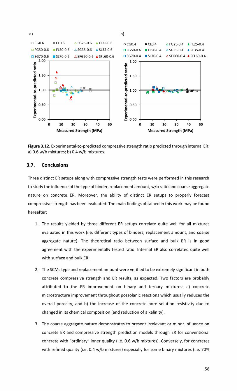
58

a)

b)

Figure 3.12. Experimental-to-predicted compressive strength ratio predicted through internal ER: a) 0.6 w/b mixtures; b) 0.4 w/b mixtures.

3.7. Conclusions

Three distinct ER setups along with compressive strength tests were performed in this research

to study the influence of the type of binder, replacement amount, w/b ratio and coarse aggregate

nature on concrete ER. Moreover, the ability of distinct ER setups to properly forecast

compressive strength has been evaluated. The main findings obtained in this work may be found

hereafter:

1. The results yielded by three different ER setups correlate quite well for all mixtures

evaluated in this work (i.e. different types of binders, replacement amount, and coarse

aggregate nature). The theoretical ratio between surface and bulk ER is in good

agreement with the experimentally tested ratio. Internal ER also correlated quite well

with surface and bulk ER.

2. The SCMs type and replacement amount were verified to be extremely significant in both

concrete compressive strength and ER results, as expected. Two factors are probably

attributed to the ER improvement on binary and ternary mixtures: a) concrete

microstructure improvement throughout pozzolanic reactions which usually reduces the

overall porosity, and b) the increase of the concrete pore solution resistivity due to

changed in its chemical composition (and reduction of alkalinity).

3. The coarse aggregate nature demonstrates to present irrelevant or minor influence on

concrete ER and compressive strength prediction models through ER for conventional

concrete with “ordinary” inner quality (i.e. 0.6 w/b mixtures). Conversely, for concretes

with refined quality (i.e. 0.4 w/b mixtures) especially for some binary mixtures (i.e. 70%

0.00

0.50

1.00

1.50

2.00

0 10 20 30 40 50

Exp

erim

en

tal-

to-p

red

icte

d r

atio


CG0.6 CL0.6 FG25-0.6 FL25-0.6

FG50-0.6 FL50-0.6 SG35-0.6 SL35-0.6

SG70-0.6 SL70-0.6 SFG60-0.6 SFL60-0.6

0.00

0.50

1.00

1.50

2.00

0 10 20 30 40 50Ex

per

ime

nta

l-to

-pre

dic

ted

raa

tio


CG0.4 CL0.4 FG25-0.4 FL25-0.4

FG50-0.6 FL50-0.4 SG35-0.4 SL35-0.4

SG70-0.4 SL70-0.4 SFG60-0.4 SFL60-0.4

59

GGBS and 50% fly-ash replacement), the coarse aggregate nature was seen to impact on

the ER results. The latter has been proven statistically.

Concrete compressive strength can be accurately predicted through surface or internal ER, when

the prediction model accounts for the binder type and amount along with the coarse aggregate

nature. However, the results show that the internal ER is the most accurate method to predict

the compressive strength of conventional concrete incorporating single, binary and ternary

binder blends.

3.8. References

[1] K. L. Scrivener and R. J. Kirkpatrick, “Innovation in use and research on cementitious

material,” Cem. Concr. Res., vol. 38, no. 2, pp. 128–136, 2008, doi:

10.1016/j.cemconres.2007.09.025.

[2] M. S. Ali, E. Leyne, M. Saifuzzaman, and M. S. Mirza, “An experimental study of

electrochemical incompatibility between repaired patch concrete and existing old concrete,”

Constr. Build. Mater., vol. 174, pp. 159–172, 2018, doi: 10.1016/j.conbuildmat.2018.04.059.

[3] S. Mirza, “Durability and sustainability of infrastructure — a state-of-the-art report 1,” vol.

649, pp. 639–649, 2006, doi: 10.1139/L06-049.


Mater. J., pp. 1–52, 2019.

[5] R. H. Elvery and L. A. M. Ibrahim, “Ultrasonic assessment of concrete strength at early

ages,” Mag. Concr. Res., vol. 28, no. 97, pp. 181–190, Jun. 1976, doi:

10.1680/macr.1976.28.97.181.

[6] T. R. Naik and B. W. Ramme, “Determination of the water content of concrete by the

microwave method,” Cem. Concr. Res., vol. 17, no. 6, pp. 927–938, 1987, doi: 10.1016/0008-

8846(87)90081-0.

[7] M. Nagi and D. Whiting, “Determination of water content of fresh concrete using a

microwave oven,” Cem. Concr. Aggregates, vol. 16, no. 2, pp. 125–131, 1994, doi:

10.1520/cca10290j.



10.1061/(ASCE)0899-1561(2006)18:1(99).



Oct. 2010, doi: 10.14359/51664045.

60

[10] R. M. Ferreira and S. Jalali, “NDT measurements for the prediction of 28-day compressive

strength,” NDT E Int., vol. 43, no. 2, pp. 55–61, 2009, doi: 10.1016/j.ndteint.2009.09.003.

[11] J. A. Bogas, M. G. Gomes, and A. Gomes, “Compressive strength evaluation of structural

lightweight concrete by non-destructive ultrasonic pulse velocity method,” Ultrasonics, vol. 53,

no. 5, pp. 962–972, 2013, doi: 10.1016/j.ultras.2012.12.012.


[13] O. Mohamed and O. Najm, “Effect of Curing Methods on Compressive Strength of

Sustainable Self-Consolidated Concrete,” IOP Conf. Ser. Mater. Sci. Eng., vol. 471, no. 3, 2012,

doi: 10.1088/1757-899X/471/3/032059.

[14] J.-K. Kim, Y.-H. Moon, and S.-H. Eo, “Compressive Strength Development of Concrete

With,” Compressive Strength Dev. Concr. With Differ. Curing Time Temp., vol. 28, no. 12, pp.

1761–1773, 1998.


electrical resistivity measurements in cementitious systems,” Transp. Res. Rec., no. 2342, pp.

90–98, 2013, doi: 10.3141/2342-11.

[16] P. J. Tumidajski, A. S. Schumacher, S. Perron, P. Gu, and J. J. Beaudoin, “On the

Relationship between Porotisy and Electrical Resistivity in Cementitious systems,” Cem. Concr.

Res., vol. 26, no. 4, pp. 539–544, 1996.



10.1002/maco.201005777.



5533.0002661.



10.1155/2014/742129.



10.1016/j.conbuildmat.2011.12.111.

[21] L. Xiao and X. Wei, “Early age compressive strength of pastes by electrical resistivity

method and maturity method,” J. Wuhan Univ. Technol. Mater. Sci. Ed., vol. 26, no. 5, pp. 983–

989, 2011, doi: 10.1007/s11595-011-0349-3.

61



Oct. 2010, doi: 10.14359/51664045.

[23] R. B. Polder, “Test methods for on site measurement of resistivity of concrete a RILEM TC-

154 technical recommendation,” p. 7, 2001.


determine initial setting time of cement and concrete using plate test,” Mater. Struct., vol. 49,

no. 8, pp. 3135–3142, Oct. 2016, doi: 10.1617/s11527-015-0709-0.

[25] AASHTO, “Standard test method for surface resistivity of concrete`s ability to resist

chloride ion penetration.,” AASTHO TP95, vol. Washigton, p. DC: AASHTO., 2014.

[26] ASTM C1876, “Standard Test Method for Bulk Electrical Conductivity of Hardened

Concrete,” pp. 1–5, 2012, doi: 10.1520/C1876-19.

[27] W. Elkey and E. J. Sellevold, “Electrical resistivity of concrete,” Nor. Road Res. Lab., p. 33,

1995.

[28] H. Layssi, P. Ghods, A. R. Alizadeh, and M. Salehi, “Electrical Resistivity of Concrete,” p. 6.

[29] A. Princigallo, K. van Breugel, and G. Levita, “Influence of the aggregate on the electrical

conductivity of Portland cement concretes,” Cem. Concr. Res., vol. 33, no. 11, pp. 1755–1763,

Sep. 2003, doi: 10.1016/S0008-8846(03)00166-2.

[30] M. A. M. Fadel, H. Zabidi, and K. S. Ariffin, “Monitoring the Quarry Pit Development,”

Procedia Chem., vol. 19, pp. 721–728, 2016, doi: 10.1016/j.proche.2016.03.076.

[31] P. Azarsa and R. Gupta, “Electrical Resistivity of Concrete for Durability Evaluation: A

Review,” Adv. Mater. Sci. Eng., vol. 2017, 2017, doi: 10.1155/2017/8453095.

[32] H. Yildirim, T. Ilica, and O. Sengul, “Effect of cement type on the resistance of concrete

against chloride penetration,” Constr. Build. Mater., vol. 25, no. 3, pp. 1282–1288, 2010, doi:

10.1016/j.conbuildmat.2010.09.023.

[33] Y. Liu and F. J. Presuel-Moreno, “Normalization of temperature effect on concrete

resistivity by method using Arrhenius law,” ACI Mater. J., vol. 111, no. 4, pp. 433–442, 2014, doi:

10.14359/51686725.

[34] P. K. Metha and P. J.M. Monteiro, Concrete Miscrostructure, Properties and Mateirals,

3rd ed. McGraw Hill, 2006.

[35] J. Lateste, D. Breysse, C. Sirieix, and S. Naar, “Electrical Resistivity Measurements on

Various Concretes Submitted to Marine Environments. Structural Faults and Repair,” p. 9, 2006.

62

[36] J. Hill and J. H. Sharp, “The mineralogy and microstructure of three composite cements

with high replacement levels,” Cem. Concr. Compos., vol. 24, no. 2, pp. 191–199, Sep. 2002, doi:

10.1016/S0958-9465(01)00041-5.

[37] P. Ghosh and Q. Tran, “Correlation Between Bulk and Surface Resistivity of Concrete,” Int.

J. Concr. Struct. Mater., vol. 9, no. 1, pp. 119–132, Sep. 2015, doi: 10.1007/s40069-014-0094-z.

[38] M. Nokken, A. Boddy, X. Wu, and R. D. Hooton, “Effects of temperature, chemical, and

mineral admixtures on the electrical conductivity of concrete,” J. ASTM Int., vol. 5, no. 5, pp. 1–

9, 2008, doi: 10.1520/JAI101296.

[39] K. H. Khayat, “Influence of Supplementary Cementitious Materials and Fillers on

Rheological Properties, Kinetics of Cement Hydration, and Compressive Strength of Concrete-

Equivalent Mortar of SCC... High-Volume Recycled Materials for Sustainable Pavement

Construction Vi,”, pp. 382-392 2010.


Technique Affairs in partial fulfillment of the requirements for the degree of Master of Applied

Science,”p. 200, 2015.

[41] D. P. Bentz, K. A. Snyder, and A. Ahmed, “Anticipating the setting time of high-volume fly

ash concretes using electrical measurements: Feasibility studies using pastes,” J. Mater. Civ. Eng.,

vol. 27, no. 3, 2015, doi: 10.1061/(ASCE)MT.1943-5533.0001065.

[42] Y. Bu and J. Weiss, “The influence of alkali content on the electrical resistivity and

transport properties of cementitious materials,” Cem. Concr. Compos., vol. 51, pp. 49–58, 2014,

doi: 10.1016/j.cemconcomp.2014.02.008.

[43] Q. Zhao, J. Stark, E. Freyburg, and M. Zhou, “the Mechanism of Gbfs Preventing Aar : a

Discussion,” 13th Int. Conf. Alkali-Aggregate React. Concr., p. 11, 2008.

[44] CAN/CSA-A3000-13, “Cementitious Materials Compendium,” 2013.

[45] ASTM C150/C150M, “Standard Specification for Portland Cement,” pp. 1–10, 2019, doi:

10.1520/C0150.

[46] ASTM C618, “Standard Specification for Coal Fly Ash and Raw or Calcined Natural Pozzolan

for Use,” pp. 1–5, 2019, doi: 10.1520/C0618-19.2.

[47] Giatec, “SmartBox,” 2020. [Online]. Available:

https://www.giatecscientific.com/products/concrete-sensors/smartbox-electrical-resistivity/.

[Accessed: 15-Mar-2020].

[48] ASTM C33, “Standard test method for sieve analysis of fine and coarse aggregates.,” p. 8,

2016.

63

[49] ASTM C39/C39M, “Standard Test Method for Compressive Strength of Cylindrical

Concrete Specimens,” pp. 1–8, 2020, doi: 10.1520/C0039.

[50] P. Ghosh and Q. Tran, “Correlation Between Bulk and Surface Resistivity of Concrete,” Int.

J. Concr. Struct. Mater., vol. 9, no. 1, pp. 119–132, 2015, doi: 10.1007/s40069-014-0094-z.

[51] F. Pacheco Torgal and J. P. Castro-Gomes, “Influence of physical and geometrical

properties of granite and limestone aggregates on the durability of a C20/25 strength class

concrete,” Constr. Build. Mater., vol. 20, no. 10, pp. 1079–1088, 2006, doi:

10.1016/j.conbuildmat.2005.01.063.

[52] N. Bouzoubaâ, M. H. Zhang, V. M. Malhotra, and D. M. Golden, “Blended fly ash cements

- A review,” ACI Mater. J., vol. 96, no. 6, pp. 641–650, 1999, doi: 10.14359/789.

[53] M. Nokken, A. Boddy, X. Wu, R. D. Hooton, D. Hooton, and S. W. Dean, “Effects of

Temperature, Chemical, and Mineral Admixtures on the Electrical Conductivity of Concrete,” J.

ASTM Int., vol. 5, no. 5, p. 101296, Nov. 2008, doi: 10.1520/JAI101296.

[54] W. Chen, Hydration of slag cement. Theory, modeling and application., p. 241,2007.


Technique,” p. 200, 2015.

64

4. Chapter Four: Conclusion and future recommendations

Electrical Resistivity is an inexpensive, fast, and reliable non-destructive technique able to

characterize the cementitious materials’ hydration process and predict compressive strength in

the field, which allows a fast and accurate surveying of the entire structure at minimum cost. Yet,

recent literature data have evidenced that ER might be significantly influenced by a variety of

parameters, such as the supplementary cementing materials (SCM) type/amount and aggregates

nature (i.e. minerology) used in the mix. These factors can hinder the practical benchmark of

concrete mixtures proportioned with distinct raw materials. Therefore, three different ER setups

(surface ER, bulk ER, and Internal ER) along with compressive strength tests were conducted in

this research to evaluate the influence of the type of binder and replacement amount along with

the coarse aggregate’s nature on concrete ER development and compressive strength prediction.

The main findings obtained in this work may be found hereafter:

1. The results generated from 3 different ER configurations correlate fairly well for different

types of binders, replacement ratio, and coarse aggregate nature. The experimental ratio

between surface and bulk ER is in great concordance with the hypothetical ratio. Internal

ER also correlated fairly well with surface and bulk ER indicating that electrical resistivity

is, in fact, an intrinsic characteristic of cementitious materials such as concrete.

2. The SCMs category and replacement ratio has demonstrated to enormously influence on

concrete ER and compressive strength, as previously reported in the literature. Two

factors are probably attributed to the ER enhancement on the binary and ternary

concrete mixtures, which are: a) concrete microstructure improvement throughout

pozzolanic reactions which typically reduces pores sizes decreasing overall permeability

and, b) the growth of concrete pore solution ER due to modifications in the chemical

composition and ions concentration of the concrete pore solution.

3. The coarse aggregate nature has been verified to be irrelevant or displaying a minor role

on concrete ER and compressive strength models for “ordinary concrete” concrete

mixtures (i.e. 0.6 w/c mixtures). Conversely, for concrete mixes with enhanced inner

quality (i.e. 0.4 w/c samples), especially for binary mixtures (i.e. 70% GGBS, 25% fly-ash,

and 50% fly-ash replacement), the coarse aggregate nature was found to be statically

significant for ER outcomes and compressive strength predictions. Yet, further analyses

are essential to further understand and validate the results obtained in this research.

4. ER has shown to be a quite reliable NDT, able to predict compressive strength until 28

days regardless of the SCMs type and replacement amount. Furthermore, in this

particular research, internal ER results demonstrated to be the most reliable to forecast

compressive strength of single, binary and ternary mixtures.

65

Although important data has been gathered in this research, which enhanced the current

knowledge in the field, further investigations could be performed for a deeper understanding of

some of the research findings, as presented hereafter:

The influence of the chemistry of the concrete pore solution in both fresh and hardened

states on concrete ER is still required to understand how the distinct SCMs types and

replacement ratios are impacting on the overall ER outcomes.

Microscopic and thermographic analysis on paste samples made of the same SCMs

type/amount to understand how the formation of distinct hydration products impact on

ER.

Porosity analysis on concrete samples to determine how different coarse aggregate

natures combined with distinct SCMs type/amount are impacting on the overall concrete

microstructure (i.e. porosity), and thus ER outcomes

An evaluation of the impact of the aggregate electrical properties and physical features

(shape and texture) on the overall concrete microstructure (i.e. porosity), and thus ER.

An extended research with a wider range of coarse aggregate natures (displaying distinct

lithotypes), water-to-binder ratios and SCMs type/amount would be beneficial to validate

and improve the relationships and models gathered and proposed in this research.

66

1. Chapter Five: Appendix

5.1. Introduction

Based on the thesis findings, the aggregate lithotype combined with the binder type/amount and

the water-to-binder ratio may significantly impact on the concrete ER results. Therefore, two

distinct assumptions were drawn to clarify such an impact: a) enhancement in concrete

microstructure due to the decrease of the water-to-binder ratio and thus porosity and, b)

increase in ER due to the change in the chemistry of pore solution while the use of SCMs. To

evaluate the first assumption, the assessment of the concrete capillary porosity was conducted.

Likewise, to appraise the second, the pore solution extraction on fresh pastes incorporating

distinct SCMs types and amounts was performed.

5.2. Materials and Methods

In this section, further details on the experiments to analyze the above assumptions are

presented. For the porosity evaluations, a total of 24 mixtures presenting two coarse aggregate

types (i.e. granite - igneous rock and limestone - sedimentary rock) from Ontario and Quebec

(Canada), and displaying two w/b (e.g. 0.6 and 0.4) were selected. Two types of SCMs (i.e. fly ash

and slag) were used in some mixes as a partial replacement (in mass) of a conventional Portland

cement GU type. Two levels of replacement were selected for each SCM selected (e.g. 35%, 70%

- slag, 25%, 50% fly-ash, and, 35% slag and 25% fly-ash for a ternary mix) based on Table 9 of CSA

A3001-13 [1]. Likewise, a total of 12 pastes mixtures were prepared according to ASTM C305 [2]

with the same SCM replacement for the fresh state pore solution extraction.

5.2.1. Porosity test

The concrete cylinders were sliced radially in three similar samples at 28 days (Figure 5.1a) using

a diamond blade. Moreover, the samples were oven dried for 15 days at 0% relative humidity

and 60 ͦC until they reached a constant dry-mass (md). The samples were then submerged in

water for 24 hours and a pressure of 760 mmHg was applied, using a vacuum pump (Figure 5.1b).

Finally, the samples were measured at both submerged (ms, using a submerged basket) and

surface saturated dry condition (mssd).

67

a)

b) .

Figure 5.1. a) Samples Cutting Scheme; b) Porosity Test Setup.

Finally, according to ASTM C127 [3], it was possible to determine the Apparent Porosity (AP; or

capillary porosity) using the Equation 5.1.

𝐴𝑃 =𝑚𝑠𝑠𝑑 − 𝑚𝑑

𝑚𝑠𝑠𝑑 − 𝑚𝑠

Equation 5.1

5.2.2. Fresh state pore solution extraction

Thirty minutes after casting, the pore solution (i.e. liquid phase) extraction was performed

applying a constant pressure at 600 mmHg using a vacuum pump. Moreover, an Erlenmeyer flask

with a side port, a funnel, a sealing rubber and 2 filter papers with pore size of 20-25 μm (i.e., the

larger with 185 mm diameter to cover the entire internal funnel wall and confine the paste

sample, and the smaller with 50 mm diameter at the bottom of the funnel to avoid tearing up as

a result of stress concentrations) were used in the setup (Figure 5.2) to perform the pore solution

extraction. The suction/extraction process lasted around 6 minutes on average for collecting

about 20 ml of pore solution; yet, it highly depended on the w/b of the paste samples.

Additionally, the pore solution ER and its pH (right after the extraction) were measured using a

conductivity meter and a pH meter respectively. The pore solutions were stored in plastic tubes

with air-tight lids to prevent carbonation and other forms of contamination and an Inductively

Coupled Plasma Emission Spectroscopy (ICP-ES) was performed to determine the chemistry pf

the pore solution.

Figure 5.2. Fresh state pore solution extraction setup.

68

5.2.3. Pore Solution ICP-ES analysis

The ICP-ES analysis provides the main cations concentration in mol/L from the pastes pore

solutions (i.e., Ca2+, K+, Na+, S+). Yet, to determine the main respective anions (OH-, SO4-2), some

further calculations should be performed.

To determine the SO4-2 concentration, stoichiometry calculation has been developed based on

the S+ concentration from the ICP-ES data. Therefore, by simply multiplying the S+ concentration

from the ICP-ES results with ratio between the respective atomic masses of the two molecules

(S+ and SO4-2) is possible to determine the SO4

-2 concentration in mol/L in the pore solution.

Moreover, to determine the OH- concentration in the pastes pore solution, an electrical charge

balance between the main cations and anion concentrations in mol/L was performed based on

Equation 5.2 [4].

[𝑂𝐻−] = [𝑁𝑎+] + [𝐾+] + 2[𝐶𝑎2+] − 2[𝑆𝑂4−2] Equation 5.2

5.3. Results

The AP and pore solution ER, pH and ICP-ES results are presented in this section.

5.3.1. Apparent Porosity

Figure 5.3. gives a plot of the AP results of the distinct mixtures evaluated in this research at the

28 days.

a)

b)

Figure 5.3. Apparent Porosity Fresh at 28 days outcomes: a) 0.6 w/b mixtures; b) 0.4 w/b

mixtures.

0

3

6

9

12

15

18

CG

-0.6

CL-

0.6

FG2

5-0

.6

FL2

5-0

.6

FG5

0-0

.6

FL5

0-0

.6

SG3

5-0

.6

SL3

5-0

.6

SG7

0-0

.6

SL7

0-0

.6

SFG

60

-0.6

SFL6

0-0

.6

Ap

par

en

t P

oro

sity

(%

)

0

3

6

9

12

15

18

CG

-0.4

CL-

0.4

FG2

5-0

.4

FL2

5-0

.4

FG5

0-0

.4

FL5

0-0

.4

SG3

5-0

.4

SL3

5-0

.4

SG7

0-0

.4

SL7

0-0

.4

SFG

60

-0.4

SFL6

0-0

.4

Ap

par

ent

Po

rosi

ty (

%)

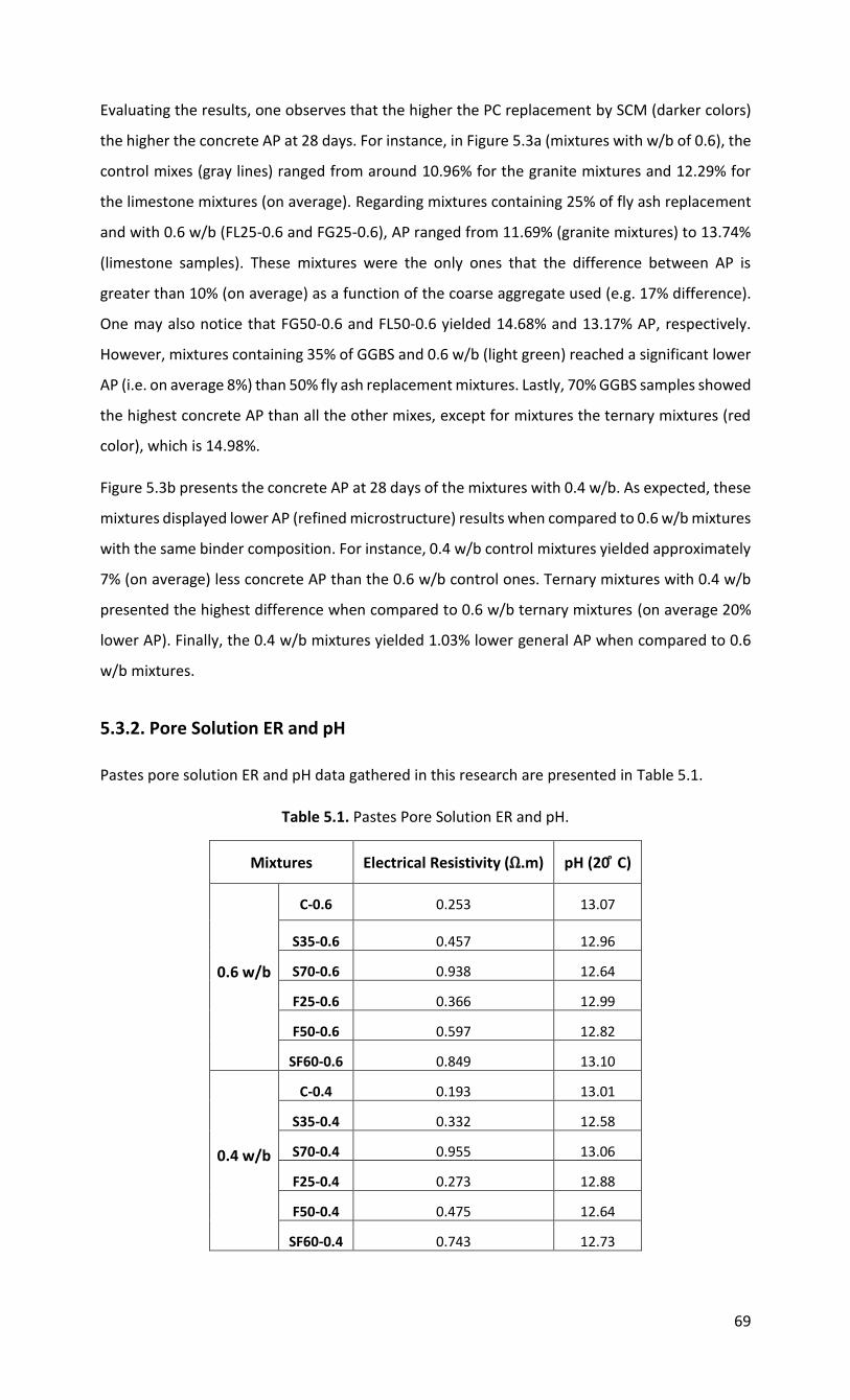
69

Evaluating the results, one observes that the higher the PC replacement by SCM (darker colors)

the higher the concrete AP at 28 days. For instance, in Figure 5.3a (mixtures with w/b of 0.6), the

control mixes (gray lines) ranged from around 10.96% for the granite mixtures and 12.29% for

the limestone mixtures (on average). Regarding mixtures containing 25% of fly ash replacement

and with 0.6 w/b (FL25-0.6 and FG25-0.6), AP ranged from 11.69% (granite mixtures) to 13.74%

(limestone samples). These mixtures were the only ones that the difference between AP is

greater than 10% (on average) as a function of the coarse aggregate used (e.g. 17% difference).

One may also notice that FG50-0.6 and FL50-0.6 yielded 14.68% and 13.17% AP, respectively.

However, mixtures containing 35% of GGBS and 0.6 w/b (light green) reached a significant lower

AP (i.e. on average 8%) than 50% fly ash replacement mixtures. Lastly, 70% GGBS samples showed

the highest concrete AP than all the other mixes, except for mixtures the ternary mixtures (red

color), which is 14.98%.

Figure 5.3b presents the concrete AP at 28 days of the mixtures with 0.4 w/b. As expected, these

mixtures displayed lower AP (refined microstructure) results when compared to 0.6 w/b mixtures

with the same binder composition. For instance, 0.4 w/b control mixtures yielded approximately

7% (on average) less concrete AP than the 0.6 w/b control ones. Ternary mixtures with 0.4 w/b

presented the highest difference when compared to 0.6 w/b ternary mixtures (on average 20%

lower AP). Finally, the 0.4 w/b mixtures yielded 1.03% lower general AP when compared to 0.6

w/b mixtures.

5.3.2. Pore Solution ER and pH

Pastes pore solution ER and pH data gathered in this research are presented in Table 5.1.

Table 5.1. Pastes Pore Solution ER and pH.

Mixtures Electrical Resistivity (Ω.m) pH (20 ͦC)

0.6 w/b

C-0.6 0.253 13.07

S35-0.6 0.457 12.96

S70-0.6 0.938 12.64

F25-0.6 0.366 12.99

F50-0.6 0.597 12.82

SF60-0.6 0.849 13.10

0.4 w/b

C-0.4 0.193 13.01

S35-0.4 0.332 12.58

S70-0.4 0.955 13.06

F25-0.4 0.273 12.88

F50-0.4 0.475 12.64

SF60-0.4 0.743 12.73

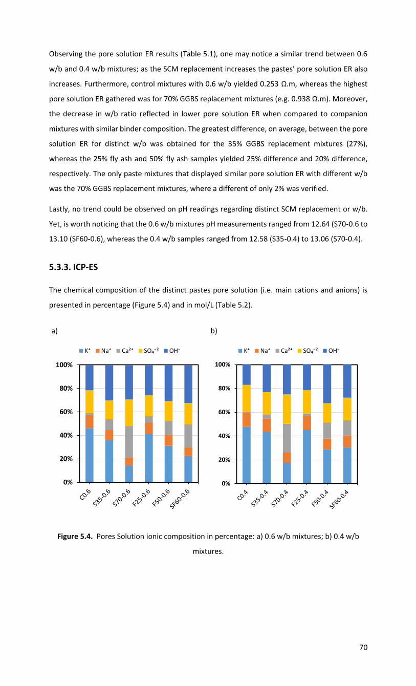
70

Observing the pore solution ER results (Table 5.1), one may notice a similar trend between 0.6

w/b and 0.4 w/b mixtures; as the SCM replacement increases the pastes’ pore solution ER also

increases. Furthermore, control mixtures with 0.6 w/b yielded 0.253 Ω.m, whereas the highest

pore solution ER gathered was for 70% GGBS replacement mixtures (e.g. 0.938 Ω.m). Moreover,

the decrease in w/b ratio reflected in lower pore solution ER when compared to companion

mixtures with similar binder composition. The greatest difference, on average, between the pore

solution ER for distinct w/b was obtained for the 35% GGBS replacement mixtures (27%),

whereas the 25% fly ash and 50% fly ash samples yielded 25% difference and 20% difference,

respectively. The only paste mixtures that displayed similar pore solution ER with different w/b

was the 70% GGBS replacement mixtures, where a different of only 2% was verified.

Lastly, no trend could be observed on pH readings regarding distinct SCM replacement or w/b.

Yet, is worth noticing that the 0.6 w/b mixtures pH measurements ranged from 12.64 (S70-0.6 to

13.10 (SF60-0.6), whereas the 0.4 w/b samples ranged from 12.58 (S35-0.4) to 13.06 (S70-0.4).

5.3.3. ICP-ES

The chemical composition of the distinct pastes pore solution (i.e. main cations and anions) is

presented in percentage (Figure 5.4) and in mol/L (Table 5.2).

a)

b)

Figure 5.4. Pores Solution ionic composition in percentage: a) 0.6 w/b mixtures; b) 0.4 w/b

mixtures.

0%

20%

40%

60%

80%

100%

K⁺ Na⁺ Ca²⁺ SO₄⁻² OH⁻

0%

20%

40%

60%

80%

100%

K⁺ Na⁺ Ca²⁺ SO₄⁻² OH⁻

71

Table 5.2. Pastes Pore Solution ionic composition in mol/L.

Mixtures Ca²⁺ K⁺ Na⁺ SO₄⁻² OH⁻

(mol/L)

0.6 w/b

C-0.6 0.007 0.218 0.053 0.092 0.102

S35-0.6 0.020 0.085 0.021 0.038 0.071

S70-0.6 0.023 0.012 0.006 0.019 0.025

F25-0.6 0.015 0.121 0.030 0.052 0.076

F50-0.6 0.021 0.053 0.015 0.029 0.052

SF60-0.6 0.027 0.031 0.010 0.026 0.045

0.4 w/b

C-0.4 0.006 0.311 0.078 0.146 0.111

S35-0.4 0.009 0.127 0.032 0.055 0.067

S70-0.4 0.022 0.017 0.008 0.023 0.023

F25-0.4 0.008 0.185 0.047 0.080 0.088

F50-0.4 0.023 0.050 0.016 0.028 0.056

SF60-0.4 0.018 0.043 0.014 0.027 0.039

Analyzing both Figure 5.4 and Table 5.2, one may notice that the SCM replacement and binder

type drastically influence on the chemical composition of the pore solution, as expected.

Furthermore, as the SCM replacement increases, the amount of Ca2+ also increases, whereas the

remaining main ions decrease with the incorporation of SCMs. For instance, the control mixtures

with 0.6 w/b presented 2% Ca2+ concentration, whereas the 70% GGBS samples yielded 27% Ca2+

concentration. Likewise, comparing fly ash samples with 0.6 w/b, the K+ concentration varied

from 41% (F25-0.6) to 31% (F50-0.6). This behavior was also clear while the analysis of OH- ions

concentration in mol/L (Table 5.2) between 35% GGBS replacement mixtures (0.071 mol/L) and

the ternary mixtures (0.045 mol/L).

Considering the w/b influence on the pore solution chemical composition, it is worth noting that

with the decrease of the pastes w/b, the ionic concentration increased for all the ions analyzed,

except Ca2+, as these mixtures present a higher amount of SCMs for a similar water amount. Thus,

comparing the OH- concentration in mol/L for control mixtures with different w/b, it is possible

to notice an 8% increase between C-0.6 and C-0.4. This difference is 13% when comparing the

samples with 25% fly ash replacement and different w/b. Additionally, comparing Na+

concentration of 35% GGBS mixtures with difference w/, a 34% increase is noticed, whereas for

70% GGBS mixtures, the difference was of 28%. Finally, analyzing ternary mixtures with different

w/b, one verifies that the Ca2+ concentration in mol/L decreased in -54% with the lessening of

w/b.

72

5.4. Discussion

5.4.1. Apparent Porosity

Analyzing the AP results (Figure 5.3) it is evident that the first assumption (i.e. the decrease in

w/b lessens the concrete capillary porosity) is true. Thus, concrete with lower w/b display indeed

a refined microstructure when compared to companion mixtures with same binder composition

and greater w/b. Therefore, concrete mixtures with different w/b might experience different

electrical conduction paths due distinct microstructure qualities and subsequently, the coarse

aggregate lithotype might be more influential in concrete mixture with refined microstructure

(lower w/b) when compared to mixes with higher w/b (and thus porosity).

5.4.2. SCM replacement influence on pastes Pore Solution

Calcium to Alkalis ratio SCM replacement influence

The ICP-ES analysis (Figure 5.4) clearly demonstrates that the SCM replacement increases the

Ca2+ while the other main ions concentration lessens. On one hand, analyzing the binder raw

composition (Table 3.3), it is evident that PC bears the greatest CaO concentration, while fly ash

presents the lowest CaO, followed by GGBS. Conversely, the higher the SCM content, the lower

less Ca2+ available in the pore solution, at least at early ages (i.e. 30 minutes after casting). There

are two probable explanations to this behaviour: a) Ca2+ ions display a limited solubility in high

pH media [5]. Thus, there is not enough time for all CaO to react with the water in the system; b)

SCMs replacement increases the nucleation process [6], which might speed up the Ca2+

dissolution in the pore solution. Furthermore, as mentioned before, the remaining main ions

increase their concentrations with the SCMs incorporation, especially alkalis cations (i.e. K+ and

Na+). However, analyzing the binders raw compositions (Table 3.3) it is evident that PC presents

the lowest amount Na2Oeq concentration, while fly ash has the highest amount, followed by

GGBS. Yet, the greater the SCMs replacement in system, the lower the alkalis ions present in the

pore solution. This can most likely be explained by the fact that SCMs usually require sub-

products from PC hydration to be formed (i.e. Portlandite) so that pozzolanic reactions are

triggered, releasing thus alkalis to the system [7-9]. Hence, as the alkalis concentration decreases

and the calcium concentration raises with the increase of SCM replacement, the Ca2+ to alkalis

(i.e. K+ and Na+) ratio can be determined. Analyzing the relationships between this experimental

ratio and OH- ions concentration (Figure 5.5), it is evident that the higher the SCM replacement,

the higher the calcium to alkalis ratio also.

73

Figure 5.5. Ca2+/(k++ Na+) ratio and OH- ion concentration correlation.

Observing Figure 5.5, it is possible to observe two clear and distinct logarithmic trends between

the calcium to alkalis ratio and the hydroxyl ion concentration on the pastes pore solution for

each w/b ratio studied in this research. Yet, for hydroxyl concentration values above and beyond

0.06 mol/L, the two curves are very close to each other; these mixtures are the ones with SCMs

replacement ratios above 35%. Furthermore, is worth noting that most of the mixtures with low

SCM replacement were mixes where the aggregate lithotype did not show significant influence

on concrete ER.

SCM replacement influence on the pore solution ER

Analyzing the ions concentration in mol/L (Table 5.2), one may see that the higher the SCM

replacement, the higher the OH- ions concentration. Past works verified that the hydroxyl

concentration usually accounts for 60% to 80% of pastes pore solution ER due to its elevated

equivalent ionic specific conductivity [10]. Thus, a relationship between OH- ions concentration

and pore solution ER can be determined (Figure 5.6).

Figure 5.6. Relationship between Pore Solution ER and OH- concentration.

R² = 0.857

R² = 0.936

-0.20

0.00

0.20

0.40

0.60

0.80

1.00

1.20

1.40

0.00 0.03 0.06 0.09 0.12

Ca²

⁺/(K

⁺+N

a⁺)

OH⁻(mol/L)

0.00

0.20

0.40

0.60

0.80

1.00

1.20

0.00 0.02 0.04 0.06 0.08 0.10 0.12

Po

re S

olu

tio

n E

R (

Ω.m

)

OH-(mol/L)

0.4 w/b 0.6 w/b

74

Evaluating the plot above, one observes two parallel curves for each w/b selected for this

experiment. Furthermore, both pore solution ER and OH- concentration increase with the SCM

increment. Hence, the thesis’s second assumption (SCM replacement increases the pore solution

ER) may also be proven to be true.

5.5. Conclusion

Three preliminary tests (i.e. apparent porosity, pore solution ER and pore chemical composition)

were performed in this research to verify two assumptions regarding the influence of the type of

binder, replacement amount, w/b ratio and coarse aggregate nature on concrete ER. The main

findings obtained in this work may be found hereafter:

1. An average 1.03% AP difference was observed between 0.4 w/b and 0.6 w/b at 28 days.

Thus, the first thesis’ assumption that the decrease in w/b would enhance concrete

microstructure was proven to be accurate through the AP appraisal.

2. Analyzing the pore solution ER and ionic composition, one may see that the increment

of SCMs replacement decreases the hydroxyl concentration and increases the calcium to

alkalis ratio, which in turn raises the pastes pore solution ER. Therefore, the second

thesis’ assumption that an increase in SCM replacement would increase the pore

solution ER has also been seen as correct.

3. As the two above assumptions have been proven, the influence of the coarse aggregate

lithotype on the ER outcomes is deemed dependent on the combination of the two

above factors. Yet, further analyses in the chemistry of the pore solution in the hardened

state (e.g., 28 days, 60 days, etc.) are still required and will be essential to fully

understand and validate the results obtained in this research.

5.6. References

Concretes AP and pore

[1] CAN/CSA-A3000-13, Cementitious Materials Compendium, in: 2013.

[2] ASTM C305, Standard Practice for Mechanical Mixing of Hydraulic Cement Pastes and

Mortars of Plastic Consistency, (1995) 18–20. https://doi.org/10.1520/C0305-20.2.

[3] ASTM C127, Standard Test Method for Density, Relative Density (Specific Gravity), and

Absorption of Coarse Aggregate, Annu. B. ASTM Stand. (2004) 1–5.

https://doi.org/10.1520/C0127-15.2.

[4] M. Tsui Chang, L. Montanari, P. Suraneni, W.J. Weiss, Expression of cementitious pore

solution and the analysis of its chemical composition and resistivity using X-ray fluorescence, J.

Vis. Exp. 2018 (2018). https://doi.org/10.3791/58432.

75

[5] A. Scott, M.G. Alexander, Effect of supplementary cementitious materials (binder type)

on the pore solution chemistry and the corrosion of steel in alkaline environments, Cem. Concr.

Res. 89 (2016) 45–55. https://doi.org/10.1016/j.cemconres.2016.08.007.

[6] E. Berodier, K. Scrivener, Understanding the filler effect on the nucleation and growth of

C-S-H, J. Am. Ceram. Soc. 97 (2014) 3764–3773. https://doi.org/10.1111/jace.13177.

[7] H. Yildirim, T. Ilica, O. Sengul, Effect of cement type on the resistance of concrete against

chloride penetration, Constr. Build. Mater. 25 (2010) 1282–1288.

https://doi.org/10.1016/j.conbuildmat.2010.09.023.

[8] M. Nokken, A. Boddy, X. Wu, R.D. Hooton, D. Hooton, S.W. Dean, Effects of Temperature,

Chemical, and Mineral Admixtures on the Electrical Conductivity of Concrete, J. ASTM Int. 5

(2008) 101296. https://doi.org/10.1520/JAI101296.

[9] Q. Zhao, J. Stark, E. Freyburg, M. Zhou, the Mechanism of Gbfs Preventing Aar : a

Discussion, 13th Int. Conf. Alkali-Aggregate React. Concr. (2008) 11.

[10] X. Wei, Z. Li, Early Hydration Process of Portland Cement Paste by Electrical Measurement,

J. Mater. Civ. Eng. 18 (2006) 99–105. https://doi.org/10.1061/(ASCE)0899-1561(2006)18:1(99).

The Influence of the Binder Type & Aggregate Nature on the ...

Documents

Transcript of The Influence of the Binder Type & Aggregate Nature on the ...