The Influence of Different Investment Horizons on Risk · Niklas Siebenmorgen* / Martin Weber∗...

Niklas Siebenmorgen* / Martin Weber∗

The Influence of Different Investment Horizons on Risk Behavior**

Risk Perception; Allocation Behavior; Investment Horizon; Mean Reversion; Behavioral Fi-

nance

For a long investment period investment consultants usually recommend a larger pro-

portion of risky assets in investors’ portfolios than for a short investment horizon. In an

experiment we examine the effect of different investment horizons on investors’ risk be-

havior. We are interested both in the participants’ risk perception and in their asset al-

location behavior. We find significant underestimations of long-term risks that lead to a

higher proportion of risky assets in the long-term portfolios. Our data show, that the

belief in mean reversion is a potential explanation for this behavior.

∗ Dr. Niklas Siebenmorgen and Prof. Dr. Martin Weber, Universität Mannheim, Lehrstuhl für Bankbetriebslehre, D-68131 Mannheim, Germany, tel. +49 621/181-1532, fax +49 621/181-1534, email [email protected]. Weber is also with the CEPR, London. ** This research was supported by the Sonderforschungsbereich 504 and the Graduiertenkolleg "Allokation auf Finanz- und Gütermärkten" at the University of Mannheim. We thank Elke U. Weber, Torsten Winkler and all members of the 'Behavioral Finance Group' (http://www.behavioral-finance.de) for useful comments.

mailto:[email protected]

mailto:[email protected]

http://www.behavioral-finance.de/

1 Introduction

There is extensive research on the question whether investors with long investment horizons

should be advised to hold more risky assets such as stocks and index funds than investors with

a shorter investment horizon. Klos, Langer and Weber (2002) give an overview of the large

body of prescriptively oriented literature that discusses the relation between the percentage

invested in risky assets and the time horizons for the investments. Descriptively, Anderson

and Settle (1996) and Schooley and Worden (1999) show that long-term investors indeed al-

locate a greater percentage of their funds to risky investments than short-term investors.

In this paper we will follow the descriptive approach and investigate investors’ risk

behavior for different investment horizons. We will ask if volatility forecasts or subjective

risk assessments drive investors’ portfolio decisions and if these help to explain investors’

horizon-dependent investment behavior. As described in the next section in more detail, we

will investigate if risk perception depends on time horizon. Finding a relation between these

factors, we look for possible explanations. We will focus on the participants’ belief in mean-

reverting asset prices and on the participants ability to transform short term estimates into

long term estimates as possible explanations.

To check for the belief in mean-reversion, we ask the subjects to give us long-term

market expectations conditional to a short-term (upward or downward) market outcome. Re-

cent studies (Clotfelder and Cook 1993; Terrell 1998) show that people are subject to the (so-

called) Gambler’s Fallacy, i.e. people believe that gains and losses, heads and tails or red and

black (in roulette) will alternate. Recently Odean (1998) argued that the belief in mean-

reverting stock prices is a possible explanation of the disposition effects2, i.e. the tendency to

sell winners too early and ride losers to long (Shefrin and Statman 1985).

2 See also Kritzman (1994).

2

An alternative explanation might be that investors have problems in transfering esti-

mates of future market values from a short-term, one-year investment horizon to a long-term,

five-year horizon. If this explanation is correct, risk behavior should depend on whether sub-

jects are presented short-term or long-term returns. In addition, we investigate the consistency

in subjects’ short-term and long-term volatility forecasts. Benartzi and Thaler (1999) show

that investors are influenced by the way historical returns are formatted. In an experiment they

present either the distribution of one-year returns or of thirty-year returns of two investments

and find that in the thirty-year condition people tend to hold more risky investments in their

portfolio. However, they did not ask for risk perception. Anderson and Settle (1996) show

that the presentation of long-term returns leads to a perception of higher risk and to riskier

portfolio allocations. In their experiments the participants received distributional information,

communicated either as density plots, moments or quantiles.

The remainder of this paper is organized as follows: Section 2 describes the design of

our questionnaire. In section 3 we present the assessment of the perceived expected returns by

our participants, in section 4 we show the results of the estimated volatilities and in section 5

we study the stated risk assessments. Section 6 examines the participants’ belief in mean re-

version as one possible explanation of their different short-term and long-term risk behavior.

In section 7 we study the influence of perceptional biases on portfolio decisions and section 8

concludes this paper. The interaction of variables discussed so far and a preview of results can

be seen in exhibit 0.

[Insert Exhibit 0 here]

2 An Experimental Study among MBA Students

A total of 107 MBA students of the university of Mannheim (Germany) participated in our

questionnaire study in June 2000. To make sure that the participants were well-educated in

finance we chose students of the advanced “Banking” course for our study. The questionnaire

consisted of four pages. The first page contained information about the investment scenario,

3

which the students had to follow, and information about the available investment classes.

There were 5 informational conditions in our experiment:3

R+ (1): As shown in appendix A, participants were shown the names of the three risky

investment alternatives (DAX-Fund with German blue chips, SDAX-Fund with

German small caps and Dow Jones-Fund with U.S. blue chips) and historical

annual returns on these investments since 1960.

R+ (5) In this condition we again presented the names of the investment alternatives

but we showed historical five-year returns since 1960 (see appendix B).

R- (1) The participants did not know the names of the risky investment alternatives.

They were labeled “Stock fund 1”, “Stock fund 2” and “Stock fund 3”. In addi-

tion, we showed the historical one-year returns.

R- (5) Once again participants did not know the names of the risky investment alter-

natives but they saw the historical five-year returns.

N In this condition we only gave the names of the investments without any his-

torical information.

The second page, which was packed in an envelope labeled “1” contained the questions re-

garding one of the two investment horizons. As we balanced the sequence of the investment

horizons, half of the students found questions regarding a one-year investment horizon and

the other students found questions regarding a five-year investment horizon in this first enve-

lope. We asked three types of questions (see appendix C):

1. Expectations about investment returns by estimating a lower bound (10%-quantile),

the median value (50%-quantile) and an upper bound (90%-quantile) for a DM 1,000

investment in each of the risky investment alternatives.

2. Subjective risk assessments of each of the three risky investments.

3 In this paper, our analysis will not differentiate between the presentation conditions R+, R- and N. There is a related paper Siebenmorgen, Weber, Weber (2001) which investigates the effect of presentation, i.e. the effect of different conditions, on risk perception and portfolio choice. Siebenmorgen, Weber, Weber (2001) use a differ-ent data set which is based on more presentation conditions and a larger set of investment alternative.

4

3. Portfolio allocation offering a riskless investment opportunity and the three risky in-

vestment alternatives.

After the participants filled out page 2 of our questionnaire they put it back into the envelope

“1” and opened a second envelope labeled “2”, in which they found page 3 and 4 of our ques-

tionnaire. They still could use page 1 (information page), when they filled out page 3 and 4,

but they were not able to correct any statements on page 2. Page 3 resembled page 2 with the

important difference that we changed the investment horizon. So, those participants who had

found a one-year investment horizon on page 2 now had to imagine a five-year investment

horizon to answer the questions on page 3 and vice versa. Finally, on the last page 4 (see ap-

pendix D) we asked questions regarding the belief in mean reversion. The students had to

imagine that an investment in the DAX-Fund (or in the Stock-Fund 1 in condition R-) had

won 50% or had lost 25% in the first year.4 We asked for their expectations on this investment

for the following four years in the form of estimates on the lower and upper bound and the

median value. Finally, we asked two personal questions regarding gender and risk attitude.

Participants took about 15 minutes to complete the questionnaire. At the end, we of-

fered the students to choose between either two bars of chocolate or other types of candies

worth DM 2.50. We had to discard 4 questionnaires because the answers are incomplete. So

we had 103 questionnaires left.

We transformed the value estimates – lower and upper bound (Y0.1ij and Y0.9

ij) and the

median value (Y0.5ij) of participant i and asset class j (j=1, 2, 3) – into expected returns and

volatility forecasts using the estimator of Pearson and Tukey (see Keefer and Bodily, 1983).

We used logarithmic returns for our evaluations5:

( ) ( ) ( )( ) ( )2ij29.0

ij25.0

ij21.0

ijij mean1000/Yln3.01000/Yln4.01000/Yln3.0int)po(Vol −⋅+⋅+⋅=

4 We took these returns, as they are approximately the 5%- and the 95%-quantiles of the estimated distribution of the one-year DAX-returns. 5 The logarithmic functions are due to the kind of returns we use here. We get similar results with standard re-turns. We use logarithmic results here, as we need the additivity later.

5

with ( ) ( ) ( )1000/Yln3.01000/Yln4.01000/Yln3.0mean 9.0ij

5.0ij

1.0ijij ⋅+⋅+⋅= as an estimate for the

mean. This estimator transforms the given quantiles by weightening them with appropriate

factors. To be able to compare the perceived returns and volatilities with objective bench-

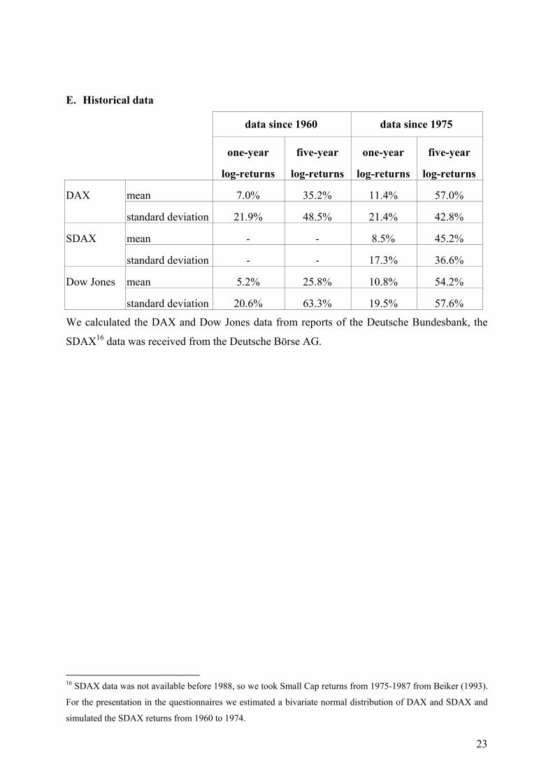
marks we determined the historical average log-returns Mean(hist)j and the historical volatil-

ities (standard deviations) of the log-returns Vol(hist)j by using data since 19606. The table in

appendix E shows the historical benchmarks.

3 Perception of the Expected Returns

Portfolio choice is driven by risk and return. Therefore, we are going to examine the percep-

tion of the expected risk and returns of our three risky asset classes. Turning to returns first7,

the following measure is able to capture significant effects on perceptional biases (participant

i and asset class j =1, 2, 3):

1)hist(Mean

mean)bias(Mean

j

ijij −=

One possible influence on the perception of expected returns might be the individual invest-

ment horizon. Exhibit shows the mean and median biases for all asset classes for the one-year

and five-year investment horizon. Five-year returns tend to be overestimated to a lesser de-

gree than one-year returns: While the one-year DAX-returns tend to be overestimated on av-

erage by 0.93, the five-year DAX-returns tend to be overestimated on average by only 0.50.

The results for the American index Dow Jones are similar. For the small caps index SDAX

we find an underestimation of the one-year returns8, but again the expected return biases for

the five-year investment horizon tend to be below the biases for the one-year returns. Using a

Wilcoxon-test (DAX: p=0.001**, SDAX: p=0.392, Dow Jones: p=0.012*) we find significant

differences between these two investment horizons in this within-subject design.

6 For the small caps we did not get data since 1960, so we estimated the historical benchmarks with data since 1975. 7 Appendix F shows the mean and median values for the five different information conditions and the two se-quence conditions. 8 This is probably due to the different time periods underlying the historical benchmark, however this does not matter since we are interested in the differences between the one-year and five-year investment horizon.

6


We examine sequence effects as we counterbalanced the sequence of the two investment hori-

zons in the questionnaires. Using a Mann-Whitney U test we do not find any significant ef-

fects for all three asset classes and for both investment horizons.

However, we do find significant effects with regard to the type of statistical informa-

tion provided to the participants. Part of the students obtained historical one-year returns

(conditions R- (1) and R+ (1)) the others received historical five-year returns (conditions R-

(5) and R+ (5)). As Exhibit 2 shows, the participants with the long-term information tended to

overestimate the expected returns compared to those participants with the short-term informa-

tion. This holds true for all asset types and for both investment horizons. The one-year DAX-

returns for example tended to be overestimated in the one-year returns condition by an aver-

age of 0.32, whereas in the five-year returns condition they tended to be overestimated by an

average of 1.45. This effect is significant in a between-subject Mann-Whitney U test except

for the five-year SDAX estimates (DAX (one-year): p=0.004**, SDAX (one-year):

p=0.008**, Dow Jones (one-year): p=0.000**, DAX (five-year): p=0.008**, SDAX (five-

year): p=0.083, Dow Jones (five-year): p=0.006**).


4 Volatility Assessments

We now study the perceived standard deviations (volatilities) of the one-year and five-year

log-returns9. Biases in the volatility assessments will be measured relative to our historical

benchmark (participant i and asset class j =1, 2, 3):

1)hist(Vol

int)po(Vol)bias(Vol

j

ijij −=

9 Appendix G shows the average and median volatility forecasts for the five information conditions and the two sequence conditions.

7

We find a significant influence of the individual investment horizon on volatility bias. Assum-

ing a long-term investment horizon our participants tended to underestimate the volatility to a

greater degree than in the short-term setting. While the one-year volatilities had been underes-

timated on average between 0.05 and 0.16, the five-year volatilities were underestimated by

0.26 to 0.50 as (the following) Exhibit 3 shows. These differences are highly significant in a

within-subject Wilcoxon-test (DAX: p=0.000**, SDAX: p=0.002**, Dow Jones: p=0.000**).

This effect is confirmed by a between-subject analysis using only the data in the first envelop.


As in the case of expected returns, we are interested in the informational effects of the pre-

sented one-year versus the five-year returns in conditions R- and R+ as illustrated in (the

next) Exhibit 4. As for the expected returns we find the effect that long-term information

seems to produce higher estimates. Participants provided with the bar charts on the historical

five-year returns they tended to forecast a higher volatility. This is not significant for all esti-

mates in a between-subject Mann-Whitney U test (DAX (one-year): p=0.388, SDAX (one-

year): p=0.945, Dow Jones (one-year): p=0.044*, DAX (five-year): p=0.013*, SDAX (five-

year): p=0.103, Dow Jones (five-year): p=0.001**). The effect seems to be more apparent for

the five-year investment horizon.


5 Subjective Risk Assessments

As an alternative measure of risk we asked our participants to rate the given asset classes on a

scale from 1 to 9 according to the perceived riskiness of the asset. We will analyse the differ-

ences between historical volatility and the subjective risk assessment here, and we will look

for their relevance for subsequent portfolio decisions in section 7.10

10 The average results for all information conditions and the two sequence conditions are illustrated in appendix H.

8

Exhibit 5 summarizes the average subjective risk assessments for the three asset

classes and the two investment horizons. The risk assessments of the five-year investment

horizon tend to be below those of the one-year investment horizon. Comparing the short-term

investment horizon and the long-term investment horizon with a Wilcoxon-test, we again find

significant within-subject differences for all asset classes. (DAX: p=0.000**, SDAX:

p=0.000**, Dow Jones: p=0.000**)


We find significant effects of the sequence in which the investment horizons are presented on

subjective risk assessments. Participants starting with a five-year investment horizon (first

envelope) tend to give higher risk assessments (average over all three assets: 5.46 for one year

vs. 5.13 for five year) than the ones starting with a one-year horizon (average over all three

assets: 5.11 for one year vs. 4.24 for five years). A Mann-Whitney U test finds the between-

subject differences to be significant in the long-term DAX and Dow Jones assessments (DAX

(one-year): p=0.997, SDAX (one-year): p=0.082, Dow Jones (one-year): p=0.103, DAX (five-

year): p=0.001**, SDAX (five-year): p=0.107, Dow Jones (five-year): p=0.011*). Conse-

quently, we find no significant between-subject differences when only regarding the answers

of the first envelope and compare one-year with five-year risk assessments.

This result is in line with psychological results that show that people behave differ-

ently when evaluating decision options either separately or jointly, see Hsee, Loewenstein,

Blount and Bazerman (1999) for a theoretical explanation. In their research they differentiate

between attributes of decision alternatives that are “easy-to-evaluate” and attributes that are

“difficult-to-evaluate”. Their “evaluability hypothesis” states that difficult-to-evaluate attrib-

utes have a larger impact on people’s judgments and choices in a joint evaluation mode than

in a separate evaluation mode. The problems our participants had with the transfer of short-

term volatilities into long-term volatilities suggest that the attribute “investment horizon” is a

difficult-to-evaluate attribute. Hence – according to the evaluability hypothesis – the invest-

ment horizon should affect risk assessments more in a joint than in a separate evaluation

mode. This is exactly what we find. When our participants answered the questions regarding

the second investment horizon they probably compared the two investment horizons. Thus,

9

they judged the risks of the investments in a joint evaluation mode. Consequently, in this

mode the difficult-to-evaluate attribute “investment horizon” had a larger impact on their risk

assessments than in the separate evaluation mode, when they answered the questions of the

first envelope.

Comparing the statistical formats – the historical one-year and five-year returns – we

do not get the same results as for the volatility forecasts. As Exhibit 6 shows, the five-year

returns lead to higher risk assessments only for the Dow Jones but not for the DAX. The

higher risk assessments for the Dow Jones in the five-year conditions R- (5) and R+ (5) are

significant in a Mann-Whitney U test (Dow Jones (one-year): p=0.021*, Dow Jones (five-

year): p=0.004**). The contrasting effects for the DAX are also significant (DAX (one-year):

p=0.002**, DAX (five-year): p=0.019*). We do not find significant differences for the SDAX

(SDAX (one-year): p=0.566, SDAX (five-year): p=0.669).


In summary, we find significant effects of the individual investment horizon on our partici-

pants’ perception of expected returns, volatilities and risk. Their perceptions of the expected

returns relative to a historical benchmark were higher for the one-year scenario than for a

five-year investment horizon. The same holds true and is significant for the forecasted volatil-

ities. We also find this effect to be significant for the given subjective risk assessments but –

in contrast to the estimated expected returns and volatility forecasts – sequence effects play an

important role. In appendix J, we present the correlations between volatility forecasts and risk

assessments for each asset class and for both investment horizons. They tend to be positive

but small (between .2 and .3 for the significant values).

The rational or correct relationship between these long-term and short-term risk as-

sessments depends on the appropriate risk measure and the question whether people rate long-

term and short-term risks on the same scale. While one-year and five-year volatility forecasts

are clearly biased, it is not clear to what extent investors’ risk assessment is irrational. How-

ever the results show that one reason for the comparatively low subjective risk assessments

might be a comparison between a long-term and short-term investment situation.

10

Finally, we examined effects, resulting from differences in the presentation of returns.

About half of the participants were given historical one-year returns while the others got his-

torical five-year returns. For the expected returns and the volatilities, we find significant evi-

dence that presenting five-year returns lead to higher estimations. This is also true for most

risk assessment except for the DAX. For DAX risk assessments we find a significant contrast-

ing effect.11

6 Belief in Mean Reversion

We now investigate if the reduced long-term risk perception might be driven by be-

liefs in mean-reverting returns. For this purpose our questionnaire contained an extra question

about future values of a DM 1,000 investment in the DAX-Fund conditional to a given gain

(of 50%) or a given loss (of 25%) during the first year. 99 data sets could be analyzed, as four

more questionnaires contained incomplete answers to this question. We will denote the one-

year DAX-return from t=0 to t=1 as , the four-year DAX-return from t=1 to t=5

and the five-year DAX-return from t=0 to t=5 . Because of the additivity of the log-

returns we have . With the answers on page 2 and page 3 of the question-

naire – using the method of Pearson and Tukey – we can calculate the unconditional estimates

for the expected value and the standard deviation of and (see also sections 3 and

4). To determine we use the following equation:

10R → 51R →

50R →

R

505110 RRR →→→ =+

( )51RE →

10→ 50R →

( ) ( ) ( )105010511051 RE)R(ERE)RR(ERE →→→→→→ −=−+=

With the additional question, we obtain information about either for the case of a 50%

gain ( ) or for the case of a 25% loss (

51R →

.0ln()5.1ln(R 10 =→ )75R 10 =→ ). Using again the estima-

11 As the historical volatility of the presented five-year returns of the Dow Jones is much higher than the histori-cal volatility of the presented five-year returns of the DAX, although the one-year volatilities are nearly the same, this result is quite understandable. So, most of the participants in the five-year return conditions R- (5) and R+ (5) realized that the Dow Jones had been a riskier investment than the DAX. Consequently, they tended to give different risk assessments for the three asset classes, which leads to the observed effect that the Dow Jones risk assessments are higher and DAX risk assessments are lower in the five-year returns conditions.

11

tion procedure of Pearson and Tukey we calculate conditional expected values and condi-tional standard deviations of R . 51→

RE 1

)( 1RE →

Exhibit 7 shows the unconditional expected returns for the four years from t=1 to t=5

( ) and the conditional expected returns during these years after a gain

( ) and after a loss (

( 51RE →

|RE 51→

)( ))5.1ln(R 10 =→ ( ))75.0ln(R|R 1051E =→→ ) in the first year. Our

participants tended to estimate this expected return significantly higher after a given loss than

after a given gain.


The median of the expected four-year returns after a gain is 28% whereas the median of the

expected four-year returns after a loss is 53%. The same holds for the means: 36% and 56%.

Only 25% of our participants thought that the expected return would be higher after a gain

than after a loss. A within-subject Wilcoxon-test shows that the difference between

and ( ))5.1ln(R|RE 1051 =→→ ( )75.0ln(R| 105 =→→ is highly significant (p=0.000**). The

difference between ( 51→RE and ( ))75.0ln(R|RE 1051 =→→

)5

is also significant (p=0.000**)

but the difference between and ( ))5.1ln(1R|RE 051 =→→ is not (p=0.060). We find

evidence for the belief in mean-reverting returns by most of our participants. The effect seems

to be driven especially by a strong belief in a rising DAX after a loss of 25% during the first

12 months. We will come back to the question, if this behavior could be one explanation of

the underestimation of long-term risks.

)

To derive a more formally based measure for the belief in mean reversion, we examine

the participants’ ideas about the correlation between the DAX-return in the first year and the

DAX-return in the following four years. This measure captures the implicit statistical interre-

lation between the one-year and subsequent four-year expectations.

444444 3444444 21)R,R(Cov

RR511051105110

5110

5110)R(Var)R(Var2)R(Var)R(Var)RR(Var

→→

→→ρ⋅⋅⋅++=+ →→→→→→

12

As we do not know we will assume that the logarithmic returns are normal12.

Therefore we can use the following formula to determine the implicit correlation coefficient

for each participant13:

( 51RVar → )

( ) x)R(Var

)R,R(Cov)R(E

)R(Var)R,R(Cov

)R(ExR|RE10

511010

10

5110511051 ⋅+⋅−==

→

→→→

→

→→→→→

For x=ln(1.5), we will denote the correlation coefficient as rho1 and as var1, for

x=ln(0.75), we will denote the correlation coefficient as rho2 and

( 51RVar → )( )51R →Var as var2. Taking

only those data sets into account, where the results for rho1 and rho2 are between –1 and 1

and the results for var1 and var2 are above zero, 69 (69.7%) of our questionnaires are consis-

tent. The following results will consider only the consistent questionnaires.

As for the conditional expected returns we find strong evidence for the hypothesis that

subjects believe in mean reversion. The calculated rhos are significantly below zero (t-test:

p=0.000** and p=0.000**). The observed distribution is shown in Exhibit 8. rho2 (mean = -

0.4) seems to be lower than rho1 (mean = -0.2). This result is in line with Exhibit 7, which

also shows that the belief in mean reversion is stronger after losses than after gains: People’s

belief in rising stock prices after bad times seems to be more pronounced than their belief in

falling stock prices after good times.


We now investigate, if the rhos help to explain the differences between the perception of

long-term and short-term risks. For this purpose we construct the following ratio:

DAX of assessmentrisk year -oneDAX of assessmentrisk year - fiveratio(DAX)Risk =

We find significant correlations between the risk ratio (DAX) and rho1 (Pearson correlation =

29.4%, p=0.014*; Spearman correlation = 35.8%, p=0.003**) and marginally significant cor-

relations between rho2 and this quotient (Pearson correlation = 22.1%, p=0.068; Spearman

12 Fama (1976) rejects this assumption for daily returns but not for monthly returns. 13 See Green (1993), p73, formula 3-80.

13

correlation = 12.1%, p=0.095). Furthermore, we divide our participants into two groups:

Those who stated a lower DAX risk assessment for the five-year investment horizon (“group

R1”) and those who did not (“group R2”). We find a significantly higher rho1 (Mann-

Whitney U test: p=0.009**) for those students who gave a lower long-term risk assessment

than for those who gave the same or a higher long-term risk assessment. This is not signifi-

cant for rho2. Consequently, it is especially the participants’ belief in negative returns after

rising stock prices that explains the underestimation of long-term risks.

We also examine the relation between the given conditional expected returns and the

risk ratio (DAX). The following ratio is the smaller the stronger the belief in mean-reverting

DAX-returns is:

( )( ))75.0ln(|

)5.1ln(|(DAX)Ration Returns Expected

1051

1051

==

=→→

→→

RRERRE

We do not find a significant Pearson correlation (0.110, p=0.278) between this Expected re-

turns ratio (DAX) and the risk ratio (DAX), however, we do find a marginally significant

Spearman correlation of 19.5% (p=0.054). The difference between the Expected returns ratio

(DAX) is marginally significant when considering consistent questionnaires (Mann-Whitney

U test: p=0.064).

Summarizing, we find evidence for investors’ belief in mean reversion and we think

that this belief helps to explain our participants’ underestimation of long-term risks. The high

rate of consistent answers and the significant correlation between rho1 and the risk ratio

(DAX) between five-year and one-year risk assessments confirm this proposition. The ex-

planatory power of the belief in mean reversion seems to be larger for those participants who

gave consistent conditional expectations for future DAX values.

7 Investment Decisions

Finally, we are interested in portfolio choices and possible explanations for this choice (see

appendix I). We compute the portfolio risk for both the one-year and the five-year investment

14

horizons using the returns, volatilities and correlations estimated with our historical data since

1975 (see appendix E).

∑∑= =

ρ⋅σ⋅σ⋅⋅=−3

1i

3

1jijjiji xxRiskPortfolio

xi denotes the proportion of the three asset types14 (DAX: i=1, SDAX: i=2 and Dow Jones:

i=3), σi the historical standard deviation and ρij the historical correlation between asset i and j

(ρij =1 for i=j). As one would expect, we find high correlations between the total portfolio

risks and the stated risk attitude for both the one-year investment horizon (correlation=0.418,

p=0.000**) and the five-year investment horizon (correlation=0.360, p=0.000**).

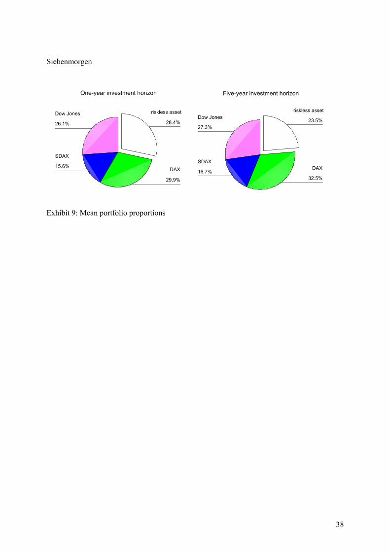
We find significant differences between the one-year and the five-year portfolio risk.

The mean one-year portfolio risk is 13.91% while the average five-year portfolio risk is

14.85%. This difference is significant in a Wilcoxon-test (p=0.011*) and is confirmed by

Exhibit 9, which shows the mean portfolio proportions for the two investment horizons. When

the participants operated in the short-term investment horizon they invested 28.4% in the risk-

less asset. For long-term investment horizon, however, they tended to reduce this proportion

by about 5%.


In a within-subject comparison this tendency is also confirmed: While 51 of our participants

increased the portfolio risk for the long-run portfolio compared to their short-term portfolio,

only 33 participants accepted less portfolio risk for the five-year investment horizon com-

pared to the one-year investment horizon. 9 participants did not change the entire portfolio

risk when deciding for the second investment horizon.

Although we cannot identify a significant influence of the sequence of the investment

horizon on the portfolio risk – probably because of the high variability in our portfolio risk

data – there seems to be some influence of the sequence condition on the portfolio choice. The

14 We find two cases, in which the xi did not add up to 100% (95% and 110%). We divided these xi by the sum of the xi to adjust for these errors.

15

group of participants that began with the questions regarding the five-year investment horizon

shows no tendency to accept more portfolio risk in the long run. 22 of them accepted more

portfolio risk for the five-year horizon, and 21 accepted less risk. In the other condition, how-

ever, 29 of 50 participants increased the risk of the long-term portfolio, after they had first

been confronted with the short-term portfolio. Only 12 of them decreased the portfolio risk in

the long run. Analogously, we find a much larger difference of 1.58% between the long-term

and short-term portfolio risk in the condition, in which participants began with the one-year

investment horizon compared to the small difference of 0.32% in the condition, where the

participants began with the five-year investment horizon. The influence of the sequence con-

dition on the difference between the long-term and short-term portfolio risk is marginally sig-

nificant in a Mann-Whitney U test (p=0.088). This result is in line with our sequence-

dependent risk assessment results presented in section 5. Recall, that the reduction of the risk

assessments in the one-year-five-year condition is larger than the rise of the risk assessments

in the five-year-one-year condition. This implies that it is especially the attribute “long-run

investment horizon” that is difficult-to-evaluate. According to the evaluability hypothesis of

Hsee, Loewenstein, Blount and Bazerman (1999) it would be the evaluation of the five-year

investment horizon in a joint mode, i.e. in the second envelope that drives differences between

the two investment horizons. This is confirmed by the portfolio choice.

As the results of Benartzi and Thaler (1999) suggest, we find that participants receiv-

ing the historical five-year returns tend to accept a higher portfolio risk. But we do not find

that these effects are significant. The reason for this might be that the presentation of five-year

instead of one-year returns has two effects. One the one hand expected returns are perceived

more intensively. On the other hand, however, both volatility and risk15 tend to be overesti-

mated. Thus, it might be the case that these two effects cancel out.

To learn about the effect of different investment horizons on portfolio choice, we fur-

thermore examine which factors drive the observed difference between the one-year and the

five-year portfolio risk (see Exhibit 10). Using the difference between the five-year and the

one-year portfolio risk on the one hand and the difference between the sums of all five-year

15 Regarding the risk assessments we found a contrasting effect for the DAX-returns.

16

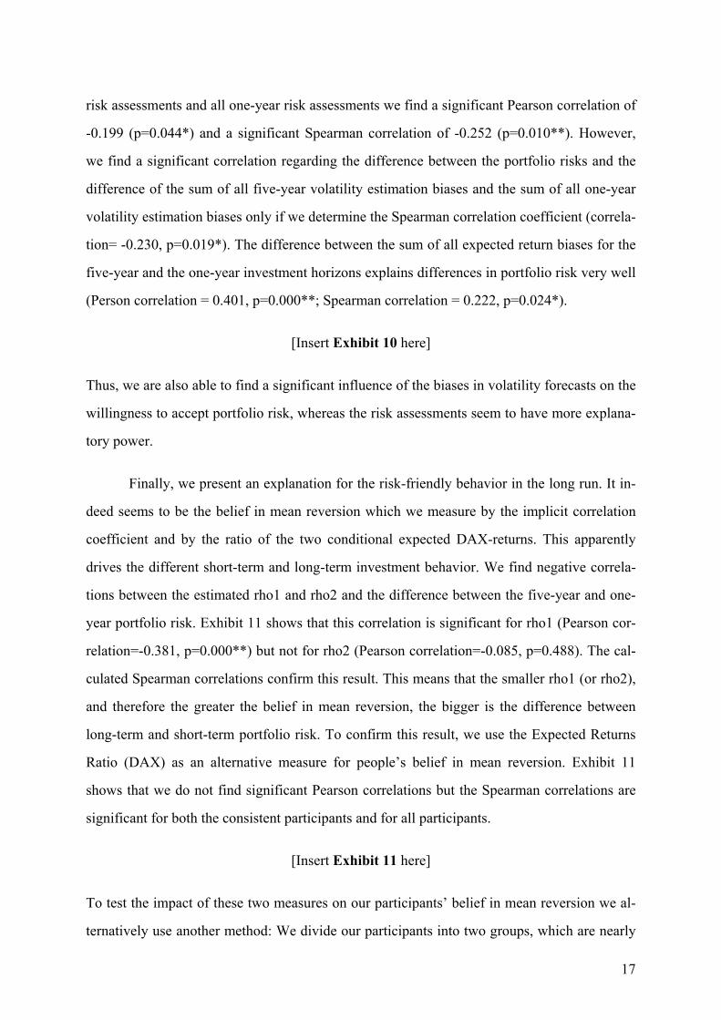
risk assessments and all one-year risk assessments we find a significant Pearson correlation of

-0.199 (p=0.044*) and a significant Spearman correlation of -0.252 (p=0.010**). However,

we find a significant correlation regarding the difference between the portfolio risks and the

difference of the sum of all five-year volatility estimation biases and the sum of all one-year

volatility estimation biases only if we determine the Spearman correlation coefficient (correla-

tion= -0.230, p=0.019*). The difference between the sum of all expected return biases for the

five-year and the one-year investment horizons explains differences in portfolio risk very well

(Person correlation = 0.401, p=0.000**; Spearman correlation = 0.222, p=0.024*).


Thus, we are also able to find a significant influence of the biases in volatility forecasts on the

willingness to accept portfolio risk, whereas the risk assessments seem to have more explana-

tory power.

Finally, we present an explanation for the risk-friendly behavior in the long run. It in-

deed seems to be the belief in mean reversion which we measure by the implicit correlation

coefficient and by the ratio of the two conditional expected DAX-returns. This apparently

drives the different short-term and long-term investment behavior. We find negative correla-

tions between the estimated rho1 and rho2 and the difference between the five-year and one-

year portfolio risk. Exhibit 11 shows that this correlation is significant for rho1 (Pearson cor-

relation=-0.381, p=0.000**) but not for rho2 (Pearson correlation=-0.085, p=0.488). The cal-

culated Spearman correlations confirm this result. This means that the smaller rho1 (or rho2),

and therefore the greater the belief in mean reversion, the bigger is the difference between

long-term and short-term portfolio risk. To confirm this result, we use the Expected Returns

Ratio (DAX) as an alternative measure for people’s belief in mean reversion. Exhibit 11

shows that we do not find significant Pearson correlations but the Spearman correlations are

significant for both the consistent participants and for all participants.


To test the impact of these two measures on our participants’ belief in mean reversion we al-

ternatively use another method: We divide our participants into two groups, which are nearly

17

equal in size. The participants that increase their long-term portfolio risk compared to their

short-term portfolio risk are denoted as “group P1”; all other participants are denoted as

“group P2”. Exhibit 11 shows the mean values for rho1, rho2 and the Expected Value Quo-

tient (DAX) for both groups P1 and P2. All measures tend to be smaller for group P1. We use

a Mann-Whitney U test to examine whether the difference between the two groups is signifi-

cant. Our results show that rho1 of group P1 is significantly smaller than rho1 of group P2

(p=0.003**), which confirms that those investors which increase their portfolio risk in the

long run (group P1) show a stronger belief in mean reversion. This is again not significant for

rho2 (p=0.118). Regarding the Expected Returns Ratio (DAX) we find a significant difference

between the two groups only among the consistent participants (p=0.038*), however, for all

participants the effect is still marginally significant (p=0.084).

8 Conclusion

With this study we intend to examine the effect of different investment horizons on risk per-

ception, expected returns and portfolio choice. We find that there are significant differences

between short-term and long-term risk perception. Both the estimated volatilities and the sub-

jective risk assessments depend on the given investment horizon. We find that biases in risk

assessments rather than biases in estimated volatilities drive the observed investment behav-

ior. Consequently, we also detect significant differences in the short-term and long-term total

portfolio risk that participants are willing to take. One reason for this seems to be the belief in

mean-reverting asset prices. Most of our participants believe in this, although empirical re-

sults indicate that the subsequent four-year return is positively correlated with the return in the

first year (see Bromann et al., 1997 or Schiereck, et al., 1999 and DeBondt and Thaler, 1989

for a survey). Nevertheless the observed belief in mean reversion seems to drive the risk-

taking behavior in the long run. Furthermore, we cannot reject limited cognitive abilities as

another reason for this specific horizon-dependent risk behavior.

18

Appendix

A. Questionnaire (page 1, annual returns)

Investment Questionnaire

Please imagine, you will inherit DM 500,000 in the next days. But you must not consume this money; you have to decide today, how to invest it. The following investment alternatives are available:

„riskless investment“ investment without price risk and with sure payments with a annual rate of return of 5%

„DAX-Fund“ portfolio of 30 German Blue Chips, as they are in the German Stock Index DAX

„SDAX-Fund“ portfolio of smaller German stocks, whose market capitalization is ranked 101 to 200, as they are in the German Small Cap Index SDAX

„Dow Jones-Fund“ portfolio of 30 U.S. Bluechips, as they are in the index Dow Jones

-50%

-25%

0%

25%

50%

75%

1960

1965

1970

1975

1980

1985

1990

1995

Ann

ual D

ow J

ones

-ret

urns

(in D

M)

-50%

-25%

0%

25%

50%

75%

1960

1965

1970

1975

1980

1985

1990

1995

Ann

ual S

mal

l Cap

-re

turn

s

-50%

-25%

0%

25%

50%

75%

1960

1965

1970

1975

1980

1985

1990

1995

Ann

ual D

AX

-ret

urns

19

B. Questionnaire (page 1, 5-year returns)

Investment Questionnaire

Please imagine, you will inherit DM 500,000 in the next days. But you must not consume this money; you have to decide today, how to invest it. The following investment alternatives are available:

„riskless investment“ investment without price risk and with sure payments with a annual rate of return of 5%

„DAX-Fund“ portfolio of 30 German Blue Chips, as they are in the German Stock Index DAX

„SDAX-Fund“ portfolio of smaller German stocks, whose market capitalization is ranked 101 to 200, as they are in the German Small Cap Index SDAX

„Dow Jones-Fund“ portfolio of 30 U.S. Bluechips, as they are in the index Dow Jones

-100%-50%

0%50%

100%150%200%250%300%

60-64 65-69 70-74 75-79 80-84 85-89 90-94 95-99

5-ye

ar D

ow J

ones

-ret

urns

(in D

M)

-100%-50%

0%50%

100%150%200%250%300%

60-64 65-69 70-74 75-79 80-84 85-89 90-94 95-99

5-ye

ar S

mal

l Cap

-ret

urns

-100%-50%

0%50%

100%150%200%250%300%

60-64 65-69 70-74 75-79 80-84 85-89 90-94 95-995-ye

ar D

AX

-ret

urns

20

C. Questionnaire (page 2/3) Please imagine, you would like to invest your money for 12 months. So your investment horizon is 1 year.

How do you assess future values of the mentioned investment alternatives in the next 12 months? Please consider all gains/losses, dividend payments and if necessary exchange rate risks.

If you invest today DM 1,000 into the mentioned investments, what are these DM 1,000 worth in one year? Please state the amount of money (in DM), of which you think the real value in 12 months will, ...

lower bound: ... rather not (i.e. in only 10% of all cases) remain under it. median: ... equally likely exeed it or remain under it. upper bound: ... rather not (i.e. in only 10% of all cases) exeed it.

1000 DM will be... in DAX-Fund in SDAX-Fund in Dow Jones-Fund

lower bound

median

upper bound

How do you assess the risk of these three investments on a scale from 1 to 9 ? (1= no risk; 5=moderate risk; 9=highest risk) DAX-Fund SDAX-Fund Dow Jones-Fund

risk assessment

How do you allocate your new wealth of DM 500,000 for the next 12 months using the available investment alternatives, if you are not allowed to change your portfolio allocation during the next 12 months? Please insert percentages.

Riskless investment with a return of 5%

DAX-Fund

SDAX-Fund

Dow Jones-Fund

Sum

Please make sure, that your portfolio portions add up to 100%.

DM DM DM

DM DM DM

DM DM DM

%

%

%

%

100%

21

D. Questionnaire (page 4) Extra question:

Please imagine, after one year an investment of DM 1,000 into the DAX-Fund has reached an value of DM 1,500. So the DAX-Fund has won 50% after 12 months. What do you think in such a situation, what is this investment worth after 4 more years (5 years altogether)? Please estimate again the lower bound, the median and the upper bound of the final value. After 5 years DM 1,000 invested in the DAX-Fund will be worth, ...

... if DAX-Fund has won 50% after the first year.

lower bound

median

upper bound

And what about a DM 1,000 investment into the DAX-Fund after 5 years, if it is worth only DM 750 after the 12 months?

After 5 years DM 1,000 invested in the DAX-Fund will be worth, ...

... if DAX-Fund has lost 25% after the first year.

lower bound

median

upper bound

Finally two personal questions:

Are you male or female ?

How would you assess your risk attitude in such a situation, in which you have to invest DM 500,000 DM? Please mark the scale.

conservative moderate aggressive

Thank your very much for your help.

0

500

1000

1500

2000

2500

3000

0 1 2 3 4 5

years

valu

e D

ax-F

und

(in D

M)

?750

0

500

1000

1500

2000

2500

3000

0 1 2 3 4 5

years

valu

e D

ax-F

und

(in D

M)

?1500

DM

DM

DM

DM

DM

DM

22

E. Historical data

data since 1960 data since 1975

one-year

log-returns

five-year

log-returns

one-year

log-returns

five-year

log-returns

mean 7.0% 35.2% 11.4% 57.0% DAX

standard deviation 21.9% 48.5% 21.4% 42.8%

mean - - 8.5% 45.2% SDAX

standard deviation - - 17.3% 36.6%

mean 5.2% 25.8% 10.8% 54.2% Dow Jones

standard deviation 20.6% 63.3% 19.5% 57.6%

We calculated the DAX and Dow Jones data from reports of the Deutsche Bundesbank, the

SDAX16 data was received from the Deutsche Börse AG.

16 SDAX data was not available before 1988, so we took Small Cap returns from 1975-1987 from Beiker (1993).

For the presentation in the questionnaires we estimated a bivariate normal distribution of DAX and SDAX and

simulated the SDAX returns from 1960 to 1974.

23

F. Estimation of expected returns

One-year investment horizon:

.15 .15 .07 .06 .24 .14 .06 .06 .14 .15

.11 .11 .06 .05 .12 .05 .04 .03 .10 .11

.18 .14 .06 .05 .23 .16 .06 .06 .13 .19

.14 .14 .14 .15 .14 .13 .10 .09 .18 .17

.09 .10 .07 .05 .13 .09 .05 .05 .08 .07

.10 .09 .11 .11 .19 .15 .07 .09 .21 .21

DAXSDAXDow Jones

page 2

DAXSDAXDow Jones

page 3

one-yearinvestmenthorizon

Mean MedianN

Mean MedianR- (1)

Mean MedianR- (5)

Mean MedianR+ (1)

Mean MedianR+ (5)

information conditions

Five-year investment horizon:

.47 .42 .50 .23 .67 .54 .51 .46 .64 .61

.38 .34 .44 .25 .44 .28 .44 .38 .53 .56

.52 .34 .51 .20 .62 .64 .53 .47 .62 .61

.55 .51 .51 .53 .74 .61 .28 .26 .48 .53

.50 .36 .37 .24 .57 .40 .23 .22 .27 .26

.52 .51 .47 .36 .71 .66 .27 .26 .54 .52

DAXSDAXDow Jones

page 3

DAXSDAXDow Jones

page 2

five-yearinvestmenthorizon

Mean MedianN

Mean MedianR- (1)

Mean MedianR- (5)

Mean MedianR+ (1)

Mean MedianR+ (5)


G. Volatility forecasts


.15 .18 .20 .21 .26 .20 .15 .15 .22 .19

.21 .19 .14 .14 .19 .14 .12 .12 .19 .18

.14 .14 .21 .22 .33 .25 .14 .15 .21 .18

.21 .25 .19 .18 .18 .18 .13 .07 .17 .10

.22 .16 .17 .16 .10 .10 .11 .05 .14 .07

.20 .19 .16 .17 .21 .20 .15 .12 .23 .14

DAXSDAXDow Jones

page 2

DAXSDAXDow Jones

page 3


Mean MedianN

Mean MedianR- (1)

Mean MedianR- (5)

Mean MedianR+ (1)

Mean MedianR+ (5)



.24 .23 .25 .22 .49 .43 .22 .22 .32 .28

.30 .32 .22 .19 .35 .18 .19 .21 .35 .33

.25 .26 .26 .21 .57 .56 .20 .22 .37 .38

.24 .21 .45 .35 .33 .36 .15 .14 .26 .27

.31 .22 .41 .25 .26 .27 .14 .13 .19 .13

.26 .23 .40 .29 .41 .47 .17 .13 .32 .26

DAXSDAXDow Jones

page 3

DAXSDAXDow Jones

page 2


Mean MedianN

Mean MedianR- (1)

Mean MedianR- (5)

Mean MedianR+ (1)

Mean MedianR+ (5)


24

H. Subjective Risk Assessments


3.90 5.71 4.33 5.50 4.506.40 4.57 4.44 4.75 5.254.00 5.43 6.89 5.42 5.675.18 5.50 3.89 4.55 4.336.27 6.50 4.67 5.18 5.676.00 4.90 6.67 6.18 6.33

DAXSDAXDow Jones

page 2

DAXSDAXDow Jones

page 3


MeanN

MeanR- (1)

MeanR- (5)

MeanR+ (1)

MeanR+ (5)



2.70 4.71 3.78 3.42 3.755.30 4.29 4.22 3.67 4.673.10 5.29 6.44 3.58 5.504.36 5.80 3.89 4.82 4.085.73 5.50 4.11 4.45 5.255.18 5.20 7.22 5.64 5.83

DAXSDAXDow Jones

page 3

DAXSDAXDow Jones

page 2


MeanN

MeanR- (1)

MeanR- (5)

MeanR+ (1)

MeanR+ (5)


I. Portfolio Proportions


.24 .23 .36 .40 .30 .25 .25 .23 .35 .23

.31 .30 .16 .20 .32 .33 .30 .28 .26 .30

.14 .15 .21 .20 .18 .20 .15 .10 .15 .20

.31 .25 .27 .25 .21 .20 .30 .28 .23 .28

.24 .20 .35 .28 .28 .25 .27 .30 .23 .20

.34 .30 .28 .25 .31 .30 .37 .40 .30 .30

.18 .15 .09 .05 .21 .20 .16 .11 .12 .10

.24 .30 .29 .28 .19 .15 .20 .15 .35 .30

risklessDAXSDAXDow Jones

page 2


page 3


Mean MedianN

Mean MedianR- (1)

Mean MedianR- (5)

Mean MedianR+ (1)

Mean MedianR+ (5)



.23 .20 .26 .20 .32 .20 .20 .10 .14 .14

.31 .35 .25 .25 .30 .33 .33 .35 .42 .38

.17 .15 .19 .20 .19 .17 .15 .13 .18 .20

.29 .30 .31 .30 .20 .20 .32 .40 .26 .30

.24 .25 .35 .30 .27 .25 .21 .20 .20 .13

.32 .30 .22 .23 .38 .35 .36 .30 .32 .30

.20 .20 .12 .13 .19 .15 .18 .20 .13 .13

.24 .25 .32 .30 .15 .10 .26 .25 .35 .30


page 3


page 3


Mean MedianN

Mean MedianR- (1)

Mean MedianR- (5)

Mean MedianR+ (1)

Mean MedianR+ (5)


25

J. Correlations between volatility forecasts and risk assessments

Investment Horizon Correlation (Pearson) Correlation (Spearman)

DAX one-year 0.218 (p=0.027*) 0.205 (p=0.038*)

SDAX one-year 0.284 (p=0.004**) 0.304 (p=0.002**)

Dow Jones one-year 0.173 (p=0.081) 0.065 (p=0.516)

DAX five-year 0.107 (p=0.281) 0.081 (p=0.416)

SDAX five-year 0.140 (p=0.159) 0.090 (p=0.364)

Dow Jones five-year 0.222 (p=0.024*) 0.216 (p=0.029*)

26

References

Anderson, B.F./Settle, J.W. (1996): The Influence of Portfolio Characteristics and Invest-ment Period on Investment Choice. Journal of Economic Psychology, 17, 343-358.

Beiker, H. (1993): Überrenditen und Risiken kleiner Aktiengesellschaften: eine theoretische und empirische Analyse des deutschen Kapitalmarkts von 1966 bis 1989. Müller Bo-termann, Köln.

Benartzi, S./Thaler, R.H. (1999): Risk Aversion or Myopia? Choices in Repeated Gambles and Retirement Investments. Management Science, 45, 364-381.

Bromann, O./Schiereck, D./Weber, M. (1997): Reichtum durch (anti-)zyklische Handels-strategien am deutschen Aktienmarkt? Schmalenbachs Zeitschrift für betriebswirtschaft-liche Forschung, 49, 603-616.

Clotfelder, C.T./Cook, P.J. (1993): The ‘Gambler’s Fallacy’ in Lottery Play. Management Science, 39, 1521-1525.

DeBondt, W.F.M./Thaler, R.H. (1989): Anomalies – A Mean-Reverting Walk Down Wall Street. Journal of Economic Perspectives, 3, 189-202.

Fama, E.F. (1976): Foundations of Finance. Basic Books, New York.

Green, W.H. (1993): Econometric Analysis (2nd edition). Macmillan Publishing Company, New York.

Hsee, C.K./Loewenstein, G.F./Blount, S./Bazerman, M.H. (1999): Preference Reversals between Joint and Separate Evaluations of Options: A Review and Theoretical Analy-sis. Psychological Bulletin, 125, 576-590.

Keefer, D.L./Bodily, S.E. (1983): Three-point Approximation for Continuous Random Vari-ables. Management Science, 29, 595-609.

Klos, A./Langer,T./Weber, M. (2002): Über kurz oder lang: welche Rolle spielt der Anlage-horizont bei der Bwertung von Investments?, Working Paper, University of Mannheim.

Kritzman, M. (1994): What Practitioners Need to Know about Time Diversification. Finan-cial Analysts Journal, 50, 14-18.

27

Langer, T./Weber, M. (2001): Prospect Theory, Mental Accounting, and Differences in Ag-gregated and Segregated Evaluation of Lottery Portfolios. Management Science, 47, 716-733.

Odean, T. (1998): Are Investors Reluctant to Realize Their Losses? The Journal of Finance, 53, 1775-1798.

Schiereck, D./DeBondt, W./Weber, M. (1999): Contrarian and Momentum Strategies in Germany. Financial Analysts Journal, 55, 104-116.

Schooley, D.K./Worden, D.D. (1999): Investors’ Asset Allocation versus Life-Cycle Funds. Financial Analysts Journal, 55, 37-43.

Shefrin, H./Statman, M. (1985): The Disposition to Sell Winners Too Early and Ride Losers Too Long: Theory and Evidence. The Journal of Finance, 40, 777-792.

Siebenmorgen, N./Weber, E.U./Weber, M. (2001): Communicating Asset Risk: How the format of historic volatility information affects risk perception and investment deci-sions. Working Paper 00-38, Sonderforschungsbereich 504, Universität Mannheim.

Terrell, D. (1998): Biases in Assessments of Probabilities: New Evidence from Greyhound Races. Journal of Risk and Uncertainty, 17, 151-166.

28

Siebenmorgen

belief

in mean

reversion

not significant

only for differences between one-year and five-year in-vestment horizons

not for DAX

total

risk of

portfolio sequence

one-year horizon first or

five-year horizon first

presented returns

1-year or five-year re-

selection

of asset

classes

subjective

perception

of expected

returns

subjective

risk per-

ception

subjective

volatility

forecasts

presentation format

N, R- or R+

investment horizon

1 year or 5 years

Exhibit 0: Influence of different conditions on risk perception and investment decisions

29

Siebenmorgen

.93 .82-.03 -.151.59 1.09.50 .39

-.09 -.251.04 .69

DAXSDAXDow Jones


DAXSDAXDow Jones


biasMean Median

Exhibit 1: Biases in estimated returns for different investment horizons

30

Siebenmorgen

.32 .19 1.45 1.02-.39 -.45 .21 .04.49 .73 2.63 2.47.26 .09 .76 .61

-.19 -.37 -.02 -.18.70 .37 1.39 1.35

DAXSDAXDow Jones


DAXSDAXDow Jones


biasMean Medianone-year returns

Mean Medianfive-year returns

statistical information

Exhibit 2: Biases in estimated returns in different statistical settings

31

Siebenmorgen

-.16 -.22-.08 -.26-.05 -.13-.40 -.47-.26 -.38-.50 -.59

DAXSDAXDow Jones


DAXSDAXDow Jones


biasMean Median

Exhibit 3: Biases in volatility forecasts for different investment horizons

32

Siebenmorgen

-.26 -.27 -.07 -.19-.23 -.27 -.09 -.37-.22 -.27 .17 -.03-.46 -.55 -.30 -.40-.36 -.49 -.22 -.28-.60 -.65 -.36 -.41

DAXSDAXDow Jones


DAXSDAXDow Jones


biasMean Medianone-year returns

Mean Medianfive-year returns


Exhibit 4: Biases in volatility forecasts in different statistical settings

33

Siebenmorgen

4.735.415.754.114.745.25

DAXSDAXDow Jones


DAXSDAXDow Jones


Riskassessment

Mean

Exhibit 5: Subjective risk assessments for different investment horizons

34

Siebenmorgen

5.28 4.295.28 5.075.50 6.334.63 3.884.45 4.624.85 6.17

DAXSDAXDow Jones


DAXSDAXDow Jones


Riskassessment

Mean

one-yearreturns

Mean

five-yearreturns


Exhibit 6: Subjective risk assessments in different statistical settings

35

Siebenmorgen

Mean Median

( )51RE → 39.3 % 35.1 %

( )5.1ln(R|RE 1051 =→→ ) 36.3 % 28.2 %

( )75.0ln(R|RE 1051 =→→ ) 55.6% 53.0 %

Exhibit 7: Unconditional and conditional expected DAX-returns

36

Siebenmorgen

rho1

1.0.8.6.4.2-.0-.2-.4-.6-.8-1.0

num

ber o

f obs

erva

tions

16

14

12

10

8

6

4

2

0

Std. Dev = .27 Mean = -.2

N = 69.00

rho2

1.0.8.6.4.2-.0-.2-.4-.6-.8-1.0

num

ber o

f obs

erva

tions

10

8

6

4

2

0

Std. Dev = .41 Mean = -.4

N = 69.00

Exhibit 8: Histograms of rho1 and rho2

37

Siebenmorgen

One-year investment horizon

26.1%

15.6%

29.9%

28.4%

Dow Jones

SDAX

DAX

riskless asset

Five-year investment horizon

27.3%

16.7%32.5%

23.5%Dow Jones

SDAXDAX

riskless asset

Exhibit 9: Mean portfolio proportions

38

Siebenmorgen

Correlation between the difference between

five-year and one-year portfolio risk and …

… the difference of

5-year and 1-year

biases in perceived

expected returns

… the difference

of 5-year and

1-year biases in

volatility forecasts

… the difference of

five-year and one-

year total subjective

risk assessments

Pearson correlation +0.401 (p=0.000**) -0.121 (p=0.223) -0.199 (p=0.044*)

Spearman correlation +0.222 (p=0.024*) -0.230 (p=0.019*) -0.252 (p=0.010**)

Exhibit 10: Correlation between differences of portfolio risk and total perceptions

39

Siebenmorgen

rho1 rho2

Expected Returns Ratio

(DAX)

N=69 N=69 N=69 N=99

Pearson correlation with

difference of long-term and

short-term portfolio risk

-0.381

(p=0.001**)

-0.085

(p=0.488)

-0.009

(p=0.947)

-0.098

(p=0.334)

Spearman correlation with

difference of long-term and

short-term portfolio risk

-0.359

(p=0.002**)

-0.156

(p=0.201)

-0.240

(p=0.047*)

-0.211

(p=0.036*)

Mean for group P1 -0.31 -0.48 0.30 0.19

Mean for group P2 -0.12 -0.30 0.84 0.79

Significance of difference

between P1 and P2

(Mann-Whitney U test)

p=0.003** p=0.118 p=0.038* p=0.084

Exhibit 11: Correlation between differences of portfolio risk and belief in mean reversion

40

The Influence of Different Investment Horizons on Risk · Niklas Siebenmorgen* / Martin Weber∗...

Documents

Transcript of The Influence of Different Investment Horizons on Risk · Niklas Siebenmorgen* / Martin Weber∗...