The Influence of a Steel Casing on the Axial Capacity of a ... · axial capacity of drilled shafts...

TECHNICAL REPORT STANDARD TITLE PAGE

2. Govern""nt Accession No. 3. Recip,ent's Catalog No. f

F~/TX-82/2U255-~~~~~~~~~~~~~~~~~~~~~~~~~~.J

1. Report No.

4. T,tle and Subtille 5. Report Dote

THE INFLUENCE OF A STEEL CASING ON THE AXIAL CAPACITY OF A DRILLED SHAFT

7. Author' 51

Mark J. Owens and Lymon C. Reese

9. Performing Organization Nome and Address

Center for Transportation Research

July 1982 6. Performing Organi Iatian Code

8. Performing OrganiIalian Report No.

Research Report 255-1F

10. Work Unit No.

11. Contract or Grant No. The University of Texas at Austin Research Study 3-5-80-255 Austin, Texas 78712-1075

---.~----------~----~~-------------------------------~ 12. Spon.oring Agency Name and Addrus

Texas State Department of Highways and Public Transportation; Transportation Planning Division

Po O. Box 5051 Austin, Texas 78763

r---1.'5 Supplementary Note.

13. Type of Report and Period Covered

Final

14. Span.oring Agency Code

S1:~dy conducted in cooperation with the U. S. Department of Transportation, Federal Highway Administration. Research Study Title: "The Influence of Steel Casing on the Load Carrying Capaci ty of Dri lled Shafts II

~6-.·~A~b-.~tr~oc~t~~~~=-~~~~~~~~~~~~~~~~~~~------------------------------------1

A series of field load tests were performed to investigate the effects on the axial capacity of drilled shafts when casings could not be pulled. The tests show that leaving casing in place is detrimental, but grouting proved an effective remedial measure when the casing was placed in an oversized excavation. Even though grouting was found to improve the capacity of a shaft where casing was left in place, procedures should be used in the field that will insure that casing will be removed. Shafts cast in the normal manner perform better than do shafts where casing has been grouted. Useful data were obtained on the distribution of axial load from drilled shafts to the supporting soil.

17. Key Warda

drilled shaft, axial capacity, steel casing, load test, grouting, vibrating hammer, over-sized excavation

18. Dialribulion S'.'ement

No restrictions. This document is available to the public through the National Technical Information Service, Springfield, Virginia 22161.

19. Security Ciani'. (of thl. r.p.rt)

Unclassified

20. Security Clollif. (of thit pooel 21. No. of Page. 22. Price

Unclassified 228

Form DOT F 1700.7 (8-691

THE INFLUENCE OF A STEEL CASING ON THE AXIAL CAPACITY

OF A DRILLED SHAFT

by

Mark J. Owens Lymon C. Reese

Research Report Number 255-1F

The Influence of Steel Casing on the Load Carrying Capacity of a Drilled Shaft

Research Study 3-5-80-255

conducted for

Texas

State Department of Highways and Public Transportation

in cooperation with the U. S. Departmellt uf Transportation

Federal Highway Administration

by

CENTER FOR TRANSPORTATION RESEARCH

THE UNIVERSITY OF TEXAS AT AUSTIN

July 1982

The contents of this report reflect the views of the authors, who are responsible for the facts and the accuracy of the data presented herein. The contents do not necessarily reflect the official views or policies of the Federal Highway Administration. This report does not constitute a standard, specification, or regulation.

There was no invention or discovery conceived or first actually reduced to practice in the course of or under this contract, including any art, method, process, machine, manufacture, design or composition of matter, or any new and useful improvement thereof, or any variety of plant which is or may be patentable under the patent laws of the United States of America or any foreign country.

ii

PREFACE

This report presents the results of field studies of the behavior of

drilled shafts under axial load with special reference to the case where

casing could not be pulled.

The authors wish to thank the State Department of Highways and Public

Transportation for their sponsorship of the work and to express appreciation

for the assistance given by many members of their staff. Partial sponsorship

of the System of The University of Texas of the tests at Site 1 in Galveston

is acknowledged and appreciation is expressed to the staff of Facilities

Planning and Construction for their interest and assistance. Appreciation is

also expressed to Walter P. Moore and Associates, Inc.; Louis Lloyd Oliver,

Architect; and McBride-Ratliff and Associates for their interest and assistance

in the Galveston project.

Appreciation is expressed to Farmer Foundation Company who made a

financial contribution to the work in Galveston and carried out the construction

work in a careful and expeditious manner.

July 1982

iii

Mark J. Owens

Lymon C. Reese

ABSTRACT

A series of field load tests were performed to investigate the effects

on the axial capacity of drilled shafts when casings could not be pulled.

The tests show that leaving casing in place is detrimental, but grouting

proved an effective remedial measure when the casing was placed in an over

sized excavation. Even though grouting was found to improve the capacity of

a shaft where casing was left in place, procedures should be used in the

field that will insure that casing will be removed. Shafts cast in the

normal manner perform better than do shafts where casing has been grouted.

Useful data were obtained on the distribution of axial load from drilled

shafts to the supporting soil.

v

SUMMARY

The studies reported herein were concerned with evaluating the effects

on the axial capacity of drilled shafts when casing could not be pulled and

had to be left in place. Two cases were investigated, when casing was placed

in an over-sized excavation and when the casing was driven with a vibratory

hammeL In both instances, it was learned that the failure to extract the

casing had a detrimental effect on the load-carrying capacity of the drilled

shaft.

Grouting was found to be an effective method of restoring he capacity

of two drilled shafts in this test program when the casing was placed in an

over-sized excavation. Even though grouting was found to improve the capacity

of a shaft where casing was left in place, procedures should be used in the

field that will insure that casing will be removed. Shafts cast in the normal

manner perform better than do shafts where casing has been grouted.

A method was suggested for verifying the integrity of drilled shafts when

such a remedial measure is employed. Data were obtained and evaluated on the

distribution of axial load in skin friction and end bearing. The results

from the analysis of these data will prove useful to designers.

vii

IMPLEMENTATION STATEMENT

The information presented in this report is recommended for consideration

by the Bridge Division of the State Department of Highways and Public Trans

portation. The results of the research on the behavior of drilled shafts when

casing is left in place provides positive information to allow the engineering

staff of SDHPT to take appropriate action when the occasion arises. Data that

were acquired on the behavior of instrumented drilled shafts under axial load

will provide additional information related to procedures for design. This

new information, along with similar data acquired in the past, will provide

useful guidance to the designer.

Even though grouting was found to improve the capacity of a shaft where

casing was left in place, procedures should be used in the field that will

insure that casing will be removed. Shafts cast in the normal manner perform

better than do shafts where casing has been grouted.

ix

TABLE OF CONTENTS

PREFACE •• · . . . ABSTRACT . . . . SUMMARY •

IMPLEMEI.~TATION STATEMENT . . . . . CHAPTER 1. INTRODUCTION . . . . . . . ... . . . . . . . . . . . . . . CHAPTER 2. SITE CONDITIONS . . .

Site 1 ~ Galveston, Texas Site Location Soil Profile •••••

Site 2 - Galveston, Texas •••• Site Location Soil Profile ••••••••••

Site 3 - Eastern Site

· . . .

Site Location •••• Soil Profile • •

. . . .

CHAPTER 3. INSTRUMENTATION • • • . . . . . . . Measurement of Axial Load at the Top of the Shaft Measurement of Movements at the Top of the Shaft Measurement of Loads at Selected Locations within Testing of Mustran Cells . • • . Readout System • • • • • • • • • • . • . . . ••

CHAPTER 4. SHAFT INSTALLATION AND CONSTRUCTION PROCEDURES

Test Site 1 - Galveston, Texas Test Shafts • • • • • Grouting of Test Shafts Reaction Shafts ••••

Test Site 2 - Galveston, Texas Test Shaft • • •

. . . .. .

. . . Reaction Shafts . . . . . . . . . . . . .

.xi

. . .

· . . . the Shaft

· . . .

· . . .

Page

iii

v

vii

ix

1

7

7 7 7

15 15 15

19 19 19

23

23 26 26 33 36

39

39 39 44 45

47 47 48

xii

Test Site 3 - Eastern Site Test Shafts . . Reaction Shafts . . .

CHAPTER 5. LOAD TESTS

Test Procedure Test Site I - Galveston, Texas

Test Arrangement . .

Test

Test Results . . . .

Site Test Test

Test Shaft G-I Test Shaft G-2 Test Shaft G-3

2 - Galveston, Arrangement . Results .

Texas

Test Site 3 - Eastern Site Test Arr angemen t Test Results .

Test Shaft E-I Test Shaft E-2

CHAPTER 6. ANALYSIS AND DISCUSSION OF LOAD TESTS

Method of Analysis . . . . . . Mustran Cell Behavior . . Calibration of Mustran Cells Load Distribution Curves Tip Load . . . . . . . . . Side Resistance Shaft Movement

Analysis of Load Tests Test Shaft G-I Test Shaft G-3, Test I Test Shaft G-3, Test 2 Test Shaft G-4 Test Shaft E-I Test Shaft E-2

Page

. . . . 4B 48 51

53

53 54 54 54 54 56 58

60 60 60

. . . . 64 64 64 64 67

71

71 71 71 73 73 75 76

78 78 82 82 82 90 90

Discussion of Load Tests . . Tip Resistance in Clay Tip Resistance in Sand Side Resistance in Sand Side Resistance in Clay .

Influence of Construction Methods

CHAPTER 7. SUGGESTIONS CONCERNING MODIFICATIONS

xiii

Page 97 97

· 102 · . 104 · . 114

• • 119

OF CONSTRUCTION SPECIFICATIONS . • . . . . . . . . . . . . 129

CHAPTER 8. CONCLUSIONS AND RECOMMENDATIONS

Conclusions Recommendations

APPENDIX A. LOGS OF BORINGS . . APPENDIX B. PREPARATION AND INSTALLATION OF MUSTRAN CELLS •

APPENDIX C. TYPES OF INTERNAL INSTRUMENTATION FOR USE IN DRILLED SHAFTS FOR MEASUREMENT OF AXIAL LOAD

· • 133

• 133 · 134

• • , • 139

· 169

AS A FUNCTION OF DEPTH • • • • • • • • • • • • • • • 195

APPEND IX D. CONS TRUCTION S I TUA TrONS WHERE CAS ING WOUIlJ BE D IFF ICULT TO REMOVE . • • • • • • • • • 201

REFERENCES . • • 203

Table

6.1

LIST OF TABLES

Tabulation of theoretical values of bearing capacity in sand . . .

6.2 Tabulation of theoretical values for skin

6.3

6.4

6.5

6.6

friction of drilled shafts in sand . .

Tabulation of theoretical values for skin friction of drilled shafts in sand . .

Comparison of measured and theoretical values of K and x for test site 1 . . . . . . . .

Comparison of measured and theoretical values of K and x for test site 3 . . . . . . . .

Comparison of measured and theoretical values of a

6.7 Tabulation of theoretical values for skin friction of driven piles in sand . . .

xv

Page

103

105

109

112

113

118

124

Figure

1.1

1.1

2.1

2.2

2.3

2.4

2.5

2.6

2.7

2.8

2.9

2.10

3.1

3.2

3.3

3.4

3.5

3.6

3.7

LIST OF FIGURES

Casing method of construction . . . . .

(Cont'd) Casing method of construction

Location of test site 1 and test site 2

Test site 1, soil boring locations

Soil profile, test site 1

Penetration resistance as a function of depth for test site 1 . . . . •

Undrained shear strength as a function of depth test site 1

Soil boring locations, test site 2

Soil profile, teEt site 2 .

Penetration resistance and undrained shear strength as a function of depth, test site 2 .. . . . .

Soil profile, test site 3

Penetration resistance as a function of depth, test site 3 . . . . . .

Schematic of loading system arrangement

Photographs of instrumentation at top of shaft

Components of mustran cell

Schematic arrangement of mustran cell pressurization system . . . . . .

Photographs of isntalled mustran cells

Relative positions of soil layers and mustran cells

Terminal strips and connectors in manifold

xvii

Page

2

3

8

9

10

13

14

16

17

18

20

21

... 24

25

28

29

31

32

34

xviii

Figure Page

3.8 Mustran cell in triaxial type set up . . 35

3.9 Collapsed radiator hose on mustran cell 35

3.10 Vishay automatic data logging system 37

3.11 Portable strain indicator and switch and balance units 37

4.1 Method of construction of test shaft G-2 at test site 1 41

4.1 Method of construction of test shaft G-2 at test site 1 42

4.2 Elevation of test shafts at test site 1, Galveston 46

5.1 Testing arrangement, test site 1 55

5.2 Load settlement curve, test shaft G-1 57

5.3 Load settlement curves, test shaft G-2 59

5.4 Load settlement curves, test shaft G-3 61

5.5 Testing arrangement, test site 2 . 62

5.6 Load settlement curve, test shaft G-3 63

5.7 Testing arrangement, test site 4 65

5.8 Load settlement curve, test site E-1 66

5.9 Load settlement curve, test shaft E-2 , . 69

5.10 Load uplift curves for reaction shafts, test site E-2 . .•. . . . . •. 70

6.1 Variation of concrete strength as a function of depth 74

6.2 Load distribution curves, test shaft G-1 79

6.3 Load transfer in skin friction versus movement, test shaft G-1 80

Figure

6.4 Unit end bearing versus tip movement, test shaft G-1 . . . . .

6.5 Load distribution curves, test shaft G-3,

6.6

6.7

6.8

6.9

6.10

6.11

6.12

6.13

6.14

6.15

6.16

6.17

6.18

6.19

test 1 . .

Load transfer in skin friction versus movement, test shaft G-3, test 1 ...•......•

Unit end bearing versus tip movement, test shaft G-3, test 1 ...•.

Load distribution curves, test shaft G-3, test 2 . . . . . . • .

Load transfer in skin friction versus movement, test shaft G-3, test 2 .......... .

Unit end bearing versus tip movement, test shaft G-3, test 2 •..••

Load distribution curves, test shaft G-4

Load transfer in skin friction versus movement, test shaft G-4 .....

Unit end bearing versus tip movement, test shaft G-4 . . . . .

Load distribution curves, test shaft E-1

Load transfer in skin friction versus movement, test shaft E-1 . . . • . . . . . . . .

Unit end bearing versus tip ,movement, test shaft E-1 . . . . .

Load distribution curves, test shaft E-2

Load transfer in skin friction versus movement test shaft E-2 . . . . . . . . . .

Unit end bearing versus tip movement, test shaft E-2 . . . . •

xix

Page

81

83

84

85

86

87

88

89

91

92

93

94

95

96

98

99

xx

Figure

6.20

6.21

6.22

6.23

6.24

6.25

6.26

6.27

7.1

B.l

B.2

Bo3

B.4

Bo5

B.6

B.7

B.8

Unit end bearing versus tip movement for clay

Theoretical and measured unit skin friction in sand, test site 1 . · . 0 0 0 0

Theoretical and measured unit skin friction in sand . . . . . · . 0 . . . .

Theoretical and measured unit skin friction in caly, test sites 1 & 2 · 0

Load transfer in skin friction versus depth, test shafts G-l andG-3 . · 0 . .

Load transfer in skin friction versus depth for test shafts E-l and E-2

Theoretical and measured load transfer, test shaft E-l 0 0 0 0 0 0 0 0

Load transfer versus depth, test shaft G-l and G-4 0 0 • 0 • 0 0 • 0 0 0 0

Schematic of TNO testing arrangement

Top cap . • •

Bottom cap

Centerpiece

Mounting angles

Cleaned and scribed centerpiece •

Alignment of strain gauge • • •

Strain gauge and centerpiece ready for application of M-Bond 600 •••••

Application of M-Bond 600 to strain gauge.

.

.

0

0

Page

101

0 · · 107

· · 0 110

· · 116

· · 0 120

0 123

· 0 · 125

127

131

171

172

173

174

177

177

178

180

Figure

Bo9

BolO

Boll

Bo12

Bo13a

Bo13b

Bo14

BoIS

Bo 16

Bo17

Bo18

Bo19

Application of M-Bond 600 to centerpiece

Laying of strain gauge 0 0

Placement of teflon pads

Clamp and pressure pads

Strain gauge on back of centerpiece

Strain gauge and tab on front of centerpiece

Wiring between gauges

Wiring between gauges, front and back of centerpiece shown 0

M-coat D applied to centerpiece

M-coat applied to centerpiece

Assembled mustran cell 0 0

Mounting of mustran cells

xxi

Page

180

181

182

182

183

183

184

186

186

188

188

...... , , 190

CHAPTER 1. INTRODUCTION

INTRODUCTION

During the past few decades the use of drilled shafts in foundations

has increased greatly. There are two principal reasons for the increased

usage: drilled shafts have proved economical on the basis of the cost per

ton of sustained load, and acceptable design and construction procedures have

been developed. The procedures for the design of drilled shafts permit the

use of frictional resistance along the sides of a shaft (skin friction) in

determining the total load-carrying capacity of the shaft. Research has

shown that skin friction can constitute an important fraction of the load

and that the amount of skin friction that can be developed is not only

dependent upon the soil conditions but also upon the construction.

The casing method of construction of drilled shafts is a common pro

cedure and is applicable to sites where soil conditions are such that caving

or excessive deformation will occur when a hole is excavated. Examples of

such sites are clean sand below the water table or a sand layer between

layers of cohesive soils. If it is assumed that some dry soil of sufficient

stiffness to prevent caving exists near the ground surface, as shown in Fig.

l.la, the construction procedure can be initiated with the dry method. When

the caving soil is encountered, a slurry is introduced to the hole and the

excavation proceeds, as shown in Fig. l.lb. The slurry is frequently man

ufacture~ on the job, using sacks of dry bentonite. Depending on the condition

1

2

==Cohesive Soil =-

=-='Cohesive Soil =---=- -=--=.---= (0) ( b)

-----------------

! /::~ g~.~;~~.: ~~i~i /:,,:, / i:; :.::.{?:~~~:~~ .. :\~j ~/;:.:~:.:: <:: .::::::

_"'Coiiesjve SOil----.... ---=--=.:::::=. - Cohesive Sail = -(e) (d)

Fig. 1.1 Casing Hethod of Construction .. drilling; (b) Drilling with slurry; (c) casing; (d) Casing is sealed and slurry from interior of casing.

(a) Initiating Introducing is being re~oved

, ------

I -------.r --------- r . :.' ' ... " ..... ~ .. ' . ..... ! Ifl'O-. ......... ~. _.....-:-• ....--:-. Casing Soil :-:.,:- .::.,' I .•• :·.:·.·.<·.::.:·:.:.:·: .. ~·.· .. :.:~.·i.·.: .. ·;.':'.~ ::: ::: ::: :.:. :.:: ....... : .. :,':- ::: !

- Cohesive Soi 1- -

( e )

(g)

Level of Fluid Concrete

Drilling Fluid Forced from Spoce Beween Casing and Soil

~~b~;~~~-------- ,: ------------- " = Cohesive Soil =-- :' I'

-------- I. t,

-Cohesive Soil--

- -- -- (f)

(h)

Fig. 1.1 (con'd) Casing Method of Construction. (e) Drilling below casing; (f) Underreaming; (g) Removing casing; (h) Completed shaft.

3

4

of surface soil, the elevation of the top of the slurry colunn may be just above

the caving soil, or it may be brought near the ground surface, as shown in

Fig. l.lb.

Drilling is continued until the stratum of caving soil is pierced and

a stratum of impermeable soil is encountered. As shown in Fig. l.lc, a

casing is introduced at this point, a "twister" or "spinner" is placed on the

kelly of the drill rig, and the casing is rotated and pushed into the im

permeable soil a distance sufficient to effect a seal.

A bailing bucket is placed on the kelly and the slurry is bailed from

the casing, as shown in Fig. l.ld. A smaller drill is introiuced into the

hole, one that will just pass through the casing, and the drilling is carried

to the projected depth, as shown in Fig. l.le. A belling tOJl can be placed

on the kelly, as shown in Fig. l.lf, and the base of the drilled shaft can

be enlarged. During this operation, slurry is contained in the annular space

between the outside of the casing and the inside of the upper drilled hole.

Therefore, it is extremely important that the casing be seal=d in the imper

meable formation in sufficient amount to prevent the slurry from flowing

past the casing. It is sometimes necessary to place teeth OQ the bottom of

the casing in order to be able to twist or core the casing a sufficient depth

into the impermeable formation to produce a seal. As may be understood, the

casing method cannot be employed if a seal is impossible to 'Jbtain, or if

there is no impermeable formation into which the lower portion of the hole

can be drilled.

If reinforcing steel is to be used with drilled shafts constructed by the

casing method, the rebar cage must extend to the full depth Jf the excavation.

After any reinforcing steel has been placed, the hole should be completely

filled with fresh concrete with good flow characteristics (see Fig. l.lg).

Under no circumstances should the seal at the bottom of the casing be broken

until the concrete is brought above the level of the external fluid. The

casing may be pulled when there is sufficient hydrostatic pressure in the

column of concrete to force the slurry that has been trapped behind the

casing from the hole (see Fig. l.lg).

The slurry in the excavation is designed to prevent the collapse of the

drilled hole and usually is effective, but on a number of occasions it has

been found that the casing is "seized" by the surrounding soil and cannot be

recovered. It should be noted that the resistance to pulling the casing

comes not only from soil resistance along the sides of the excavation but

from the soil resistance at the seal and from the friction between the con

crete and the inside of the casing.

5

In the event the casing cannot be pulled, it is critical that the design

and specifications be such that the field engineer has clear and unequivocal

directions. He must immediately be able to decide whether or not the drilled

shaft, with casing in place, will be adequate. However, because the per

formance of a drilled shaft where a casing has been left in place is

adversely affected, every effort should be made to withdraw a casing. Some

additional discussion on this point is presented later in the report.

The objective of this study has been to develop information of the 10ad

carrying capacity of drilled shafts where the casing is left in place and to

develop possible solutions to the problem. Information has also been gained

on the importance of using concrete of good flow characteristics.

CHAPTER 2. SITE CONDITIONS

Site 1 - Galveston, Texas

Site Location. As mentioned earlier, this research program was conduc

ted to deal with problems that are sometimes encountered when constructing

drilled shafts by the casing method. The site for the tests needed to be

one where there were relatively homogeneous strata of sand or clay. Fortu

nately, a site was found where it was possible to obtain information on the

behavior of a drilled shaft with the casing in place in sand and in clay.

The site was at The University of Texas Galveston Medical Branch, Galveston,

Texas. The load tests were performed in conjunction with the construction

of the new Physical Plant Building for the Medical Branch. The location of

the proposed building and test site is shown in Fig. 2.1.

Profile. The soil profile was determined from three borings, desig

nated as CB-l, CB-2, and SDHPT-l. The location of these borings relative to

the proposed structure is shown in Fig. 2.2. Borings CB-l and CB-2 were per

formed by McBride-Ratcliff and Associates, Inc., a geotechnical consulting

firm located in Houston. Boring SDHPT-l was sampled and logged by personnel

of the State Department of Highways and Public Transportation. The general

soil profile is shown in Fig. 2.3, and the boring logs are given in Appendix

A.

At borings CB-l and CB-2 the standard penetration test was performed.

The SDHPT cone test was performed at boring SDHPT-l. The standard penetra

tion test is a dynamic penetration test used to obtain the approximate

7

00

,.Physical Plant Bldg.

(Mechanic)

o 150 300

Fig. 2.1 Location of Test Site 1 and Test Site 2

Strand Avenue

1321 ~

Wffh///M~

Fig. 2.2 Test Site 1, Soil Boring Locations

-CI)

CI)

'--(J)

.s::. -)( (J)

~

10

-'to-.. .s= -c. CD CI

o /xt o

,

.... , :-: :. :: : ..... · .

10 . '" .

':. ":' .:: Loose - Firm Silty Fine Sand wI .' .. '. ,', ........... ~--

Debr is, She II a nd Soft CllJY " ' ..... ,', · . " . " . · . '. : . . ' .. '.

', ... ', "

" ," . 2 0 ... :',:. ,":

/---- Very Soft to Medium Clay

30 - :U~(oi'.I--- Dense to Very Dense Silty Fine Sand

40

Soft Clay w I Thin Layers of Firm '1---

Silty Fine Sand

50

'-.'!---Medium to Very Stiff Clay

60

70 Medium Very Silty Clay and Firm

1----

Clayey Silt

Mediu m Si Ity Clay 80

Fig. 2.3 Soil Profile, Test Site 1

11

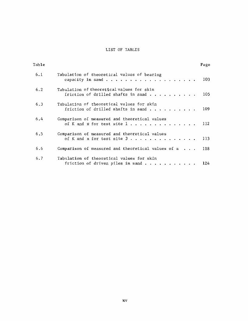
in-situ density or consistency of soils. A standard split spoon sampler is

driven with a l40-lb hammer that is dropped 30 in. The number of blows

needed to drive the sampler 6 in. is recorded for three consecutive 6-in. in-

crements. The blows required to drive the sampler the last two 6-in. incre-

ments constitute the NSPT-value.

The SDHPT cone test is also a dynamic penetration test. In this test a

"standard" cone is driven by a l70-1b hammer that is dropped 24 in. The

number of blows required to drive the cone 6 in. into the soil is recorded

for two consecutive 6-in. increments. The total number of blows for the two

consecutive 6-in. increments constitute the NSDHPT-value.

Correlations between the standard penetration test and the dynamic

SDHPT cone penetrometer tests are given by Touma and Reese (1972) and are as

follows.

In clay:

:::e

NSDHPT = 0.7 NSPT (2.1)

In sand:

z

NSDHPT := 0.5 NSPT (2.2)

The variation of NSPT and NSDHPT with depth for the three borings is

shown in Fig. 2.4.

Besides performing the standard penetration test, McBride-Ratcliff also

performed the pocket penetrometer test and various laboratory tests on the

clay. The laboratory tests performed included consolidation tests, Atterberg

limits, moisture contents, unconfined compression tests, and unconsolidated-

undrained triaxle tests (Q-test).

12

Consolidation tests showed that the clay from 40 to 48 ft was normally

consolidated and the clays below the 53-ft depth were normally consolidated

to slightly overconsolidated. Atterberg limits and moisture contents were

determined at various depths. The results of the index tests can be found in

the boring logs (CB-l and CB-2 in Appendix A). The results of the tests run

to estimate the undrained shear strengths are shown in Fig. 2.5. Included in

this figure are values of the undrained shear strength detern.ined from NSDHPT

AND NSPT values. Correlations between NSDHPT and NSPT values and undrained

shear strength are given by Quiros and Reese (1976) and are as follows.

For homogenous clays (CH):

~

s = 0.07 NSDHPT u (2.3)

or

~

s = 0.10 NSPT u (2.4)

For silty clays (CL):

(2.5)

and/or

(2.6)

For sandy clays (CL):

(2.7)

and/or

(2.8)

13

N, Blows / ft (NSPT and NSDHPT )

0 25 50 75 0

100 125 150 175

• 10 0

0

0

20 EJ 0

0

30 • 0 El

0 - <:. El -.... s::::. 40 (E -Co Q)

0

50 0 S DH PT -I (NSDHPT)

0 IJ CB -I (NsPT ) c. 60 0

El • CB -2 (NsPT ) 0

EJ 0

70 0

EJ 0

80 G

Fig. 2.4 Penetration Resistance as a Function of Depth for Test Site 1

14

Undrained Shear Strength. psf

0 250 500 750 '000 1250 0 I

x Converted Pocket Penetromet (! r

10 • Unconf ined Test .. Q - Test

0 Converted NSPT

8- Converted NSDHPT 20

30 -..... .. .s::. -Q. Q) 0 0 40 x • A

0 x • X A

50 0 • X8-X 8-

.. 0 x xA • • A

60 0 • X ~oo

0 eJQ.24 )(21.00

70 0 ~o

• ~o

Fig. 2.5 Undrained Shear Strength as a Function of Depth. lest Site 1

These equations give the values of the undrained shear strength in tons per

square foot.

Site 2 - Galveston, Texas

15

Site Location. The test at site 2 was also done at The University of

Texas Galveston tledical Branch, Galveston, Texas. This test was done in June

of 1978. The load test was performed in conjunction with the construction of

a parking facility for the Ambulatory Care Center. The location of the pro

posed structure and test site is shown in Fig. 2.1.

Soil Profile. The soil profile at site 2 was determined from two bor

ings, designated as B-1 and B-2. The location of these borings relative to

the proposed structure is shown in Fig. 2.6. The borings were sampled and

logged by personnel of McClelland Engineers, Inc., a geotechnical engineering

consulting firm. The general soil profile is shown in Fig. 2.7. The boring

logs are given in Appendix A.

At both borings the standard penetration test was done to approximately

a depth of 40 ft. Below a depth of 40 ft samples were taken and pocket pene

trometer and torvane tests were performed, along with various laboratory

tests. Laboratory tests that were performed include Atterberg limits,

moisture contents, unconfined compression tests, and unconsolidated-un

drained triaxle tests (Q tests). Atterberg limits and moisture contents

were determined at various depths and the results can be found in the boring

logs in Appendix A. The results of the tests run to estimate the undrained

shear strength are shown in Fig. 2.8, along with the variation of NSPT

with

depth. It should be noted that the NSPT values were not converted to un

drained shear strength because the standard penetration test was run only in

the sand layers.

r---------------------- ---,

I Ambulatory Parking Foci I i ty I I I I I I I I I

I @ 8-1 : I @ 8-2 I

I I I I

: !..r- - ----, L __________________________ • I

L ____ ...J

o 50 100 ft ---- ---- ----- --

. 2.6 Soil Boring Locations, Test Site 2

PC!'

-.....

o ---r.-. -:"T. -:-. "T':" • ..,..,. · . . ~ .' · '. '" .'. ". .' ','

~ :.;.: .... :: .. .' • <

" ' ~ . .' .. . ' .' . . : ' .

I 0 ~.--,J-..:., . ...L.... -.:-t.'

20

.' " .' , . ' . . ' .. · '.' . , .. · .' . · .. ' . '. . .'.

· .' .. '. ' ... · "' .. :,'

.' . . '. ' .. '

Loose to Firm Silty Fine Sand wI Shell Fragments and Some Clay

· . ,' . .' '.1--- Dense to Very Dense Gray Fine Sand .' .: ..

30

'. . .' . '. .~.

' ... ' '.'

.: '. ' .. : · .. ' · : ' . . ~: · . ".

~ . . .' . · . '" ." .~. :~. < : : .. ,'.' '.' *. : · ... ~ .... · '. .. . . ~. ~.

~ . . . . . · .' . .. ' .. ~ ... : a .~ • *

;: 40 · " '"f: "

0. (I)

o

50

60

70

80

'1--- Firm Gray Silty Clay with Numerous Sand Seams

1--_ Stiff ,Tan and Light Gray Very Silty Clay

.2.7 Soil Profile, Test Site 2

17

1.8

--

o

o o

10

20

30

.s::. 40 -a. m 0

50

60

70

80

•

400

10

• • • • ••

•• a

alb

~D

~

Undrai ned Shear Strength, psf

800 1200 1600 2000 2400 2800

20

•

0

0

~

NSPT ' Siows/ft

30 40

•

• •

••

• o • •

50 60 70

• •

•

• •

•

.-NsPT a-Conl/erted Pocket

Pene t rometer

.-Converted Torvane

O-Unconfined Test

A-Unconsol i dated Undrained

.:)

• a

•

Fig. 2.8 Penetration Resistance and Undrained Shear Strength as a Function of Depth, Test Site 2

19

Site 3 - Eastern Site

Site Location. The only information about the location of this site

that can be disclosed is that the test site was in an eastern state. The two

load tests were done in conjunction with the building of three nine-story

structures. The results from these load tests were to be presented to the

designers so that a foundation type could be selected and a final design

could be made.

Soil Profile. The soil profile was determined from three borings, desig

nated as E-l, E-2, and E-3. The borings were done by a testing and engineer

ing company from the same area. Boring E-l was located exactly where the

first test shaft was to be installed. Borings E-2 and E-3 were nearby and

within the perimeter of the proposed building. The second load test was also

located within the perimeter of this building. The standard penetration test

was done at all three borings. The general soil profile is shown in Fig. 2.9

and the variation of NSPT

with depth is shown in Fig. 2.10. The boring logs

are given in Appendix A.

20

-..... .. -a. CD o

o ---"-.. -.-. ..,... .. ....., . .. ' . . Brown and Tan I Medium to Fine Silica

.5L ','::.' .'1--- Sand wI Trace of Limerock ~- .. '

. . .......... "1--_ Tan and Brown,Medium to Fine Silica

10 - ........... : . Sand wI SI ight Trace of RClots

20

. . '. 'I--_Tan,Medium to Fine Silica Sand wI .... : .' Some Limerock and Marl · .' ., .....

.' . · .' .

1--- Brown,Medium to Fine Silica Sand

3 0 ----f-.--,::.-..~ .. --1

.' '.'

· ' .. ' r---Tan,Medium to Fine Silica Sand

4 0 --+----'----1 · . '. .

.' ....

. .. ' Gray, Medium to Fine Silica Sand

50 _ .... ,:'- ..... :-.. ' ..

• • , I

.C?:: '... Tan, Medium to Fine Silica Sand wI : ... 1---

.::.0: Trace of Limerock ..

D" .

·.· .. 0

Gray,Medium to Fine Silica Sand wI .' 0 .. '.1---'. . Some Limerock

70 - .":" .... · . "0.

, '. · . : ··.-0· .~.: ~I--- Gray Limerock wI Si lica Sand "'0'" 80-,·,· .

Fig. 2.9 Soil Profile, Test Site 3

21

NSPT , Blows/ft

00 10 20 30 40 50 60 LhO

~ ~ )0 ~ 0 .41 Jl 0 10 o 0

.~ 6. 6.

~6 6.

20 0 0~ o 0 6. E- 1-0 0 8 LlsI' 0a6.0 E-2-6

0 30 0 0 E-3-0

6.0 6. 0 0 0 0 0 - LD 0 0 'to-~ 0

.s:: 40 0 0 - ~ 6. a. o Q:J CI) 0 0

c:#?6.0 0 0

50 o 0 ~ . c::n 0 0 0

~ 0 ~

60 0 0 ~ 0 6.0 0 0

o L.Ql O 0

6. 0 70 0 0 0 8 6. 0 6.

0 ~ 0~ 6. 0 0 0 80 0 0

Fig. 2.10 Penetration Resistance as a Function of Depth, Test Site 3

CHAPTER 3. INSTRUMENTATION

Measurement of Axial Load at the Top of the Shaft

Axial loads were applied to the top of the test shafts by means of

hydraulic jacks supplied by Farmer Foundation Company and the Texas State

Department of Highways and Public Transportation. The hydraulic jack supplied

by Farmer Foundation Company has a maximum load capacity of 1,250 tons and

was used for load tests at site 1 and site 3. Each of the tWG jacks supplied

by the SDHPT had a maximum capacity of 500 tons and both were used at test

sites land 2. Exactly which jacks were used for a load test will be given

in a later chapter. The loading-system arrangement is shown schematically in

Fig. 3.1. This is the same system that was employed for all the tests, both

at Galveston, Texas and at the eastern site.

The hydraulic jacks that are used in these load tests are not ordinary

jacks, but jacks specifically designed for load tests. For further informa

tion on these hydraulic jacks and their special characteristics, a report

by Engeling and Reese (1974) may be consulted.

The axial load at the top of the shaft was obtained by measuring the

pressure of the hydraulic fluid going to the jack. Measurement of the

pressure was accomplished with both a Bourdon-tube pressure gauge and an

electrical pressure transducer (model BLH GP-CG). Both the Bourdon pressure

gauge and pressure transducer can be seen in the photographs in Fig 3.2. The

transducer allows measurement of pressures to a sensitivity of 10 psi. The

jack pressure is then converted into applied axial load by the use of a

calibration curve.

23

Electrical Pressure Transducer

Bourdon Pressu re -. Gauge (0-5,000 psi)

Air Driven--~ Hydraulic Pump

Air Line\

W Diesel Driven Air Compressor

Hydraulic Oi I Lines

Bour don Pressure Gauge (0-20,000 psi)

Ii; : II: I

Reaction

Piston

500 or 1,250 ton Capacity Hydraul i c Jack

III III IIII1

1IIIt/---Te st Shoft I. :11

(After Bar ker and Reese, 1969)

l(;n 1. 1 Arr":JT""IO'DTTlDnt- ,,-4= T ............ ....:1...:_ ...... C'_._,,- __ • ~b· ..., ............. - ... ·b-~ ... - ...... ~ '-" .... LJVCLU~L15 oJy~Lt::HI

tv ~

25

Fig . 3.2 Photographs of I nstrumentation at Top of Shaft

26

Measurement of Movements at the Top of the Shaft

Vertical movements at the top of the shaft were measured by three dial

gauges. The gauges were located approximately at third points around the

shaft. The dial gauges were mounted on a stationary referenc'e frame as seen

in Fig. 3.2. A typical reference frame is composed of two 1 x 6 timber beams,

each 18 ft. in length. The beams are braced to prevent lateral movement and

supported at each end. Mounted on the reference frame were aluminum gauge

stands (Fig. 3.2) which were used to hold and position the dial gauges over

the top of the test shaft. The dial indicators used were Starrett No. 655-

2041, which have a sensitivity of 0.001 in. and a maximum travel of 2.0 in.

Measurements of Loads at Selected Locations within the Shaft

There are a few different instrumentation systems that are capable of

measuring axial loads in drilled shafts. These systems have been discussed

in detail by Barker and Reese (1969) and O'Neill and Reese (1970). During

the past ten years, because of research done at The University of Texas at

Austin, the Mustran-cell system has been used almost exclusively in instrument

ing drilled shafts to be subjected to axial loads. The term~ustran is an

abbreviation for "Multiplying Strain Transducer." The successful use of the

Mustran cell system has been reported by Barker and Reese (1970), O'Neill

and Reese (1970), Touma and Reese (1972), Engeling and Reese (1974), Wooley

and Reese (1974), and Aurora and Reese (1976). Because of the proven per

formance of the Mustran-cell system, it was used as the only system for

measurement of loads at selected locations within the shafts for this study.

The Mustran-cell system has undergone a few changes since its first use

in 1969, but the theory of its use, as reported by Barker and Reese (1969),

27

is still the same. The Mustran cells used for these tests were a modification

of the Type-2 Mustran cell. The components of a typical Mustran cell used in

this study are shown in Fig. 3.3. The cell is composed of a 1/2-in. square,

steel bar which is tightly screwed at each end into cell caps. Bonded to the

cell column are two 90° rosette strain gauges. The gauges are of the foil

type. A rubber hose with an inside diameter of 1-3/8 in. fits over the 1/2-in.

square, steel bar and is clamped tightly at each end to the cell caps.

Between the cell cap and rubber hose there is silicone rubber glue that is

used as a sealant and helps to make the system air-tight. The interior of

the Mustran cell needs to be kept dry because the electrical resistance of

the strain gauges change erratically in the presence of moisture. The cells

are kept moisture-free by pressurizing the cells with dry nitrogen. The

lead cable of each cell is connected to a sealed manifold. The manifold

is then pressurized with dry nitrogen and the nitrogen is distributed to

each cell through the lead cables. The schematic arrangement of pressuri

zing 11ustran cells through the manifold is shown in Fig. 3.4. The materials

needed and the construction procedure for a Mustran cell are given in

Appendix B. In Appendix C a brief presentation is given of some of the types

of instrumentation that can be employed in drilled shafts to measure the

distribution of axial load with depth.

In the field, before the cells were attached to the reinforcement cage,

each cell was connected to a portable strain indicator to check electrical

continuity, and the resistance-to-ground of each cell was checked with an

ohmmeter. These checks were made to insure that each Mustran cell was

functioning properly before installation.

28

= C\J ...... •

CO

Cell Column (Steel Rod)

C\J ...... I

Beldon Wire 41= 8729

~22 AWG, Stranded 4 - Conducter, J Beldfoi I Shielded , Pla:~tic Jacketed Instrumentation Cable ,0.265 in. 0.0.

wagelok Male Connector =#I: B-400-1 .. 2

Hose Clamp

Rubber Hose 1_3/8 11 I. O.

(Radiator Hose)

Section A··A

Strai n Gauge

[

/411 Foi I Gauge, 90 (TI3e) Rosett e t J Full Bridge, Micro- Measurement Gouge EA-06- 250TG -350

Cell Cop I I

~--lI.,--->I,---C::=::=::==:::.::!:!=::::J ~'/8"

ll-3/8 11 I I I

I 1

{ 2-1/2"~ I 1

(After Barker and Reese, 1969)

Fig. 3.3 Components of i1ustran Cell

Swagelok Male-------.. Co nne c tor c;;==5:E:::::!:;?

#B-600-1-4

Milton Kwik ~ Ch ange Coupler

Ir I

I

29

Pressurized I nst rumentat ion Cable ,Beldon #: 8729,Stranded 4- Con-Lducter 1 Beldfoil Shielded. Plastic

Jacketed ,0.265

Removable Top

Closed

Removable Top

Flexible Tubing

Mustran Cell

4 .'. ~'. ,. '. ,; 4. •

,6

.. "

4' •

" rr II

CI,

, ,

' .

.. .6

inch 0.0.)

Test Shaf t

•• ,,' • • ;J'.o";'

•. <1 ~

. . .0,

' . ,L\

.4

'.:1

v'

ONS Nit rogen ' <I , 0 .; . , .

Cylinder . b', • " ' ~' 4, :" ! 21 4 't>- "

(After Barker and Reese t 1970)

Fig. 3.4 Schematic Arrangement of Mustran Cell Pressurization System

30

After the cells were checked, the cells were installed in the following

manner. Attached to each cell cap was a steel angle made from l/2-in.-wide

and l/8-in.-thick steel strap. The angles were used to mount the cells on

the reinforcing steel using radiator-hose clamps. The cells were mounted

at predetermined depths (distance from top of rebar cage) with two cells at

each depth (level), except the top and bottom levels which had four cells

each. The axes of the Mustran cells were parallel to the axis of the shaft.

At each level the cells were placed on opposite sides of the reinforcing cage.

This was done so that if any bending occurred in the shaft, averaging the cell

readings at a level should eliminate the effect of bending. Therefore, at

any level, the cells were spaced 180 or 90 degrees apart, depending on whether

there were two or four cells. The cells were attached with the Swagelok

fitting facing the bottom of the shaft. The lead cable was then made into

a small loop and taped to the reinforcing steel. The cable was then run along

the length of and taped to the reinforcing bar and out the top of the rein

forcing cage. The procedure for installing Mustran cells is given in

Appendix B. Photographs in Fig. 3.5 show Mustran cells installed on a reb,ar

cage. The relative positions of soil layers and Mustran cells are shown in

Fig. 3.6 for the Galveston tests and for the Eastern tests.

After all the cells were mounted on the reinforcement cage and the lead

wires taped to the reinforcing bars, the lead cables were connected to the

manifold and pressurized. The reasons for pressurizing the system and how

it was done were given earlier in this section. At test site 1 in

31

Fig. 3.5 Photographs of Installed Mustran Cells

Test Site Test Site 2 Test Site 3 w N o .' _.' ,1.1 -~T

0 -~I II I I I 1 T on -0

..... r<l-i- III I I I I I I " , '

-0

0 Lti lotH I.D ' " I I 10 -Li' :1,'1 I I 10 -, , q , , ,

0 -~ ~. >' ':. co

0

''.1'1'''1 I.D '- ,

2 0 -r'I~':'::: I I " '" 10

-10 20 ' ' 20 Iri ' ' ' , _ ~ I I I

I I I I 0 , ."

-:1 0 · ' .. I I " '

I.D ' ,

30 -t,I:',l--1 I I - " , 160' - 30 0 30 ' ' , Lti

0 60' v I I I.D 0

••.. 1. 'I I I _v-t I I I ' ,

-0 ' ' I I ' , 0 , ' , · ...

_v+ I I 40~ ~ 40 .. ' .. -0

80' 40 '. ' .. ' I

I I 0

0 aj .. ', ..:t ~ I I I

~ I I ' , -0

I I ...... _..:t ... I I I

~I 0

50 -l~~ 50 0 50 - .' .. ~:, : . _v f- I I I -

-~t I I I I -

-~1 I I CJ: .. I

I I I I ,'_ '0: ~ I I II 60 -l~~ T 60 60

:~:, - f 10 10

C\J -0 - ': D', ' -

1 I I I

I ,0

70 ~ "'-'1 70 ~ "'-"'I 70 - ' "

, , .....

80~ 80~ :~*Wl m · .' .. : 6<0, , 0',

80 0',0

Fig. 3.6 Relative Positions of Soil Layers and Mustran Cells

33

Galveston, before the manifold was sealed, the wires coming from the lead

cable were soldered to a terminal strip. The terminal strip was then con

nected to a 51-pin, Bendix environmentally sealed female connector, which was

in the end plates of the manifold, as shown in Fig. 3.7. The special manifold

was used in order to keep nitrogen pressure on the Mustran cells during the

load tests.

After pressurizing the Mustran cells, a soap solution was used to check

for leaks in the system.

Testing of Mustran Cells. Tests were done on the Mustran cells

prior to the load tests at test site 1 in Galveston to study the nitrogen

pressure that should be maintained. Prior to the Galveston tests the pressure

had always been set at 20 psi. Earlier that year a load test on a 100-ft-deep

shaft was performed and many of the Mustran cells at the bottom did not

respond. This led to the investigation dealing with the internal pressure

of the cells. The Mustran cells were put inside a triaxial-type set-up, as

shown in Fig. 3.8, so that both the internal pressure of the Mustran cell

and the external pressure around the Mustran cell could be controlled. The

tests showed that the radiator hose used for the Mustran cell started to

collapse inward when the external pressure was 5 psi greater than the inter

nal pressure, as shown in Fig. 3.9. When the external pressure was 20 psi

or greater than the internal pressure, the Mustran cell would short out.

Also, the collapsing of the rubber hose ~n the Mustran cell will change the

stiffness of the cell, making it impossible to compare directly the output

from the varioBs cells. As a result of these tests, it was decided that the

34

Fig. 3.7 Te nni na 1 S trips and Connectors in Nanifold

3S

Fig. 3.8 Must r an Cell in Test Setup

Fig. 3.9 Collaps ed Radiator Hose on Mustran Cell

36

internal pressure of the Mustran cell should be kept greater th~n or equal to

the external pressure on the cell. The external pressure can b~ assumed to

be about 1/2 psi per ft of depth when the excavation is filled 'Nith slurry and

about 1 psi per ft of depth when the excavation is filled with fluid concrete.

Readout System

The output of the Mustran cells was in micro inches per in,::h as indicated

by the recording instruments. Two systems were used for reading the gauges:

1) an automatic data-logging system manufactured by Vishay-Elli:3 (See Fig.

3.10), used for the test at test site 1 in Galveston; and 2) a :3ystem employing

a portable strain indicator and switch-and-balance units (See Fig. 3.11), used

at the Eastern site. It is not known what system was used at test site 2

in Galveston.

The Vishay-Ellis Data Recording System consists of the foLlowing compo-

nents.

0 one VE-20 digital strain indicator

0 one VE-21 switch-and-balance unit

0 one VE-22 data printer

0 two VE-24 switch-and-balance units

0 one VE-2S scan controller

o five gauge terminal blocks

This system requires only one operator and is capable of scanning 40

channels at a rate of approximately one channel per second. The system also

has an automatic printer which records the readings on a paper tape.

37

Fig. 3.10 Vishay Automatic Data-logging System

Fig. 3.11 Portable Strain Indicator and Switch and Balance Unit

38

The second system, consisting of a portable strain indiccctor and

switch-and-balance units, is a manually operated system. For the tests at

the Eastern site three portable strain indicators and three s"'itch-and

balance units were used. Three operators were required, one for each set.

The operator had to switch to a channel (10 channels per switch-and-balance

unit), balance it on the strain indicator, record the readings, and switch

to the next channel. It took approximately one minute to read and record

the ten channels.

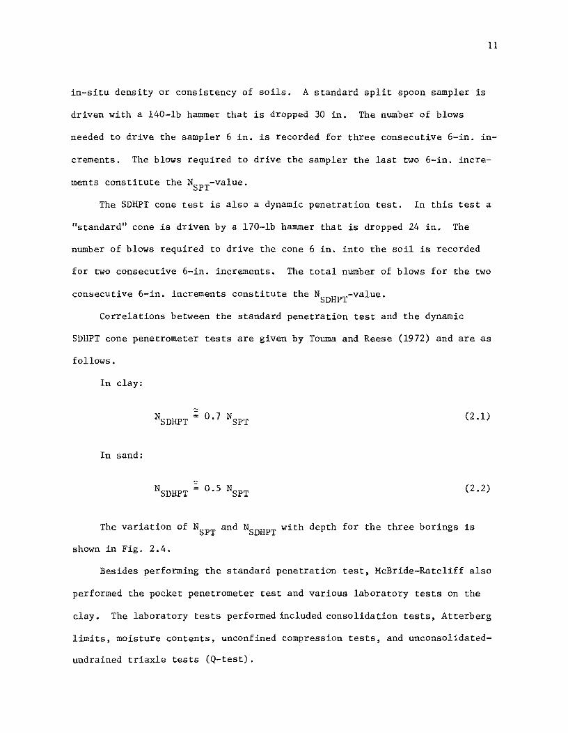
CHAPTER 4. SHAFT INSTALLATION AND CONSTRUCTION PROCEDURES

Test Site 1 - Galveston, Texas

Test Shafts. Three test shafts were constructed at test site 1 in Gal

veston between August 5, 1980 and August 15, 1980. A 48-in.-diameter by 60-

ft-long test shaft, G-l, was constructed by the casing method. The following

procedure was employed. The first step was to drive a 48-in.-diameter casing

with a vibratory hammer to a depth of 52 ft. Then a 46-in.-diameter auger

was used to excavate the soil inside the casing and to advance the hole to

its final depth of 60 ft. At this time it was noticed that water was seeping

into the hole, so a slurry was added to the excavation. A cleaning bucket

was then fitted to the kelly and used to clean the bottom of the hole.

The steel cage for the 48-in.-diameter shaft consisted of eight number

10 bars to 18 ft and four number 10 bars from 18 to 60 ft. The cage, instru

mented with Mustran cells, was lifted with a crane and carefully placed into

the hole. Nitrogen pressure was maintained on the Mustran cells to prevent

any seepage of moisture into the cells.

Concreting of this shaft was done with the help of a tremie which was

lifted and positioned inside the steel cage by means of a crane. The tremie

was filled with concrete by means of a steel hopper. Because of the high

temperatures, between 90 and 100 degrees Fahrenheit, it was decided to add

300 Ib of ice to each 8-yd load to keep the temperature of the concrete down.

This worked quite well; the temperature of the concrete was around 85 degrees

Fahrenheit when it was poured. A slump test was also done and the concrete

39

40

slump was found to range from 9 1/2 to 10 in., which was considered accep

table.

Concrete was trended into the shaft until the level of the concrete was

within a few feet of the top of the shaft. At this time the manifold for the

Mustran cells was placed inside the rebar cage and tied to the cage. The vi

bratory hammer was then connected to the steel casing and the casing was

pulled out. The manifold was removed from inside the shaft and more concrete

was added to complete the construction.

The next shaft constructed was 36 in. in diameter by 65 ft in length,

test shaft G-2. The construction procedure used for this shaft was as fol

lows. A 4S-in.-diameter casing was driven to a depth of 50 ft with a vibra

tory hammer, as shown in Fig. 4.la. A 46-in. auger was then used to exca

vate the casing to its full depth. Slurry was introduced and a 36-in. auger

was then used to excavate the hole to its final depth of 65 ft, as shown in

Fig. 4 .lb. After the excavation was at its final depth, a 36-·in .-diameter

casing was placed in the hole, with the slurry still in the hole as shown in

Fig. 4.lc. The casing went the full length of the hole.

At this time a problem occurred in that sand and water blew into the

hole and the casing started to settle. The sand that was enccuntered was not

indicated on the original soils report. To overcome this problem, cables

from the ~rane were hooked to the casing and the casing pulled plumb and to

its original position. Then the bottom 6 ft of the shaft was filled with

concrete, as shown in Fig. 4.ld. With the crane still supporting the casing,

the concrete was left to set overnight. The next day, with the slurry still

in the hole, the concrete in the casing was augered out to a depth of 60 ft.

A reinforcing cage consisting of eight number 10 bars to IS ft and four

number 10 bars to 60 ft was placed into the hole. This cage was

48U

t/J Steel Casing

(Driven)

50 1 4.c IJrJR

(a)

481

Casi

(Augered

65

t/J 19 Out

S

3 A

( b)

urry

:::j jj~~ ,,::~

I .... J

~ :.;i

ii~~~~

"

I ::~1

II 6" t/J gered Hole

(c)

Fig. 4.1 ?1ethod of Construction of Test Shaft G-2 at Test Site 1 (a) Driven (b) Drilling Below Casing with Slurry; (c) Placement of Inner Casing

II f:

I! p:

I ~""

M ;r;:jj, 36"t/J)( 651

j~!~ Steel Casing

,!jj~: ~ .•. l~~l

~!I~ ~." '.:?

~ t-

48" ~ Casing

65 1 .' 'mJ'K

(d)

Slurry

36"~ x 65' Casing

61

Concrete Plug

,b.' A'

:~ ,~

':;' .6 ' CfID(" •

(e)

"',-'Iii;

36"~ x65' Casing

'A ,',

': :,' 4 ': A' '

,_. 4 4.-

L,),: ','-

. '

• ' './I.' :, '"

(f)

Slurry

Fig. 4.1 Hethod of Construction of Test Shaft G-2 at Test Site 1 (con'd) (d) Concrete Plug Poured; (e) Placement of Concrete; (f) Completed Shaft

-+:'I'..)

43

uninstrumented. With the 48-in.-diameter casing still in place, the concrete

for this shaft was placed with the aid of a tremie, as shown in Fig. 4.le.

As with the 48-in.-diameter shaft, 300 lb of ice were added to each 8 yd of

concrete. Slump tests were done and the concrete slump was found to range

from 9 1/2 to 10 in. The 36-in., steel casing was left in place on this

shaft, but the 48-in. casing was removed and the slurry was left between the

casing and the soil. By the next day the soil at the ground surface had

moved inward toward the casing. Figure 4.lf presents an estimate of the

final configuration of the casing, slurry, and excavation.

The third test shaft, G-3, constructed was 36 in. in diameter by 60 ft

in length. The following construction procedure was used. A 42-in.-diameter

surface casing was driven to a depth of 10 ft. Then a 36-in.-diameter hole

was augered, with the use of slurry, to a depth of 35 ft. At this time a

36-in.-diameter casing was screwed in to a depth of 40 ft. The excavation

was then continued, with a 34-in. auger and slurry, to a final depth of 60

ft.

The steel-reinforcing cage for this shaft consisted of eight number 10

bars to 18 ft and four number 10 bars from 18 to 60 ft. The cage, fully

instrumented, was lifted by a crane and carefully placed into the hole.

Nitrogen pressure of approximately 55 psi was maintained on the Mustran cells

to prevent any seepage of moisture into the cells.

Concrete was placed in the shaft with the aid of a tremie and steel

hopper. The shaft was filled completely with concrete and the casing was

left in place. As in the previous shafts, 300 lb of ice were added to each

8 yd of concrete. Slump tests were performed and the concrete slump was

found to range from 9 1/2 to 10 in. The last step was to remove the 42-in.

surface casing.

44

Grouting of Test Shafts. The two 36-in.-diameter test shafts were

tested on September 4 and 5, 1980. The instrumented, 36-in.-diameter shaft

(G-3) was tested on September 5. As expected, because of the easings being

left in place, the shafts failed at relatively low loads. The results of

these tests will be discussed in a later chapter. In an attenpt to increase

the load-carrying capacity of the shafts, it had been previously decided to

grout around sections of each of the 36-in.-diameter shafts.

The grout that was used for both shafts was supplied by Sullivan Enter

prises in Galveston (quality control no. 740-1271). The mixture for one

cubic yard of grout consisted of 750 Ib of sand, 846 Ib of cement, 40 Ib of

water, 27 oz of normal-set water reducer. Water was then added on the job

site to get a workable fluid mix. A single-cylinder grout pump was used to

inj ect the grout. Although the grout pressure was not measured, it is

assumed that it was low.

Grouting of the 36-in.-diameter shaft, (G-3) with a casing to 40 ft was

as follows. Six grout tubes were j ettedinto place, three to a depth of 40

ft and three to a depth of 30 ft. Grout was then pumped into the tubes, and

pumping was continued as the grout tubes were removed. A total of 8 cu yd of

grout were used to grout the shaft from the ground surface to a depth of 40

ft. Assuming that the excavation in the top 40 ft, using the 36-in.-diameter

auger, had a diameter of 37 in., the volume of the annular space around the

casing was 0.6 cu yd. Therefore, the volume of grout was abo1.Lt 13 times

greater than the annular space.

The grouting of the 36-in.-diameter shaft (G-2) with a casing to 65 ft

was done in the following manner. Three grout tubes were jetted to a depth

of 65 ft. Then a total of 6 cu yd of grout was pumped into the grout tubes,

puraping was stopped, and the grout tubes withdrawn. After the grout had been

45

allowed to set, a steel rod was used to learn the extent of the grouting. It

was determined that the lower 15 ft of the shaft had been grouted. The volume

of the annular space around the casing of the lower 15 ft, using the same

assumptions indicated above, was about 0.3 cu ft. Therefore, the volume of

grout was about 27 times greater than the annular space.

The amount of grout used around the drilled shafts, 8 and 6 cu yd, is

con~idered to be quite large for the area that was grouted. No information

is available about what happened to the excess grout that was used. It is

unlikely that the diameter of the annular space around the shaft was in

creased uniformly. The most likely possibility is that the soil was frac

tured and that the grout flowed into a weak zone in the soil. Elevations

of the three test shafts prior to grouting, but shoWing the area to be grou

ted, are shown in Fig. 4.2.

Shafts. Four reaction shafts were constructed at test site 1 ~~~~~~~~

in Galveston. All four reaction shafts were 48-in. in diameter by 60 ft in

length with a 96-in. underream. Each shaft contained twelve 1 in. by 60 ft

dywidag bars. The following general procedure was employed for the construc

tion of the four reaction shafts. The first step was to drive a 48-in.

diameter casing with a vibratory hammer to a depth of 52 ft. A 46-in.

diameter auger was then used to excavate the soil inside the casing. When

the excavation reached the bottom of the casing, water began to seep in, so

a slurry was added to the excavation. The excavation was then advanced to

its final depth of 60 ft. At this time a belling tool was used to add a

96-in. underream to the bottom of the shaft. The dywidag bars were then

lifted with a crane and placed into the hole.

Concreting of the reaction shafts was done with the aid of a tremie and

steel hopper. The tremie was lifted and placed inside the excavation with a

V,

tJ

, ,1>

Q,

48 11 cp • 4'

II

, ,

J)

b ~

, 4,

, ~,

52 1 _ ',A,

46"ct> L.~: 60 1 I"b" 772

Test Shaft G-1

Fig. 4.2

:..

*

, ,', b, :I'i :~, <I ~,:~ ~l . . .. .', ","

;~' A

36"cp X6~I'; , ',:' ,l . . " ' ~

Casing '," 4':1 ~ , :',', ~ ~;

50'- -

:I,~ : , ' ~;: , r.:::

~:'

,;l.~, .. , 'l: ;~~ ',: ~,t

,J-

,A

~',' ,

.. '~

651 __

rbJ

"~ .. 4·1~ d. '

, ' ,

, /J . 0,

f>'

t:.

Slurry Slurry t-3611cpx40~ ~ .. ,', ,: (Test I)

Casing -.Jil ' , A , f~ Grouted Zone

b '.: U 0-40 1

(Test 2) u . , ll'

4o!- - I " I _ _ _ 1 , 4,1

Grouted Zone 50 1

- 65 1

(Test 2) 60 1

<2' ..

"

~

4 ,~

4 " ' , ~ [< ~

"""~.

Test Shaft G-2 Test Shaft G-3

Elevation of 7est Shafts at Test Site 1, Galveston

J:-C]\

47

crane. The concrete, which had a slump of 9 in., was tremied into the shaft

until the level of the concrete was at the top of the shaft. At this time,

the 48-in.-diameter casing was pulled with the vibratory hammer. Then more

concrete was added to complete the construction.


Test Shaft. A single test shaft, G-4, was constructed at test site 2 in

Galveston. The shaft was constructed on June 7, 1978 with the following pro

cedure. First, a 24-in.-diameter by 40-ft-long casing was driven to a depth

of 40 ft with a vibratory hammer. Excavation of the soil within the casing

was then done with a 22-in.-diameter auger. The excavation was then flooded

with slurry and the hole was advanced to its final depth of 80 ft. A clean

ing bucket was then fitted to the kelly and used to clean the bottom of the

excavation.

The steel cage for the shaft consisted of six number 6 bars extending

the complete length of the shaft. The cage, instrumented with Mustran cells,

was lifted with a crane and carefully placed into the hole. Nitrogen pres

sure was maintained on the Mustran cells to prevent any seepage of the mois

ture into the cells.

Concrete for the shaft arrived at the site and a slump test was per

formed, with the slump being approximately 4 to 5 in. It was decided that

this slump was too low, so more water was added, producing a high slump.

Concrete was then placed in the shaft with the aid of a tremie. In order to

prevent contamination of the concrete in the tremie with drilling mud, a ply

wood plate was loosely fastened to the bottom of the tremie. The hydrostatic

pressure of the concrete in the tremie was not sufficient to push this plate

from the end of the tremie. In order to free the plate and initiate concrete

48

placement, it was necessary to "yo-yo" the tremie several tim,~s. This may

have damaged some of the Mustran cells.

When the level of the concrete had reached the top of th,~ shaft, it was

noticed that the concrete again had a very low slump, possibly 3 in. This

low slump may have been a result of time or possibly bad cement. After the

concrete level was at the top of the shaft, the casing was vibrated out a

distance of 5 ft. At this time the casing was filled with concrete and pulled

completely out.

After the casing was pulled, it was found that the lead \Jires to two

Mustran cells had been pulled from the manifold. Thus, the nitrogen pressure

in the system was temporarily lost until the two lead wires w(~re reconnected

to the manifold.

Reaction Shafts. The construction procedure for the two reaction shafts

at this site is not known. It can be assumed that it was similar to the pro

cedure used for the test shaft. The reaction shafts at this Bite were 30 in.

in diameter by 80 ft in length with a small diameter bell at the end. The

size of the bell is not known.

Test Site 3 - Eastern Site

Test Shafts. Two test shafts, E-l and E-2, were constructed at test

site 3 between January 11, 1981 and January 29, 1981. A 36-in.-diameter by

60-ft-long shaft, E-l, was the first test shaft constructed. The following

procedure was employed. First, a 36-in.-diameter by 60-ft casing was driven

to a depth of 60 ft but, due to densification of the sand and side resis

tance (skin friction), the casing could only be driven to 40 ft at this time.

The 20 ft of casing that was above the ground surface was then cut off and a

34-in. auger was used to excavate the soil inside the 40 ft of casing in the

49

ground. The excavation of the soil on the inside of the casing was done to

eliminate some of the skin friction. The 20 ft of casing that was cut off

was then welded back on to the rest of the casing, the vibratory hammer at

tached, and the casing driven to the final depth of 60 ft. The 34-in.-dia

meter auger was then used to excavate the remaining 20 ft of soil inside the

casing. When augering at the bottom of this shaft, limestone cobbles (8 to

10 in. in diameter) were encountered.

The reinforcing cage, instrumented with Mustran cells, was then lifted

with a crane and carefully placed in the hole. The steel reinforcing cage

for this 36-in.-diameter shaft consisted of eight number 8 bars and eight

number 6 bars. All the reinforcing bars went the complete length of the

shaft.

Concreting of this shaft was done with the aid of a tremie, which was

lifted with a crane and positioned inside the steel cage. A concrete pump

was then used to get the concrete inside the tremie. A slump test was done

and the concrete slump was found to range from 8 1/2 to 9 3/4 in., which was

acceptable.

Concrete was tremied into the shaft until the level of the concrete was

within a few feet of the top of the shaft. At this time, the tremie was re

moved and the manifold for the Mustran cells was placed inside the rebar

cage and tied to the cage. The vibratory hammer was then connected to the

steel casing and an attempt was made to pull the casing. This first attempt

failed so a 50-ton crane and a 2s-ton cherrypicker were added to the 50-ton

crane already being used to pull on the vibratory hammer and casing. This

second attempt also failed. At this time the engineer on the project decided

that they would try to recover the instrumentation so an attempt was made to

50

pull the reinforcing cage out. This also failed. The casing and instrumen

tation were both left in place.

The next shaft constructed, E-2, was also 36 in. in diamHter by 60 ft in

length. This shaft was constructed because the company for which the test

was being done would not accept a test on a cased shaft. The construction

procedure used for this shaft was as follows. A 36-in.-diameter by 60-ft

long casing was driven with a vibratory hammer until the casing broke at a

weld. Information is not available about the exact depth at \oThich the casing

broke, but it was within a few feet of the final depth of 60 ft. The inside

of the casing was then excavated with a 34-in.-diameter auger.. The casing

was then welded back together and driven to the final depth of 60 ft. The

remainder of the soil was then excavated.

'i'he reinforcing cage, instrumented with Mustran cells, was then lifted

with a crane and carefully placed inside the casing. The steel cage for this

shaft consisted of eight number 8 bars. Before concreting of the shaft be

gan, the vibratory hammer was attached to the casing and it was pulled up a

foot or so just to make sure they would be able to pull this casing. Con

crete was placed in this shaft in the same manner as the first test shaft at

this site, with a tremie and concrete pump. The slump of the concrete used

for this shaft ranged from 9 1/2 to 10 inches.

Concrete was tremied into the shaft until the level of the concrete was

within a few feet of the top of the shaft. The tremie was thEm removed and

the manifold was tied to the reinforcing steel inside the casing. The vi

bratory hammer was then connected to the casing and the casing was pulled up

approximately 10 ft. More concrete was then pumped into the casing and the

casing was then pulled completely out. The manifold was then removed from

inside the shaft.

51

Reaction Shafts. At test site 3 four reaction shafts were constructed.

All four of the reaction shafts were 36 in. in diameter by 65 ft in length.

Each reaction shaft had twelve 1 in. by 60 ft dywirlag bars in them. The

following general procedure was used in constructing the reaction shafts.

The first step was to drive, with a vibratory hammer, a 36-in.-diameter cas

ing to refusal, which usually occurred at a depth of approximately 55 ft.

The interior of the casing was then excavated with a 34-in. auger. After the

inside of the casing was excavated, the casing was driven to the final depth

of 65 ft. The inside of the casing was then excavated to the final depth.

Limestone cobbles (8 to 10 in. in diameter) mentioned earlier were encoun

tered when excavating almost all the reaction shafts, usually between depths

of 55 and 65 ft. The dywidag bars were then lifted with a crane and placed

into the hole.

Concreting of the reaction shafts was accomplished with the aid of a

tremie and concrete pump. The concrete was tremied into the shaft until the

level of the concrete was near the top of the shaft. At this time the vibra

tory hammer was attached to the casing and the casing was pulled out approxi

mately 10 ft. More concrete was added and the casing was pulled completely

o~.

CHAPTER 5. LOAD TESTS

Test Procedure

The method used to apply the axial loads to the test shafts was essen

tially the State Department of Highways and Public Transportation "quick

load" procedure. Fuller and Hoy (1970) reported that results from tests per

formed using the "quick-load" procedure, in most instances, agree closely

with results from tests using the more common "maintained-load" procedure.

Essentially, the "quick-load" test requires that loads be applied in equal

increments with gross settlement, loads, and Mustran cell readings recorded

immediately before and after the application of each increment of load. Each

increment of load is held for the same amount of time and then the next load

is applied.

When the load-settlement curve obtained during the test shows that the

shaft has been failed, that is, that the load on the shaft can only be held

by continuous pumping of the hydraulic jack and the shaft is being driven

into the ground, a final set of readings is taken and pumping is stopped.

After the shaft has come to equilibrium, the shaft is unloaded in equal

decrements of loads with settlement readings being taken when movement on the

dial gauges is negligible. When all the load is removed and the shaft has

been allowed to recover, net settlement readings are taken.

The procedure described above follows the SDHPT procedure closely, but

there are a few minor exceptions. The SDHPT procedure states that the time

interval be two and one-half minutes between application of load increments.

53

54

At test site 1 in Galveston the interval was three minutes, and at the Eastern

site it was four-minutes. There is no information of the time interval used

at test site 2 in Galveston. Also, the SDHPT procedure recoDmlends readings

immediately before and after the application of each load. At: the Eastern

site only one set of readings was taken. These were started ]0 seconds after

the load was applied. Only one set was taken because the readings were being

taken manually with switch-and balance units. The SDHPT procedure recommends

that unloading be done in One step (Le., all of the load removed at once);

for these tests the unloading was done in decrements.


Test Arrangement. The testing arrangement at this site consisted of

four reaction shafts and three test shafts. The reaction shafts were all 48

in. in diameter by 60 ft in length, with a 96-in. underream. These shafts

were to be incorporated into the foundation of the building.

The three test shafts consisted of two instrumented shafts and one unin

strumented shaft. The first test shaft, which will be designa.ted G-l, was

48 in. in diameter by 60 ft in length. This shaft was instrumented. Test

shaft 2, designated as G-2, was an uninstrumented shaft that ~'as 36 in. in

diameter by 65 ft in length, with a casing extending the full length of the

shaft. Test shaft 3, designated as G-3, was 36 in. in diamete:r by 60 ft in

length, with a casing extending from the ground surface to a depth of 40 ft.

This shaft was also instrumented. The arrangement of the test shafts with

respect to the reaction shafts is shown in Fig. 5.1.

Test Results

Test Shaft G-l. The load test of test shaft G-l was performed on August

26, 1980, nineteen days after construction of the shaft. The test was begun

,.... 25' a" - ~I "C c: - c

'" -C\I .... /' -en I

I I

I \

\

" .....

36"c:p x65' Test Shaft - Cased 65' I

(Grouted Lower 15' )

-~

en -,....

Typical Reaction \ Shoft- 4 a"c:p x 60' wi 96 II Underream

/'

\

"-"

...... "- ,

\

/ 4a" c:p x 60' /

'" Test Shaft

/'

'" I

I /

(No Casing)

121_ 10"

/ I

I

I

\

'" /

\ , " " ......

36 "c:p x 60' Test Shaft -Cased 40'

(Grout to Surface)

.... ('

I

t-

\ \ ', ...... T

. 5.1 Testing Arrangement, Test Site 1

......

"

,. ....

.....

,

/

"-

61'- 2" To Sixth Sf.

\ \

I

I I

-CX)

v "., C\I

\

I

/ ,. ....

I..n I..n

56

at 2:20 p.m. A seating pressure of 500 psi was applied to the hydraulic jack.

The jack had a capacity of 1250 tons. The pressure on the jack was then in

creased to 1000 pSi, after which it was increased in 200 psi (15 ton) incre

ments to failure, which occurred at 6775 psi. The pressure at failure was

equivalent to a load of 495 tons.

The time to load the shaft was approximately one hour and 20 minutes.

After attaining the ultimate capacity, the shaft was unloaded in 1000-psi

(75-ton) decrements. Unloading began at 3:55 p.m. and took approximately

20 minutes.

The load-settlement curve (all load-settlement curves will be the applied

load and the average settlement at the top of the shaft) is shown in Fig. 5.2.

As indicated in the figure, the maximum load was 495 tons and the maximum

settlement was 1.94 in. Upon unloading, the shaft rebounded and the permanent

settlement was 1.70 in.

Test shaft G-2 was load-tested for the first time on

September 4, 1980, 21 days after construction of the shaft. Unless otherwise

noted, a 500-ton jack was used for this and subsequent tests. An initial

pressure of 750 psi was applied to the hydraulic system. The :)ressure on the

jack was then increased to 1000 psi; the pressure was then inc:reased in 200-

psi (5-ton) increments to failure. The pressure at failure was 3400 psi,

which is equivalent to a load of 81 tons. After the ultimate eapacity of the

shaft had been reached, the shaft was unloaded in three decremlmts of approx

imately 1000 psi (26 tons) each.

On September 11, 1980 the lower 15 ft of test shaft G-2 was grouted.

The grout was allowed to cure for seVen days. The second load test on shaft

G-2 was performed on September 18, 1980. In this test an initial pressure of

o 100

. .5 c

-c E 1.0 CD --CD

(J) 1.5.

I -..:...0--=

2.0

Load, tons

200 300

'=' 0- 0- -0

Fig. 5.2 Load Settlement Curve, Test Shaft G-l

400 500 --,

Max. Load~ 495 tons ~

V1

"

58

500 psi was applied to the loading system. The pressure was I:hen increased

to 1000 psi, and then increased in 400-psi (lO-ton) incrementl; to failure.

The pressure at failure was 14800 psi, which is equivalent to a load of 373

tons. The complete test, loading and unloading, lasted appro~dmately 1 1/2

hours.

The load-settlement curves for both of the tests on test shaft G-2 are

shown in Fig. 5.3. As indicated in the figure, the maximum load in test 1

was 81 tons and the maximum settlement was 1. 69 in. After unloading in test

1, the shaft rebounded and the permanent settlement was 1. 60 in. In test 2,

after grouting, the maximum load was 373 tons and the maximum settlement for

the test was 1.58 in. After unloading and rebound, there was a permanent set

tlement of 1.29 in. with reference to the position of the shaft at the be

ginning of test 2.

Test Shaft G-3. The first load test of test G-3 was performed on Sep

tember 5, 1980, 20 days after the shaft was poured. An initial pressure of

750 psi was applied to the jacking system. The pressure was then increased

to 1200 psi. From 1200 psi to failure the pressure was increased in 400-psi

(lO-ton) increments. Failure occurred at a pressure of 8400 pSi, which is

equivalent to a load of 209 tons. After the ultimate capacity of the shaft

had been reached, the pressure was released in four decrements of approxi

mately 2000 psi (51 tons). The complete test, loading and unloading, lasted

about two hours.

The top 40 ft of test shaft G-3 was then grouted on September 10, 1980.

The grout was allowed to cure for seven days. The second load test of shaft

G-3 was then performed on September 17, 1980. In this test an initial pres

sure of 500 psi was applied to the loading system. The pressure was then

C

-c CD E CD

CD C/)

o o

1.0

2.0

3.0

100

Test I

Load I tons 200

Maximum Load 81 tons

300 400

Fig. 5.3 Load Settlement Curves, Test Shaft G-2

59

60

increased to 1000 psi, and then the pressure was increased in 400-psi (10-

ton) increments until the shaft failed. The pressure at failure was 16,800

psi, which is equivalent to a load of 424 tons. After failul~e the shaft was

unloaded in pressure decrements of approximately 4000-psi (102 tons). The com

plete test, loading and unloading, lasted about two hours and 45 minutes.

The load-settlement curves of the load tests performed on test shaft

G-3 are shown in Fig. 5.4. As indicated in the figure, the laaximum load in

test 1 was 209 tons and the maximum settlement was 1.23 in. After unloading

and rebound, the permanent settlement of the shaft was 1.11 in. In test 2,

after grouting, the load at failure was 424 tons and the maximum settlement

for the test was 1.88 in. Upon unloading, the shaft rebounded and there was

a permanent settlement of 1. 71 in. with reference to the position of the shaft

at the beginning of test 2.

Test Site 2 - GalVeston, Texas

Test Arrangement. The testing arrangement at this site consisted of two

reaction shafts and one test shaft. The reaction shafts were both 30 in. in

diameter by 80 ft in length, with a small underream (exact size of underream

is not known). The test shaft, designated as G-4, was 24 in. in diameter by

80 ft in length. This shaft was instrumented. The arrangement of the two

reaction shafts and the test shaft is shown in Fig. 5.5.

Test Results (G-4). Detailed information on this load test, such as the

exact date of the test, load increments used, permanent settlement, and dura

tion of test, are not available. It is known that the test was run in June

of 1978 and that the shaft plunged at an axial load of 225 tons. Figure 5.6

shows the curve giving settlement of the top of the shaft as a function of

axial load.

o o

. c

I.°k

-c CD E Q) --

100

0 (:).

Load, tons

200

Test I

300

I Max imum Load 209 tons

400

~ 2.0

Test 2

r"""'0 Maximum Load

3.0 0- 424 tons 0-~-___ ~

Fig. 5.4 Load Settlement Curves, Test Shaft G-3

0' 1-'

f---____ 7 1_6 11 7 1-6"

I ~/

,. - '-TYPiCal Reaction

Shaft: 30"" x 801

With Small Underream

24"4> X 801

Test Shaft

Fig. 5.5 Testing Arrangement, Test Site 2

-,-- ...

I

aN

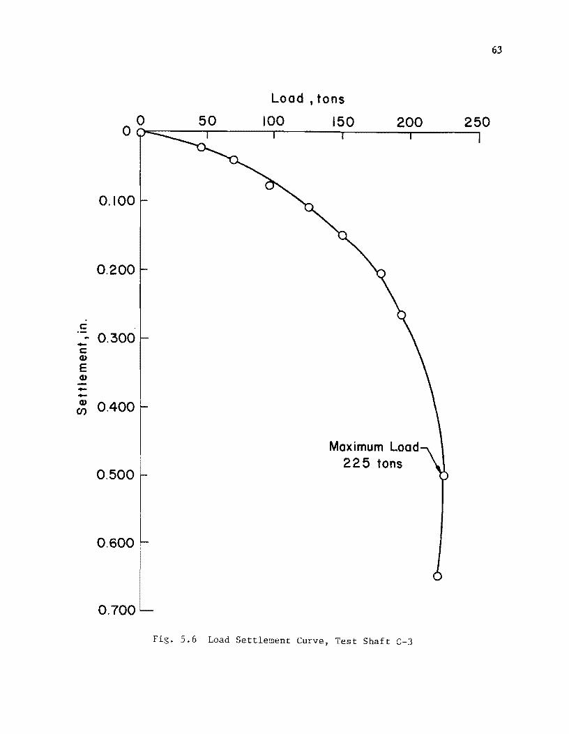
63

Load t tons

o O~~----'-------'--------r-------r-------.

50 100 150 200 250

0.100

0.200

c .-0.300 ... -c

CD E CD --CD 0.400 CJ)


0.500

0.600

0.700

. 5.6 Load Settlement Curve, Test Shaft G-3

64

Test Site 3 - Eastern Site

Test Arrangement

The testing arrangement at this site consisted of four reaction shafts

and two test shafts. All four reaction shafts were 36 in. in diameter by 65

ft in length. The first test shaft, designated as E-I. was 36 in. in diame

ter by 60 ft in length, with a casing extending the full length of the shaft.

The second test shaft, designated E-2. was also 36 in. in dianeter by 60 ft

in length. but had no casing. The testing arrangement of the Eastern site is

shown in Fig. 5.7.

Test Results

Tes t Shaft E~l. The load test of test shaft E-l was performed on Feb

ruary 2, 1981, twenty days after construction of the shaft. The test was

started at 2:45 p.m. A seating pressure of 500 psi was appli.3d to the hy

draulic jack. The hydraulic jack being used had a capacity of 1250 tons.

The pressure on the jack was then increased to 1000 psi after which it was

increased in 400 psi increments (approximately 30 tons) increments to failure.

Failure occurred at a jack pressure of 4800 psi which was equ:lvalent to a

load of 345 tons.

The time to load the shaft was approximately 45 minutes. After attain

ing the ultimate capacity, the shaft was unloaded in 1000 psi (59 ton)

decrements. Unloading began at 3:40 p.m. and took apprOXimately 20 minutes.

The load-settlement curve for the top of the shaft is shown in Fig. 5.8.


settlement was 1.06 in. Upon unloading, the shaft rebounded and the perma

nent settlement was 0.92 in.

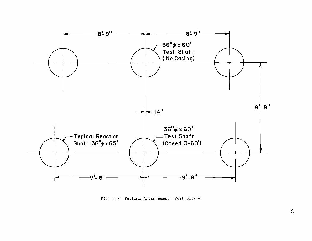
, ., 8 ~ 9" 110 I III 8 1- 9" ~ ,

Typical Reaction Shaft :36"4> x 65

1

36"4> X 601

Test Shaft ( No Casing)

14"

36"4> X 60 1

Test Shaft (Cased 0-601

)

I'III!I 9 1- 6" ~I" 9 1

- 6" ... ,

Fig. 5.7 7esting Arran8ement, Test Site 4

9 1-8 11

'" \J1

c:

-c: CD

E CD --CD

CJ)

o 100

Load, tons

200 300 01 0 ,0 ~ =e- ~

.25

.50

.75

Ma xi mum Load 345 tons

I ~ 1.00

1.25 L Fig. 5.8 Load Settlement Curve, Test Shaft E-l

400

0\ 0\

67

Test Shaft E-2. The shaft E-2 was load-tested on February 4, 1981,

eight days after construction of the shaft. The test was started at 11:15

a.m. A seating pressure of 500 psi (equivalent to a load of 21 tons) was

applied to the hydraulic jack. The hydraulic jack being used had a capacity

of 1250 tons. The pressure on the jack was then increased to 1000 psi, after

which it was increased in 400-psi increments (approximately 30-ton increments

of load) to failure. Failure occurred at a jack pressure of 11,700 psi which

was equivalent to a load of 865 tons.

The time to load the shaft was 1 hour and 55 minutes. After attaining

the ultimate load, the shaft was unloaded in 3000-psi (2l0-ton) decrements.

Unloading began at 1:15 p.m. and took approximately 15 minutes.

The load-settlement curve for the top of the shaft is shown in Fig. 5.9.


settlement was 1.90 in. Upon unloading, the shaft rebounded and the perma

nent settlement was 1.56 in.

As mentioned previously, the reaction shafts for the tests at the Eastern

site were 36 in. in diameter by 65 ft in length, only 5 ft longer than the

test shafts. Because of the reaction shafts being only 5 ft longer than the

test shaft and the construction problems mentioned in the previous chapter,

the movemen~ of the reaction shafts were monitored. The uplifts of the reac

tion shafts were measured by a single dial gauge on each shaft. During the

load test of shaft E-l, there was no significant movement, but during the

load test of shaft E-2, one reaction shaft moved 1.68 in. and the other moved

2.17 in. The load-uplift curves for the reaction shafts used in the load

test of shaft E-2 are shown in Fig. 5.10. The load on each reaction shaft is

one-half the load on the test shaft. The movements of the reaction shafts

68

gave additional information on resistance in skin friction. This information

will be discussed in a later chapter.

c:

-c:

o 100 0, ~

0.5

Q)

E 1.0 CD --CD

Cf)

2.0

Load, tons

200 300 400 500 600

Fig. 5.9 Load Settlement Curve, Test Shaft E-2

700 800


900

0'\ 100

2.0

c

-- 1.0 Q.

:::>

o o 50 100 150 200 250 300 350 400 450

Load, tons

• 5.10 Load Uplift Curves for Reaction Shafts, Test Site E-2

"'-J o

CHAPTER 6. ANALYSIS AND DISCUSSION OF LOAD TESTS

Method of Analysis

Mustran Cell Behavior. The first step in the reduction of the data was

to determine if any of the Mustran cells were operating improperly. The

changes in Mustran cell readings (change from Hustran cell reading when load

was zero) were plotted versus the applied load. For comparison purposes,

all the readings of Mustran cells at a particular level were plotted on the

same sheet. Best-fit curves were then drawn through the readings from each

cell to eliminate any small erratic behavior in the readings. The slopes

of these curves are a function of the shaft properties and of the load trans

fer characteristics of the shaft. These curves were then examined and any

Mustran cell exhibiting behavior that was obviously in error was eliminated.

Observations concerning these curves are discussed in detail by Touma and

Reese (1972). Finally, an average curve was drawn for each level of Mustran

cells. These average curves were then used to determine the load at the dif

ferent levels throughout the shaft.

Calibration of Mustran Cells. The purpose of the top level (calibration

level) of Mustran cells was to establish a response curve relating the load

in the shaft to the Mustran cell readings. The Mustran cells near the top

of the shaft were used for calibration for two reasons:

1. The load at the calibration level is known because there is no load

transfer above the level of the calibration cells.

71

72

2. The dimensions of the shaft near the ground surface are known

accurately.

The calibration curve is then used to convert the readings of Mustran cells

at other levels into units of load by assuming that there is a uniformity

in the properties of the shaft at each level of Mustran cells.

There are instances when it is known that the properties of the shaft at

a particular cell level are not the same as at the calibration level. One such

instance is when the diameters are not the same. This occurs on occasions

where a casing is used in the construction of part of the shaft. The dif-

ference in diameters can be compensated for by adjusting the calibration

curve. Adjustment is done by taking the Mustran cell reading:, from the

calibration curve, for different loads, and multiplying them hy the ratio

of the stiffness of the shaft at the calibration level to the stiffness of

the shaft at the level with a smaller diameter. This is ShO~l in the follow-

ing equation:

(6.1)

where

Mustran cell reading from original calibration curve ,

R2 = adjusted Mustran cell reading for new calibration curve,

EAl stiffness of shaft at calibration level, and

EA2 stiffness of shaft at Mustran cell level of lesser

diameter.

The adjusted calibration curve is then used for the Mustran cells that are

in that part of the shaft with a different diameter.

Also, the shaft properties are not the same at all levels if there is

a difference in concrete strength with depth. An example of this is shown

in Fig. 6.1. This plot was constructed from unpublished data obtained from

the Corps of Engineers. The data are from results of tests of cores from

seven different shafts. The plot shows that there is a maximum difference

of 2 ksi over a depth of 50 ft. The increase in strength is due to two

effects, (1) curing of concrete below the water table and, (2) an increase

in strength with depth due to increasing pressure. The possible difference

in shaft property with depth is not considered in the analysis described

herein because such data as shown in Fig. 6.1 were not available. Further

more, if cores had been taken from the test shafts with results as shown in

• 6.1, corrections would not be very significant.

Load-Distribution Curves. After the calibration curve and individual

73

curves for the Mustran cell readings at the various depths have been plotted,

the loads at the different levels within the shaft were determined for each

chosen load. Once the load in the shaft was known for each level of Mustran

cells, a curve of the load versus depth was plotted. A plot of the load

versus depth is known as a "load distribution" curve.

Tip Load. Tip resistance developed at each load was read directly from

the load-distribution curves that were calculated for each test. Once the

tip load was known, a unit value was calculated by dividing the total load

resisted at the tip by the shaft area at the tip, as shown in Eq. 6.2:

74

Uncon'fined Compressive Strength of Concrete, ksi

o 2 3 4 5 o

10 o 0

20 0

- 0 .... 0

.c. 0 -~ <::J

CD 0 30 0

0 0

0

40 (;) 0

0

50

Fig. 6.1 Variation of Concrete Strength as a Function cf Depth

q Total load resisted at tip Shaft area at tip

(6.2)

After the unit value of tip resistance was calculated, a curve showing the

unit tip resistance versus tip movement was plotted. The procedure for

computing tip movement will be discussed later.

75

Side Resistance. The total load carried in side resistance (skin friction)

was determined by subtracting the load carried at the tip from the applied

load. The load transfer is the load per unit area transferred to the support-

ing material and can be computed at any point from the slope of the load-

distribution curve at that point. In this report, values of load transfer

were calculated over ten-foot intervals along the length of the shafts,

except for test shaft E-2, by use of the following procedure. First, the

difference between the total load at two points, ten feet apart, was obtained

from the load-distribution curves. Then, the load transfer (t) was obtained

by use of Eq. 6.3.

t Total load carried by skin friction over 10 ft interval

Surface area of shaft over 10 ft interval (6.3)

Once values of load transfer are determined, two sets of curves can

be plotted. These are: load transfer versus depth and load transfer

versus movement. The latter set of curves is for the ten-foot intervals

along the shaft.

76

Shaft Movement. The shaft movement at any point along the shaft for

a selected load can be computed from Equation 6.4:

where

and

llM x llM -llb

top x (6.4)

llM movement at point x along the shaft, in., x

llM top

movement at top, measured by dial indicators, in.,

8 elastic compression of test shaft above point x, in. x

The elastic compression of the test shaft above a point, (8 ) was calculated x

from Equation 6.5:

8 x

P L x x

A E t c (6.5)

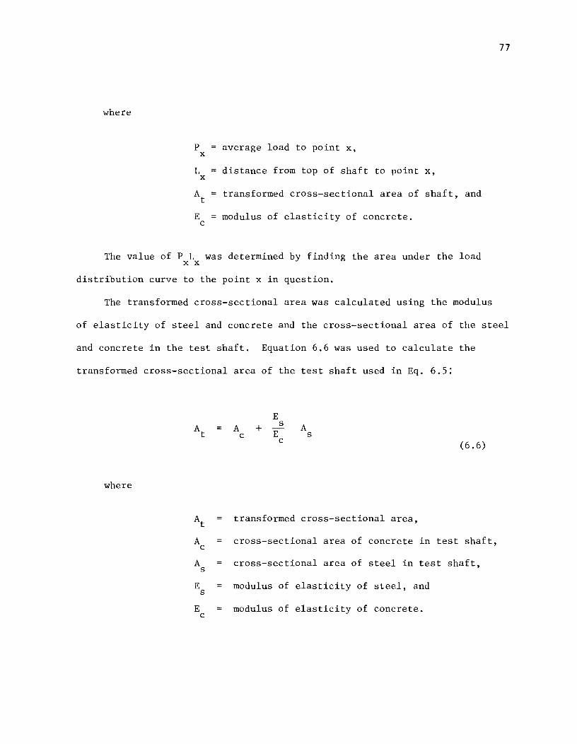
where

P average load to point x, x

L distance from top of shaft to point x, x

At transformed cross-sectional area of shaft, and

E modulus of elasticity of concrete. c

The value of P L was determined by finding the area under the load x x

distribution curve to the point x in question.

The transformed cross-sectional area was calculated using the modulus

77

of elasticity of steel and concrete and the cross-sectional area of the steel

and concrete in the test shaft. Equation 6.6 was used to calculate the

transformed cross-sectional area of the test shaft used in Eq. 6.5:

where

At

A c

A s

E s

E c

A + c

E s

E c

A s

(6.6)

transformed cross-sectional area,

cross-sectional area of concrete in test shaft,

cross-sectional area of steel in test shaft,

modulus of elasticity of steel, and

modulus of elasticity of concrete.

78

The modulus of elasticity of concrete was calculated froln the unconfined

compressive strength of concrete cylinders tested on the day of the load

lest. Equation 6.7 was used to calculate the modulus of elas::icity of

concrete (E ) that was used in Equations 6.5 and 6.6: c

where

E c

57 ,500~,' c

f' unconfined compressive strength of concrete. c

Analysis of Load Tests

(6.7)

The results of the analyses that were performed for each instrumented

load test are presented in the following pages. The results are presented

in graphical form with only a brief discussion. A more complete discussion

and comparison will be presented in a later section.

The results are presented separately for each of the instrumented tests

in the following order: the load-distribution curves, load transfer versus

shaft movement curves, and the unit end-bearing curves.

Test Shaft G-l. The load-distribution curves are plotted in Fig, 6.2.

The curves indicate that little load is being transferred to the soil

between the ground surface and 20 ft. At the maximum applied load of 495 tons

approximately 56 tons is being carried by the tip.

The curves of load-transfer versus shaft movement are srown in Fig. 6.3,

The curves indicate that the maximum load transfer occurs bet~'een 30 and 40 ft.

The curve of unit end-bearing versus tip movement is shewn in Fig. 6.4.

This curve indicates that the maximum bearing capacity of 4.4 tsf was achieved.

79

Load ,tons

10

0 [J

20 0 D

-.... .s::. 30 -0-CD Cl

40

50

60

Fig. 6.2 Load Distribution Curves, Test Shaft G-l

1.0

.80

..... ~ -------f/) -

..... 60 CD I ~~ ..... f/)

c 0

~ 7/ /' .... .-"0 .40 0 0 ~

.20 . . .. .-

o o .5 1.0

Movement tin. 1.5

Fig. 6.3 Load Transfer in Skin Friction vs Movement, Test Shaft G-l

Depth, ft.:

30-40 40-50

20-30

50-60

10-20

0-10

2.0

co o

81

Unit Bearing Capacity, tsf

o 1.0 2.0 3.0 4.0 5.0 o r-~~~~~r-Ir~r--r~r--r-,

.5 c: .. -c: G>

E 1.0 G> > 0 :E a. ~ 1.5

2.0

Fig. 6.4 Unit End Bearing Versus Tip ~ovement, Test Shaft G-1

82

Test Shaft G-3, Test 1. The load-distribution curves for this test are

shown in Fig. 6.5. The curves indicate that very little load was carried in

the top 40 ft. of the shaft, which was cased. At the maximum applied load of

209 tons approximately 28 tons was being carried by the tip.

Load-transfer versus shaft-movement curves are shown in Fig. 6.6. The

curves indicate that maximum load transfer has been developed at all

depths.

The plot of unit end-bearing versus tip movement is shown in Fig. 6.7.

The curve shows that the ultimate bearing capacity probably was achieved,

at the value of 3.9 tsf.

Test Shaft G-3, Test 2. Load-distribution curves for the second load

test on test shaft G-3 are shown in Fig. 6.8. The curves indicate that the

load transfer is fairly uniform from 40 to 60 ft and that grouting of the

top 40 ft. has definitely increased the load transfer in that region. At the

maximum applied load of 424 tons approximately 27 tons was carried by the tip.


curves also indicate that the load-transfer values are fairly ·:onstant from

40 to 60 ft. The curves also indicate that maximum values of Load transfer

were reached at all depths.

A plot showing the unit bearing capacity versus tip movement is shown in

Fig. 6.10. The curve indicates that an ultimate value probably was reached

and that it is 3.8 tsf.

Test Shaft G-4. The load distribution curves for this sh:lft are shown

in Fig. 6.11. The curves indicate that a negligible amount of load is carried

... .c -Co CD o

83

Load t tons

50 100 150 200 250

10

20

30

40

50

60

. 6.5 Load Distribution Curves, Test Shaft G-3. Test 1

84

1.0

.80

.... en -.. "- . 60 CD .... tn C 0 "-I-"0

.40 0 0 .J

.20

0 0 .5

Movement., in .

. 6.6 Load Transfer in Skin Friction versus Movement, Test Shaft G-3, Test 1

iDepth ,ft :

40-50

50-60

30-40

20-30 10-20 0-10

I.()

85


o 2.0 3.0 4.0 5.0 Or-~~~-.--'-~r--r--r-~--.--'

.5 c:

-c: Q)

E 1.0 Q)

> 0 ~

a. ~

1.5

2.0

Fig. 6.7 Unit End Bearing versus Tip Movement, Test Shaft G-3, Test 1

86

o o

10

20

-.... .. 30 .r:. -c. CD o

40

50

60

Load, tons

100 200 300 4()0

Fig. 6.8 Load Distribution Curves, Test Shaft G-3, Test 2

500

100,

.BOr-

't-

//~ en -... 60 .... G> 't-cn C c .... I- .40 rrrll "C ~ c 0 ...J

.20

o o .5

-

1.0 Movement tin .

1.5

Depth t ft :

50-60 40-50

"'" 30-40

20-30

10-20

0-10

2.0

. 6.9 Load Transfer in Skin Friction versus Movement, Test Shaft G-3, Test 2

00 -...j

68

c:: .. -c::

Q)

E Q)

> 0 ~

a. ...-

.5

1.0

1.5

2.0

Unit Bearing Capacity ,tsf

1.0 2.0 5.0 I

Fig. 6.10 Unit End Bearing versus Tip Novement, Test Shaft (-3, Test 2

89

Load, tons

o 50 100 150 o .-~----~~--~--~--~------~--~--~ 200 250

10

20

30

(/)

c: 0 -..

40 .s:::. -0-CI)

0

50

60

70

Fig. 6.11 Load Distribution Curves, iest Shaft G-4

90

in the top 40 ft of the shaft. At the maximum applied load of 225 tons

approximately 32 tons were being carried by the tip.


curves indicate that maximum values of load transfer were reached at all

depths. The curves show that the maximum load transfer occurred between

40 and 50 ft.

The plot of unit end bearing versus tip movement is shown in Fig. 6.13.

The curve shows that the ultimate bearing capacity was reached, at the value

of 10.2 tsf.

Load distribution curves for this shaft are shown in

Fig. 6.14. The curves indicate that the load transfer in the top 10 ft.

(0-10 ft.) and the bottom 10 ft. (50-60 ft.) is very small. The load

distribution curves also show that at the maximum applied load of 345 tons

approximately 99 tons were being carried by the tip.

The plots of load transfer versus shaft movement are shown in Fig. 6.15.

The load-transfer curves show that the maximum load transfer occurs between

20 and 30 ft. The curves also indicate that maximum load transfer has been

developed at all depths.

Unit end-bearing versus tip movement is shown in Fig. 6.16. The curve

indicates that the ultimate bearing capacity was achieved at th~ value of

14.0 tsf.

Shaft E-2. Load-distribution curves for this shaft ace shown in

Fig. 6.17. The curves indicate that very little load is being transferred in the

top 20 ft. of the shaft. The load-distribution curves also show that the maxi

mum applied load of 865 tons approximately 420 tons were carried by the tip.

1.20

1.00

.... 0.80 (/) -L-

a.> .... (/)

c 0.60 0 L-

I-

"'0 0 0

-.J 0.40

0.20

o o

91

Depth, ft :

.10 .20 .30 .40

Movement, In.

Fig. 6.12 Load Transfer in Skin Friction versus Movement, Test Shaft G-4

40- 50

50- 60 60-70

70-80

0-40

.50


° ~ 2 jO 4 jO GiO 8 iO I °1.0 I~.o

0.1

c -C 0.2 CD

E CD > 0 ~

a. 0.3 ~

0.4

05 L Fig. 6.13 Unit End Bearing versus Tip Hovement, Test Shaft G-4

0.0 N

-.... .. .c -Q. G> 0

o o

10

20

30

40

50

60

Load, tons

100 200 300 400

0

. 6.14 Load Distribution Curves, Test Sha~t E-l

93

..... ", -

1.0

O.S

Q; 0.6 ..... ", c: c .= -g 0.4 o

...J

0.2

o o no ,..

v . .:::. '" A U.Cot 0.6

Movement fin .

0.8

Dept h , f t :

20-30

30-40

10-20

40-50

50-60 o -10

1.0

• 6.15 Load Transfer in Skin Friction versus Hovement, Test Shaft E-1

\0 po

Un i t Be 0 r i n 9 Co pO cit y, t sf

o 4.0 8.0 12.0 16.0 O~~=--.-------.-------.-------.

.2

c:

..: .4 c: Q)

E Q)

> o :E a. .6 I-

.8

1.0

Fig. 6.16 Unit End Bearing versus Tip ~~vement, Test Shaft E-1

95

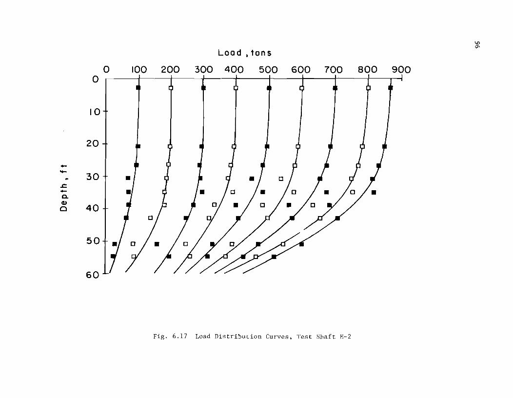
o

10

20

-- 30 .s:::. -a. CIJ Q 40

50

60

Load, tons

o 100 200 300 400 500 600 700

Fig. 6.17 Load Distribution Curves, Test Shaft E-2

800 900

\0 0"

97

Load transfer versus shaft-movement curves are shown in Fig. 6.18. The

curves in Fig. 6.18 indicate that maximum load transfer was developed at all

depths with the maximum load transfer occurring between 51 and 60 ft.

Unit end bearing versus tip movement is shown in Fig. 6.19. The curve

shows that substantially all of the end bearing had been developed and that

the maximum value was 59.5 tsf.

Discussion of Load Tests

Discussions of the results from testing shafts G-1, G-3, G-4, E-1, and

E-2 will be presented first because these shafts were instrumented. The dis

cussions concern tip resistance in clay, tip resistance in sand, side resis

tance in clay, side resistance in sand, and the influence of construction

procedures. The discussion of the load test of shaft G-2 will be given in

the section on construction procedures.

The principal thrust of the research reported in this report was to in

vestigate the effect of leaving the casing in place when the construction

plan called for removing the casing. Prior to discussing the results of the

research study related to that topic, it is desirable to discuss the specifics

of load transfer from drilled shafts to the supporting soil, as noted above.

Results pertaining to the effects of leaving casing in place and of the

grouting of the casing will be discussed in the section on the influence of

construction procedures.

Tip Resistance in Clay. There were three instrumented test shafts that

had their tips in clay. These were test shafts G-1, G-3, and G-4. As men-

98

..... V> -.. 'Q) ..... V> c:

2.0

1.5

o 1.0

Depth, ft :

51 - 60

43-51

~ 31 -43 '"0 o o -.J

0.5

o o 0.5

~ ____ ---- 21 - 31

1.0

Movement, In.

I 1.5

0-21

Fig. 6.18 Load Transfer in Skin Friction Versus Movement, Test Shaft E-2

Ultimate Base Resistance, tsf

o ~ 10 20 30 40 50 60

c: ·-".50 -c: CD E CD > o

::E a. 1.0 I-

1.5

Fig. 6.19 Unit End Bearing versus Tip Movement, Test Shaft E-2

\0 \0

100

tioned earlier, the ultimate unit bearing capacities for the shafts were

4.4 tsf for shaft G-1, 3.9 and 3.8 tsf for the two tests of shaft G-3, and

10.2 tsf for shaft G-4.

A plot of the unit end bearing versus tip movement for Site 1 is shown

in Fig. 6.20. Test shafts G-1 and G-3 were used to develop this plot

because the tips for both shafts were at a depth of 60 ft. The results from

the three test loadings are plotted, along with an average curve.

Theoretical bearing capacity values were calculated using Equation 6.8.

where

N s c u

(6.8)

N bearing capacity factor (assumed to have a value of 9.0), c

qb unit base resistance, and

Su undrained shear strength.

It is of interest to note that the use of Eq. 6.8 yielded a value of

3.6 tsf for test site 1 and a value of 8.6 tsf for test site 2.

The downward movement necessary to develop full end bearj_ng ranged

from about 3 to 5% of the diameter of the base at test site 1 and was 2%

of the diameter of the base at test site 2.

101

Unit Bearing Capacity t tsf

1.0 2.0 3.0 4.0 5.0

.5 .

c:

-c: 1.0 (J)

E Average Q)

> 0

::E G-3 0-

1.5 Test 2 ~

2.0

Fig. 6.20 Unit End Bearing versus Tip Hovement for Clay

l02

Tip Resistance in Sand. Only two test shafts had their tips in sand.

These were test shafts E-l and E-2. As mentioned in an earlier section,

the ultimate unit bearing capacity for shafts E-l and E-2 were 14.0 tsf

and 59.5 tsf respectively. Considering that the shafts were both at the same

depth, 60 ft, and were approximately 10 ft apart, the difference in the

ultimate unit bearing capacities would seem quite large. A possible ex

planation of the difference would be that test shaft E-2 is resting on the

layer of limestone that was mentioned in Chapter 4. The limestone was

excavated in the construction of test shaft E-l, whereas there was none

excavated in the construction of test shaft E-2. By making the above

explanation for the differences in bearing capacity, it is assumed that the

ultimate bearing capacity of test shaft E-l would be what would normally be ex

pected for the sand at the test site.

Table 6.1 presents a tabulation of some computed values of unit bearing

capacity along with a reference and a brief description of the method of

computation. It should be noted that methods of computed bearing capacity

of the tips of driven piles are included in Table 6.1. Such methods are

included because, in the construction of both test shafts, a steel casing was

driven with a vibratory hammer to a depth of 60 ft, therefore, there should

be some correspondence between the behavior of the tips of the test shafts

and the tips of driven piles.

Reference

TABLE 6.1 TABULATION OF THEORETICAL VALUES OF BEARING CAPACITY IN SAND

(Depth = 60 ft., Diameter = 3 ft., tP = 300

)

Brief Description of Method

Calculated Unit Bearing Capacity, tsf

Quiros and Reese (1977) q = qb/K; for u

9

Reese and Wright (1977)

API (1980)

1.0 inch of movement

Design graph; at settlement of O.OSB

q = P N ; for u 0 q

driven and/or bored piles

13

8

Coyle and Castello (1981) Design graph, for driven piles

38

Meyerhof (1976)

Meyerhof (1976)

where

q 1.2N; for bored u

piles

q = 4N for driven 11 '

piles

q. unit bearing capacity, u

19

64

qb base capacity at 5 percent tip movement,

K reduction factor,

B diameter of base,

P = effective overburden pressure, o

N bearing capacity factor, and q

N average standard penetration blow count.

103

104

Side Resistance in Sand. Only test shafts G-l and E-2 ~ill be discussed

in this section on side resistance in sand. The other tests will be discussed

in a later section of this chapter dealing with the influence of construction

methods.

Test shaft G-l was constructed at test site 1 in Galveston. Approxi

mately the top 40 ft of the shaft was in sand. The shaft failed at an axial

load of 495 tons with 270 tons carried in skin friction by the sand. Refer

ing to Fig. 6.3, it can be seen that the maximum load transfer in skin

friction occurred at a downward movement of approximately 3.6Z of the shaft

diameter. The amount of skin friction that was measured was~igher than

what was expected, based on past tests. It is believed that the large

amount of load transferred developed was due to the high slum) (9-1/2 to 10 in)

of the concrete. Having a high slump concrete enabled the co~crete to dis

place the slurry in the excavation more efficiently and to flow outward

easily and produce a better soil-concrete contact when the casing was

removed.

Table 6.2 shows a comparison of theoretical values of skin friction for

test site 1, as computed from different criteria. Shown in Fig. 6.21 is a

plot of the ultimate load transfer versus depth for each of the measured

values. Values of load transfer were calculated for 5 ft intervals and

straight lines were used to approximate the values between the computed

points. As can be seen in Table 6.2, the method of O'Neill and Reese (1978)

Reference

Meyerhof (1976)

Meyerhof (1976)



Reese and Quiros (1977)

Reese and Touma (1972)

O'Neill and Reese (1978)

O'Neill and Reese (1978)

Unpublished

TABLE 6.2 TABULATION OF THEORETICAL VALUES FOR SKIN FRICTION OF DRILLED SHAFTS IN SAND

(Test Site 1, 48-in. shaft, 40 ft in sand)

Brief Description Theoretical Ultimate of Criteria Skin Friction, tons.

f = Kptan¢ 141 s

K taken from graph

f NI100 110 s

f Rptan¢ 163 s

K 0.7

f N for N 53 317 = - < s 34

f N-53 s 450 + 1.6

for 53 < N < 100

f .026 N 330 s

f aptan¢ 149 s

a is a function of depth

f Sp 381 s

S is a function of £/d

f 1\ P 259 s c

tan( ¢ - 5) t < 12 Sc for -

d

f K P tan ¢ 314 s c c

Kc = l.0

105

Notation On Graph

1

2

3

4

5

6

7

8

9

(continued)

106

TABLE 6.2. (Continued)

where

f ultimate skin friction in tsf, s

K lateral earth pressure coefficient,

p effective overburden pressure of soil, tsf,

o effective angle of friction,

N average standard penetration test blow count,

a lateral pressure coefficient,

B factor relating load transfer to in-situ vertical

soil pressure,

Bc factor relating load transfer to in-situ

vertical concrete pressure,

P effective overburden pressure of concrete, tsf, and c

K lateral concrete pressure coefficient. c

-..... .s:::.

o

10

Q. 20 Q)

c

30

40

o Ultimate Load Transfer, ts f

0-1 ~- 6

181-2 .-7

0-3 .-8 'V - 4 0-9

"'- ' .......

~ • - 5 0- Measured

"'~" .... ~ ~"C::~~:- :-:"::::: _ _ _ _ _

~. 0_______. ~" ........... _._.._,. -;::-v ", -~"----- ~-'W, \ ,_ ....... ~ _ . .~ .. "'-,-\ ....... -b-'

.. . ... /)v 1 .~ , . I/" '\

i /' / '. I V <0' •

~"

\ "'""" ~~/ .. /"'/\ l I

/ ............. I!r" _ L: __ 0 ___ 0 . .. - -I ....

/-/------ I .... ········· .. · 8'- - - - • · .. ·li .. · r.

Fig. 6.21 Theoretical and }~asured Unit Skin Friction in Sand, Test Site 1 I-" o -...J

108

yields an ultimate skin friction load of 259 tons. which is v=.ry close to the

measured value of 270 tons. Other methods that also predict 'Jalues that are

fairly close are Reese and Wright (1977). 317 tons and the unpublished

criteria. 214 tons. It should be noted that two of the three methods that

gave reasonable values. O'Neill and Reese (1978) and the unpuhlished criteria.

assume that the load transfer is to be interpreted as being controlled by

the lateral fluid pressure from the concrete.

Test shaft E-2 was constructed at test site 3. The shaft: was com

pletely embedded in sand. Shaft E-2 failed at an axial load of 865 tons

with 445 tons carried in skin friction. Referring to Fig. 6.18. it

can be seen that the maximum load transfer in skin friction occurred at a

downward movement of approximately 4.0% of the shaft diameter. Again, the

amount of skin friction that was measured was higher than what was expected.

based on past tests. As mentioned before, it is believed that the large

amount of skin friction developed was due to the high slump concrete.

Table 6.3 shows a comparison of theoretical values of skin friction for

test site 3 as computed from different criteria. Shown in 6.22 is a

plot of the ultimate load transfer versus depth for each of the methods in

Table 6.3 and for the measured value. As can be seen in Table 6.3, the

unpublished criteria computes an ultimate skin friction load of 429 tons.

which is comparable to the measured value of 445 tons. Again it is of

interest to note that the theoretical method that best predicted the

ultimate load in skin friction was one that assumed the load transfer was

controlled by the lateral fluid pressure of the concrete.

TABLE 6.3 TABULATION OF THEORETICAL VALUES FOR SKIN FRICTION OF DRILLED SHAFTS IN SAND

(Test Site 3, 36" x 60 ft)

Reference Brief Description Theoretical Ultimate of Criteria Skin Friction, tons.

Meyerhof (1976) Kptan ¢ 64

K taken from graph

Meyerhof (1976) = N/100 64

Reese and Wright (1977) f Kptan ¢ 228

s K 0.7

Reese and N Wright (1977) 34 for N< 53 187

= N-53 + 1.6 450

Reese and for 53<N<100

Quiros (1977) 0.026N 165

Reese and Touma (1972) = aptan ~ 183

a is a function of depth

O'Neill and Reese (1978) SP 524

e is function of £/d

O'Neill and Reese (1978) =s p 241

c ('

Sc tan <<P- 5) for Q, /d<12

tan (~ -17) for 12 <~ < 23 d

Unpublished K p tancjl 438 c c

109

Notation on Graph

1

2

3

4

5

6

7

8

9

--Ultimate Load Transfei, tsf ,..... 0

00 0.2 0.4 0.6 0.8 1.0 1.2 1.4 1.6

~~_. '"JII 0 I 8. 6 f., "-";'-_ ,/ ~ 0 2 "'V 7

I 0 k1~~ , " .. 3 <> 8 .,; \. "- '" .....

I ~( • ....,~',.. ~ • 4 • 9

" """ '--, ..... l1li 5 0 M easu red 20 1-<bI ~A ~, --'" ~

" " "-

:: l:to """ ~ \ ~"

~ 30 ~ ~ '''-''<''''-''' "

~ ~ ',- "'-." '~ 401- '

+ : \: "',

~ ~ ~ 4~ -"., ~ -t ~ ".\ '\

50~ ~ ~ ~ ~ '~,\ K ". ~ "..,

~ b " "~ .. ~~ ~I

60 L- "0 \ 1!Q.,,~ ~ \ ,.~I

. 6.22 Theoretical and l~asured Unit Skin Friction in Sand

III

In general there are two methods that are used to calculate theoretical

values of load transfer in sand, the first method determines load transfer

by using equations of the form

where

f s

K

Kptan 0

lateral pressure coefficient for earth (K for c

concrete),

(6.9)

p overburden pressure for earth (p for concrete), and c

o angle of friction of soil.

In this method values of p are computed, 0 is estimated or determined by

correlation with N-Values, and values of K are usually in the

particular method.

The other method used to calculate load transfer is one that computes

the load transfer from results of the Standard Penetration Test (SPT).

This method is of the form

where f

s x N

x = correlation factor, and

N = blow count from SPT.

(6.10)

In Tables 6.4 and 6.5 are comparisons of theoretical and measured values

of K and x for test site 1 and test site 3, respectively. The measured

values of K and x were calculated using the values of load transfer that

were determined from results of the load tests. As may be seen in the tables,

several methods for design of drilled shafts were investigated.

Referring to Figs. 6.21 and 6.22 and to Tables 6.2 and 6.3, it is

TABLE 6.4 COMPARISON OF MEASURED AND THEORETICAL VALUES OF K AND x FOR TEST SITE 1

Depth, Measured Unpublished Measured Meyerhof Reese & Reese & Measured Meyerhof Reese & Reese & Ft (1976) Wright Touma (1976) Wright Quiros

(1977) (1972) (1977) (1977) K K K K K a x x x x

c c

5 1. 28 1.0 1.72 0.2 0.7 0.7 .028 .01 .029 .026

10 1. 30 1.0 1. 75 0.2 0.7 0.7 .079 .01 .029 .026

15 1.15 1.0 1. 55 0.2 0.7 0.7 .036 .01 .029 .026

20 1.06 1.0 1. 43 0.2 0.7 0.7 .051 .01 .029 .026

25 .79 1.0 1.06 0.8 0.7 0.7 .017 .01 .029 .026

30 .70 1.0 .94 0.9 0.7 0.6 .014 .01 .028 .026

35 .72 1.0 .973 0.8 0.7 0.6 .022 .01 .029 .026

40 .75 1.0 1.01 0.2 0.7 0.6 .050 .01 .029 .026

......

...... N

TABLE 6.5 COMPARISON OF MEASURED AND THEORETICAL VALUES OF K AND x FOR TEST SITE 3

Depth, Measured Unpublished Measured Meyerhof Reese & Reese & Mea~ured Meyerhof Reese & Ft (1976) Wright Touma (1976) Wright

(1977) (1972) (1977)

K K K K K a x x x c c

5 .24 1.0 .32 0.2 0.7 0.7 .002 .01 .029

10 .26 1.0 .35 0.2 0.7 0.7 .007 .01 .029

15 .34 1.0 .46 0.2 0.7 0.7 .021 .01 .029

20 .39 1.0 .53 0.2 0.7 0.7 .027 .01 .029

25 .50 1.0 .68 0.2 0.7 0.7 .034 .01 .029

30 .74 1.0 1.00 0.2 0.7 0.6 .042 .01 .029

35 .70 1.0 .94 0.2 0.7 0.6 .043 .01 .029

40 1.15 1.0 1. 54 0.2 0.7 0.6 .093 .01 .029

45 1.30 1.0 1. 76 0.2 0.7 0.5 .129 .01 .029

50 1.27 1.0 1. 50 0.2 0.7 0.5 .128 .01 .029

5) 1.32 1.0 1. 78 0.2 0.7 0,5 1.19 .01 . )29

----~---"' -----'"

Reese & Quiros (1977)

x

.026

.026

.026

.026

.026

.026

.026

.026

.026

.026

. ;:126 ...... ...... w

114

obvious that theories that use SPT values to determine skin friction in sand

do not work well for test sites 1 and 3. Theories that use lateral earth

pressure K all seem to give lower values of skin friction than what was

measured, indicating that possibly the value that is used for K should be

increased.

The unpublished theoretical method that uses the latera~ pressure of

fluid concrete K seems to be the best method for calculating values of skin c

friction at test sites 1 and 3. This method calculated a higher value of

total skin friction at site 1 by 44 tons and a lower value of total skin

friction at site 3 by 7 tons.

Side Resistance in Clay. There were only two instrumented test shafts,

constructed without casings, that had any portion of the shaft in clay.

These were test shafts G-l constructed at test site 1, and G-4 constructed

at test site 2. Test shaft G-l was embedded in clay from 40 to 60 ft, and

test shaft G-4 was embedded in clay from 40 to 80 ft.

Test shaft G-l failed at an axial load of 495 tons of wtich 169 tons

was skin friction in the clay. Referring to Fig. 6.3, it can be seen that

the maximum load transfer in skin friction occurred at a downward movement

of approximately 3.6% of the shaft diameter. Test shaft G-4 failed at an

axial load of 225 tons of which 175 tons was skin friction in the clay.

Referring to Fig. 6.12 it can be seen that the maximum load transfer in skin

friction occurred at a downward movement ranging from 0.7 to 1.9% of the

shaft diameter.

115

Theoretical values of unit skin friction in clay are calculated using

6.11 from Reese and Quiros (1977):

f s

a s u

(6.11)

where

f unit skin friction, tsf, s

a correlation factor, and

s undrained shear strength, tsf. u

Quiros and Reese recommend that a value of 0.6 he used for a.

A plot is shown in Fig. 6.23 of the maximum load transfer versus depth

for the portions of test shafts G-1 and G-4 that are in clay. Also shown in

this plot is a theoretical curve of load transfer that was calculated using

Equation 6.11. Values of shear strength from unconfined compression tests

and unconsolidated-undrained triaxial tests from both sites were combined and

were used in determining values of s at the depths where data points are u

shown in Fig. 6.23. It was assumed that the properties of the soil at both

sites were identical, because the two sites are only 700 feet apart. The

profiles of soil properties confirm the above assumption. Load-transfer

values were calculated only at depths indicated by data points.

-..... ~

Ultimate Load Transfer, tsf

o 0.2 0.4 0.6 0.8 1.0 1.2 40 ~I ------~------~------~------~------~------~

~ r Theoretical

50 ~ \

~

Q. 60 f CD o I

~ , 70 4 ,

l

80

Fig. 6.23 Theoretical and Measured Unit Skin Friction in Clay, Test Sites 1 and 2

I-' I-' (J'\

117

Referring to Fig. 6.23, it can be seen that the theoretical method of

computing load transfer did not work very well. The plot of load transfer

versus depth for test shaft G-4 seems quite erratic, but the scatter is due

principally to the way the load-distribution curves were drawn, with straight

lines instead of a smooth curve.

Table 6.6 shows a comparison of measured and theoretical values of a

for test shafts G-l and G-4. The measured value of a was determined in the

following manner:

1. The measured side resistance at the desired depth was obtained

from the load distribution curves.

2. The average shear strength at the desired depth was obtained

by averaging shear strength values from unconfined compression

tests and unconsolidated-undrained triaxial tests from 5 ft

above and below the desired depth.

3. The value of a was computed by Eq. 6.11.

As was expected the measured values of a were much greater than the

theoretical value of 0.6. It is of interest to note that other investigations

have reported a values generally ranging from 0.25 to 0.7; however, in some

cases values greater than 1.0 have been reported. The "actual" value of a

should not exceed 1.0 because this means that the load transfer is equal to

the in-situ shear strength of the soil, which should be the maximum load

transfer possible. However, values of a greater than 1.0 can be calculated

from load tests if conventional laboratory tests underestimate the in-situ

strength of the soil, which is entirely possible.

l18

TABLE 6.6 COMPARISON OF MEASURED AND THEORETICAL VALUES OF Q:

Depth. Undrained shear Theoretical Shaft G-l Shaft G-4

Ft. strength, tsf a Measured ct Measured ct

45 0.275 0.6 2.89 2.85

50 0.406 0.6 1.50 1.58

55 0.456 0.6 1.22 1. 97

60 0.375 0.6 3.04

65 0.344 0.6 2.21

70 0.369 0.6 1. 27

75 0.425 0.6 0.89

119

Influence of Construction Methods

In the load tests that are discussed in this report there are three

influences of construction that can be discussed. These are: (1) the

influence of a steel casing on the load-carrying capacity when the casing is

put in an over-drilled hole; (2) the influence of a driven steel casing on

the load capacity; (3) the influence of the concrete's flow qualities.

The influence of a steel casing on the load capacity when the casing was

put in an over-drilled hole was investigated at test site 1. As mentioned

before, there were three test shafts at this site, G-1, G-2, and G-3, with

shafts G-2 and G-3 having casings extending part of or for the full length of

the shaft. As expected, when shafts G-2 and G-3 were first tested, they

failed at relatively low axial loads. tVhen the second load tests were done

on shafts G-2 and G-3, after grouting, the axial loads at failure increased

significantly.

Since test shafts G-1 and G-3 were both instrumented, a comparison of

measured values of the ultimate load transfer can be made. This comparison

was made in Fig. 6.24 where a plot is given of the maximum load transfer

versus depth. The results from the three test loadings are plotted. This

plot shows ,that the grouting was effective in increasing the load transfer

in the grouted region 0 to 40 ft of test shaft G-3.

Due to the large quantity of grout that was used, 8 cu yd , another

computation of the load transfer was made assuming that there was a uniform

increase in diameter over the grouted zone. A new diameter of 3.98 ft was

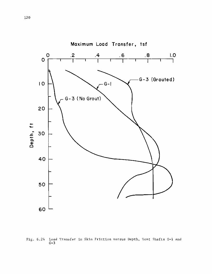
120

-.....

o

10

20

.d 30 -Q.

CD CI

40

50

60

Maximum Load Transfer, tsf

o .2 .4 .6 .8 1.0

G-3 {Grouted)

Fig. 6.24 Load Transfer in Skin Friction versus Depth, Test Shafts G-l and G-3

Ul

calculated for the top 40 ft of the shaft. Maximum values of load transfer

determined using a diameter of 3.98 ft are 25% less than the maximum values

determined using a 3.00-ft diameter.

Test shaft G-2 was not an instrumented shaft so only the load-settlement

curves are available. The unit end bearing was estimated as 4 tsf, yielding

a load on the tip of 28 tons.

In the first load test of test shaft 2 the maximum applied load was

89 tons. Thus, it is estimated that 61 tons were carried in skin friction.

Assu~ing that there is no load transfer in the top 10 ft, an average 10ad

~ransfer value of 0.12 tsf can be computed. The value of 0.12 tsf seems

reasonable in comparison with the maximum load-transfer curve in Fig. 6.24

for the top 40 ft of the 36-in.-diameter shaft without grout.

In the second load test of test shaft 2, after grouting the lower 15 ft

the maximum applied load was 373 tons. Subtracting the computed end bearing

of 28 tons leaves 345 tons carried in skin friction. Using the previous 10ad

transfer value of 0.12 tsf for the top 50 ft of the shaft, where no grouting

was done, yields a total load of 45 tons. This leaves 300 tons of load

carried in skin friction in the grouted area, which gives a load-transfer

value of 2.1 tsf.

This value of 2.1 tsf seems quite large, even after grouting. Consider

ing the large amount of grout used, 6 cu yd, it is possible that grouting

caused a larger effective diameter. Assuming that there was a uniform in

crease in diameter over the grouted zone, a new diameter was calculated for

the lower 15 ft of the shaft. Using this diameter of 4.77 f~ a new value

122

for the load carried in end bearing was determined to be 71 tons. Subtracting

the end bearing and the 45 tons carried in skin friction in the top 50 ft,

leaves 257 tons of load carried by the grouted area. A load-transfer value

for the lower 15 ft of 1.1 tsf was then computed. The value ·)f 1.1 tsf

seems much more reasonable in comparison to values shown in Fi s. 6.24.

The influence of a driven steel casing on the load capacity was investi

gated at test site 3. As mentioned before, there were two inst::umented test

shafts at this site, E-l and E-2. Test shaft E-l had a casing extending the

complete length of the shaft. Test shaft E-2 had no casing. The results of

the analyses of readings from the l'lustran cells showed that teBt shaft E-I

carried a total load of 246 tons in skin friction while test shaft E-2 aarried

445 tons in skin friction. A comparison of the maxinum load transfer values

for t~1e two shafts was done and is shown in Fig. 6.25. This t shows that

in the upper portion that the load transfer is higher for test shaft E-I, but

overall the load transfer is greater for shaft E-2.

Test shaft E-l was then analyzed as a driven pile. Table 6.7 shows a

comparison of theoretical values of skin friction, for driven piles, using

different methods. Shown in Fig. 6.26 is a plot of the ultimate load trans-

fer versus depth for each of the methods in Table 6.7 and for the measured

values. As can be seen in Table 6.7 and Fig. 6.26, the method suggested by

Meyerhof (1976) gives the best results.

The fact is well known that the flow characteristics of concrete (slump)

have an important bearing on the quality of drilled shafts. There have been

a number of instances where drilled shafts have been excavated ana found to

be structurally unsound because concrete has failed to flow through rebar cages


o 0.2 0.4 0.6 0.8 1.0 1.2 1.4 1.6 01 I I I I 1 I

10 I \ ~

E-I

I "\ ~ 20

-.... .. -= 30 c. CD

0

40

50 I

x b 1.91 ...

60

Fig. 6.25 Load Transfer in Skin Friction versus Depth for Test Shafts E-1 and E-2 t-' IV W

124

Reference

TABLE 6.7 TABULATION OF THEORETICAL VALUES FOR SKIN FRICTION OF DRIVEN PILES IN SAND

(Te: Site 3, 48-in shaf t by 60 f t long)

Brief Description of Criteria

Theoretical Ultimate Skin Friction, tons

Meyerhof (1976) f s

N/SO 128

Meyerhof (1976)

Coyle & Castello (1981)

where

f '" Kptan <p s

K taken from graph

Taken from design graph

f ultimate unit skin friction, s

260

71

K coefficient of lateral earth pressure,

p = effective overburden pressure, and

¢ effective angle of friction.

Notation on Graph

1

2

3

125

Ultimate Load Transfer, ts f

00 1.0

01 o 2

~ I

83 10

• Measured I .. I

~ ~ \ \

\ 20 0 \

\ \

~ - Q -.- , , ,

~ .r:.

30 Q -0. CD \

\ Q

9> I

I

~ 40 ¢

~ 50 ~

"0 ""

60 "0

7ig. 6.26 Theoretical and }leasured Load -:;:,ransfer, Test Shaft E--l

126

or has failed to displace slurry completely in the excavation.

There are little data, however, on the degree to which the slump of con

crete affects load transfer in skin friction. As mentioned in Chapter 4,

when test shaft G-4 was constructed- the concrete had a low slump when it

arrived on the job site, water was then added to increase the slump, but by

the time the pour was complete the slump was again low. Data from the Mustran

cells revealed virtually no load transfer in the 40-ft thick surface stratum

of sand. The load test of test shaft G-4 was only a short distance from test

shaft G-l making a comparison possible. The comparison of the maximum load

transfer versus depth for test shafts G-l and G-4 is shown in Fig. 6.27. The

difference in load transfer in skin friction in the sand is striking.

Had the unit load transfer in the G-4 shaft in the sand been equal to

the value obtained from the G-l shaft, a load of 157 tons would have been

carried in the sand by shaft G-4. The experience suggests the desirability

of using a concrete that acts almost like a liquid and the pOf;sibility of

basing computations of axial load in sand on stresses in the fresh concrete

rather than on overburden stresses in the soil.

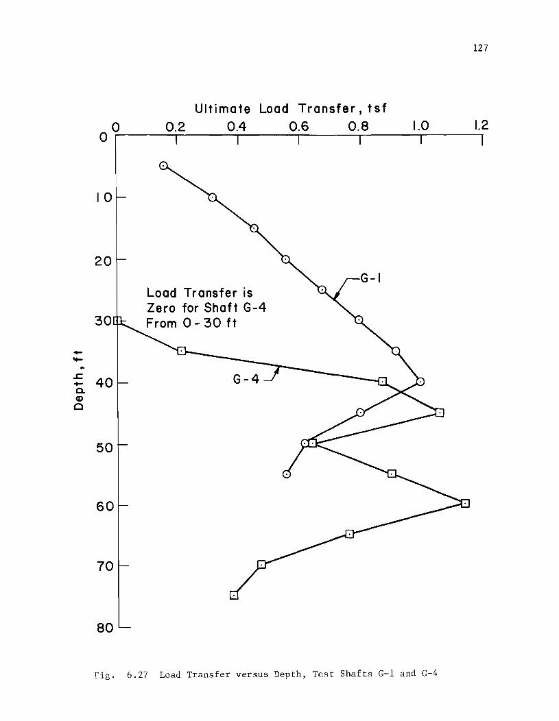
127


0°r-__ ~0,.2 _____ 0~.~4 ____ ~0~.6~ ___ 0~.~8 ____ ~1~.0~ __ ~1.2

10

20

Load Transfer is Zero for Shaft G-4

30 From 0 - 30 ft

-~ .. .t:.

40 G-4 -a. G)

0

50

60

70

80

Fig. 6.27 Load Transfer versus Depth, Test Shafts G-l and G-4

CHAPTER 7. SUGGESTIONS CONCERNING CONSTRUCTION METHODS

Due to the results of the investigation of the influence of construction

procedures, the following suggestions are made concerning construction methods.

First, it has been shown that when a casing has to be left in place, the load

capacity of the shaft is greatly reduced. This was true whether the casing

was driven or placed in an over-drilled hole. Therefore, some type of remedial

measure must be taken.

A remedial measure that can be taken is grouting around the shaft if the

casing was placed in an over-drilled hole. This was done at test site 1 and

proved to be quite successful. It should be noted that these were the only

tests of this sort that have been performed; therefore, grouting cannot be

considered a proven method of increasing the load capacity. If grouting is

the remedial measure that is chosen, then some technique should be used to

prove the load capacity of the shaft. A method has been developed and used

in Europe for some time that can be effective. It is called the TNO method,

after the firm in the Netherlands that did the development.

Robert Arias (1977) reported that the Institute TNO for Building Materials

and Building Structures, a Netherland organization for applied scientific

research, has developed a method of dynamic pile testing. The TNO organization

claims the test will provide information regarding load-carrying capacity,

skin friction, and static deformation.

U9

130

A schematic of the testing arrangement is shown in Fig. 7.1. The top

of a shaft is prepared with a layer of epoxy to which a steel plate is

fastened. In addition to being held by epoxy, the plate is held by bolts

that are fastened into the concrete. An electronic load cell is bolted to

the steel plate. The shaft or pile is stressed by a blow from a small drop

hanuner (approximately 880 lbs.). An electronic theodolite kE.eps track of

the movements at the top of the shaft to obtain a time-displacement curve.

The data recorded are analyzed by use of a proprietary computET program and

the results from the computations allow a load-settlement curve to be plotted.

TNO claims that the force-displacement curve obtained can be analyzed to

obtain the load carried in skin friction.

Actually, the TNO method is just a variation of the wavE-equation method

of analysis of pile foundations. That method has had extensive development

in the United States, principally by researchers at Texas A & M University

and at Case Institute. The wave-equation method can readily be extended to

drilled shafts.

Other remedial measures that can be taken are to add one or more drilled

shafts, next to the drilled shaft with the casing, to compensate for the

reduced capacity of the original shaft. This type of remedial measure would

probably be done if the steel casing were driven because there would then be

no annular space to grout.

Another suggestion related to the research that was performed has to do

with the flow characteristics of concrete. From the tests that were performed,

there seems to be evidence to indicate that increasing the liquidity of fresh

Light Source

Drop Hommer

~ Steel. Plate ~ - Epoxlte

-----lack Plate for Measurement of Movements

Pile

(After Arias 1977)

Electronic Theodolite

Graphical Presentation of LoadDisplacement Curve

Digital Conve rter Mini Computer

Force

~ Displacement

Fig. 7.1 Schematic of 7~m :;:'esting Arrangement

I-' W I-'

132

CQncrete (increasing the slump) increases the load transfer in skin friction.

With additives that can be put in concrete, slumps of 9 to 10 inches will

yield concrete of appropriate strength and apparently will yield larger

values of load transfer in skin friction. Additional research is needed to

confirm this tentative conclusion.

The studies that were performed indicate that the leaving of casing in

place should be avoided if at all possible. Appendix D presents a discussion

of some cases where it would be difficult to retrieve a casing.

CHAPTER 8. CONCLUSIONS AND RECOMMENDATIONS

This study has been concerned with the influence of construction

procedures on the load carrying capacity of drilled shafts. In the study

drilled shafts with casings left in place were compared to drilled shafts

with no casings. Also, a drilled shaft constructed with concrete of bad flow

characteristics was compared to one constructed with concrete of good flow

characteristics. Six full-scale test shafts were constructed by the casing

method, five of which were instrumented with Mustran cells. In the analysis

of these tests, the results were not only compared to each other, as men

tioned above, but were also compared with recommended design procedures. In

the following sections the main conclusions and recommendations concerning

the construction, design, and instrumentation of drilled shafts will be

summarized.

Conclusions

1. Leaving casing in place when the excavation has been over-drilled

dramatically reduced the capacity of a drilled shaft.

2. The grouting of the annular space between the casing and the exca

vation caused a significant increase in capacity for these tests.

3. Leaving the casing in place when the casing has been driven in sand

dramatically reduced the capacity of a drilled shaft.

4. There is evidence to indicate that increasing the liquidity of fresh

concrete (increasing its slump) increases the load transfer in skin friction.

D3

134

5. The load transfer in skin friction was a nonlinear function of the

downward movement of a drilled shaft.

6. The maximum load transfer in skin friction occurred at a small

downward movement of a drilled shaft.

7. The maximum load transfer in skin friction for sand increased with

depth with almost a linear function.

8. The maximum end bearing in clay agreed well with bearing capacity

theory and required more downward movement than did the maximJm skin friction.

9. The present design procedures for drilled shafts in sand tend to

underestimate the load carried in skin friction.

10. Design procedures that use standard penetration blow counts greatly

underestimated loads carried in skin friction.

11. The unpublished design equation (f = K P tan0) wa,s the best oversec

all method of predicting the measured loads in skin friction for sand.

12. A value of a 0.6 has been recommended for design of drilled shafts

in clay. A value for a of more than 1.0 was obtained from the limited data

from the load tests reported herein.

13. The Nustran-cell instrumentation system provided an adequate method

of the measurement of axial loads in a drilled shaft.

Recommendations

1. When a casing has to be left in place, some type of remedial

measure should be taken to insure the integrity of the fo~ndation.

2. Grouting of the annular space is recoffil-uended as a remedial measure

when the casing is left in an over-drilled hole.

135

3. Any type of remedial measure that is taken should be verified by

use of some type of load test.

4. When fluid concrete (slump 9 tolD in.) is used in constructing

drilled shafts in sand, the following design equation can be used to predict

the side resistance:

where f

s K P tan0

c c

f ultimate unit skin friction, s

K lateral pressure of concrete, c

Pc effective overburden pressure of concrete, and

o effective angle of internal friction of soil.

5. Internal instrumentation for the measurement of the distribution of

axial load with depth should be employed in any future test shafts. Experience

has shown that extreme care must be used in the installation and operation of

any of the available systems (see Appendix C) in order to obtain results of the

best quality.

APPENDIX A

BORING LOGS

Test Site 1 Galveston, Texas

lOG OF BORING

PROJECT: Physical Plant Building & Pharmacology Addition Galveston, Texas BORING NO. CB-l

FILE NO. SO-39 CLIENT: The University of Texas System

Austin, Texas DATE ____ ~3~-~7~-~S~0~

FIELD DATA

...J 0 co I_ :2 >- f--

c.. '" en UJ~ ...J D--0 en

~ <:

'I

~ I---..I

.. "> 5

en UJ ...J c.. :2 « en

II

e u c :l .!!u. ~U) It'" go ~~ ;; c ~ ..

N=7

N=6

<. I---lX N=2 <

" IV N=2 " I---IL'I

" >1-10 ,.. I--

" 'I--£ I---

.., " IX N=3 " 1-15

'" I--I---

,," I--'I I---

.J~O

;,1---~ -

N=2:

LABORATORY DATA

ATTERBERG

-5 LIMITS

co c II. ~ 111 x

u ~

;;, u .. c E

i .. II. " u >U) ~ -;

-= ~ 111 ;; i ..... ;;, <7 ~ c .. :::; ;;: .~ e 0. ~ 0

E .2 ~

> .; ;;: 0 0

U II. LL PL PI

( 200 14.3 )

( 200 11. 7 )

DRY AUGERED

WASH BORED o TO 10 10 TO SO

FREE WATER ENCOUNTERED

AT 7.0 FT. DEPTH .

FEET FEET

YES

WATER AT FT. AFTER

DESCRIPTION OF STRATUM

Firm tan SILTY FINE SAND (SM) w/shell - much shell 2-4'

- loose @ 5.5'

NO

"FILL"

- tan & gray w/petroleum waste @ S' - dark gray w/glass & other

debris @ 9'

- firm & gray @ IS'

Medium gray CLAY (CH) w/sand layers ~ ; 0.5 57 6SI~16~107S2652

~~~5 ~--~~~~~4--I--I--+-+----------------------------__ ~ 10,.'1---·.Io~1---'. I---

10. :I---IX "1" f-30 -.10'1----.-1---

10 ••. .1-_---1

50 ( 200 20.911;) 9"

-. -.L-___ --'I ~\n I·'. 35 -1·-.1----1

50 9"

'" ~-""'----I .10._ 10. • IX N=23

It... -40

• SLICKENSIDED FAILURE () CONFINING PRESSURE. PSI G.S. GRAIN SIZE

Very dense gray SILTY FINE SAND (SM) - clay layers 27-27.5'

- firm @ 3S'

PENETRATION RESISTANCE (N) - STANDARD PENETRATION RESISTANCE (SPTI T.SF - POCKET PENETROMETER OR TORVANE

ESTIMATED UNCONFINED COMPRESSIVE STRENGTH, TONS PER SQ. FOOT

McBride-Ratcliff and AssOCiates Inc.

139

140

LOG OF BORING

PROJECT: Physical Plant Building & Pharmacology Addition Galveston, Texas BOFHNG NO. CB- J

FILE NO. 80-39 CLIENT: The University of Texas System

Austin, Texas DATE 3-7-80

DRY AUGERED WASH BORED

TO TO

FREE WATER ENCOUNTERED

AT FT. DEPTH.

FEET FEET

YES NO

3 ~~~---------------------~---~

WATER AT FT. AFTER

DESCRIPTION OF STFIATUM ~

~ Soft gray CLAY (CH) I ~'Lr-----~ wlshell, sand pockets & layers

~ = 0.5 34 79 0.46 6 I: 'rl 45 III ~ ~ .---- l----+--+--+---r--r-~--~+_--~------------------~----·--------·---:'---- i

• 'I---~ I : .1 0.4 33 :: - 50 -

91 0.87 10 (15)

Firm gray SILTY FINE SAND (SM) wlshell & soft clay layers

~-.--T ....... -,---.-.-+--[--+-+--r-----------------.----.-.-.....

~ I 1.0 . 41 ~-55

~= ~ I 2.0 132

%;1-60 -~

~~ ~

=-1 4.0 [23

I I

1'\.11---411• 3.25 25 70 JI

75 0.88 6

89 0.63 4

98 0.71 4

Medium gray CLAY (CH) w/shell

- stiff & red w/sand pockets @ 58'

- very stiff, tan & light gray @ 63'

Medium tan & light gray VERY SILTY CLAY (eL)

----~+--r--~-r_+~~----------------------------~----

Firm tan & light gray CLAYEY SILT (ML)

IVI-'l---IIIIIIII 2. 20 28 ~ 7S-1

wlelay layers

Medium tan & light gray SILTY CLAY (CL) wlelay layers I • 1-----1.- 2.25 32 91 0.82

~80~L--~---L-~-~--~-L--~~---------------------------~ PENETRATION RESISTANCE Bottom @ 80 ft.

8

• SLICKENSIDED FAILURE () CONFINING PRESSURE, PSI G.S. GRAIN SIZE

IN) STANDARD PENETRATION RES1S--ANCE (SPT) TSF· POCKET PENETROMETER OR TORVANE

ESTIMATED UNCONFINED COMPRESSIVE Sl RENGTH. TONS PER SQ. FOOT

McBride-Ratcliff and Associates, Inc

141

LOG OF BORING

PROJECT: Physical Plant Building & Pharmacology Addition Galveston, Texas BORING NO.CB-2

FILE NO. 80-39 CLIENT: The University of Texas System DATE 3-7-80

Austin, Texas

FIELD DATA LABORATORY DATA DRY AUGERED 0 TO 10 FEET

ATTERSERG WASH BORED 10 TO 60 FEET

~ LIMITS ...J u .;; 0 (/) c

FREE WATER ENCOUNTERED YES NO w ~ .. c co ...J u. ~ 'If. " :; :L_ -;~ U ~ n. l:; 'tl

>- t-- :; ~I- .. II) C 'tl = n. '" i .. u. u AT 5.0 FT. DEPTH . (/) w~ ~ c ~ .~ :; "f: ~ 00 >(1) .,.

...J 0- (/) 'If. .~ 1~ U; .. - '~z c :::i ;;;: '0 0 i- ~

0. .. .~

WATER AT FT. AFTER (/) Cl 2 .. c >- E

Ii ;;;: .. a 0 .. u u.

LL PL PI DESCRIPTION OF STRATUM

f'\ ... Firm tan & gray SILTY FINE SAND (SM) t' wlshell "FILL" 'oj

N=12 ( 200 6.2 ) ... - loose 4-6' "

L-5 X N=l

... - organic matter & soft clay layers I.. N,c9 @ 6.5' ~ < IX

"" f--I/ - loose below 8' <

It- "< ~10 -I..r--,. r----

b f' f--... " '" f--IX N=l ,.. t-15

... f--... r--"1 < - much shell @ 18' l..

,.. I~ N=3 ~ -20

~, ~

~ - Very soft gray CLAY (CH)

~ wlshell & sand layers

0.4 52 65.0.14 3 97 35 62

~ 25

•. -1 f-- -.-. Dense gray SILTY FINE SAND (SM) -.. - . N=44 ~ .. 1-30 -.-0 r--o.

0 r--.-:.-'i 0 r--

.0

~%) o • r--I~ N=34 ( 200 10. i-' :.

• 35 ~~j.~-Ii" • ~ I 0.5 37 85 0.35 4 Soft gray CLAY (CE)

IZ.-40 I w/sand layers

PENETRATION RESISTANCE . SLICKENSIDED FAILURE INl- STANDARD PENETRATION RESISTANCE ISPT) II CONFINiNG PRESSURE, PSI TSF - POCKET PENETROMETER OR TORvANE G.S. GRAIN SIZE ESTIMATED UNCONFINED COMPRESSIVE

STRENGTH, TONS PER sa. FOOT

McBride-Ratcliff and Associates Inc.

142

PROJECT:

CLIENT:

lOG OF BORING

Physical Plant Building & Pharmacology Addition Galveston, Texas

The University of Texas System Austin, Texas

EORING NO. CB-2 FILE NO . ..::8:..::0:....-~3~9 __ _

DATE 3-7-80

FIELD DATA LABORATORY DATA DRY AUGERED

WASH BORED TO FEET

...J 0 tIl ::2: >-(f)

...J -0 (f)

I_ f--c.. ., LJ.J~ 0-

--~

'--

---I-

I--

f---

f---

f---f----

(f) LJ.J ...J c.. ::2: <l: (f)

~ J:;

~ c;, .~ LL C lL C

U ~ ~Ul ~ "-a: I- c Ul

c ~ 0 i'; ~lL

00 u;fi. >Ul .;; ': I-

'E~ :" ~ ~

~ 0 ti ;; E c "0 > .. ::;; 0 0

"- U

0.5 39

0.5 31 88 0.21

1. 25 42 77 1.02

3.0 36

ATTERBERG LIMITS

x *- ~

" C ." u E. .~ '5

~ i'; Ui cr ..

:J a: 'u ~ '5 .2 .; a: lL

LL PL PI

59 23 36

7

4

71 24 47

TO FEET

FREE WATER ENCOUNTERED YES

AT FT. DEPTH.

WATER AT FT.AFTER

DESCRIPTION OF STRATUM

Soft gray CLAY (CH) w/sand layers

- shell & sand pockets @ 43'

- stiff @ 53'

- red & light gray @ )8'

Bottom @ 60 ft.

NO

~~ __ ~ __ -L __ -L __ ~ __ ~-L __ ~-L-_________________________________________ ~ 1--'-

PENETRATION RESISTANCE • SLICKENSIDED FAILURE (I CONFINING PRESSURE, PSI G.S. GRAIN SIZE

(NI- STANDARD PENETRATION RESISTANCE (SPTI TSF - POCKET PENETROMETER OR TORVANE

ESTIMATED UNCONFINED COMPRESSIVE STRENGTH, TONS PER SQ. FOOT

McBride.-Ratcliff and AssoCIates, Inc. -------.....

143

T· .&1)' Hlah • ., lJepntment .... 01'11'1 3"

Sheet--- of __ a .... 4·G3

DRILLING LOG Coul'ty~.91 VC:-"s'-'t=-:o::-'-'n'-:. _____ Structure UT GalY.E:s.''':'Orl Hed. Bldg District No.

Highway No_ U. '!'..!... .. System Hole No 1 (SDHPT) Date 9/17/80 C? ··oL Station Center of Bl~. ___ Grd.Elev. ___________ _

L -LEV. t'LOu~ Loc. from Centerline ---..:R~t;;;._;;;_;;;_;;;_;::_;;;_=l=.:;;,.===~G:.:.rd::::.~W:.:.:::at:::e::..r'~E::.:e:..:v=====;;;;;;==;;;;:=---.-~ THD PEN. TEST

NO. OF BLOWS DESCRIPTION OF MATERIAL M&~:OD (!'T.) lat'" 2nd I" CORING

0-~~~.~:+·-.7~r--~--.--r~S~A~N~D~(~t~0~p~s~0~i~1~)~(~SM~)~ ______________________ ~=D.Bbl.

-. :."' 1---*--"0'----+-_. 9 __ SAND. fine. gray. wet (SM)

6 4 10r~:I .. nll;+---3~.---r-~-.. -1.~2-~-~r---------------·--------------------------------10-.!_~ SILT. gray. soft, moist (ML) :

~ DI' .... 'lrr .. ~,r---~~~------------------------------------1 :IJ 11 19 SAND. silty. gray (SM) -

2j 'v'

20r+~n'~~~,~1~7~4-~i~8~-r~S~A~N~D~~q~:r~a~~V~&~S~h~e~1~1~~fr~a~lqm~~e~n~t~s~(~SM~nL-________ _

l!J 3 3'

30

~,

--

50

-

60

~l;O/4.~'..?O/~' l&~ SAND. silty, gray (SM)

'':: 5.o/!5li 3.QL~ ,\"' SAND.

.' 50/~~ 50/3~' (' \

gray, dense (SM)

5 --

2 ._-----

3 ----

I' __ 1-

1'-~

~N 2 .. --

3 -1'-' 4

.. -

~ 7

16

2

4

t-- 2

2

3

5 -'-

8

SAND. silty. gray - some clay (SM - CH)

CLAY. silty. gray, soft (muck) (CH)

CLAY, tan & qrav (CH)

SAND. sil ty. brown ( SM)

*REMARKs:*i?enetrated from b to 10 under we~ght 01: dr~ll D.Bbl. used with circulated water.

---------•.

30--,-= ---

--40-

--------

50----------6U-

--------70 stem and hammer.

Driller W111 ~ am W111man Logger, __ W_~_1_1_~_a_m __ W_1_1_1_m_a_n ___ Title Engr. Tech. III

tIndleat. ft(!h foot b, ,badin. for cClre rteo't'ft'J'. lavln. blank for no C'or. neov.r:r. and cl'Wlllnv (X) for uadillyrbed labor.lory •• mpl_ talum.

NOTE: Retet' to Foundation EsploraUon and Deaian Manual for direction. in IllIIn. out t.hie fornl. For dlatrlbullon. forward one eopr to the Brld .. Dlvllion (D~6, and one eopy to the Materl.ls and Tfttl Dlvl.lon (D .. " If •• mpln .r. aubmltted and make a noll' of .. m. on D·I cop,..

I I I

I I I

I

144

"". · .... I,e Rt~bw.1 Dlp.rl •• nl Jo"rm .. ~ n ....... ·u

CoUl'ty Highway No. ____ _

<'--'roL 1 r-- ~LEV. t LOG TIl

NO

(PT.) hU

70 ., 12 ..

~ : 8

80·

20

30

40

I 50

I 60

-70

"REMARKS:

--

SheeL-oL __

DRIL LING LOG ---_____ Structure _____ _ _ ___ District No._ ---___ Hole N'o_ --------.-___ Date _______________ _

---__ Station ---------___ ,Grd. Elev. Loc. from Centerline Rt. Lt. Grd. Watel'Elev.

PES. TEST tlE'raOD I· OF 3LOWB

DBSCRIPTION or MA.TERIAL or Ind , .. CORING

0- --+-13 SAND, silty, brown (SM) ---

7 -----

10----------20----------30------

----

40----------

50----------60----------70

Driller _______________ Logger ______________ Titie

flndleate ... cb foot b7 .badln. for con ~".rJ'. I .. vlne blank for no con nco .... r,., and eroeelna (Xl lor undlnurW I.bcwntoly &alnpl_ \&k*n.

NOTE: 'Bern' to Foundation El:ploraUon and Deli" Manual for dlr"tlona In flUlna out till. tona. For dldrlbutloft. forllt'ar4 one eopJ' to ttl. Brldae Dlvlalon (D .. & J and onr cop)' to tile Materl.l, and Ttl ... Dlvilion (D.') it "1111'1 ... r. aubmlttaid. and make a note of .. nile on It-a c0J)7.

BORING LOGS

Test Site 2 Ga'lveston, Texas

LOG 0 F B 0 R I N G N O. 1 AMBUlATORY PARKING FACILITY

UNIVERSITY OF TEXAS MEDICAL BRANCH GALVESTON, TEXAS

TYPE: 3" thin-walled tube & 2" split-barrel LOCATION: See plate 1

t a: III

...J C/)

o w

I-~ .... >"-

COHESION. TON/SQ FT '--0---

0.2 0.'1 0.6 o.e 1.0 1.2 1.'1 m i ~ ~ >- <I en C/)

DESCRIPTION OF MATERIAL Q. a:" au

~ cS ~-J __ -L __ ~ __ ~~~~ __ -L~ 0

III it 0 ...J m

I"

13

;;" ,'; Fill: Asphalt & shell .' n Fill: Dark gray silty fine sand .'1

1

(

r-- •. ~ II with shell 5 • . . Light gray & tan silty fine sand ~ . with organic matter 12 1-----1~ ••• : -with shell fragments, 3' to 9

1-19

44

1---_,1:· .. ·1· 6.5' & below 9' ~ '::. . -with clay pockets,5' to 9' C {f~~~f -wi;: ~~ayey sand seams,7'

15 .:.:.:.> Gray fine sand with shell

! f!fi; '''gmen"

2 0 :.:~::: 50/10"

~~l;; 2 5 :::~:::

~r\' ~., ... :== ~~~~ff

30 ::~~.:.

Cl~~6 f------ 41.· ..••

35 ::Z~ -~ .... f--.r:i-S. f--.~~ ... ; c--- .(~.

40 .: •.. :.~ c--- ,~",.~ 1---

I------ -I---

I 50/9"

-with soft gray clay layer, 34' to 34.5'

-interlayered sand & very soft clay below 35'

Firm gray silty clay with numerous sand seams & layers & shell fragments

43

11

...... 1-111 -...J Z =>

PLASTIC WATER LIQUID LI MIT CONTENT,o;. LIMIT

+------ -------e-- ----- -- --+ 10 20 30 '10 ~o eo 70

, i I 7

•

"l

87~~4~1+~-b~t~--~~-+~ 45 1------~ ~ ~

~ 1/ ~~ " 50

1----~ f--L_

"" - - - - - - - - - - - - - f- - - ,-I-__ -I--~--+-_ _+_~_-+-_I_--J (Continued on plate 3)

N

*-I

9

6

Me CLELLAN 0 ENGINEERS PLATE 2

147

148

l-t.. ...J V>

LOG 0 F B 0 R I N G NO. 1 (continued) AMBULATORY PARKING FACILITY


.... 3:1-

COHESION. TON/Sa fT ---0---

0 .... )-"-:i cD ...J

DESCRIPTION OF MATERIAL 0.2 0.4 0.6 0.8 1.0 I.Z 1.4

Ir.::> I- Q. 010>

Il. ::::E :Ii "-w >- « .... '" '" (/I z .... 0

::l

PLASTIC WATEi~ LIQUID LI MIT CONTENT, 'Y. LIMIT

+-------------e-·--------- --+ 10 20 30 40 !l0 60 70

~~:V' lFirm gray silty clay with numerous ~~ sand seams & layers & she II J r=-=~ fra9ments 80 99

55 ~ ~- ~- - ... --,1-:+ Stiff ton & light gra), clay 1---+-----!---1'r"~-=;;;;::~'__+~_t<___9

;==~" -1lickensided at 53' r---~ -with vertical silty day seoms,53' r---~ to 54' & 63' to 65' 88 r--~~~~" '\ -with sand pockets & seams below r-~ 53' ~~ -very stiff below 59.5' _~5_~ -I ight gray & tan below 64'

---

70 r---r-rr---

75 r---r---r---

Stiff ton & I ight gray very si Ity clay

-with nUmerous clay seams below 73' I

I

'~~~~~~"~~V~e-r-y-s7.ti~ff~9-ra--y-C~la-y--------------r--t==*==4==~~~\==t-=~==~~ • _ ~ '\ -with silt seams & portings, 83'

~~" to 89' \ 88 r---~ 78 1---+-+-~I==...j..-'-fc..::wr~I"-<~~ _ - ~

~~ : _~ -with shell fragments,88' to 90' &

~~ b.low98' I -<t)- b

, ~ -with sand pockets below 93'

3=~ ==~ 1OO~ ~" r--...•... -

COMPLETION OEPTH: 100' OATE: Dec. 28, 1976

MCCLELLAND ENCI,..!:£"S

71 I

\ ~ ~

.~~i·

OEPTH TO WATER Caved at: IN BORING:4.0' 7.0' OIlTE:Jan. 7, 1977

PLATE ::I

LOG 0 F B 0 R I N G N O. 2 AMBULATORY PARKING FACILITY


TYPE: 3" thin-walled tube & 2" split-barrel LOCATION: See Plate 1

>-... ~ 0 X m

~ ~ IL >-W (I)

0

~~,~ .....

r--:: : ---

5 : --- · . · . · . -.:. ..

10 :.: -:.:.: - .. . .

U)

l/J ...J 11. :::I! oct U)

MCCLELLAND t:NQINfERS

t: a: w

DESCRIPTION OF MATERIAL IL

(I)

~ 0 ~ m

Fill: Asphalt & shell Light gray & tan silty fine sand 65

-with clay pockets, 6' to 7.5' 10

-with organic matter, 8' to 15 9.5' 10

-with shell fragments below 8'

Gray fine sand with shell fragments

50/11"

-with calcareous nodules, 13.5' to 15'

-with numerous clay seams & layers, 31' to 38'

-interlayered sand & very soft clay below 38'

47

48

37

13

6

I-~ .... >-"-a:~ Qu

..... .... '" -...J Z :>

COHESION, TON/se FT ---0--

0.2 0.4 0.6 O.B 1.0 1.2 1.4 r-~---L--~--~~~~ __ -L~g

PLASTIC WATER LIQUID (\J

LI ~~~ _______ ~~_~~E_~~~: _____ :~~'T ~ 10 20 30 40 50 &0 70

8

8

V Firm gray sandy clay with

numerous sand pockets & seams & shell fragments

_Y~I~+~~ __ ~~-+ __ ~+-~~ (Conti nued on Plate 5)

PLATE 4

149

150

LOG 0 F B 0 R I N G NO. 2 (continued) AMBULATORY PARKING FACILITY


J: .... Q. .... o

-..l o m :::( >II)

'" '" ..J Q.

:::( .q

'"

DESCRIPTION OF MATERIAL

f- COHESION, TONjSQ FT ~.... ----0--->... 0.2 0.4 0.6 0.8 1.0 1.2 1.4 ~ ~ f-----'-----'-----'-----'--------'-----'-----"------

.... PLASTIC WATER LIQUID i~ LIMIT CONTENT.'j. LIMIT ::> +-------------e------------+

~-~2 Firm gray sandy clay with numerous ~ h sand pockets & seams & shell I t\.." I I fragments i~~~~ '\ Stiff tan & light gray clay 87 ~---1---L-~~~~-=i-:::::.-=:i.=-=1Ii:-=~ ~ -slickensided at 53' & 64' ~ -with vertical silty clay seams,

~~ 53' to 55'

: 60 ~ -w;:: :4~ poe ken & 'eo,,", 54.5'

~~ 1-----------:----:-:-...,....----.---:----:--:--+-8-+2 --+-+--+-1--+--+-.--+-1-------1 !'. Stiff tan & light gray silty cloy with

70 1--1--

L __

75

~ c lay seams & layers

"" " " i" 1----- " 1---- I' 1--- r-f--- - r-

80 .... ""

92

-- I~

~ ~ ~V-e-ry-s-ti-ff-g-r-a-y-c-I-a-y--------~-+--~-+-~~+--~--+--~~

~~ ~~ c=~ ~~ ~ ~

'--

COMPLETION DEPTH: 100' DATE: Dec. 29, 1976

MCCLELLAND ENGINEE.-tS

DEPTH TO WATER IN BORING: 4.4'

Caved at: 4.7' DATE:Jan. 7, 1977

PLATE 5

BORING LOGS

Test Site 3 Eastern Site

153

TEST BORING REPORT

,.rao.l. ~ ..... w,. G"OUN[,l [ltltAlION Not Given. O[SCRIPIION 0' MAHRIAL5 S ....... ,.Lil _LOW. OM _\.ow. O~

" (: .... I,...~.-

I 100' Lo' Dark brown medium fine silica sand w/slight trace roots

'~~~----------~---r----+----+'----' 1 1 2/3 1

2 "2

7

5/6

3 5 I ._..1,jl' 1.0' Brown ",edium fine silica sand w/some limerock '2 : 7/8

___ 4_ . .::o_. ___ --_1~.0--,-:.I---B-r-o-wn----t-an medium fine silica sand w/trace limerock 1° 3 IS/8 4

b '_O_' ___ jILO_O_' I Do.k b.o~ 'Andy .uck _, _____________ .. _' I :~: I :_-_. +-.. :_

8.0' .0'. Tan medium fine silica sand w/slight trace roots 5 11

6 -~=~lo. Bm~ •• di~ finc .i1ico ,and

3

4

4 12 ,0 ~-[T TAn _diu. fin •• i1ic ... -n-d--w-/-s··o-m-e-l-irn--e-r-O--C--k-"-~-:

6

l:O~- ~o. t T~ •• dium fin •• i1icA .and W/50_ Umorock , mAd

I i , '

3

5

4

16.0' 2.0' Tan medium fine silica sand w/some limerock & marl 7

18.0' 2,.0' L limerock with silica sand;some ~ell, __________ __

7

8

20.0' t Brown medium fine silica sand with trace shell

3

20 5

154

TEST BORING REPORT

5/5 37 20

Tan f1ne medium silica sand __ ~2_0 ___ ~~8~/~B-438 __ ~r2_2 __ __

4/5 39 18

21 7/7 40 25

TEST BORING REPORT

GROUND ELEVA1ION Not Given. Dt5CIIIPltON Of MA 1£ RIA15

42.0' Tan fine medium silica sand

44.0'

medium fine silica sand with trace shell

fine silica sand with some limerock ~~~~~~~_+c=~~~~_.~ __ ~_

fine silica sand with trace limerock

56.0' 2 O' Gray medium fine silica sand with some limerock

58.0' 2 O' Gray medium fine

155

47 22

48 29

49 21

t:~ t:: 152 130 -------1 I 53 1 28

154 25

28

36

25

38

22

156

TEST BORING REPORT

:,.- ~~~ -~-.~===~ c~~NO=~t~G';:i'~v=e=n=."=~===-=D'O"C"=R='=P!~'O=N-=OC"'I=M=A=H=R:"A"'l=$~~~=~--== ----':~W~L~ :.~:'::-;:ll:!;'C~::I::-~~~:~ "OOUND EUVAIION ,~ ,NUW"" •• W",.. "OOT' c •• ,~.

'-l~==I-~ --II~~321=16/0-/S-ll- -66

21 'I 30--

62.0' 2.0' Grav_Jl'I:',,_.dju,JLf_ine !i,ilicd sand .ith some limerock

1 ~- - ~~ -r--16-I-l~ 6-:1 26 64.0' ~.O· I Gray medium fine silica sand 'With some 1imeroek I 33 C I

'--------·~-\-··--i' --- ------- --1=-+:~: :-~-l:: 66.0' ~.O· I Gray medium fine silica sand with sone limeroek 34 50 ~-----i --I .. ~

12/14 67 45

~8.0· _ 2\.0' I Gray fine wedium silica sand ~ith some lim~rock : 35 21128\68 I 62

10.0' ,lo. \ G,ay li •• ,ock vi" .ilica sand

.'~. I Gray ,·~.,ock with .ilica .and

I

74 Q' J Q' I GI:f!Y ............ ,,~="""--"-=-~~=--.... c~'"-===_ ' •• 0' '\0' G,ay li .. ,ook vith .ilica ....

~-=:..: limerack vith silica .an'

l---~~;~~ r~

~6 26/34 70 l~l I 111/;4 7~ I 53 _______ + "J'! .. ~.4 .~

I ,. J:~::T:: I ~ _________ ~" ~:::. I:: I::

1 0/" 77 7,

I 40 t:::'l:: r;~ _B=O=.=0=·_=2.L0_~·-.JLG=r=a.::':I_l=irne_~r=o~c=k-W=i=th--s-i-1-i_C_a_S_a.nd __________ ~ 41 6/1B e .l~

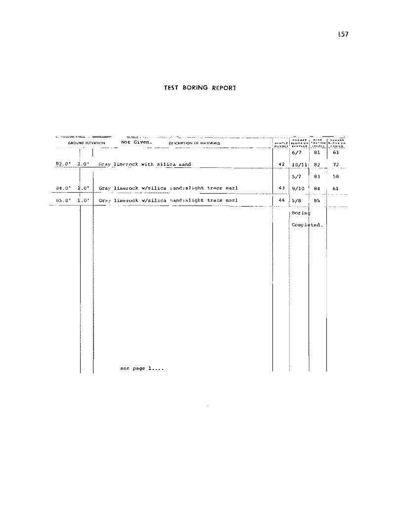
iS7

TEST BORING REPORT

"ROUN!) HfVA1'ON Not Given. O[SCRIf'ilON OF MATERIAlS

61

82 lime.ocK with silica sand -.... ------- - -- -._- ---------------1---- 72

S8

limerock w/silica c.and;slight trace lnarl 61

1imerock w/silica sand;slight trace marl

see page 1 ••••

158

TEST BORING REPORT

GROUNO fUVATIOH Not Given. OESClUPTION Of MAl ElIIAL$

3.5 ' 3. , 'ran medium fille silica sand with 1imereck 4.0' 0 • .9:. Dark gray medium fille si~ica sand

6.0' 12_0 'ran medium fine silica sand

9.0' 3.0 Brown medium fine silica sand w/slight trace roots

14.0' 5.0' Tan limereck wi 1:.'1 silica sand. trace mar.!

15.0' 1.0' 'ran limerock with silica sand; trace marl

ao.o· 5.0' Tan limerock with silica sand:irace marl ,

later letel : ~ _·bel.ow surface @ -r-- oate: See Above. 3-'Opm

I I MOMW" I ~C .... I~ .... w~1I. a ... O-_ ON ,. ..... TIO ..

~~,~

2/2 l. 2

6/6 ,2 1

10/10 3 1 !

1 ! 'fl/O , .. 2

9/10 5 21

3 13/15 6 2:

6/5 7 1

I 5/5 8 1

4 I 4/4 9 1.

4/5 10 l'

3/4 1l. 1;

-5/6 12 2'

13 2· -

5 14 2:

6 15 3:

5/6- 16 21

11/12 17 2:

18 2:

l.9 3,

7 20 3:

159

TEST BORING REPORT

I I ............. 1 ,. .. ,. .... .OM

GaOUHD WVATION DfSCIUPTIOH Of MATERIALS ....... ~& .... 0 ..... 0 ... TIll ... TIO ... .... 0 ...

See Pg. 1. ~~~ ...E.:!.!.

4/4 21 13

7/8 22 18

23 24

24 20

2~cO' 5 0' Tan lime rock ""i th silica sand' trace marl 8 25 22

2/3 26 16

6/6 Z7 n

28 3l. I ! 29 36

lO.....D' C;Q' Brown fine medium. silica sand ""ith slight trace limerock 9 30 38

2/3 31 14

5/6 32 2l.

33 32

34 41-

15.0 ' ~.Ol Tan fine medium silica sand 10 35 S4

2/3 36 19

6/6 37 28

38 34

39 38

·0.0' ~.O· Gray medium fine silica sand 11. 40 46

Water level: See Pg. ~.

160

TEST BORING REPORT

I ; W ...... IIIIIIC. I ... .:,..... I N"IIIIII'

CaOUNO !UVAT10N See Pg.. 1. OESOUYT.ON OF M.lA.TfRLAU :, .. ,. .. ~,-« 1_\.0""". OM ".ATtO,. 1.1..0 _ _____ , _--: ______________________________ I~ .~;~u ":o~. I cu;

7/8

'.5./'1 • Gray med~um fine silica sand 12 I

• S.O

SIS

6/6

;0.0' S.O· Gray medium fine silica sand wit-lot t:::.'ace 1imerock 13 i

4/5

7/7

5.0'

Gray medium fine silica sand with trace she11:s1ight

S .0 ", traCe marl 14 55

I 6/7 56

1.2/1:1 57 E

58

S9

(* " 5.0' Tan medium fine silica sand with trace li.merocx,mairl.shel,. 15 60

Water level: see page 1 •••

161

TEST BORING REPORT

....... IIl. ;.;;.;~:. G20UNO flfVATlON Not Given

oeSCliIPtlON 0' MA UI!IALS " .... """", _"'a ... o~ .,,:~~~: c .... J ~v .... ,.Y~".

7/8 61 4C

12/13 62 45

63 61

64 91

.0' 5.0 Gray fine si1~casand with some 1imerock 16 65 12

U/12 66 60

15/16 67 84

68 1C

69 92

.0' 5.0 Gray fine silica sand with some 1imerock 17 70 9C

lS/2C 72

26/24 1.3

7 10

L8/18 74

.0" 5.0 Grav fine silica sand with 1imerock 18 LO/14 75

see page 1. •• _

162

TEST BORING REPORT

G20UNO eUVAT10N No't. Given. DfSCltlPnON OF MArtRIAl.S I H ..... U I ,. .... I H ....

___ ~;__-... ------------------------.------' !::~!, •. :ct.::~:."1 TI~~~:~ .~~;J:

i

4.0' 4.0 'i Tan medium fine silica. sand 'With some l.i:neroek

S.O·

10.0' 5.0' Tan med.ium fine silica sand

o· 5.0

ate: leve.l.: 4.1

Tan medium fine silica. sand; trace shell. limerock

'below surface @ 3 : 05 pmoate: See AbOve.

1

3

4

5

2/2

6/6

19/10

110/12

14/5

8/9

8/8

ll/H

7/7

!S/5

3/2

2/3

1/1

1/2

1 1

2 3

3 10

4 14

!

7 10

8 14

9 15

10 11

II 10

12 10

13 9

14 9

15 10

16 5

17 6

18 5

19 6

20 8

163

TEST BORING REPORT

(HIQUND ruVATION See Pg:. 1. DESOJPTlON OF MAHRIALS :~::~~; •• ':..o::'~~."l "I~~T~~~ _",0 __ C

~

2/2 21 9

4/4 22 I

10

23 17

24 :H

zS.O' 5.0' Brown medium fine silica sand 6 25 26

2/3 26 12

5/6 27 16

28 21

29 26

10.0' p.o' Brown fine medium silica sand 7 30 34

3/4 31 IS

8/9 32 24

33 36

I 34 39

5.0' .0' Brown fine medium silica sand 8 51 35

I .3/3 I i 36 II

5/6 I 37 31

38 38

39 42

0.0' 5.0 Tan fine medium silica sand 9 51 40

Water 1evy1: See Pg. t.

164

TEST BORING REPORT

<>«OUND ruvATtON See Pg". 1. DESClIIPTtON 01 ..... 1 !~tAU 'A""~ •• ~~::~!-! '::!~I~~ .:~:*;c: ; "Y".C:" ...... '"-E:JII '''<lOT) ~

4/4 41 2(

6/6 42 2€

43 3J

44 3;

45.0' 15.0' Gray medium fine silica sand 10 4S 3:

5/6 46 2C

9/9 47 21

0 48 2~

49 3:

50.0' ~.Ol Gray mediwn fine silica. sand 11 50 5J

4/5 51 4}

9/10 52 51

53 7C

54 7E

i5.0· 5.0' Gray fine mediwn silica sand; t:race shell 1.2 55 91

6/6 56

I 54

12/12 57 6€

58 BC

Tan fine medium silica sand with t:rac:e limerock; 59 ~.:

slight t.:::ace =1 1.3 ,0 I)' 5.0 60 11

Water level: see page L •••

165

TEST BORING REPORT

Gl!OUNO WVATION Of5ClUPTION OF MAnRlll1..S :~::';! 1·~E·l:: TS~~~~ "AM

Not Given !.~~:,:

7/7 61 45

13/14 62 60

63 64

64 84 t

5.0' S.O 'j Gray fine silica sand wi~, some lime rock 14 65 10

11/13 66 60

10/10 67 71

68 10

69 90

LO I 5.0 Gray fine silica san~ with trace 1imerock , 15 70 11

16/18 71 90

21/24 n 98

i I

73 86

.l2/14 74

LO' I 5. a I Tan limerock and sand 16 18/18 7S

see paqe 1 •••

APPENDIX B

PREPARATION AND INSTALLATION OF MUSTRAN CELLS

169

PREPARATION AND INSTALLATION OF MUSTRAN CELLS

Due to the proven performance of the Mustran cell in axial load tests

of drilled shafts, their use is becoming quite prominent throughout the

United States. Because of the increased use of Mustran cells, the following

sections have been included in Appendix B.

Material List for Mustran Cell

Construction Sequence for Mustran Cell

Installation Procedure for Mustran Cell

170

MATERIAL LIST FOR HUSTRAN CELL

Following is a list of the materials needed for the construction of

a single Mustran cell.*

Item No.

1

2

3

4

5

C

7

8

9

10

11

12

l3

14

15

16

17

18

19

20

21

Quantity

1 each

1 each

1 each

2 each

1 each

2 each

as needed

as needed

as needed

as needed

as needed

as needed

as needed

as needed

as needed

as needed

2 each

1 each

as needed

4 each

as needed

MATERIALS

Description

top cap, steel (Fig. B.l)

bottom cap, steel (Fig. B.2)

centerpiece, steel (Fig. B.3)

mounting angles, steel (Fig.B.4)

gauge application tool set, ATS-2 (to be ordered only once)

strain gauge, EA-06-2S0TG-350

sandpaper, wet or dry silicon-carbide, 220 (SCP-l) and 320 (SCP-2) grit

cotton swabs, CSP-l

gauze sponges, GSP-l

M-bond 600 adhesive kit

M-coat D kit

M-coat G kit

chlorothene NU degreaser, CNU-l

M-prep conditioner A, MCA-2

M-prep neutralizer 5, MNS-2

Mylar JG tape, MJG-2

pressure pads and backup plates, GT-14 (reusable)

hargrave spring clamp, 1", HSC-l (reusable)

stranded-tinned copper wirp, red, black, green, and white, l26-BWV

bondable terminals, CTF-SOC (solder tabs)

TFE teflon film, TFE-l (reusable)

* Items 5-21 are all available from Micromeasurements; Micro-

measurement name and part number are given.

Drill and Tap for 1/8"4- Pipe Fitting

1/4" 4-

Top View

1-3/8"

I f il' I 1 I

I I I I I I fI) ! I I I I ~ ( I L_~

I- ~ = -,('----- I j'1 I

~ - I I r\, o 0. N I I I I - CD I I I II 0.0 .........

~ -Drill and Tap for--l....,

Drill and Tap to Fit 5/16"- 24 Thread on Centerpiece

Drill With -# 26 Bit Size

Countersink

~ rr>

Drill and Tap to Fit 5/16"-24 Thread on Centerpiece

(.0 = .........

(.0

I'- ......... I en

I

-~

171

'--+-- Drill and Tap for 6-32 Screw ~ 1/211 Deep

1/811 Pipe Fitting to J<--___ 2_1_1 ___ -..r

a Depth of 3/4 11

Side View

Fig. B.l Top Cap

172

Countersi nk

~r:

Top View

1- 3/8"

II/IS" II/tS"

I

-~ I I I I I<')

't' L .....

r' I I I I

2"

Side View

Drill and Tap to Fit 5/IS"-24 Thread on Centerpiece. Remove Threclds to Depth of 1/8"

Dri II and Tap to Fi t 5/IS"-24 Thread on Centerpiece. Remove Threads to Depth of 1/8 11

U) 10 ........ I"- ........

I (1) I

-00 ........

Drill and Tap for S-32 II D Screw AS 1/2 eep

Fig B.2 Bottom Cap

Top View

L. 490 " +.00111

l~t -.00" -, II

+ .490" + .001 - --J.- - .00

Note: I. Surface Grind a II Surfaces

5/16"- 2 Thread

2. All Surfaces Must Be Rust and Pit Free

Side View

4 ~ ~ 1= == t= ~ ~ i==

I

I

I

I

t=: t= ~ ~

--

-C\I ....... 1

= ( r

to -....... --::J 0 ~

CI) "C c::

::>

-0 q +1 = 0 lC)

lC)

= to -....... --::J 0 ~

CI) "C c:: =(1

r = C\I .......

5/1611-24 Thread- ~ t=: 1= --~ -

Fig. B.3 Centerpiece

C\I ....... -I to

173

174

T~=co I - -E~- - - - - - --

co ........ rt)

I rt)

........ I'-

= V ........

I C\J

- ~~ ------

~ I Round off ~~- I Corner

1/4" 1/4" 1" ~ 0/'

~ Front View

--\ Drill With # 26

/ Bit Size (.147")

1-1/411

Side View

Make With I/alix 1/2" Steel Strip and Bent to I~bove Dimensions

Fig. B.4 rlountine: Angles

Item No.

22

23

24

25

26

27

28

29

30

31

32

33

34

35

36

37

38

Quantity

as needed

as needed

as needed

as needed

1 each

2 each

as needed

1 each

1 each

1 each

1 each

as needed

4 each

2 each

1 each

1 each

1 each

Description

solder, low temperature

Belden wire, #8729, 22 AWG, stranded, 4-conductor,be1dfoi1 shei1ded plastic jacketed instrumentation cable, 0.265-inch O.D.

vacuum grease

teflon tape, 1/2-inch wide

radiator hose (Gates No. 1522H (24022)), 1 3lB-inch I.D., 8-inch length

hose clamps, radiator (ideal combo hex #5424 maximum clamp diameter - 2 inches)

silicone rubber sealant

male connector, Swage10k #B-400-1-2

front ferrule, Swage10k #B-403-1

back ferrule, Swage10k #B-404-1

tygon tubing, 1/4-inch I.D., 3lB-inch O.D. , 1-inch length

Scotch cloth tape, #390, olive drab, 3-inch, or 3-inch silver duct tape

bolts, 6-32 with 1/2-inch thread

nuts, 6-32

male connec tor, Swage 10k ffB-600-1-4 (to be ordered only once)

back ferrule, Swage10k #B-604-1

front ferrule, Swage10k #B-603-1

CONSTRUCTION SEQUENCE FOR MUSTRAl;r CELL

Following is a step-by-step process for constructing a Mustran cell.

1. Inspect centerpiece; make sure it meets specifications. Check

end caps by screwing onto centerpiece.

2. Choose the two best opposite sides of the centerpiece for strain

gauge application.

3. Remove grease from centerpiece.

175

176

4. Mark centerpiece, vertical and horizontal scribe marks, for

centering of strain gauge (both sides), Scribe marks should not go into

gage area.

5. Apply M-prep conditioner and sand the centerpiece gauging area

with 220 or 320 silicone (both sides).

6. Neutralize complete bar with M-prep neutralizer.

7. Clean area to be gauged with Ch10rothene Nu degreaser ,. using a

cotton swab to wipe area. (Fig. B.S shows centerpiece after steps 1-7.)

8. Lay strain gauge and 4-termina1 solder tab (solder tab will be on

only one side of centerpiece) on glass plate and clean with Ch1orothene

Nu degreaser. Use cotton swabs.

9. Place strain gauge (and solder tab if needed) on l'1y1ar tape so

tha t the gauge s ide is agains t the tape. This is done by laying the gauge

and tab (tab should be at vertical end of strain ~uge) on the glass plate,

~ge side up and putting the Mylar tape on the strain gauge and tab.

10. Position the gauge/tape assembly so the alignment marks on the

gau~ are in line with the alignment marks on the centerpiece. Holding

the tape at a shallow angle (about 45°), place the assembly onto the center

piece surface. If the ~uge appears to be misaligned, lift one end of the

tape at a shallow angle until the assembly is free, then realign. (See

Fig. B. 6. )

11. Once alignment is correct, lift the unanchored end of the tape

at a shallow angle until gauge and terminal are free of specime.n surface.

12. Tuck the loose end of tape under and press to the surface of the

centerpiece so the gauge lies flat with the bonding side exposed. (See

Fig. B. 7. )

n'

flO . 1.1 S"Un "' . ,. and C.ncor~ Lo<. Ilead)o to, ~p"U< .. I •• of .... """" ~

179

13. Apply thin coat of M-bond 600 to back of gauge and to centerpiece

gauge area. Allow this to air dry for 5 to 20 minutes. (See Figs. B. 8 and B.9.)

14. Set strain g:luge in place; lift tucked-over end of tape and stra:in

o gauge over the gauge area of centelpiece at approximately a 30 -angle. ';hth

a piece of teflon, slowly make a single wiping stroke over the gauge/tape

assembly, bringing the gauge down over the alignment marks on the center-

piece. (See Fig. B .10. )

15. Place teflon guard (TFE teflon film) over the strain gauge and

Mylar tape; tape teflon guard to centerpiece. (See Fig. B.ll.)

16. Repeat steps 7-15 for opposite side strain gauge placement. Be

sure that the horizontal and vertical grids on the strain gauges match on

both sides.

17. Place pressure pads and backup plates over the strain gauges

(teflon guards still in place).

18. Clamp the pressure pads and backup plates with the Hargrave

spring clamp. (See Fig. B.12.)

19. Place entire assembly in preheated oven for temperature curing

(250°F for 2 hours).

20. After temperature curing, allow centerpiece to cool gradually to

room temperature.

21. Remove clamps, pressure pads and backup plates, and teflon guard.

22. Carefully peel off the Mylar tape. (Fig.B.13a and b show strain

gauges on both sides of centerpiece after step 22.)

23. Check for stram-gauge bonding and for air bubbles underneath

strain gauge.

24. Apply solder dots to gauge tabs and to 4-terminal solder tab.

Solder wiring between the gauges (Fig. B.14). (Fig. B.15 shows centerpiece

after step 24.)

181

Fig . B. 10 Laying of St rain Gauge

182

Fig. B.Il Placement of Teflon Pads

Fig. B. 12 Clamp and Pressure Pads

Fig . B.13 (a) (b )

Strain Gauge on Back of Centerpiece Strain Ga uge and Tab on Front of Centerpiece

183

(.)

(b)

184

Leads From Beldon Cable

Front

p+ Green~ S+ White ____ --t--J

p- Black _-f-------J

S- Red ~

Fig. B.14. Wiring Between Gauges

I~ear

185

25. Attach strain indicator and check gauge for balance and operation.

26. Cut Belden cable #8729 to required length and label it by using

the 3-inch-wide tape and also by writing on the cable; a waterproof marker

should be used.

27. Remove approximately 6 in of outer sheath at one end of the

Belden cable.

28. Put the top of a Swagelok #B-400-l-2 male connector on the end

of the cable where the outer sheath was removed.

29. Put back ferrule, Swagelok #B-404-1, on same end of cable.

30. Put front ferrule, Swagelok #B-403-1, on same end of cable.

31. Put teflon tape on threads of the bottom of a Swagelok #B-400-l-2

male connector.

32. Attach the bottom of the male connector to the top cap.

33. Insert the lead wires from the Belden cable through the Swagelok

male connector and top cap. At this time on~ should be able to screw the

top and bottom of the Swagelok male connector back together, with the front

and back ferrules in place.

34. Securely attach top cap to centerpiece so that the top cap is on

the end closest to the 4-terminal solder tab.

35. Strip approximately 1/4 in of each lead wire from the Belden

cable.

36. Solder the four lead wires from the Belden cable to the solder

tabs.

37. Check the wiring with portable strain indicator for balance and

with OHM-meter for resistance to ground.

'K

"I. I . U WIrL .... _. C ..... , P'o.' ."" I.ok o[ c. ••••• , •••

38. Apply one coat over all wiring connections with M-coat D. Allow

30 minutes for drying (Fig. B.16).

39. Coat all gauges and exposed wiring with heavy application of

M-coat G (Fig. B.17). Allow 24 hours for drying. Caution: do not coat or

plug cable entrance hole through top cap.

40. Cut proper length (8 in) of radiator hose.

41. Put two hose clamps loosely on the radiator hose.

42. Apply silicone rubber sealant to both the top and bottom caps.

43. Insert the centerpiece and top cap (up to the 2-inch-diameter

lip) in the radiator hose, at the same time trapping the ground wire

between the top cap and radiator hose.

44. Securely attach bottom cap to centerpiece. After this point, if

for any reason the Mustran cell needs to be taken apart, the radiator hose

should be cut off. This is to prevent the wires from being torn loose.

45. Center the radiator hose and clamp.

46. Cut off the ground wire that is sticking out of the radiator

hose.

47. Drill hole (#26 bit size) in lip of bottom cap to coincide with

hole in lip of top cap.

4S. Secure attaching brackets to top and bottom caps, using

187

4-6-32 X 1/2 bolts and 2-6-32 nuts. (Fig. B.lS shows assembled Mustran cell.)

49. Remove approximately 6 inches of outer sheath from the other

end of the Belden cable.

50. Strip approximately 1/2 inch of each of the four lead wires.

51. Insert the lead wires and approximately 3 inches of the Belden

cable through the 1/4-inch tygon tubing.

,.

'"'I. 1 . 11 "" .. _bl.4 _.r .. toll

52. Put the top of a Swage 10k #B-600-l-4 male connector on the tygon

tubing (bottom of male connector is in manifold).

53. Put the back ferrule, Swagelok #B-604-l, on the tygon tubing.

54. Put the front ferrule, Swagelok #B-603-l, on the tygon tubing.

PROCEDURE FOR MUSTRAN CELL IHSTALLATTON

The following is a set of instructions for installing Mustran cells

on a reinforcing steel cage.

1. After unpacking the cells, check them with a portable strain indi

cator to see if they will balance and with an Ohm-meter for resistance to

ground, which should be infinite.

2. Measure the length of the reinforcing cage.

3. Mark off the placement depths of the Mustran cells.

4. Starting at the bottom of the reinforcing cage, mount the Mustran

cells at the placement depths that were marked off. (The bottom level and

the top level should both contain at least four Mustran cells.)

5. Cells should be mounted so that the end with the Swagelok fitting,

the top cap. will be pOinting to the bottom of the drilled shaft.

6. Mounting should be done so that any level of 2 or 4 that the cells

should be approximately 180 0 or 90 0 apart. (See Fig. B.19.)

189

9. String the cable out on the interior of the reinforcing cage and

out the top of the reinforcing cage. After four levels of cells have been

installed, two cells on each of the four rebars being used, the cable should

be taped to the rebars for the complete length of the shaft.

190

Fig. B.19 Mounting of Mustran cells

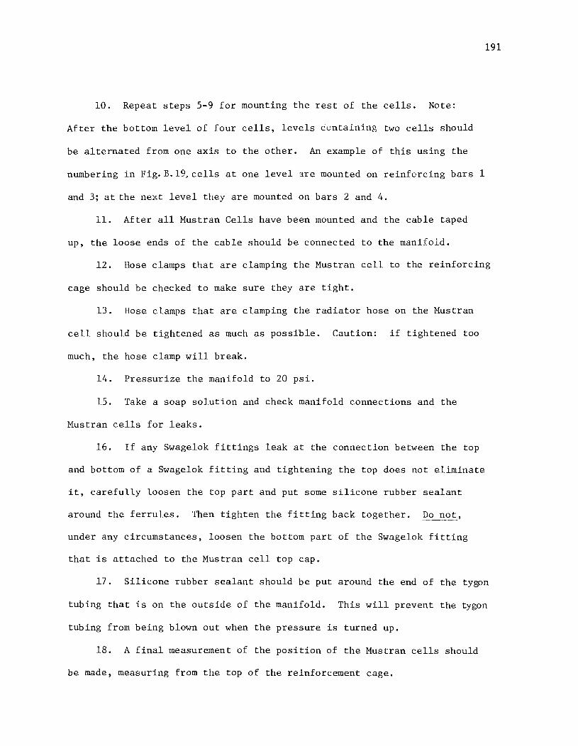
10. Repeat steps 5-9 for mounting the rest of the cells. Note:

After the bottom level of four cells, levels containing two cells should

be alternated from one axis to the other. An example of this using the

numbering in Fig.B.19, cells at one level ~re mounted on reinforcing bars 1

and 3; at the next level they are mounted on bars 2 and 4.

11. After all Mustran Cells have been lnounted and the cable taped

up, the loose ends of the cable should be connected to the manifold.

191

12. Hose clamps that are clamping the Mustran cell to the reinforcing

cage should be checked to make sure they are tight.

13. Hose clamps that are clamping the radiator hose on the Mustran

cell should be tightened as much as possible. Caution: if tightened too

much, the hose clamp will break.

14. Pressurize the manifold to 20 psi.

15. Take a soap solution and check manifold connections and the

Mustran cells for leaks.

16. If any Swagelok fittings leak at the connection between the top

and bottom of a Swagelok fitting and tightening the top does not eliminate

it, carefully loosen the top part and put some silicone rubber sealant

around the ferrules. Then tighten the fitting back together. Do not,

under any circumstances, loosen the bottom part of the Swagelok fitting

that is attached to the Mustran cell top cap.

17. Silicone rubber sealant should be put around the end of the tygon

tubing that is on the outside of the manifold. This will prevent the tygon

tubing from being blown out when the pressure is turned up.

18. A final measurement of the position of the Mustran cells should

be made, measuring from the top of the reinforcement cage.

192

19. Before the reinforcement cage is placed in the exc~vation, the

pressure should be turned up to the "final" pressure and checked for leaks.

C'Final" pressure is approximately equal to depth of excavation. Example:

excavation is 60 ft; "final" pressure equals 60 psi. "Final" pressure

should never be lower than 20 psi.)

20. The manifold should be attached to the reinforcement cage

approximately 15 feet from the top of the cage so that the cables are

hanging fairly straight. The pressure should be at the "final" pressure.

21. As the reinforcing cage is being lowered into the excavation,

the lowering of the cage should stop when the manifold is in a position

that it can be removed from the cage.

22. Once the manifold is removed, the cage is lowered che rest of

the way into the excavation. The manifold should be walked out away from

the excavation as the cage is lowered.

23. This step is applicable only if there is a casing to be removed.

The cables and the manifold should be put inside the reinforeement cage

and the manifold attached to the cage when the concrete is w:~thin approxi

mately two feet of the surface or when the contractor decides to pull the

casing. After the casing is pulled, the manifold should be removed and

cleaned.

24. After the concreting has been completed, a measurement from the

ground surface to the top of the reinforcement cage should be made.

25. The "final" pressure should be kept on the system for at least

four days. After this the pressure may be set at one-half the "final"

pressure, but not less than 20 psi, of the test.

APPENDIX C

TYPES OF INTERNAL INSTRUMENTATION FOR USE IN DRILLED SHAFTS FOR MEASUREMENT OF AXIAL LOADS AS A FUNCTION OF DEPTH

APPENDIX C. TYPES OF INTERNAL INSTRUMENTATION FOR USE

IN DRILLED SHAFTS FOR MEASUREMENT OF

AXIAL LOADS AS A FUNCTION OF DEPTH

The making of Mustran cells and their use are described in some detail in

this report for the purpose of making information available to any potential

uses. The cells are not patented and may be constructed and used by anyone.

However, there are other types of instrumentation that can be used successfully.

Several of these were discussed in detail by Barker and Reese (1969) and only

a brief presentation is made here.

Telltales. A telltale is a bar that is placed in a tube that is cast in

the shaft. When a load is applied, the tube will strain but the bar, if

installed properly, will not change in length. Thus, with the bar as a

reference, an ordinary dial gauge can be used to obtain the shortening in a

shaft from the top of the shaft to the bottom of the bar. If several telltales

are installed in a test shaft, the downward movement of various points along

the shaft can be obtained almost directly. Differentiation of the deformation

curve will yield the strain in the shaft. The internal load can then be

obtained if the axial stiffness of the shaft is known.

Weldable Strain Gauges. A strain gauge is manufactured by Micro

Measurements, P. O. Box 27777, Dept. TR, Raleigh, North Carolina 27611, that

can be fastened directly to a rebar by use of a special welding tool. The

gauges are made in the factory with a protective copper tube over the lead

wires from the gauge to the end of the wire. Thus, each gauge is waterproofed.

The gauge can be read with an ordinary strain indicator.

195

196

Bar Strain Gauge. A device is manufactured by Jido Seigyo Giken Co.,

Ltd., 5-10-14, Kamiidedai, Ohta-ku, Tokyo 145, Japan, that em'?loys a linear

variable differential transformer in a strain gauge that will replace a

section of a rebar. The rebar is cut, the special gauge about 17.5 in. in

length is welded into place, and lead wires are brought to the top of the

drilled shaft.

Removable Extensometer. The Laboratoire Central des Ponts et Chaussees,

Paris, ha& developed a special extensometer that can be placed in a drilled

shaft and removed after the load test is completed. One or more pipes,

approximately 2 in. in inside diameter, are cast from top to bottom of the

shaft. After the concrete has set and before the test is started, the

extensometer is lowered into the pipe. The extensometer consists of a series

of "blockers" that are connected by thin metal tapes on which strain gauges

are attached. The blockers can be activated with compressed a.ir so that they

expand and engage the inside of the pipe. The lower blocker is expanded, the

system is loaded at the ground surface so that the metal tapes are prAstressed

to an acceptable degree, and then the other blockers are expanded. As a load

is applied to the top of the shaft, the prestress in the tape is reduced and

the strain from point to point along the shaft is obtained.

Other Devices. A number of other devices or systems can be employed.

Two of these devices are used in Europe and have not been marketed in the U.S.

to any extent; they are the vibrating wire strain gauge and the Gloetzl cell.

Each of these devices can be embedded in concrete and used to obtain the

distribution of load.

Some investigators have used load cells to extend across the entire cross

section of the shaft. The cells are expensive, time-consuming to install, and

197

construction difficulties can result. Also, a rebar cage cannot be employed

with such load cells.

APPENDIX D

CONSTRUCTION SITUATIONS WHERE CASING WOULD BE DIFFICULT TO REMOVE

APPENDIX D. CONSTRUCTION SITUATIONS WHERE CASING

WOULD BE DIFFICULT TO REMOVE

There are a large number of circumstances in the construction of drilled

shafts that would lead to the sticking of a casing (personal communication

from Mr. Glyen Farmer). Short descriptions of some of these instances are

given in the following paragraphs.

The most common situation is where the casing has to be seated into a

strong formation. Some bedrock where casing would be used will have a htgh

compressive strength, perhaps more than 1000 psi. The bond on the outside of

the casing can in turn be high, leading to a large tensile force that would be

needed to withdraw the casing. The contractor should make some trials during

the initial phases of construction so that the casing is seated no more than

necessary.

Another undesirable situation occurs when a hole is drilled through sand

or other cohesionless soil and when an obstruction is encountered in the

drilling that causes the auger to be displaced. Thus, the drilled hole will

not be plumb and straight. When the casing is installed it will bear against

the side of the excavation. The pulling resistance will, of course, be

increased over that of normal construction.

As noted in Chapter 1, in most instances the excavation is usually made

with drilling fluid prior to placing a casing. After the placing and seating

of the casing, the slurry is removed from inside the casing so that the

excavation can be advanced in the dry to the design depth. If a seal has not

been made properly, the drilling fluid in the annual space behind the casing

201

202

will flow into the excavation, allowing the soil behind the casing to collapse.

Thus, the pulling resistance will be increased.

The last problem to be mentioned relates to improperly dE!signed concrete.

If there is a pour requiring a large volume of concrete, if the haul from the

mix plant is long, if the weather and concrete materials are hot, the concrete

can partially harden during the pouring operation. In such a case the pulling

resistance will be increased by the extra frictional resistance of the concrete

inside the casing. This problem can be solved by the proper design of a

concrete mix and by good inspection procedures.

Leaving casing in place can be avoided in many cases if the contractor

has a service crane of sufficient capacity on the job. Some contractors have

available service cranes of only 40-ton capacity and others have cranes of

100-ton capacity or larger. Obviously, the larger crane is more effective in

pulling the casing.

However, if there is great difficulty at a given site in removing the

casing even when good construction procedures are employed, consideration

should be given to the use of the slurry displacement method of construction.

REFERENCES

1. American Petroleum Institute, API Recommended Practice for Planning, Designing, and Constructing Fixed Offshore Platforms, American Petroleum Institute, January 1980.

2. Arias, Robert P., "Evaluation of Drilled Shaft Integrity by NonDestructive Methods," Master's thesis, University of Texas at Austin, Civil Engineering, December 1977.

3. Barker, W. R., and L. C. Reese, "Instrumentation for Measurement of Axial Load in Drilled Shafts," Research Report 89-6, Center for Highway Research, The University of Austin, November 1969.

4. Barker, W. R., and L. C. Reese, "Load-Carrying Characteristics of Drilled Shafts Constructed with the Aid of Drilling Fluids," Research Report 89-9, Center for Highway Research, The University of Texas at Aust~n, August 1970.

5. Coyle, Harry M., and Reno R. Castello, "New Design Correlations for Piles in Sand," Journal of the Geotechnical Engineering Division, ASCE, Vol. 107, No. GT7, July 1981.

6. Engeling, Don, and L. C. Reese, "Behavior of Three Instrumented Drilled Shafts under Short-Term Axial Loading," Research Report 176-3, Center for Highway Research, The University of Texas at Austin, 1974.

7. Fuller, F. M., and H. E. Hoy, "Pile Load Tests Including Quick-Load Tests Methods, Conventional Methods, and Interpretation," Highway Research Record Number 333, Pile Foundations, Washington, D.C., 1970, pp. 74-86.

8. Meyerhof, G. G., "Bearing Capacity and Settlement of Pile Foundations," Journal of the Geotechnical Engineering Division, ASCE, Vol. 102, No. GT3, March 1976.

9. Oneill, Michael W., and L. C. Reese, "Load Transfer in a Slender Drilled Pier in Sand," ASCE Spring Convention and Exhibit, Preprint 3141, Pittsburg, PA., 1978.

10. Quiros, Gerardo W., and L. C. Reese, "Design Procedures for Axially Loaded Drilled Shafts," Research Report 176-5F, Center for Highway Research, The University of Texas at Austin, 1977.

203

2M

11. Peck, Ralph B., W. E. Hanson, and T. H. Thornburn, Foundation Engineering, second edition, John Wiley & Sons, New York, 1973.

12. Reese, Lymon C., and S. G. Wright, "Construction Procedures and Design for Axial Loading," Drilled Shaft Manual, Vol. l., U. S. Department of Transportation, Offices of Research and Development, Washington, D.C., July 1977.

13. Touma, Fadlo, and L. C. Reese, "The Behavior of Axially Loaded Drilled Shafts in Sand," Research Report 176-1, Center for Highway Research, The University of Texas at Austin, 1972.

The Influence of a Steel Casing on the Axial Capacity of a ... · axial capacity of drilled shafts...

Documents

Transcript of The Influence of a Steel Casing on the Axial Capacity of a ... · axial capacity of drilled shafts...