The increasing happiness of US parents - Chris M....

The increasing happiness of US parents

Chris M. Herbst1 • John Ifcher2

Received: 5 December 2014 / Accepted: 10 July 2015 / Published online: 19 July 2015

� Springer Science+Business Media New York 2015

Abstract Previous research suggests that parents may be less happy than non-

parents. We critically assess the literature and examine parents’ and non-parents’

happiness-trends using the General Social Survey (N = 42,298) and DDB Lifestyle

Survey (N = 75,237). We find that parents are becoming happier over time relative

to non-parents, that non-parents’ happiness is declining absolutely, and that esti-

mates of the parental happiness gap are sensitive to the time-period analyzed. These

results are consistent across two datasets, most subgroups, and various specifica-

tions. Finally, we present evidence that suggests children appear to protect parents

against social and economic forces that may be reducing happiness among non-

parents.

Keywords Parents � Happiness � Life satisfaction � Subjective well-being �General Social Survey (GSS) � DDB Lifestyle Survey (LSS)

JEL Classification D60 � D10

& Chris M. Herbst

[email protected]

John Ifcher

[email protected]

1 School of Public Affairs, Arizona State University and IZA, 411 N. Central Ave., Ste. 450,

Phoenix, AZ 85004-0687, USA

2 Department of Economics, Santa Clara University, 500 El Camino Real, Santa Clara,

CA 95053, USA

123

Rev Econ Household (2016) 14:529–551

DOI 10.1007/s11150-015-9302-0

http://crossmark.crossref.org/dialog/?doi=10.1007/s11150-015-9302-0&domain=pdf

http://crossmark.crossref.org/dialog/?doi=10.1007/s11150-015-9302-0&domain=pdf

1 Introduction

A large body of research generally finds that parents are less happy, experience

more depression and anxiety, and have less fulfilling marriages than their childless

counterparts (e.g., Alesina et al. 2004; Clark 2006; Clark et al. 2008a; Di Tella et al.

2003; Evenson and Simon 2005; Glenn and McLanahan 1982; Nomaguchi and

Milkie 2003; Stanca 2012; Grossbard and Mukhopadhyay 2013).1 Such findings are

perhaps unsurprising given that parents report enjoying childcare only slightly more

than housework and commuting (Kahneman et al. 2004). The existence of a

parental happiness deficit has been adopted by some as conventional wisdom and

become the focus of numerous pieces in high-profile media outlets, for example,

‘‘Does Having Children Make You Unhappy?’’ by Lisa Belkin (New York Times,

April 1, 2009), ‘‘Kid Crazy: Why We Exaggerate the Joys of Parenthood’’ by John

Cloud (Time, March, 2011), and ‘‘Having Kids Makes You Unhappy, Right?’’ by

Betsey Stevenson (National Public Radio’s Marketplace, May 6, 2010).

Yet despite—or perhaps because of—the acceptance of this finding, we know of

only one attempt to critically assess the literature. Therefore, our first goal is to

undertake such an investigation. We uncover a number of potentially serious

problems. First, previous studies that use repeated cross-sections of happiness data

specify an empirical model that yields an estimate of the average parental happiness

gap over several decades. Implicit in this framework is that the happiness gap

remains constant over time. If, however, parents’ happiness followed a different

trend than non-parents’ happiness, this assumption would be violated and the

parental happiness gap may be mischaracterized. Second, previous studies generally

define a parent as anyone who reports having a positive number of children in

response to a question similar to the following: ‘‘How many children have you ever

had? Please count all that were born alive at any time (including any you had from a

previous marriage)?’’ This definition commingles noncustodial parents and empty

nesters with parents who are actively parenting, and commingles adoptive and step

parents with non-parents.

In light of these concerns, the primary goal of this paper is to examine whether

the evolution in US parents’ happiness differed from that of non-parents over the

past few decades. To our knowledge, this is the first paper to explore trends in

parental happiness. Further, our paper is focused on a well-defined set of parents,

those who are actively parenting. Our analysis uses data from the General Social

Survey (GSS) and DDB Worldwide Communications Life Style Survey (LSS), two

nationally representative datasets that have tracked self-reported happiness and life

satisfaction, respectively, over the last few decades. We find evidence that suggests

that parents’ happiness increases over time relative to non-parents. This relative

improvement appears to be the result of an absolute decline in non-parents’

happiness over time. Our findings are consistent across two nationally representative

surveys and virtually every demographic sub-group.

1 A few studies find inconsistent or neutral effects (e.g., Cleary and Mechanic 1983; Gore and Mangione

1983), and a few others find positive effects (e.g., Ross and Huber 1985; Aassve et al. 2009).

530 C. M. Herbst, J. Ifcher

123

Our results are interesting in light of recent studies documenting widespread

declines in happiness over the past few decades in the US For example, Herbst

(2011) finds that both men and women’s happiness declined between 1985 and

2005; and Stevenson and Wolfers (2009) find that women’s happiness declined

absolutely, and relative to men’s, between 1972 and 2008. In contrast, we find that

parents do not experience an absolute drop in happiness and are becoming happier

relative to their childless peers. This finding builds on previous research that

focused exclusively on low-income single mothers, and found that their absolute

and relative happiness (compared to low-income single childless women) increased

over the past few decades (Herbst 2012; Ifcher and Zarghamee 2014).

Lastly, we discuss three potential explanations for our findings. First, does being

a parent protect adults against a growing number of social and economic forces,

such as the reduction in social and political trust, the fraying of community ties, and

increasing narcissism, that may be reducing well-being in the US (Putnam 2000;

Twenge and Campbell 2009)? Second, is the observed relative increase in parental

happiness a reflection of a compositional shift in who is a parent? Third, it is

possible that perceptions regarding gender roles and the division of labor in the

household, as well as the utility of marriage and children, have evolved differently

over time for parents and non-parents?

2 Literature review

The earliest studies in the literature focus primarily on outcomes related to parental

depression, anxiety, and social relationships. Much of this work is thoroughly

reviewed in McLanahan and Adams (1987), Ross et al. (1990), and Umberson and

Williams (1999). In recent years, scholars interested in subjective well-being (SWB)

have begun to explore the relationship between parental status and happiness. The

happiness literature is summarized in Blanchflower (2008), Clark et al. (2008a, b),

and Dolan et al. (2008). In addition, Hansen (2011) provides a thorough review of

the parental happiness literature across multiple disciplines. Our intent here is to

highlight key findings and identify weaknesses in the literature.

The early literature provides fairly consistent evidence that parents are worse off

than non-parents across a variety of psychological domains (e.g., Barnett and

Baruch 1985; Evenson and Simon 2005; Glenn and McLanahan 1981, 1982; Glenn

and Weaver 1978, 1979; Nomaguchi and Milkie 2003; Pearlin 1974). Parents report

higher levels of stress and anxiety, increased anger and depression, and lower levels

of happiness and life satisfaction. Although the negative mental health associations

are concentrated among parents with children currently in the home, recent studies

find that well-being does not rebound substantially after children leave the home

(Evenson and Simon 2005). Furthermore, it appears that parents of young children

are unhappier still (Umberson and Williams 1999), and that each successive child in

the home is associated with steeper reductions in well-being (Glenn and McLanahan

1982). It must be noted, however, that a few studies find inconsistent or neutral

relationships (e.g., Cleary and Mechanic 1983; Gore and Mangione 1983), while

others find positive relationships (e.g., Ross and Huber 1985; Aassve et al. 2009).

The increasing happiness of US parents 531

123

Studies also indicate that parents are not a monolith. For example, female parents

worry more and experience lower levels of well-being than male parents (Bird and

Rogers 1998), and employed parents—especially working mothers—experience

lower mental health than unemployed childless adults (Simon 1998). The negative

relationship between parental status and mental health appears to be concentrated

among young parents, as a number of studies find that older parents have similar or

even higher levels of well-being than comparable non-parents (Koropeckyj-Cox and

Call 2007). Finally, single parents are substantially more likely to experience stress

and depression than their married counterparts (Aneshensel et al. 1981).

A smaller literature examines the association between parental status and marital

satisfaction and social connectedness. This research finds that marital satisfaction

decreases after the birth of the first child and does not return to pre-child levels after

the departure of the last child from the household (Lavee et al. 1996; MacDermid

et al. 1990; Menaghan 1982). In contrast, parents report higher levels of self-esteem

than non-parents (Hansen et al. 2009). Furthermore, a related set of papers

highlights the social benefits of parenthood through increased connectedness to

friends, family, and the community (Gallagher and Gerstel 2001; Umberson and

Gove 1989). Finally, a paper by Nomaguchi and Milkie (2003) finds that new

parents experience greater social integration (defined as the frequency of contact

with friends and relatives) than non-parents.

A number of recent papers have largely reached the same conclusion: parents are

less happy than non-parents. Most of this research focuses on global measures of

SWB and typically find that being a parent is associated with lower SWB (e.g.,

Alesina et al. 2004; Di Tella et al. 2001, 2003; Clark 2006; Clark et al. 2008a, b;

Stanca 2012). There is some disagreement in the literature, however, with some

studies finding neutral or positive effects (e.g., Frey and Stutzer 2006).2 Another

paper finds that, although children are not directly associated with parental

happiness, they do appear to negatively affect the spousal relationship—specifically,

by lowering spousal affection—which in turn reduces happiness (Grossbard and

Mukhopadhyay 2013). In addition, a paper by Helliwell and Wang (2011) finds

elevated levels of SWB during the weekend are more pronounced for those in their

prime parenting years presumably because the stress and time constraints associated

with being a parent are lessened during the weekend.

Our assessment of the literature uncovers the following: First, the standard

empirical specification in studies using repeated cross-sections yields an estimate of

the average parental happiness gap over time. For example, Di Tella et al. (2001,

2003) estimate the average association between parental status and happiness over

approximately 17 years of Eurobarometer data. Implicit in this framework is that

the parental happiness gap remains constant over time. If, however, parents and

non-parents follow different happiness time trends, then previous research

potentially mischaracterizes the parental happiness gap. The only exception is

McLanahan and Adams (1989), which compares the parental SWB gap in 1957 and

2 A recent paper by Hagstrom and Wu (2014 onlinefirst) asks a slightly different question: whether there

are happiness differences by pregnancy status. The paper finds that pregnancy results in a happiness

increase for white and Hispanic individuals, but not for black individuals (i.e., a neutral association).


123

1976 using two cross-sections of the Americans View Their Mental Health Survey.

Therefore, the current study fills this void by conducting an explicit trends analysis

of parents and non-parents’ SWB.

Second, there appears to be little consistency in the manner in which the

definition of parent is handled. For example, studies sometimes do not discuss

which groups of parents fall within their definition (e.g., full- vs. empty-nest

parents), nor is there much discussion of the advantages and disadvantages of the

chosen definition.3 Alesina et al. (2004) and Di Tella et al. (2001, 2003) do not

explicitly define their parent variable. Among papers that explicitly define the parent

variable, there is considerable variation in the definition. Margolis and Myrskyla’s

(2011) definition is based on the survey question ‘‘Have you had any children?’’

This is arguably narrow in scope in that it presumably omits adopted and step

children. It also does not allow one to distinguish between full- and empty-nest

parents. This distinction is potentially important in light of research that indicates

that the presence or absence of a child in the home can lead to different conclusions

about parental well-being (e.g., Evenson and Simon 2005).4 The survey used in

Kohler et al.’s (2005) analysis asks explicitly about respondents’ biological

children, thereby excluding adopted, step, and foster children. Lastly, Nomaguchi

and Milkie’s (2003) definition only includes new parents.

3 Data and methods

We examine parental SWB using two nationally representative repeated cross-

section surveys: the GSS and LSS. The GSS is a standard survey for studying US

SWB. The GSS was administered annually to approximately 1500 individuals

between 1972 and 1993 (with the exception of 1979, 1981, and 1992) and was

administered biennially to approximately 4500 individuals thereafter. For this study

we have obtained GSS data through 2008. The GSS includes a standard global

happiness question. Specifically, it asks respondents ‘‘Taken all together, how

would you say things are these days—would you say that you are very happy, pretty

happy, or not too happy?’’ This question has remained intact since 1972, providing

approximately 35 years of data and 42,000 observations.

There have been some changes to the GSS that might impact happiness trends.

Stevenson and Wolfers (hereafter SW) (2008, 2009, 2010) have written a series of

papers examining SWB trends using the GSS. We largely follow their methodology

for creating a consistent measure of happiness. This includes (1) dropping the Black

oversample in the 1982 and 1987 GSS; (2) dropping surveys that were conducted in

Spanish (and could not have been completed in English) in the 2006 GSS; and (3)

using the GSS weight WTSSALL to help ensure that the survey includes a

nationally representative sample of US adults [see Appendix A of SW (2008) for

3 A noteworthy exception is a recent paper by Myrskyla and Margolis (2014), which provides a detailed

discussion of the parent definition.4 However, it is the case that Margolis and Myrskyla (2011) retain only those parents with children under

age 18; thus very few empty-nesters are likely to be included in the sample.


123

additional details]. Our weighting strategy diverges from SW in one way.

Specifically, the question that directly preceded the happiness question was

different in the 1972 and 1985 GSS [Dillman et al. (1996) and Schuman and Presser

(1981) find a question-order effect]. We adjust for this by dropping all observations

from the 1972 and 1985 GSS as well as all observations from the split-ballot

experiments that were conducted in the 1980, 1986, and 1987 GSS to identify the

question-order effect. In contrast, SW create a weight to adjust for the question-

order effect using the split-ballot experiments. We chose our approach because we

believe it is more conservative. Given the large number of waves in the GSS,

dropping these observations should not impact the findings. Moreover, the results

are similar if we use SW’s weights.

Our second data source is the LSS [see Putnam and Yonish (1999) and

Groeneman (1994) for an extensive introduction to and evaluation of the LSS]. The

LSS is a proprietary data archive, although the 1975–1998 surveys are available on

Robert Putnam’s Bowling Alone website. Each year since 1975, the advertising

agency DDB Needham has commissioned Market Facts, a commercial polling firm,

to administer the LSS on a sample of approximately 3500 Americans. The

questionnaire covers a diverse set of topics, ranging from consumer behavior and

product preferences to recreational activities and political attitudes. Importantly for

the current study, the LSS contains a standard item that inquires about respondents’

life satisfaction: ‘‘I am very satisfied with the way things are going in my life these

days’’ (response categories include 6 = definitely agree, 5 = generally agree,

4 = moderately agree, 3 = moderately disagree, 2 = generally disagree, and

1 = definitely disagree). This question has remained intact since 1983. In auxiliary

analyses, we examine other SWB measures, for example, regrets about the past,

self-reported physical condition, and a variety of stress-related health issues.

Finally, between 1975 and 1984, the LSS was administered exclusively to married

individuals. Thus, we are only able to use the LSS data between 1985 and 2005,

providing approximately 20 years of data and 75,000 observations.5

3.1 Definition of parent

We define a parent as a respondent who reports having children ages 0–17 residing

in the household. This definition enables us to focus on the subset of parents who are

of primary interest—those who are actively parenting.6 We are not able to

determine whether the child is the respondent’s biological, adoptive, or step child,

or whether another household member claims legal guardianship over the child.

Although it would be ideal to examine parental well-being across each parent–child

5 The LSS includes a weight, but there is insufficient documentation on how the weight is constructed.

Therefore, we conduct the LSS analyses without the weight. Nevertheless, applying the weight does not

change the results.6 If women are more likely than men to gain custody of their children after separation or divorce, then

our definition of parent will result in a greater percentage of women being classified as parents than men

(35 and 41 % of men and women in our sample are coded as parents, respectively). As discussed in the

subgroup analysis in Sect. 4, the main results hold for men and women in both datasets [see Column (3)

of Table 6].


123

custody arrangement, it is somewhat reassuring that parents in most arrangements

are found to report similar SWB (Evenson and Simon 2005). Further, we recognize

that our definition of parent commingles the following as non-parents: adults

without children, parents with children ages 18 and over, and parents whose

children do not live in their household. This is not meant to suggest that the SWB of

empty-nest and noncustodial parents is uninteresting. Rather, it is simply not the

focus—and beyond the scope—of this paper.7

Based on our definition of parent, 38 % of GSS respondents are parents, 16,151

out of 42,298, and 38 % of LSS respondents are parents, 28,706 out of 75,237 (see

Table 1).8 Parents and non-parents’ demographic characteristics are materially

different across both datasets. Parents are significantly more likely to be female,

non-White, employed, and married than non-parents. Parents are also significantly

younger, less educated and poorer than non-parents, on average.

The GSS also asks: ‘‘How many children have you ever had? Please count all that

were born alive at any time (including any you had from a previous marriage)?’’

The LSS does not ask an analogous question. Of the 16,151 respondents in the GSS

who are identified as parents, 1311 report having had zero children. These parents

are either step or adoptive parents, or another household member has legal

guardianship of the child. While this sub-sample is too small to study separately

(approximately 50 observations per year), we can test whether this sub-group is

driving the results by re-estimating our models dropping these observations. Our

results are robust to doing so.

3.2 Estimating the parental SWB gap

We begin with a brief presentation of a standard SWB equation. Formally, the

equation takes the following form:

yit ¼ b0 þ b1xit þ eit ð1Þ

for i = 1,…,I; and t = 1,…,T, where i indexes individuals and t indexes years. The

dependent variable, yit, is the self-reported SWB of the ith respondent in year t; Xit

is a vector of correlates of self-reported SWB of the ith respondent in year t,

including demographic and socioeconomic characteristics; and eit captures unob-

served characteristics and measurement error. As self-reported SWB data is ordinal,

SWB equations are often estimated using ordered logit or probit.

In the context of this paper, the standard equation can be made more explicit to

show how the parental SWB gap is estimated. Specifically, we regress SWB on a

parental-status indicator variable and a standard set of correlates. Formally, we

estimate an equation of the following form:

7 It is worth noting that empty-nest parents are a distinct population from full-nest parents. Compared to

full-nest parents, empty-nest parents are generally in a different stage of life and have variant household

compositions and economic circumstances. Thus, empty-nest parents are often studied in stand-alone

papers.8 265 respondents in the GSS did not report the number of children living in their household, and thus,

cannot be categorized as a parent or non-parent; these respondents are dropped from all future analyses.


123

Table 1 Demographic characteristics

General Social Survey (GSS) Life Style Survey (LSS)

All (1) Non-

parents

(2)

Parents (3) All (4) Non-

parents

(5)

Parents (6)

Average happiness/life

satisfaction?2.23

(0.00)

2.24

(0.00)

2.22

(0.01)***

4.03

(0.01)

4.10

(0.01)

3.91

(0.01)***

Very happy/definitely

agree

0.34

(0.00)

0.35

(0.00)

0.33

(0.00)***

0.16

(0.00)

0.18

(0.00)

0.13

(0.00)***

Pretty happy 0.55

(0.00)

0.54

(0.00)

0.56

(0.00)***

Not too happy/

definitely disagree

0.11

(0.00)

0.11

(0.00)

0.11 (0.00) 0.08

(0.00)

0.08

(0.00)

0.09

(0.00)***

Age 44.2

(0.09)

49.3

(0.13)

36.9

(0.10)***

47.1

(0.06)

53.5

(0.07)

36.8

(0.05)***

Female 0.54

(0.00)

0.52

(0.00)

0.57

(0.00)***

0.55

(0.00)

0.54

(0.00)

0.56

(0.00)***

Black 0.12

(0.00)

0.10

(0.00)

0.14

(0.00)***

0.08

(0.00)

0.07

(0.00)

0.09

(0.00)***

White 0.83

(0.00)

0.86

(0.00)

0.80

(0.00)***

0.86

(0.00)

0.88

(0.00)

0.83

(0.00)***

Other race 0.05

(0.00)

0.04

(0.00)

0.06

(0.00)***

0.06

(0.00)

0.05

(0.00)

0.08

(0.00)***

Parent (children ages

0–17 in HH)

0.41

(0.00)

0.00

(1.00)

1.00

(0.00)***

0.38

(0.00)

0.00

(0.00)

1.00

(0.00)***

Number of children ages

0–17 in HH

0.82

(0.01)

0.00

(0.00)

1.97

(0.01)***

0.64

(0.00)

0.00

(0.00)

1.68

(0.00)***

Completed high school

or less

0.55

(0.00)

0.54

(0.00)

0.56

(0.00)***

0.42

(0.00)

0.43

(0.00)

0.42

(0.00)***

Completed some college

(no degree)

0.24

(0.00)

0.24

(0.00)

0.24 (0.00) 0.30

(0.00)

0.29

(0.00)

0.32

(0.00)***

Completed college or

more

0.22

(0.00)

0.23

(0.00)

0.20

(0.00)***

0.27

(0.00)

0.28

(0.00)

0.26

(0.00)***

Employed 0.61

(0.00)

0.57

(0.00)

0.68

(0.00)***

0.66

(0.00)

0.60

(0.00)

0.76

(0.00)***

Family income

(equivalency

scaled)??

35,518

(167.9)

38,959

(244.1)

30,767

(211.2)***

34,985

(100.7)

39,445

(142.6)

27,973

(118.0)***

Married 0.62

(0.00)

0.54

(0.00)

0.73

(0.00)***

0.71

(0.00)

0.61

(0.00)

0.86

(0.00)***

Divorced 0.09

(0.00)

0.10

(0.00)

0.07

(0.00)***

0.09

(0.00)

0.10

(0.00)

0.06

(0.00)***

Never married 0.20

(0.00)

0.24

(0.00)

0.15

(0.00)***

0.11

(0.00)

0.16

(0.00)

0.04

(0.00)***

Separated 0.03

(0.00)

0.02

(0.00)

0.03

(0.00)***

0.02

(0.00)

0.02

(0.00)

0.02

(0.00)***


123

yirt ¼ b0 þ b1parentirt þ Dirtcþ lr þ gy þ ðlr � gyÞ þ eirt; ð2Þ

for i = 1,…,I; r = 1,…,R; and t = 1,…,T, where i indexes individuals, r indexes

region of residence, and t indexes years. The dependent variable, y, is the SWB of

the ith respondent in region r and year t. The independent variable, parent, is a

dummy variable that equals one if the ith respondent in region r and year t reports

having at least one child ages 0–17 residing in the household. The vector D is a

standard set of exogenous and endogenous demographic variables that may be

correlated with SWB: gender, age, education, employment, income, and marital

status. Throughout the paper we use equivalency-scaled real income in 2008 dollars.

For the GSS the OECD equivalency scale is used: the first adult is equal to 1,

additional adults are 0.5, and each child is 0.3. For the LSS: the first adult is 1, and

additional household members are 0.4 (as the LSS does indicate the age of

household members, we are unable to use the OECD equivalency scale). For each

covariate, we set missing observations to zero and add a dummy variable that equals

one if the observation is missing and zero otherwise.9 The model also includes

dummy variables for the nine Census regions (lr), a vector of year dummy variables

(gy), and vector of region-by-year interactions (lr 9 gy). Given the ordered nature

of the dependent variable, we use an ordered probit to estimate Eq. (2). Standard

errors are adjusted for arbitrary forms of heteroskedasticity as well as the non-

random clustering of observations by year.

Table 1 continued


All (1) Non-

parents

(2)

Parents (3) All (4) Non-

parents

(5)

Parents (6)

Widowed 0.07

(0.00)

0.10

(0.00)

0.02

(0.00)***

0.08

(0.00)

0.11

(0.00)

0.01

(0.00)***

Observations??? 42,298 25,882 16,151 75,237 46,531 28,706

Standard errors (clustered by year) are in parentheses

*, **, *** Signify that the non-parents’ and parents’ means are significantly different with a p value

\0.10, 0.05, and 0.01, respectively? GSS questionnaire item: ‘‘Taken all together, how would you say things are these days—would you

say that you are very happy, pretty happy, or not too happy?’’ where 1 = ‘‘not too happy,’’ 2 = ‘‘pretty

happy,’’ and 3 = ‘‘very happy.’’ LSS questionnaire item: ‘‘I am very satisfied with the way things are

going in my life these days’’ and the response categories are 1 = ‘‘definitely disagree,’’ 2 = ‘‘generally

disagree,’’ 3 = ‘‘moderately disagree,’’ 4 = ‘‘moderately agree,’’ 5 = ‘‘generally agree,’’ and

6 = ‘‘definitely agree’’?? For GSS the OECD equivalency scale was used where the first adult is equal to 1, additional adults

are equal to 0.5, and each child (under the age of 18) is equivalent to 0.3. For LSS first adult is equal to 1,

and additional household members are equal to 0.4 (LSS household size data does indicate the age of the

household members)??? 265 observations in the GSS are missing data regarding the number of children living in the

household, and thus, cannot be classified as ‘non-parent’ or ‘parent’

9 All results are robust to dropping observations with missing data.


123

The b1 is the coefficient of interest. It captures the parental SWB gap: the average

SWB difference between parents and non-parents over the study period. A negative

(positive) estimate of b1 indicates that there is a parental SWB deficit (surplus).

Estimates of b1 are commonly reported in the parental SWB literature; and the

finding that there is a parental SWB deficit is based on such estimates. We also

estimate Eq. (2) using binary indicators of high- and low-levels of SWB using a

probit regression. In the GSS, the top happiness category is very happy and the

bottom category is not too happy. In the LSS, the top life satisfaction category is

definitely agree and the bottom category is definitely disagree.

3.3 Estimating trends in parental SWB

In recent years researchers have become increasingly interested in SWB trends. For

example, Sousa-Poza and Sousa-Poza (2003) study gender-specific trends in job

satisfaction, and Blanchflower and Oswald (2004), SW (2009), and Herbst (2011)

examine gender-specific trends in SWB. To date, we know of no attempt to examine

trends in parental SWB.

To examine trends in parents and non-parents’ SWB, we utilize the empirical

framework outlined in Blanchflower and Oswald (2004). In particular, we estimate

an equation of the following form:

yirt ¼ b0 þ b1parentirt þ b2 parentirt � trendtð Þ þ b3 non-parentirt � trendtð Þþ Dirtcþ lr þ eirt

ð3Þ

where y, parent, and D are defined as before. A linear time trend, trend, equals the

year the survey was administered, t, minus the first year the survey was administered

divided by 100. Dividing by 100 ‘‘scales-up’’ the coefficient so that it represents the

net change in SWB one would expect to observe over a century (this follows SW

2009, 2010). Again, we use an ordered probit to estimate Eq. (3) and calculate

robust standard errors by clustering observations by year. Finally, year fixed effects

are not included as we are estimating time trends in this analysis.

The b2 and b3 are the coefficients of interest. They capture parents and non-

parents’ linear SWB time trend, respectively. If the estimate of b2 or b3 is positive

(negative), then it indicates that the group’s SWB is increasing (decreasing) over

time. A useful estimate is (b2–b3), which captures the difference between parents

and non-parents’ linear SWB time trend; that is, the change in the parental SWB

over time. If the estimate of (b2–b3) is positive (negative), then it indicates that

parents’ SWB increased (decreased) over time relative to non-parents.

4 Results

Estimating Eq. (2), the coefficient on parent, b1, is negative and statistically

significant using the GSS and negative and insignificant using the LSS (see Table 2).

This is consistent with the literature and suggests that there is a parental SWB deficit.

The deficit is the result of parents being less likely to report high-levels of SWB than

non-parents; parents are not more likely to report low-levels of SWB than non-parents.


123

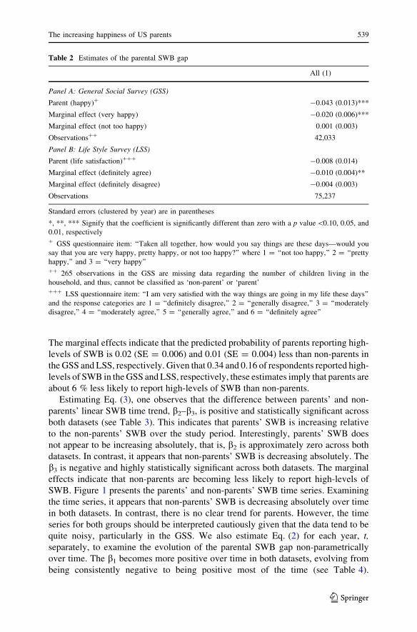
The marginal effects indicate that the predicted probability of parents reporting high-

levels of SWB is 0.02 (SE = 0.006) and 0.01 (SE = 0.004) less than non-parents in

the GSS and LSS, respectively. Given that 0.34 and 0.16 of respondents reported high-

levels of SWB in the GSS and LSS, respectively, these estimates imply that parents are

about 6 % less likely to report high-levels of SWB than non-parents.

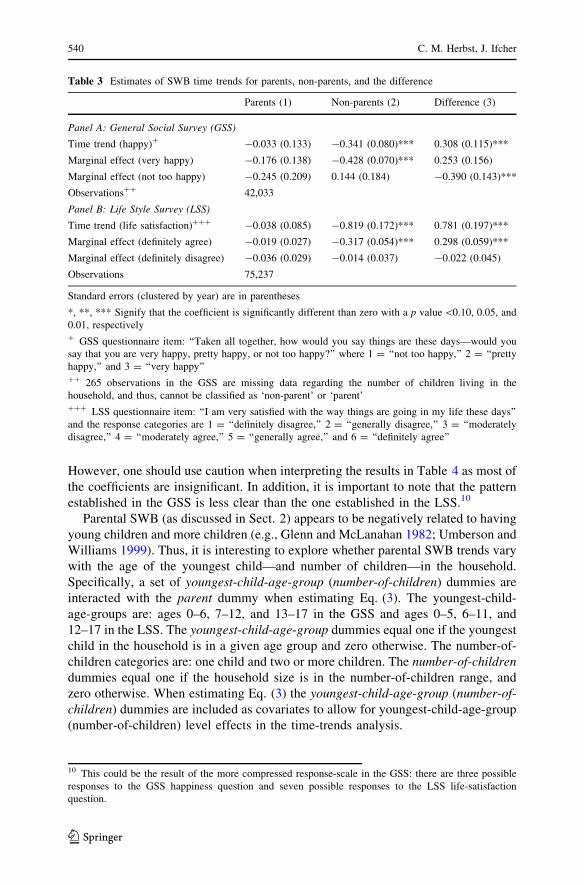
Estimating Eq. (3), one observes that the difference between parents’ and non-

parents’ linear SWB time trend, b2–b3, is positive and statistically significant across

both datasets (see Table 3). This indicates that parents’ SWB is increasing relative

to the non-parents’ SWB over the study period. Interestingly, parents’ SWB does

not appear to be increasing absolutely, that is, b2 is approximately zero across both

datasets. In contrast, it appears that non-parents’ SWB is decreasing absolutely. The

b3 is negative and highly statistically significant across both datasets. The marginal

effects indicate that non-parents are becoming less likely to report high-levels of

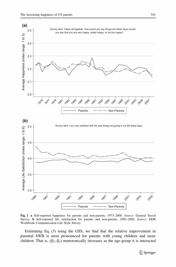
SWB. Figure 1 presents the parents’ and non-parents’ SWB time series. Examining

the time series, it appears that non-parents’ SWB is decreasing absolutely over time

in both datasets. In contrast, there is no clear trend for parents. However, the time

series for both groups should be interpreted cautiously given that the data tend to be

quite noisy, particularly in the GSS. We also estimate Eq. (2) for each year, t,

separately, to examine the evolution of the parental SWB gap non-parametrically

over time. The b1 becomes more positive over time in both datasets, evolving from

being consistently negative to being positive most of the time (see Table 4).

Table 2 Estimates of the parental SWB gap

All (1)

Panel A: General Social Survey (GSS)

Parent (happy)? -0.043 (0.013)***

Marginal effect (very happy) -0.020 (0.006)***

Marginal effect (not too happy) 0.001 (0.003)

Observations?? 42,033

Panel B: Life Style Survey (LSS)

Parent (life satisfaction)??? -0.008 (0.014)

Marginal effect (definitely agree) -0.010 (0.004)**

Marginal effect (definitely disagree) -0.004 (0.003)

Observations 75,237


*, **, *** Signify that the coefficient is significantly different than zero with a p value\0.10, 0.05, and

0.01, respectively? GSS questionnaire item: ‘‘Taken all together, how would you say things are these days—would you


happy,’’ and 3 = ‘‘very happy’’?? 265 observations in the GSS are missing data regarding the number of children living in the

household, and thus, cannot be classified as ‘non-parent’ or ‘parent’??? LSS questionnaire item: ‘‘I am very satisfied with the way things are going in my life these days’’

and the response categories are 1 = ‘‘definitely disagree,’’ 2 = ‘‘generally disagree,’’ 3 = ‘‘moderately

disagree,’’ 4 = ‘‘moderately agree,’’ 5 = ‘‘generally agree,’’ and 6 = ‘‘definitely agree’’


123

However, one should use caution when interpreting the results in Table 4 as most of

the coefficients are insignificant. In addition, it is important to note that the pattern

established in the GSS is less clear than the one established in the LSS.10

Parental SWB (as discussed in Sect. 2) appears to be negatively related to having

young children and more children (e.g., Glenn and McLanahan 1982; Umberson and

Williams 1999). Thus, it is interesting to explore whether parental SWB trends vary

with the age of the youngest child—and number of children—in the household.

Specifically, a set of youngest-child-age-group (number-of-children) dummies are

interacted with the parent dummy when estimating Eq. (3). The youngest-child-

age-groups are: ages 0–6, 7–12, and 13–17 in the GSS and ages 0–5, 6–11, and

12–17 in the LSS. The youngest-child-age-group dummies equal one if the youngest

child in the household is in a given age group and zero otherwise. The number-of-

children categories are: one child and two or more children. The number-of-children

dummies equal one if the household size is in the number-of-children range, and

zero otherwise. When estimating Eq. (3) the youngest-child-age-group (number-of-

children) dummies are included as covariates to allow for youngest-child-age-group

(number-of-children) level effects in the time-trends analysis.

Table 3 Estimates of SWB time trends for parents, non-parents, and the difference

Parents (1) Non-parents (2) Difference (3)


Time trend (happy)? -0.033 (0.133) -0.341 (0.080)*** 0.308 (0.115)***

Marginal effect (very happy) -0.176 (0.138) -0.428 (0.070)*** 0.253 (0.156)

Marginal effect (not too happy) -0.245 (0.209) 0.144 (0.184) -0.390 (0.143)***



Time trend (life satisfaction)??? -0.038 (0.085) -0.819 (0.172)*** 0.781 (0.197)***

Marginal effect (definitely agree) -0.019 (0.027) -0.317 (0.054)*** 0.298 (0.059)***

Marginal effect (definitely disagree) -0.036 (0.029) -0.014 (0.037) -0.022 (0.045)

Observations 75,237









10 This could be the result of the more compressed response-scale in the GSS: there are three possible

responses to the GSS happiness question and seven possible responses to the LSS life-satisfaction

question.


123

Estimating Eq. (3) using the GSS, we find that the relative improvement in

parental SWB is most pronounced for parents with young children and more

children. That is, (b2–b3) monotonically increases as the age-group it is interacted

2.0

2.1

2.2

2.3

2.4

2.5

Ave

rage

Hap

pine

ss (i

ndex

rang

e: 1

to 3

)

1975

1977

1979

1981

1983

1985

1987

1989

1991

1993

1995

1997

1999

2001

2003

2005

2007

Parents Non-Parents

Survey Item: Taken all together, how would you say things are these days–would

3.0

3.5

4.0

4.5

5.0

Ave

rage

Life

Sat

isfa

ctio

n (in

dex

rang

e: 1

to 6

)

1985

1987

1989

1991

1993

1995

1997

1999

2001

2003

2005

Parents Non-Parents

Survey Item: I am very satisfied with the way things are going in my life these days

you say that you are very happy, pretty happy, or not too happy?

(a)

(b)

Fig. 1 a Self-reported happiness for parents and non-parents, 1973–2008. Source: General SocialSurvey. b Self-reported life satisfaction for parents and non-parents, 1985–2005. Source: DDBWorldwide Communication Life Style Survey


123

with decreases, and it is larger when interacted with the two-or-more children

dummy than with the one-child dummy (see Table 5). Using the LSS, we find that

(b2–b3) is positive and statistically significant regardless of which age-group and

Table 4 Estimates of the parental SWB gap by year


1973 -0.037 (0.067) 1985 -0.196 (0.035)***

1974 -0.064 (0.068) 1986 -0.099 (0.035)***

1975 -0.116 (0.067)* 1987 -0.060 (0.034)*

1976 -0.001 (0.066) 1988 0.011 (0.034)

1977 -0.073 (0.066) 1989 -0.017 (0.035)

1978 -0.086 (0.062) 1990 -0.003 (0.035)

1980 -0.095 (0.074) 1991 -0.022 (0.035)

1982 -0.041 (0.068) 1992 -0.012 (0.035)

1983 -0.114 (0.063)* 1993 -0.027 (0.036)

1984 -0.127 (0.069)* 1994 -0.007 (0.035)

1986 -0.059 (0.092) 1995 0.024 (0.036)

1987 -0.129 (0.120) 1996 0.023 (0.035)

1988 -0.069 (0.066) 1997 0.008 (0.036)

1989 -0.117 (0.065)* 1998 0.000 (0.038)

1990 0.046 (0.069) 1999 -0.033 (0.038)

1991 -0.032 (0.067) 2000 -0.012 (0.039)

1993 -0.109 (0.062) 2001 0.082 (0.040)**

1994 -0.062 (0.047) 2002 0.050 (0.036)

1996 -0.027 (0.048) 2003 0.133 (0.040)***

1998 0.078 (0.048) 2004 0.034 (0.038)

2000 0.037 (0.048) 2005 0.077 (0.039)*

2002 0.006 (0.077)

2004 0.079 (0.078)

2006 -0.006 (0.052)

2008 -0.089 (0.065)





happy,’’ and 3 = ‘‘very happy.’’ LSS questionnaire item: ‘‘I am very satisfied with the way things are

going in my life these days’’ and the response categories are 1 = ‘‘definitely disagree,’’ 2 = ‘‘generally

disagree,’’ 3 = ‘‘moderately disagree,’’ 4 = ‘‘moderately agree,’’ 5 = ‘‘generally agree,’’ and

6 = ‘‘definitely agree’’?? For GSS the OECD equivalency scale was used where the first adult is equal to 1, additional adults

are equal to 0.5, and each child (under the age of 18) is equivalent to 0.3. For LSS first adult is equal to 1,

and additional household members are equal to 0.4 (LSS household size data does indicate the age of the

household members)??? 265 observations in the GSS are missing data regarding the number of children living in the

household, and thus, cannot be classified as ‘non-19ent’ or ‘19ent’


123

number-of-children dummy it is interacted with. That is, there is consistent evidence

that parents’ SWB is increasing relative to non-parents regardless of household

structure. In summary, there is no evidence that having younger children or more

children is associated with less relative improvement in parental SWB.

Parental SWB (as discussed in Sect. 2) is not a monolith. For example, female

parents worry more and experience lower levels of well-being than male parents

(Bird and Rogers 1998), and employed parents—especially working mothers—

experience lower mental health than unemployed childless adults (Simon 1998). To

investigate whether the trend of increasing relative parental SWB is widespread,

Eq. (3) is estimated for a series of relevant subgroups: men and women, employed

and unemployed adults, employed men and employed women, non-White and

White adults, and more and less educated adults. Results from the subgroup

Table 5 Estimates of SWB time trends by age of youngest child and number of children in the

household



Age of youngest child in HH

0–6 0.240 (0.179) -0.339 (0.080)*** 0.579 (0.147)***

7–12 -0.115 (0.096) 0.224 (0.124)*

13–17 -0.392 (0.252) -0.053 (8.000)

Number of children in HH

One -0.090 (0.171) -0.344 (0.079)*** 0.254 (0.161)

Two or more 0.024 (0.134) 0.368 (0.115)***



Age of youngest child in HH

0–5 -0.036 (0.092) -0.831 (0.172)*** 0.795 (0.211)***

6–11 -0.234 (0.156) 0.597 (0.245)**

12–17 -0.080 (0.132) 0.750 (0.180)***

Number of children in HH

One -0.182 (0.144) -0.826 (0.172)*** 0.645 (0.197)***

Two or more 0.082 (0.116) 0.908 (0.239)***

Observations 75,237


*, **, *** Signify that the coefficient is significantly different than zero with a p-value\0.10, 0.05, and








123

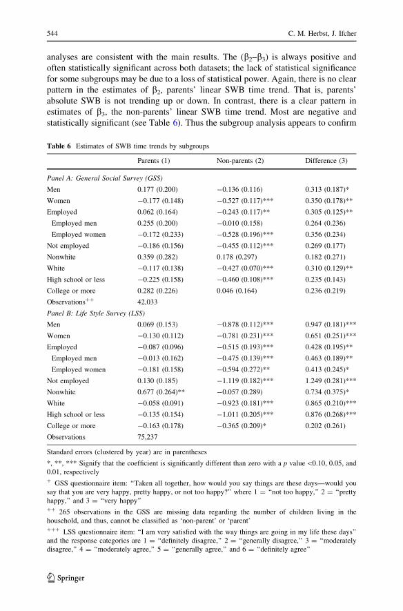
analyses are consistent with the main results. The (b2–b3) is always positive and

often statistically significant across both datasets; the lack of statistical significance

for some subgroups may be due to a loss of statistical power. Again, there is no clear

pattern in the estimates of b2, parents’ linear SWB time trend. That is, parents’

absolute SWB is not trending up or down. In contrast, there is a clear pattern in

estimates of b3, the non-parents’ linear SWB time trend. Most are negative and

statistically significant (see Table 6). Thus the subgroup analysis appears to confirm

Table 6 Estimates of SWB time trends by subgroups



Men 0.177 (0.200) -0.136 (0.116) 0.313 (0.187)*

Women -0.177 (0.148) -0.527 (0.117)*** 0.350 (0.178)**

Employed 0.062 (0.164) -0.243 (0.117)** 0.305 (0.125)**

Employed men 0.255 (0.200) -0.010 (0.158) 0.264 (0.236)

Employed women -0.172 (0.233) -0.528 (0.196)*** 0.356 (0.234)

Not employed -0.186 (0.156) -0.455 (0.112)*** 0.269 (0.177)

Nonwhite 0.359 (0.282) 0.178 (0.297) 0.182 (0.271)

White -0.117 (0.138) -0.427 (0.070)*** 0.310 (0.129)**

High school or less -0.225 (0.158) -0.460 (0.108)*** 0.235 (0.143)

College or more 0.282 (0.226) 0.046 (0.164) 0.236 (0.219)



Men 0.069 (0.153) -0.878 (0.112)*** 0.947 (0.181)***

Women -0.130 (0.112) -0.781 (0.231)*** 0.651 (0.251)***

Employed -0.087 (0.096) -0.515 (0.193)*** 0.428 (0.195)**

Employed men -0.013 (0.162) -0.475 (0.139)*** 0.463 (0.189)**

Employed women -0.181 (0.158) -0.594 (0.272)** 0.413 (0.245)*

Not employed 0.130 (0.185) -1.119 (0.182)*** 1.249 (0.281)***

Nonwhite 0.677 (0.264)** -0.057 (0.289) 0.734 (0.375)*

White -0.058 (0.091) -0.923 (0.181)*** 0.865 (0.210)***

High school or less -0.135 (0.154) -1.011 (0.205)*** 0.876 (0.268)***

College or more -0.163 (0.178) -0.365 (0.209)* 0.202 (0.261)

Observations 75,237










123

that parents’ SWB is increasing relative to non-parents’ SWB, and that non-parents’

SWB is decreasing absolutely.

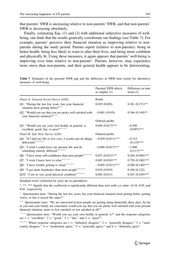
Finally, estimating Eqs. (1) and (2) with additional subjective measures of well-

being, one finds that the results generally corroborate our findings (see Table 7). For

example, parents’ perceive their financial situation as improving relative to non-

parents during the study period. Parents report (relative to non-parents): being in

better health, being less likely to want to alter their lives, and being more confident

and physically fit. Using these measures, it again appears that parents’ well-being is

improving over time relative to non-parents’. Parents, however, may experience

more stress than non-parents, and their general health appears to be deteriorating;

Table 7 Estimates of the parental SWB gap and the difference in SWB time trends for alternative

measures of well-being

Parental SWB deficit

or surplus (1)

Difference in time

trend (2)

Panel A: General Social Survey (GSS) Probit

Q1: ‘‘During the last few years, has your financial

situation been getting better?’’?0.019 (0.020) 0.381 (0.171)**

Q2: ‘‘Would you say that you are pretty well satisfied with

your financial situation?’’??-0.001 (0.019) 0.346 (0.149)**

Ordered probit

Q3: ‘‘Would you say your own health, in general, is

excellent, good, fair, or poor?’’???0.049 (0.017)*** -0.309

(0.097)***

Panel B: Life Style Survey (LSS) Ordered probit

Q4: ‘‘If I had my life to live over, I would sure do things

differently’’????-0.038 (0.011)*** -0.315

(0.119)***

Q5: ‘‘I wish I could leave my present life and do

something entirely different’’????-0.086 (0.017)*** -1.008

(0.117)***

Q6: ‘‘I have more self-confidence than most people’’???? 0.037 (0.012)*** 0.284 (0.098)***

Q7: ‘‘I wish I knew how to relax’’???? 0.045 (0.010)*** 0.720 (0.180)***

Q8: ‘‘I have trouble getting to sleep’’???? -0.092 (0.011)*** 0.500 (0.140)***

Q9: ‘‘I get more headaches than most people’’???? 0.010 (0.010) 0.160 (0.122)

Q10: ‘‘I am in very good physical condition’’???? 0.002 (0.013) 0.293 (0.109)***



0.01, respectively? Questionaire item: ‘‘During the last few years, has your financial situation been getting better, getting

worse, or has it stayed the same?’’?? Questionaire item: ‘‘We are interested in how people are getting along financially these days. So far

as you and your family are concerned, would you say that you are pretty well satisfied with your present

financial situation, more or less satisfied, or not satisfied at all?’’??? Questionaire item: ‘‘Would you say your own health, in general, is?’’ and the response categories

are 1 = ‘‘excellent,’’ 2 = ‘‘good,’’ 3 = ‘‘fair,’’ and 4 = ‘‘poor?’’???? Where response categories are 1 = ‘‘definitely disagree,’’ 2 = ‘‘generally disagree,’’ 3 = ‘‘mod-

erately disagree,’’ 4 = ‘‘moderately agree,’’ 5 = ‘‘generally agree,’’ and 6 = ‘‘definitely agree’’


123

they report (relative to non-parents) more headaches, difficulty relaxing, and trouble

falling asleep.

5 Discussion

The past few decades have witnessed a flurry of parental happiness research. Much

of this research finds that parents are less happy than non-parents. In this paper, we

critically assess this body of work and careful reexamine the relationship between

parental status and SWB, allowing the relationship to vary over time. Using two

nationally representative repeated cross-section surveys, we find evidence that

parents’ relative happiness is increasing over time, a finding that appears to be

driven by the absolute decline in non-parents’ happiness.

Our findings raise an interesting question: Why have parents experienced a

relative increase in happiness over the past few decades? We consider three

potential explanations. First, does having children protect parents against social and

economic factors that may be reducing well-being. Examples of such factors include

the decline in community and political involvement, growing disconnectedness

from family and friends, and the growth in economic insecurity. Indeed, many of

these themes are studied in Robert Putnam’s book Bowling Alone (2000). In

Putnam’s view, these changes are important because they have profound effects on

outcomes ranging from national economic prosperity and community health to

individual happiness. Added to these societal changes is the reported rise in

narcissism. In The Narcissism Epidemic (2009), Twenge and Campbell document

Americans’ increasing narcissism and its destructive effect on individuals and

society. Perhaps, parents are not as vulnerable to these changes, and as a result, have

been buffered against a decline in SWB. Indeed, previous research finds that one of

the benefits associated with parenthood is increased social connectedness (Gallagher

and Gerstel 2001; Nomaguchi and Milkie 2003).

To explore this possibility, we estimate parents and non-parents’ time-trends

replacing the dependent variables with measures organized around the themes of (1)

social and political connectedness, (2) social and political trust, (3) economic well-

being, and (4) balancing multiple responsibilities available in the LSS.

Consistent with Putnam’s (2000) work, Table 8 provides evidence in favor of the

steady erosion in Americans’ social and civic connectedness, interpersonal trust,

and economic security. Across virtually every measure, however, the reduction has

been substantially less dramatic among parents. Indeed, parents over time have

become relatively more likely to visit friends, to get the news every day, and to

remain engaged in politics. Interestingly, these relative improvements apply to the

economic realm as well: Parents are increasingly likely, relative to non-parents, to

agree that ‘‘family income is high enough to satisfy nearly all important desires,’’

and perhaps because of this, have become less likely to confide that ‘‘our family is

too heavily in debt.’’ Finally, even the indicator of balancing multiple responsi-

bilities favors parents. Parents and non-parents alike are increasingly likely to agree

with the statement ‘‘I feel like I am so busy trying to make everybody else happy

that I don’t have control of my own life,’’ but the upward trend among non-parents


123

has exceeded that among parents. Together, this evidence suggests that parents have

not experienced the growing social disconnectedness and economic insecurity to the

same extent as non-parents. Insofar as these social and economic factors are related

to SWB, such differential changes over time provide a plausible explanation for

why parents absolute SWB has not deteriorated, and has improved relative to non-

parents.

Second, it is possible that there has been a compositional shift in who is a parent,

and this has driven the observed relative increase in parental SWB.11 In other words, it

is not the impact of parental status on SWB that has changed over time; rather it is that

parents themselves are different. For example, the share of children living with one

parent rose from 14 % in 1970 to 25 % in 2008; the share of mothers with children

ages 17 and under in the labor force rose from 47 % in 1975 to 71 % in 2008; and the

average age of a women at the birth of her first child has risen from 21.4 years old in

1970 to 25 years old in 2006 (Pew 2010; Mathews and Hamilton 2009). Marital status,

employment status, and age are each well-known correlates of SWB. Further, more

Table 8 Estimates of SWB time trends for measures of social disconnectedness and economic insecurity


Panel A: social, civic, and political connectedness

‘‘I like to be considered a leader’’ -0.611 (0.128)*** -0.833 (0.118)*** 0.222 (0.094)**

‘‘I spend a lot of time visiting friends’’ 0.067 (0.088) -0.182 (0.096)* 0.249 (0.088)***

‘‘I need to get the news everyday’’ -1.733 (0.331)*** -2.468 (0.292)*** 0.735 (0.121)***

‘‘I am interested in politics’’ -1.139 (0.201)*** -1.329 (0.164)*** 0.190 (0.112)*

Panel B: social and political trust

‘‘Most people are honest’’ -1.622 (0.188)*** -1.638 (0.119)*** 0.016 (0.139)

‘‘An honest man cannot get elected to

high office’’

0.078 (0.134) 0.041 (0.103) 0.037 (0.061)

Panel C: economic well-being

‘‘It is hard to get a good job these

days’’

-0.800 (0.417)* -0.727 (0.550) -0.073 (0.179)

‘‘Our family income is high enough to

satisfy nearly all our important

desires’’

-0.544 (0.154)*** -1.207 (0.209)*** 0.663 (0.151)***

‘‘No matter how fast our income goes

up we never seem to get ahead’’

-0.514 (0.234)** 0.181 (0.261) -0.695 (0.304)**

‘‘Our family is too heavily in debt’’ 1.057 (0.217)*** 2.052 (0.165)*** -0.996 (0.142)***

Panel D: balancing multiple responsibilities

‘‘I feel like I am so busy trying to make

everybody else happy that I don’t

have control of my own life’’

0.626 (0.162)*** 1.079 (0.160)*** -0.453 (0.109)***



0.01, respectively

11 One potential explanation for the compositional changes in the population of parents and non-parents

is the second demographic transition.


123

women are choosing not to have children. The share of women ages 40–44 who had

never had a child rose from 10 % in 1976 to 20 % in 2006 (Blackstone and Stewart

2012). If adults feel freer, now than before, to choose to not be a parent, then the

observed relative increase in parental SWB might be due to better sorting of adults into

parents and non-parents. In summary, it is plausible that compositional shifts among

parents and non-parents have driven the change in parental SWB.

Third, it is possible that perceptions regarding gender roles and the division of

labor in the household, as well as the utility of marriage and children, have evolved

differently over time for parents and non-parents. This speaks not only to changes in

the selection into parenthood, but also to changes in views and behaviors within

marriage and parenthood that may influence SWB. Fortunately, the LSS contains a

rich set of questionnaire items that tap into such attitudes. We estimate parents and

non-parents’ time-trends replacing the dependent variables with various attitudinal

measures of gender, children, and marriage. Perhaps not surprisingly, parents

became more likely than non-parents to agree with the statement that ‘‘consideration

of the children should come first’’ when making family decisions. However, on a

number of other dimensions, parents and non-parents’ attitudes have evolved in a

similar manner. For example, both groups became equally more likely to agree that

‘‘couples should live together before getting married,’’ and equally less likely to

agree that the ‘‘father should be the boss in the house.’’ In addition, parents and non-

parents are no different in their evolving views on whether the ‘‘women’s liberation

movement is a good thing,’’ and they became equally disinclined to agree with the

view that a ‘‘woman’s place is in the home.’’ On balance, it appears that although

the characteristics of parents and non-parents have changed substantially over time,

changing views about women, marriage, and children have evolved similarly in both

groups. Thus, a tentative conclusion is that such views likely do not explain the

relative rise in parents’ SWB over the last few decades.

Although this paper does not answer the question as to the causal effect of

parenthood on happiness, one may infer from the results presented here that the

happiness ‘‘deficit’’ between US parents and non-parents has narrowed over time.

As pointed out by Kravdal (2014), there are significant challenges associated with

estimating the causal effect of parenthood. This paper—by showing trends in

happiness—focuses instead on presenting a series of stylized facts about the ways in

which parents’ and non-parents’ happiness has evolved over time. The paper also

advanced a number of plausible explanations for why parents experienced a relative

increase in happiness. Such findings may serve to catalyze future work in this area.

Acknowledgments We wish to thank seminar participants at the WEAI annual meeting (San Diego),

APPAM, and PAA as well as Rafael Di Tella, Richard Easterlin, Ori Heffetz, John Helliwell, Andrew

Oswald, Stephen Wu, and two anonymous referees for their helpful comments and suggestions. All

opinions and errors are those of the authors. The authors contributed equally to this work.

References

Aassve, A., Goisis, A., & Sironi, M. (2009). Happiness and childbearing across Europe. Working Paper

No. 10. Carlo F. Dondena Centre for Research on Social Dynamics.


123

Alesina, A., Di Tella, R., & McCulloch, R. (2004). Inequality and happiness: Are European and

Americans different? Journal of Public Economics, 88, 2009–2042.

Aneshensel, C. S., Frerichs, R. R., & Clark, V. A. (1981). Family roles and sex differences in depression.

Journal of Health and Social Behavior, 22, 379–393.

Barnett, R. C., & Baruch, G. K. (1985). Women’s involvement in multiple roles and psychological

distress. Journal of Personality and Social Psychology, 49, 135–145.

Bird, C., & Roger, M. (1998). Parenting and depression: The impact of the division of labor within

coupes and perceptions of equity. PSTC Working Paper No. 98-09. Population Studies and Training

Center. Providence, RI: Brown University.

Blackstone, A., & Stewart, M. D. (2012). Choosing to be childfree: Research on the decision not to

parent. Sociology Compass, 6(9), 718–727.

Blanchflower, D. (2008). International evidence on subjective well-being. NBER Working Paper No.

14318.

Blanchflower, D., & Oswald, A. (2004). Well-being over time in Britain and the USA. Journal of Public

Economics, 88, 1359–1386.

Clark, A. (2006). Born to be mild? Cohort effects don’t explain why well-being is U-shaped in age.

Working paper 2006-35, Paris-Jourdan Sciences Economiques.

Clark, A., Diener, E., Georgellis, Y., & Lucas, R. (2008a). Lags and leads in life satisfaction: A test of the

baseline hypothesis. The Economic Journal, 118, F222–F243.

Clark, A., Frijters, P., & Shields, M. (2008b). Relative income, happiness, and utility: An explanation for

the Easterlin paradox and other puzzles. Journal of Economic Literature, 46, 95–144.

Cleary, P. D., & Mechanic, D. (1983). Sex differences in psychological distress among married people.

Journal of Health and Social Behavior, 24, 111–121.

Di Tella, R., MacCulloch, R., & Oswald, A. J. (2001). Preferences over inflation and unemployment:

Evidence from surveys of happiness. American Economic Review, 91, 335–341.

Di Tella, R., MacCulloch, R., & Oswald, A. J. (2003). The macroeconomics of happiness. Review of

Economics and Statistics, 85, 809–827.

Dillman, D., Sangster, R., Tarnai, J., & Rockwood, T. (1996). Understanding differences in people’s

answers to telephone and mail surveys. New Directions for Evaluation, 70, 45–61.

Dolan, P., Peasgood, T., & White, M. (2008). Do we really know what makes us happy? A review of the

economic literature on the factors associated with subjective well-being. Journal of Economic

Psychology, 29, 94–122.

Evenson, R., & Simon, R. (2005). Clarifying the relationship between parenthood and depression. Journal

of Health and Social Behavior, 46, 341–358.

Frey, B., & Stutzer, A. (2006). Does marriage make people happy or do happy people get married? The

Journal of Socio-Economics, 35, 326–347.

Gallagher, S. K., & Gerstel, N. (2001). Connections and constraints: The effects of children on

caregiving. Journal of Marriage and the Family, 63, 265–275.

Glenn, N. D., & McLanahan, S. (1981). The effects of children on the psychological well-being of older

adults. Journal of Marriage and the Family, 43, 409–421.

Glenn, N. D., & McLanahan, S. (1982). Children and marital happiness: A further specification of the

relationship. Journal of Marriage and the Family, 44, 63–72.

Glenn, N. D., & Weaver, C. (1978). A multi-variate, multisurvey study of marital happiness. Journal of

Marriage and Family, 40, 269–281.

Glenn, N. D., & Weaver, C. (1979). A note on family situation and global happiness. Social Forces, 57,

269–282.

Gore, S., & Mangione, T. W. (1983). Social roles, sex roles, and psychological distress: Additive and

interactive models of sex differences. Journal of Health and Social Behavior, 24, 300–312.

Groeneman, S. (1994). Multi-purpose household panels and general samples: How similar and how

different? Paper presented at the Annual Meeting of the American Association for Public opinion

Research. Danvers, MA.

Grossbard, S., & Mukhopadhyay, S. (2013). Children, spousal love, and happiness: An economic

analysis. Review of Economics of the Household, 11, 447–467.

Hagstrom, P., & Wu, S. (2014 onlinefirst). Are pregnant women happier? Racial and ethnic differences in

the relatipnship between pregnancy and life satisfaction in the United States. Review of Economics

of the Household.

Hansen, T. (2011). Parenthood and happiness: A review of folk theories versus empirical evidence. Social

Indicators Research, 123, 1–36.


123

Hansen, T., Slagsvold, B., & Moun, T. (2009). Childlessness and psychological well-being in midlife and

old age: An examination of parental status effects across a range of outcomes. Social Indicators

Research, 94, 343–362.

Helliwell, J., & Wang, S. (2011). Weekends and subjective well-being. NBER Working Paper No. 17180.

Herbst, C. M. (2011). ‘Paradoxical’ decline? Another look at the relative reduction in women’s happiness.

Journal of Economic Psychology, 32, 773–788.

Herbst, C. M. (2012). Footloose and fancy free? Two decades of single mothers’ subjective well-being.

Social Service Review, 86, 189–222.

Ifcher, J., & Zarghamee, H. (2014). Trends in the happiness of single mothers: Evidence from the General

Social Survey. Journal of Happiness Studies, 15, 1219–1238.

Kahneman, D., Krueger, A., Schkade, D., Schwarz, N., & Stone, A. (2004). A survey method for

characterizing daily life experience: The day reconstruction method. Science, 306, 1776–1780.

Kohler, H.-P., Behrman, J., & Skytthe, A. (2005). Partner ? children = happiness? The effects of

partnerships and fertility on well-being. Population and Development Review, 31, 407–445.

Koropeckyj-Cox, T., & Call, V. R. (2007). Characteristics of older childless persons and parents cross-

national comparisons. Journal of Family Issues, 28, 1362–1414.

Kravdal, Ø. (2014). The estimation of fertility effects on happiness: Even more difficult than usually

acknowledged. European Journal of Population, 30, 263–290.

Lavee, Y., Sharlin, S., & Katz, R. (1996). The effect of parenting stress on marital quality: An integrated

mother–father model. Journal of Family Issues, 17, 114–135.

MacDermid, S. M., Huston, T. L., & McHale, S. M. (1990). Changes in marriage associated with the

transition to parenthood: Individual differences as a function of sex-role attitudes and changes in the

division of household labor. Journal of Marriage and the Family, 52, 475–486.

Margolis, R., & Myrskyla, M. (2011). A global perspective on happiness and fertility. Population and

Development Review, 37, 29–56.

Mathews T. J., & Hamilton B. E. (2009). Delayed childbearing: More women are having their first child

later in life. NCHS data brief, no 21. Hyattsville, MD: National Center for Health Statistics.

McLanahan, S., & Adams, J. (1987). Parenthood and psychological well-being. Annual Review of

Sociology, 13, 237–257.

McLanahan, S., & Adams, J. (1989). The effects of children on adults’ psychological well-being:

1957–1976. Social Forces, 68, 124–146.

Menaghan, E. (1982). Assessing the impact of family transitions on marital experience. In H.

I. McCubbin, A. E. Cauble, & J. M. Patterson (Eds.), Family stress, coping, and social support (pp.

90–108). Springfield, IL: Charles C. Thomas.

Myrskyla, M., & Margolis, R. (2014). Happiness: Before and after the kids. Demography, 51, 1843–1866.

Nomaguchi, K., & Milkie, M. (2003). Costs and rewards of children: The effects of becoming a parent on

adults’ lives. Journal of Marriage and the Family, 65, 356–374.

Pearlin, L. (1974). Sex roles and depression. In N. Datan & L. Ginsberg (Eds.), Life span developmental

psychology: Normative life crises (pp. 191–207). New York, NY: Academic Press.

Pew Research Center. (2010). The decline of marriage and rise of new families. Washington, DC: Pew

Research Center.

Putnam, R. D. (2000). Bowling alone: The collapse and revival of American community. New York, NY:

Simon and Schuster.

Putnam, R., & Yonish, S. (1999). How important is response rate? An evaluation of a ‘‘mail panel’’

survey archive. Working Paper. Cambridge: MA: JFK School of Government, Harvard University.

Ross, C. E., & Huber, J. (1985). Hardship and depression. Journal of Health and Social Behavior, 26,

312–327.

Ross, C. E., Mirowsky, J., & Goldsteen, K. (1990). The impact of the family on health: The decade in

review. Journal of Marriage and the Family, 52, 1059–1078.

Schuman, H., & Presser, S. (1981). Questions and answers in attitude surveys: Experiments on question

form, wording, and context. New York, NY: Academic Press.

Simon, R. W. (1998). Assessing sex differences in vulnerability among employed parents: The

importance of marital status. Journal of Health and Social Behavior, 39, 38–54.

Sousa-Poza, A., & Sousa-Poza, A. A. (2003). Gender differences in job satisfaction in Great Britain,

1991-2000: Permanent or transitory? Applied Economics Letters, 10, 691–694.

Stanca, L. (2012). Suffer the little children: Measuring the effect of parenthood on well-being worldwide.

Journal of Economic Behavior & Organization, 81, 742–750.


123

Stevenson, B., & Wolfers, J. (2008). Happiness inequality in the United States. Journal of Legal Studies,

37, S33–S79.

Stevenson, B., & Wolfers, J. (2009). The paradox of declining female happiness. American Economic

Journal: Economic Policy, 1, 190–225.

Stevenson, B., & Wolfers, J. (2010). Subjective and objective indicators of racial progress. Working

paper.

Twenge, J., & Campbell, W. K. (2009). The Narcissism Epidemic. New York, NY: Free Press.

Umberson, D., & Gove, W. (1989). Parenthood and psychological well-being: Theory, measurement, and

stage in the family life course. Journal of Family Issues, 10, 440–462.

Umberson, D., & Williams, K. (1999). Family Status and mental health. In C. S. Aneshensel & J.

C. Phelan (Eds.), Handbook of the sociology of mental health (pp. 225–253). New York, NY:

Kluwer Academic/Plenum.


123

The increasing happiness of US parents - Chris M....

Documents

Transcript of The increasing happiness of US parents - Chris M....