1

The Impact of Trade Liberalization on Revenue Mobilization and Stability in

Sudan1

Researcher Kabbashi Medani Suliman*

Institution University of Khartoum

Faculty of Economic and Social Studies Department of Economics

Khartoum, P.O. Box 321Sudan (Tel. 00249-83-769262)

* I wish to thank the GDN for the research grant under the ‘Macroeconomic Policy Challenges of Low Income Countries’ project. I would like also to thank Professor Peter Warr, the external reviewer who follows this study, for his comments at various stages of the preparation of the study and for his encouragements. Thanks are also due to Professor Gary McMahon who is with the administration of the project. I, however, remain solely responsible for the views expressed and for any remaining errors. 1 A revised report submitted to the: International Research Project on Macroeconomic Policy Challenges of Low Income Countries 2005 organized by the GDN.

2

Contents Executive Summary 4 I. Introduction

6

II. Background and Justification II.I. Background II.II. Justification of the Study

6 6 15

III. Conceptual Framework

15

IV. The Methodology

16

V. Estimation Results and Discussion VI. Conclusion References Appendixes List of tables:

Table (1): Selected macroeconomic indicators of the Sudanese Economy: sub-periods averages over (1970-2002) in percentages

Table (2): Indicators of the Sudanese Government Budget for Selected Years over 1970/71-2002 (in percentage share in GDP) Table (3): Tax revenue in Percent of the GDP in Some African Countries for Selected Years Table (4); The Contribution of the Main Taxes in Percent of the Total Tax Revenue (in Percentage of the Total Tax Revenue) Table (5): Selected Indicators of the Importance of Customs Revenues Table (6): Estimates of Tax Buoyancy in Sudan 1970-2002 Table (7): Comparison of Tax buoyancies over 1970-91 and 1992-2002 Table (8): The decomposed Tax Buoyancies Over the Reform and Pre-Reform Periods Table (9): Estimates of Tax Elasticity in Sudan 1970-2002 Table (10): Comparison of Nominal Measures of Tax buoyancy and Elasticity Over 1970-2002 Table (10’): Comparison of Real Measures of Tax buoyancy and Elasticity Over 1970-2002

Table (11): ADF Unit Root Test Statistics Table (12): Estimates of the Currency Ratio Equations Table (13): Estimate of the Size of the Underground Economy Using Tanzi’s Approach (in Million Sudanese Pounds Table (14): Estimate of the Size of the Underground Economy Using

22 40 41 44-52 7 10 11 13 15 23 24 25 28 29 29 30 31 33

3

Guttman’s Approach (in Million Sudanese Pounds Table (15): Estimates of Tax Evasion (in Millions Sudanese Pounds) Table (16): Cross-Correlations Between Non-agricultural GDP and the Main Fiscal Variables for Sudan

List of Figures

Figure (1): Real Revenue and Expenditure in Sudan Figure (2): Real Economic, Social and Other expenditures in Sudan Figure (3): The Development of the Major Tax Rates in Sudan

34 36 38 10 11 14

4

Executive Summary This study examines the buoyancy and the elasticity of the Sudanese tax system paying particular attention to the impact of trade liberalization on revenue mobilization and the stabilization role of the fiscal sector. The liberalization reform of 1992 was comprehensive. Its main objectives as far as the fiscal sector is concerned were to improve the incentive system and to enhance the tax yield and equity as well as to liberalize trade. The expectations were that the reform would increase the level of investment and income growth and hence broaden the tax base. The results of the analysis over 1970-2002 reveal that the tax system as a whole is not buoyant or elastic; the same results were also obtained for the major tax handles, namely; income and profit taxes, import duties and excise tax. In order to compare the performance of the tax system before and after liberalization, estimates of the nominal measures of tax buoyancy were carried over 1970-91 and 1992-2002. The results show that for total tax revenue, income tax, profit tax and excise tax, the direction of changes of tax buoyancy is difficult to ascertain. However in the case of import duties the estimates suggest that buoyancy improved after the reform. Real measures of buoyancy and elasticity confirm this general results and indicate that the composition of total tax is skewed away from trade and income taxes towards domestic indirect tax. The comparison of the decomposed buoyancies of nominal taxes to their respective bases (tax-to-base elasticity) and elasticities of the nominal bases to income (base-to-income elasticity) reveals that the base to income elasticity seems to be growing for business profit personal income taxes. The elasticity of tax-to-base is low for almost all the major tax handles in the country over the reform period implying that tax collection has not increased in proportion to the growth in tax bases reflecting the combined effects of tax evasion, administrative inefficacy, tax exemptions, complexity of the tax system, corruption and slacks in enforcement of law. Comparison of buoyancy and elasticity over the review period indicates that tax yield from import duties has improved as a result of the various tax discretionary changes. However, in the case of other major taxes firm conclusions cannot be drawn. Tanzi’s approach is used to estimate the magnitude of tax evasion in the country. The results of the calculations reveal that tax evasion is substantial and growing over time due to the growth of the underground economy and the relatively high average tax rate. Average tax evasion, over the review period, stands at about 53 percent of actual tax yield and 33 percent of the potential tax yield inclusive of the underground economy’s GDP. This implies that tax reform through rate reduction alone may not be enough to check the growth of the underground economy. Such effort should be part of a policy reform that aims at removing the remaining controls and barriers to entry into the formal economy including the reform of the tax administration system and the simplification of its complexities. Checking of black and parallel markets activities demands enforcement of the law and accountability of officials.

5

Further evidence on the effect of removing controls, through liberalization, is obtained by estimating the determinants of trade revenue proxied by import duties, which is the main tax handle of the system. The estimates suggest that the trade tax yield improved due to an increase in the volume and value of imports relative to GDP, as a result of liberalization. However, because high tariff is an important determinant of trade revenue, the marginal benefit of tax evasion is still considerable. The assessment of the stability attributes of the fiscal sector shows that the relatively low buoyancy and elasticity of the tax system negatively impact the work of build-in-stabilizers and hence amplify the macro fluctuations over the course of the business cycle. This impact of the budget outcome must be acknowledged and accounted for when analyzing fiscal trends in Sudan. The use of the cyclically adjusted fiscal indicators can improve the efficiency of decision-making in the country and enhance the macroeconomic stabilization role of the tax system. More important the dismal performance of the tax system provide explanation for the low tax efforts and the relatively low and declining government spending; which in turn implies negligence of the productive sectors of the economy. In this context, there is a considerable danger that, the rise in windfalls associated with the recent boom in the oil sector, may provide lack of incentive to develop alternative tax bases and/or improve the existing ones, with the obvious result of reducing public accountability, inducing destructive rent seeking activities and an efficient allocation of the resources in the economy

6

I. Introduction

A traditional function of the tax system is to bring in sufficient revenue to meet the growing public sector requirements. Common measures of the ability of the tax system to mobilize revenues are buoyancy and elasticity (Asher 1989). In general the growth of tax in response, for example to GDP, can be decomposed into automatic growth, due to an increase in the base on which tax is charged, and growth resulting from discretionary changes in tax rates and legislations. A desirable property of a tax system is that income elasticity be equal or greater than unity. Such property ensures that revenue growth keeps pace with that of GDP without frequent discretionary changes. More important, it imparts automaticity, or build-in stability, to the tax system. And hence, ensures mitigation of cyclical variations in GDP over the course of the business cycle. Low tax buoyancy and elasticity can be attributed to many factors. Important among these are tax evasion and low compliance resulting mainly from inefficient tax administration, corruption and high tax rates. The purpose of this study is to examine the buoyancy and elasticity of the Sudanese tax system and to assess the impact of the recent trade liberalization on revenue mobilization. The stabilization role of the main fiscal variable is also evaluated. Lessons from other experiences, through useful, may not contain full answer to the needs of a given country, ‘when it comes to taxation each country is, or feels that it is unique’2. In theory the direction of changes in revenues as a result of trade liberalization is ambiguous depending inter alia on revenue productivity and tax structure. The specific objectives to be addressed are four fold. First, to estimate tax buoyancy and elasticity of the Sudanese tax system as a whole, then evaluate the response of this system to trade liberalization in 1992. Second to evaluate the extent to which the 1992 liberalization reform enhanced the capture of evaded tax. Third, to look at the stability attributes of the main fiscal variables in the country and to indicate their macroeconomic implications. Finally, to provide a discussion on a tax reform that could help in augmenting the revenue mobilization ability of the Sudanese tax system. II. Background and Justification II.I. Background II.1.1. An Overview of Economic Performance Sudan is endowed with considerable natural resources, by Sub-Saharan African countries’ standards, including large and rich agricultural land, as well as petroleum and natural gas reserves. However the performance of the country in many ways typifies the severe economic decline that has affected many countries in the region since the 1970s.

2 Tanzi (2003, P 9).

7

Sudan’s real GDP grew at 1.1% if the annual percentage growth rate is used (see table 1 last row). As seen in this table the annual percentage growth rate of real GDP suggests that there were two periods of positive economic growth over the review period during 1971-83 and in the 1990s. Over the first period peace prevailed (1972-83), however, the government policies were not growth oriented. The inflow of capital over this period compensated for the relatively low ratio of investment to GDP of 12.94% over this sub-period as well as for the poor performance of exports relative to imports. The nominal period average growth rates of both were about 7.5% and 14.3% respectively (see table 1). However, a substantial share of capital inflow was channeled to finance the state-led development venture, which resulted in the establishment of a number of large and loss-making public enterprises. The result was a rapid accumulation of external debts and arrears to the extent that Sudan was declared ineligible to use the IMF’s general resources in 1986 (see World Bank Country Economic Memorandum 1990).

Table (1): Selected macroeconomic indicators of the Sudanese Economy: sub-periods averages over (1970-2002) in percentages

Sub-Period Real GDP Growth (%)

Consumer Price Inflation (%)

Ratio of Fiscal Deficit to GDP (%)

Nominal Imports Growth/1

Nominal Exports Growth/1

The Ratio of Investment to GDP (%)

Ratio of Current Account to GDP (%)

Change in Free Nominal Exchange Rate (%) /2

Change in the Official Exchange Rate (%) /2

1971-1983 3.8 (2.06)

19.9 (0.50)

-7.67 (037)

14.3 (1.43)

7.47 (2.49)

12.94 (0.40)

-3.74 (0.71)

9.43 (12.16)

8.52 (1.63)

1984-1991 -2.50 (9.40)

55.6 (0.59)

-12.16 (0.39)

-1.44 (19.9)

-3.64 (9.03)

10.7 (0.37)

-1.22 (1.50)

78.11 (0.95)

30.1 (0.67)

1992-2002 7.90 (1.45)

57.9 (0.87)

-2.40 (0.86)

18.4 (1.82)

20.20 (23.06)

19.15 (0.30)

-7.73 (0.30)

39.26 (0.99)

137.10 (2.20)

1971-2002 3.70 (4.00)

41.90 (0.91)

-7.11 (0.69)

8.81 (2.51)

9.79 (3.16)

14.40 (0.42)

-4.39 (0.78)

36.89 (1.40)

58.10 (3.13)

Note: 1/Based on Export and import expressed in US dollar. 1/The parallel nominal and the official exchange rates are defined as the local currency per unit of the US dollar. Hence percentage growth implies depreciation. Source: Bank of Sudan Annual Reports, World tables and the IFS The sub-period 1984-91 showed a negative average real GDP growth of 2.5% , the period average nominal export rate declined by about 3.6% and the share of investment to the GDP declined by about 2.2 percentage points compared to its growth in the previous period. The main cause for this poor performance has been the outbreak of the civil war in 1983, the poor economic policies and the natural disasters such as drought over 1984-5 and flood in 1988. Nonetheless, the impact of the civil war was severe, in addition to its human costs; the war has disrupted development in the southern third of the country that has been the battlefield. Development in the rest of the country was affected as the war drained economic resources and manpower. The government expenditures were directed to finance the war, the loss-making public enterprises and the subsidies for urban consumers. In addition revenue effort has been declining due to the ill-advised tax policies e.g. the abolition of income tax over 1984-85, the poor administration of revenue collection and the inappropriate exchange and price policies. The fiscal deficit as a

8

percentage of the GDP grew by about 4.5 percentage points higher than its average growth over the peace period. The growing deficit was financed mainly through money printing as a result the economy was pushed into chronic inflation. The consumer price index (CPI) inflation grew by 55.6% period average rate. An entrenched system of price and exchange rate controls as well as import quotas was introduced in response to chronic inflation. This in turn fed into parallel and black markets as well as into rent seeking and corruption that nurture the spread of underground activities. Although import growth was compressed over this sub-period by about 15.7 percentage points compared to its average growth over the peace period, nominal export growth declined over the period making it difficult to reverse the current account deficit. The poor performance of export was caused by excessive licensing requirements, over regulation of the irrigated agriculture-- the provider of the main export crops-- inefficient state parastatals in charge of export marketing and the overvaluation of the official exchange rate-- often used in export valuation-- compared to the free market determined rate (see table 1). Investment over this period has been set back by a cumbersome investment regulation and the by channeling of the already meager domestic credit to the inefficient public enterprises. Over the second period of economic growth, over 1992-2002, the government pursued a macroeconomic stabilization programme, the main elements of this reform involving abolition of price and quotas controls, consumer subsidies, privatization of the loss-making public enterprises and devaluation of the official exchange rate. As seen in table (1) the official exchange rate has been devalued by 107 percentage points compared to its average growth rate over the pervious period. As a result nominal export excluding oil reversed its declining trend to grow by a 22.2% period average annual rate. In addition to the implementation of the reform, the years of good weather favoured agricultural growth and the boom in oil and oil related industries and services has also positively impacted the GDP growth as the investment to GDP ratio grew on average by about 19.2% over this period. From this brief review of economic performance it appears that, as disruptive as the natural disasters and the civil war have been to the economy, there are important aspects of economic decline that they cannot explain3. The poor economic performance over 1984-1991 compared with the sub-period 1992-2002 suggests that the ill-advised policies and the government approach to policy making played an important role. Thus while peace is a necessary condition for economic growth it is by no means sufficient for the realization of this objective. Hence, as the growth experience of the post 1992 reform showed, in addition to peace a firm commitment to a credible stabilization programme is needed. Furthermore to ensure that economic growth is sustainable in the long run, commitment to the stabilization reform has to be supported by inflow of generous foreign assistance, debt forgiveness and debt rescheduling on soft terms and the government should take measures to address the remaining supply constraints. 3 See also the World Bank Country Economic Memorandum (1991 and 2003)

9

II.1.II. The Fiscal Profile At political independence in 1956 Sudan inherited a rudimentary tax system. The colonialists, aside from business profit tax, relied on haphazard traditional taxes levied on land, animals and fruit trees4. However, since the 1970s the Sudanese tax system had undergone a number of individual tax adjustments and major reforms in response to the growing public sector expenditure requirements and for improving the incentive structure in order to achieve development goals normatively defined. The most notable reforms were taken in 1987 and 1992, both reforms were undertaken by the taxation section of the Ministry of Finance and National Planning The two reforms emphasized the following: first, the enhancement of tax administration and the efficiency of the tax system with a view to improve revenue yield and to ensure equity. Second the reduction of the number of steps on income tax and pushing up of the exemption income for married persons in the range of 35 –50 percent compared to unmarried people. Third the gradual shift from trade-based tax to taxation of domestic production. The generalization of the excise and sale taxes as broad base indirect taxes. Despite these reforms and the various adjustments of the individual taxes, the Sudanese tax system appears less productive. A look at the fiscal structure reveals a number of aspects: first, the revenues and expenditures shares in the gross domestic product (GDP) declined from 24% and 31% in 1970 to 12.4% and 13.5% in 2002 respectively, these latter shares are almost half their respective levels in 1970, (see table 2 below). The plot of real total tax revenue and expenditure shows a declining trend for real revenue from 1970 to about 1981, then over 1982-83 real revenue increased, but has since then declined. Real total expenditure showed no clear trend from 1970 up to mid 1990s with the exception of a pike in 1989, the then declined to its 1970s level (see figure 1). The performance of the major components of public expenditures is not better, for example, the real expenditures on both social and economic services seem to decline over the review period except for the spikes in 1978, 1988 and 1995 (see figure 2). Table (2) reveals that tax effort, or tax burden, measured by tax/GDP ratio declined from 15.1% in 1970 to 5.9% in 2002 and averaged 11.5%. Compared with a sample of other African countries, the Sudanese tax effort was less than the average of the sampled countries. Sierra Leone and Burundi are the only countries that compare with Sudan (see table 3).

4 No attempt was made during the colonial period to introduce an “appropriate” tax system for Sudan. The main reason seems to have been the conviction of the colonialists that the Sudanese were not tax minded. More important raising taxes was thought unwise since it had been one of the factors that let to the Mahadist Revolution that ousted the Ottoman rule in Sudan in the late 19th century (see Nimeiri 1974).

10

Table (2): Indicators of the Sudanese Government Budget for Selected Years over

1970/71-2002 (in percentage share in GDP)

1970/1-74/5 1975/6-80/1 1981/2-1984/5 1985/6-89/90 1991/2-1994/5 1996-2000 2002

Total Revenue Tax revenue Oil revenue Total expenditures/a Overall Cash Deficit Financing External Internal

24.0 19.1 11.4 8.8 7.3 8.0 12.4 15.1 11.1 9.7 6.3 5.5 5.8 5.9 00 00 00 00 00 1.0 5.8 31.0 26.9 21.3 21.4 13.9 8.9 13.5 -7.0 -7.8 -9.9 -12.6 -6.6 -0.9 -1.1 4.9 5.2 7.8 6.7 2.7 0.3 0.1 2.1 2.6 1.8 5.6 4.0 0.6 1.0

a/ Excluding interest arrears. Source: Ministry of Finance and National Economy

Figure (1): Real Revenue and Expenditure in Sudan

050

100150200250300350400

1970

1972

1974

1976

1978

1980

1982

1984

1986

1988

1990

1992

1994

1996

1998

2000

2002

In M

illio

n Su

dane

se p

ound

s

Real expenditure Real revenue

11

Figure (2): Real Economic, Social and Other expenditures in Sudan,

0

10

20

30

40

50

60

1970

1972

1974

1976

1978

1980

1982

1984

1986

1988

1990

1992

1994

1996

1998

2000

2002

Econ

omic

and

soci

al e

xpen

ditu

re (I

n M

illio

n Su

dans

es P

ound

s)

0

50

100

150

200

250

300

350

Oth

er e

xpen

ditu

re (I

n m

illio

n Su

dane

se

poun

ds)

Economic Services Social service Other expenditure

Table (3): Tax revenue in Percent of the GDP in Some African Countries for

Selected Years. 1980 1985 1990 1991 1992 1993 1994 1995 Gambia 19.9 15.6 18.5 20.4 21.8 22.02 17.4 - Burundi 12.6 - 10.2 10.1 8.7 9.3 10.0 11.0 Sierra Leone 14.8 5.4 9.6 11.7 13.3 13.9 10.1 9.2 Botswana 24.9 23.0 28.6 36.9 39.9 33.1 28.9 27.0 Malawi 16.2 18.3 19.2 16.3 15.5 14.8 14.5 15.3 Kenya 21.1 18.8 19.3 19.8 20.0 24.5 24.4 25.9 Sudan 11.4 10.8 8.7 11.0 15.1 10.2 12.4 11.5 Sample average 17.3 15.3 13.9 18.02 19.2 18.3 16.8 16.7 Source: UNPAD and Stotsky and Woldemariam (1997)

Second, The Sudanese tax system seems to fail to mobilize enough revenue to finance the requirement of the public sector and development. The budget deficit has been growing especially over 1980-1990 (see table 1 and 2). Chronic deficit, in theory, has implications for a) the balance of payments, if financed though foreign borrowing, b) the cost of finance and private investment, if financed through domestic borrowing and c) inflation,

12

if financed through money printing A combination of these methods were used at various degree in financing the fiscal deficit in Sudan over the review period.

Foreign borrowing was an important source of finance over 1970-1989. Although foreign borrowing raises indebtness and future debit servicing obligations it is less inflationary. However, this source has dried up since late 1989 for Sudan. Accordingly the government resorted to domestic borrowing mainly from the banking system. As a result money supply increased rapidly fueling the severe inflationary pressures that pushed the economy into chronic inflation by the dawn of the 1990s. Attempts to repress inflation through import and price controls as well as through administrative measures add further to setbacks in public policy. The control policy resulted in entrenched smuggling and rent seeking, it also gave rise to black and parallel markets that fed into inflation. In particular the control of foreign exchange created a lucrative parallel market for foreign exchange that in turn resulted in overvaluation of the official exchange rate. These policy-induced distortions discourage the incentives for production, and internal and external trade. Neither foreign loans nor borrowing from the domestic banking system can be relied on as sustainable sources of financing in Sudan. In view of the problems associated with these sources raising of additional funds must rest with the tax system. A third feature of the Sudanese fiscal structure is the heavy reliance on indirect tax, especially foreign tax, as the main source of revenues. However, from table (4) below, it appears that indirect tax has declined by about 10% over 1980-85, but it increased again over 1996-2002 implying that this decline is not associated with a major change in the tax structure. It is evident from the table that commodity taxation dominated the Sudanese tax structure. The share of import tax was high. It contributed about 41% over the review period. The share of excise tax was 32.3% in total tax in 1970 and since then showed a declining trend up to the mid 1990s, where it started to increase again. Export duties and royalties accounted for a much smaller share of the total tax revenue averaging only 2.5% over the review period. The reason for this low contribution is that agricultural products up to 1999 dominated exports, where oil export became important afterwards. Generally tax levies on these products are low averaging about 5% ad valorem compared to average import duty rate of about 36% at valorem. Low export duties were followed to improve the competitive stand of cotton, which was the main export crop up to 1999. It seems that the Sudanese tax structure over the review period does not conform to the upheld scenario that economic development brings with it an increase in the share of direct tax in total revenue (see e.g. Musgrave 1969). Such profile of development is consistent with the experience of the developed economies in which direct tax mobilizes more revenues than the indirect tax. The implication of the inability of Sudanese tax system to replicate this pattern is that accurate tax revenue projection and targeting of

13

Table (4); The Contribution of the Main Taxes in Percent of the Total Tax Revenue (in Percentage of the Total Tax Revenue)

Year Indirect tax

Direct tax

Personal income tax

Business Profit tax

Export tax

Import tax

Excise Tax

1970 1971 1972 1973 1974 1975 1976 1977 1978 1979 1980-1985 1986-1990 1991-1995 1996-2002 1970-2002

85.4 84.8 84.6 83.9 84.8 85.9 85.2 85.6 84.9 83.0 72.6 78.6 65.9 75.0 76.7

14.6 15.2 15.4 16.1 15.2 14.1 14.8 14.4 15.1 17.0 27.4 21.4 34.1 25.0 23.3

3.8 3.5 3.4 3.5 2.6 3.1 3.5 3.6 4.1 6.0 5.9 4.4 7.7 6.0 5.3

8.6 9.0 8.7 9.2 8.2 10.8 8.6 8.7 10.2 9.7 12.7 13.6 24.1 15.1 14.0

4.7 5.3 4.4 5.8 4.1 5.1 4.3 4.1 4.4 3.8 2.2 1.4 0.99 1.6 2.5

45.7 42.0 31.1 40.2 28.3 45.1 39.4 42.2 56.4 44.1 51.4 52.1 25.6 32.6 40.9

32.3 29.6 27.4 29.7 20.5 18.9 27.8 23.9 21.7 21.2 14.9 14.6 18.6 23.7 19.9

Source: Ministry of Finance and National Economy and the Central Bureau of Statistics. specific tax revenue source cannot easily be made in the light of the upheld view of the fiscal profile as development unfolds. The worsening economic condition driven by the fiscal and other variables has generated a variety of response by individuals and the government. In response to the declining incomes resulting from inflation erosion, individuals adjusted their behaviour in search for better alternatives. Brown (1992) assessed the impact of three most prevalent and closely interrelated modes of individual responses on the exacerbation of the macro-imbalances and the growth of the hidden economy in Sudan over 1978-87. These were: international migration, the spread of the parallel market and capital flight. His analysis revealed that the revised macroeconomic aggregates incorporating unrecorded transactions associated with the hidden economy give a completely different picture of the nature of the macroeconomic imbalances in Sudan. Since late 1980 various official responses were made to the conditions of decline, however, the introduction of the Comprehensive National Salvation Strategy CNSS in 1992 was a notable attempt. As far as the macro and fiscal management component of the CNSS are concerned, the CNSS emphasized i) the reduction of the internal, fiscal, and the external, balance of payments deficits, through the unification of the exchange rate and the introduction of a strict cash budget system for fiscal control ii) liberalization of trade and the removal of administrative controls including reduction of trade tariffs, iii) achievement of price stability and iv) enhancement of economic growth. The achieved macro stability and inflation control under this programme, especially over the period

14

1996- 2004 involved severe retrenchment of public spending. It is known that at times of expenditure cut, public investment on health and education--which are among the most effective vehicles available for reaching the poor-- will be the first victim. Performance on this count falls short of the socially desired level. In this context the recent IPRSP (2004) noted that no effort are made to address the human development in the country and even doubted the ability of the government to fulfill the MDGs by 2015. Nonetheless, the liberalization of internal and external trade is expected to contribute to the dissolution of the parallel market phenomena and the associated harmful speculative and rent seeking behaviour. Hence, the flow of the unrecorded international financial transactions and the domestic transactions associated with the underground economy are expected to decline. Trade liberalization also facilitated Sudan’s accession to African and Arab regional groupings, in particular the COMESA (Common Market of Eastern and Southern Africa). For this purpose, import tariff reduction came a long way from 250%-45% range-- with complicated structure over the control period-- to three bands of 10%, 20% and 45% in 2002. Also all export tariffs were reduced from an average of 50%-20%, as in the pre-reform period, to 2% in the reform period, except the tariffs on raw leather and sesame oil which remain at 15% and 20% respectively. Preferential tariffs as well as zero tariffs were signed with some COMESA states members. Figure (3) shows the plot of the major tax rates in Sudan over the review period. As seen, of all tax charges, the tariff rate was the highest followed by the business profit tax, while excise and personal income charges remained low over the sample period. It also appears from the figure that all tax charges declined over the reform period.

Figure (3): The Developments of the Major Tax Rates in Sudan

01020304050607080

1970

1972

1974

1976

1978

1980

1982

1984

1986

1988

1990

1992

1994

1996

1998

2000

2002

In P

erce

ntag

e

Exice tax rate Income tax rate Profit tax rate Tariff rate

Table (5) shows the performance of exports, imports, and custom revenues for selected years over 1970-2002. As seen in the table imports share in the GDP, which is a measure of trade revenue base, is relatively stable while the total revenue share showed a declining trend throughout the review period. The share of trade revenue in total revenue is relatively high, however, it declined over 1991-95 to almost half its level in 1980s, but since then it increased and subsequently remained stable.

15

Table (5): Selected Indicators of the Importance of Customs Revenues in Sudan 1970-80 1981-90 1991-95 1996 1997 1998 1999 2000 2001 2002 Exports/GDP/a 13.8 6.6 0.41 4.9 5.1 5.1 7.6 16.1 13.7 13.3 Imports/GDP 15.2 10.7 22.1 16.5 13.5 16.3 12.1 11.8 15.6 14.6 TR/ TOTR/b 47.9 53.3 26.6 31.4 40.6 32.5 34.8 33.4 31.6 35.4 TR/GDP 7.1 5.8 3.2 1.9 2.1 1.9 2.2 1.8 1.8 2.0 a/Oil revenues are included as from 1999. b/ TR is the customs revenue; TOTR is the total tax revenue. Source: The Ministry of Finance and the National Economy. II. Justification of the Study As in other LDCs the fiscal sector in Sudan is the focal point of many of the conflicts and challenges posed by development. The resource mobilization for redistributive, allocative and stabilization functions of the government is seriously compromised by these challenges. As noted the fiscal performance over the 1970s and 1980s was discouraging. The response by individuals and by the government had created options and blocked others. The current government’s policy stand involves thorny compromises. In particular, Sudan subscribed and approved the MDGs as guidelines to its socio-economic development, which demand budget with a human face. However, progress on this count is not encouraging. One reason, as noted earlier, is that much of the recent macroeconomic stability is achieved through severe financial crunch especially from human development spending categories. Furthermore, the urgent needs of the post conflict period are expected to puts an added pressure on the fiscal sector to mobilize resources for rehabilitation of the economy and the society, while there are needs for Sudan to further reduce its tariff rates, which implies revenue loss, to access existing African and Arab regional grouping and eventually qualifies for joining the WTO. More important, most multilateral macro-policy documents on Sudan-- that in active use in the current policy dialogues-- emphasize the importance of the quality of tax administration system, and ensure that the decline in custom revenue as a result of liberalization will be matched mainly through administrative improvement. That said, there is no sound empirical base for directing such reforms. More important, to date there is no empirical study in Sudan on the assessment of the size of evaded tax and the extent to which the liberalization measures of 1992 has captured the unreported activities into the tax web. This study attempts to fill this gap in information by piecing together empirical evidence on some important aspects of the Sudanese tax system. It examines the elasticity of the tax system and its stabilization role as well as the extent of tax evasion and capture. III. Conceptual Framework High buoyancy and elasticity are desired attributes of a tax system, aside from augmenting the revenue productivity; they enhance the overall fiscal operations in mitigating undesired cyclical movements. Progressive income tax is an example of a

16

powerful automatic stabilizer. As income rises tax yield increases and falls more than proportionately when income declines. Expenditure-based tax may be less automatic and hence the anti-cyclical impact of consumption may tend to be less than income. Accordingly, the assessment of tax elasticity is an integral part of a macro model of any economy. It is important not only for examining the responsiveness of the tax system, but also for the evaluation of the system’s efficiency and equity aspects. Income elasticity of tax can be decomposed into tax-to-base and base-to-income elasticities. Knowledge of these components is important for policymaking; first it helps in identifying the source of either fast or lagging revenue growth, second it highlights the components of growth that are amenable to policy manipulation, e.g. tax base ratio is within the control of the policy maker while the base to income elasticity is not. One of the central problems that any tax administration encounters is cheating or evasion. High incidences of tax evasion5 relate to high tax rate, low probability of detection and low penalty for tax evasion. Tax evasion is usually associated with undervalued and officially unrecorded transactions, which relate to the so-called underground economy. Different writers have used different terms to describe such activities, e.g. informal, shadow, underground, second economy, subterranean or hidden economy. These different perceptions of the underground activities have given rise to differences in the perception of its legality. There are those who see the underground economy as dysfunctional phenomenon that denies the society its legal revenue, and there are those who view it as a creative adaptation to the failure of the formal economy to deliver the required goods and services in a timely manner (see e.g. Wile 1987 and Osoro 1993). In the Sudanese context, the underground economy is taken to mean all unregistered firms according to the Company Ordinance of 1925 that employ less than 25 workers, or have no license and regular tax payment records. If the underground economy is sizable and growing relative to the official economy, it will not only compromise the revenue mobilization ability of the tax system, but it also gives biased estimates of the coefficients of the fiscal variables. The extent of tax evasion is difficult to determine. An indirect method will be used to give an idea about tax evasion in Sudan. As will be indicated in the next section, two versions within the monetary approach were suggested to determine the size of the Sudanese underground economy. IV. The Methodology The main research questions to be addressed are: a) Which tax instrument in Sudan is more (less) responsive and how the tax system responded to the wave of trade

5 Tax evasion is the failure to pay a legally due tax, in contrast tax avoidance relates to the changes in agent’s behaviour in such a way to reduce legal tax liability.

17

liberalization of 1992?, b) Does the reform enhance the capture of evaded tax, and how does it affect the stability of the tax system?, c) What are the macroeconomic implications of (a) and (b)? Broadly speaking, an eclectic method of the before and after approach will be used to provide answers to these questions. Accordingly, the analysis will be carried out at three stages summarized as follows: At the first stage, the analysis starts with the evaluation of the overall productivity of the Sudanese tax system and its ability to mobilize revenues. Two measures are normally used in this evaluation. These are the buoyancy and elasticity of a given tax system. Buoyancy measures increases in tax revenue due to increase in income, combining the effects of expanding the base, e.g. by introducing a new tax, and enhancing the rates of existing taxes. Although tax measurements design to expand the base and/or augment tax rates permit the tax system to start at a high level, this is not a substitute for elasticity, which is essential for sustaining the cumulative process6 When no attempt is made to control for discretionary measures that alter the tax rate and/or base, then the responsiveness of tax revenue to change in income is the tax buoyancy. Controlling for such measures yields estimates of tax elasticity. Accordingly, a buoyant (elastic) tax is the one whose buoyancy (elasticity) is greater than one. The discretionary tax measures (DTMs) are under the control of the policy maker, generally these are due to changes in tax rate, base definition as well as changes in collection and enforcements of tax law. While non-discretionary changes are due to the natural growth of the economy. The global buoyancy of a tax system is usually measured by the proportional change in total tax revenue with respect to the proportional change in national income and can be expressed as;

(1)

Where T is total tax revenue, Y is income (e.g. GDP) and ∂ denotes continuous changes in the variables. This definition can be used to decompose buoyancy by tax, for example for a system of n taxes total tax revenue can be written as; T = T1 + T2 +. …………+ Tn The global buoyancy can be expressed as; BT,Y = (T1/T)(BT1,Y) + (T2/T)(BT2,Y) + …………….+ (Tn/T)(BTn,Y) (2) In this case global buoyancy is a weighted sum of the individual tax buoyancies. The definition can also be used to obtain the elasticity of tax revenue with respect to tax-base

6 See Sohato (1961. p5).

TY.

YTB Y,T ∂∂

=

18

and the elasticity of the base with respect to income that is; tax-to-base elasticity: (∂ T/∂ B)(B/T) and base-to-income elasticity: (∂ B/∂ Y)(Y/B) or; (∂ T/∂ Y)(Y/T) = (∂ T/∂ B)(B/T) (∂ B/∂ Y)(Y/B) (3) Generally tax base-to-income elasticities are determined by the way in which the structure of the economy changes with economic growth. While tax-to-base elasticities indicate the revenue growth that is within control of tax administration. In terms of equation (1) the buoyancy (or elasticity) of a tax can be obtained by a linear regression equation of the form; T = α + βY + ε (4) where α is a constant, β is the marginal rate of taxation, ε is an error term and the rest of variables are defined as before. Since ∂ T/∂ Y= β; it follows that buoyancy (or elasticity) BT,Y = β(Y/T). This method involves estimation of β and calculation of the term (Y/T) by averaging Y and T over the sample period in order to eliminate cyclical influences. An alternative method, which is followed in this study, is to express equation (4) in exponential form as;

εβαYT = (4’) Equation (4’) can be rewritten in double log in the following fixed-effect model;

ttt LogYLogLogT εβα ++= ˆˆ (5) In this case β̂ is the OLS estimate of buoyancy (or elasticity)7, α̂ is a constant term indicating tax yield when the base is set to zero and the error term follows the standard one-way error specification

ttt νµε += (6) Equation (5) will be used to determine the buoyancy and the elasticity of the whole Sudanese tax system and of its major handles. The standard measures of revenue productivity express the tax flow in terms of GDP where, typically, both are expressed in current prices (see e.g. Osoro 1993, Ariyo 1997, Muriiti Adam et al 2000, Teera 2002, 2003 and Jha 2004). Nominal measures were used in this study in order to obtain 7 β̂ gives a direct measure of elasticity: starting from equation (4), it follows that; (1/T)(∂ T/∂ Y)=β(1/T, therefore, (∂ T/∂ Y)(Y/T)= β.

19

comparable results, however, revenue productivity was also measured in constant price-- using the CPI as a deflator-- with a view to assess the impact of inflation. In the case that the estimated values of constants and coefficients of buoyancy and elasticity move in a given direction, buoyancy and elasticity would have the standard interpretation: buoyancy greater than elasticity suggests that (DTMs) improve revenue mobilization of the tax,8 while buoyancy less than elasticity implies that revenue mobilization worsen as a result of the introduction of the (DTMs). Two techniques are in use for cleansing data in order to control for the impact of the (DTMs) and hence obtains estimates of tax elasticity. These are, the historical time series tax data (HTSTD) adjusted for (DTMs) and the unadjusted (HTSTD) with time trends or dummy variables introduced as proxies for (DTMs). The usual practice in the former technique is to run the proportional adjustment for cleansing the (HTSTD)-- as in Mansfield (1972), Sury (1985) and Osoro (1993)-- or to use the constant rate structure as in Andersen (1973) and Choudhry (1975). While in the latter technique a divisa index has been used as in Choudhry (1979), and sometimes simple or mixed dummies were used as proxies for each (DTM) over the estimation period as in Singer (1968) and Artus (1974). Lack of data restricts the choice from available productivity evaluation models. We opt for the assessment of the revenue mobilization ability of the Sudanese tax system by using the dummy method, commonly known as the Singer approach. In terms of equation (4’), as an example, the empirical model can be expressed as;

t12t1ttrendˆ

iDˆlogLogYˆˆLogT 44

1i3i εββββα ++∑++=

=+

−tYLog (7)

Where Di stands for four dummy terms. We motivate the inclusion of these variables as follows. Two-step dummies are introduced to account for the two major tax reforms in Sudan. The first reform took palace in 1987 following the recommendations of the Ministerial Tax Reform Committee of 1987 (MTRC). The second reform also followed the recommendations of the (MTRC) of 1993. The latter reform was meant to accommodate trade liberalization measures introduced in 1992. The improvement of tax administration is central to both reforms efforts, accordingly it is expected that tax yield increase as a result. One impulse dummy-- taking the value of one over 1984-85 and zero elsewhere—will be included to account for the replacement of the income tax by Zakat9 over this period, and one slope dummy will also be included to allow for change in the

8 The difference between buoyancy and elasticity gives an estimate of the additional tax revenues mobilized by the introduction of the (TDMs) for a given percentage growth of tax base. 9 Zakat, alms, is one of the Islamic principles. It is obligatory on owners of income and wealth above a specified level (nisab). The government resorted to it following the announcement of the so-called Shara laws in 1983. Accordingly income tax was abolished over 1984-85, and as revenues from taxable income sources declined, income tax was reintroduced in 1986.

20

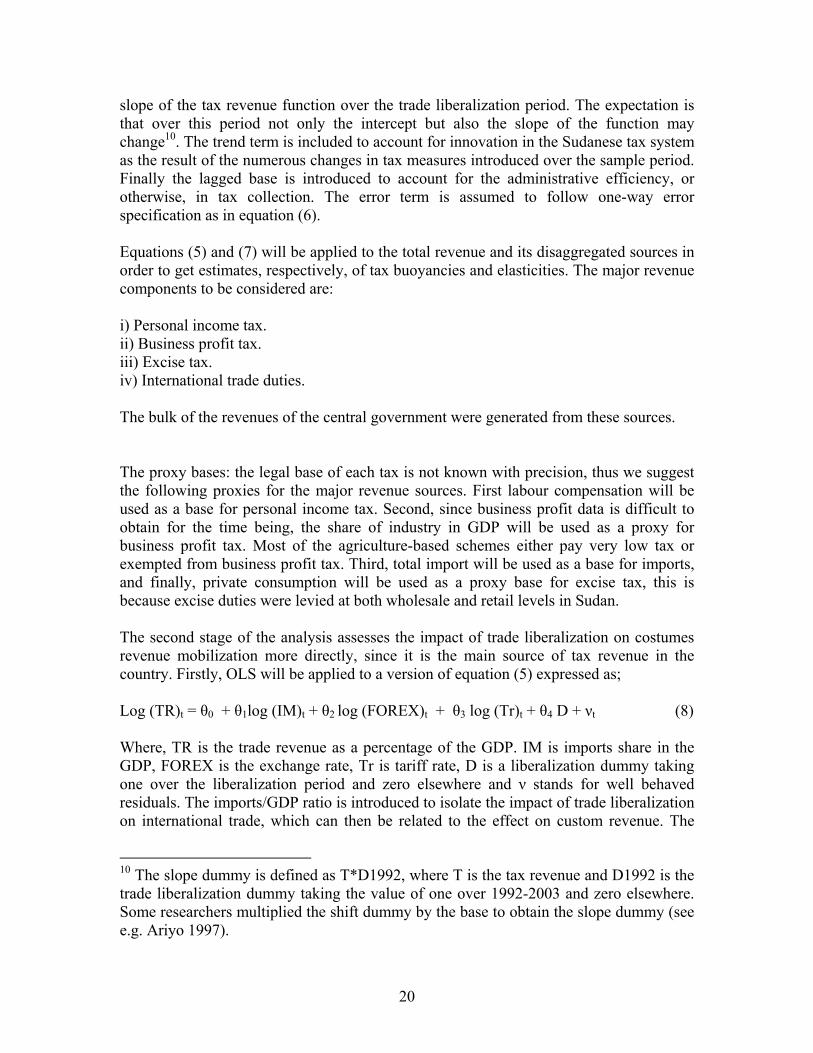
slope of the tax revenue function over the trade liberalization period. The expectation is that over this period not only the intercept but also the slope of the function may change10. The trend term is included to account for innovation in the Sudanese tax system as the result of the numerous changes in tax measures introduced over the sample period. Finally the lagged base is introduced to account for the administrative efficiency, or otherwise, in tax collection. The error term is assumed to follow one-way error specification as in equation (6). Equations (5) and (7) will be applied to the total revenue and its disaggregated sources in order to get estimates, respectively, of tax buoyancies and elasticities. The major revenue components to be considered are: i) Personal income tax. ii) Business profit tax. iii) Excise tax. iv) International trade duties. The bulk of the revenues of the central government were generated from these sources. The proxy bases: the legal base of each tax is not known with precision, thus we suggest the following proxies for the major revenue sources. First labour compensation will be used as a base for personal income tax. Second, since business profit data is difficult to obtain for the time being, the share of industry in GDP will be used as a proxy for business profit tax. Most of the agriculture-based schemes either pay very low tax or exempted from business profit tax. Third, total import will be used as a base for imports, and finally, private consumption will be used as a proxy base for excise tax, this is because excise duties were levied at both wholesale and retail levels in Sudan. The second stage of the analysis assesses the impact of trade liberalization on costumes revenue mobilization more directly, since it is the main source of tax revenue in the country. Firstly, OLS will be applied to a version of equation (5) expressed as; Log (TR)t = θ0 + θ1log (IM)t + θ2 log (FOREX)t + θ3 log (Tr)t + θ4 D + νt (8) Where, TR is the trade revenue as a percentage of the GDP. IM is imports share in the GDP, FOREX is the exchange rate, Tr is tariff rate, D is a liberalization dummy taking one over the liberalization period and zero elsewhere and ν stands for well behaved residuals. The imports/GDP ratio is introduced to isolate the impact of trade liberalization on international trade, which can then be related to the effect on custom revenue. The

10 The slope dummy is defined as T*D1992, where T is the tax revenue and D1992 is the trade liberalization dummy taking the value of one over 1992-2003 and zero elsewhere. Some researchers multiplied the shift dummy by the base to obtain the slope dummy (see e.g. Ariyo 1997).

21

exchange rate is included to capture the macroeconomic effects of this policy. The average tariff rate and the trade liberalization dummy account for the effects of trade liberalization. Secondly, we evaluate the impact of trade liberalization on the capture of evaded taxes. It is often hypothesized that lower duties-- due to trade liberalization for example-- can encourage compliance by reducing the “benefits” of the underground activities such as tax evasion, avoidance and rent-seeking, and hence improve revenue mobilization. Although there is no direct theory-based test of this hypothesis, the research utilizes two indirect techniques often discussed in the monetary approach on the issue. These are Tanzi and Guttman techniques. Tanzi (1983) assumed that the underground activities are more cash intensive than the official economy; an increase in tax is expected to increase demand for currency11. Hence he used the following currency demand function with and without tax for the estimation of the size of the undergoing economy; C = F(Y-T, R) (9) Where C is currency, (Y-T) is the after tax income, R is the rate of return on money. Equation (9) will be adapted for the case of Sudan in the following way: the inflation rate is included as a proxy for the cost of holding currency given the high rate of inflation and the constancy of the bank rate of return on money in the country. The free exchange rate premium will also be included. The expectation is that an increase in the premium signals deprecation of the exchange, which in turn might induce cash holding by agents to smooth exchange fluctuations. It may also reduce cash holding through the currency substitution motive. The sign of coefficient on this variable is an empirical issue. The ratio of labour compensation to the national income will be included. This ratio is expected to correlate positively with currency holding. The ratio of the expenditure on social services to the national income is included in order to capture the incentive on the part of agents to hide currency. Accordingly equation (9) can be expressed in log as; Log c/m2= a0 + a1log (y) + a2log (w/y) + a3log (pre) + a4log (π) +a5log (e/y) + ∑i

iiTa6 + Di + ε (9’)

Where c/m2 is the ratio of currency to broad money, (w/y) is the ratio of wages and salaries to GDP, (pre) is the premium, defined as the log of free exchange rate to the official exchange rate, (π) is the rate of inflation, (e/y) is the ratio of expenditure on social services to the GDP, Ti are the major tax rates D is a dummy variable included to capture the effect of the decline in tax revenues in the early 1980s and ε is a stochastic term. The difference between the with and without tax estimates of equation (9’) gives a measure of the nominal currency holding in the underground economy at time (t). 11 Underground activities refer here to the legal, informal and illegal dealings including cash transactions effected with the intention of avoiding tax collectors.

22

Assuming constant velocity, the share of underground economy in GDP can be determined, and then the amount of evaded tax is calculated. Hence the extent of the captured revenue, as a result of the liberalization reform, can be evaluated using the underground’s economy GDP as tax base. Guttman approach will also be applied for the same purpose. The formula often used to estimate the size of the underground activities following Guttman (1977) is expressed as;

)]/1(1[)rC/DDDD(1

FORECNUNGACT rDDCDDM +−+

= (10)

where, UNGACT refers to the nominal GDP associated with the underground activities, FORECN is the formal GDP, C/DD is the ratio of currency to demand deposit, M1 is the narrow money --currency in circulation plus demand deposit-- and the subscript r denotes the reference year. The maintain assumption in this approach is that the reference year is characterized by a normal C/DD ratio which will prevail in the economy had it not been for the growth of the underground activities. The main criticism of this approach is that the choice of the reference year may be subjective. However in the application in this study the choice of the reference year will be data based. The third stage of analysis looks at the stability role of the main fiscal variables in Sudan. As noted, an important property of the tax system is that, both revenue and expenditure growth should be smoothed through the business cycle in order to lessen the effects of macroeconomic fluctuations. We use the non-agricultural GDP12 in order to shed light on the stability role of the fiscal variables in Sudan. The degree of co-movement of series yt with output variable xt can be measured by the correlation coefficient p(j), j ε (0,±1, ±2,..). These correlations are between the stationary parts of both series to be obtained using the same filter. Series yt is deemed to be procyclical, acyclical or countercyclical depending on the whether the contemporaneous correlation coefficient p(0) is positive, zero or negative. The cross-correlation coefficient p(j), j ε (0,±1, ±2,..) indicates yt leads the cycle by j period(s) if |p(j)| is maximum for a positive j, lags the cycle if |p(j)| is maximum for a negative j and synchronous if |p(j)| is maximum for j=0. (See Agenor et al 1999). V. Estimation Results and Discussion Buoyancy The nominal measure of buoyancy of the whole tax system and of its major components were obtained by the estimated regression coefficients and were presented in table (6)13. 12 The behaviour of the agricultural output is influenced by weather conditions more than by business cycle variables. 13 These estimates were obtained using equation (5). Cochrane-Orcutt Method was used whenever Durbin Watson statistic detects serial autocorrelation of the error term (see appendix B).

23

As seen the buoyancy of the total tax revenue was estimated at 0.92, which was marginally below unity. Taxes on personal income and business profit were generally buoyant. These results compare with those obtained for other similar countries (see e. g. Osoro 1993, Muriiti 2003 and Chipeta 2002). The estimated coefficient of import duties implies that this tax is not buoyant. The low buoyancy on international trade might be due Table(6): Estimates of Tax Buoyancy in Sudan 1970-2002/1 Independent variable Equation Constant Coefficient R2 S.E. DW F (p-value) Total Tax Revenue -1.33 0.92 0.99 0.21 1.90 (0.00) (5.5) (46.1) Personal Income Tax -4.67 0.95 0.99 0.37 1.65 (0.00) (-7.71) (19.5) Business Profit Tax -3.88 0.96 0.99 0.41 1.83 (0.00) (6.1) (18.7) Import Duties -1.7 0.87 0.99 0.20 2.00 (0.00) (-12.9) (77.6) Excise Tax -3.69 0.96 0.99 0.23 1.91 (0.00) (-4.8) (17.6) Indirect Tax -1.49 0.91 0.99 0.16 1.93 (0.00) (-8.4) (61.9) Direct Tax -3.21 0.95 0.99 0.40 1.75 (0.00) (-5.6) (19.1) 1/. S.E. is the standard errors of the regression, DW is Durban-Watson statistic and the t-values were reported in brackets. All the equations have good fit as indicated by the high R2 and the significant probability value of F-statistic. The t-statistics indicate that the slope coefficients are all significant. (See appendix B). to tax evasion, tax exemptions, corruption in tax administration and the presence of the underground economy. Estimates of real measures of revenue productivity over the review period considerably diverge from their nominal estimates suggesting that inflation significantly eroded tax revenue in the country. The overall buoyancy was estimated as 0.25, however the coefficient was not precisely estimated, it compares with bouncy estimates for a group of selected low-income countries reported in Jha 2005 and Teera 200214. The only statistically significant coefficient was estimated for the excise tax, but it was 14 point lower than its corresponding nominal measure (see table 11 and appendix B1). In order to compare the performance of the tax system before and after liberalization, nominal estimates of the intercept and the coefficients for different taxes over 1970-91 and 1992-2002 were reported in tables (7) below. As seen the overall buoyancy showed a decline of 12% after the reform. The table reveals that the estimated values of both the coefficients and constants of the overall tax and the major tax handles move in the 14 We note that he dependent variable in the buoyancy equation in these studies was ratio of tax revenue to the GDP and a trend term is also included.

24

opposite direction for all these taxes. In addition, not all estimated constants were significant, making it difficult to give firm comment on the changes of buoyancies. However, it seems that the highest decline was in the case of business profit tax followed by personal income tax. Import tax is a major source of tax revenue in the country, it contributes by 40.8% to total tax revenue over the review period. It is the only tax source that showed a positive increase in buoyancy over the reform period, despite the decline in its share in total tax from 47.3% before the reform to 28% over the reform period. The decomposed buoyancies can be used to investigate the sources of loopholes in revenue leakages. Table (8) presents a summary of decomposed nominal measures of buoyancies of the major tax sources. As seen in the table the highest growth of base-to-income occurs in the case of business profit tax indicating a high growth of taxable business profit. However, business profit tax collections, measured by tax-to-base elasticity, declined by 46% over the reform period suggesting that there is an urgent need to improve the administration of collection of this tax. Table (7): Comparison of Tax buoyancies over 1970-91 and 1992-2002/1 Independent variable Independent variable Difference 1980-1991 1992-2002 Equation Constant Coefficient Constant Coefficient in Coefficients Total Tax Revenue -1.08 0.88 1.22 0.76 -0.12 Personal Income Tax -4.92 0.97 -0.24 0.67 -0.30 Business Profit Tax -4.01 0.96 -2.70 0.56 -0.40 Import Duties -2.21 0.93 -3.02 0.94 +0.01 Excise Tax -3.40 0.92 -1.68 0.84 -0.08 1/. See appendix C1. The relatively slow growth of taxable personal income of only .06% over the reform period reflects the low growth of labour share in GDP and the slow adjustment of nominal wages to inflation. The base-to-income elasticity of imports declined by 14% over the reform period implying a slow growth of dutiable imports, however, import tax were elastic with respect to base over the reform period probably reflecting improvement in the administration of this tax. Excise tax showed a decline of both base-to-income and tax-to-base elasticities over the reform period, which is a reflection of a low growth of private consumption, the proxy base of this tax, and the slacks in collection of the tax.

25

Table (8): The decomposed Tax Buoyancies Over the Reform and Pre-Reform Peroids/1 Period 1970-1991 1992-2002 Difference Base-to-Income Elasticity Personal Income Tax 0.80 0.86 +0.06 Business Profit Tax 0.92 1.40 +0.48 Import Duties 1.00 0.86 -0.14 Excise Tax 0.98 0.74 -0.24 B: Tax-to- Base Elasticity Personal Income Tax 0.64 0.44 -0.20 Business Profit Tax 1.05 0.59 -0.46 Import Duties 0.32 1.05 +0.73 Excise Tax 0.87 0.70 -0.17 1/. See appendixes C2 and C2. Overall, it appears that over the reform period the low growth of proxy bases of import and excise taxes in proportion to the GDP accounts for the decline in tax yield from these sources. While inefficiency in tax administration and slacks in collection appear to be the major causes of decline in tax effort for business profit and personal income taxes. Elasticity Nominal estimates of the elasticities of the major taxes and of total tax revenue were shown in table (9) using Singer’s (1968) type of approach15. As seen in the table the overall elasticity is 0.82, while the elasticities of individual taxes were divergent. The elasticity of import duties, the main tax in the country, was 0.83. Excise tax has an elasticity of 0.82, while both income and profit tax had respectively elasticities of 1.26 and 1.57.

15 These estimates were obtained using equation (6) without dummies, lagged base and trend terms. Cochrane-Orcutt Method was used whenever Durban Watson statistic detects serial autocorrelation of the error term (see appendix E).

26

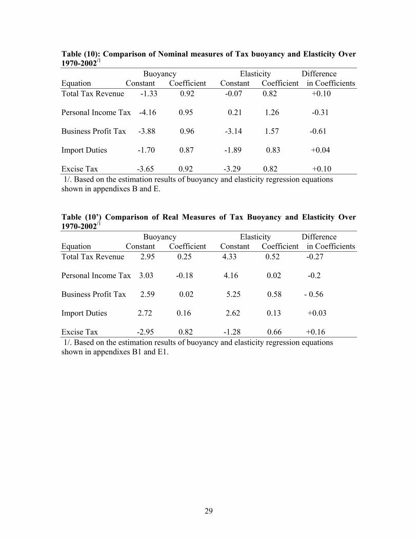
The overall tax elasticity of 0.82 implies that the growth of tax yield in proportion to the nominal growth of the economy is low. The elasticities of the income and profit taxes were greater than unity, however, the lagged base is negative implying that there were substantial administrative inefficiencies in the collection of these taxes. For a country like Sudan experiencing high inflation, lags in tax collection can be very costly to the treasury. In this context the World Bank’s CEM (1990) indicated that for the years 1976-89, if collection from business profit tax in each year were divided by the GDP of the preceding year instead of the current year the overall ratio of profit tax increases by 25%. The liberalization dummy was significant only for income tax, however the slope shift dummy was significantly positive making it difficult to assess the impact of liberalization on tax yield from this source. These two coefficients were not significant for the other tax handles indicating that liberalization has no effects on these revenue sources16. The dummy for abolition of the conventional tax over 1985-86 was significantly negative for income and profit taxes. The negative sign on this variable for these and other taxes reflects the effects of the confusion created in the tax system resulting from the replacement of the conventional tax handles with new ones. The trend coefficient was significantly negative for excise tax implying that the various reforms and innovations in the tax system failed to raise revenue from this tax source. This coefficient picked up the declining trend of the excise tax resulting from weak administration and the various tax exemptions schemes introduced to encourage local production and import-substituting industrialization. Real measures of the elasticities were all lower than their corresponding nominal estimates. The estimated coefficients of the elasticities of the overall tax and excise duties were statistically significant the others were not (see table 11 and appendix E1). This implies that inflation considerably crippled the ‘automatic’ growth of real revenues in relation to the growth of real income. Table (10) provides a summary of estimated values of the constants and coefficients for buoyancy and elasticity using nominal variables over the sample. As seen in the table, the difference between the estimated coefficients of the overall buoyancy and elasticity is positive and relatively large. However, the values of estimated constants move in different directions over the sample making it difficult to confirm that the various discretionary tax changes improve tax yield. The same observation applies to the excise duties. In contrast, for the personal income and business taxes the difference between buoyancy and elasticity were large and significant, and since the values of estimated constants move in the same direction it can be concluded that the various (DTMs) appear not to improve tax yields from these sources. In the case of import duties the values of estimated constants and coefficients move in the same direction implying that for any one percent increase in GDP the discretionary tax changes mobilize an additional 0.04 percent of revenues from import duties. Table (10’) shows a summary of the estimates of

16 This result will be further qualified in considering the import tax revenue function latter on.

27

real measures of buoyancy and elasticity. Despite the statistical insignificance of many estimated coefficients, the reported results parallel the earlier ones and confirm the ineffectiveness of the various reforms and (DTMs) in enhancing the productivity of the tax system. The significant and relatively high estimates of real measure of the excise duties indicate that the composition of total tax is skewed away from trade and income taxes towards domestic indirect tax.

28

Tab

le (9

): E

stim

ates

of T

ax E

last

icity

in S

udan

197

0-20

02/1

Equa

tion

C

onst

ant

Coe

ffic

ient

Libe

raliz

atio

n D

umm

y Sl

ope

Dum

my

Zaka

t D

umm

y 19

87-r

efor

m

Dum

my

Tren

d La

gged

B

ase

R2

DW

Tota

l Tax

Rev

enue

-.0

69

(-.0

61)

0.82

(3

.21)

1.

8 (0

.93)

-0

.09

(-0.

51)

-0.1

6 (-

0.91

) 0.

12

(0.6

3)

0.00

2 (0

.09)

0.

014

(.05)

0.

99

1.60

Pers

onal

Inco

me

Tax

0.

21

(0.2

0)

1.26

(3

.01)

-3

.89

(-3.

07)

0.61

(3

.83)

-0

.64

(-2.

58)

0.08

(0

.27)

0.

23

(4.3

1)

-1.2

2 (-

3.37

) 0.

99

1.63

Bus

ines

s Pro

fit T

ax

-3.1

4 (-

1.50

) 1.

57

(3.5

4)

4.30

(1

.13)

-0

.32

(-0.

84)

-0.5

8 (-

1.90

) 0.

03

(0.0

8)

0.04

(0

.52)

-0

.77

(-1.

82)

0.99

1.

66

Impo

rt D

utie

s -1

.89

(-2.

34)

0.83

(4

.98)

-0

.46

(-0.

48)

0.00

1 (0

.02)

-0

.11

(-1.

12)

-0.1

6 (-

1.25

) 0.

04

(1.2

5)

0.01

(0

.04)

0.

99

2.51

Exci

se T

ax

-3.2

9 (-

2.19

) 0.

82

(2.7

5)

1.03

(0

.58)

-.0

1 (-

0.1)

.0

15

(0.0

8)

0.49

(1

.98)

-0

.13

(-2.

19)

0.27

(0

.85)

0.

99

1.78

Indi

rect

Tax

-0

.44

(-0.

52)

0.67

(3

.55)

0.

21

(0.1

6)

0.03

(0

.8)

-0.2

0 (-

0.74

0.

22

(2.1

6 0.

01

(0.2

0)

0.10

(0

.47)

0.

99

1.82

Dire

ct T

ax

-1.5

6 (-

0.61

) 1.

33

(2.5

7)

1.74

(0

.38)

-.0

6 (-

0.31

) -0

.29

(-0.

87

-0.2

4 (-

0.87

) 0.

12

(1.0

4)

-.076

(-

1.45

) 0.

99

1.76

1/. S

.E. i

s th

e st

anda

rd e

rror

s of

the

regr

essi

on, D

W is

Dur

ban-

Wat

son

stat

istic

and

the

t-val

ues

wer

e re

porte

d in

bra

cket

s. A

ll th

e eq

uatio

ns h

ave

good

fit

as in

dica

ted

by th

e hi

gh R

2 and

the

sign

ifica

nt p

roba

bilit

y va

lue

of F

-sta

tistic

. The

t-st

atis

tics

indi

cate

that

the

slop

e co

effic

ient

s ar

e al

l si

gnifi

cant

. (Se

e ap

pend

ix E

)

29

Table (10): Comparison of Nominal measures of Tax buoyancy and Elasticity Over 1970-2002/1 Buoyancy Elasticity Difference Equation Constant Coefficient Constant Coefficient in Coefficients Total Tax Revenue -1.33 0.92 -0.07 0.82 +0.10 Personal Income Tax -4.16 0.95 0.21 1.26 -0.31 Business Profit Tax -3.88 0.96 -3.14 1.57 -0.61 Import Duties -1.70 0.87 -1.89 0.83 +0.04 Excise Tax -3.65 0.92 -3.29 0.82 +0.10 1/. Based on the estimation results of buoyancy and elasticity regression equations shown in appendixes B and E. Table (10’) Comparison of Real Measures of Tax Buoyancy and Elasticity Over 1970-2002/1 Buoyancy Elasticity Difference Equation Constant Coefficient Constant Coefficient in Coefficients Total Tax Revenue 2.95 0.25 4.33 0.52 -0.27 Personal Income Tax 3.03 -0.18 4.16 0.02 -0.2 Business Profit Tax 2.59 0.02 5.25 0.58 - 0.56 Import Duties 2.72 0.16 2.62 0.13 +0.03 Excise Tax -2.95 0.82 -1.28 0.66 +0.16 1/. Based on the estimation results of buoyancy and elasticity regression equations shown in appendixes B1 and E1.

30

Estimation of Tax Evasion Tax evasion is intrinsically difficult to measure, however, it is presumed that there is a strong link between tax evasion and the spread of unrecorded transactions associated with the underground economy. An indirect method of estimation was used as suggested in the methodology section to measure the size of the underground economy, having done that, the average tax rate was applied to arrive at an estimate of tax evasion as described below. Equation (9’) was estimated using annual data over 1970-2002, four tax rates relating to the major taxes in the country were included. The real per capita consumption expenditure by the private sector was included to allow for currency demand arising from increasing expenditure. The lagged currency to M2 ratio, the dependent variable, was included to capture adjustment in currency holding by agents. The ratio of social expenditure to GDP was entered to proxy the incentive of household to hide part of their activities. The demand of currency is also driven by the other motives as indicated earlier. In order to avoid the problems of ‘spurious’ regression results the Augmented Dicker- Fuller (ADF) equation was applied to test for unit root in the variables of interest. The results of the tests were shown in table (11) Table (11): ADF Unit Root Test Statistics/1 Variable level Fist Difference Lag Test-statistic lag Test-statistic C/M2 3 3.17* 2 3.67* RPPE 2 1.10 1 4.49** CPI 2 0.21 0 2.45/2

Forex 2 0.24 0 4.56* Pre 2 1.94 1 8.57** W/Y 4 0.56 4 3.02* SE/Y 1 2.97* 3 3.34* Etax 3 2.94* 3 3.21* Iduties 2 1.45 3 2.91* Itax 1 2.56/2 2 4.42** Ptax 3 2.82/2 4 4.69** Notes: 1/ADF is augmented Dickey Fuller test. The null is that the series tested contain unit root. Each variable is included with four lags; the selected lag order is determined by Akaike information criterion. The test includes a constant and a time trend for all variables in level. 2/ Schwartz Bayesian criterion indicates that t-statistic is 292. Asterisks * and ** denote rejection of the null hypothesis at 5% and 1% level respectively. All variables are in logarithms except (see appendix A for the definitions and sources of the variables).

31

As seen in the table all variable except the ratio of currency to M2, the ratio of social expenditure to income and the excise tax contain unit root in their levels while their respective first difference is stationary. Accordingly, the estimated equation contains both variables in levels and first differences. The estimation result is reported in part (a) of table (12). Table (12): Estimates of the Currency Ratio Equations/1 Variables Coefficient Standard

Errors T-value

Part (a)/1: Constant -.86 0.208 -4.13 ** Labour Compensation/GDP 0.011 0.04 0.79 Inflation (∆CPI) - .056 0.06 -0.88 Real per capita private expenditure 0.020 0.73 0.28 Premium -0.10 0.033 -2.92** Excise tax 2.75 1.05 2.61** ∆ Import duties 0.057 0.119 0.48 Personal incom tax 0.09 0.08 1.07 Business Profit tax 0.012 .16 0.076 Ratio of Social expenditure/GDP -0.045 0.016 -1.82* Dummy (1884-5) -0.06 0.04 -1.71* Lagged currrecy/M2 0.31 0.152 1.70* Part (b): Constant -.63 0.143 -4.40 ** Labour Compensation/GDP 0.014 0.045 0.76 Inflation (∆CPI) - .028 0.048 -0.572 Premium -0.093 0.028 -3.20** Excise tax 1.93 0.77 2.48** Dummy (1884-5) -0.05 0.04 -1.31 Lagged currrecy/M2 0.38 0.140 2.01** 1/. R2 =0.81 S.E.=. 055 DW= 1.92 Asterisks ** and * denote significance at 5% and 10% level respectively. Diagnostic tests: AR 1- 2 F( 2,18) = 0.359 [0.703] : Test for serial autocorrelation of residuals (H0: no autocorrelation) ARCH 4 F( 1, 18) = 0.093 [0.763]: Test for autocorrelation conditional heteroscedasticity (H0: no heteroscedasticity). Normality χ2 (2)= 0.166[0.920]: Test for normality of distribution of residuals (H0: normality) Hetero test: Chi^2(21)= 19.99 [0.522] RESET F( 1,19) = 0.109 [0.744] : Test for general misspecification of equation (H0: no misspecification). All variables are in logarithms except (see appendix A for the definitions and sources of the variables). The misspecification tests were reported in footnotes in the table. The existence of autocorrelation (AR), ARCH error, non-normal error, heteroscedastic error and model misspecification are rejected. The equation appears to perform reasonably well in terms of these tests. The excise tax was significant while the other tax rates were not. The sign

32

of the coefficient on the premium was negative and significant implying that an increase in the premium by one percent will result in a one percent decrease in the ratio of currency to M2. The sign of the coefficient of the ratio of per capita real private consumption expenditure was positive; this may reflect the cash nature of the Sudanese economy (see Kireyev 2001)17, however this coefficient was not statistically significant. The coefficient of the ratio of social welfare spending was negative as expected and significant. The adjustment coefficient of the lagged currency to M2 ratio was positive and significant at 10% level. The overall performance of the equation suggests that it can be taken as a benchmark model for the estimation of the underground economy in Sudan. The equation was also estimated without the excess sensitive components, the welfare and tax terms, however, the assumption of zero tax does not seem realistic. Thus excise tax was left in the equation as the most unavoidable tax in the Sudanese context. The result of the estimation of the equation with minimal tax is reported in table (12) part (b). The equation seems to perform well (diagnostic tests were not reported for this equation). The predicted level of the ratio of currency to M2 in each year was calculated by exponentially solving these equations. Given the actual value of M2 in each year, the predicted level of currency holding with tax (Cw) and without tax (Co) was obtained. The difference between Cw and Co indicates the extent to which currency holding is tax induced and hence gives an estimate of the “illegal” currency holding. The difference between M1 (base money) and the estimated “illegal” currency gives the legal currency holding. The income velocity of the legal money was obtained by dividing the legal money by the official GDP. Assuming that income velocity is the same in the official and underground economy, an estimate of the underground economy was determined by multiplying the “illegal” currency by the income velocity of the official economy. Table (13) presents the results of the calculation. As seen in the table the underground economy is sizable in Sudan, its percentage share to the official GDP averages about 31.4% over 1971-200218. These estimates--methodological differences aside-- fairly compare with the ratio of 38% of what Brown (1992) referred to as adjusted to unadjusted national income accounts in his discussion of international flows and capital fight in Sudan. Following the Guttman approach, as indicated earlier, the ratio of currency to demand deposit as specified in equation (10) was also used to arrive to an estimate of the size of the underground economy. Using column four in table (14) it is assumed that the

17 In other studies the sing of this coefficient was found negative implying growth in credit associated with private expenditure (see e.g. Bajada (2002). 18 Even higher estimates were obtained (not reported in the table) when simply imposing zero restrictions on the tax terms, while keeping the other coefficients unchanged as in Chipeta (2002).

33

currency deposit ratio of about (0.75) occurred in year 1981 would prevail had it not been for the growth of the underground economy19.

Table (13): Estimate of the Size of the Underground Economy Using Tanzi’s Approach (in Million Sudanese Pounds) /1

Year M1 Cw-Co “Illegal” Currency

The Size of Underground Economy’s GDP

Official GDP Underground Economy as % Of The Official GDP

1970 109.56 602.80 1971 115.32 18.62 115.79 637.50 18.16 1972 137.73 18.01 113.13 752.00 15.04 1973 168.45 35.97 243.44 896.80 27.15 1974 219.75 41.37 289.08 1246.20 23.20 1975 251.66 52.68 400.16 1510.80 26.49 1976 306.65 61.70 465.46 1848.10 25.19 1977 423.81 62.38 403.82 2339.60 17.26 1978 570.56 82.31 485.89 2882.60 16.86 1979 770.81 103.87 506.78 3253.90 15.57 1980 1040.58 152.12 680.06 3972.00 17.12 1981 1469.44 238.21 1132.50 4950.70 22.88 1982 1703.07 425.26 2342.93 7040.10 33.28 1983 2100.36 439.14 2505.44 9591.90 26.12 1984 2550.23 486.62 2784.45 11807.40 23.58 1985 4117.60 780.19 3659.16 15357.20 23.83 1986 5829.70 1084.49 4620.70 20218.10 22.85 1987 7764.30 1167.59 6649.31 36479.80 18.23 1988 11218.00 2621.39 14268.12 46791.10 30.49 1989 18898.90 3127.24 16370.38 82562.00 19.83 1990 26952.90 7758.89 44510.83 110110.70 40.42 1991 42832.20 11447.43 70211.30 192660.50 36.44 1992 95609.30 1961.37 8769.73 421818.00 2.08 1993 160409.60 38457.91 299096.75 948448.00 31.54 1994 247387.80 28915.42 222418.11 1680420.00 13.24 1995 416496.00 91481.59 994200.29 3532180.00 28.15 1996 772486.00 229290.00 4311813.70 10215100.00 42.21 1997 1016489.00 244480.58 5044512.90 15929308.00 31.67 1998 1308616.00 372668.43 7930050.30 19916126.00 39.82 1999 1696130.00 709720.60 17619204.00 24488851.00 71.95 2000 2518896.00 843293.73 18757229.00 29694524.00 63.17 2001 2715870.00 677083.08 11204439.00 33704955.00 33.24 2002 3522620.00 635543.55 8451711.20 38390966.00 22.01 1/ Based on the results of estimating equation (7’), see appendix A for the sources and definitions of the variables. 19 Other studies in the African context used year 1977 as the reference year, (see Osoro 1992 and Chipeta 2002).

34

Table (14): Estimate of the Size of the Underground Economy Using Guttman’s Approach (in Million Sudanese Pounds)/1.

Year Currency Demand Deposit

Currency/ Demand Deposit Ratio

Size of the Undergoing Economy’s GDP

Underground Economy as % of Official GDP

1970 66.82 42.74 1.56 279.99 46.45 1971 69.86 45.46 1.54 286.39 44.92 1972 75.22 62.51 1.20 194.59 25.88 1973 92.76 75.69 1.23 243.43 27.14 1974 118.75 101.00 1.18 302.83 24.30 1975 128.52 123.14 1.04 253.15 16.76 1976 152.81 153.84 0.99 256.47 13.88 1977 199.03 224.78 0.89 180.51 7.72 1978 279.06 291.50 0.96 340.79 11.82 1979 380.13 390.68 0.97 413.81 12.72 1980 508.15 532.43 0.95 462.94 11.65 1981 629.95 839.49 0.75 0.00 0.00 1982 820.41 882.66 0.93 720.28 10.23 1983 1024.49 1075.87 0.95 1106.13 11.53 1984 1247.00 1303.23 0.96 1392.72 11.80 1985 1930.40 2187.20 0.88 1159.86 7.55 1986 2760.20 3069.50 0.90 1719.25 8.50 1987 3624.70 4139.60 0.88 2609.83 7.15 1988 5601.40 5616.60 1.00 6600.18 14.11 1989 9240.60 9658.30 0.96 9733.65 11.79 1990 13112.60 13840.30 0.95 12394.55 11.26 1991 21662.90 21169.30 1.02 30040.28 15.59 1992 45316.50 50292.80 0.90 36307.65 8.61 1993 94539.70 65869.90 1.44 371090.46 39.13 1994 147902.00 99485.80 1.49 706842.63 42.06 1995 248631.00 167865.00 1.48 1474602.00 41.75 1996 444400.00 328086.00 1.35 3525658.80 34.51 1997 584944.00 431545.00 1.36 5506441.80 34.57 1998 821398.00 487218.00 1.69 10644268.00 53.45 1999 1081108.00 615022.00 1.76 14094689.00 57.56 2000 1420820.00 1098076.00 1.29 9220686.30 31.05 2001 1538360.00 1177510.00 1.31 10707349.00 31.77 2002 1935820.00 1586800.00 1.22 10298815.00 26.83 1/. Based on the results of estimating equation (8). See appendix A for the sources and definitions of the variable.

35

Table (14) presents the estimates of the absolute size of the underground economy and as a percentage of the official GDP. As seen in tables (13) and (14) the Tanzi and Guttman approaches do not give the same estimates. The latter method, compared to the former gave higher estimates in 9 years out of the 32 years considered. It also appears that Tanzi approach gave monotonically increasing estimate of the size of the underground economy except over a few years. Late in the sample both approaches appear to give comparable estimates. As noted earlier, both approaches measure the size of the underground economy as it relates strictly to the use of currency. Other forms of exchange as well as underreporting are not detected by these methods. More important, the Guttman approach imposes the assumption that there was a golden age in the past when there was no underground economy. In view of this shortcoming, the Tanzi method will be used in the estimation of the extent of tax evasion in Sudan. Table (15) gives the estimates of tax evasion in absolute terms and as a percentage of actual and potential tax revenue. Tax evasion was determined by multiplying the GDP of the underground economy by the average tax rate in the official economy20. As seen in the table, tax evasion is substantial and growing over time due to the growth of underground economy and the relatively high average tax rate in the country. Average tax evasion stands at about 53% of actual tax yield and 33% of the potential tax yield inclusive of the underground economy’s GDP. It should be noted that the estimation of the level of tax evasion reported in table (15) depends on the assumption that, the structures of the official and the underground economy are similar; but if incomes earned in the underground economy are marginal, accruing mostly to moonlighters, or relate to corruption of the tax administration, cheating in reporting, and so forth, the size of the tax evasion will be higher. The two versions of the currency approach used in the estimation underestimate the activities that are outside the cash economy; hence in all these cases both approaches give biased estimates. An important result is that, despite the liberalization reform and the reduction of the average tax rates in the economy the underground economy is sizable. Revenue loss through tax evasion is substantial and growing over time. This implies that tax reform through rate reduction alone may not be enough to check the growth of the underground economy. Such efforts should be part of a policy reform that aims at removing the remaining controls and barriers to entry into the formal economy, including the reform of the tax administration system and the simplification of its complexities. Further evidence on the effect of removing controls, through liberalization, can be obtained by the use of equation (8). As noted the equation describes the determinants of trade revenue, which is proxied by import duties. The OLS was applied to the equation in rate of growth of variables. However, the equation failed the serial autocorrelation test.

20 This rate is obtained by averaging the income tax, profit tax, excise tax and import duties.

36

Table (15): Estimates of Tax Evasion (in Millions Sudanese Pounds) Year Total tax

Revenue Potential Tax Revenue

Evaded Tax Revenue

Evaded Tax Revenue as % of Total tax Revenue

Evaded Tax Revenue as % of Potential Tax Revenue

1970 102.00 1971 110.10 134.69 24.59 22.33 18.25 1972 118.80 137.94 19.14 16.11 13.87 1973 142.80 191.74 48.94 34.27 25.52 1974 216.50 260.60 44.10 20.37 16.92 1975 245.60 321.08 75.48 30.73 23.51 1976 279.00 374.83 95.83 34.35 25.57 1977 279.50 361.49 81.99 29.34 22.68 1978 307.70 421.79 114.09 37.08 27.05 1979 337.10 432.66 95.56 28.35 22.09 1980 435.20 548.01 112.81 25.92 20.59 1981 519.40 699.63 180.23 34.70 25.76 1982 1513.60 2575.87 1062.27 70.18 41.24 1983 1244.40 2212.49 968.09 77.80 43.76 1984 1285.10 2345.56 1060.46 82.52 45.21 1985 1574.20 2615.14 1040.94 66.13 39.80 1986 1764.70 2726.30 961.60 54.49 35.27 1987 2950.00 4522.93 1572.93 53.32 34.78 1988 4707.00 7697.63 2990.63 63.54 38.85 1989 6684.80 12036.00 5351.20 80.05 44.46 1990 9572.40 20682.80 11110.40 116.07 53.72 1991 21233.50 32378.36 11144.86 52.49 34.42 1992 63632.60 65642.18 2009.58 3.16 3.06 1993 102973.00 185186.75 82213.75 79.84 44.40 1994 208670.00 324468.48 115798.48 55.49 35.69 1995 406626.50 632457.54 225831.04 55.54 35.71 1996 604587.00 1129168.40 524581.42 86.77 46.46 1997 825670.00 1394032.50 568362.46 68.84 40.77 1998 1163000.00 1805768.90 642768.86 55.27 35.60 1999 1540000.00 3072592.70 1532592.70 99.52 49.88 2000 1602000.00 3037648.50 1435648.50 89.62 47.26 2001 1879000.00 2577847.80 698847.79 37.19 27.11 2002 2137000.00 2685322.00 548322.04 25.66 20.42

37

The Cochrane-Orcutt method was used for correction for the errors. The result of the estimation is; Log (TR)t = -0.22 + 0.79*In(Import/GDP) + 2.85*In(1+Tariff) – 0.05* In(Forex) (-1.77) (12.11) (12.52) (-1.65) + 0.69*(Dslope) 0.031*(Dlib) (11.02) (1.90)

2R = 0.94 S.E.= 0.066 DW= 2.89 F (6, 24), p-value= (0.00) All variables were defined earlier and t-values are reported in parentheses. The estimated equation is of good fit, the adjusted R- squared indicates that most of the variations of the ratio of import duties to the GDP, the dependent variable, is explained by the estimated equation. All the estimated coefficients have the expected signs, the coefficient of the import/GDP ratio, the revenue case, was positive and significant at 1% level. One percent growth in this ratio leads to about 0.8% growth in the customs duties to GDP ratio. This implies an increase in the volume and value of imports relative to GDP, as a result of liberalization, raising trade tax revenue. The coefficient of the free exchange rate suggests that depreciation of the Sudanese pound relative to USA dollar leads to a fall in volume and value of imports and hence reduces trade tax revenue. However, the coefficient was not statistically significant, indicating that the value of imports in Sudanese pounds can increase compensating for the loss in revenue resulting from low trade. Overall the higher imports to GDP ratio appears to compensate for the reduction in trade revenue arising from the exchange rate effect. The coefficient of the average tariff rate is positive and significant implying that a reduction in tariff results in a significant loss of custom revenue, however, the positive coefficient of imports/GDP ratio may partly compensate for such losses. The trade liberalization dummy (Dlib) and the slope dummy (Dslope) were significant indicating that both the intercept and the slope of the import revenue function shift upwards as a result of trade liberalization. This could be taken as evidence that trade liberalization had led to an increase in trade revenue, which qualifies the result reported earlier. As we saw table (5) indicates that the base of this tax source, the ratio of imports to GDP, is high and relatively stable. The positive and statistically significant coefficient of the liberalization dummy implies that the share of the commodities subject to tariff in total imports had increased. However this cannot be taken as evidence on the positive impact of the removal of trade controls in reducing the marginal benefit of trade tax evasion. As indicated high tariff is a main determinant of customs revenue providing incentive for evasion, and that the undergoing economy is sizable and growing over the liberalization period. This section concludes by discussing the overall stabilization role of the fiscal performance over the review period. The standard macroeconomic theory suggests that the fiscal variables should be smoothed through the business cycle in order to lessen the cost of macroeconomic fluctuations. This role can be enhanced through the work of

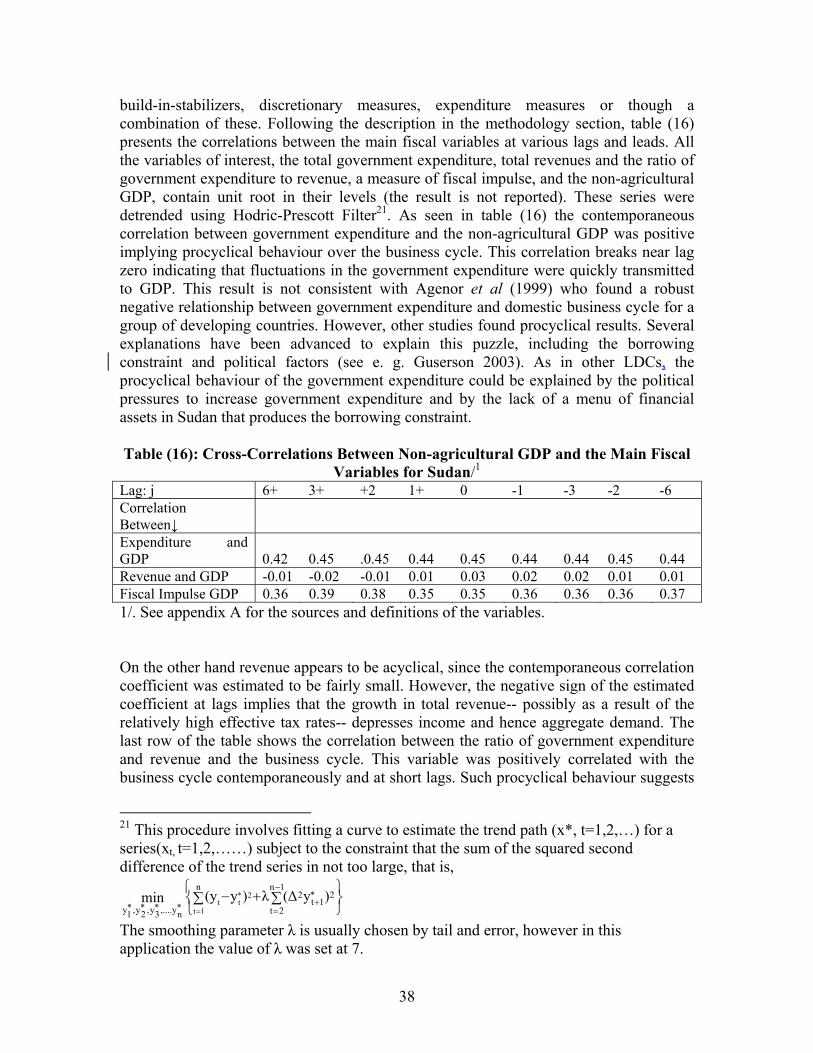
38

build-in-stabilizers, discretionary measures, expenditure measures or though a combination of these. Following the description in the methodology section, table (16) presents the correlations between the main fiscal variables at various lags and leads. All the variables of interest, the total government expenditure, total revenues and the ratio of government expenditure to revenue, a measure of fiscal impulse, and the non-agricultural GDP, contain unit root in their levels (the result is not reported). These series were detrended using Hodric-Prescott Filter21. As seen in table (16) the contemporaneous correlation between government expenditure and the non-agricultural GDP was positive implying procyclical behaviour over the business cycle. This correlation breaks near lag zero indicating that fluctuations in the government expenditure were quickly transmitted to GDP. This result is not consistent with Agenor et al (1999) who found a robust negative relationship between government expenditure and domestic business cycle for a group of developing countries. However, other studies found procyclical results. Several explanations have been advanced to explain this puzzle, including the borrowing constraint and political factors (see e. g. Guserson 2003). As in other LDCs, the procyclical behaviour of the government expenditure could be explained by the political pressures to increase government expenditure and by the lack of a menu of financial assets in Sudan that produces the borrowing constraint. Table (16): Cross-Correlations Between Non-agricultural GDP and the Main Fiscal

Variables for Sudan/1 Lag: j 6+ 3+ +2 1+ 0 -1 -3 -2 -6 Correlation Between↓

Expenditure and GDP

0.42 0.45 .0.45 0.44 0.45 0.44 0.44 0.45 0.44

Revenue and GDP -0.01 -0.02 -0.01 0.01 0.03 0.02 0.02 0.01 0.01 Fiscal Impulse GDP 0.36 0.39 0.38 0.35 0.35 0.36 0.36 0.36 0.37 1/. See appendix A for the sources and definitions of the variables. On the other hand revenue appears to be acyclical, since the contemporaneous correlation coefficient was estimated to be fairly small. However, the negative sign of the estimated coefficient at lags implies that the growth in total revenue-- possibly as a result of the relatively high effective tax rates-- depresses income and hence aggregate demand. The last row of the table shows the correlation between the ratio of government expenditure and revenue and the business cycle. This variable was positively correlated with the business cycle contemporaneously and at short lags. Such procyclical behaviour suggests

21 This procedure involves fitting a curve to estimate the trend path (x*, t=1,2,…) for a series(xt, t=1,2,……) subject to the constraint that the sum of the squared second difference of the trend series in not too large, that is,

⎭⎬⎫

∑⎩⎨⎧∑ +−

−

=+

=

1n

2t

2*1t

2n

*n,....y*

3y,*2y,*

1y)y(∆λ)y(ymin

1t

2*tt

The smoothing parameter λ is usually chosen by tail and error, however in this application the value of λ was set at 7.

39

that the fiscal impulse plays a role in driving macroeconomic fluctuations in Sudan. Again these result are not in conformity with those obtained by Agenor et al (1999) who confirm countercyclical behaviour for revenue and the fiscal impulse in all most all of their sampled countries. Implications of the Results for Policy Making Over the last three decades the Sudanese tax system experienced various changes of the individual taxes and major reforms thought to improve tax revenues, ensure equity and stabilize the economy. However these efforts leave much to be desired. A highly buoyant and tax elastic tax structure is important for a developing country like Sudan. It implies that tax revenue could increase without tampering with the tax rates and hence avoids tax evasion as well as the undesired political consequences. Therefore it is important for policy-makers to know which tax handle is more income elastic and which one is not. Reliance on income elastic taxes enhances the overall elasticity of the tax system. The results of the analysis of the buoyancy and elasticity of the Sudanese tax system reveal that the overall buoyancy and tax elasticity were below unity. Comparison of the decomposed buoyancies shows that tax-to-income elasticity was low and declining over the reviewed sub-periods for import and excise duties. This implies that there is much room for generalization of these two taxes as broad based commodity taxation. In particular, the high elasticity of tax-to-base of import duties indicates that tax yield could have been higher from this source. The relatively low tax-to-base elasticities for almost all of the major tax handles in the country seems to be a direct result of tax evasion through the underground economy, poor tax administration, tax exemptions and slacks in the enforcement of law. It follows that a tax reform, which reduces tariffs and increases other taxes, will potentially involve a loss of revenue. According tax reform should emphasize administrative efficiency, accountability of officials and enforcement of tax law. However, ceteris paribas, the potential revenue losses arising from a policy of import tariffs reduction may be compensated for by the increases in revenues resulting from growth in import base as well as by capturing evaded and avoided tariffs especially those induced by the high rates. The underground economy in the country is sizable and growing over time. This means that estimates of buoyancy and elasticity-- without considering this economy’s GDP-- will be downwardly biased. Tax evasion appears as an important problem facing tax administration in the country. Therefore, policies designed to enhance the revenue mobilization ability of the Sudanese tax system should concentrate on checking the growth of the underground economy and bringing it into the tax web. The high growth of this economy over the liberalization period indicates that tax reforms through the reduction of the effective rates alone is not enough to capture the evaded taxes, hence in addition to rate reduction administrative efficiency and the simplification of tax complexities should also be enhanced. The fiscal sector does not appear to play a role in the overall macroeconomic stability of the economy. The relatively low buoyancy and elasticity of the tax system seem to

40

negatively impact the work of build-in-stabilizers and hence amplify macro fluctuations over the course of the business cycle. This impact of the budget outcome must be acknowledged and accounted for when analyzing fiscal trends. The use of cyclically adjusted fiscal indicators could improve the efficiency of decision-making in the country. Macroeconomic policies can be geared to support the prevailing macroeconomic environment in order to facilitate successful liberalization. Particularly, policy-makers can make use of the relatively depreciated exchange rate to increase exports and growth of the GDP, hence mitigating the potential negative impact on trade revenue resulting from lowering of trade tariff. VI. Conclusion This study looked at some important aspects of the Sudanese tax system paying particular attention to the liberalization reform of 1992, which was comprehensive and have a wide reaching effects. An eclectic method was in the analysis. The following results were established First, the Sudanese tax system as a whole is not buoyant or is elastic, Comparison of nominal measures of buoyancy and elasticity over the review period indicates that tax yield from import duties has improved as a result of the various tax discretionary changes. However, in the case of other major taxes firm conclusions cannot be drawn. Real measures of buoyancy and elasticity confirm this general results and indicate that the composition of total tax is skewed away from trade and income taxes towards domestic indirect tax. Second; the before and after liberalization comparison of the nominal measures of the buoyancy of the tax system and its major handles reveals that the improvement in tax yield from import duties had occurred over the liberalization period. The positive effect of the liberalization reform on customs revenue is further confirmed by the analysis of the determinants of the productivity of the tariff revenue. The comparison of the decomposed buoyancies of taxes to their respective bases (tax-to-base elasticity) and elasticities of the bases to income (base-to-income elasticity) indicates that the base to income elasticity seems to be growing for business profit personal income taxes. The elasticity of tax-to-base is low for almost all the major tax handles in the country implying that tax collection has not increased in proportion to the growth in tax bases reflecting the combined effects of tax evasion, administrative inefficacy, tax exemptions, complexity of the tax system, corruption and slacks in enforcement of law. Third; tax evasion associated with the underground economy is the major problem facing tax administration in the country. Despite the liberalization reform, the underground economy remains sizable and growing, meaning that as yet this reform was not captured the evaded tax or checked the black and parallel markets activities. Checking of such activities is also a matter of law enforcement and improved accountability of officials.

41

Fourth; it has been shown that these is ample utility for using estimates on the budget elasticities and on the impact of business cycle on expenditure and revenue in order to improve the quality and the efficiency of the decision making process in the country. This is particularly important in view of the evidence that the fiscal sector does not appear to play a role in the overall macroeconomic stability of the economy. Finally; The less buoyant and elastic tax system, provide an explanation for the low tax efforts and the relatively low and declining government spending; which in turn implies negligence of the productive sectors of the economy. There is a considerable danger that, the rise in windfalls associated with the recent boom in oil sector, may provide lack of incentive to develop alternative tax bases and/or improve the existing ones, with the obvious result of reducing public accountability, inducing destructive rent seeking activities and an efficient allocation of the resources in the economy. References Adam, C., D. L. Bevan and G. Chambas (2000): “Exchange Rate Regimes and Revenue

Performance in Sub- Saharan Africa”, University of Oxford Working Papers No. gehwps 35.

Agenor P.R., C. J. McDermorr and E. S. Prasad (1999): “Macroeconomic Fluctuations in

Developing Countries: Some Stylized Facts”, IMF Working Paper No. 35. Andersen, S. P. (1973): “Built-in Flexibility of Sensitivity of the Personal Income Tax in

Denmark” Swedish Journal of Economics vol. 75. Ariyo, A. (1997): “Productivity of the Nigerian Tax System: 1970-1990”, AERC

Research Paper No. 67. Artus, K. K. (1974): “Tax Revenue Forecasting: A Methodological Study with

Application to Turkey”, Studies in Domestic Finance no. 5. Asher, M. G. (1989): “Fiscal System and Practices in ASEAN: Trends, Impact and

Evaluation”, Singapore Institute of South East Asian Studies. Brown, R. (1992):”Migrant’s Remittances, Capital Flight and Macroeconomic Imbalance

in Sudan’s Hidden Economies”, Journal of African Economies. Vol.86 pp86-108.

42

Chipeta, C. (2002): “The Second Economy and Tax Yield in Malawi”, AERC RP NO. 113.

Choudhry, N. N. (1975): “Measuring the Elasticity of Tax Revenue: A Divisia Index

Approach”, IMF Staff Paper, vol. 36 pp 87-122. Grunberg, I (1991): “Double Jeopardy: Globalization, Liberalization and the Fiscal

Squeeze”’ World Development Vol.83. Guserson, A. (21003):”The Optimality of Procyclical Fiscal Policy When Governments

are not Credible”, The George Washington University. Ebrill, L.p. Janet Stocky and R. Gropp (1999): “Revenue Implications of Trade

Liberalization”, IMF Occasional Papers no. 180. Ehdaie, J.(1990), “An Econometric Method for Estimating the Tax Elasticity and the

Impact on Revenues of Discretionary Tax Measures”, World Bank Working Paper No. 334, February 1990.

IMF Sudan: 2003 Article IV Consultation and First Review of the 2003 Staff-Monitored

Program--Staff Report; and Public Information Notice on the Executive Board Discussion.

Jha, R (2004): “Macroeconomic Stabilization and Pro-Poor Budgetary Policy in the

Globalize Economy”, CAMA Working Paper 8/2004. Kireyev, A. (2001):”Financial Reforms in Sudan: Streamlining Bank Intermediation”,

IMF Working Paper No. 53. Mansfield, C. Y. (1972): Elasticity and Buoyancy of a Tax System: A method applied to

Paraguay”, IMF Staff Papers Vol. 19. Muriiti M. K (2003): “Tax Reforms and Revenue Mobilization in Kenya”, AERC

Research Paper no. 131. Musgrave, R. A. (1969): “Fiscal Systems”, New Haven. Yale. Nimeiri, S. (1974): “Taxation and Economic Development: A Case Study of the Sudan”,

University of Khartoum Press. Osoro. N.E. (1993): “Revenue Productivity Implications of Tax Reform in Tanzania”, AERC

Research Paper no. 20. Prest, A.R. (1962), “The Sensitivity of the Yield of Personal Income Tax in the United

Kingdom”, The Economic Journal, September 1962.

43

Singer, N. M. (1968): “The Use of Dummy Variables in Establishing the Income Elasticity of State Income Tax Revenue”, National Tax Journal vol. 61 pp 83-90.

Stotsky, J. G. and A. WoldeMariam (1997): “Tax Effort in Sub-Saharan Africa”, IMF

Working Paper No. 107. Sury, N. M. (1985): “Buoyancy and Elasticity of Union Exice Tax Revenues in India:

1950-51 to 1980-81:’ National Council of Applied Research vol. 18, 41-56 Tanzi, V. (2003): “Trade Liberalization and Trade Tax”, A note Prepared for the Meeting

of Trade and Integration Network. August 2003. Teera, J. (2002): “Tax Performance: A Comparative Study”, Department of Economics,

University of Bath, Working Paper No. 01/2002. (1983): “The Underground Economy in US: Estimates and Implications”, Banca

Nacionale Del Lavaro Quarterly Review, Vol. 35. World Bank (2003): “Sudan Stabilization and Reconstruction: Country Economic

Memorandum”. Report No. 24620-SU. (1990): “Reversing the Economic Decline: Country Economic

Memorandum”. Report No. 8414-SU Sohato, G.S. (1961): “Indian Tax Structure and Economic Development”, New York:

Asian Publishing House Sudan Interim Poverty Reduction Strategy Paper 2004-2006”, UNDP-Sudan (2004). Thirsk, W.(1991): “Lessons From Tax Reform: an overview”, World Bank, WPS 576

Washington Dc. Wile, P. (1987):”The Second Economy, its Definitional Problems”. In S. Allesandrini and

B. Dallago (eds.), The “Unofficial Economy”, BrooKfield Gower.

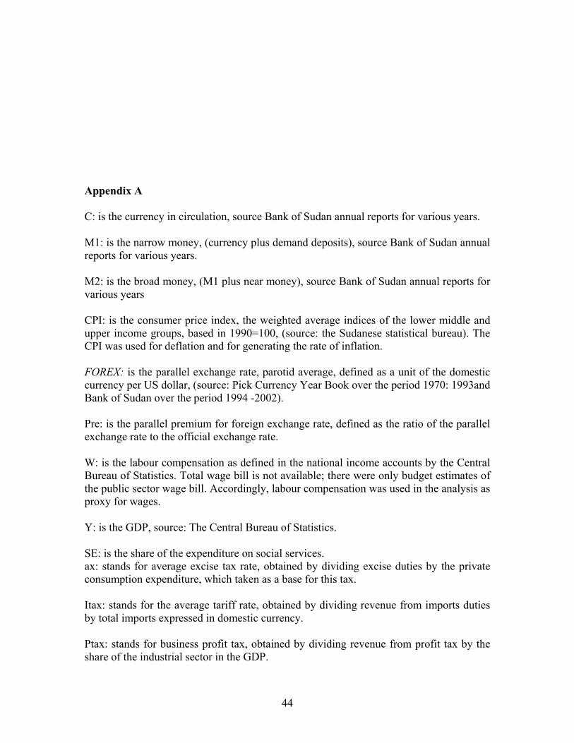
44

Appendix A C: is the currency in circulation, source Bank of Sudan annual reports for various years. M1: is the narrow money, (currency plus demand deposits), source Bank of Sudan annual reports for various years. M2: is the broad money, (M1 plus near money), source Bank of Sudan annual reports for various years CPI: is the consumer price index, the weighted average indices of the lower middle and upper income groups, based in 1990=100, (source: the Sudanese statistical bureau). The CPI was used for deflation and for generating the rate of inflation. FOREX: is the parallel exchange rate, parotid average, defined as a unit of the domestic currency per US dollar, (source: Pick Currency Year Book over the period 1970: 1993and Bank of Sudan over the period 1994 -2002). Pre: is the parallel premium for foreign exchange rate, defined as the ratio of the parallel exchange rate to the official exchange rate. W: is the labour compensation as defined in the national income accounts by the Central Bureau of Statistics. Total wage bill is not available; there were only budget estimates of the public sector wage bill. Accordingly, labour compensation was used in the analysis as proxy for wages. Y: is the GDP, source: The Central Bureau of Statistics. SE: is the share of the expenditure on social services. ax: stands for average excise tax rate, obtained by dividing excise duties by the private consumption expenditure, which taken as a base for this tax. Itax: stands for the average tariff rate, obtained by dividing revenue from imports duties by total imports expressed in domestic currency. Ptax: stands for business profit tax, obtained by dividing revenue from profit tax by the share of the industrial sector in the GDP.

45

Ptax: stands for personal income tax, obtained by dividing revenue from this source by labour compensation. (The above four proxy tax rates were generated and used due to lack of data on the actual tax rates, however these rates compare fairly well with the few available actual rates). Imports: is the total imports in domestic currency, source: the Central Bureau of Statistics. Data on the government expenditures and revenuers by type were obtained from the Ministry of Finance and National economy.

46

App

endi

x B

: Est

imat

es o

f Nom

inal

Mea

sure

s of T

ax B

uoya

ncy

in S

udan

197

0-20

02/1

In

depe

nden

t var

iabl

es

Eq

uatio

n

Con

stan

t Lo

g (G

DP)

Pa

ram

eter

s of t

he

Aut

oreg

ress

ive

Erro

r S.

E R

2 D

W

F (p

-val

ue

Tota

l Tax

Rev

enue

-1

.33

**

(-5.

49)

0.91

5**

(46.

11)

U=.

504

64*U

(-1)

+

E (

3.13

36)[

.004

]

0.21

0.

99

1.

89

(0.0

0)

Pers

onal

Inco

me

Tax

-4

.67

(7.7

1)

0.95

**

(19.

5)

U=0.64622*U(-1) +E

(4.4928)[.000]

0.

37

0.98

9 1.

65

(0.0

0)

Bus

ines

s Pro

fit T

ax

-3.8

8**

(-6.

10)

0.96

**

(18.

68)

U=0.62970*U(-1) +E

(4.1160)[.000]

0.41

0.

989

-1.8

3)

(0.0

0)

Impo

rt D

utie

s -1

.72*

* (-

12.8

9)

0.86

7**

(77.

58)

U=0.13380*U(-1) +E

(0.72613)[.473]

0.20

0.

99

2.00

(0

.00)

Exci

se T

ax

-3.6

9**

(-4.

80)

0.96

**

(17.

58)

U=0.81733*U(-1) +E

(9.0711)[.000]

0.23

0.

99

1.91

(0

.00)

Indi

rect

Tax

-1

.49*

* (-

8.41

) 0.

905*

* (6

1.9)

U=0.46533*U(-1)+E

(2.8655)[.008]

0.

16

0.99

1.

93

(0.0

0)

Dire

ct T

ax

-3.2

1**

(-5.

55)

0.94

9**

(19.

1)

U=0.60208*U(-1)+E

(3.8575)[.001]

0.40

0.

988

1.75

(0.0

0)

1/. T

he d

epen

dent

var

iabl

e is

the

Log

nom

inal

tax

reve

nue

by so

urce

. t-v

alue

s are

repo

rted

in p

aren

thes

es, o

ne st

rike

deno

tes

sign

ifica

nce

at 1

0% d

oubl

e st

rikes

den

ote

sign

ifica

nce

at 5

%.(S

ee a

ppen

dix

A fo

r the

def

initi

on o

f the

var

iabl

es)

47

App

endi

x B

1: E

stim

ates

of R

eal M

easu

res o

f Tax

Buo

yanc

y in

Sud

an 1

970-

2002

/1

Inde

pend

ent v

aria

bles

Equa

tion

C

onst

ant

Log

(GD

P)

Para

met

ers o

f the

A

utor

egre

ssiv

e Er

ror

S.E

R2

DW

F

(p-v

alue

Tota

l Tax

Rev

enue

2.

95

(1.4

2))

0.25

(0

.87)

U

=

0.69

338*

U(-

1)+E

(4

.996

6)[.0

00]

0.

21

0.41

2.08

(0

.00)

Pers

onal

Inco

me

Tax

3.03

(1.14

) -0.18

(-0.47

) U

= 0.

5508

0*U

(-1)

+E

(

3.79

10)[

.001

] 0.

30

0.34

1.53

(0

.00)

Bus

ines

s Pro

fit T

ax

2.59

(0

.95)

0.

02

(0.0

5)

U= 0.35929*U(-1)+E

(2.2116)[.035]

0.39

13

1.

86

(0.1

3)

Impo

rt D

utie

s 2.

72

(1.1

6)

0.16

(0

.49)

U= 0.82928*U(-1)+E

(7.9531)[.000]

0.24

0.

69

2.07

(0

.00)

Exci

se T

ax

-2.9

2 (-

1.33

) 0.

82**

(2

.71)

U= 0.83523*U(-1)+E

(

10.

4406

)[.0

00]

0.22

0.

70

2.06

(0

.00)

Indi

rect

Tax

2.

11

(1.2

4)

0.32

(1

.39)

U= 0.84093*U(-1)+E

( 8.

6006

)[.0

00]

0.17

0.

68

2.23

(0

.00)

Dire

ct T

ax

3.01

(1

.10)

0.

04

(0.0

9)

U= 0.41869*U(-1)+E

( 2

.648

5)[.0

13]

0.37

0.

17

1.77

(0.0

0)

1/. T

he d

epen

dent

var

iabl

e is

the

Log

real

tax

reve

nue

by so

urce

. t-v

alue

s are

repo

rted

in p

aren

thes

es, o

ne st

rike

deno

tes s

igni

fican

ce

at 1

0% d

oubl

e st

rikes

den

ote

sign

ifica

nce

at 5

%.(S

ee a

ppen

dix

A fo

r the

def

initi

on o

f the

var

iabl

es)

48

Appendix C1: Estimates of Tax buoyancies over 1970-91 and 1992-2002/1 The Pre-reform period: 1970-1991 Independent variables Equation Constant Log

(GDP) Parameters of the Autoregressive Error

S.E R2 DW F (p-value

Total Tax Revenue -1.08** (-4.93)

0.88** (35.9)

- 0.20 0.98

1.41 (0.00)

Personal Income Tax -4.92** (-7.3)

0.97** (12.9)

U=0.55909*U(-1) +E (2.8143)[.011]

0.27 0.97 2.87 (0.00)

Business Profit Tax -4.01** (-9.61)

0.96** (20.6)

U=0.62970*U(-1) +E (4.1160)[.000]

0.38 0.95 1.32 (0.00)

Import Duties -2.21** (-12.42)

0.93** (46.32)

- 0.16 0.99 2.01 (0.00)

Excise Tax -3.40 (-1.59)

0.92** (4.86)

U=0.83465*U(-1)+E (5.8188)[.000]

0.21 0.97 2.22 (0.00)

The reform period: 1992-2002 F (p-value Total Tax Revenue 1.22**

(2.70) 0.76** (26.77)

- 0.14 0.986

1.82 (0.00)

Personal Income Tax -.239 (-.129)

0.67** (5.8)

- 0.58 0.77 1.12 (0.00)

Business Profit Tax 2.70** (-5.06)

0.56** (16.75)

- 0.17 0.96 1.55 (0.00)

Import Duties -3.02** (-8.19)

0.94 (41.2)

U=-0.52852*U(-1)+E (-2.1308)[.066]

0.14 0.987 1.90 (0.00)

Excise Tax -1.68** (-2.22)

0.85** (17.9)

- 0.24 0.967 1.44 (0.00)

1/. The dependent variable is the Log tax revenue by source. t-values are reported in parentheses. (See appendix A for the definition of the variables).

49

Appendix C2/1: Estimates of decomposed buoyancy: base-to-income elasticity The pre-reform period: 1970-1991 Independent variables Equation Constant Log

(GDP) Parameters of the Autoregressive Error

S.E R2 DW F (p-value

Personal Income Tax 0.75 (-1.10)

0.80** (10.8)

U= 0.54908*U(-1)+E (2.3201)[.032]

0.29 0.96 1.68 (0.00)

Business Profit Tax -1.17** (-14.1)

0.916** (65.1)

U= 0.0041*U(-1)+E (.38362)[.706]

0.09 0.99 1.79 (0.00)

Import Duties -2.000* (-1.80)

0.995** (8.27)

U= 0.58363*U(-1)+E (2.0128)[.059]

0.31 0.96 1.50 (0.00)

Excise Tax -3.89** (-7.02)

0.976 (17.1)

U= 0.72221*U(-1)+E (3.5222)[.002]

0.11 0.99 4.74 (0.00)

The reform period: 1992-2002 F (p-value Personal Income Tax 0.21

(0.32) 0.86** (20.9)

- 0.21 0.987 1.86 (0.00)

Business Profit Tax -9.11* (1.91)

1.40** (5.06)

U= 0.59795*U(-1)+E (2.4681)[.039]

0.24 0.98 1.01 (0.00)

Import Duties -0.40 (-1.13)

0.86** (38.99)

- 0.11 0.99 2.27 (0.00)

Excise Tax 0.26 (0.05)

0.74** (2.47)

U= 0.68212*U(-1)+E ( 2.5059)[.037]

0.11 0.99 1.31 (0.00)

1/. The dependent variable is log of the given tax proxy base. t-values are reported in parentheses, one strike denotes significance at 10% double strikes denote significance at 5% . (See appendix A for the definition of the variables)

50

Appendix C3/1: Estimates of decomposed buoyancy: tax-to-base elasticity The pre-reform period: 1970-1991 Independent variables Equation Constant Log

(GDP) Parameters of the Autoregressive Error

S.E R2 DW F (p-value

Personal Income Tax 2.46 (0.16)

0.64** (2.90)

U= 0.97402*U(-1)+E (11.1117)[.000]

0.27 0.97 2.16 (0.00)

Business Profit Tax -2.21** (-6.42)

1.05** (20.47)

- 0.38 0.95 1.41 (0.00)

Import Duties 11.08 (0.39)

0.32 (1.50)

U= 0.97878*U(-1)+E (13.0248)[.000]

0.28 0.97 2.97 (0.00)

Excise Tax -2.69 (-1.53)

0.87** (5.23)

U= 0.80550*U(-1)+E (6.0381)[.000]

0.23 0.97 2.39 (0.00)

The reform period: 1992-2002 F (p-value Personal Income Tax 4.64**

(1.18) 0.44* (1.70)

U= 0.35992*U(-1)+E (1.3300)[.220]

0.45 0.70 1.98 (0.00)

Business Profit Tax 3.57** (-3.95)

0.59** (8.44)

U= 0.59795*U(-1)+E (2.4681)[.039]

0.50 0.86 0.89 (0.00)

Import Duties 3.57** (-3.95)

1.05** (20.59)

- 0.22 0.97 2.81 (0.00)

Excise Tax 0.96 (0.69)

0.695** (8.28)

U= 0.24193*U(-1)+E (0.95879)[.366]

0.13 0.97 2.13 (0.00)

1/. The dependent variable is log revenue from the given tax base. t-values are reported in parentheses, one strike denotes significance at 10% double strikes denote significance at 5% . (See appendix A for the definition of the variables)

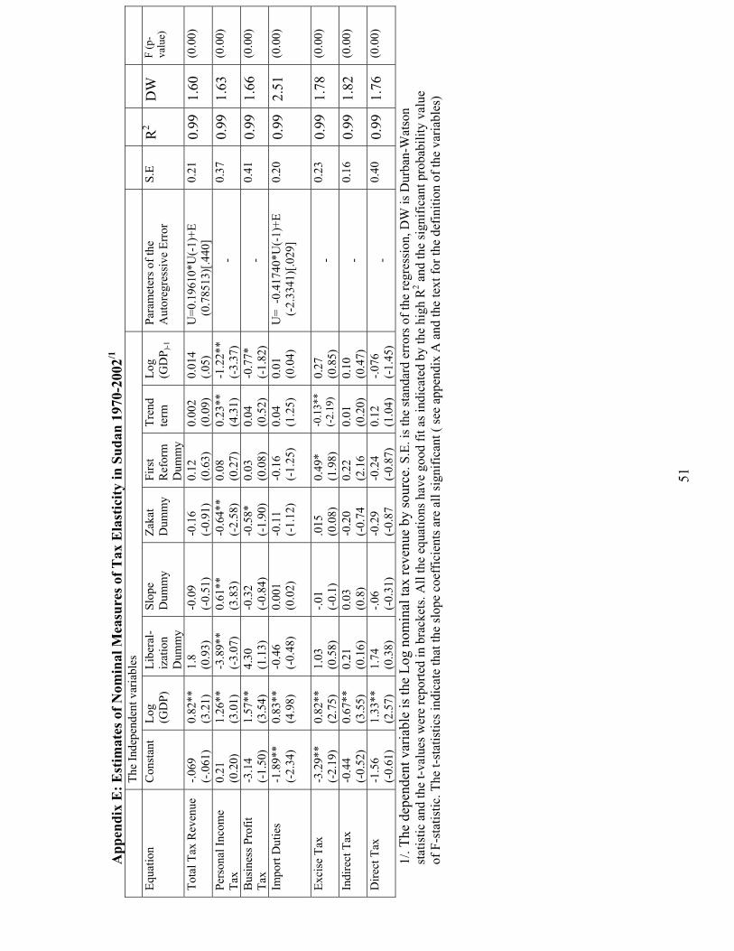
51

App

endi

x E

: Est

imat

es o

f Nom

inal

Mea

sure

s of T

ax E

last

icity

in S

udan

197

0-20

02/1

The

Inde

pend

ent v

aria

bles

Equa

tion

C

onst

ant

Log

(GD

P)

Libe

ral-

izat

ion

Dum

my

Slop

e

Dum

my

Zaka

t D

umm

y Fi

rst

Ref

orm

D

umm

y

Tren

d te

rm

Log

(GD

P )-1

Para

met

ers o

f the

A

utor

egre

ssiv

e Er

ror

S.E

R2

DW

F

(p-

valu

e)

Tota

l Tax

Rev

enue

-.0

69

(-.0

61)

0.82

**

(3.2

1)

1.8

(0.9

3)

-0.0

9 (-

0.51

) -0

.16

(-0.

91)

0.12

(0

.63)

0.

002

(0.0

9)

0.01

4 (.0

5)

U=0

.196

10*U

(-1)

+E

(0.7

8513

)[.4

40] 0.

21

0.99

1.60

(0

.00)

Pers

onal

Inco

me

Tax

0.

21

(0.2

0)

1.26

**

(3.0

1)

-3.8

9**

(-3.

07)

0.61

**

(3.8

3)

-0.6

4**

(-2.

58)

0.08

(0

.27)

0.

23**

(4

.31)

-1

.22*

* (-

3.37

) -

0.37

0.

991.

63

(0.0

0)

Bus

ines

s Pro

fit

Tax

-3

.14

(-1.

50)

1.57

**

(3.5

4)

4.30

(1

.13)

-0

.32

(-0.

84)

-0.5

8*

(-1.

90)

0.03

(0

.08)

0.

04

(0.5

2)

-0.7

7*

(-1.

82)

- 0.

41

0.99

1.66

(0

.00)

Impo

rt D

utie

s -1

.89*

* (-

2.34

) 0.

83**

(4

.98)

-0

.46

(-0.

48)

0.00

1 (0

.02)

-0

.11

(-1.

12)

-0.1

6 (-

1.25

) 0.

04

(1.2

5)

0.01

(0

.04)

U

= -0

.417

40*U

(-1)

+E

(-

2.33

41)[

.029

]

0.20

0.

992.

51

(0.0

0)

Exci

se T

ax

-3.2

9**

(-2.

19)

0.82

**

(2.7

5)

1.03

(0

.58)

-.0

1 (-

0.1)

.0

15

(0.0

8)

0.49

* (1

.98)

-0

.13*

* (-

2.19

) 0.

27

(0.8

5)

- 0.

23

0.99

1.78

(0

.00)

Indi

rect

Tax

-0

.44

(-0.

52)

0.67

**

(3.5

5)

0.21

(0

.16)

0.

03

(0.8

) -0

.20

(-0.

74

0.22

(2

.16

0.01

(0

.20)

0.

10

(0.4

7)

- 0.

16

0.99

1.82

(0

.00)

Dire

ct T

ax

-1.5

6 (-

0.61

) 1.

33**

(2

.57)

1.

74

(0.3

8)

-.06

(-0.

31)

-0.2

9 (-

0.87

-0

.24

(-0.

87)

0.12

(1

.04)

-.0

76

(-1.

45)

- 0.

40

0.99

1.76

(0

.00)

1/. T

he d

epen

dent

var

iabl

e is

the

Log

nom

inal

tax

reve

nue

by so

urce

. S.E

. is t

he st

anda

rd e

rror

s of t

he re

gres

sion

, DW

is D

urba

n-W

atso

n st

atis

tic a

nd th

e t-v

alue

s wer

e re

porte

d in

bra

cket

s. A

ll th

e eq

uatio

ns h

ave

good

fit a

s ind

icat

ed b

y th

e hi

gh R

2 and

the

sign

ifica

nt p

roba

bilit

y va

lue

of F

-sta

tistic

. The

t-st

atis

tics i

ndic

ate

that

the

slop

e co

effic

ient

s are

all

sign

ifica

nt (

see

appe

ndix

A a

nd th

e te

xt fo

r the

def

initi

on o

f the

var

iabl

es)

52

App

endi

x E

1: E

stim

ates

of R

eal M

easu

res o

f Tax

Ela

stic

ity in

Sud

an 1

970-

2002

/1

Th

e In

depe

nden

t var

iabl

es

Equa

tion

C

onst

ant

Log

(GD

P)

Libe

ral-

izat

ion

Dum

my

Slop

e

Dum

my

Zaka

t D

umm

y Fi

rst

Ref

orm

D

umm

y

Tren

d te

rm

Log

(GD

P )-1

Para

met

ers o

f the

A

utor

egre

ssiv

e Er

ror

S.E

R2

DW

F

(p-

valu

e)

Tota

l Tax

Rev

enue

4.

33**

(2

.84)

0.

52**

(2

.36)

-5

.13*

* (-

4.12

) 1.

08**

(3

.98)

-0

.32*

* (-

2.10

) -0

.22

(-1.

50)

-0.0

03

(-0.

21)

-0.4

3 (-

1.55

) -

0.

16

0.75

2.03

(0

.00)

Pers

onal

Inco

me

Tax

4.

16*

(1.9

6)

0.02

2 (0

.08)

-2

.25*

* (-

7.35

) 1.

05**

(8

.10)

-0

.67*

* (-

7.94

) -.8

5**

(-4.

37)

0.06

**

(3.3

7)

-0.4

3 (-

1.06

) -

0.21

0.

801.

74

(0.0

0)

Bus

ines

s Pro

fit

Tax

5.

25

(1.4

5)

0.58

(1

.33)

4.

30

(1.1

3)

1.11

**

(3.6

5)

-0.7

4*

(-2.

53)

-0.5

0*

(-1.

79)

0.05

**

(2.0

1)

-1.0

1*

(-1.

82)

- 0.

30

0.59

1.86

(0

.00)

Impo

rt D

utie

s 2.

62*

(1.9

9)

0.13

(0

.73)

-3

.56*

* (6

.92)

0.

86**

(5

.95)

-0

.20

(-1.

52)

-0.3

7**

(-3.

00)

0.04

11

(0.9

6)

0.07

(0

.32)

-

0.

13

0.92

1.68

(0

.00)

Exci

se T

ax

-1.2

8 (-

0.69

) 0.

66**

(2

.42)

2.

71**

(2

.68)

1.

24**

(3

.74)

.0

00

(0.0

0)

0.42

**

(2.2

7)

-0.0

9**

(-5.

75)

0.12

(0

.35)

-

0.20

0.

821.

53

(0.0

0)

Indi

rect

Tax

2.

40**

(2

.08)

0.

40**

(2

.52)

-4

.30*

* (5

.25)

1.

02**

(5

.28)

-0

.14

(-1.

17)

0.04

(0

.36)

-.0

3**

(-3.

05)

-0.0

2 (-

0.12

) -

0.11

0.

901.

99

(0.0

0)

Dire

ct T

ax

4.81

(1

.07)

07

5 (1

.46)

-4

.96*

* (-

2.99

) 1.

36**

(2

.76)

-0

.61*

(-

1.67

-0

.77*

* (-

2.08

) 0.

07*

(1.9

6)

1.05

* (1

.66)

U

=

0.13

450*

U(-

1)+E

(0.6

2006

)[.5

41]

0.34

0.

491.

92

(0.0

3)

1/. T

he d

epen

dent

var

iabl

e is

the

Log

real

tax

reve

nue

by so

urce

. S.E

. is t

he st

anda

rd e

rror

s of t

he re

gres

sion

, DW

is D

urba

n-W

atso

n st

atis

tic

and

the

t-val

ues w

ere

repo

rted

in b

rack

ets.

All

the

equa

tions

hav

e go

od fi

t as i

ndic

ated

by

the

high

R2 a

nd th

e si

gnifi

cant

pro

babi

lity

valu

e of

F-

stat

istic

. The

t-st

atis

tics i

ndic

ate

that

the

slop

e co

effic

ient

s are

all

sign

ifica

nt (

see

appe

ndix

A a

nd th

e te

xt fo

r the

def

initi

on o

f the

var

iabl

es)