The Impact of Strategic Consumer Behavior on theValue of Operational Flexibility

Gérard P. CachonThe Wharton School

University of PennsylvaniaPhiladelphia, PA 19104

cachon@wharton.upenn.edu

Robert SwinneyGraduate School of Business

Stanford UniversityStanford, CA 94305-5015swinney@stanford.edu

October 1, 2008

Chapter to Appear in Operations Management Models with Consumer-DrivenDemand, Serguei Netessine and Christopher Tang, Editors

Abstract

Increasingly sophisticated consumers have learned to anticipate future price reductions andforego purchasing products until markdowns occur. Such forward-looking or strategic behavioron the part of consumers can have a signi�cant impact on retail margins by shifting a largenumber of sales from higher, �full� prices to lower, �clearance� prices. Some �rms, however,have become adept at dealing with the strategic consumer problem by implementing variousforms of operational �exibility (for example, investing in faster supply chains capable of rapidlyresponding to changing demand conditions). A �rm famous for this strategy is the Spanishfashion retailer Zara. In this chapter, we explore the strategic consumer purchasing phenom-enon, and in particular address how the Zara model of operational �exibility impacts consumerbehavior (and, conversely, how consumer behavior impacts the value of operational �exibility).We examine in detail the consequences of volume �exibility� the ability of a �rm to adjustproduction or procurement levels to meet stochastic demand� and demonstrate that this typeof �exibility can be highly e¤ective at reducing the extent of strategic behavior. Indeed, weshow that in many cases, the value of volume �exibility is greater when consumers are strategicthan when they are not. We also show that volume �exibility is always socially optimal (i.e.,it increases the total welfare of the �rm and consumers) and may also improve consumer wel-fare (i.e., it can be a Pareto improving strategy). We also discuss the impact of other typesof operational �exibility� design �exibility, in which a product�s design can be modi�ed to suitchanging consumer tastes, and mix �exibility, in which production capacity can be dynamicallyallocated amongst several similar product variants� and argue that these types of �exibility arealso e¤ective at mitigating strategic customer purchasing behavior.

1 Introduction

Accustomed to rigid seasonality and trained by years of predictable sale patterns, consumers have

come to expect frequent and signi�cant price reductions in the retail sector. As a result, many

retailers su¤er from eroded margins generated by customers intentionally waiting for markdowns

1

Figure 1. Pricing patterns at Zara versus competing specialty retailers. Adapted from Grichnik et al.(2008).

before purchasing (Hurlbut 2004). Consumers expect deep end-of-season clearance sales, and �rms,

anxious to clear space for newer products, often oblige them. There is, however, at least one �rm

that has achieved success at managing and even preventing strategic customer purchasing behavior:

the Spanish fashion retailer Zara. There are two key components to their strategy. First, they

produce in small batches with fast replenishment lead times to their stores. Second, their initial

price for an item at the start of a selling season is not outrageously high. Consequently, they rarely

need to markdown merchandise (because they do not stock too much inventory) and when they do

o¤er a discount, it is not particularly deep (because their initial price is reasonable). These factors

combine to train Zara�s customers to avoid the �wait for the discount�strategy - if a customer sees

an item that she likes, she should purchase it now either because it will be sold at the same price

later on or it will not even be available. As a result, compared to its chief competitors, consumers

are much more likely to purchase an item at the full price at Zara (Ghemawat and Nueno 2003).

To achieve its operational �exibility, Zara produces locally (e.g., Spain, Eastern Europe or North

Africa). As a result, Zara�s leadtimes are typically less than �ve weeks for new designs and two

weeks for the replenishment of existing designs (Ghemawat and Nueno 2003). This contrasts with

their competitors who can incur average design and production leadtimes of nine months. But

Zara�s operational �exibility comes with a cost (from, for example, higher labor costs and expedited

2

shipping). Combined with Zara�s lower initial prices, one might naturally be concerned that the

company enjoys smaller gross margins per unit. However, as illustrated by Figure 1, Zara makes

up for this de�cit with volume: it typically sells a much higher percentage of its inventory at its

full price than other retailers, which can result in superior overall �nancial performance.

The goal of this article is to study the Zara model to better understand its success. We begin

with a model of consumer behavior �rst developed by Su and Zhang (2005). As in their model,

we consider a single retailer who sets an initial price and makes a production decision before the

realization of stochastic consumer demand. Each consumer decides whether to purchase at the

initial (i.e., full) price or to wait for the discount period. The discount period o¤ers a better deal

(i.e., a lower price), but there may not be any inventory left to purchase. Hence, the scarcity of

product at the discount price may make a consumer purchase at the full price.

We depart from Su and Zhang (2005) by introducing operational �exibility. With operational

�exibility the �rm can make a second production decision after observing demand, a system that is

often called quick response (see, e.g., Fisher and Raman 1996). Of course, this second production

opportunity is more expensive. However, in the absence of strategic consumer behavior, this

operational �exibility is well known to bene�t �rms by allowing them to better match their supply

to their demand. We want to assess the value of operational �exibility in the presence of strategic

consumer behavior. In particular, relative to the value of matching supply with demand, does

operational �exibility provide more or less value when consumers are strategic?

We �nd that operational �exibility is generally more valuable (but not always) when the retailer

must sell to strategic consumers. Put another way, even though operational �exibility is known

to increase pro�ts considerably with non-strategic consumers (i.e., consumers that never wait for

the discount no matter what prices are chosen) we show that it can be even more valuable when

the �rm must sell to strategic consumers, often substantially more valuable. Cachon and Swinney

(2008a) arrive at a similar conclusion, but with a signi�cantly di¤erent model. Thus, here we

provide further support for the conclusion that the presence of strategic consumers enhances the

value of operational �exibility.

The remainder of this chapter is organized as follows. In §2 we describe our approach to model-

ing production �exibility, while in §3 we discuss modeling details of strategic customer purchasing.

We then solve models of non-�exible and �exible supply chains with strategic customers in §4, and

3

discuss the incremental value of �exibility in §5. §6 presents a discussion of complications and

extensions to the basic setup, and §7 concludes the chapter with a discussion of the results.

2 Modeling Traditional and Flexible Production

We refer to our base model with non-�exible production as the traditional replenishment model. It

is also known as a newsvendor model - a canonical model in operations management that is well

suited to capture the supply-demand mismatch issues inherent in fashion retailing. This model

consists of a single �rm selling a single product with the following key features:

1. Constant Selling Price During the Season: The �rm sells the product at a constant

(�full�) price p throughout a short selling season.

2. Demand Uncertainty: The size of the market D (the number of consumers) is stochastic

and initially unknown to the �rm. The �rm has prior beliefs that the market size follows

distribution F (�).

3. Inventory Production or Procurement: Prior to learning the size of the market, the

�rm orders q units that will arrive, ready for sale, by the start of the selling season. Each

unit in this order costs c; where c < p, and so the total purchase cost is cq:

4. Supply-Demand Mismatches and End-of-Season Salvaging: The �rm sells the mini-

mum of demand D and inventory q at the full price p, and all remaining inventory is salvaged

at the markdown price s < c at the end of the season.

We assume that a large salvage market is available at the end of the season, in which the �rm

may sell all remaining units at an exogenous price s < c per unit. While such a market is commonly

assumed in newsvendor models without further justi�cation, in our model it may be useful to think

of this market as representing a second consumer segment (beyond the initial D consumers), e.g.,

a large number of �bargain hunting�customers who possess very low valuations for the product.

Cachon and Swinney (2008a) also incorporate a bargain hunting segment into their model.

This traditional replenishment model mimics the production environment of the majority of

Zara�s competitors: long design and production leadtimes lead to inventory commitment far in

4

advance of the selling season, when precise demand is still quite uncertain. As typically presented,

the newsvendor model consists of an exogenous selling price p. However, we make this price

endogenous - the �rm sets the price p at the start of the selling season (after demand information is

revealed but before any sales occur�see Figure 2). The newsvendor model with pricing is explored

by, for example, Dada and Petruzzi (1999). The nature of the pricing decision in our context is

discussed further in the next section.

In contrast to the traditional replenishment system, a �exible replenishment model represents

the system employed by Zara: greatly reduced leadtimes resulting in some inventory decisions being

made very near (or during) the selling season, when demand information is far more accurate.

Typically, the model employed to analyze this sort of production �exibility is a quick response or

reactive capacity model (see, e.g., Cachon and Terwiesch 2005). This model is identical to the

traditional replenishment model described above, with one exception: an additional procurement

opportunity is available after precise market size (D) is revealed to the �rm. As with the �rm�s

initial order, units in this second order arrive by the start of the selling season. Because this second

order is placed much closer to the start of the selling season, each unit in this second order costs

the �rm cf ; where it is natural to assume that cf > c - it is cheaper to order units in advance of

learning demand.1 (The f subscript denotes the ��exible� replenishment model.) Furthermore,

like the �rst order, there is no capacity constraint imposed on the quantity in this second order.

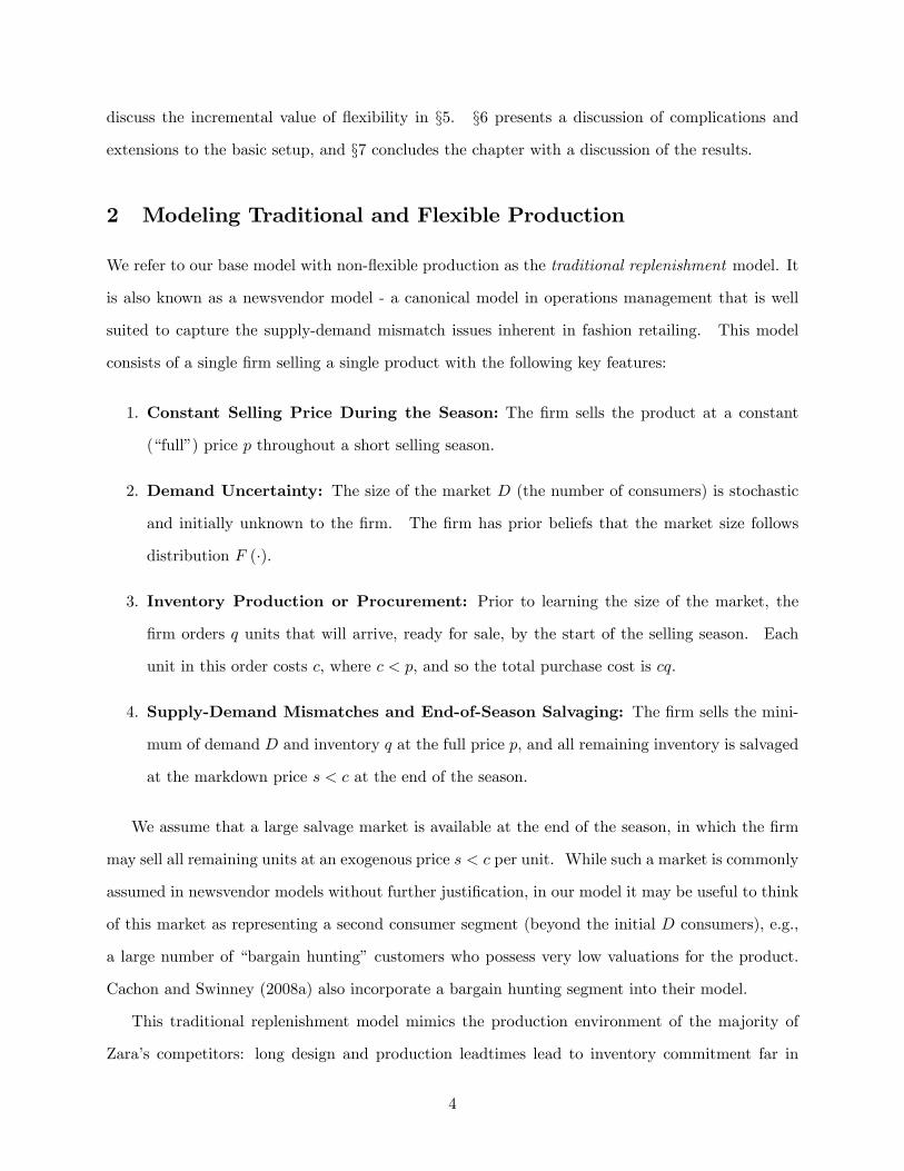
The sequence of events in the two models is presented in Figure 2.

The quick response framework frequently assumes that demand uncertainty is completely elim-

inated by the time of the second procurement�a simpli�cation, to be sure, but one that leads to

clean analytical results. In reality, the �rm may receive a series of forecast updates with each

reducing (but not entirely eradicating) error in the forecasting process. For the sake of simplicity,

we adopt the traditional assumption that uncertainty is completely resolved.2

1We describe this model as if the second order is placed before the season starts but after some demand informationis learned. In some cases, demand information is learned only at the start of the selling season and so the secondorder can only arrive at some point during the season. As long as initial season sales are highly informative, andthe lead time to receive the second order is su¢ ciently short, our model can approximately represent that situationas well - the �rst order covers sales at the start of the season and the second order should arrive before inventory isdepleted.

2We suspect that our results continue to hold even in a more complex setting with imperfect demand signals. Inparticular, even in that setting the optimal second order quantity does not depend on the full price - it is a functionof c, cf and s: Thus, our analysis would not require signi�cant modi�cation.

5

Selling Season

The firm makes aninitial procurementat marginal cost c.

The firm setsthe selling

price p.

All remaininginventory

salvaged for sper unit.

Demand uncertainty (D) is resolved.If the firm has a flexible supply

system, an additional procurementat cost cf > c is allowed.

Production/Procurement Phase

Customers arrive and makepurchasing decisions.

Figure 2. The sequence of events.

3 Modeling Strategic Consumer Purchasing

To address the issue of strategic customer purchasing behavior, we modify the classic newsvendor

and quick response settings by enriching the consumer demand model. Suppose that consumers

are risk-neutral surplus maximizers and have homogeneous valuations for the product equal to v

(constant over the entire season).3 When customers arrive at the �rm, they observe the selling

price p and whether the product is currently in-stock. We consider two types of customers: myopic

(or non-strategic) customers and forward-looking (or strategic) customers. Myopic consumers do

not consider purchasing the product at the end of the season at the markdown price, s; possibly

because they no longer value the product at the end of the season or because they do not anticipate

the price reduction. Myopic consumers have zero reservation utility and hence purchase if their

surplus is non-negative; in other words, myopic customers purchase at price p if the product is

in-stock and if

v � p � 0: (1)

Strategic customers, on the other hand, are forward-looking in the sense that they anticipate

the opportunity to purchase the product at the sale price s.4 (Implicit in this statement is the

3We model risk-neutral consumers for simplicity. Risk-averse consumers behave similarly; see Liu and van Ryzin(2008).

4A wide variety of recent models address operational issues related to such forward-looking strategic consumers,including: intertemporal pricing with no capacity constraints in Besanko and Winston (1990); pricing policies with�nite inventory in Aviv and Pazgal (2008); pricing policies for consumable goods with voluntary customer stockpilingin Su (2007); product display formats in Yin et al. (2007); and restaurant reservations in Alexandrov and Lariviere(2006); in addition to the previously cited papers.

6

assumption that consumers are capable of obtaining a unit at the salvage price�i.e., excess inventory

is cleared in a way that makes it available to the general population, as with end-of-season clearances

at fashion retailers, rather than alternative methods of salvaging such as material recycling or

industrial disposal.) Thus, these customers compare the surplus of an immediate purchase at the

full price (v � p) with the expected surplus of waiting for the sale. The value of waiting depends

on the discount price, s; as well as the chance there will be inventory remaining to purchase at the

discount price. Let � be a consumer�s expectation for the probability of being able to procure a

unit at the clearance price (more on the nature of this expectation will be discussed momentarily).

If consumers do not obtain the product at the sale price, they receive zero surplus. Expected

surplus from waiting for the sale is thus �(v� s). We assume that strategic customers purchase at

the full price if they are indi¤erent between the two options; hence, strategic customers purchase

at price p if the product is in-stock and

v � p � �(v � s): (2)

Given these assumptions, with strategic consumers there are only two candidates for equilibrium

purchasing behavior: either all consumers purchase early (at the higher price) or all purchase late

(at the salvage price).5 Because the salvage price is less than the production cost, it follows that

an equilibrium with all consumers strategically waiting results in market failure�the �rm does not

produce at all. For the remainder of the chapter, we focus on the more interesting case in which

positive production occurs, i.e., equilibria in which all strategic consumers attempt to purchase at

the full price. This implies that (2) is satis�ed in any relevant equilibrium, and � is the consumer

belief of the probability of obtaining a unit at price s conditional on all other consumers purchasing

at price p (i.e., �(v�s) is the expected surplus resulting from a unilateral deviation from equilibrium

by a single consumer).

Now we turn to the issue of how the � expectation is set. Assuming arbitrary beliefs can lead to

problems of consistency; consumers could expect � to be the probability of obtaining a unit at the

5All consumers must have the same expectation, �; value, v; and opportuntity to purchase early at the full price,p, or late at the discount price, s: Therefore either they all prefer to purchase early, v � p � �(v � s); or they allprefer to wait. Here, we assume that a consumer indi¤erent between the two options chooses to purchase early. Ifthe indi¤erent consumer chooses a mixed strategy, then the �rm could shave its full price by an in�nitesimal amountto make consumers strictly prefer purchasing early while not reducing revenue by a material amount.

7

sale price but the �rm may act in a way that leads to an entirely di¤erent probability of being able

to purchase at the markdown price. While it may not always be desirable to rule out inconsistency

on axiomatic grounds � inconsistent beliefs may be an entirely real phenomenon with important

implications �such irregularities do not appear to be the norm in the sort of predictable, seasonal

industries (such as fashion apparel) that provide our prime motivation.

It is natural, then, to seek models of customer purchasing in which beliefs are consistent with

reality: in other words, to specify that consumer expectations of �rm behavior are rational. The

idea of rational expectations �discussed in the context of �nancial markets by Muth (1961) �were

�rst formally integrated in a game theoretic framework by Stokey (1981) and Bulow (1982) to

explain the strategic consumer purchasing problem. In short, rational expectations imply that (a)

consumers have expectations of future �rm decisions, and (b) these expectations are rational and

consistent with actual �rm decisions. Such correct anticipation of �rm actions may be thought of

as the outcome of a series of repeated interactions in which consumers learn about �rm policies, for

instance, with regard to inventory availability (�my size is never in-stock at the end of the season�)

or sale pricing patterns (�this store never has deep discounts�). Our analysis in this chapter �

and a great deal of the literature on strategic consumer purchasing �makes use of the rational

expectations paradigm.

We note here that while the term rational expectations is used to highlight the fact that con-

sumers correctly anticipate �rm actions and hence behave optimally given �rm actions, this concept

is inherent in the de�nition of a Nash equilibrium with full information. For example, in a two-

player game a Nash equilibrium represents a pair of actions such that each player expects the

other player to choose the equilibrium actions and in equilibrium it is optimal for each person to

choose their equilibrium actions given their expectations. The same applies in our game - the �rm

chooses an optimal q given its belief regarding consumer actions and consumers choose optimal

actions (buy now or later) given their expectations. The subtle di¤erence has to do with what

is assumed regarding what the players know. Suppose we were to de�ne the game between the

�rm and consumers such that the �rm chooses q and consumers choose whether to purchase at

the full price or to wait for the discount. Let G(q) be the probability that inventory is available

for a consumer to purchase in the discount period conditional that all other consumers purchase

at the full price. Furthermore, assume consumers know the G(q) function. A consumer�s surplus

8

from waiting to purchase at the discount price, assuming all other consumers purchase at the full

price, is G(q)(v � s): The consumer purchases at the full price if v � p � G(q)(v � s). Note, to

evaluate an equilibrium the consumer does not need to observe the actual q choice. Instead, the

consumer infers q will be chosen because it is optimal for the �rm given the consumers�equilibrium

actions. In other words, consumers and the �rm choose their actions simultaneously. In our model

we merely replace G(q) with �; i.e., we assume consumers have an expectation for the probability

inventory is available in the discount period without necessarily knowing the mapping between the

�rm�s action, q; and that probability. To maintain consistency, we then require that in equilib-

rium G(q) = �: Therefore, the equilibrium in these two games are identical even if they make

di¤erent assumptions regarding what consumers know. Put another way, the rational expectations

terminology is technically unnecessary but we invoke this terminology for ease of exposition. (In

addition, one may argue that it makes less stringent assumptions regarding consumer knowledge

and analytical capabilities.)

Returning to our model, recall that rational expectations requires � is the actual probability

that a strategic customer successfully obtains a unit if she waits for the sale. To calculate �, we

must provide some sort of rationing rule that speci�es how inventory is allocated should demand

exceed supply at the salvage price. We employ the same rule as Su and Zhang (2005): strategic

consumers are ��rst in line�at the salvage price, followed by customers from the in�nite pool that

makes up the salvage market. This is an appealing choice for several reasons. First, customers

who arrive early in the season and intentionally choose to delay purchasing until a price reduction

may closely monitor the price of the product and �pounce� once a sale occurs. Second, if we

consider the in�nite salvage pool to be a large group of consumers with lower valuations (i.e., with

valuations equal to s), then this allocation rule maximizes consumer welfare. Third, the rule is

particularly amenable to analysis, yielding closed form equilibrium solutions to the game.6

Given this allocation rule, what is the resulting probability that a strategic consumer obtains a

unit at price s if she unilaterally deviates from an equilibrium in which all consumers purchase at

price p? Such a consumer will receive a unit at the lower price if and only if the �rm has enough

inventory (q) to satisfy all demand (D). In other words, the probability is Pr(q � D) = F (q). To6Alternative allocation mechanisms do exist and do not appear to substantially alter qualitative results: see Cachon

and Swinney (2008a) and Swinney (2008) for random rationing rules.

9

connect this result with our earlier discussion, F (q) = G(q); but as already mentioned, in a rational

expectations framework, consumers need not be aware of the actual demand distribution function,

F (q):

Having described our �rm and consumer models, we may now proceed to analyze the game

between consumers and the �rm in each of the two systems: traditional replenishment and �exible

replenishment.

4 Equilibrium analysis

This section evaluates the equilibrium choices and pro�ts for the four models constructed from

the two types of replenishment modes (traditional or �exible) and the two types of consumers

(myopic or strategic). (We do not consider models with a mixture of consumer types.) To help

keep track of notation, we use a "t" subscript to denote �traditional replenishment�(i.e., a single

order), analogous to cf ; an "f" subscript to denote ��exible replenishment� (i.e., a second order

opportunity), an "m" subscript to denote �myopic consumers� , and an "s" subscript to denote

�strategic consumers�. For example, pmf will be the �rm�s optimal full price with myopic consumer

and �exible replenishment.

4.1 Traditional Replenishment

With myopic consumers, the traditional model resembles a newsvendor model with endogenous

pricing. With strategic consumers, the traditional model mirrors the model in Su and Zhang (2005).

We replicate some of their results here to ease the comparison with the �exible replenishment model

in the next section.

We �rst observe that given the sequence of events depicted in Figure 2, and because price

is directly observed by consumers, the game is essentially one of two stages. In the �rst stage,

the �rm is a Stackelberg leader in price, and in the second stage consumers and the �rm play a

simultaneous game in inventory and purchasing. Exploiting its status as a price leader, the �rm

sets the price that yields the greatest expected pro�t; since we focus on equilibria in which all

strategic consumers purchase at the full price, this is clearly the greatest price such that either

condition (1) or (2) holds, depending on whether consumers are myopic or strategic, respectively.

10

In other words, the optimal price with myopic consumers is

pmt = v; (3)

while the optimal price with strategic customers is

pst = v � �(v � s): (4)

Note that pst � pmt; i.e., the �rm must choose a more moderate full price when selling to strategic

consumers because they will purchase early only if they enjoy a positive surplus with the full price.7

We are concerned only with equilibria in which all strategic customers purchase at the full price,

so the �rm�s expected pro�t as a function of inventory (q) and the full price (p) is

�t (q) = E�pmin (q;D)� cq + s (q �D)+

�;

where the expectation operator, E[�]; is taken over demand D, and (x)+ = max (x; 0). This

expression provides the pro�t of the �rm in both the myopic and strategic customer cases, with the

only di¤erence between the two being the optimal selling prices given by (3) and (4). For �xed p,

this function is concave in q and possesses a unique optimum. Thus, we may immediately deduce

that a �rm maximizing pro�t in the inventory-purchasing subgame invests in an inventory level q

that satis�es

1� F (q) = c� sp� s: (5)

Combining (3) with (5) yields the optimal inventory level with myopic consumers, qmt, which

satis�es

1� F (qmt) =c� sv � s: (6)

In the case of strategic consumers, we note that a Nash equilibrium with rational expectations

to the game between the �rm and strategic consumers satis�es:

7Recall, we assume that strategic consumers earn value v no matter when they make a purchase. Therefore,because the discount price, s; is lower than the full price, p; the strategic consumer strictly prefers to purchase at thediscount price if the item is available. She will purchase at the full price when she earns some surplus from doing soand there is a su¢ ciently high risk that the item will not be available in the discount period.

11

1. The �rm prices optimally, pst = v � �(v � s);

2. The �rm chooses an inventory level that maximizes expected pro�t, 1� F (qst) = c�sp�s ;

3. Consumer expectations are rational, � = F (qst) :

Combining these three conditions, we see that the unique equilibrium inventory and price satisfy

1� F (qst) =rc� sv � s and pst = s+

p(v � s) (c� s): (7)

4.2 Flexible Replenishment

In this section we address the case of �exible replenishment. Recall that the �exible replenishment

model is identical to the traditional replenishment model analyzed in the previous section, with the

following exception: after learning perfect demand information (i.e., market size D), the �rm has

the opportunity to procure additional inventory before the season begins at a higher marginal cost

cf > c. As in the previous section, q represents the quantity purchased or produced in the early

stocking opportunity.

It remains true that the optimal prices with myopic and strategic consumers satisfy (3) and (4),

respectively: acting as a Stackelberg leader in the price game, the �rm sets the greatest possible

price supported by the equilibrium. The optimal procurement at the second order point is clear:

if, after learning D, the �rm has su¢ cient inventory to cover all demand (q > D), then the �rm

orders no additional inventory. On the other hand, if the �rm has insu¢ cient inventory to cover

demand (q < D), then the �rm orders precisely enough supply to perfectly match demand (D� q)

as long as cf � p; otherwise the �rm again orders no additional inventory. Consequently, the �rm�s

expected pro�t function �with either myopic or strategic consumers �is:

�f (q) = E�pmin (q;D)� cq + s (q �D)+ + (p� cf ) (D � q)+

�:

Or, rearranging the terms of this expression,

�f (q) = E�pD � cq � cf (D � q)+ + s (q �D)+

�:

12

As in the traditional replenishment case, the pro�t function is concave in q and possesses a unique

optimal inventory quantity, given by the solution q to

1� F (q) = c� scf � s

: (8)

Note that this is independent of the full price p �consequently, the initial inventory procurement

is independent of whether consumers are strategic or myopic. This is our �rst important result

concerning the value of a �exible replenishment system. Flexibility simpli�es the �rm�s inventory

planning duties by proving to be robust to the presence of strategic customers: misjudging or

ignoring the extent of strategic customer behavior can be far less costly in a �exible replenishment

system.

From (8), we immediately deduce that with myopic customers, the optimal inventory level and

price in an �exible replenishment system satisfy

1� F (qmf ) =c� scf � s

and pmf = v, respectively. Recall that with strategic consumers, a Nash equilibrium satis�es:

1. The �rm prices optimally, psf = v � �(v � s);

2. The �rm chooses an inventory level that maximizes expected pro�t, 1� F (qsf ) = c�scf�s ;

3. Consumer expectations are rational, � = F (qsf ) :

The second condition becomes trivial in the �exible replenishment system, as the initial inven-

tory procurement is independent of the full price. Thus, combining the �rst and third conditions

yields an equilibrium full price

psf = v �cf � ccf � s

(v � s) : (9)

Again, the second term in (9) indicates that there is a �strategic consumer penalty.� If consumers

are non-strategic, the �rm merely charges v; due to forward-looking behavior, the �rm must reduce

the price to induce early purchasing.

Note that psf is decreasing in cf - as cf increases, the �rm purchases more in advance and so

the �rm needs to o¤er a lower full price to induce strategic consumers to purchase at the full price.

13

In fact, when cf = s+p(c� s) (v � s), it follows that pst = psf = cf . For any greater cf ; the �rm

�nds itself in a situation in which the second procurement opportunity is of no value because the

full price, psf ; is then less than the cost of procuring additional units. Therefore, in the strategic

consumer model the �rm uses �exible replenishments only when cf < s+p(c� s) (v � s) and does

not use �exible replenishments when

s+p(c� s) (v � s) � cf � v:

5 The Value of Flexibility

Armed with equilibrium results for both the traditional and �exible replenishment systems, we

may now address the value of �exibility � that is, the increase (or decrease) in expected pro�t

that a �rm experiences when moving from a traditional to a �exible replenishment system. When

discussing the value of �exibility, we have two choices for the unit of analysis: the absolute or the

relative value. The absolute value refers to the incremental change in �rm pro�t with either myopic

consumers, �m; or strategic consumers, �s:

�m = �mf � �mt

�s = �sf � �st

The relative value of �exibility, �; on the other hand, refers to the percentage change in �rm pro�t:

�m =�mf � �mt

�mt

�s =�sf � �st�st

Both measures can be important to a �rm exploring the value of �exibility. In this section, we

address both quantities, beginning with the relative value. Of primary interest are the following

key questions: (1) how does the value of �exibility change when consumers are strategic, rather

than myopic, and (2) what are the drivers of this change in value?

14

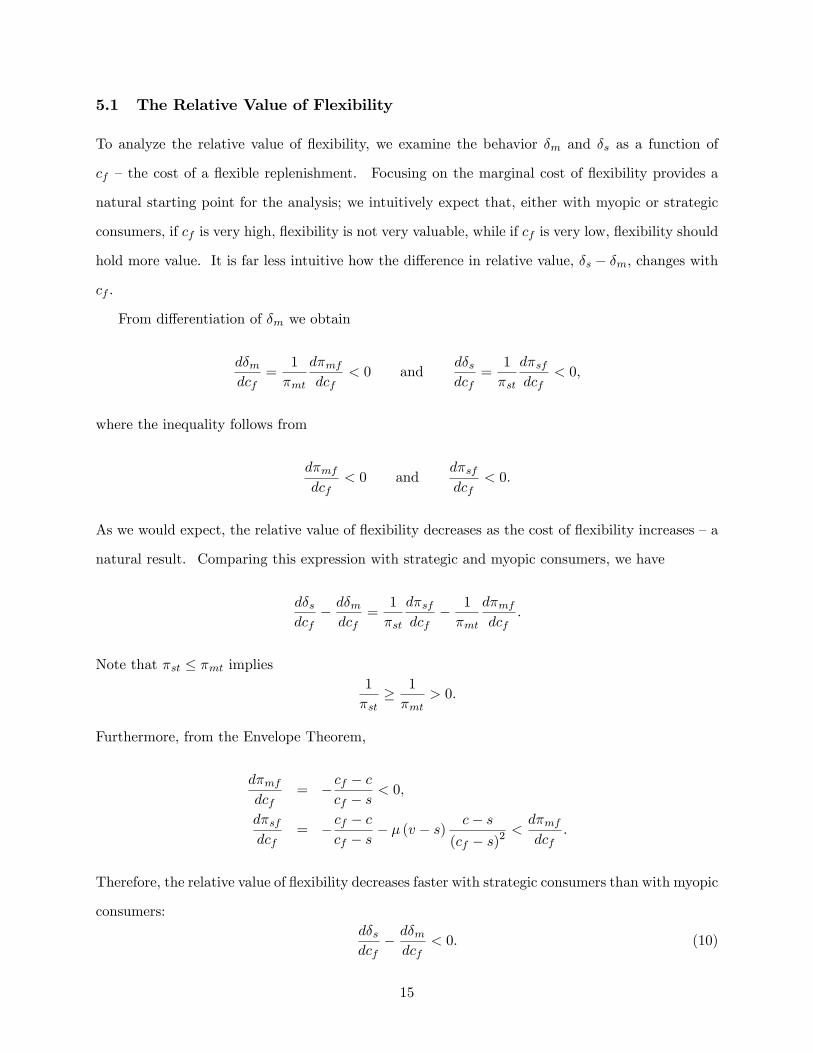
5.1 The Relative Value of Flexibility

To analyze the relative value of �exibility, we examine the behavior �m and �s as a function of

cf �the cost of a �exible replenishment. Focusing on the marginal cost of �exibility provides a

natural starting point for the analysis; we intuitively expect that, either with myopic or strategic

consumers, if cf is very high, �exibility is not very valuable, while if cf is very low, �exibility should

hold more value. It is far less intuitive how the di¤erence in relative value, �s � �m; changes with

cf :

From di¤erentiation of �m we obtain

d�mdcf

=1

�mt

d�mfdcf

< 0 andd�sdcf

=1

�st

d�sfdcf

< 0;

where the inequality follows from

d�mfdcf

< 0 andd�sfdcf

< 0:

As we would expect, the relative value of �exibility decreases as the cost of �exibility increases �a

natural result. Comparing this expression with strategic and myopic consumers, we have

d�sdcf

� d�mdcf

=1

�st

d�sfdcf

� 1

�mt

d�mfdcf

:

Note that �st � �mt implies1

�st� 1

�mt> 0:

Furthermore, from the Envelope Theorem,

d�mfdcf

= �cf � ccf � s

< 0;

d�sfdcf

= �cf � ccf � s

� � (v � s) c� s(cf � s)2

<d�mfdcf

:

Therefore, the relative value of �exibility decreases faster with strategic consumers than with myopic

consumers:d�sdcf

� d�mdcf

< 0: (10)

15

The di¤erence in the relative value of �exibility is

�s � �m =��sf�st

� 1����mf�mt

� 1�:

Now consider a particular point, cf = c; in which case �sf = �mf : Hence, for cf = c; the di¤erence

in the relative value of �exibility can be written as

�s � �m =��mf�st

� 1����mf�mt

� 1�= �mf

�1

�st� 1

�mt

�> 0:

Therefore, when cf = c; the relative value of �exibility is greater with strategic consumers than

with myopic consumers (�s > �m); but (10) indicates that �s decreases faster with cf than �mdoes.

This raises the possibility that for a large enough cf ; �s decreases to the point that it is less than �m:

In fact, this occurs. Recall that �exible replenishment provides no value with strategic consumers

when cf � s+p(c� s) (v � s): In that regime �s = 0: On the other hand, �m > 0 for all cf < v.

Consequently, there exists some cf < s+p(c� s) (v � s) such that �s > �m for all cf 2 [c; cf ) and

�s � �m for all cf 2 [cf ; v]: In words, as long as the cost of the second replenishment is not too

high (less than cf ), �exible replenishment provides greater value with strategic consumers than it

does with myopic consumers.

This result is depicted graphically in Figure 3. As the �gure demonstrates, the relative value

of �exibility with myopic consumers is rather �at, whereas the value with strategic consumers is

strongly dependent on cf . When cf is small (in the �gure, c = 3) then �exibility can o¤er an

enormous advantage with strategic consumers, resulting in a pro�t increase of over 250% in the

example.

The potentially large increase in the relative value of �exibility under strategic customer behav-

ior has signi�cant implications for how a �rm evaluates a �exible supply chain. It is well established

in the literature that �exible replenishment can provide signi�cant value when consumers are my-

opic (see, e.g., Fisher and Raman 1996, Eppen and Iyer 1997, Iyer and Bergen 1997, and Fisher

et al. 2001). Here, we �nd that �exible replenishment can provide substantially more value when

consumers are strategic as long as the marginal cost of the second replenishment is not too high,

cf < cf : However, if the marginal cost is high (cf � cf ), then �exible replenishment provides little

16

Figure 3. The relative value of �exibility as a function of the unit cost of a �exible replenishment (cf ). Inthis example, demand is normally distributed with mean 50 and standard deviation 10, and v = 10, c = 3,

and s = 1.

value in a market with strategic consumers. This occurs because strategic consumers require a

lower full price than myopic consumers to induce them to purchase at the full price. If the �exible

replenishment system cannot deliver goods at a cost lower than the full-price, it provides no value.

Referring to Figure 1, if the speciality retailer sells to myopic consumers at a price of $100, then

�exible replenishment is valuable to that retailer for any cf < $100: In contrast, Zara sells to

strategic consumers for $85, so its �exible replenishment system provides value only if cf < $85:

5.2 The Absolute Value of Flexibility

Despite the fact that we have shown that �exibility possesses greater relative value if consumers

are strategic and cf is not too high, it need not be the case that the analogous result holds with

absolute values. To see this, suppose �st = 10 and �sf = 20, yielding a relative value of 100%

and an absolute value of 10 under strategic behavior. If, for example, �mt = 100 and �mf = 150,

then with myopic customers the relative value is 50% (less than with strategic customers) while

the absolute value is 50 (more than with strategic customers). Hence, in the following subsection

we explicitly address the absolute value of �exibility.

17

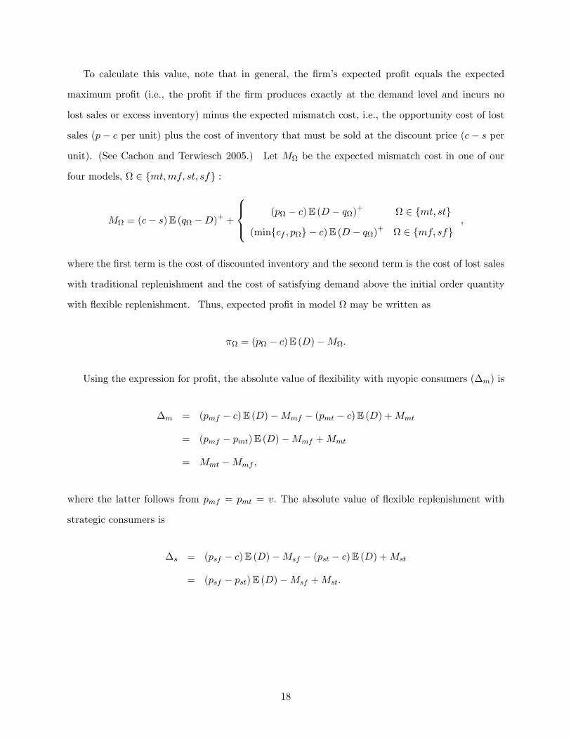
To calculate this value, note that in general, the �rm�s expected pro�t equals the expected

maximum pro�t (i.e., the pro�t if the �rm produces exactly at the demand level and incurs no

lost sales or excess inventory) minus the expected mismatch cost, i.e., the opportunity cost of lost

sales (p� c per unit) plus the cost of inventory that must be sold at the discount price (c� s per

unit). (See Cachon and Terwiesch 2005.) Let M be the expected mismatch cost in one of our

four models, 2 fmt;mf; st; sfg :

M = (c� s)E (q �D)+ +

8><>: (p � c)E (D � q)+ 2 fmt; stg

(minfcf ; pg � c)E (D � q)+ 2 fmf; sfg;

where the �rst term is the cost of discounted inventory and the second term is the cost of lost sales

with traditional replenishment and the cost of satisfying demand above the initial order quantity

with �exible replenishment. Thus, expected pro�t in model may be written as

� = (p � c)E (D)�M:

Using the expression for pro�t, the absolute value of �exibility with myopic consumers (�m) is

�m = (pmf � c)E (D)�Mmf � (pmt � c)E (D) +Mmt

= (pmf � pmt)E (D)�Mmf +Mmt

= Mmt �Mmf ;

where the latter follows from pmf = pmt = v: The absolute value of �exible replenishment with

strategic consumers is

�s = (psf � c)E (D)�Msf � (pst � c)E (D) +Mst

= (psf � pst)E (D)�Msf +Mst:

18

The di¤erence in the absolute values of �exibility can now be expressed as

�s ��m = (psf � pst)E (D)�Msf +Mst �Mmt +Mmf

= (psf � pst)E (D) +Mst �Mmt;

where the latter follows from qsf = qmf , which in turn implies Msf =Mmf : The �rst term re�ects

the use of �exible replenishment to increase its per unit revenue: psf � pst: This occurs because

�exible replenishment lowers the initial order quantity, thereby lowering the availability of inventory

in the discount period, thereby allowing the �rm to charge a higher full price (assuming psf � cf ).

The second term re�ects the di¤erences in mismatch costs with traditional replenishment.

Consider the di¤erence in the absolute value of �exibility when cf = c: In this case psf = v =

pmt; which implies

�s ��m = (pmt � pst)E (D) +Mst �Mmt

= �mt � �st > 0:

Hence, the absolute value of �exibility is greater with strategic consumers when �exibility is cheap

(when cf = c) and therefore highly e¤ective. Furthermore,

d (�s ��m)dcf

=dpsfdcf

E (D) < 0;

and so the di¤erence in absolute value of �exibility decreases as cf increases. Thus, we have

established the same pattern as with the relative value of �exibility: �s is initially greater than

�m (for cf = c) but decreases as �exibility becomes costlier. For large enough cf ; we have

established that �s = 0 (because then cf > psf ) while �m remains positive. Thus, for some value

�cf we have �s > �m for all cf < �cf and otherwise �s � �m: This pattern is illustrated in Figure

4. In this example the absolute value of �exibility can be substantially greater with strategic

consumers than with myopic consumers, upwards of 10 times more valuable.

Figures 3 and 4 also illustrate that relative and absolute values need not correspond. For exam-

ple, for the range 5 < cf < 5:25 we see that the relative value of �exibility is greater with strategic

19

Figure 4. The absolute value of �exibility as a function of the unit cost of a �exible replenishment (cf ).In this example, demand is normally distributed with mean 50 and standard deviation 10, and v = 10,

c = 3, and s = 1.

customers but the absolute value of �exibility is greater with myopic consumers. Nevertheless,

in the range cf < 5; both the relative and absolute values of �exibility are greater with strategic

consumers.

To summarize, we �nd that not only does �exibility often provide greater relative value when

consumers are strategic, it can also provide greater absolute value. This in an important result for

�rms considering implementing a �exible supply system: if their customer base is strategic, then

�exibility can provide enormous additional bene�ts over the myopic customer case, giving greater

justi�cation to spending the high �xed costs associated with implementing a �exible system.

5.3 Drivers of the Value of Flexibility

What causes the potentially large increase in the value �both relative and absolute �of �exibil-

ity under strategic customer behavior? The key lies in two distinct consequences of �exibility:

matching supply with demand, and reducing strategic behavior.

The value to the �rm of better matching supply to demand is present regardless of the type

of customer population it faces. Flexibility in our model eliminates lost sales (assuming cf � p).

Thus, the �rm uses �exibility to lower its initial purchase quantity, which reduces the cost of excess

20

inventory that needs to be marked down to the salvage price. However, the full price with strategic

consumers is lower than the full price with myopic consumers. Hence, the value of eliminating

lost sales is actually lower with strategic consumers than with myopic consumers. In other words,

the value of better matching supply with demand is higher when the full price is higher. If only

this e¤ect were present, we would conclude that �exibility is more valuable with myopic consumers

than with strategic consumers. But there is a second e¤ect.

The full price with myopic consumers is independent of whether the �rm possesses �exibility

or not, i.e., pmt = pmf = v: However, with strategic consumers, adding �exibility allows the

�rm to increase the full price, pst < psf , because �exibility reduces the initial order quantity,

qsf < qst: With less initial inventory, the �rm is less likely to sell any inventory at the salvage price

and so strategic consumers are willing to pay a higher full price. Therefore, adding operational

�exibility allows the �rm to earn a higher price on all sales. This e¤ect can dominate the former

- while �exibility helps to reduce lost sales and excess inventory, it can be more valuable to use

�exibility to increase revenue on all regular season sales. Our numerical studies indicate that not

only can this e¤ect dominate, it tends to dominate by a considerable amount over a large range

of parameters. Therefore, while we cannot conclude that operational �exibility is always more

valuable with strategic consumers, we �nd that operational �exibility is generally more valuable.

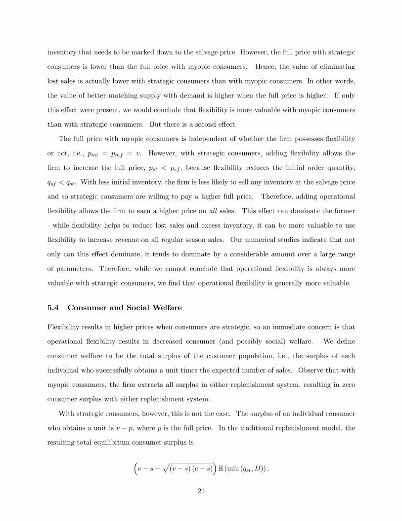
5.4 Consumer and Social Welfare

Flexibility results in higher prices when consumers are strategic, so an immediate concern is that

operational �exibility results in decreased consumer (and possibly social) welfare. We de�ne

consumer welfare to be the total surplus of the customer population, i.e., the surplus of each

individual who successfully obtains a unit times the expected number of sales. Observe that with

myopic consumers, the �rm extracts all surplus in either replenishment system, resulting in zero

consumer surplus with either replenishment system.

With strategic consumers, however, this is not the case. The surplus of an individual consumer

who obtains a unit is v � p; where p is the full price. In the traditional replenishment model, the

resulting total equilibrium consumer surplus is

�v � s�

p(v � s) (c� s)

�E (min (qst; D)) :

21

In this system, consumers pay a low price (so individual surplus is high) but not all consumers are

served. In the �exible replenishment model (again, assuming cf � psf ), total surplus is

cf � ccf � s

(v � s)E (D) :

With �exibility, consumers pay a higher price (so individual surplus is lower) but all consumers

are ultimately served. Therefore, it is not clear whether �exibility increases or decreases consumer

surplus.

Let � = E (min (qst; D)) =E (D) ; which is the �ll rate (fraction of demand that is ful�lled) with

traditional replenishment We can now write an expression for when consumer surplus is greater

with �exible replenishment than with traditional replenishment:

cf � ccf � s

� ��1�

p(c� s) = (v � s)

�:

The left hand side is increasing in cf : If we let cf equal its maximum feasible value, cf = s +p(c� s) (v � s); then the above expression can be written as

�v � s�

p(v � s) (c� s)

�� �

�v � s�

p(v � s) (c� s)

�;

which always holds (given that � < 1). Therefore, as long as cf is su¢ ciently large, �exibility

increases consumer surplus when selling to strategic consumers. This pattern is illustrated in Figure

5.

Also of interest is the impact of �exibility on social welfare, i.e., the sum of �rm and consumer

surplus. Combining consumer welfare with expected �rm pro�t, we see that social welfare in the

traditional system is

Wst = E�vmin (qst; D)� cqst + s (qst �D)+

�;

while social welfare in the �exible system is

Wsf = E�vmin (qsf ; D)� cqsf + (v � cf ) (D � qsf )+ + s (qsf �D)+

�:

22

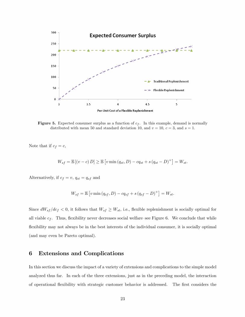
Figure 5. Expected consumer surplus as a function of cf . In this example, demand is normallydistributed with mean 50 and standard deviation 10, and v = 10, c = 3, and s = 1.

Note that if cf = c,

Wsf = E [(v � c)D] � E�vmin (qst; D)� cqst + s (qst �D)+

�=Wst:

Alternatively, if cf = v, qst = qsf and

Wsf = E�vmin (qsf ; D)� cqsf + s (qsf �D)+

�=Wst:

Since dWsf=dcf < 0, it follows that Wsf � Wst, i.e., �exible replenishment is socially optimal for

all viable cf . Thus, �exibility never decreases social welfare�see Figure 6. We conclude that while

�exibility may not always be in the best interests of the individual consumer, it is socially optimal

(and may even be Pareto optimal).

6 Extensions and Complications

In this section we discuss the impact of a variety of extensions and complications to the simple model

analyzed thus far. In each of the three extensions, just as in the preceding model, the interaction

of operational �exibility with strategic customer behavior is addressed. The �rst considers the

23

Figure 6. The value of �exibility (in terms of social welfare) as a function of cf . In this example, demandis normally distributed with mean 50 and standard deviation 10, and v = 10, c = 3, and s = 1.

impact of dynamic markdown pricing (rather than static pricing as we assume in our model) and

consumers with heterogeneous valuations. The second explores the consequences of consumers

that do not know (but learn) their valuations over time. The third discusses alternative forms of

operational �exibility, and considers their impact on strategic customer behavior.

6.1 Dynamic Sale Pricing and Consumer Heterogeneity

There are two key simpli�cations present in our the model: the end-of-season clearance price is

exogenously determined and ex ante �xed, and consumers are homogeneous both in the degree to

which they are strategic (i.e., they are either all myopic or all strategic) and in their valuation for

the good.

Suppose the �rm is allowed at the end of the season to choose to keep the full price, p; or to

lower the price to s to clear inventory in the in�nite salvage market. This does not, in the context

of homogeneous consumers, alter the analysis because all strategic consumers purchase early in

equilibrium and so the �rm always lowers the price to s at the end of the season to clear inventory.

Hence, a consumer unilaterally deviating from equilibrium �nds the product for sale at price s

during the clearance period, precisely as she would in our static pricing model.

Imagine, however, that consumers are heterogenous in their valuation for the product, pos-

24

sessing, for example, uniform valuations in a �xed interval. Because consumers are no longer

homogeneous, it need not be the case that all consumers purchase at the full price in a viable

equilibrium; indeed, it can be shown that in equilibrium, consumers with high valuations purchase

early while consumers with low valuations purchase later. If the �rm is free to set a clearance

price, the equilibrium division of consumers according to valuations will induce the �rm to price

skim�set a high price for higher value customers that purchase earlier, and set a lower price for

lower value customers who purchase later. If a large �bargain hunting�customer segment exists

(e.g., the in�nite salvage market) then the �rm may still lower the price to s if inventory during the

clearance phase is signi�cant (i.e., if demand during the full price phase is low). Thus, a dynamic

clearance price is a function of stochastic demand and the equilibrium number of consumers who

purchase at the full price. When making their purchasing decision consumers must consider all

possible future sale prices to calculate their expected surplus of waiting until the clearance sale.

What is the impact of this richer model on our results concerning supply chain �exibility?

Because �exibility lowers the amount of excess inventory, it decreases the chances that a �rm will

have to set a deep discount to clear inventory during the end-of-season sale. It also ensures that

the �rm has adequate inventory to cover demand if the product is a �hit� and prices are high.

Flexibility thus has two e¤ects: it reduces supply-demand mismatch (just as in our simple model)

and it increases the clearance price. By increasing the expected clearance price, the �rm is able to

encourage more consumers to buy at the full price; why wait for a sale if the savings are not very

signi�cant? In turn, this allows the �rm to set a higher full price and reap greater demand at the

full price. The net result is that �exibility may possess even greater value when consumers have

heterogenous valuations and sale prices are endogenously determined�in addition to the bene�ts

discussed in our preceding analysis, the �rm gains additional value from higher prices at the end

of the season.

We might also imagine other models of consumer heterogeneity, for instance heterogeneous

rates of consumption (e.g., di¤erent discount rates) or heterogeneous degrees of foresight (some

myopic consumers mixed in with strategic consumers). The intuition in such models is similar:

with dynamic pricing, �exibility helps to raise the average clearance price and thus encourage

more consumers to purchase at the full price �see Cachon and Swinney (2008a). This, in turn,

enhances the value of �exibility beyond that which we derived in our simple model. We therefore

25

conjecture that the bene�ts of �exibility in helping a �rm cope with strategic behavior are robust

to complications involving heterogeneous customer populations and various pricing schemes.

6.2 Uncertain Consumer Valuations and Learning

In the model analyzed in §§2�5, consumers are fully informed concerning their valuations at the

start of the game. While this may be true for generic goods or products with relatively simple

attributes that are easily analyzed (e.g., clothing), consumers may not initially know how much

they value some products. Examples include innovative or complex products, products with long

life cycles reliant on secondary goods of uncertain quality (e.g., video game systems), and even

experience goods. With many of these products, information about value is disseminated over

time to the customer population as, for example, expert product reviews are published, secondary

goods are released, and consumers experience the product�s features via units purchased by friends

or in-store demonstrations. See Swinney (2008) for an analysis of this problem, the key results of

which we summarize here.

With products of this type, consumers have an added bene�t to delaying a purchase: to gather

more information about the product�s value to them. In such a setting, it is possible for a �exible

supply chain to actually decrease a �rm�s pro�t (even in the absence of a �xed costs to implement

a �exible system) �by operating with an agile supply system capable of meeting future demand,

the �rm increases the overall availability of the product, thereby minimizing rationing risk and

increasing consumer incentives to learn as much information about product value as possible before

purchasing. This e¤ect can be called demand shifting �by increasing availability, the �rm causes

customers to purchase later.

When this occurs, overall demand to the �rm can actually decrease. This is because in selling

to consumers before valuations are learned � also know as advance selling, see Xie and Shugan

(2001) �the �rm inevitably induces some consumers to purchase the product who ultimately will

not value it. If customers are encouraged to delay their purchase, some of these �false positives�

are eliminated from the �rm�s demand, thereby decreasing pro�t.

There are cases, however, in which shifting demand (and subsequently reducing advance selling)

bene�ts the �rm. If, for instance, prices increase over time (e.g., due to promotional discounts

during new product introduction) or if unsatis�ed customers are allowed to return products for full

26

refunds, selling to many customers early (before value is fully learned) can actually harm the �rm;

in these cases, supply chain �exibility �which reduces the extent of advance selling �helps the

�rm by increasing the number of sales at a higher, later price or by decreasing the number of false

positive purchases resulting in costly product returns.

These results imply that �exibility can provide both positive and negative value when a �rm

sells a product for which consumers have uncertain valuations. Thus, �rms must carefully consider

the nature of their product and the ease with which consumers can judge value when choosing

their own supply chain structure. A key implication of this result is that it is critical for the

operations side of the �rm to work closely with marketing, design, and development groups to

properly ascertain the characteristics of the consumer population and their interaction with the

product.

6.3 Alternative Forms of Flexibility

This discussion has focused on a particular form of supply chain �exibility: the ability to rapidly

procure additional inventory to meet demand, also know as volume �exibility or quick response.

There are, however, other forms of operational �exibility that may be analyzed, two of which we

discuss here: design �exibility and mix �exibility (also know as postponement).

Design �exibility refers to the ability to modify or create new product designs close to the start

of the selling season in order to capture evolving and uncertain consumer trends. This type of

�exibility is a crucial part of Zara�s philosophy �by vastly reducing both design and production

leadtimes, Zara can create styles that are more suited to consumer tastes and produce inventory

that more closely matches its demand. Essentially, such practices serve to increase overall consumer

value for a product, thereby increasing consumer willingness-to-pay. By giving consumers more

valuable products, strategic behavior is lessened; customers are less willing to wait for a sale and

risk a stock-out if they highly value the item. Furthermore, design �exibility and supply �exibility

are complimentary in nature: higher value products increases the value of matching supply and

demand, and less supply-demand mismatch increases the bene�t of raising consumer value for

a product. Thus, the combination of both types of �exibility�often referred to as a fast fashion

system by Zara�results in a superadditive increase in �rm pro�t. See Cachon and Swinney (2008b)

for more on the e¤ect of design �exibility on strategic customer behavior.

27

Mix �exibility or postponement refers to the ability of a �rm to dynamically allocate capacity

between two or more di¤erent products. Suppose, for example, a �rm sells to a market of �xed

size N but with uncertain aggregate preferences between two product variants: a fraction � prefers

variant 1 while a complementary fraction 1� � prefers variant 2, where � is ex-ante stochastic to

the �rm. Consumers know their private preference between variants, and just as in our previous

models, the product is sold at a high price during the selling season and cleared at a low price

at the end of the season. A �rm without mix �exibility must make inventory decisions prior to

the revelation of market preferences (�), essentially solving two (correlated) newsvendor problems,

resulting in similar consumer incentives and strategic purchasing to the model we analyzed in this

chapter.

A �rm with mix �exibility, however, may pre-manufacture a common base product, while post-

poning �nal assembly into speci�c variants until after � is learned. If the �rm has mix �exibility,

then it will clearly be optimal to produce exactly N units of the base product and, after learning

�, allocate �nal assembly such that the supply of each variant perfectly matches demand. Con-

sequently, no sales occur at the salvage price, and there is no chance for consumers to obtain a

unit at the clearance sale.8 Strategic behavior is hence completely eliminated. While this simple

model provides overly sharp results, the basic intuition supports our conclusions that operational

�exibility in general bene�ts the �rm by reducing strategic behavior.

7 Conclusions

In this chapter, we show how techniques for generating operational �exibility � long thought to

be valuable solely by virtue of matching supply with uncertain demand �can have an enormous

impact on customer purchasing behavior and pricing. This impact is almost always bene�cial to

the �rm, and indeed can result in the value of �exibility being substantially greater when consumers

are strategic relative to when they are non-strategic (i.e., myopic).

These results help to re�ne and strengthen our understanding of how �fast fashion��rms such

8To be precise, this depends on whether consumers are atomistic. If consumers are atomistic (i.e., they do notconsider the impact that their own behavior has on quantities like availability), then there is zero availability at theclearance price if they delay purchasing and the �rm produces exactly to the level of demand. If consumers doconsider their own impact on product availability, then this may not be true�however, in this case, the �rm may reactby reducing inventory by some small amount (e.g., one unit) thereby restoring zero availability at the clearance price.

28

as Zara have achieved so much success in an industry facing an increasingly savvy and strategic

customer base. By producing inventory much closer to the start of the selling season, Zara is

able to generate and utilize more precise demand forecasts than its competitors. Exploiting the

increased precision of these demand forecasts, Zara is able to reduce the likelihood of drastically

over-producing a given product, which in turn reduces the chance and magnitude of a potential

markdown at the end of the season. In short, Zara exploits its �fashion on demand�capabilities to

limit the extent of season-ending sales, thereby lowering the incentive for consumers to strategically

delay purchases.

The key innovation in this work is to study the interaction between a �rm�s operational strategy

and consumer behavior. This analysis leads to new insights into the value of operational �exibility

as well as to insights on a �rm�s optimal pricing strategy. We feel there are many other opportunities

to further explore and develop models that re�ne the dependency between consumer behavior and

operations, not just in procurement and supply chain management but in all aspects of operations.

By addressing such models, our hope is that a more complete picture of the impact of operating

practices emerges, one that addresses not just �rms and their suppliers, but also another crucial

member of the supply chain - consumers.

References

Alexandrov, A., M. A. Lariviere. 2006. Are reservations recommended? Working paper, North-western University.

Aviv, Y., A. Pazgal. 2008. Optimal pricing of seasonal products in the presence of forward-lookingconsumers. Manufacturing Service Oper. Management 10(3) 339�359.

Besanko, D., W. L. Winston. 1990. Optimal price skimming by a monopolist facing rationalconsumers. Management Sci. 36(5) 555�567.

Bulow, J. I. 1982. Durable-goods monopolists. The Journal of Political Economy 90(2) 314�332.

Cachon, G. P., R. Swinney. 2008a. Purchasing, pricing, and quick response in the presence ofstrategic consumers. Management Sci. Forthcoming.

Cachon, G. P., R. Swinney. 2008b. Using a fast fashion system for rapid product design withstrategic consumers. Working paper, University of Pennsylvania.

Cachon, G. P., C. Terwiesch. 2005. Matching Supply with Demand: An Introduction to OperationsManagement . McGraw-Hill/Irwin.

Dada, M., N. Petruzzi. 1999. Pricing and the newsvendor model: A review with extensions. Oper.Res. 47 183�194.

29

Eppen, G. D., A. V. Iyer. 1997. Improved fashion buying with Bayesian updating. Oper. Res. 45(6)805�819.

Fisher, M., K. Rajaram, A. Raman. 2001. Optimizing inventory replenishment of retail fashionproducts. Manufacturing Service Oper. Management 3(3) 230�241.

Fisher, M., A. Raman. 1996. Reducing the cost of demand uncertainty through accurate responseto early sales. Oper. Res. 44(1) 87�99.

Ghemawat, P., J. L. Nueno. 2003. ZARA: Fast Fashion. Case Study, Harvard Business School.

Grichnik, K., C. Winkler, J. Rothfeder. 2008. Make or Break: How Manufacturers Can Leap fromDecline to Revitalization. McGraw-Hill.

Hurlbut, T. 2004. The markdown blues. Inc.com.

Iyer, A. V., M. E. Bergen. 1997. Quick response in manufacturer-retailer channels. ManagementSci. 43(4) 559�570.

Liu, Q., G. van Ryzin. 2008. Strategic capacity rationing to induce early purchases. ManagementSci. 54(6) 1115�1131.

Muth, J. F. 1961. Rational expectations and the theory of price movements. Econometrica 29(3)315�335.

Stokey, N. L. 1981. Rational expectations and durable goods pricing. The Bell Journal of Economics12(1) 112�128.

Su, X. 2007. Inter-temporal pricing and consumer stockpiling. Working paper, University ofCalifornia, Berkeley.

Su, X., F. Zhang. 2005. Strategic consumer behavior, commitment, and supply chain performance.Forthcoming, Management Science.

Swinney, R. 2008. Selling to strategic consumers when product value is uncertain: The value ofmatching supply and demand. Working paper, Stanford University.

Xie, J., S. M. Shugan. 2001. Electronic tickets, smart cards, and online prepayments: When andhow to advance sell. Marketing Sci. 20(3) 219�243.

Yin, R., Y. Aviv, A. Pazgal, C. S. Tang. 2007. Optimal markdown pricing: Implications of inventorydisplay formats in the presence of strategic customers. Working paper, Arizona State University.

30