The Impact of Stop-Making and Travel Time Reliability on ... · The Impact of Stop-Making and...
52
The Impact of Stop-Making and Travel Time Reliability on Commute Mode Choice Dr. Chandra R. Bhat The University of Texas at Austin Department of Civil, Architectural & Environmental Engineering 1 University Station, C1761 Austin, TX 78712-0278 Phone: (512) 471-4535, Fax: (512) 475-8744 Email: [email protected] and Rupali Sardesai AECOM Consult, An Affiliate of DMJM Harris 2751 Prosperity Avenue, Suite 300 Fairfax, VA 22031-4397 Phone: (703) 645-6834, Fax: (703) 641-9194 Email: [email protected]
Transcript of The Impact of Stop-Making and Travel Time Reliability on ... · The Impact of Stop-Making and...
The Impact of Stop-Making and Travel Time Reliability on Commute Mode Choice
Dr. Chandra R. Bhat The University of Texas at Austin
Department of Civil, Architectural & Environmental Engineering 1 University Station, C1761
Austin, TX 78712-0278 Phone: (512) 471-4535, Fax: (512) 475-8744
Email: [email protected]
and
Rupali Sardesai AECOM Consult, An Affiliate of DMJM Harris
2751 Prosperity Avenue, Suite 300 Fairfax, VA 22031-4397
Phone: (703) 645-6834, Fax: (703) 641-9194 Email: [email protected]
ABSTRACT
This paper uses revealed preference and stated preference data collected from a web-
based commuter survey in Austin, Texas, to estimate a commute mode choice model. This
model accommodates weekly and daily commute and midday stop-making behavior, as well as
travel time reliability. A mixed logit framework is used in estimation.
The results emphasize the effects of commute and midday stop-making on commute
mode choice. The results also indicate that travel time reliability is an important variable in
commute mode choice decisions. The paper applies the estimated model to predict the potential
mode usage of a proposed commuter rail option as well as to examine the impact of highway
tolls. More generally, the mode choice model can be used to examine a whole range of travel
mode-related policy actions for the Austin metropolitan region.
Keywords: Travel time reliability, mixed logit, activity-based analysis, commute travel, mode
choice, revealed preference-stated preference modeling.

Bhat and Sardesai 1
1. BACKGROUND
Commute mode choice models provide the tool to evaluate the ability of traffic
congestion mitigation efforts to effect a change in mode of travel from solo-auto to high-
occupancy vehicles. The traffic congestion-relief efforts may involve improvement in the level
of service attributes of high occupancy travel modes (for example, designation of high-
occupancy vehicle lanes on freeways and an increase in the frequency of bus service),
disincentives to use the solo-auto mode (for example, congestion-pricing and additional gas
taxes), and encouragement of the use of non-motorized travel modes (for instance, providing
separate bicycle lanes and well-lit walk paths).
There are two important issues to recognize when modeling commute mode choice. First,
commute mode choice is likely to be interrelated with the need to make stops during the
morning/evening commutes and during the midday from work. Second, in addition to the usual
time and cost level-of-service variables included in typical mode choice models, travel time
reliability is another level-of-service measure likely to be considered by commuters in their
mode choice decisions. We discuss each of these two issues in turn in the next two sections.
Section 1.3 discusses the motivation for our study and positions our study in the context of
earlier studies.
1.1 Interactions Between Commute Mode Choice and Commute/Mid-Day Stop-Making
The analysis of commute mode choice has typically been pursued using a trip-based
approach, which treats home-based work trips independently of trips motivated by the need to
participate in non-work activities during the commute or during the midday from work. Separate
models of mode choice are estimated for home-based work and other kinds of trips. The
Bhat and Sardesai 2
drawback of this trip-based approach is that it fails to recognize the strong interaction between
commute mode choice and stops made during the commute or during the midday from work. For
example, an individual who chains non-work stops with the commute, or who pursues stops
during the midday from work, is unlikely to switch to a new or improved transit service between
the individual’s home and workplace. Consequently, ignoring the joint nature of work mode and
commute/midday stop decisions can lead to overly optimistic projections of the reduction in
drive alone mode share and peak period congestion due to transportation control measures
(TCMs). Further, considering these interactions between commute mode choice and stop-making
is only becoming more and more important today as the extent of chaining activities with the
commute and making midday stops from work increases (see Bhat and Singh, 2000).
To be sure, several studies in the literature in the past 2-3 decades have examined
commute stop-making behavior (also referred to as trip chaining) in the spirit of an activity-
based travel demand analysis paradigm (see Strathman and Dueker, 1995; Adiv, 1983; Hanson,
1980; Golob, 1986; Nishii et al., 1988; Lockwood and Demetsky, 1994; Krizek, 2003; Bhat and
Zhao, 2002). But most of these studies have not explicitly considered the interaction between
commute stop-making decisions and commute mode choice. Thus, though these earlier studies
have been invaluable in understanding the differential tendencies of households and individuals
to make commute stops, the lack of a link to commute mode choice renders them inadequate to
evaluate the impacts of transportation control measures aimed at reducing solo-auto use.
Some recent studies have explicitly analyzed the interactions between commute stop-
making and commute mode choice (see Bhat, 1998; Hensher and Reyes, 2000; Bhat and Singh,
2000; Ye et al., 2004). A common finding of these studies is that individuals making a stop on a
given day are most likely to drive to work, and that these individuals are highly unlikely to
Bhat and Sardesai 3
switch to other modes of transportation. Ye et al. also note that a sequential model system where
individuals first make decisions about whether or not to make commute stops and then decide on
commute mode choice represents the decision-making process of commuters well.
1.2 Effect of Travel Time Reliability
Qualitative and attitudinal studies have consistently found that travel time reliability is an
important dimension in commuter travel decisions (see Chang and Stopher, 1981; Bates et al.,
2001). Two possible interpretations have been suggested in the literature for this finding. First,
commuters are likely to be faced with timing requirements when arriving at work or at a
commute stop (such as dropping a child off at school), and there are consequences associated
with early or late arrival at the destination (see Small, 1982; Polak, 1987; Mannering and Hamed,
1990, Noland and Small, 1995; Noland et al., 1998 refer to these consequences as the expected
scheduling cost of travel time unreliability). Second, commuters inherently place a value on the
certainty presented by a reliable transportation system, independent of any consequences at
either the origin end or the destination end of the trip. Equivalently, the uncertainty imposed by
an unreliable transportation system can lead to stress, anxiety, or simply disgust with the existing
travel situation (we will refer to this as the travel uncertainty cost of travel time unreliability).
The first interpretation of the effect of travel time reliability lends itself well to a theoretical
analysis framework where the decision rule for choice under travel time
(un-)reliability is captured by the “Maximum Expected Utility” theory (see Noland and Small,
1995). According to this theory, an individual chooses the travel option that has the highest value
of expected utility, considering the consequences and the probabilities of different outcomes. The
second interpretation is consistent with the inclusion of an additional travel time variability term
Bhat and Sardesai 4
in the utility of each travel option, followed by the usual assumption that commuters choose the
option with highest utility (Jackson and Jucker, 1982; Pells, 1987; Black and Towriss, 1993).
Senna (1994) and Bates et al. (2001) provide excellent expositions of the close interrelationship
between the two interpretations.
In contrast to the documented evidence from qualitative and attitudinal surveys on the
importance of travel time reliability and alternative theories of travel time reliability effects on
travel choices, few empirical studies consider reliability as an attribute affecting commute travel
decisions (but see Mannering et al., 1990; Mahmassani and Chang, 1985, 1986; Lam and Small,
2001; Bates et al., 2001; Abkowitz, 1980, 1981; Senna, 1994). On the other hand, the omission
of travel time reliability in commute-related travel models has two important consequences: (1) it
is not possible to evaluate the effect of policies directed at improving service reliability, and (2)
it could lead to inconsistent estimates of other level-of-service parameters in the travel model,
potentially resulting in inappropriate policy actions (see Bates et al., 2001).
1.3 The Current Research
In this paper, we consider the effect of commute and midday stop-making, as well as
commute travel time reliability, on commute mode choice. In doing so, we extend earlier studies
in a number of ways. First, we consider not only the effect of commute stops on commute mode
choice, but also recognize the potential impact of midday stop-making on commute mode choice.
For instance, if there is no convenient place for food near a person’s work building, the
individual may have to drive to lunch. This, in turn, can have the effect of constraining the
individual to drive to work. Second, we examine not only the effect of commute stop-making on
a given day on commute mode choice for that day, but also explore the effect of commute stop-
Bhat and Sardesai 5
making on a weekly cycle on commute mode choice. The hypothesis here is that if an individual
makes a stop on any day of the week, s/he is not only likely to choose to drive to work on that
day, but also to drive on all other days of the week due to habit/inertia. Similar to commute
stops, we also explore the impact of midday stops on a weekly cycle. Third, we explicitly include
a travel time reliability variable in our commute mode choice model. While some of the
commute-related studies mentioned in Section 1.2 consider travel time reliability in a mode
choice context (see Lam and Small, 2001; Abkowitz, 1981), most of the studies are focused on
route choice or departure time choice. Fourth, our study is based on estimation using both
revealed preference (RP) and stated preference (SP) data. Further, our methodological
formulation allows for correlation across alternatives in each RP/SP choice occasion, inter-
individual variations in preferences for alternatives and in response to level of service measures
due to both observed and unobserved individual attributes, dependence of the SP choice on the
RP choice, and scaling difference between the RP and SP choice scenarios.
In addition to the points discussed above, another important objective of this study is to
estimate a commute mode choice model that would help predict mode share shifts due to a
potential new commuter rail mode proposed in Austin, Texas. As part of the study, we examine
the impact of land-use design around rail stations on the propensity to use the proposed
commuter rail system. The data used in the analysis was obtained using a web-based survey of
Austin area commuters between December 2003 and March 2004.
The rest of this paper is structured as follows. The next section presents details of the
data source used in our analysis. Section 3 describes the sample used. Section 4 focuses on the
modeling methodology. Section 5 discusses the empirical analysis. Section 6 presents results of
policy simulations using the estimated model. Section 7 concludes the paper.
Bhat and Sardesai 6
2. DATA SOURCE
The primary data used in the current analysis is drawn from a web-based survey of
Austin area commuters. In addition to this primary data source, we also obtained secondary zonal
land-use and zone-to-zone network skims (travel times and costs) from the Capital Area
Metropolitan Planning Organization (CAMPO). These secondary data sources provided
information to model the impact of land-use and modal level-of-service characteristics on
commute mode choice (note that the stated preference experiments also include land-use and
level-of-service measures as attributes, and these are also used to estimate the impact of land-use
and level-of-service measures on commute mode choice). In the rest of this section, we focus on
a description of the primary data source; the web-based commuter survey; used in the analysis.
2.1 Web-Based Commuter Survey
We adopted a web-based survey approach to collect information from Austin area
commuters for several reasons. First, the web-based survey is inexpensive to the researcher in
terms of disseminating information about the survey, may be easier for respondents to answer,
and is environmentally friendly. Second, it has a quick turn-around time (in terms of receiving
responses) and also saves considerable effort in processing, since the data is obtained directly in
electronic form. Third, question branching is straightforward to implement in web-based surveys,
so that only the relevant questions are presented to a respondent based on the response to earlier
questions. Fourth, the analyst is easily able to implement stated preference experiments in which
the attribute levels are pivoted off the current RP values characterizing individuals’ commutes.
A limitation of web-based survey is that there is respondent bias. However, one can
weight the data as appropriate to represent the population of interest using population

Bhat and Sardesai 7
characteristics data available from Census and other comprehensive population characteristics
data (see Morris and Adler, 2003 for an extensive review of the advantages and limitations of a
web-based survey).
In the next few sections, we discuss the survey administration procedures and the stated
preference experimental design. The survey instrument itself is available at
http://www.ce.utexas.edu/commutersurvey/index.htm.
2.2 Survey Administration
The survey was administered through a web site hosted by The University of Texas at
Austin. The survey was designed for the internet using a combination of HTML code and Java.
Java was used to automatically generate and present the attribute levels for the SP experiments
based on pivoting off the current estimated travel time by commuters (further details of the SP
experimental design is provided in the next section). Once the initial web survey design was
completed, we undertook several sequential pilot surveys, which provided valuable feedback and
led to changes in design, content, attribute definitions, and presentation. For instance, the initial
SP experiments included 12 different choice questions, with each choice question being based on
8 attribute dimensions. Respondents in the pilot efforts indicated that this was too burdensome
and recommended a reduction in the number of choice questions as well as the number of
attributes in the SP experiments. Based on this feedback, we continuously reduced the number of
questions and the number of attributes, and sought further input from respondents. After several
iterations, the “optimal” point appeared to be 4 SP choice questions per respondent and 5
attributes. After the final web survey design was completed, we recruited participants using
several different mechanisms, as discussed in Bhat (2004).

Bhat and Sardesai 8
2.3 Stated Preference Experimental Design
The focus of the stated preference experiments was to contribute toward efficiently
estimating the trade-offs among travel time reliability, usual commute travel time, and travel
cost, and to elicit and study reactions to a proposed commuter rail service. In addition, the stated
preference experiments were also structured to assess the potential impact of land-use design in
the vicinity of commuter rail stations on commuter rail use.
Each SP question asked respondents to choose one alternative from among either three or
four alternatives. Specifically, for those respondents who do not currently have access to a
personal vehicle for the commute, only three alternatives were presented: shared ride, bus, and
commuter rail (we will use the label “rail” for “commuter rail” in the rest of this paper). For the
majority of individuals who currently have access to a personal vehicle, drive alone was included
as the fourth option. Separate experimental designs were developed for the case with drive alone
as an alternative and drive alone not being an option. In the discussion here, we will confine our
attention to the case when drive alone is an available alternative.
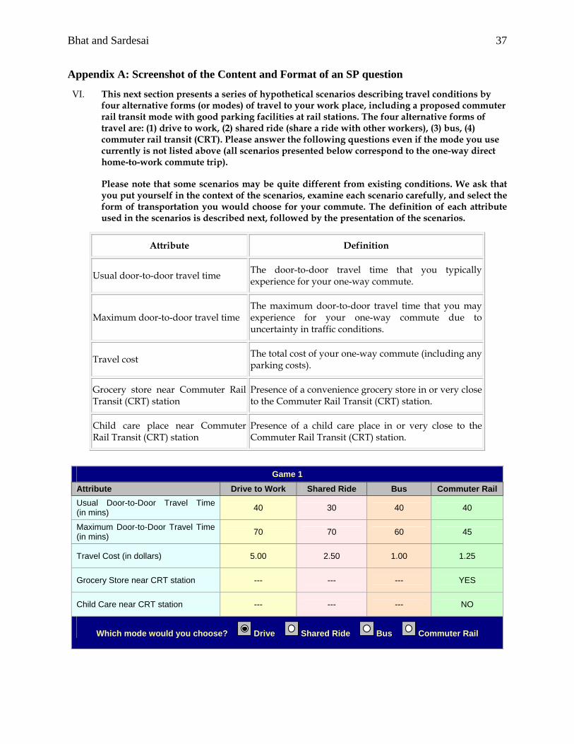
In each of the four SP questions we presented to respondents, five attributes were used to
characterize each alternative: (1) Usual door-to-door commute travel time (in minutes), defined
as the door-to-door commute travel time typically experienced (2) Additional possible door-to-
door commute travel time (minutes) due to uncertainty in traffic conditions, (3) Travel cost (in
dollars), including any parking costs, (4) Availability of a grocery store near the rail station, and
(5) Child care place near the rail station. A screenshot of the precise content and format of a
sample SP question is provided in Appendix A. All the attributes were framed in the context of
the one-way direct home-to-work commute trip. Also, note that in the actual presentation of the
experiments, the second attribute was translated into an effective maximum door-to-door travel
Bhat and Sardesai 9
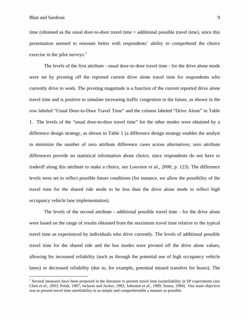
time (obtained as the usual door-to-door travel time + additional possible travel time), since this
presentation seemed to resonate better with respondents’ ability to comprehend the choice
exercise in the pilot surveys.1
The levels of the first attribute - usual door-to-door travel time - for the drive alone mode
were set by pivoting off the reported current drive alone travel time for respondents who
currently drive to work. The pivoting magnitude is a function of the current reported drive alone
travel time and is positive to simulate increasing traffic congestion in the future, as shown in the
row labeled “Usual Door-to-Door Travel Time” and the column labeled “Drive Alone” in Table
1. The levels of the “usual door-to-door travel time” for the other modes were obtained by a
difference design strategy, as shown in Table 1 (a difference design strategy enables the analyst
to minimize the number of zero attribute difference cases across alternatives; zero attribute
differences provide no statistical information about choice, since respondents do not have to
tradeoff along this attribute to make a choice, see Louviere et al., 2000, p. 123). The difference
levels were set to reflect possible future conditions (for instance, we allow the possibility of the
travel time for the shared ride mode to be less than the drive alone mode to reflect high
occupancy vehicle lane implementation).
The levels of the second attribute - additional possible travel time - for the drive alone
were based on the range of results obtained from the maximum travel time relative to the typical
travel time as experienced by individuals who drive currently. The levels of additional possible
travel time for the shared ride and the bus modes were pivoted off the drive alone values,
allowing for increased reliability (such as through the potential use of high occupancy vehicle
lanes) or decreased reliability (due to, for example, potential missed transfers for buses). The
1 Several measures have been proposed in the literature to present travel time (un)reliability in SP experiments (see Chen et al., 2003; Polak, 1987; Jackson and Jucker, 1982; Johnston et al., 1989; Senna, 1994). Our main objective was to present travel time unreliability in as simple and comprehensible a manner as possible.
Bhat and Sardesai 10
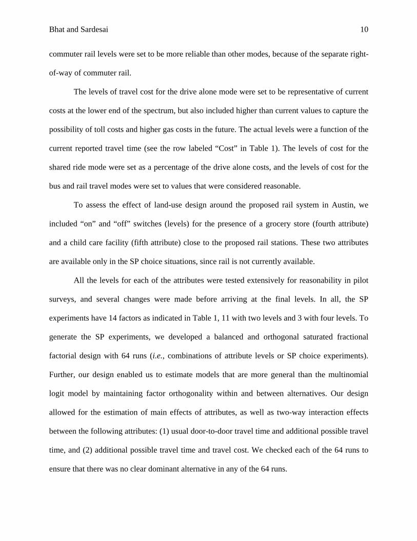
commuter rail levels were set to be more reliable than other modes, because of the separate right-
of-way of commuter rail.
The levels of travel cost for the drive alone mode were set to be representative of current
costs at the lower end of the spectrum, but also included higher than current values to capture the
possibility of toll costs and higher gas costs in the future. The actual levels were a function of the
current reported travel time (see the row labeled “Cost” in Table 1). The levels of cost for the
shared ride mode were set as a percentage of the drive alone costs, and the levels of cost for the
bus and rail travel modes were set to values that were considered reasonable.
To assess the effect of land-use design around the proposed rail system in Austin, we
included “on” and “off” switches (levels) for the presence of a grocery store (fourth attribute)
and a child care facility (fifth attribute) close to the proposed rail stations. These two attributes
are available only in the SP choice situations, since rail is not currently available.
All the levels for each of the attributes were tested extensively for reasonability in pilot
surveys, and several changes were made before arriving at the final levels. In all, the SP
experiments have 14 factors as indicated in Table 1, 11 with two levels and 3 with four levels. To
generate the SP experiments, we developed a balanced and orthogonal saturated fractional
factorial design with 64 runs (i.e., combinations of attribute levels or SP choice experiments).
Further, our design enabled us to estimate models that are more general than the multinomial
logit model by maintaining factor orthogonality within and between alternatives. Our design
allowed for the estimation of main effects of attributes, as well as two-way interaction effects
between the following attributes: (1) usual door-to-door travel time and additional possible travel
time, and (2) additional possible travel time and travel cost. We checked each of the 64 runs to
ensure that there was no clear dominant alternative in any of the 64 runs.

Bhat and Sardesai 11
It is clearly infeasible to present 64 SP choice questions to each respondent, and hence we
developed a block design of 16 sets of 4 SP choice questions. In the block design, each
respondent is presented with 4 SP choice questions. Essentially, we generate a random number
when a respondent visits the on-line web survey and use this random number to select one of the
16 sets of 4 SP questions to present to the respondent.
3. SAMPLE FORMATION AND DESCRIPTION
The data from the completed web surveys were downloaded in ASCII format, and then
imported into SPSS to label and code the variables appropriately. The commute level-of-service
attributes were appended to each individual’s record by extracting this information from
CAMPO’s network skim data. Finally, several cleaning and screening steps were undertaken to
ensure consistency in the records and records with missing network level-of-service, location, or
demographic information were deleted.
The final sample included 679 individuals, 360 of whom made a non-work activity stop
during the survey day and contributed only one choice observation (i.e., the RP choice
observation)2. The remaining 319 individuals contribute five choice observations (1 RP and 4 SP
choice responses). Thus, the combined RP-SP estimation sample comprises a total of 1955
choice occasions (679 RP choice occasions and 1276 SP choice occasions).
In the rest of this section, we discuss mode definition rules (Section 3.1) and modal
availability determinations (Section 3.2), and also present basic descriptive statistics regarding
modal shares in the sample.
2 Only those individuals who did not make any non-work activity stops during the survey day were presented with the SP experiments. This selective presentation scheme was implemented because individuals who made non-work activity stops had to respond to many questions regarding those stops, and our pilot surveys indicated that it was too burdensome for these individuals to also partake in the SP experiments.
Bhat and Sardesai 12
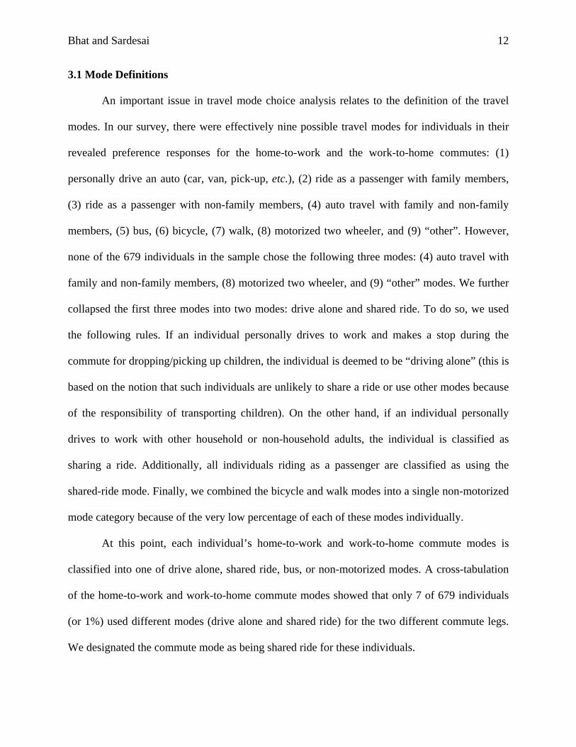
3.1 Mode Definitions
An important issue in travel mode choice analysis relates to the definition of the travel
modes. In our survey, there were effectively nine possible travel modes for individuals in their
revealed preference responses for the home-to-work and the work-to-home commutes: (1)
personally drive an auto (car, van, pick-up, etc.), (2) ride as a passenger with family members,
(3) ride as a passenger with non-family members, (4) auto travel with family and non-family
members, (5) bus, (6) bicycle, (7) walk, (8) motorized two wheeler, and (9) “other”. However,
none of the 679 individuals in the sample chose the following three modes: (4) auto travel with
family and non-family members, (8) motorized two wheeler, and (9) “other” modes. We further
collapsed the first three modes into two modes: drive alone and shared ride. To do so, we used
the following rules. If an individual personally drives to work and makes a stop during the
commute for dropping/picking up children, the individual is deemed to be “driving alone” (this is
based on the notion that such individuals are unlikely to share a ride or use other modes because
of the responsibility of transporting children). On the other hand, if an individual personally
drives to work with other household or non-household adults, the individual is classified as
sharing a ride. Additionally, all individuals riding as a passenger are classified as using the
shared-ride mode. Finally, we combined the bicycle and walk modes into a single non-motorized
mode category because of the very low percentage of each of these modes individually.
At this point, each individual’s home-to-work and work-to-home commute modes is
classified into one of drive alone, shared ride, bus, or non-motorized modes. A cross-tabulation
of the home-to-work and work-to-home commute modes showed that only 7 of 679 individuals
(or 1%) used different modes (drive alone and shared ride) for the two different commute legs.
We designated the commute mode as being shared ride for these individuals.
Bhat and Sardesai 13
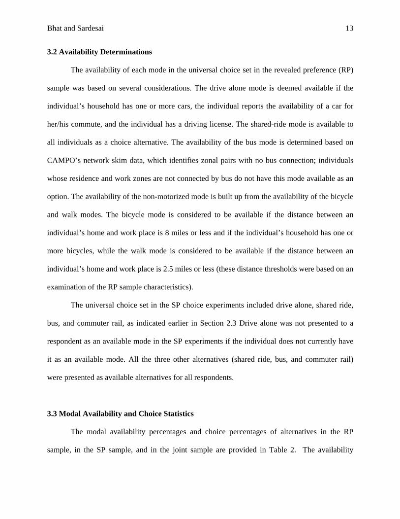
3.2 Availability Determinations
The availability of each mode in the universal choice set in the revealed preference (RP)
sample was based on several considerations. The drive alone mode is deemed available if the
individual’s household has one or more cars, the individual reports the availability of a car for
her/his commute, and the individual has a driving license. The shared-ride mode is available to
all individuals as a choice alternative. The availability of the bus mode is determined based on
CAMPO’s network skim data, which identifies zonal pairs with no bus connection; individuals
whose residence and work zones are not connected by bus do not have this mode available as an
option. The availability of the non-motorized mode is built up from the availability of the bicycle
and walk modes. The bicycle mode is considered to be available if the distance between an
individual’s home and work place is 8 miles or less and if the individual’s household has one or
more bicycles, while the walk mode is considered to be available if the distance between an
individual’s home and work place is 2.5 miles or less (these distance thresholds were based on an
examination of the RP sample characteristics).
The universal choice set in the SP choice experiments included drive alone, shared ride,
bus, and commuter rail, as indicated earlier in Section 2.3 Drive alone was not presented to a
respondent as an available mode in the SP experiments if the individual does not currently have
it as an available mode. All the three other alternatives (shared ride, bus, and commuter rail)
were presented as available alternatives for all respondents.
3.3 Modal Availability and Choice Statistics
The modal availability percentages and choice percentages of alternatives in the RP
sample, in the SP sample, and in the joint sample are provided in Table 2. The availability
Bhat and Sardesai 14
percentage for drive alone is very high, as expected. The availability percentage is 100% for the
shared ride mode because shared ride is always an available mode. The bus and non-motorized
mode availability percentages in the RP sample show that about 43% of commuters have the bus
mode available and about a fifth of commuters have a non-motorized travel mode available. The
availability percentage for the drive alone mode is close to, but not equal to, 100 in the SP
sample because, as indicated earlier, individuals who did not have a vehicle available to them
currently did not have drive alone as an option even in the SP experiments. We presented shared
ride, bus, and rail modes to all respondents in the SP experiments, and thus the availability
percentages of 100 for these modes in the SP sample. The availability shares in the joint sample
are, as expected, between those of the RP and SP samples.
The choice percentages in the RP sample are very close to those from the census journey
to work data and a 2001 random phone survey conducted by CAMPO after accounting for minor
definitional variations between the surveys in the drive alone and shared ride modes3. As
expected, driving alone is the dominant commute mode in the RP sample.
A comparison of the RP and SP mode percentages in Table 2 indicates a clear shift from
the drive alone mode to the other motorized modes. This is, in part, because the SP choice
scenarios involve an increase over the RP scenario in drive alone travel times and costs. Further,
note that, in the SP sample, the bus mode and the rail modes are available to all individuals by
design to maximize the information we are able to extract about the relative tradeoffs between
the level-of-service attributes. Finally, as discussed in Section 6, we are also able to control for
“overstatement” effects in the shift to non-drive modes in the SP experiments.
3 A comparison table of the mode shares from the different surveys is available from the authors.

Bhat and Sardesai 15
4. MODEL FORMULATION
This section discusses the econometric structure of the model used in the analysis as well
as the estimation procedure.
In the usual tradition of random utility maximizing models of choice, we can write the
utility that an individual q associates with an alternative i on choice occasion t as (t may
represent the RP choice occasion or an SP choice occasion):
qitU
( ) ,)1
,, qit
T
sqisRPqsSPqtqqitqqit
q
YxU εδδθα +⎥⎥⎦
⎤
⎢⎢⎣
⎡⎟⎟⎠
⎞⎜⎜⎝
⎛×+′= ∑
=
(1)
where is a vector of observed variables (including variables characterizing the RP and SP
alternative specific constants),
qitx
qα is a corresponding coefficient vector which may vary over
individuals but does not vary across alternatives or time, RPqt ,δ is a dummy variable taking the
value 1 if the tth choice occasion of individual q corresponds to her/his revealed preference
choice and 0 otherwise, RPqtSPqt ,, 1 δδ −= , is another binary variable that takes a value of 1 if
the individual q chooses alternative i at the s
qisY
th choice occasion and 0 otherwise, Tq is the total
number of observed choice occasions for individual q, qθ is the individual-specific effect that
maps the impact of the RP choice of an alternative into the utility evaluation of that alternative in
the SP choice occasions, and qitε is an unobserved random term that captures the idiosyncratic
effect of omitted variables during each choice occasion. qitε is assumed to be independent of qα
and . The reader will note that the second term in Equation (1), representing the effect of the
RP choice on the SP choice, reduces to zero in the utility evaluation for the RP choice occasion.
qitx
Bhat and Sardesai 16
The error term qitε may be partitioned into two components, qitζ and qitzµ′ . The first
component, qitζ , is assumed to be independently and identically Gumbel distributed across
alternatives and individuals for each choice occasion, and also independently (but not
identically) distributed across choice occasions. Specifically, its scale parameter is normalized to
one for the RP choice occasion of an individual, and specified as )/1( λ for the SP choice
occasions of the individual. Such a specification accommodates the scale difference (i.e., the
difference in the variance of unobserved choice-specific factors) between the RP and the SP
choice occasions. The second component in the error term, qitzµ′ , induces heteroscedasticity and
correlation across unobserved utility components of the alternatives at any choice occasion t.
is a vector of observed data, some of whose elements might also appear in the vector .
qitz
qitx µ is a
random multivariate normal vector with zero mean.
Defining ( ) ( )′
⎥⎥⎦
⎤
⎢⎢⎣
⎡⎟⎟⎠
⎞⎜⎜⎝
⎛×′=′′= ∑
=
qT
sqisRPqsSPqtqitqitqqq Yxw
1,,, ,, δδθαβ , and using the error
components decomposition for qitε discussed above, Equation (1) can be re-written as:
qitqitqitqqit zwU ζµβ +′+′= (2)
The coefficient qβ in Equation (2) is individual-specific and, in general, varies across
individuals due to both observed factors (observed individual heterogeneity) and unobserved
factors (unobserved individual heterogeneity). The observed individual heterogeneity can be
incorporated in the usual way by interacting individual-specific variables with the elements of
the vector. Let the distribution of unobserved individual heterogeneity across individuals be
multivariate normal, so that
qitx
qβ is a realization of a random multivariate normally distributed
variable . Let β~ ω be a vector of true parameters characterizing the mean and variance-
Bhat and Sardesai 17
covariance matrix of . Further, let β~ σ be a parameter vector characterizing the variance-
covariance matrix of the multivariate normal distribution of µ .
The probability that individual q will choose alternative i at the tth choice occasion can
then be written as:
),|~()|(
1
)~(
)~(
~ωβσµ
µ µβλ
µβλ
β
dFdFe
eP I
J
zw
zw
qitqjtqjtqt
qitqitqt
∫∑
∫+∞
−∞=
=
′+′
′+′+∞
−∞=
= (3)
where F is the multivariate cumulative normal distribution. The reader will note that the
dimensionality in the integration above is dependent on the number of elements in the µ and qβ
vectors.
The parameters to be estimated in the model of Equation (3) are the σ and ω vectors.
To develop the likelihood function for parameter estimation, we need the probability of each
sample individual's sequence of observed RP and SP choices. Conditional on , the likelihood
function for individual q’s observed sequence of choices is:
β~
( ) ( ) .)|(,~,~1 1∏ ∫ ∏=
+∞
−∞= = ⎥⎥⎦
⎤
⎢⎢⎣
⎡
⎭⎬⎫
⎩⎨⎧
=q
qitT
t
I
i
Yqitq dfPL
µ
µσµµβσβ (4)
The unconditional likelihood function of the choice sequence is:
∫+∞
−∞=
=β
βωβσβσω~
~)|~(),~(),( dfLL qq
(5) ( )∫ ∏ ∫ ∏∞+
−∞= =
∞+
−∞= = ⎪⎭
⎪⎬⎫
⎪⎩
⎪⎨⎧
⎥⎥⎦
⎤
⎢⎢⎣
⎡
⎭⎬⎫
⎩⎨⎧
=β µ
βωβµσµµβ~ 1 1
. ~)|~()|(,~ dfdfPq
qitT
t
I
i
Y
qit
The log-likelihood function is ),(ln),( σωσω qq LL Σ= . The maximization of this
likelihood function with respect to the parameters ω and σ is pursued using a simulation

Bhat and Sardesai 18
approach using Halton draws (the reader is referred to Bhat 2003 for details of simulation
estimation methods). The estimations and computations in the paper were carried out using the
GAUSS programming language on a personal computer.
5. EMPIRICAL ANALYSIS
5.1 Variable Specification
Several types of variables were considered in the commute mode choice model, including
household sociodemographics and residential characteristics, individual sociodemographics and
employment characteristics, commute and midday stop-making characteristics (introduced both
as weekly stop-making variables and stop making variables on the survey day), and land-use
design (presence of grocery/child care places) around commuter rail stations. The level-of-
service variables included total travel time, out-of-vehicle-time, distance, travel cost, and travel
time unreliability (travel time unreliability is defined as the additional travel time that may be
needed to reach the work place because of uncertainty in traffic conditions, and is available only
in the SP choice scenarios). Interaction effects among these variables, as well as interactions of
these variables with variables in other categories (such as unreliability interacted with work
schedule flexibility and the sex of the individual), were also considered.
The final variable specification was determined after systematic testing of several
alternative specifications (in our testing process, we used a statistical significance level of 1.00
for the t-statistic due to the relatively small sample size of commuters). For many variables and
variables interactions, we also considered multiple functional forms. For example, we tested
both linear and non-linear forms (spline and dummy variable functional form) for the effect of
Bhat and Sardesai 19
household income, personal income, and age, The entire specification process was guided by
intuitive considerations and parsimony in representing variable effects.
A final note before moving on to the empirical results. To determine if the variable
effects from the RP and SP data should or should not be restricted to be the same in the joint RP-
SP formulation, we estimated an unrestricted “joint RP/SP multinomial logit (MNL)” model with
a completely different set of coefficients on variables in the RP and SP choice processes, except
for the cost coefficient, which was constrained to be the same to identify the RP-SP scale
difference. But this model was not statistically superior to the joint RP/SP MNL model that
constrained the coefficients on the variables to be the same in the RP and SP data, except for
alternative constant differences in the RP and SP choice processes. Furthermore, the difference
in each of the non-cost variable coefficients between the unrestricted and restricted versions of
the joint RP/SP MNL model was not statistically significant. Thus, we accepted the hypothesis
that the RP and SP choice data were representing the same underlying preference and trade-off
structure in all subsequent estimations.
5.2 Empirical Results
5.2.1. Model Structure
A number of different model structures were estimated in our analysis. The final
preferred structure corresponded to one in which there was no statistically significant impact of
the RP choice of an alternative on the utility evaluation of that alternative in the SP choice
occasions (that is, 0=qθ for all individuals q in Equation 1) and no statistically significant
heteroscedasticity/correlation across unobserved utility components of the alternatives at the
choice occasion level (that is, the elements of σ , the vector characterizing the variance-
Bhat and Sardesai 20
covariance matrix of µ in Equation 2, are all zero). This final preferred structure takes the form
of a mixed logit model that corresponds to a random coefficients MNL model with scaling
between the RP and SP choice settings. In this random coefficients model, we used a normal
mixing distribution to represent the profile of the variation among individuals in their preference
heterogeneity. We held the price parameter fixed for stability (see also Revelt and Train, 1998
and Brownstone and Small, 2005). For the random coefficients on the travel time and reliability
variables, we tested both the normal and log-normal distributions, and found the normal
distribution to provide better fit measures. The reader will note that the normal distribution
implies that some individuals will have a positive response coefficient to travel time and
unreliability. As we will see later, however, less than 0.5% of commuters are assigned such a
positive coefficient on travel time. In any case, there is some evidence to suggest that some
commuters actually place a positive utility on commute travel time (see Mokhtarian and
Redmond, 2001). With regard to reliability, several earlier research works have indicated that
some travelers may be risk-inclined (see Brownstone and Small, 2005; Senna, 1994).
5.2.2. Variable Effects
The final specification results of the commute mode choice model are presented in Table
3. In the following sections, we discuss the effect of variables by variable category.
5.2.2.1 Household Sociodemographics and Residential Characteristics Several household
sociodemographics and residential characteristics were tested in the model, but only those related
to the number of motorized vehicles per licensed driver and household income appeared in the
final specification. The results indicate that, as expected, individuals in households with a high
Bhat and Sardesai 21
number of motorized vehicles per licensed adult are likely to choose the drive alone mode, since
there is less competition for cars. The coefficients on the income variable show that individuals
from high income-earning households are unlikely to use the bus or non-motorized travel modes.
Interestingly, we did not find any such negative income effect for the commuter rail transit (rail)
mode. This may suggest that, while individuals from high income households perceive traveling
on the bus as not being consistent with their social status, they may have a more positive image
of rail. It should be noted that in addition to the linear effect presented in the table, non-linear
spline effects of household income were also explored, but did not improve data fit significantly.
Additionally, an approach that assigned individuals to discrete income categories was also
examined, but did not provide better results than the linear income form.
5.2.2.2 Individual Sociodemographics and Employment Variables Among the individual
sociodemographic and employment variables, the effect of personal income (as a fraction of total
household income) indicates that high income earners in the household avoid the shared ride and
bus modes. Again, there is no negative impact of personal income on the rail mode, suggesting
that rail may not only conjure up a more positive image than bus, but may also be viewed by
high income earners as being preferred to shared ride from a privacy/independence standpoint.
The workplace employment density variables has a positive impact on the use of the transit
modes (bus and rail), reflecting perhaps the tension and anxiety associated with driving and
parking in high density areas. Also commuters may be reluctant to use non-motorized modes in
a high employment density zone due to safety considerations associated with high motorized
traffic volumes.
Bhat and Sardesai 22
5.2.2.3 Level of Service Measures We allow the response to sensitivity to level of service
measures to vary across individuals due to both observed and unobserved individual attributes
(except for the cost coefficient, which is allowed to vary based on observed individual attributes,
but not unobserved individual attributes).
The mean coefficients on the level of service measures in Table 3 show the expected
negative effects of total travel time, cost, and travel-time reliability for motorized modes and the
negative influence of commute distance on non-motorized mode choice. Interestingly, we did
not find any systematic response variations across individuals (i.e., observed individual
heterogeneity) to the time, cost, and commute distance measures (and, thus, there are no
interactions of individual attributes with these level of service variables in Table 3). However,
the results indicate that there is a difference in sensitivity to travel time unreliability (at about a
0.1 level of significance) based on whether or not a person’s work arrangement is inflexible (for
purposes of the current analysis, an individual’s work arrangement is considered inflexible if s/he
reports that it is “very difficult” or “difficult” to arrive at work 15-30 minutes late in the
morning). The results show that commuters with an inflexible work schedule value reliability
more than commuters with a flexible work schedule, consistent with the notion that unreliability
has a scheduling cost. However, even for commuters with a flexible work schedule, unreliability
has a mean negative effect due to a travel time uncertainty cost. Unlike Lam and Small, 2001,
we did not find any statistically significant response variations to unreliability based on the sex
of the commuter.
The standard deviations of the parameters on total travel time and travel time unreliability
are statistically significant, indicating the presence of response heterogeneity. The estimated
mean coefficient on the travel time variable, along with the estimated standard deviation of the
Bhat and Sardesai 23
time sensitivity across individuals, implies a negative effect of travel time for almost all
commuters. The normal distribution for heterogeneity will necessarily imply a positive
coefficient for some individuals; in the current analysis, this is estimated to be the case for less
than 0.5% of individuals. However, the results indicate that travel time unreliability is positively
valued by 27% of commuters with a flexible work schedule and by 13% of commuters with an
inflexible work schedule. Clearly, these findings show that Austin area commuters are
homogenous in valuing travel time negatively in their mode choice decisions, but are more
heterogeneous in their views on whether or not travel time unreliability is undesirable4.
However, it should be noted that there is higher homogeneity regarding the undesirable view of
travel time unreliability within the group of inflexible work schedule commuters relative to the
group of flexible work schedule commuters.
5.2.2.4 Commute and Midday Stop-making Characteristics Among the commute and midday
stop-making characteristics that we considered, only three variables had an impact on travel
mode choice. These correspond to “make a commute stop on one or more days of the work
week”, “make midday stops on some days of the work week”, and “make midday stops on every
day of the work week”. The positive signs of the alternative-specific parameters on the first
variable is a clear reflection that commuters have a preference for the auto mode of travel
relative to the transit and non-motorized modes if they make commute stops on one or more days
of a week. Similarly, the positive signs on the midday stop variables show a strong inclination to
drive alone, with the effect being stronger if the individual makes midday stops on every day of
the work week. These results highlight the need to consider commute and midday stop-making
in travel mode choice modeling. 4 This result needs further exploration to better understand the cause of the positive impact of unreliability.
Bhat and Sardesai 24
Overall, the results provide support for the view that mixed use development at the work
place has the potential to facilitate mode switching from the auto modes to the non-auto modes.
Also, studies that do not consider the impact of commute and midday stop-making on commute
mode choice will overestimate the shift away from the auto modes to transit and non-motorized
modes in response to auto-use disincentive and non-auto use incentive strategies.
Several important observations may also be made based on the stop-making variables that
do not appear in Table 3 (these variables were found to be statistically insignificant in earlier
specifications). First, the number of days with one or more commute stops is not relevant in
commute mode choice; what is relevant is only whether or not an individual makes commute
stops on one or more days. Second, after controlling for whether or not commuters make a stop
on one or more days of the week, there is no remaining effect of stops on the survey day. Thus,
the results indicate that the effect of commute and midday stop-making on commute mode
choice is manifested at a weekly level, not a daily basis. That is, individuals who do not make
commute or midday stops every day (but make such stops at least once a week) are likely to
drive alone on each day of the week. A couple of possible reasons for this are that (1)
individuals do not decide in advance on the precise day for participation in non-work stops, and
thus want the flexibility to pursue these stops on any day of the week, (2) individuals may make
commute and/or midday stops on only one or a few clearly identified days of the week (for
example, dropping a small child at preschool only on Mondays and Wednesdays), but drive to
work on all days of the week due to habituation. In any case, our results suggest that studies that
consider the effect of stop-making on commute mode choice at a daily level may be myopic in
their perspective and may miss the broader stop-making context in which commute choice
decisions are made. This finding has important policy implications, since the extent of weekly
Bhat and Sardesai 25
commute and midday stop-making is much more prevalent than daily commute and midday stop-
making. For example, from our Austin sample, we find that 83.9% (64.7%) of commuters make
one or more commute (midday) stops during the week, while only 31.4% (30.8%) of commuters
make one or more commute (midday) stops on the survey day (these are weighted statistics of
our sample to reflect the commuter population in Austin). Thus, earlier mode choice studies that
consider the effect of stop-making only at a daily level are likely to provide overly optimistic
projections of the impact of Transportation Control Measures (TCMs). Finally, in our empirical
analysis, we found that the purpose of commute or midday stops on the survey day did not have
any bearing on commute mode choice.
5.2.2.5 Land Use Design Attributes Around Rail Stations The effect of the land use design
attributes indicates that the presence of a grocery store around rail stations acts as an impetus for
rail mode-use, among those individuals who pursue one or more commute stops during the week
(again, we did not find any daily commute stop-making interaction effects with the presence of a
grocery place near rail stations).
Interestingly, there was no statistically significant effect of a child care center near the
rail station on rail choice. We also interacted this variable with an indicator variable for whether
the commuter has a small child and whether the individual made a child care stop on the survey
day, but these effects were also not significant. Third order interaction effects of the above
variables with the sex of the individual were also considered, but also turned out to be
insignificant. The absence of the effect of a child care center around rail stations on rail mode
choice may suggest that parents do not consider rail stations to be appropriate locations, from a
safety and noise standpoint, for child care centers.

Bhat and Sardesai 26
5.2.2.6 Alternative-Specific Constants and Scale Factor The mean value of the RP and SP
constants do not have any behavioral interpretations because of the presence of several
continuous exogenous variables in the specification. However, it is interesting to note the higher
positive constants on the shared ride and bus modes in the SP sample relative to the RP sample.
This suggests that individuals are overstating their tendency to shift to the non-drive modes in
the SP experiments. By using the RP constants in prediction, the analyst is able to recognize and
adjust for the overstatement in the use of the non-drive modes in the SP responses (see Section 6
for more details). The reader will also note that the RP alternative specific constant for the bus
mode was not distinguishable from zero up to the fourth decimal place.
The estimated standard deviations characterizing the unobserved heterogeneity
distribution for the constant are highly significant. Thus, there appears to be considerable
individual-level heterogeneity in intrinsic preferences for the different alternatives.
Finally the RP to SP scale factor is much higher than, and significantly different from, 1,
indicating that the error variance in the SP choice context is much lower than in the RP choice
context. Interestingly, when unobserved heterogeneity is ignored, the RP to SP scale factor is
significantly smaller than 1, incorrectly indicating that the error variance in the SP choice context
is much higher than in the RP choice context (see also Bhat and Castelar, 2002 and Daniels and
Hensher, 2000 for a similar result).
5.3 Implied Money Values and Data Fit Measures
The implied mean money values of travel time (VOT) and reliability (VOR) can be
obtained in a straightforward manner from the coefficients on time, reliability, and cost. In Table
Bhat and Sardesai 27
4, we present the VOT and VOR values, as well as the data fit measures, for the joint SP-RP
mixed MNL model with unobserved heterogeneity (whose model coefficients were presented in
the previous section) and three other precursor models: (1) the RP sample MNL, (2) the SP
sample MNL, and (3) the joint RP-SP MNL.
A comparison of the VOT values across the models (see first row of Table 4) indicates
that the VOT value is higher from the RP-sample MNL compared to the SP-sample MNL. This
is consistent with the findings from earlier studies such as Ghosh (2001) and Small et al. (2005).
However, unlike these earlier studies where the RP VOT was about 2-3 times larger than the SP
VOT, we find the VOT estimates from the RP and SP samples to be much more comparable.
The SP-sample VOT is slightly lower than the VOT estimates from the joint RP-SP MNL and
the joint RP-SP mixed MNL with unobserved individual heterogeneity. Surprisingly, the
addition of unobserved individual heterogeneity has almost no impact on mean VOT estimates in
the current empirical context, unlike the studies of Bhat and Castelar (2002) and Daniels and
Hensher (2000).
The VOR estimates are estimable from the SP and joint RP-SP samples, but not from the
RP sample (while we obtained a reported measure of the maximum time it took for the commute
in the RP questions, we have this measure only for the chosen commute mode). The estimates
indicate that the VOR for commuters with an inflexible work schedule is about twice that for
commuters with a flexible schedule. The results also reveal a dramatic drop in the VOR
estimates when unobserved individual heterogeneity is added. Thus, while the VOT estimates
are relatively unaffected by adding heterogeneity, our results show that ignoring unobserved
heterogeneity leads to inflated money values of reliability in the current empirical setting.
Bhat and Sardesai 28
We next turn to a comparison between the VOT and VOR estimates. Our estimates from
the SP-sample MNL and the joint RP-SP MNL model indicate that reliability is valued at
roughly 60% of the usual travel time for commuters with a flexible work arrangement, and about
120% of the usual travel time for commuters with inflexible work schedules (the latter estimate
is comparable to those obtained from several earlier studies, including Noland and Small, 1995;
Small et al., 1999; Rohr and Polak, 1998; and Small et al., 2005)5. However, the estimates from
the joint RP-SP mixed MNL model with unobserved individual heterogeneity, which is the
preferred specification in the current empirical analysis, reflects a much lower mean VOR to
mean VOT ratio. Specifically, reliability is valued at about 27% of the usual travel time for
commuters with a flexible work arrangement and at 50% of the usual travel time for commuters
with an inflexible work arrangement. These estimates are even lower than the VOR/VOT
percentage of 79% obtained by Black and Towriss (1993) and the VOR/VOT percentage of 52%
obtained by Lam and Small (2001) for male commuters.
A clear indication from our results is that the VOR value, and the VOR to VOT ratio, can
be highly sensitive to model specification. In our empirical context, the VOR ratio is about 50%
lower in the case when unobserved individual heterogeneity is considered compared to when it is
not. While it would not be appropriate to directly compare the VOR to VOT ratios from this
study and earlier studies (due to differences in the way reliability is measured, RP vs. SP data,
cultural and locational differences, and the choice context under study), there is a suggestion that
some earlier studies may have overestimated the VOR to VOT ratio because of ignoring
unobserved individual heterogeneity effects.
5 The reader is referred to Brownstone and Small (2005) and Bates et al. (2001) for reviews of VOT and VOR from earlier studies.
Bhat and Sardesai 29
The fit measures between the RP-sample MNL and SP-sample MNL are not strictly
comparable because of the different samples and different choice sets. The joint RP-SP MNL
shows a rather low 2ρ value at 0.047. The differences in fit in Table 4 between the joint RP-SP
MNL and the joint RP-SP mixed MNL with unobserved individual heterogeneity is dramatic,
increasing from 0.047 to 0.204 (the likelihood ratio test corresponding to a comparison of these
two models is 570.3, which is larger than the chi-squared statistic with 6 degrees of freedom at
any reasonable level of significance). This indicates the importance of including heterogeneity
from a data fit perspective.
6. POLICY SIMULATIONS
6.1. Background and Preparatory Steps
As a precursor to applying the model for policy evaluation, we need to obtain the
appropriate RP constants to apply in prediction to ground our forecasts on reality, rather than use
the SP constants that show signs of overstatement of the use of non-drive alone modes. In the
estimation process, the RP constants are estimated for the shared ride, bus, and non-motorized
modes. However, there is no RP constant estimated for the rail mode. Further, the RP constants
from estimation for the shared ride, bus, and non-motorized modes are also not directly
transferable for prediction because of two reasons: (1) The RP sample in estimation, though
representative in the mode choices, is not representative in the commuter characteristics (on the
other hand, for policy analysis, we need a representative sample in both exogenous variables and
current mode shares), and (2) The estimated RP constants (from the joint RP-SP estimation) do
not include unreliability in the RP scenario (in the rest of this section, we will use the terms “RP

Bhat and Sardesai 30
and SP constants” to refer to the mean values of these constants; the standard deviations of these
constants are immediately available from the joint RP-SP estimation in Table 3).
To accommodate the issues raised above, we pursued four broad preparatory steps. First,
we obtained an equivalent RP utility differential in overall intrinsic preference between the rail
and bus modes using the estimated SP rail and bus utility functions. Appendix B.1 discusses the
procedure, which is not as straightforward as simply using the difference between the SP rail and
bus constants (due to the presence of continuous variables in the utility functions). The estimated
RP utility differential between the rail and bus modes from implementing the procedure in
Appendix B.1 is +1.10. Dividing this by the coefficient of travel time, we find a rail “travel time
bonus” of about 20 minutes relative to the bus mode. That is, all other things being equal
between the bus and rail modes, individuals will prefer the rail mode even if the rail travel time
is more than the bus travel time by up to 20 minutes. While this rail bonus is relatively high
compared to the current bus travel time of about 53 minutes, it is not unreasonable.
Second, we obtained a sample that is representative in both exogenous variables and
current mode choices (drive alone, shared-ride, bus, and non-motorized modes). To do so, we
weighted the RP sample based on a multivariate distribution of race, income earnings, and sex
for the 3-county Austin area using the 2000 census of population and housing survey file. Once
we weighted on these three variables, the distribution became representative for several other
exogenous variables and commute-related characteristics. However, the mode choice shares
were slightly higher than the market shares for the bus mode and the non-motorized modes. To
achieve current mode choice market share representation as well as population representation,
we adopted an iterative proportional fitting procedure to get convergence along all dimensions.
Bhat and Sardesai 31
Third, we estimated the appropriate RP constants to use in prediction for the shared-ride,
bus, and non-motorized modes by using the representative sample developed in the second step,
as well as making appropriate assumptions about unreliability values for these modes. Appendix
B.2 describes this procedure.
Finally, we applied the equivalent RP utility differential in overall intrinsic preference
between the rail and bus modes (as estimated in the first step) to the bus utility function from the
third step to obtain an effective RP constant for rail (again, this is not as straightforward as
applying the rail to bus RP utility differential in overall intrinsic preference to the bus RP
constant obtained in the third step). Appendix B.3 presents the procedure.
At the end of these steps, we have the appropriate RP constants for all the five modes
(including rail), as well as a representative sample to undertake policy analysis. We are then able
to test all policies that influence one or more exogenous variables. In the current paper, we
provide a small sampling of the kinds of analyses that can be pursued. Specifically, we first
consider the case when commuter rail transit (rail) is available as an option and then add the
effect of highway tolls. All simulations are conducted using a sample enumeration procedure.
The next two sections discuss the two policy cases considered in this paper.
6.2 Effect of Commuter Rail as an Available Alternative
We assume that the rail design includes grocery stores around rail stations and that rail is
available for a randomly selected sample of 50% of individuals who have bus as an available
option (in reality, the availability of the rail system for each individual commuter will depend on
the precise alignment of the rail system). In evaluating the effect of the rail mode, we estimate
the impact on overall mode shares as well as on segments of the population defined by (1)
Bhat and Sardesai 32
availability of rail as an alternative, (2) whether or not individuals make one or more commute
stops during the week, and (3) whether or not individuals make midday stops during the week.
This disaggregate analysis is pursued to illustrate the impact of availability of rail, commute
stops, and midday stops on commute mode choice.
Table 5 presents the results. The column labeled “Mode Shares” indicates how the
overall mode shares change after introduction of a commuter rail transit (rail) mode. As
expected, there is a decrease in the shares of all existing modes, with the proportionate draw
away from the bus and non-motorized modes being higher than the drive alone and shared ride
modes (this is a consequence of the random coefficient on the travel time variable; since the bus
and non-motorized modes have high travel times like the rail alternative, there is a higher level
of sensitivity generated at the individual commuter level between these three alternatives).
The column labeled “Mode Shares by Rail Availability” shows the very important effect
of rail availability in the choice set on rail mode shares. In particular, in the segment with rail as
an available alternative, the share of drive alone is much lower than for the segment without rail
availability. The shares of bus and walk modes are also higher for the “rail available” segment
because of the fact that rail availability is pinned to transit availability in our simulations. Thus,
bus is always also available for each individual in the “rail available” segment. Further, the non-
motorized shares are also higher for this segment because transit is prevalent in high density
areas, where walking is more likely to be feasible.
The column entitled “Mode Shares by Weekly Commute Stop-making” indicates the
important effect of weekly commute stop-making on commute mode choice. Specifically,
commuters making commute stops on one or more days of the week are highly predisposed to
driving alone. Similarly, the results reveal the substantial influence of midday stop-making on
Bhat and Sardesai 33
commute mode choice. Commuters making midday stops on every day of the week are
particularly unlikely to consider the transit modes or a non-motorized mode.
The results above reinforce the empirical findings discussed in Section 5. Three
particularly important conclusions may be drawn from Table 5. First, commuter rail has some
potential to decrease the share of driving alone, but is likely to draw more proportionate shares
from the bus and non-motorized modes than the drive alone and shared ride modes. Of course,
our analysis does not consider the access mode to a proposed commuter rail, an issue that needs
additional careful attention. Second, rail availability to individual commuters is critical in
determining the reduction in drive alone mode share. While this is intuitively obvious, our
analysis quantifies the important effect of rail availability. The initial alignment of the rail route
should be carefully designed based on the residence and workplaces of Austin area commuters so
that rail becomes a viable alternative for as large a fraction of the population as possible. The
other side of this finding is the caution that one should not expect substantial shifts in drive alone
mode shares after the implementation of a “starter” rail system. The real benefits of a rail system
from a traffic congestion standpoint will likely accrue only when the proposed rail system is
expanded sufficiently to serve a reasonable fraction of the commuter population. Third, policies
that reduce the need for commute and midday stop-making (such as good land-use mixing at the
workplace) have the potential to reduce car dependency for the commute.
6.3 Impact of Highway Tolls on Commute Mode Shares
We examine the impact of highway tolls on commute mode shares by “imposing” an
additional $1.00 toll for the use of all the major highways in the Austin area for individuals who
drive alone (it is important to emphasize that we are not proposing such a blanket tolling system,

Bhat and Sardesai 34
but simply demonstrating the potential of our model to provide forecasts in response to tolls).
We are able to pursue such an analysis because our survey collected information on the use of
the following major highways: Mopac, IH-35, US-183, US-360, US-71, US-290, and FM-2222.
Thus, in the toll policy simulations, we increase the travel cost by drive alone for all individuals
who use the major highways listed above. 6
In addition to a $1.00 toll, we also examine the impact of a $2.00 toll on all major
highways. In each case, we estimate the mode share impact within the subgroup of highway
users and highway non-users.
Table 6 presents the results. In the “No Toll Case”, a comparison of the columns labeled
“overall” for the “No Toll Case”, the case with a “$1.00 toll”, and the case with a “$2.00 toll”
shows the expected downward trend of the drive alone mode share as the toll increases. Much of
this shift is to the shared ride mode rather than the transit or non-motorized modes. The
breakdown by highway and non-highway users for the “no toll case” shows higher drive alone
and shared ride shares, and lower transit and non-motorized mode shares, for highway users
relative to non-highway users. An analysis of the data revealed that this is because of the better
level of service of the car modes (compared to non-car modes) for highway users, as well as
because of the lower availability of the non-car modes for highway users. A comparison of the
columns labeled “highway users” across the three different toll cases suggests a drop of about
2.5% in the drive alone mode share on highways for each $1.00 increase in toll. There are no
mode share changes for non-highway users because these commuters are not affected by the toll.
6 Note that, in our policy simulations, we are assuming a $1.00 toll regardless of the number of major highways used during the commute.
Bhat and Sardesai 35
7. CONCLUSIONS
This paper has estimated a commute mode choice model, incorporating the effects of
midday and commute stop making as well as travel time unreliability. Heterogeneous generic
preferences across individuals for travel modes and varying sensitivities to level-of-service
attributes are explicitly accommodated in the analysis, which is based on fusing revealed
preference (RP) and stated preference (SP) data. A mixed logit framework that accommodates
the scaling difference between the RP and SP data is used in the modeling. The mixed logit
model is estimated using a simulated maximum likelihood (SML) approach with Halton draws.
The empirical analysis is undertaken in the context of the Austin metropolitan area in
Texas. There are several important findings from our results. First, stop-making during the
commute and the midday have a very important effect on commute mode choice. Models that do
not recognize this influence are likely to provide overly optimistic projections of the effect of
transportation control measures (TCMs). Second, there is a strong indication that stop-making at
the weekly level is the determining factor in commute mode choice. After accommodating the
weekly level of stop-making, there is no impact of daily stop-making on the commute mode
chosen. This result even further cautions against the use of traditional trip-based mode choice
models for TCM analysis. Third, the results indicate that travel time unreliability is an important
level-of-service attribute that needs to be considered in travel analysis. The influence of travel
time unreliability is particularly pronounced for commuters with an inflexible work schedule.
Fourth, the model specification adopted in the analysis impacts the valuation of reliability
relative to travel time. Our results suggest that the value of reliability (VOR) is overstated when
unobserved individual heterogeneity is ignored, as has been done by some earlier studies. While
this conclusion cannot be generalized to all empirical contexts, it is clear that it is critical to test
Bhat and Sardesai 36
for the presence of preference and taste variations across individuals for the accurate assessment
of policy actions. Fifth, the results show that a well-designed commuter rail transit system may
have some potential to shift commuters from driving alone to other modes. The extent of this
shift is predicated on the careful alignment of the rail system so it is available as a viable option
to a reasonable fraction of current commuters. Further, the reliability, travel time, travel costs,
and presence of grocery shops near rail stations also have an important impact on rail use.
However, it is important to pursue a more in-depth simulation of possible rail service scenarios,
and a rigorous and comprehensive cost-benefit analysis of the rail system to better understand the
full impacts and viability of a potential rail system for Austin.
ACKNOWLEDGEMENTS
This research was funded by the U.S. Department of Transportation through the
Southwest Region University Transportation Center. The authors would like to thank Allison
Lockwood, Harsha Nerella, Aswani Yeraguntla, and Aruna Sivakumar for help with the web
survey design, testing, and data extraction. Several other transportation graduate students also
assisted in disseminating information regarding the survey. The authors are indebted to the
Clean Air Force of Central Texas (especially Wendy Willingham and Deanna Altenhoff) and
Nustats, Inc. (Johanna Zmud and Mia Zmud) for their support of this research effort. Lisa
Macias helped with typesetting and formatting. The comments of Professor Kenneth Small and
an anonymous reviewer on an earlier version of the paper helped improve the presentation.
Finally, the first author would like to dedicate his part of the research efforts to his Father, Dr.
Ramalinga Bhat, who passed away in May 2005.
Bhat and Sardesai 37
Appendix A: Screenshot of the Content and Format of an SP question
VI. This next section presents a series of hypothetical scenarios describing travel conditions by four alternative forms (or modes) of travel to your work place, including a proposed commuter rail transit mode with good parking facilities at rail stations. The four alternative forms of travel are: (1) drive to work, (2) shared ride (share a ride with other workers), (3) bus, (4) commuter rail transit (CRT). Please answer the following questions even if the mode you use currently is not listed above (all scenarios presented below correspond to the one-way direct home-to-work commute trip).
Please note that some scenarios may be quite different from existing conditions. We ask that you put yourself in the context of the scenarios, examine each scenario carefully, and select the form of transportation you would choose for your commute. The definition of each attribute used in the scenarios is described next, followed by the presentation of the scenarios.
Attribute Definition
Usual door-to-door travel time The door-to-door travel time that you typically experience for your one-way commute.
Maximum door-to-door travel time The maximum door-to-door travel time that you may experience for your one-way commute due to uncertainty in traffic conditions.
Travel cost The total cost of your one-way commute (including any parking costs).
Grocery store near Commuter Rail Transit (CRT) station
Presence of a convenience grocery store in or very close to the Commuter Rail Transit (CRT) station.
Child care place near Commuter Rail Transit (CRT) station
Presence of a child care place in or very close to the Commuter Rail Transit (CRT) station.
Game 1
Attribute Drive to Work Shared Ride Bus Commuter Rail Usual Door-to-Door Travel Time (in mins) 40 30 40 40
Maximum Door-to-Door Travel Time (in mins) 70 70 60 45
Travel Cost (in dollars) 5.00 2.50 1.00 1.25
Grocery Store near CRT station --- --- --- YES
Child Care near CRT station --- --- --- NO
Which mode would you choose? Drive Shared Ride Bus Commuter Rail
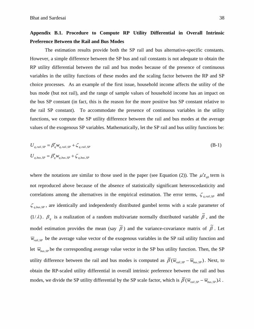
Bhat and Sardesai 38
Appendix B.1. Procedure to Compute RP Utility Differential in Overall Intrinsic
Preference Between the Rail and Bus Modes
The estimation results provide both the SP rail and bus alternative-specific constants.
However, a simple difference between the SP bus and rail constants is not adequate to obtain the
RP utility differential between the rail and bus modes because of the presence of continuous
variables in the utility functions of these modes and the scaling factor between the RP and SP
choice processes. As an example of the first issue, household income affects the utility of the
bus mode (but not rail), and the range of sample values of household income has an impact on
the bus SP constant (in fact, this is the reason for the more positive bus SP constant relative to
the rail SP constant). To accommodate the presence of continuous variables in the utility
functions, we compute the SP utility difference between the rail and bus modes at the average
values of the exogenous SP variables. Mathematically, let the SP rail and bus utility functions be:
SPrailqSPrailqqSPrailq wU ,,,,,, ζβ +′= (B-1)
SPbusqSPbusqqSPbusq wU ,,,,,, ζβ +′=
where the notations are similar to those used in the paper (see Equation (2)). The qitzµ′ term is
not reproduced above because of the absence of statistically significant heteroscedasticity and
correlations among the alternatives in the empirical estimation. The error terms, SPrailq ,,ζ and
SPbusq ,,ζ , are identically and independently distributed gumbel terms with a scale parameter of
)/1( λ . qβ is a realization of a random multivariate normally distributed variable , and the
model estimation provides the mean (say
β~
β ) and the variance-covariance matrix of . Let β~
SPrailw , be the average value vector of the exogenous variables in the SP rail utility function and
let SPbusw , be the corresponding average value vector in the SP bus utility function. Then, the SP
utility difference between the rail and bus modes is computed as )( ,, SPbusSPrail ww −β . Next, to
obtain the RP-scaled utility differential in overall intrinsic preference between the rail and bus
modes, we divide the SP utility differential by the SP scale factor, which is λβ )( ,, SPbusSPrail ww − .
Bhat and Sardesai 39
Appendix B.2. Procedure to Obtain RP Constants for Shared-Ride, Bus, and Non-
Motorized Modes for Use in Prediction
The third preparatory step for policy analysis is to obtain the RP constants to use in
prediction for the shared-ride, bus, and non-motorized modes. The original RP constants
obtained from the joint RP-SP estimation are not appropriate for the reasons mentioned in the
text. After obtaining a weighted representative sample in both the mode choices and commuter
characteristics (the second preparatory step), we need to estimate appropriate RP constants that
include the unreliability variable in the RP setting. Accordingly, we set the unreliability values to
be 20 minutes for the drive alone, shared ride, and bus modes, based on the reported maximum
minus typical travel times from the survey. The unreliability value for the non-motorized mode
category is set to zero. Next, we estimated a new RP model with the four current modes (drive
alone, shared ride, bus, and non-motorized modes) using the weighted representative sample
generated in the second preparatory step, fixing the coefficients on all non-constant variables at
the joint RP-SP estimated values, and estimating new RP constants for the shared-ride, bus, and
non-motorized modes. At the end of this step, we have all the RP coefficients (and their
distributions) for the drive alone, shared-ride, bus, and non-motorized modes.
Appendix B.3. Procedure to Obtain Rail RP Constant for Use in Prediction
The final step before using the estimated model for policy analysis is to transfer the RP-
scaled SP utility difference between the rail and bus utility functions (see Appendix B.1) to
obtain the RP constant for the rail mode, again accommodating the range of exogenous variables
in the RP situation. To do so, we need “RP” estimates of the rail level of service (these can be
viewed as the potential service levels that are planned for the new rail service). In the current
paper, we equated bus times to rail times for each individual in the weighted representative
sample, and set the cost of rail to be twice that of the bus mode. Further, since the rail mode has
a separate right of way, we set the rail unreliability value to be 10 minutes (half of the
unreliability values for the other motorized modes). Next, we computed the average RP utility of
the bus mode at the average of the exogenous variable values, and did the same for the rail mode
(without the rail constant, since this is not known yet). Finally, we estimated the RP constant for
the rail mode such that the utility differential between the average RP utilities of the rail and bus
modes is +1.10. The effective RP constant for the rail mode turned out to be -0.45.

Bhat and Sardesai 40
REFERENCES Abkowitz, M.D. (1980) The impact of service reliability on work travel behavior. Ph.D.
dissertation, Department of Civil Engineering, Massachusetts Institute of Technology, Cambridge, MA.
Abkowitz, M.D. (1981). Understanding the effect of transit service reliability on work-travel
behavior. Transportation Research Record, 794, 33-41. Adiv, A. (1983) The structure of the work trip based on analysis of trip diaries in the San
Francisco Bay area. In Recent Advances in Travel Demand Analysis, edited by S. Carpenter and P. Jones, Aldershot, Gower, England.
Bates, J., Polak, J., Jones, P., and Cook, A. (2001) The valuation of reliability for personal travel.
Transportation Research Part E, 37(2), 191-229. Bhat, C.R. (1998) Accommodating variations in responsiveness to level-of-service variables in
travel mode choice modeling. Transportation Research Part A, 32(7), 495-507. Bhat, C.R. (2003) Simulation estimation of mixed discrete choice models using randomized and
scrambled Halton sequences. Transportation Research Part B, 37(9), 837-855. Bhat, C.R. (2004) Austin commuter survey: findings and recommendations. Technical Report,
Department of Civil, Architectural & Environmental Engineering, The University of Texas at Austin. http://www.ce.utexas.edu/prof/bhat/reports/austin_commuter_survey_report.doc
Bhat, C.R., and Castelar, S. (2002) A unified mixed logit framework for modeling revealed and
stated preferences: Formulation and application to congestion pricing analysis in the San Francisco Bay area. Transportation Research Part B, 36(7), 593-616.
Bhat, C.R., and Singh, S.K. (2000) A comprehensive daily activity-travel generation model
system for workers. Transportation Research Part A, 34(1), 1-22. Bhat, C.R., and Zhao, H. (2002) The Spatial Analysis of Activity Stop Generation.
Transportation Research Part B, 36(6), 557-575. Black, I.G., and Towriss, J.G. (1993) Demand Effects of Travel Time Reliability. Cranfield
University, Cranfield, U.K. Brownstone, D., and Small, K.A. (2005). Valuing time and reliability: Assessing the evidence
from road pricing demonstrations. Transportation Research Part A, 39(4), 279-293. Chang, X.B., and Stopher, P.R. (1981) Defining the perceived attributes of travel modes for
urban work trips. Transportation Planning and Technology, 7(1), 55-65.
Bhat and Sardesai 41
Chen, C., Skabardonis, A., and Varaiya, P. (2003) Travel-time reliability as a measure of service. Transportation Research Record, 1855, 74-79.
Daniels, R.F., and Hensher, D.A. (2000) Valuation of environmental impacts of transportation
projects: The challenge of self-interest proximity. Journal of Transport Economics and Policy, 34(2), 189-214.
Ghosh, A. (2001) To pay or not to pay: Commuters’ mode choice under real time congestion
pricing. Presented at the 80th Annual Meeting of the Transportation Research Board, Washington D.C., January.
Golob, T. (1986) A nonlinear canonical correlation analysis of weekly trip chaining behavior.
Transportation Research Part A, 20(5), 385-399. Hanson, S. (1980) The importance of the multi-purpose journey to work in urban travel behavior.
Transportation, 9, 229-248. Hensher, D.A., and Reyes, A.J. (2000) Trip chaining as a barrier to the propensity to use public
transport. Transportation, 27(4), 341-361. Jackson, B.W., and Jucker, J.V. (1982) An empirical study of travel time variability and travel
choice behaviour. Transportation Science, 16(4) 460-475. Johnston, R.H., Bates, J.J., and Roberts, M., (1989) A survey of peak spreading in London:
Methodology and initial results. PTRC Summer Annual Meeting, Proceedings of Seminar G.
Krizek, K.J. (2003) Neighborhood services, trip purpose, and tour-based travel. Transportation,
30(4), 387-410. Lam, T.C., and Small, K.A. (2001) The value of time and reliability: Measurement from a value
pricing experiment. Transportation Research Part E, 37(2), 231-251. Lockwood, P.B., and Demetsky, M.J. (1994) Nonwork travel - A study of changing behavior.
Presented at the 73rd Annual Meeting of the Transportation Research Board, Washington, D.C., January.
Louviere, J.J., Hensher, D.A., and Swait, J.D. (2000) Stated Choice Methods: Analysis and
Application. Cambridge University Press, Cambridge. Mahmassani, H.S., and Chang, G.-L. (1985) Dynamic aspects of departure-time choice behavior
in a commuting system: Theoretical framework and conceptual analysis. Transportation Research Record, 1037, 88–101.
Mahmassani, H.S., and Chang, G.-L. (1986) Experiments with departure time choice dynamics
of urban commuters. Transportation Research Part B, 20(4), 297–320.
Bhat and Sardesai 42
Mannering, F.L., and Hamed, M.M. (1990) Occurrence, frequency, and duration of commuters’ work-to-home departure delay. Transportation Research Part B, 24(2), 99-109.
Mannering, F.L., Abu-Eisheh, S. and Arnadottir, A. (1990). Dynamic traffic equilibrium with
discrete/continuous econometric models. Transportation Science, 24(2), 105-116. Mokhtarian, P., and Redmond, L.S. (2001) The positive utility of the commute: Modeling ideal
time and relative desired commute amount. Transportation, 28(2), 179-205. Morris, J., and Adler, T. (2003) Mixed mode surveys. In Transport Survey Quality and
Innovation, Stopher, P. and Jones, P. eds., Pergamon, Oxford, U.K. Nishii, K., Kondo, K., and Kitamura, R. (1988) Empirical analysis of trip chaining behavior.
Transportation Research Record, 1203, 48-59. Noland, R.B., and Small, K.A. (1995) Travel time uncertainty, departure time choice and the cost
of morning commutes. Transportation Research Record, 1493, 150-158. Noland, R.B., Small, K.A., Koskenoja, P., and Chu, X. (1998) Simulating travel reliability.
Regional Science and Urban Economics, 28(5) 535-564. Pells, S. (1987) The evaluation of reductions in the variability in travel times on the journey to
work. Presented at the 15th PTRC Summer Annual Meeting, Brighton. Polak, J.W., (1987) Travel time variability and departure time choice: A utility theoretic
approach. Discussion Paper 15, Transport Studies Group, University of Westminster (previously Polytechnic of Central London).
Revelt, D., and K. Train (1998). Mixed logit with repeated choices: Households' choices of
appliance efficiency level. Review of Economics and Statistics, 80, 647-657. Rohr, P., and Polak, J.W. (1998) The regularity and reliability impacts of bus priority measures.
Proceedings 26th European Transport Forum, PTRC, London. Senna, L.A.D.S. (1994) The influence of travel time variability on the value of time.
Transportation, 21(2) 203-228. Small, K.A. (1982) The scheduling of consumer activities: Work trips. American Economic
Review, 72, 467-479. Small, K.A., Noland, R., Chu, X., and Lewis, D. (1999) Valuation of Travel-Time Savings and
Predictability in Congested Conditions for Highway User-Cost Estimation. NCHRP Report 431, Transportation Research Board, U.S. National Research Council.
Small, K.A., Winston, C., and J. Yan (2005). Uncovering the distribution of motorists’
preferences for travel time and reliability. Econometrica, 73(4), 1367-1382.

Bhat and Sardesai 43
Strathman, J.G., and Dueker, K.J. (1995) Understanding trip chaining. Special Reports on Trip
and Vehicle Attributes, 1990 NPTS Reports Series, Publication No. FHWA-PL-95-033, U.S. Department of Transportation, 1-1 – 1-27.
Ye, X., Pendyala, R.M., and Gottardi, G. (2004) An exploration of the relationship between
mode choice and complexity of trip chaining patterns. Presented at the 83rd Annual Meeting of the Transportation Research Board, Washington, D.C., January.

Bhat and Sardesai 44
LIST OF TABLES TABLE 1. Stated Preference Experimental Design: Attributes and Levels TABLE 2. Availability and Choice Percentages of Alternatives TABLE 3. Estimation Results TABLE 4. Cross-sectional Models: Money Values of Time and Fit-Statistics TABLE 5. Effect of a Proposed Commute Rail Transit Mode TABLE 6. Effect of Tolls on Travel Mode Shares
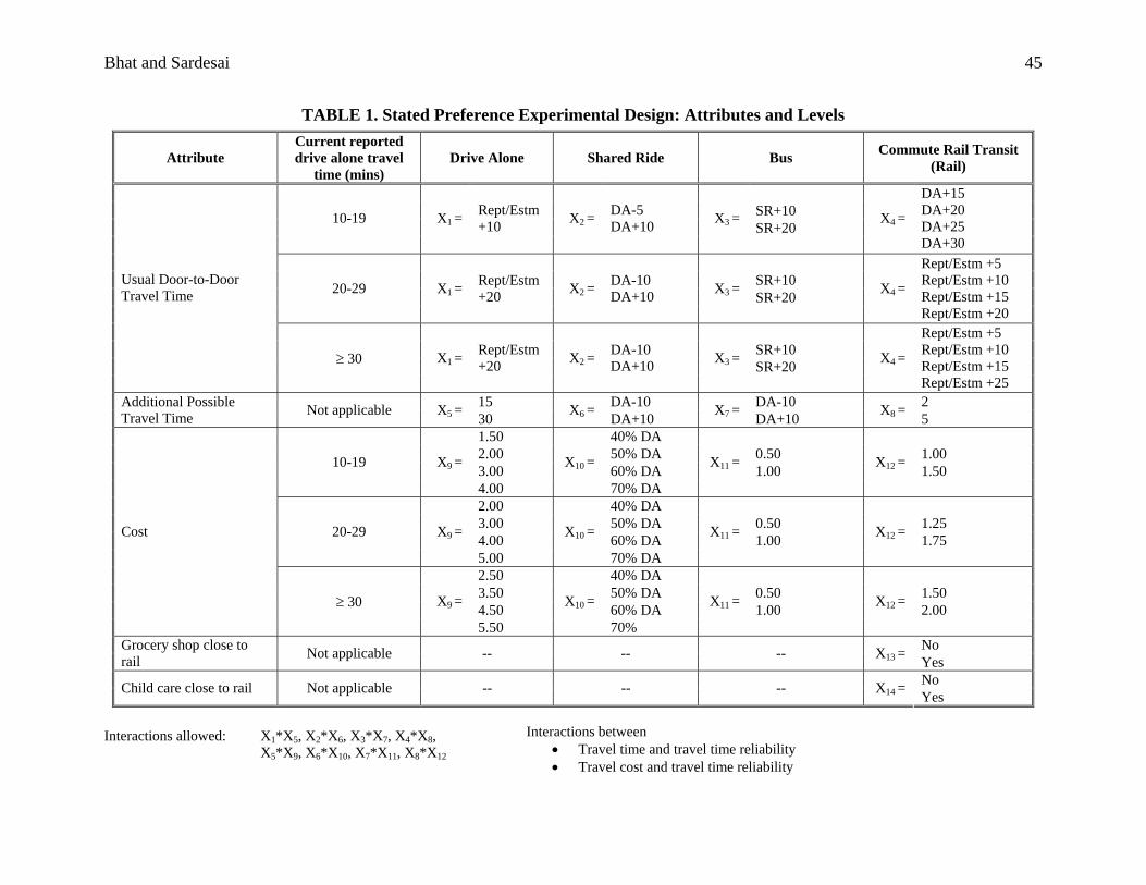
Bhat and Sardesai 45
TABLE 1. Stated Preference Experimental Design: Attributes and Levels
Interactions allowed: X1*X5, X2*X6, X3*X7, X4*X8,
X5*X9, X6*X10, X7*X11, X8*X12
Attribute Current reported drive alone travel
time (mins) Drive Alone Shared Ride Bus Commute Rail Transit
(Rail)
SR+10 SR+20
10-19 X1 =Rept/Estm +10 X2 =
DA-5 DA+10 X3 =
X4 =
DA+15 DA+20 DA+25 DA+30
SR+10 SR+20 20-29 X1 =
Rept/Estm +20 X2 =
DA-10 DA+10 X3 =
X4 =
Rept/Estm +5 Rept/Estm +10 Rept/Estm +15 Rept/Estm +20
SR+10 SR+20
Usual Door-to-Door Travel Time
≥ 30 X1 =Rept/Estm +20 X2 =
DA-10 DA+10 X3
X4 =
Rept/Estm +5 Rept/Estm +10 Rept/Estm +15 Rept/Estm +25
15 DA-10 DA-10 2 Additional Possible Travel Time Not applicable X5 = 30 X6 = DA+10 X7 DA+10 X8 = 5
1.50 40% DA2.00 50% DA 0.50 1.003.00 60% DA 1.00 1.5010-19 X9 =
4.00
X10 =
70% DA
X11
X12 =
2.00 40% DA3.00 50% DA 0.50 1.254.00 60% DA 1.00 1.7520-29 X9 =
5.00
X10 =
70% DA
X11
X12 =
2.50 40% DA3.50 50% DA 0.50 1.504.50 60% DA 1.00 2.00
Cost
≥ 30 X9 =
5.50
X10 =
70%
X11 X12 =
Grocery shop close to rail Not applicable -- --
Child care close to rail Not applicable -- --
Interactions between • Travel time and travel time• Travel cost and travel time
=
=
=
=
=
No -- X13 = Yes No -- X14 = Yes
reliability reliability

Revealed Preference Sample Stated Preference Sample Joint Sample Alternative
Availability percentages 1
Choice percentages
Availability percentages 1
Choice percentages
Availability percentages 1
Choice percentages
Drive alone 98.5 86.1 99.4 45.2 99.1 59.5
Shared ride 100.0 7.5 100.0 13.8 100.0 11.6
Bus 42.9 3.4 100.0 5.7 80.2 4.9
Non-motorized mode 20.8 3.0 -- -- 7.2 23.0
Commuter Rail Transit (Rail) -- -- 100.0 35.3 65.3 1.0
Sample Size 679 1276 1955
46
TABLE 2. Availability and Choice Percentages of Alternatives
1 The availability percentages represent the percentage of observations in the sample for which the alternative is available.
Bhat and Sardesai
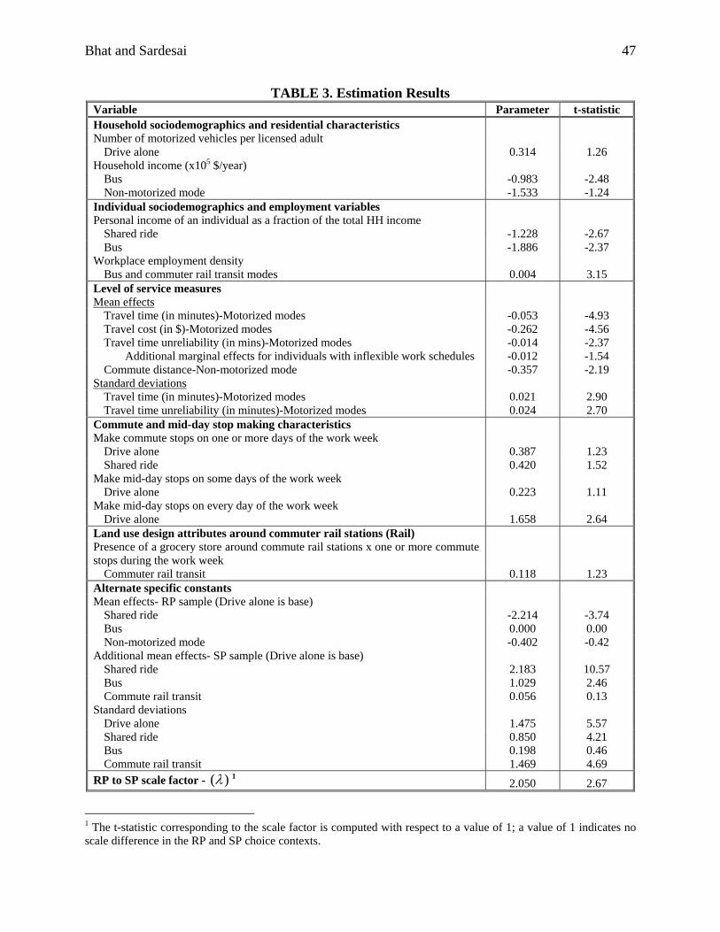
Bhat and Sardesai 47
TABLE 3. Estimation Results Variable Parameter t-statistic Household sociodemographics and residential characteristics Number of motorized vehicles per licensed adult
Drive alone 0.314 1.26 Household income (x105 $/year)
Bus -0.983 -2.48 Non-motorized mode -1.533 -1.24
Individual sociodemographics and employment variables Personal income of an individual as a fraction of the total HH income
Shared ride -1.228 -2.67 Bus -1.886 -2.37
Workplace employment density Bus and commuter rail transit modes 0.004 3.15
Level of service measures Mean effects
Travel time (in minutes)-Motorized modes -0.053 -4.93 Travel cost (in $)-Motorized modes -0.262 -4.56 Travel time unreliability (in mins)-Motorized modes -0.014 -2.37
Additional marginal effects for individuals with inflexible work schedules -0.012 -1.54 Commute distance-Non-motorized mode -0.357 -2.19
Standard deviations Travel time (in minutes)-Motorized modes 0.021 2.90 Travel time unreliability (in minutes)-Motorized modes 0.024 2.70
Commute and mid-day stop making characteristics Make commute stops on one or more days of the work week
Drive alone 0.387 1.23 Shared ride 0.420 1.52
Make mid-day stops on some days of the work week Drive alone 0.223 1.11
Make mid-day stops on every day of the work week Drive alone 1.658 2.64
Land use design attributes around commuter rail stations (Rail) Presence of a grocery store around commute rail stations x one or more commute stops during the work week
Commuter rail transit 0.118 1.23 Alternate specific constants Mean effects- RP sample (Drive alone is base)
Shared ride -2.214 -3.74 Bus 0.000 0.00 Non-motorized mode -0.402 -0.42
Additional mean effects- SP sample (Drive alone is base) Shared ride 2.183 10.57 Bus 1.029 2.46 Commute rail transit 0.056 0.13
Standard deviations Drive alone 1.475 5.57 Shared ride 0.850 4.21 Bus 0.198 0.46 Commute rail transit 1.469 4.69
RP to SP scale factor - ( )λ 12.050 2.67
1 The t-statistic corresponding to the scale factor is computed with respect to a value of 1; a value of 1 indicates no scale difference in the RP and SP choice contexts.
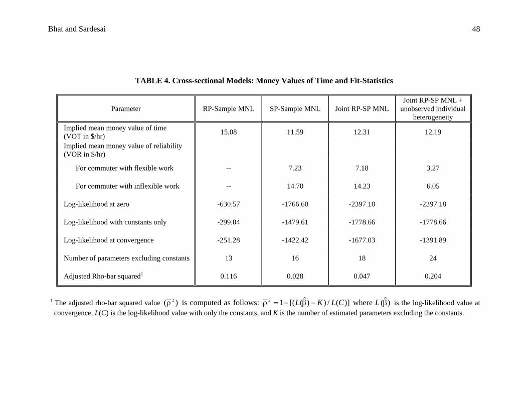
Bhat and Sardesai 48
TABLE 4. Cross-sectional Models: Money Values of Time and Fit-Statistics
Parameter RP-Sample MNL SP-Sample MNL Joint RP-SP MNL Joint RP-SP MNL +
unobserved individual heterogeneity
Implied mean money value of time (VOT in $/hr) 15.08 11.59 12.31 12.19
Implied mean money value of reliability (VOR in $/hr)
For commuter with flexible work -- 7.23 7.18 3.27
For commuter with inflexible work -- 14.70 14.23 6.05
Log-likelihood at zero -630.57 -1766.60 -2397.18 -2397.18
Log-likelihood with constants only -299.04 -1479.61 -1778.66 -1778.66
Log-likelihood at convergence -251.28 -1422.42 -1677.03 -1391.89
Number of parameters excluding constants 13 16 18 24
Adjusted Rho-bar squared1 0.116 0.028 0.047 0.204
1 The adjusted rho-bar squared value )( 2ρ is computed as follows: )](/))ˆ([(12 CLKL −β−=ρ where L is the log-likelihood value at
convergence, L(C) is the log-likelihood value with only the constants, and K is the number of estimated parameters excluding the constants. )ˆ(β
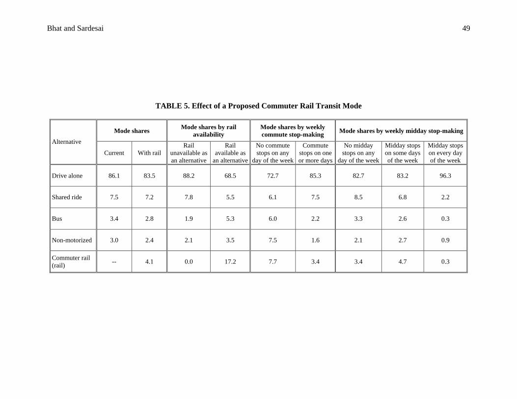
Bhat and Sardesai 49
TABLE 5. Effect of a Proposed Commuter Rail Transit Mode
Mode shares Mode shares by rail availability
Mode shares by weekly commute stop-making Mode shares by weekly midday stop-making
Alternative
Current With railRail
unavailable as an alternative
Rail available as
an alternative
No commute stops on any
day of the week
Commute stops on one or more days
No midday stops on any
day of the week
Midday stops on some days of the week
Midday stops on every day of the week
Drive alone 86.1 83.5 88.2 68.5 72.7 85.3 82.7 83.2 96.3
Shared ride 7.5 7.2 7.8 5.5 6.1 7.5 8.5 6.8 2.2
Bus 3.4 2.8 1.9 5.3 6.0 2.2 3.3 2.6 0.3
Non-motorized 3.0 2.4 2.1 3.5 7.5 1.6 2.1 2.7 0.9
Commuter rail (rail) -- 4.1 0.0 17.2 7.7 3.4 3.4 4.7 0.3

Bhat and Sardesai 50
TABLE 6. Effect of Tolls on Travel Mode Shares
No toll case $1.00 toll $2.00 toll Alternative
Overall Highway users
Non-highway users Overall Highway
users Non-highway
users Overall Highway users
Non-highway users
Drive alone 83.5 87.5 77.5 82.0 85.1 77.5 80.3 82.3 77.5
Shared ride 7.2 7.5 6.8 8.2 9.1 6.8 9.2 10.9 6.8
Bus 2.8 1.8 4.2 2.9 2.1 4.2 3.2 2.5 4.2
Non-motorized 2.4 1.4 4.0 2.6 1.7 4.0 2.9 2.0 4.0
Commuter rail (rail) 4.1 1.8 7.5 4.3 2.0 7.5 4.4 2.3 7.5