Measuring Travel TimeMeasuring Travel Time Reliability in the Miami Valley

Technical Advisory CommitteeDayton, OHy ,September 16, 2010

A dAgenda

O er ie of FMS Data Overview of FMS Data Definitions Travel Time Analysis Average Speed Mapsg p p Corridor Ranking Comparison with Other Regions Comparison with Other Regions Future Steps

PPurpose

Tra el Time reliabilit is the consistenc or Travel Time reliability is the consistency or dependability in travel times, as measured from day to day and/or across different times of the dayday and/or across different times of the day.

Measures of Travel Time Reliability: Are important indicators of the health of a

transportation system; Can reveal changes in system conditions from year to

year; Can supplement existing congestion measures such as

v/c ratios, vehicle hours of delay, and mean speed.

Mi i V ll T l Ti DMiami Valley Travel Time Data

ODOT provided data CLARKMIAMI ODOT provided data

from the Intelligent Transportation pSystem sensors for 36 corridor segments

Data initially provided in MS Excel

d h t d l tspreadsheets and later MS Access databases GREENE

0 1 2 3Miles

MONTGOMERY

WARREN

FMS D ( d )FMS Data (contd.)

Continuous raw data provided recorded travel time for Continuous raw data provided recorded travel time for approximately every minute for each travel segment resulting in nearly a million records of data for each monthy

FMS Data (contd )FMS Data (contd.) The raw data was checked for estimation errors It was then summarized to produce hourly average travel

times for each segment for each day of each month of the year

Several statistics were calculated for each segment from gthis condensed data: Average Travel Time by Hour and Weekday 95th percentile Travel Time by Hour and Weekday Free Flow Travel Time Indices including Buffer Time Index, Travel Time Index

and Planning Time Index.

D fi i iDefinitions

95th Percentile Travel Time: ho m ch dela ill be 95th Percentile Travel Time: how much delay will be on the heaviest travel days

l i h h i Free Flow Travel Time: travel time when there is no congestion delay

Travel Time Index: average time it takes to travel during peak hours compared to free flow conditions

Buffer Index: extra time so one is on time most of the time

Planning Time Index: total time needed to plan for an on-time arrival 95% of the timeon time arrival 95% of the time

Travel Time Analysis: I-70Travel Time Analysis: I-70

Free Flow Travel Time Average Travel Time 95th Percentile Travel Time

Travel Time Analysis: I-75Travel Time Analysis: I-75

Free Flow Travel Time Average Travel Time 95th Percentile Travel Time

Travel Time Analysis: US 35Travel Time Analysis: US 35

Corridor RankingsFree Flow Travel Time Average Travel Time 95th Percentile Travel Time

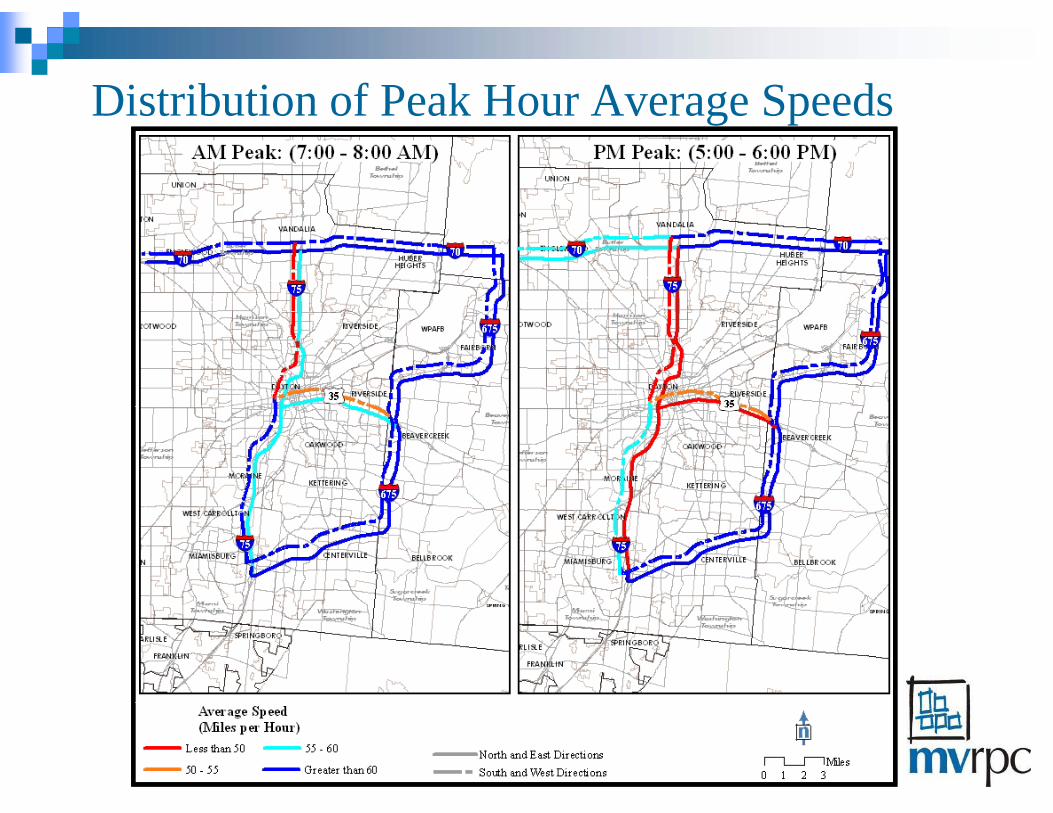
Distribution of Peak Hour Average SpeedsDistribution of Peak Hour Average Speeds

A S d Di ib i bAverage Speed Distributions by:Time of Day

Month Weekday

Mi I dMisery Index Seeks to measure the length of delay of only the worst Seeks to measure the length of delay of only the worst

trips It is computed according to the following formula: It is computed according to the following formula:

Corridors Misery IndexI-75: Between US 35 and I-70 0.43

I-75: Between I-675 and US 35 0.34

I 70 B t SR49 d I 75 0 26I-70: Between SR49 and I-75 0.26

I-70: Between I-75 and I-675 0.32

US 35: Between I-75 and I-675 0.29

C i C i I diComparative Congestion IndicesCity Congested Hours Travel Time Index Planning Time Index

Chicago, IL 9:39 1.39 1.74Chicago, IL 9:39 1.39 1.74Los Angeles, CA 6:28 1.29 1.59Seattle, WA 5:22 1.29 1.72Philadelphia, PA 6:14 1.28 1.66B t MA 5 26 1 27 1 63Boston, MA 5:26 1.27 1.63Houston, TX 3:31 1.24 1.51Portland, OR 1:39 1.23 1.62Atlanta, GA 4:13 1.22 1.58Detroit, MI 3:20 1.2 1.5Pittsburgh, PA 7:53 1.2 1.43Minneapolis-St. Paul, MN 4:18 1.19 1.48Orange County, CA 3:34 1.19 1.46g y,Dayton, OH (I-75 SB PM Peak Hour) 2:00 1.15 1.5San Francisco, CA 2:53 1.13 1.32Riverside – San Bernardino, CA 2:58 1.1 1.25St Louis MO 1:44 1 1 1 27St. Louis, MO 1:44 1.1 1.27San Diego, CA 2:14 1.1 1.29Providence, RI 2:14 1.08 1.24Sacramento, CA 1:55 1.08 1.21Tampa, FL 2:21 1.08 1.21Oklahoma City, OK 1:37 1.06 1.19Salt Lake City, UT 3:15 1.05 1.16

C l iConclusions

I 75 N corridor bet een US 35 and I 70 is the most I-75 N corridor between US 35 and I-70 is the most congested freeway corridor in the Miami Valley while I 70 E from I 75 to I 675 is the least congestedI-70 E from I-75 to I-675 is the least congested.

Average speeds remain close to the set speed limits on ll id h id d i kall corridors except the I-75 corridor during peak

hours. No discernable variation exists between different

months, but the average speeds tend to be lower on weekdays and much higher on weekends except in certain construction zones.

ChallengesChallenges Data Intensive Exercise: continuous supply of error-

f d t i dfree data required Hardware Capability: need appropriate computer

hardware to process and store large amounts of data Software Capability: need software applications that p y pp

can handle large databases and process results fairly quicklyq y

F SFuture Steps

Contin e pdating database ith ne data from Continue updating database with new data from ODOT

h l hl d l i Do hourly, monthly and annual comparisons to determine travel time reliability

Determine project impacts on travel times by comparing pre- and post construction data

Document findings in the Congestion Management Process Report updates.p p

Questions and Answers