The impact of permafrost degradation on methane...

i

Student thesis series INES nr 372

Andreas Dahlbom

The impact of permafrost degradation on methane fluxes - a field study in Abisko

2016

Department of

Physical Geography and Ecosystem Science

Lund University

Sölvegatan 12

S-223 62 Lund

Sweden

ii

Andreas Dahlbom (2016).

The impact of permafrost degradation on methane fluxes - a field study in Abisko.

Master degree thesis, 30 credits in Physical Geography and Ecosystem Analysis

Department of Physical Geography and Ecosystem Science, Lund University

Level: Master of Science (MSc)

Course duration: August 2015 until January 2016

Disclaimer

This document describes work undertaken as part of a program of study at the University

of Lund. All views and opinions expressed herein remain the sole responsibility of the

author, and do not necessarily represent those of the institute.

iii

The impact of permafrost degradation on methane fluxes

- a field study in Abisko

Andreas Dahlbom

Master thesis, 30 credits, in

Physical Geography and Ecosystem Analysis

Torben Christensen

Dept. of Physical Geography and Ecosystems Science

Marcin Jackowicz-Korczynski


Mikhail Mastepanov


Exam committee:

Thomas Holst


Lena Ström


http://www.lunduniversity.lu.se/lucat/group/v1000639





iv

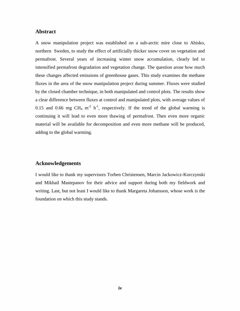
Abstract

A snow manipulation project was established on a sub-arctic mire close to Abisko,

northern Sweden, to study the effect of artificially thicker snow cover on vegetation and

permafrost. Several years of increasing winter snow accumulation, clearly led to

intensified permafrost degradation and vegetation change. The question arose how much

these changes affected emissions of greenhouse gases. This study examines the methane

fluxes in the area of the snow manipulation project during summer. Fluxes were studied

by the closed chamber technique, in both manipulated and control plots. The results show

a clear difference between fluxes at control and manipulated plots, with average values of

0.15 and 0.66 mg CH4 m-2

h-1

, respectively. If the trend of the global warming is

continuing it will lead to even more thawing of permafrost. Then even more organic

material will be available for decomposition and even more methane will be produced,

adding to the global warming.

Acknowledgements

I would like to thank my supervisors Torben Christensen, Marcin Jackowicz-Korczynski

and Mikhail Mastepanov for their advice and support during both my fieldwork and

writing. Last, but not least I would like to thank Margareta Johansson, whose work is the

foundation on which this study stands.

v

Table of content

INTRODUCTION............................................................................................................. 1

Methane ......................................................................................................................................................... 1

Permafrost ..................................................................................................................................................... 2

Permafrost dynamics at climate change ..................................................................................................... 3

Aims ............................................................................................................................................................... 5

METHODS AND MATERIALS ..................................................................................... 6

Site description ............................................................................................................................................. 6

Experimental setup ....................................................................................................................................... 8

Chamber measurements .............................................................................................................................. 9

Other variables ............................................................................................................................................11

RESULTS ........................................................................................................................ 13

DISCUSSION .................................................................................................................. 22

Permafrost ....................................................................................................................................................22

Equipment ....................................................................................................................................................22

Methane ........................................................................................................................................................23

Vascular plants ............................................................................................................................................25

CONCLUSIONS ............................................................................................................. 27

REFERENCES ................................................................................................................ 28

1

Introduction

Methane

Methane (CH4) is a greenhouse gas that is produced when biomass is decomposed under

anaerobic conditions (without oxygen) (AMAP 2012). The amount of methane in the

atmosphere in comparison to carbon dioxide (CO2) is small. Even though the emissions

of CH4 are smaller than CO2, it is one of the most important contributor to the global

warming (Jackowicz-Korczyński et al. 2010; AMAP 2012). This is because CH4 is over

25 times more potent as a greenhouse gas than CO2 over a 100 year time span (IPCC

2014). In 2014 the global average concentrations of CH4 in the atmosphere was 1833±1

ppb (parts per billion) and for CO2 it was 397.7±0.1ppm (parts per million)(WMO 2015).

Since the start of the industrial revolution, the amount of CH4 has more than doubled.

During the same time the amount of CO2 has risen around only 30% (Norina 2007). CH4

is not as long lived in the atmosphere as CO2, only around 9 years in comparison to 34-44

years (Seinfeld and Pandis 2006), but long lived enough to have an impact on a global

scale. From 2013 to 2014 the global average concentration of CH4 increased by 9 ppb,

and during the same period CO2 increased 1,9ppm (WMO 2015).

Figure 1: A conceptual flow chart of the CH4 pathway. In areas where permafrost is present this takes place

in the active layer. Taken from (Whalen 2005).

2

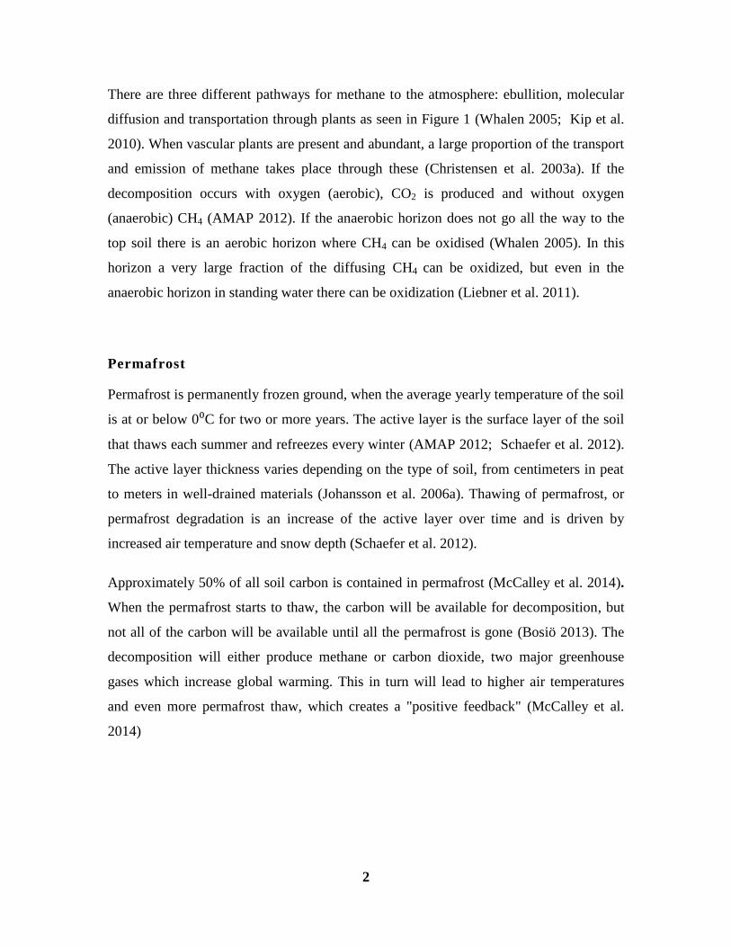
There are three different pathways for methane to the atmosphere: ebullition, molecular

diffusion and transportation through plants as seen in Figure 1 (Whalen 2005; Kip et al.

2010). When vascular plants are present and abundant, a large proportion of the transport

and emission of methane takes place through these (Christensen et al. 2003a). If the

decomposition occurs with oxygen (aerobic), CO2 is produced and without oxygen

(anaerobic) CH4 (AMAP 2012). If the anaerobic horizon does not go all the way to the

top soil there is an aerobic horizon where CH4 can be oxidised (Whalen 2005). In this

horizon a very large fraction of the diffusing CH4 can be oxidized, but even in the

anaerobic horizon in standing water there can be oxidization (Liebner et al. 2011).

Permafrost

Permafrost is permanently frozen ground, when the average yearly temperature of the soil

is at or below 0⁰C for two or more years. The active layer is the surface layer of the soil

that thaws each summer and refreezes every winter (AMAP 2012; Schaefer et al. 2012).

The active layer thickness varies depending on the type of soil, from centimeters in peat

to meters in well-drained materials (Johansson et al. 2006a). Thawing of permafrost, or

permafrost degradation is an increase of the active layer over time and is driven by

increased air temperature and snow depth (Schaefer et al. 2012).

Approximately 50% of all soil carbon is contained in permafrost (McCalley et al. 2014).

When the permafrost starts to thaw, the carbon will be available for decomposition, but

not all of the carbon will be available until all the permafrost is gone (Bosiö 2013). The

decomposition will either produce methane or carbon dioxide, two major greenhouse

gases which increase global warming. This in turn will lead to higher air temperatures

and even more permafrost thaw, which creates a "positive feedback" (McCalley et al.

2014)

3

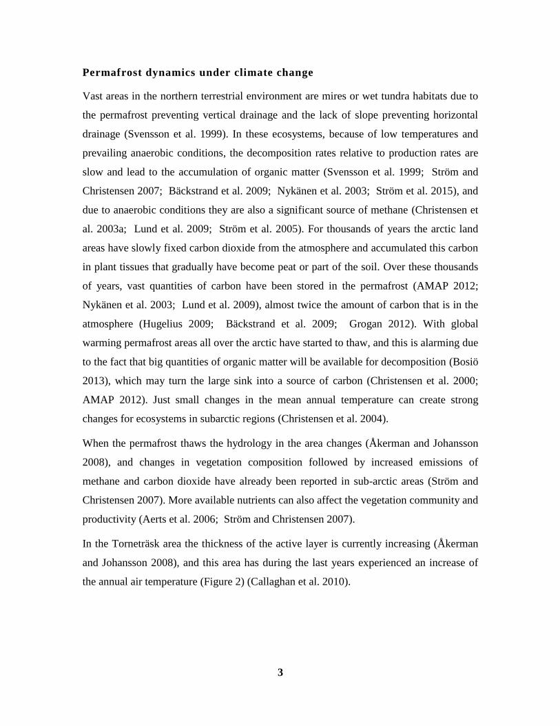
Permafrost dynamics under climate change

Vast areas in the northern terrestrial environment are mires or wet tundra habitats due to

the permafrost preventing vertical drainage and the lack of slope preventing horizontal

drainage (Svensson et al. 1999). In these ecosystems, because of low temperatures and

prevailing anaerobic conditions, the decomposition rates relative to production rates are

slow and lead to the accumulation of organic matter (Svensson et al. 1999; Ström and

Christensen 2007; Bäckstrand et al. 2009; Nykänen et al. 2003; Ström et al. 2015), and

due to anaerobic conditions they are also a significant source of methane (Christensen et

al. 2003a; Lund et al. 2009; Ström et al. 2005). For thousands of years the arctic land

areas have slowly fixed carbon dioxide from the atmosphere and accumulated this carbon

in plant tissues that gradually have become peat or part of the soil. Over these thousands

of years, vast quantities of carbon have been stored in the permafrost (AMAP 2012;

Nykänen et al. 2003; Lund et al. 2009), almost twice the amount of carbon that is in the

atmosphere (Hugelius 2009; Bäckstrand et al. 2009; Grogan 2012). With global

warming permafrost areas all over the arctic have started to thaw, and this is alarming due

to the fact that big quantities of organic matter will be available for decomposition (Bosiö

2013), which may turn the large sink into a source of carbon (Christensen et al. 2000;

AMAP 2012). Just small changes in the mean annual temperature can create strong

changes for ecosystems in subarctic regions (Christensen et al. 2004).

When the permafrost thaws the hydrology in the area changes (Åkerman and Johansson

2008), and changes in vegetation composition followed by increased emissions of

methane and carbon dioxide have already been reported in sub-arctic areas (Ström and

Christensen 2007). More available nutrients can also affect the vegetation community and

productivity (Aerts et al. 2006; Ström and Christensen 2007).

In the Torneträsk area the thickness of the active layer is currently increasing (Åkerman

and Johansson 2008), and this area has during the last years experienced an increase of

the annual air temperature (Figure 2) (Callaghan et al. 2010).

4

Figure 2: This Figure is taken from (Callaghan et al. 2010) and it shows the annual air temperature for the

Abisko region for the last 100 years and the vertical line before 1995 shows where the annual temperature

starts to rise above 0⁰C. The red line is a polynomial curve trough the local maxima, the blue through the

local minima and the black is a smoothed mean annual air temperature.

In high latitudes, ecosystem functions and vegetation are greatly affected by snow. For

example in cold regions where the growing season is short, a few weeks change in season

length can have a great impact (Høye et al. 2007). This can also affect the hydrology and

ecological systems (Callaghan et al. 2011). Climate scenarios for the Abisko region

predict an increase of ≈2% of precipitation per decade over the coming 60 years, and the

predicted precipitation is expected to be higher during winter than summer (Sælthun and

Barkved 2003). A explanation for this is that higher surface temperature over the northern

Atlantic causes higher evaporation and then increased precipitation over the Lapland

region (Seppälä 2003). The majority of the projected precipitation for the Abisko area

will be in autumn and winter (Sælthun and Barkved 2003), which will lead to increased

snow fall and snow depth. Changes in snow cover have already been observed and

evidence in the form of thawing permafrost, increases in active layer and vegetation

changes have been reported during the last decade (Åkerman and Johansson 2008). With

increased snow depth there is also an increased water source in the spring when the snow

melts, which can lead to a higher water table (Bosiö et al. 2014).

As a rough generalization, permafrost can be formed and sustained in areas with an

annual mean air temperature of 0⁰C or less, but when the temperature increases, the

permafrost starts to thaw. When snow covers areas with permafrost during the winter, the

snow acts like a blanket and slows the heat loss of the ground. When the heat loss during

the winter is less than heat gain during summer, the active layer increases every year until

there is no more permafrost.

5

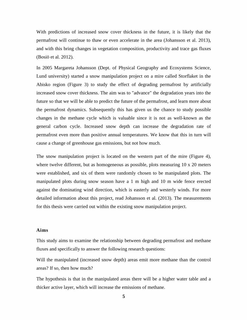
With predictions of increased snow cover thickness in the future, it is likely that the

permafrost will continue to thaw or even accelerate in the area (Johansson et al. 2013),

and with this bring changes in vegetation composition, productivity and trace gas fluxes

(Bosiö et al. 2012).

In 2005 Margareta Johansson (Dept. of Physical Geography and Ecosystems Science,

Lund university) started a snow manipulation project on a mire called Storflaket in the

Abisko region (Figure 3) to study the effect of degrading permafrost by artificially

increased snow cover thickness. The aim was to "advance" the degradation years into the

future so that we will be able to predict the future of the permafrost, and learn more about

the permafrost dynamics. Subsequently this has given us the chance to study possible

changes in the methane cycle which is valuable since it is not as well-known as the

general carbon cycle. Increased snow depth can increase the degradation rate of

permafrost even more than positive annual temperatures. We know that this in turn will

cause a change of greenhouse gas emissions, but not how much.

The snow manipulation project is located on the western part of the mire (Figure 4),

where twelve different, but as homogeneous as possible, plots measuring 10 x 20 meters

were established, and six of them were randomly chosen to be manipulated plots. The

manipulated plots during snow season have a 1 m high and 10 m wide fence erected

against the dominating wind direction, which is easterly and westerly winds. For more

detailed information about this project, read Johansson et al. (2013). The measurements

for this thesis were carried out within the existing snow manipulation project.

Aims

This study aims to examine the relationship between degrading permafrost and methane

fluxes and specifically to answer the following research questions:

Will the manipulated (increased snow depth) areas emit more methane than the control

areas? If so, then how much?

The hypothesis is that in the manipulated areas there will be a higher water table and a

thicker active layer, which will increase the emissions of methane.


6

The growing season in the manipulated areas is shortened due to the artificially increased

snow depth. With the assumed higher emission rate of methane, will the manipulated

areas emit more methane over the whole season in comparison to the control areas?

The hypothesis is that there will be more accumulative emissions from the manipulated

plots in comparison to control, due to higher fluxes of methane from manipulated plots

and a long growing season in total.

Methods and materials

As a result of climate change, arctic and sub-arctic peatlands are expected to emit higher

amounts of methane. This study was conducted at the sub-arctic mire Storflaket, close to

Abisko, Northern Sweden. CH4 fluxes were measured in an area where a snow

manipulation project has influenced the permafrost. Because it was not known whether or

not CH4 concentrations during measurements would show a clear trend, CO2 was also

measured simultaneously as a quality check on the measurements of CH4. CO2

measurements can be used as such because under dark chamber conditions only a steady

rise in CO2 concentrations can be expected (due to no photosynthesis and only respiration

taking place).

Site description

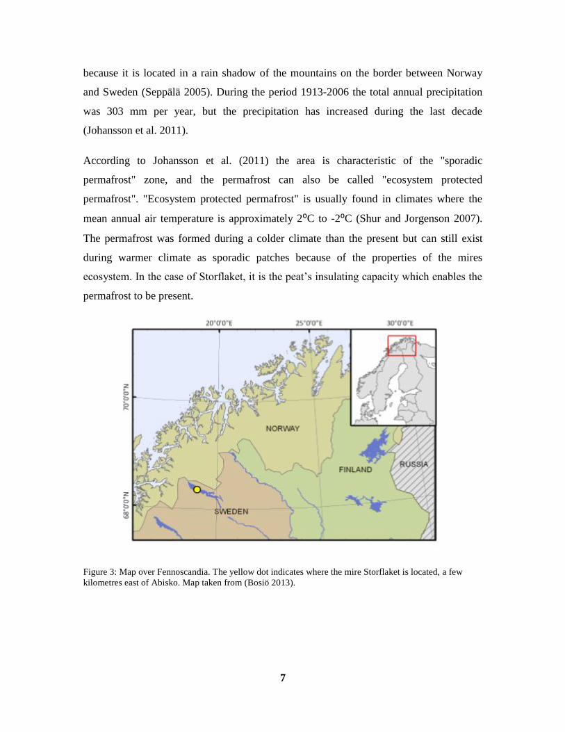
CO2 and CH4 fluxes were measured on a mire called Storflaket, which is located in the

northernmost Sweden (Figure 3), 6 km East of the Abisko scientific research station

(68°20'47.60''N 18°58'22.10''E). The mire is approximately 13 ha and has a 60-90 cm

thick peat layer and the plant community is classified as tundra because of the underlying

permafrost (Bosiö et al. 2014). The road E10 between Kiruna and Narvik borders the

mire to the north, a railway to the south and a birch forest to the east and the west

(Johansson et al. 2013). The Abisko region has relatively low amounts of precipitation

7

because it is located in a rain shadow of the mountains on the border between Norway

and Sweden (Seppälä 2005). During the period 1913-2006 the total annual precipitation

was 303 mm per year, but the precipitation has increased during the last decade

(Johansson et al. 2011).

According to Johansson et al. (2011) the area is characteristic of the "sporadic

permafrost" zone, and the permafrost can also be called "ecosystem protected

permafrost". "Ecosystem protected permafrost" is usually found in climates where the

mean annual air temperature is approximately 2⁰C to -2⁰C (Shur and Jorgenson 2007).

The permafrost was formed during a colder climate than the present but can still exist

during warmer climate as sporadic patches because of the properties of the mires

ecosystem. In the case of Storflaket, it is the peat’s insulating capacity which enables the

permafrost to be present.

Figure 3: Map over Fennoscandia. The yellow dot indicates where the mire Storflaket is located, a few

kilometres east of Abisko. Map taken from (Bosiö 2013).

8

Experimental setup

Figure 4: Aerial view of the placement of the plots at the mire Storflaket. The green dots are the control

plots and the white ones are the manipulated plots. The satellite photo is from Google Earth and is retrieved

on the 25th of August 2014.

By eye it was clear to see that the western side of the manipulated plots was more

affected than the eastern side (more degraded). It was therefore decided to take the

majority of the CH4 and CO2 measurements on the western side of all plots (both in

control and manipulated plots).

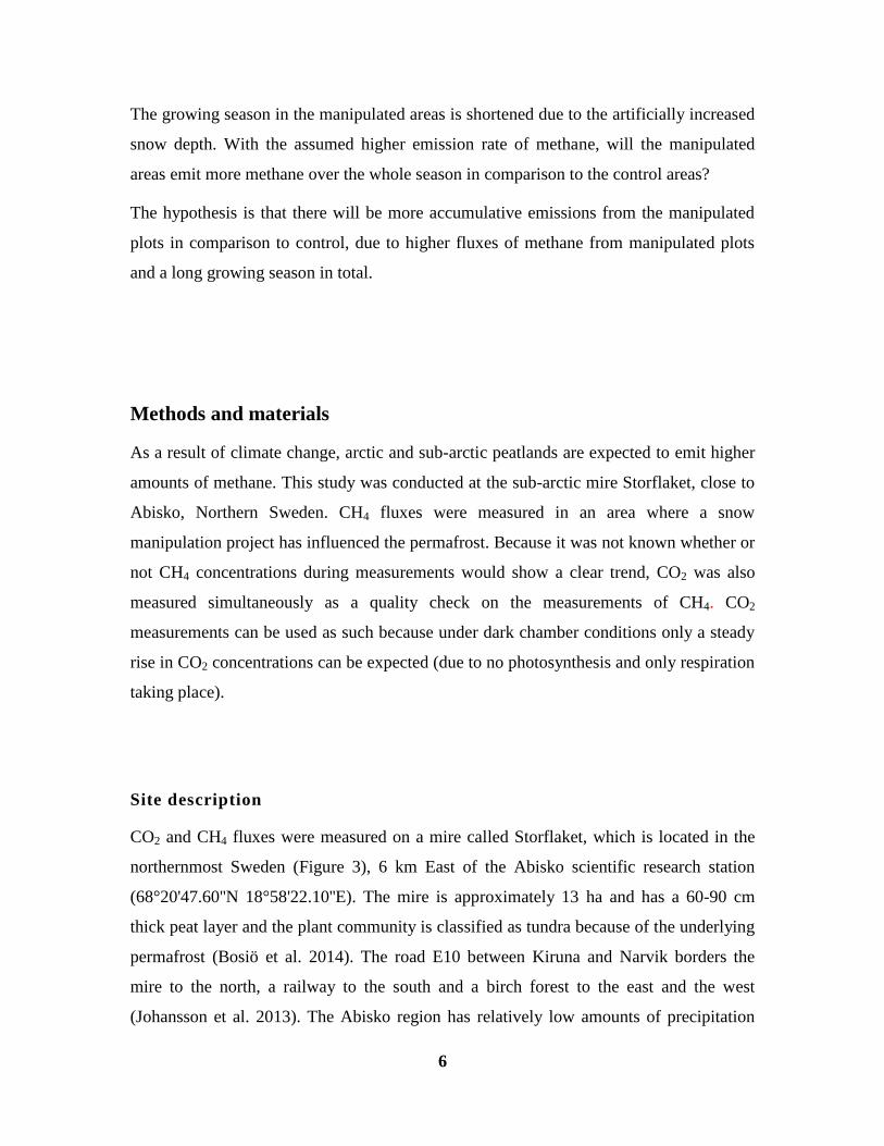
Of the twelve plots, it measurements were taken in a total of six subplots. Subplots one to

five were put out according to a grid (Figure 5) that was determined prior to the

measurements, and subplot number six was put on one already installed collar on the east

side of the snow fence (Figure 5). Because of the subplots’ vegetation and tilt the

placement of the chamber was in a radius of one meter from the original placement to

find an as levelled area as possible to make the chambers as airtight as possible.

9

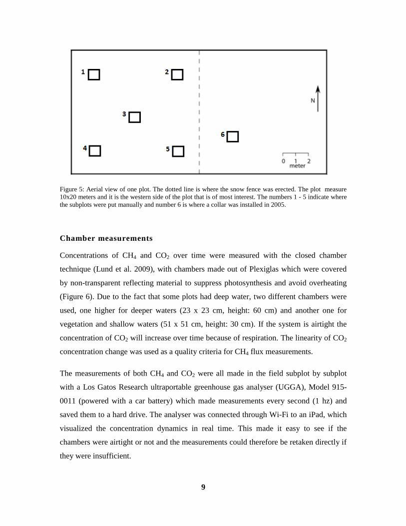
Figure 5: Aerial view of one plot. The dotted line is where the snow fence was erected. The plot measure

10x20 meters and it is the western side of the plot that is of most interest. The numbers 1 - 5 indicate where

the subplots were put manually and number 6 is where a collar was installed in 2005.

Chamber measurements

Concentrations of CH4 and CO2 over time were measured with the closed chamber

technique (Lund et al. 2009), with chambers made out of Plexiglas which were covered

by non-transparent reflecting material to suppress photosynthesis and avoid overheating

(Figure 6). Due to the fact that some plots had deep water, two different chambers were

used, one higher for deeper waters (23 x 23 cm, height: 60 cm) and another one for

vegetation and shallow waters (51 x 51 cm, height: 30 cm). If the system is airtight the

concentration of CO2 will increase over time because of respiration. The linearity of CO2

concentration change was used as a quality criteria for CH4 flux measurements.

The measurements of both CH4 and CO2 were all made in the field subplot by subplot

with a Los Gatos Research ultraportable greenhouse gas analyser (UGGA), Model 915-

0011 (powered with a car battery) which made measurements every second (1 hz) and

saved them to a hard drive. The analyser was connected through Wi-Fi to an iPad, which

visualized the concentration dynamics in real time. This made it easy to see if the

chambers were airtight or not and the measurements could therefore be retaken directly if

they were insufficient.

10

Inside of the chambers a thermometer was

attached and a fan was put in to circulate the air.

From the chamber two plastic tubes with a length

of 40 meters and an inner diameter of 4 mm were

connected to the ultraportable gas analyser for the

gas content in the chamber to circulate through

the machine.

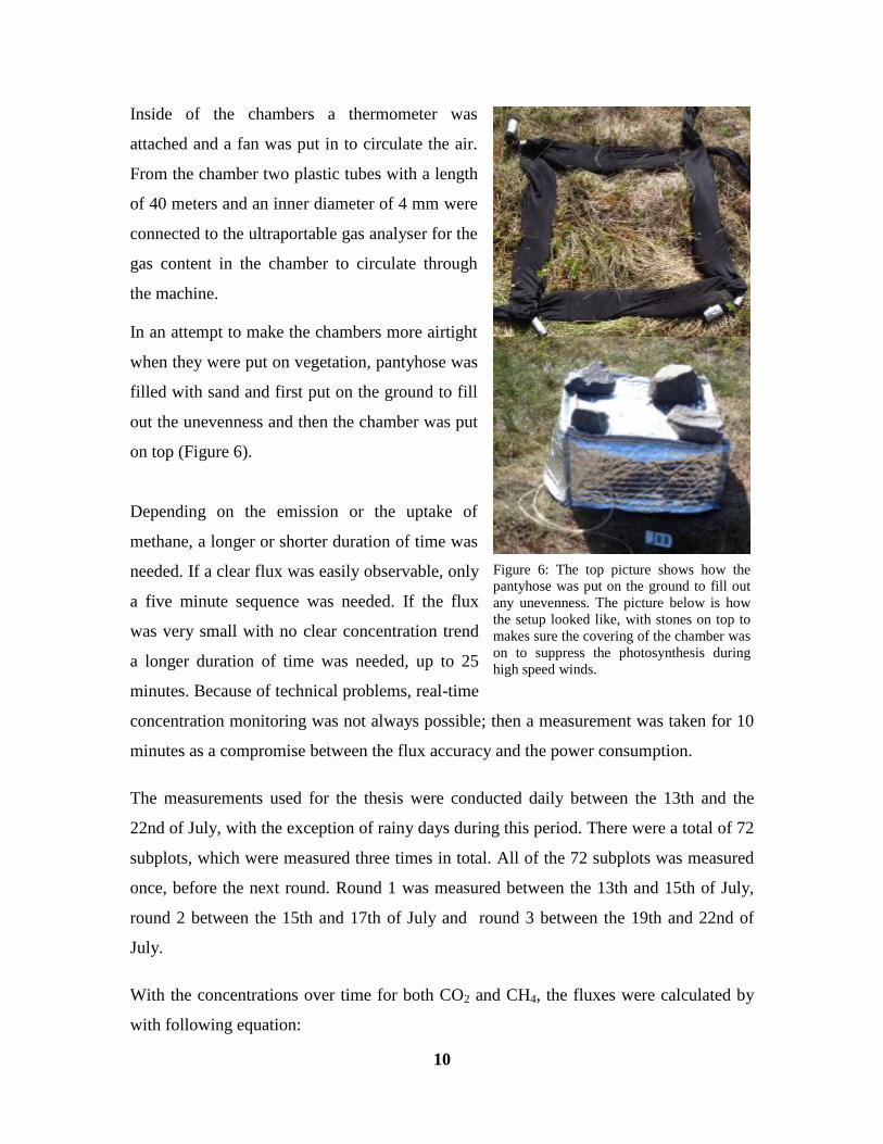
In an attempt to make the chambers more airtight

when they were put on vegetation, pantyhose was

filled with sand and first put on the ground to fill

out the unevenness and then the chamber was put

on top (Figure 6).

Depending on the emission or the uptake of

methane, a longer or shorter duration of time was

needed. If a clear flux was easily observable, only

a five minute sequence was needed. If the flux

was very small with no clear concentration trend

a longer duration of time was needed, up to 25

minutes. Because of technical problems, real-time

concentration monitoring was not always possible; then a measurement was taken for 10

minutes as a compromise between the flux accuracy and the power consumption.

The measurements used for the thesis were conducted daily between the 13th and the

22nd of July, with the exception of rainy days during this period. There were a total of 72

subplots, which were measured three times in total. All of the 72 subplots was measured

once, before the next round. Round 1 was measured between the 13th and 15th of July,

round 2 between the 15th and 17th of July and round 3 between the 19th and 22nd of

July.

With the concentrations over time for both CO2 and CH4, the fluxes were calculated by

with following equation:

Figure 6: The top picture shows how the

pantyhose was put on the ground to fill out

any unevenness. The picture below is how

the setup looked like, with stones on top to

makes sure the covering of the chamber was

on to suppress the photosynthesis during

high speed winds.

11

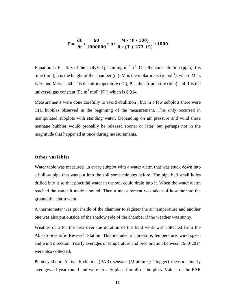
Equation 1: F = flux of the analyzed gas in mg m-2

h-1

. C is the concentration (ppm), t is

time (min), h is the height of the chamber (m). M is the molar mass (g mol-1

), where MCH4

is 16 and MCO2 is 44. T is the air temperature (⁰C), P is the air pressure (hPa) and R is the

universal gas constant (Pa m3 mol

-1 K

-1) which is 8.314.

Measurements were done carefully to avoid ebullition , but in a few subplots there were

CH4 bubbles observed in the beginning of the measurement. This only occurred in

manipulated subplots with standing water. Depending on air pressure and wind these

methane bubbles would probably be released sooner or later, but perhaps not in the

magnitude that happened at once during measurements.

Other variables

Water table was measured in every subplot with a water alarm that was stuck down into

a hollow pipe that was put into the soil some minutes before. The pipe had small holes

drilled into it so that potential water in the soil could drain into it. When the water alarm

reached the water it made a sound. Then a measurement was taken of how far into the

ground the alarm went.

A thermometer was put inside of the chamber to register the air temperature and another

one was also put outside of the shadow side of the chamber if the weather was sunny.

Weather data for the area over the duration of the field work was collected from the

Abisko Scientific Research Station. This included air pressure, temperature, wind speed

and wind direction. Yearly averages of temperature and precipitation between 1950-2014

were also collected.

Photosynthetic Active Radiation (PAR) sensors (Minikin QT logger) measure hourly

averages all year round and were already placed in all of the plots. Values of the PAR

12

over the duration of the field work were downloaded in the beginning of October. Snow

does not disappear from control and manipulated plots at the same time, and with PAR it

is possible to determine the day of snow melt (DOSM). The snow has a high albedo and

when the snow melts there is a clear drop in the reflected PAR. Every plot was checked

individually and the latest date of all the plots was used for DOSM.

Soil temperature was also measured at every plot at the depths of 15 cm and also has

hourly averages. These data were downloaded from loggers (Tinytag Plus 12G) in

September.

Active layer was measured manually. The measurements were retrieved after the field

work between the end of September and the beginning of October. Measurements of the

active layer only took place on the western side of the plot where subplots 1-5 were

located. Subplot 6 was on the eastern side and was consequently without value of the

active layer.

A Paersons test, a linear correlation test between variables was performed with all the

collected variables to calculate the correlation between them. A t-test was also made to

determine if there was a statistical difference or not. These test was both done in SPSS.

Every subplot was photographed and with these photos a rough vegetation inventory was

made, with the categories with and without the vascular plant Eriophorum vaginatum.

13

Results

The first research question in this study was to determine if the areas manipulated with

increased snow depth emit more methane than the control areas. The results show that,

yes, the manipulated plots emit more CH4 than the control plots. Figure 7 shows this

result with the total average for all measurements of CH4. Specifically, for control plots

the value is 0.15 mg CH4 m-2

h-1

and for manipulated the value is 0.66 mg CH4 m-2

h-1

.

Figure 7: The average CH4 flux for both control and manipulated plots.

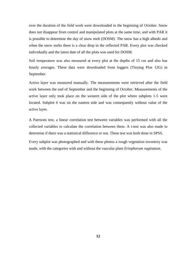
There is a consistent big difference (t-test, p<0,01) between the control and manipulated

plots in emissions, in every round (Figure 8). The manipulated plots have higher

emissions and there is also an increase for every round, and the emissions in the control

plots are decreasing. For control plots the values for round 1, 2 and 3 were

0.16, 0.14 and 0.14 mg CH4 m-2

h-1

and for manipulated the values were

0.51, 0.55 and 0.91 mg CH4 m-2

h-1

. Every dot in the Figure is an average of 36 different

measurements during one round and for the control plots it varied between -0.02

0

0,1

0,2

0,3

0,4

0,5

0,6

0,7

0,8

mg

CH

4 m

-2 h

-1

Total average for CH4 emissions in control and manipulated plots

Control

Manipulated

14

(negative numbers is an uptake) and 0.93 mg CH4 m-2

h-1

and for manipulated plots it was

from -0.03 to 5.51 mg CH4 m-2

h-1

.

Figure 8: The average CH4 flux for every round.

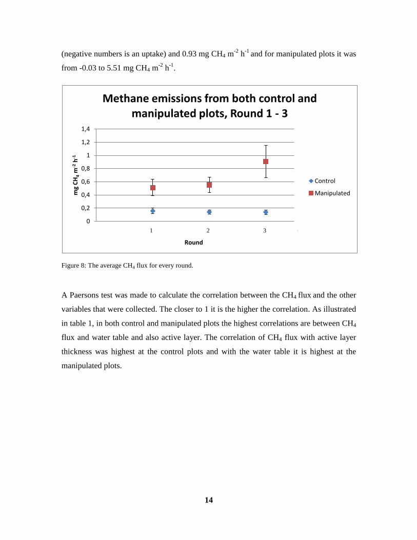
A Paersons test was made to calculate the correlation between the CH4 flux and the other

variables that were collected. The closer to 1 it is the higher the correlation. As illustrated

in table 1, in both control and manipulated plots the highest correlations are between CH4

flux and water table and also active layer. The correlation of CH4 flux with active layer

thickness was highest at the control plots and with the water table it is highest at the

manipulated plots.

0

0,2

0,4

0,6

0,8

1

1,2

1,4

0 0,5 1 1,5 2 2,5 3 3,5

mg

CH

4 m

-2 h

-1

Round

Methane emissions from both control and manipulated plots, Round 1 - 3

Control

Manipulated

1 2 3

15

Table 1: Paersons correlation values between methane flux and different parameters and the number of

corresponding measurements in control and manipulated plots. Also the p-value is presented, and when the

value is below 0.05 it means that it is statistical significant.

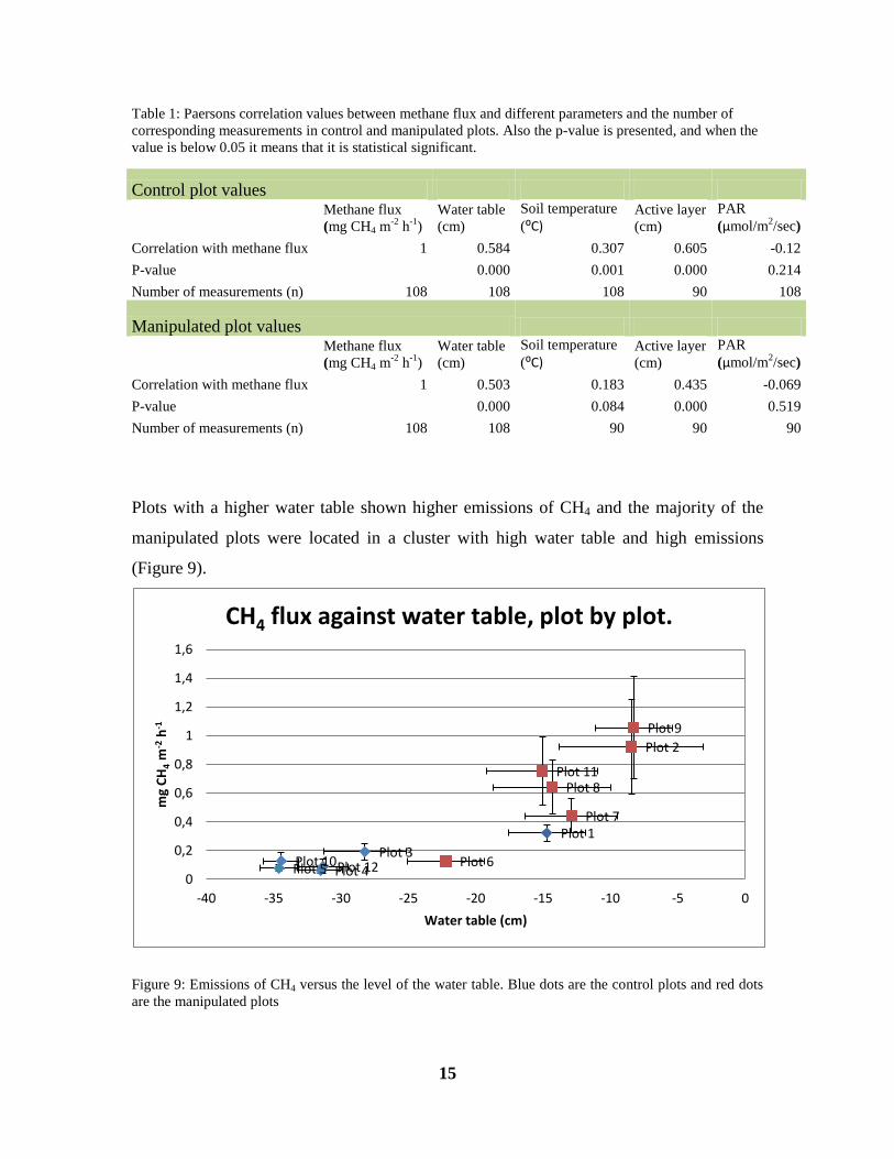
Plots with a higher water table shown higher emissions of CH4 and the majority of the

manipulated plots were located in a cluster with high water table and high emissions

(Figure 9).

Figure 9: Emissions of CH4 versus the level of the water table. Blue dots are the control plots and red dots

are the manipulated plots

Plot 1

Plot 2

Plot 3

Plot 4 Plot 5 Plot 6

Plot 7

Plot 8

Plot 9

Plot 10

Plot 11

Plot 12 0

0,2

0,4

0,6

0,8

1

1,2

1,4

1,6

-40 -35 -30 -25 -20 -15 -10 -5 0

mg

CH

4 m

-2 h

-1

Water table (cm)

CH4 flux against water table, plot by plot.

Control plot values

Methane flux

(mg CH4 m-2

h-1

)

Water table

(cm)

Soil temperature

(⁰C) Active layer

(cm)

PAR

(μmol/m2/sec)

Correlation with methane flux 1 0.584 0.307 0.605 -0.12

P-value

0.000 0.001 0.000 0.214

Number of measurements (n) 108 108 108 90 108

Manipulated plot values

Methane flux

(mg CH4 m-2

h-1

)

Water table

(cm)

Soil temperature

(⁰C) Active layer

(cm)

PAR

(μmol/m2/sec)


P-value

0.000 0.084 0.000 0.519


16

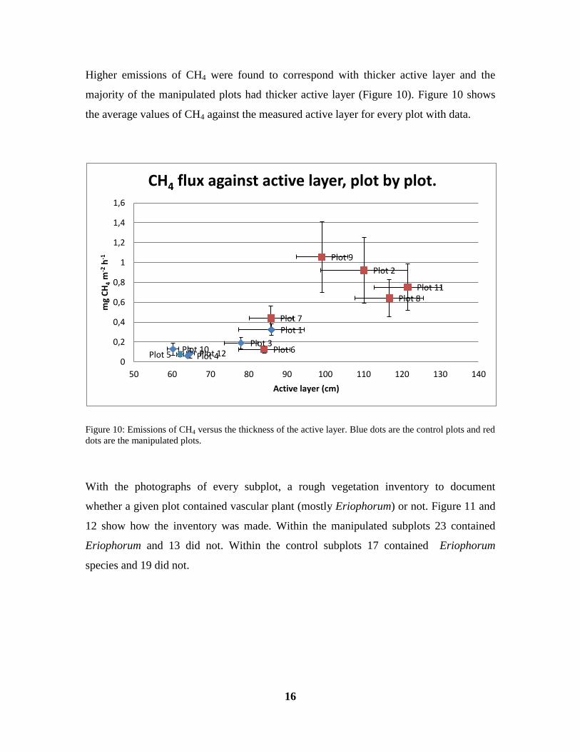
Higher emissions of CH4 were found to correspond with thicker active layer and the

majority of the manipulated plots had thicker active layer (Figure 10). Figure 10 shows

the average values of CH4 against the measured active layer for every plot with data.

Figure 10: Emissions of CH4 versus the thickness of the active layer. Blue dots are the control plots and red

dots are the manipulated plots.

With the photographs of every subplot, a rough vegetation inventory to document

whether a given plot contained vascular plant (mostly Eriophorum) or not. Figure 11 and

12 show how the inventory was made. Within the manipulated subplots 23 contained

Eriophorum and 13 did not. Within the control subplots 17 contained Eriophorum

species and 19 did not.

Plot 1

Plot 2

Plot 3

Plot 4 Plot 5 Plot 6

Plot 7

Plot 8

Plot 9

Plot 10

Plot 11

Plot 12 0

0,2

0,4

0,6

0,8

1

1,2

1,4

1,6

50 60 70 80 90 100 110 120 130 140

mg

CH

4 m

-2 h

-1

Active layer (cm)

CH4 flux against active layer, plot by plot.

17

Figure 11: A few examples of how a subplot could look like when Eriophorum was occurring. From the

left: Subplot 9:2, 11:1 and 2:2.

Figure 12: A few examples of how a subplot could look when Eriophorum was not occurring. From the

left: Subplot 3:2, 2:1 and 5:2.

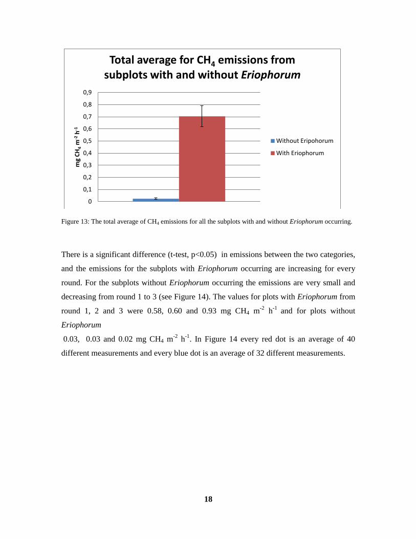
There is a greater difference in CH4 emissions when comparing subplots with and

without Eriophorum, than between manipulated and control plots (Figure 13). Figure 13

shows the total average of CH4 emissions for all the subplots. The subplots where

Eriophorum is occurring had an average flux of 0.70 mg CH4 m-2

h-1

and the subplots

without Eriophorum had an average flux of

0.02 mg CH4 m-2

h-1

.

18

Figure 13: The total average of CH4 emissions for all the subplots with and without Eriophorum occurring.

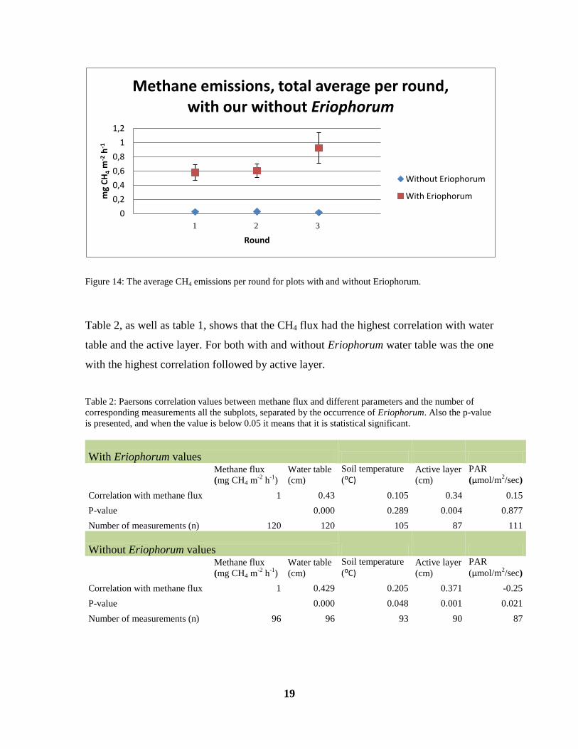
There is a significant difference (t-test, p<0.05) in emissions between the two categories,

and the emissions for the subplots with Eriophorum occurring are increasing for every

round. For the subplots without Eriophorum occurring the emissions are very small and

decreasing from round 1 to 3 (see Figure 14). The values for plots with Eriophorum from

round 1, 2 and 3 were 0.58, 0.60 and 0.93 mg CH4 m-2

h-1

and for plots without

Eriophorum

0.03, 0.03 and 0.02 mg CH4 m-2

h-1

. In Figure 14 every red dot is an average of 40

different measurements and every blue dot is an average of 32 different measurements.

0

0,1

0,2

0,3

0,4

0,5

0,6

0,7

0,8

0,9

mg

CH

4 m

-2 h

-1

Total average for CH4 emissions from subplots with and without Eriophorum

Without Eripohorum

With Eriophorum

19

Figure 14: The average CH4 emissions per round for plots with and without Eriophorum.

Table 2, as well as table 1, shows that the CH4 flux had the highest correlation with water

table and the active layer. For both with and without Eriophorum water table was the one

with the highest correlation followed by active layer.

Table 2: Paersons correlation values between methane flux and different parameters and the number of

corresponding measurements all the subplots, separated by the occurrence of Eriophorum. Also the p-value

is presented, and when the value is below 0.05 it means that it is statistical significant.

With Eriophorum values

Methane flux

(mg CH4 m-2

h-1

)

Water table

(cm)

Soil temperature

(⁰C) Active layer

(cm)

PAR

(μmol/m2/sec)

Correlation with methane flux 1 0.43 0.105 0.34 0.15

P-value

0.000 0.289 0.004 0.877


Without Eriophorum values

Methane flux

(mg CH4 m-2

h-1

)

Water table

(cm)

Soil temperature

(⁰C) Active layer

(cm)

PAR

(μmol/m2/sec)


P-value

0.000 0.048 0.001 0.021


0

0,2

0,4

0,6

0,8

1

1,2

0 1 2 3 4

mg

CH

4 m

-2 h

-1

Round

Methane emissions, total average per round, with our without Eriophorum

Without Eriophorum

With Eriophorum

1 2 3

20

Figure 13 shows very clearly that where Eriophorum species are occurring the CH4

emissions were a lot higher than where they were not, both in control and manipulated

plots. The subplots with Eriophorum also had a higher water table and a thicker active

layer as seen in Figure 15 and 16. Because the categorization with and without

Eriophorum was made on a subplot level the two graphs that follow will not show values

plot by plot, but instead the total average.

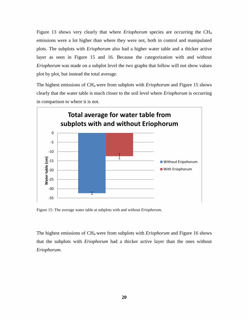
The highest emissions of CH4 were from subplots with Eriophorum and Figure 15 shows

clearly that the water table is much closer to the soil level where Eriophorum is occurring

in comparison to where it is not.

Figure 15: The average water table at subplots with and without Eriophorum.

The highest emissions of CH4 were from subplots with Eriophorum and Figure 16 shows

that the subplots with Eriophorum had a thicker active layer than the ones without

Eriophorum.

-35

-30

-25

-20

-15

-10

-5

0

Wat

er

tab

le (

cm)

Total average for water table from subplots with and without Eriophorum

Without Eripohorum

With Eriophorum

21

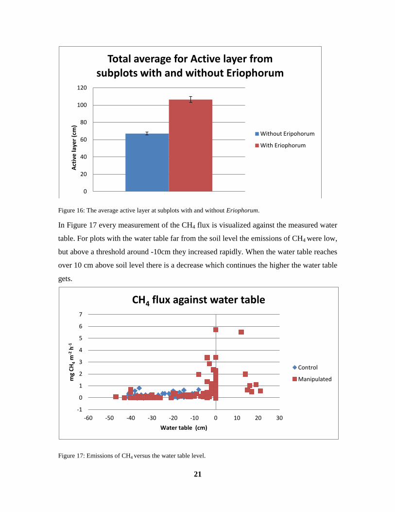
Figure 16: The average active layer at subplots with and without Eriophorum.

In Figure 17 every measurement of the CH4 flux is visualized against the measured water

table. For plots with the water table far from the soil level the emissions of CH4 were low,

but above a threshold around -10cm they increased rapidly. When the water table reaches

over 10 cm above soil level there is a decrease which continues the higher the water table

gets.

Figure 17: Emissions of CH4 versus the water table level.

0

20

40

60

80

100

120

Act

ive

laye

r (c

m)

Total average for Active layer from subplots with and without Eriophorum

Without Eripohorum

With Eriophorum

-1

0

1

2

3

4

5

6

7

-60 -50 -40 -30 -20 -10 0 10 20 30

mg

CH

4 m

-2 h

-1

Water table (cm)

CH4 flux against water table

Control

Manipulated

22

Discussion

Permafrost

The permafrost on this mire is classified as ecosystem protected (Johansson et al. 2011),

and according to Shur and Jorgensson (2007) ecosystem protected permafrost exists

where the mean annual air temperature is approximately 2⁰C to -2⁰C, which matches well

with Storflaket. However, according to Sælthun and Barkved (2003), there will be a 3⁰C

increase of the mean annual air temperature by 2050 and 4.5⁰C by 2080. In Abisko the

mean annual air temperature has been -0.6⁰C (1913-2006), but during the last decade

temperatures have increased. This has put the mean annual air temperature at positive

degrees (Johansson et al. 2011; Callaghan et al. 2010). With these predictions and

considering today’s mean temperature, it is not likely for these permafrost

areas around Abisko to survive.

Equipment

Due to technical issues causing problems with the real-time display of the concentrations,

a duration time of ten minutes was used during the measurements. If the subplot had a

very low flux, a longer measurement time was needed to estimate the flux with a proper

precision. Before the technical malfunction, when visual aid was lost, the longest

duration used was 25 minutes, more than twice as long as the predetermined 10 minutes.

Hence a few measurements may not be totally accurate. This problem, however, was

actual for subplots with very low fluxes, and therefore the absolute error in the

determined flux values was small and could not change the conclusion of the study.

The active layer measurements were conducted by several different people on different

occasions. This may have an impact on the measurement accuracy since different people

may use different ways of measuring. Also some of them were students and may not

23

have experience conducting these kinds of measurements. Still, the overall trend with a

deeper active layer in the manipulated compared with the control plots shown in the data

is considered very solid.

Soil temperature from plot number 9 (Figure 3) and PAR values from plot number 7

(Figure 3) are missing, probably due to faulty equipment.

Methane

To justify the measurements of the field work for this thesis, a comparison was made

between them and the results presented in Lund et al. (2009), who also measured CH4 at

the Storflaket mire. Only mean values of the CH4 fluxes are provided in Lund et al.

(2009), three in total from control plots. Moreover the values are from different seasons.

Two of those were chosen for comparison; summer 0.30 and

autumn 0.45 mg CH4 m-2

h-1

, due to the timing the fieldwork for this thesis. It is also not

known if the control values are from dry or wet areas of the mire. The CH4 fluxes

originating from this thesis are mean values of the data from control plots (0.15 mg CH4

m-2

h-1

) and manipulated plots (0.66 mg CH4 m-2

h-1

). Combining those two gives a mean

value of 0.40 mg CH4 m-2

h-1

. The measurements from this study are therefore within the

span of Lund et al.'s (2009) measurements.

Our study shows that summertime CH4 emissions are higher at locations where snow was

accumulated in winter. In the manipulated plots it was easy to see with the naked eye

how the snow has affected the ground. All of the manipulated plots have a large degraded

part in the middle, an area in which the snow has been deepest. Figure 10 shows clearly

that the active layer is thicker in the manipulated plots. However, in the control plots

there has also been some degradation of permafrost, especially in plot number 1. This can

perhaps be explained by the fact that the annual temperature in the area has been positive

the last decade (seen in Figure 2). The fact that plot 1 is located close to the border of the

mire could also be an aspect of this degradation.

The increased active layer means that the upper part of the permafrost has thawed and the

ice lenses within it have melted, causing a "gap" in the soil, which most of the time is

24

filled with water. This can be seen in Figure 9 where the average height of the water table

is shown plot by plot, and again the manipulated plots have the highest water table.

Johansson et al. (2013) show that the snow between the period of 2005 and 2013 began to

fall around mid October and mid November and the start date is similar in all of the plots.

However, over the years there has been a variation when the snow starts to melt, and the

time difference of snow melt between control and manipulated plots. In 2007, 2008 and

2011 the snow disappeared three weeks later from the manipulated plots than in the

control plots, but in 2012 there was only three days in between. This year the snow

disappeared from the control plots around the 10th of May and from the manipulated

plots around 25th of May, a little more than two weeks difference. Snow depths

measurements from Abisko research station were used as a reference for, when the snow

disappeared from the station. They have ten different plots they measure snow depths in,

and the DOSM is determined when there is no snow left in any of them, which was the

27th of May. But the Swedish Metrological and Hydrological Institute (SMHI) have

determined the DOSM in Abisko to the 18th of May. Using empirical calculations with

the average CH4 fluxes from both control (0.15 mg CH4 m-2

h-1

) and manipulated (0.66

mg CH4 m-2

h-1

) plots during the fieldwork, it will only take around 4 days until the

manipulated plots have emitted the same quantity that the control plots have during 2

weeks. Because of the manipulated plots emits more than four times CH4 than control, it

is easy to assume that the accumulative emissions from the manipulated plots will be

much higher, despite a shorter growing period and different fluxes for spring and autumn.

Two previous studies from a nearby mire(Jackowicz-Korczyński et al. 2010; Johansson

et al. 2006b) have reported that there are higher emissions of CH4 from wetter parts

which is a direct response to permafrost degradation. They both studied a mire named

Stordalen, which is located approximately three kilometres east of the mire Storflaket.

A statistical use of the Pearson test was conducted to quantify the correlation between all

the variables collected at the mire. The largest correlation is between CH4 flux and water

table and active layer as seen in table 1. It is not a surprise that the water table is an

important driver as this has been shown repeatedly in the literature. The water table is a

major regulator of the CH4 production (Bellisario et al. 1999; Christensen et al. 1995;

25

Whalen 2005). However in the same studies soil temperature was shown to be another

factor, which was not seen in this study. This is probably due to the short duration of the

measurement campaign in the current study.

Vascular plants

Due to the predetermined grid of the subplots inside the plots, the subplots did not have

the same conditions as the average of the whole plot. To account for this, the rough

vegetation inventory of every subplot individually was made because the water table and

the thickness of the active layer have a great impact on the vegetation. When the

permafrost thaws it releases nutrients that were frozen in the soil, that is becoming

available for plants. Theoretically the amount of released nutrients is very high because

just below the thaw-front there are nutrients that have been leached from the active layer

into the frozen layer at the end of the summer. When the active layer increases due to

global warming (or snow manipulation), those nutrients are free for the vegetation

(Keuper et al. 2012). This could be an explanation for the quick increase of vascular

plants biomass in areas where the permafrost is disappearing. Also when permafrost

thaws, the area can become wetter or drier depending on how the hydrology is affected

(Christensen 2014). On the Storflaket mire, the majority of the manipulated subplots and

some of the control subplots became wetter.

In the majority of the wet subplots, a vascular plant family named Eriophorum was

identified. Every subplot that had such vascular plants was put in the category with

Eriophorum, although in some of the subplots this was not the dominating species.

Eriophorum species thrive in these wet habitats, especially when the permafrost is

disappearing (Ström et al. 2015), which is seen in Figure 15 and 16. Eriophorum species

show a strong relation to increased CH4 emissions, which can be explained by the fact

that Eriophorum species have a high gross primary production (GPP) (Ström et al. 2015).

Emissions of CH4 are higher in areas with Eriophorum than without (Figure 13) at the

Storflaket mire, but it is not clear if this is because of the higher gross primary production

or the fact that the Eriophorum species thrives in areas where CH4 emissions already are

26

high. Eriophorum may also increase the emissions of CH4 to the atmosphere due to the

fact that they can act as a "chimney" for CH4 and bypass the oxidation horizon, where a

large portion of the CH4 usually is oxidized (Christensen et al. 2000; Macdonald et al.

1998). In wetlands, with, for example, dominating vegetation like Sphagnum, diffusion is

the most common pathway for CH4. During diffusion a large portion of the produced

methane is oxidized (Mastepanov et al. 2012). It is not only the Eriophorum species that

has this "chimney" effect, but in fact most of the vascular plants. Depending on the

species, the level of efficiency can vary (Joabsson et al. 1999).

(Ström et al. 2005) measured the emissions of methane from peatland monoliths with

different dominating vegetation, and one of them was Eriophorum. It was experimental

and the monoliths were kept under constant light and temperature and a high water table

over the duration of the experiment. They measured the average CH4 flux to 2.38 mg CH4

m-2

h-1

. The flux measurements originating from this thesis where Eriophorum was

occurring and the water table was high the average flux was 1.41 mg CH4 m-2

h-1

, which

is not that much lower. The average flux in this study was measured during cold

temperature, cloudy skies and small amounts of rain, not the most favourable conditions

for emissions.

Before the industrial revolution the atmospheric CH4 was around 715ppb, but in 2005 it

was up in 1774ppb which is an increase of 148% and it the greatest increase of all the

greenhouse gases (Forster et al. 2007). For comparison, CO2 only increased 35% over the

same time period (Miao et al. 2012). The majority of the methane emissions is man-

made, but wetlands are the greatest single emission, accounting for around 20% of the

global CH4 budget (Christensen et al. 2003b; Jackowicz-Korczyński et al. 2010; Miao et

al. 2012). As seen in both Figure 9 and 17 there is an exponential increase of CH4

emissions from when the water table is 10 cm below surface and increasing. When the

water table is over 10 cm above ground there is a decrease of the emissions again. This is

shown in Figure 17, and not in Figure 9. That is why Figure 17 is shown, so that will not

be an assumption from Figure 9 that the exponential increase will continue. When the

water table is higher than 10 cm above the soil other processes in the wetlands take over

which favours oxidation (Mastepanov et al. 2012). This is called the water table on/off-

27

switch (Christensen et al. 2003b) and during large scale variations of CH4 emissions this

on/off-switch is very important (Mastepanov et al. 2012).

To be able to make projections of Earth's climate changes we must learn more about the

global budget of CH4 (Miao et al. 2012). For instance, it is not possible today to predict if

an area is becoming wetter or drier when permafrost thaws (Christensen 2014). This is an

important process regarding if the decomposition will produce CH4 or CO2. Also if a wet

area where high emissions of CH4 occurs becomes wetter the emissions can decrease.

This can work the other way around as well; a very wet area that becomes drier

substantially increases the emissions because the water table is now inside the -10 +10

span from the soil surface.

Conclusions

There is a substantial difference between the emissions of CH4 from the control and the

manipulated plots with the latter showing much higher fluxes. Probably one of the main

factors effecting the emissions is the presence of the Eriophorum species in the plots with

artificially increased snow depth.

Accumulative emissions of CH4 are also much higher for manipulated plots than the

control plots over a growing season, despite that the season for the manipulated is shorter.

28

References

Aerts, R., J. H. C. Cornelissen, and E. Dorrepaal. 2006. Plant Performance in a Warmer

World: General Responses of Plants from Cold, Northern Biomes and the

Importance of Winter and Spring Events. 63. DOI: 10.1007/s11258-005-9031-1

AMAP. 2012. Arctic Climate Issues 2011: Changes in Arctic Snow, Water, Ice and

Permafrost. SWIPA 2011 Overview Report. Arctic Monitoring and Assessment

Programme (AMAP). Oslo. xi + 97pp.

Bellisario, L., J. Bubier, T. Moore, and J. Chanton. 1999. Controls on CH4 emissions

from a northern peatland. Global Biogeochem. Cycles, 13: 81-91. DOI:

10.1029/1998GB900021

Bosiö, J., M. Johansson, T. Callaghan, B. Johansen, and T. Christensen. 2012. Future

vegetation changes in thawing subarctic mires and implications for greenhouse

gas exchange-a regional assessment. Climatic Change, 115: 379-398. DOI:

10.1007/s10584-012-0445-1

Bosiö, J., C. Stiegler, M. Johansson, H. Mbufong, and T. Christensen. 2014. Increased

photosynthesis compensates for shorter growing season in subarctic tundra—

8 years of snow accumulation manipulations. Climatic Change, 127: 321-334.

DOI: 10.1007/s10584-014-1247-4

Bosiö, J. A. 2013. A green future with thawing permafrost mires? : a study of climate-

vegetation interactions in European subarctic peatlands. PhD Thesis

Bäckstrand, K., P. M. Crill, M. Jackowicz-Korczyñski, M. Mastepanov, T. R.

Christensen, and D. Bastviken. 2009. Annual carbon gas budget for a subarctic

peatland, northern Sweden. Biogeosciences Discussions, 6: 5705. DOI:

10.5194/bg-7-95-2010

Callaghan, T., M. Johansson, R. Brown, P. Groisman, N. Labba, V. Radionov, R.

Bradley, S. Blangy, et al. 2011. Multiple Effects of Changes in Arctic Snow

Cover. AMBIO - A Journal of the Human Environment, 40: 32-45. DOI:

10.1007/s13280-011-0213-x

Callaghan, T. V., F. Bergholm, T. R. Christensen, C. Jonasson, U. Kokfelt, and M.

Johansson. 2010. A new climate era in the sub-Arctic: Accelerating climate

changes and multiple impacts. Geophysical Research Letters, 37: L14705. DOI:

10.1029/2009gl042064

Christensen, T. A., T. A. Friborg, M. A. Sommerkorn, J. A. Kaplan, L. A. Illeris, H. A.

Sögaard, C. A. Nordström, S. A. Jonasson, et al. 2000. Trace gas exchange in a

high-arctic valley 1. Variations in CO2 and CH4 flux between tundra vegetation

types. Global Biogeochemical Cycles: 701. DOI: 10.1029/1999GB001134

Christensen, T. R. 2014. Climate science: Understand Arctic methane variability. Nature,

509: 279-281.

Christensen, T. R., T. Johansson, H. J. Åkerman, M. Mastepanov, N. Malmer, T. Friborg,

P. Crill, and B. H. Svensson. 2004. Thawing sub-arctic permafrost: Effects on

29

vegetation and methane emissions. Geophysical Research Letters, 31: n/a-n/a.

DOI: 10.1029/2003gl018680

Christensen, T. R., S. Jonasson, T. V. Callaghan, and M. Havström. 1995. Spatial

variation in high-latitude methane flux along a transect across Siberian and

European tundra environments. Journal of Geophysical Research. Atmospheres,

100: 21035. DOI: 10.1029/95JD02145

Christensen, T. R., N. Panikov, M. Mastepanov, A. Joabsson, A. Stewart, M. Öquist, M.

Sommerkorn, S. Reynaud, et al. 2003a. Biotic Controls on CO 2 and CH 4

Exchange in Wetlands: A Closed Environment Study. 337. DOI:

http://dx.doi.org/10.1023/A:1024913730848

Christensen, T. R. A., A. A. Ekberg, L. A. Strom, M. A. Mastepanov, N. A. Panikov, O.

A. Mats, B. A. Svensson, H. A. Nykanen, et al. 2003b. Factors controlling large

scale variations in methane emissions from wetlands. Geophysical Research

Letters. DOI: 10.1029/2002GL016848

Forster, P., V. Ramaswamy, P. Artaxo, T. Berntsen, R. Betts, D. W. Fahey, J. Haywood,

J. Lean, et al. 2007. Changes in atmospheric constituents and in radiative forcing.

Chapter 2. In Climate Change 2007. The Physical Science Basis.

Grogan, P. 2012. Cold Season Respiration Across a Low Arctic Landscape: the Influence

of Vegetation Type, Snow Depth, and Interannual Climatic Variation. Arctic,

Antarctic, and Alpine Research, 44: 446-456. DOI: 10.1657/1938-4246-44.4.446

Hugelius, G. A. 2009. Soil organic carbon in permafrost terrain: Total storage, landscape

distribution and environmental controls. PhD Thesis

Høye, T. T., E. Post, H. Meltofte, N. M. Schmidt, and M. C. Forchhammer. 2007. Rapid

advancement of spring in the High Arctic. Current Biology, 17: R449-R451. DOI:

http://dx.doi.org/10.1016/j.cub.2007.04.047

IPCC. 2014. Summary for Policymakers. In Climate Change 2014: Impacts, Adaptation,

and Vulnerability. Part A: Global and Sectoral Aspects. Contribution of Working

Group II to the Fifth Assessment Report of the Intergovernmental Panel on

Climate Change, eds. C. B. Field, V. R. Barros, D. J. Dokken, K. J. Mach, M. D.

Mastrandrea, T. E. Bilir, M. Chatterjee, K. L. Ebi, Y. O. Estrada, R. C. Genova,

B. Girma, E. S. Kissel, A. N. Levy, S. MacCracken, P. R. Mastrandrea, and L. L.

White, 1-32 pp. Cambridge, United Kingdom, and New York, NY, USA:

Cambridge University Press.

Jackowicz-Korczyński, M., T. R. Christensen, K. Bäckstrand, P. Crill, T. Friborg, M.

Mastepanov, and L. Ström. 2010. Annual cycle of methane emission from a

subarctic peatland. Journal of Geophysical Research: Biogeosciences, 115: n/a-

n/a. DOI: 10.1029/2008jg000913

Joabsson, A., T. R. Christensen, and B. Wallén. 1999. Review: Vascular plant controls on

methane emissions from northern peatforming wetlands. Trends in Ecology &

Evolution, 14: 385-388. DOI: 10.1016/s0169-5347(99)01649-3

Johansson, M., T. V. Callaghan, J. Bosiö, J. Åkerman, M. Jackowicz-Korczynski, and T.

Christensen. 2013. Rapid responses of permafrost and vegetation to

30

experimentally increased snow cover in sub-arctic Sweden. DOI: 10.1088/1748-

9326/8/3/035025

Johansson, M., T. R. Christensen, H. J. Akerman, and T. V. Callaghan. 2006a. What

Determines the Current Presence or Absence of Permafrost in the Torneträsk

Region, a Sub-arctic Landscape in Northern Sweden? AMBIO - A Journal of the

Human Environment, 35: 190-197. DOI: http://dx.doi.org/10.1579/0044-

7447(2006)35[190:WDTCPO]2.0.CO;2

Johansson, M. A., J. A. Åkerman, F. A. Keuper, T. A. Christensen, H. A. Lantuit, T. A.

Callaghan, N. B.-g. v. G. I. I. I. f. n. o. e. P. Lunds universitet, S. S. o. B. Lund

University, et al. 2011. Past and present permafrost temperatures in the Abisko

area: redrilling of boreholes. AMBIO: 558. DOI: 10.1007/s13280-011-0163-3

Johansson, T., N. Malmer, P. M. Crill, T. Friborg, J. H. ÅKerman, M. Mastepanov, and

T. R. Christensen. 2006b. Decadal vegetation changes in a northern peatland,

greenhouse gas fluxes and net radiative forcing. Global Change Biology, 12:

2352-2369. DOI: 10.1111/j.1365-2486.2006.01267.x

Keuper, F., P. M. Bodegom, E. Dorrepaal, J. T. Weedon, J. Hal, R. S. P. Logtestijn, and

R. Aerts. 2012. A frozen feast: thawing permafrost increases plant-available

nitrogen in subarctic peatlands. Global Change Biology, 18: 1998-2007. DOI:

10.1111/j.1365-2486.2012.02663.x

Kip, N., J. F. van Winden, Y. Pan, L. Bodrossy, G.-J. Reichart, A. J. Smolders, M. S.

Jetten, J. S. S. Damsté, et al. 2010. Global prevalence of methane oxidation by

symbiotic bacteria in peat-moss ecosystems. Nature Geoscience, 3: 617-621.

DOI: 10.1038/ngeo939

Liebner, S., J. Zeyer, D. Wagner, C. Schubert, E.-M. Pfeiffer, and C. Knoblauch. 2011.

Methane oxidation associated with submerged brown mosses reduces methane

emissions from Siberian polygonal tundra. Journal of Ecology, 99: 914-922. DOI:

10.1111/j.1365-2745.2011.01823.x

Lund, M., T. R. Christensen, M. Mastepanov, A. Lindroth, and L. Ström. 2009. Effects of

N and P fertilization on the greenhouse gas exchange in two nutrient-poor

peatlands. Biogeosciences Discussions, 6: 4803. DOI: 10.5194/bg-6-2135-2009

Macdonald, J. A., D. Fowler, K. J. Hargreaves, U. Skiba, I. D. Leith, and M. B. Murray.

1998. Methane emission rates from a northern wetland; response to temperature,

water table and transport. Atmospheric Environment, 32: 3219-3227. DOI:

http://dx.doi.org/10.1016/S1352-2310(97)00464-0

Mastepanov, M., C. Sigsgaard, T. Tagesson, L. Ström, M. P. Tamstorf, M. Lund, and T.

R. Christensen. 2012. Revisiting factors controlling methane emissions from high-

arctic tundra. Biogeosciences Discussions: 15853. DOI: 10.5194/bg-10-5139-

2013

McCalley, C. A., B. A. Woodcroft, S. A. Hodgkins, R. A. Wehr, E.-H. A. Kim, R. A.

Mondav, P. A. Crill, J. A. Chanton, et al. 2014. Methane dynamics regulated by

microbial community response to permafrost thaw. Nature: 478. DOI:

10.1038/nature13798

31

Miao, Y., C. Song, L. Sun, X. Wang, H. Meng, and R. Mao. 2012. Growing season

methane emission from a boreal peatland in the continuous permafrost zone of

Northeast China: effects of active layer depth and vegetation. Biogeosciences:

4455. DOI: 10.5194/bg-9-4455-2012

Norina, E. 2007. Methane emissions from northern wetlands. Term paper.

Nykänen, H., J. E. P. Heikkinen, L. Pirinen, K. Tiilikainen, and P. J. Martikainen. 2003.

Annual CO2 exchange and CH4 fluxes on a subarctic palsa mire during

climatically different years. Global Biogeochemical Cycles, 17: n/a. DOI:

10.1029/2002GB001861

Sælthun, N. R., and L. Barkved. 2003. Climate change scenarios for the SCANNET

region.

Schaefer, K., H. Lantuit, V. Romanovsky, and E. Schuur. 2012. Policy implications of

warming permafrost.

Seinfeld, J. H., and S. N. Pandis. 2006. Atmospheric chemistry and physics : from air

pollution to climate change. Hoboken, N.J. : Wiley, cop. 2006

Seppälä, M. 2003. An experimental climate change study of the effect of increasing snow

cover on active layer formation of a palsa, Finnish Lapland. In Proceedings of the

Eighth International Conference on Permafrost, 1013-1016.

Seppälä, M. 2005. The physical geography of Fennoscandia. Oxford : Oxford University

Press, 2005.

Shur, Y. L., and M. T. Jorgenson. 2007. Patterns of permafrost formation and degradation

in relation to climate and ecosystems. Permafrost & Periglacial Processes, 18: 7.

DOI: 10.1002/ppp.582

Ström, L., and T. R. Christensen. 2007. Below ground carbon turnover and greenhouse

gas exchanges in a sub-arctic wetland. Soil Biology and Biochemistry, 39: 1689-

1698. DOI: http://dx.doi.org/10.1016/j.soilbio.2007.01.019

Ström, L., J. Falk, K. Skov, M. Jackowicz-Korczynski, M. Mastepanov, T. Christensen,

M. Lund, and N. Schmidt. 2015. Controls of spatial and temporal variability in

CH flux in a high arctic fen over three years. Biogeochemistry, 125: 21-35. DOI:

10.1007/s10533-015-0109-0

Ström, L., M. Mastepanov, and T. R. Christensen. 2005. Species-Specific Effects of

Vascular Plants on Carbon Turnover and Methane Emissions from Wetlands. 65.

DOI: 10.1007/s10533-004-6124-1

Svensson, B. H., T. R. Christensen, E. Johansson, and M. Öquist. 1999. Interdecadal

Changes in CO2 and CH4 Fluxes of a Subarctic Mire: Stordalen Revisited after

20 Years. Oikos, 85: 22-30. DOI: 10.2307/3546788

Whalen, S. C. 2005. Biogeochemistry of Methane Exchange between Natural Wetlands

and the Atmosphere. Environmental Engineering Science, 22: 73-94. DOI:

10.1089/ees.2005.22.73

32

WMO. 2015. The State of Greenhouse Gases in the Atmosphere Based on Global

Observations through 2014. WMO GREENHOUSE GAS BULLETIN.

Åkerman, H. J., and M. Johansson. 2008. Thawing permafrost and thicker active layers in

sub-arctic Sweden. Permafrost and Periglacial Processes, 19: 279-292. DOI:

10.1002/ppp.626

33

Institutionen för naturgeografi och ekosystemvetenskap, Lunds Universitet.

Student examensarbete (Seminarieuppsatser). Uppsatserna finns tillgängliga på

institutionens geobibliotek, Sölvegatan 12, 223 62 LUND. Serien startade 1985. Hela

listan och själva uppsatserna är även tillgängliga på LUP student papers

(https://lup.lub.lu.se/student-papers/search/) och via Geobiblioteket (www.geobib.lu.se)

The student thesis reports are available at the Geo-Library, Department of Physical

Geography and Ecosystem Science, University of Lund, Sölvegatan 12, S-223 62 Lund,

Sweden. Report series started 1985. The complete list and electronic versions are also

electronic available at the LUP student papers (https://lup.lub.lu.se/student-

papers/search/) and through the Geo-library (www.geobib.lu.se)

335 Fei Lu (2015) Compute a Crowdedness Index on Historical GIS Data- A Case

Study of Hög Parish, Sweden, 1812-1920

336 Lina Allesson (2015) Impact of photo-chemical processing of dissolved

organic carbon on the bacterial respiratory quotient in aquatic ecosystems

337 Andreas Kiik (2015) Cartographic design of thematic polygons: a comparison

using eye-movement metrics analysis

338 Iain Lednor (2015) Testing the robustness of the Plant Phenology Index to

changes in temperature

339 Louise Bradshaw (2015) Submerged Landscapes - Locating Mesolithic

settlements in Blekinge, Sweden

340 Elisabeth Maria Farrington (2015) The water crisis in Gaborone: Investigating

the underlying factors resulting in the 'failure' of the Gaborone Dam, Botswana

341 Annie Forssblad (2015) Utvärdering av miljöersättning för odlingslandskapets

värdefulla träd

342 Iris Behrens, Linn Gardell (2015) Water quality in Apac-, Mbale- & Lira

district, Uganda - A field study evaluating problems and suitable solutions

343 Linnéa Larsson (2015) Analys av framtida översvämningsrisker i Malmö - En

fallstudie av Castellums fastigheter

34

344 Ida Pettersson (2015) Comparing Ips Typographus and Dendroctonus

ponderosas response to climate change with the use of phenology models

345 Frida Ulfves (2015) Classifying and Localizing Areas of Forest at Risk of

Storm Damage in Kronoberg County

346 Alexander Nordström (2015) Förslag på dammar och skyddsområde med hjälp

av GIS: En studie om löv- och klockgroda i Ystad kommun, Skåne

347 Samanah Seyedi-Shandiz (2015) Automatic Creation of Schematic Maps - A

Case Study of the Railway Network at the Swedish Transport Administration

348 Johanna Andersson (2015) Heat Waves and their Impacts on Outdoor Workers

– A Case Study in Northern and Eastern Uganda

349 Jimmie Carpman (2015) Spatially varying parameters in observed new particle

formation events

350 Mihaela – Mariana Tudoran (2015) Occurrences of insect outbreaks in Sweden

in relation to climatic parameters since 1850

351 Maria Gatzouras (2015) Assessment of trampling impact in Icelandic natural

areas in experimental plots with focus on image analysis of digital photographs

352 Gustav Wallner (2015) Estimating and evaluating GPP in the Sahel using

MSG/SEVIRI and MODIS satellite data

353 Luisa Teixeira (2015) Exploring the relationships between biodiversity and

benthic habitat in the Primeiras and Segundas Protected Area, Mozambique

354 Iris Behrens & Linn Gardell (2015) Water quality in Apac-, Mbale- & Lira

district, Uganda - A field study evaluating problems and suitable solutions

355 Viktoria Björklund (2015) Water quality in rivers affected by urbanization: A

Case Study in Minas Gerais, Brazil

356 Tara Mellquist (2015) Hållbar dagvattenhantering i Stockholms stad - En

riskhanteringsanalys med avseende på långsiktig hållbarhet av Stockholms

stads dagvattenhantering i urban miljö

357 Jenny Hansson (2015) Trafikrelaterade luftföroreningar vid förskolor – En

studie om kvävedioxidhalter vid förskolor i Malmö

358 Laura Reinelt (2015) Modelling vegetation dynamics and carbon fluxes in a

high Arctic mire

35

359 Emelie Linnéa Graham (2015) Atmospheric reactivity of cyclic ethers of

relevance to biofuel combustion

360 Filippo Gualla (2015) Sun position and PV panels: a model to determine the

best orientation

361 Joakim Lindberg (2015) Locating potential flood areas in an urban

environment using remote sensing and GIS, case study Lund, Sweden

362 Georgios-Konstantinos Lagkas (2015) Analysis of NDVI variation and

snowmelt around Zackenberg station, Greenland with comparison of ground

data and remote sensing.

363 Carlos Arellano (2015) Production and Biodegradability of Dissolved Organic

Carbon from Different Litter Sources

364 Sofia Valentin (2015) Do-It-Yourself Helium Balloon Aerial Photography -

Developing a method in an agroforestry plantation, Lao PDR

365 Shirin Danehpash (2015) Evaluation of Standards and Techniques for

Retrieval of Geospatial Raster Data - A study for the ICOS Carbon Portal

366 Linnea Jonsson (2015) Evaluation of pixel based and object based

classification methods for land cover mapping with high spatial resolution

satellite imagery, in the Amazonas, Brazil.

367 Johan Westin (2015) Quantification of a continuous-cover forest in Sweden

using remote sensing techniques

368 Dahlia Mudzaffar Ali (2015) Quantifying Terrain Factor Using GIS

Applications for Real Estate Property Valuation

369 Ulrika Belsing (2015)The survival of moth larvae feeding on different plant

species in northern Fennoscandia

370 Isabella Grönfeldt (2015) Snow and sea ice temperature profiles from satellite

data and ice mass balance buoys

371 Karolina D. Pantazatou (2015) Issues of Geographic Context Variable

Calculation Methods applied at different Geographic Levels in Spatial

Historical Demographic Research -A case study over four parishes in Southern

Sweden

372 Andreas Dahlbom (2016) The impact of permafrost degradation on methane

36

fluxes - a field study in Abisko

The impact of permafrost degradation on methane...

Documents

Transcript of The impact of permafrost degradation on methane...