1

Published in The Monthly Notices of the Royal Astronomical Society vol. 477, 4,

4627-4640

The Ice Cap Zone: A Unique Habitable Zone for Ocean

Worlds

Ramses M. Ramirez1 and Amit Levi2

1Earth-Life Science Institute, Tokyo Institute of Technology, 2-12-1, Tokyo, Japan

152-8550 2 Harvard-Smithsonian Center for Astrophysics, 60 Garden Street, Cambridge, MA

02138, USA

email: rramirez@elsi.jp

ABSTRACT

Traditional definitions of the habitable zone assume that habitable planets contain a carbonate-

silicate cycle that regulates CO2 between the atmosphere, surface, and the interior. Such theories

have been used to cast doubt on the habitability of ocean worlds. However, Levi et al (2017)

have recently proposed a mechanism by which CO2 is mobilized between the atmosphere and the

interior of an ocean world. At high enough CO2 pressures, sea ice can become enriched in CO2

clathrates and sink after a threshold density is achieved. The presence of subpolar sea ice is of

great importance for habitability in ocean worlds. It may moderate the climate and is

fundamental in current theories of life formation in diluted environments. Here, we model the

Levi et al. mechanism and use latitudinally-dependent non-grey energy balance and single-

column radiative-convective climate models and find that this mechanism may be sustained on

ocean worlds that rotate at least 3 times faster than the Earth. We calculate the circumstellar

region in which this cycle may operate for G-M-stars (Teff = 2,600 – 5,800 K), extending from

~1.23 - 1.65, 0.69 - 0.954, 0.38 – 0.528 AU, 0.219 – 0.308 AU, 0.146 – 0.206 AU, and 0.0428 –

0.0617 AU for G2, K2, M0, M3, M5, and M8 stars, respectively. However, unless planets are

very young and not tidally-locked, our mechanism would be unlikely to apply to stars cooler than

a ~M3. We predict C/O ratios for our atmospheres (~0.5) that can be verified by the JWST

mission.

Key words: astrobiology – planets and satellites: atmospheres – planets and satellites: oceans -

stars: low-mass

2

1. INTRODUCTION

In this work, we focus on ocean worlds.

These are defined here as: (1) exoplanets with

tens of percent of their total mass composed

of water that (2) lack a substantial H/He

envelope and (3) have migrated close enough

to their host star so that their outermost

condensed mantle is a global ocean.

Accretion of a few percent by mass of

water is sufficient to form a barrier,

composed of high-pressure water ice

polymorphs, between the rocky inner mantle

and the ocean (Levi, Sasselov & Podolak,

2014). A high mass fraction of water may be

explained by forming the planet beyond the

snowline (Kuchner 2003) (L ́eger, et al.

2004). Photo-evaporation of the H/He

atmosphere places an upper bound on the

planetary core mass of about 2M⨁ (Luger, et

al. 2015). However, a low mass planet

forming beyond the snowline implies a low

mass disk, which is associated with low mass

stars. Using population synthesis models,

Alibert & Benz (2017) have shown that

water-rich planets as defined here are a

natural outcome around very low mass (~ M

spectral class) stars. The abundance of low

mass stars and the ubiquity of water in solar

systems suggest our studied planets should be

very common, with implications for near

future observations. We note that M-class

stars experience a particularly large

migration in their snow line, likely affecting

the formation of water rich planets. This issue

continues to be studied, however. Another

substantial unknown is the retention of water

during high-impact collisions. Plus, recent

planet formation models have largely been

driven by limited observations. Nevertheless,

statistics suggests that ocean worlds may be

common throughout the cosmos (Simpson,

2017). Given such uncertainties, our search

for the ice cap zone will extend beyond M-

class stars (G-class).

A better understanding of the habitable

zone (HZ) (which is the circular region

around a star where standing bodies of liquid

water could be stable on the surface of a

rocky planet) is required in order to better

guide observations toward planets of

hypothesized biological interest. Even

though not all HZ planets are habitable, the

HZ remains a useful tool for prioritizing

promising targets in the search for

extraterrestrial life. The most popular

incarnation of this concept remains that

devised by Kasting et al. (1993) (and updated

by us in Kopparapu et al. 2013) which posits

that habitable planets have roughly Earth-like

masses, Earth-like surface water inventories,

a carbonate-silicate cycle, and orbit stars in

their main-sequence of stellar evolution.

Another key assumption is that CO2 and H2O

are the main greenhouse gases as they are on

the Earth, leading to H2O-dominated

atmospheres near the inner edge and CO2-

dominated atmospheres near the outer edge.

In what we dub here as the “classical HZ”,

the entire surface water inventory evaporates

and a runaway greenhouse edge ensues at the

inner edge boundary, leading to rapid

desiccation and Venus-like planetary

conditions. In our solar system, this

“runaway greenhouse” limit occurs at ~0.95

AU (Leconte et al., 2013; Kopparapu et al.,

2014; Ramirez & Kaltenegger, 2014;2016).

A more pessimistic inner edge, the moist

greenhouse, occurs when mean surface

temperatures exceed ~340 K, beyond which

a water inventory equal to the amount in

Earth’s oceans is lost to space on a timescale

of ~4.5 Gyr (i.e. the age of the solar

system)(e.g. Kasting et al. 1993). On the

3

other hand, the outer edge of this classical HZ

is the distance beyond which the combined

effects of CO2 condensation and Rayleigh

scattering outweigh its greenhouse effect.

The higher CO2 pressures needed to sustain

warm surface conditions at distances

approaching this outer edge are assumed to

be provided by the carbonate-silicate cycle,

which helps ensure a relatively wide

habitable zone (e.g. Kasting et al. 1993).

Although the classical HZ is a great way

to frame planetary habitability, how well this

particular formulation represents reality is, at

present, unknown and requires continued

study. An ongoing discussion regarding how

representative the underlying assumptions

may be for the habitability of extraterrestrial

planets continues (e.g. Abe et al., 2011; Agol,

2011; Pierrehumbert & Gaidos, 2011;

Seager, 2013; Zsom et al. 2013; Kasting et al.

2014; Ramirez & Kaltenegger, 2014;

2016;2017).

In here, we revisit the notion of the

carbonate-silicate cycle, which regulates the

exchange of CO2 between the interior and the

atmosphere and is thought to be vital in

maintaining clement surface temperatures

over Earth’s geologic history (e.g. Kasting et

al. 1993). Abbot et al. (2012) have argued

that such a cycle can be sustained on worlds

with land fractions as low as 5%. Although

this suggests that the cycle would operate on

planets that have at least some land, it also

indicates that true ocean worlds may be

uninhabitable.

However, studies suggest this may not be the

case. In the absence of a silicate weathering

feedback, atmospheric CO2 concentrations

are expected to build up in ocean worlds (e.g.

Wordsworth and Pierrehumbert, 2013).

Moreover, the resultant CO2 cycle would

exhibit a stabilizing negative feedback with

high CO2 cooling rates favoring lower

atmospheric escape rates (e.g. Wordsworth

and Pierrehumbert, 2013; Kitzmann et al.,

2015).

Clearly then, the classical HZ is

inadequate for describing our studied ocean

worlds. A planet much richer in water than

the Earth (tens of percent of the total

planetary mass) will not likely lose its surface

water inventory in a runaway greenhouse. In

addition, though the carbonate-silicate cycle

is inactive due to the high-pressure ice

barrier, other mechanisms, based on water ice

phase transitions in sea ice, may moderate the

climate (Levi et al. 2017). Thus, the

difference in the geophysical cycles between

rocky planets and ocean worlds merit an

independent definition for the inner and outer

edges of the HZ for the case of ocean worlds.

As explained above, the classical HZ

does not explicitly consider needed

conditions for the evolution of life, besides

the stable existence of liquid water. In this

work, we attempt to incorporate within our

definition of the HZ for ocean worlds

restrictions imposed by prebiotic chemistry

and the initiation of an RNA-world. This, we

expect, should yield a more restrictive, yet

stronger, filter for targeting planets for

observation.

A major concern when considering the

evolution of life on ocean worlds is that the

absence of continents and the deep ocean

yield a globally diluted environment. For

example, formaldehyde and HCN are

important precursors in several synthetic

pathways, known to produce amino acids and

nucleobases, see discussion in Schwartz and

Goverde (1982). Reactions forming amino

acids and nucleobases require a high

concentration of HCN, otherwise hydrolysis

of HCN dominates, resulting in the

production of formate and ammonia.

4

Levy et al. (2000) suggested that when a

diluted aqueous solution freezes, the ice Ih

grains exsolve impurities that become

concentrated within the remaining liquid

pores. The high concentrations obtained

more than offset the lower kinetics at

subfreezing temperatures. The high

concentrations thus achieved can drive

production at high yields. Freezing a 0.1M

solution of NH4CN produces: glycine,

racemic alanine and aspartic acid (Levy, et al.

2000). Sparking an aqueous solution of CH4,

N2 and NH3formed adenine, only upon

freezing to −20oC (Levy, et al. 2000).

Kanavarioti et al. (2001) investigated ice as a

reaction medium using uridine nucleotides.

They found that freezing to −18oC was a

necessary condition for enhanced

oligomerization, with yields decreasing for

higher temperatures. Therefore, frozen

conditions are superior to free liquid

solutions in synthesizing RNA oligomers.

Furthermore, freezing was found to support

and enhance RNA replication without

comprising fidelity, and provide a form of

compartmentalization required by Darwinian

evolution (Attwater, et al. 2010).

However, others suggest that mere

freezing is not sufficient. Menor-Salvan et al.

(2009) found that spark discharges in a

reduced atmosphere highly favored the

production of cytosine and triazine, only

when the system was exposed to a freeze-

thaw cycle (between −5oC and 5oC). In the

absence of a freeze-thaw cycle the production

of tholins was favored. Freeze-thaw cycles

are also needed to help bridge the gap from

the prebiotic chemistry of short RNA

oligomers to complex replicating ribozymes

(Mustschler, Wochner & Holliger, 2015).

In ocean worlds freeze-thaw cycles are

possible where there is a polar ice cap.

Forming sea ice ought to gradually exsolve

impurities into its pores, approaching eutectic

compositions. Thus, providing the necessary

increase in concentrations discussed above.

Further transition of the ice Ih grains into CO2

clathrate hydrate comes at the expense of

pore space, hence increasing the chances of

molecular collisions and reactions. Some sea

ice floes on the periphery of the subpolar

region may dissociate, due to migration to

latitudes with higher surface temperatures,

rather than sink (see discussion in Levi et al.,

2017). It is possible that processed material

released from the pores, following this

dissociation, will refreeze, if returned by

surface currents to higher latitudes.

Hence, pinpointing the heliocentric

region around different types of stars, which

is coincident with the condition of having a

subpolar ice cap, is important. We refer to

this region as the ice cap zone. Planets closer

in are free of sea ice and planets farther out

are snowballs.

Although the work in Levi et al.

(2017) suggests that ocean worlds may be

habitable without the carbonate-silicate

cycle, the ocean model was not coupled to an

atmospheric model to assess the plausibility

of such solutions. Here, we couple the model

in Levi et al. (2017) with a single-column

radiative-convective climate model and an

energy balance climate model developed by

one of us (Ramirez) to determine the location

of the ice cap zone for G- M-stars. In Section

2 we give a brief description of the CO2

ocean-atmospheric exchange modelled in

Levi et al. (2017) and describe the inner and

outer boundaries of the ice cap zone from a

geophysical perspective. The climatological

perspective is given in Section 3.1. In

Sections 3.2 and 3.3 we describe the

radiative-convective and energy balance

climate models used to perform our analyses.

Climate modeling procedures are discussed

in section 3.4. Our Results and Discussion are

5

found in Sections 4 and 5, respectively,

leading to the Conclusion.

2. THE ICE CAP ZONE

For the benefit of the reader the following

is a brief review of the mechanism developed

in Levi et al. (2017), and a recap of a few of

its fundamental governing equations. In Levi

et al. (2017) we have studied different

mechanisms governing the exchange of CO2 between the deep water-rich ice mantle, the

ocean, and the atmosphere (see Fig.1 for an

illustration of our system). We have

suggested that CO2 in the water-rich ice

mantle promotes an ocean floor enriched in

CO2 clathrate hydrates. An ocean under-

saturated in CO2 would cause the dissociation

of these clathrates, and the subsequent release

of CO2 into the ocean, thus reaching

saturation. Therefore, the clathrate phase

controls the CO2 saturation level in the deep

(~100km) global ocean.

Vertical mixing and homogenization of the

oceans here on Earth are powered by tides

and winds. These supply about 1TW, which

is sufficient to support the circulation in

Earth’s oceans (Wunsch, C. & Ferrari, R.

2004; Kuhlbrodt et al. 2007). However, this

power is insufficient for homogenizing the

deep oceans that are the focus of this study,

requiring at least tens of TW (Levi et al.

2017). Winds, however, can support the

circulation of the upper ocean (upper few

kilometers), with implications for CO2

outgassing rates.

A meridional temperature gradient, on a

rotating planet, should give rise to surface

wind patterns that cause the ocean surface

water to diverge and converge. This promotes

circulation in the upper ocean via Ekman

pump and suction (see illustration in Fig.1).

The net outgassing of dissolved CO2into the

atmosphere, due to this circulation, is the

difference between the influx and outflux of

CO2between ocean and atmosphere.

In regions where oceanic surface water

converge, Ekman pumping results in an

influx of atmospheric CO2 of (see eq.53 in

Levi et al. 2017):

𝑗𝐶𝑂2

𝑖𝑛 = [𝛽(𝑇𝑠𝑏𝑡) − 𝛽(𝑇𝑡𝑟𝑜𝑝)]𝑃𝑎𝑡𝑚𝐶𝑂2𝑤𝑒 (1)

Here 𝛽 is a Henry-like constant relating

solubility (dissolved number density of CO2)

to the partial atmospheric pressure of carbon-

dioxide, 𝑃𝑎𝑡𝑚𝐶𝑂2. The vertical velocity in the

circulation is 𝑤𝑒. The subtropical and tropical

oceanic surface temperatures are: 𝑇𝑠𝑏𝑡, and

𝑇𝑡𝑟𝑜𝑝, respectively.

At the bottom of the wind-driven circulation,

the geostrophic flow is in contact with the

deep ocean, which is saturated in CO2.

Therefore, enriching this water with CO2, if it

is under-saturated. The liquid parcels that are

reemerging at the ocean surface, in regions of

surface water divergence, experience

degassing, thus establishing a CO2 outflux of

(see eq.76 in Levi et al. 2017):

𝑗𝐶𝑂2

𝑜𝑢𝑡 = 𝑤𝑒[𝑛𝐶𝑂2

𝑜𝑢𝑡 − 𝛽(𝑇𝑡𝑟𝑜𝑝)𝑃𝑎𝑡𝑚𝐶𝑂2] (2)

where, 𝑛𝐶𝑂2

𝑜𝑢𝑡 is the number density of

CO2dissolved in the enriched water pumped

to the surface via Ekman suction. The latter

is a complex function of time, the vertical

eddy diffusion coefficient for the deep ocean,

the number density of CO2 dissolved in the

deep ocean, the ocean depth, the flux of

circulated water that comes in contact with

the deep unmixed ocean, and the length scale

between regions of surface water

convergence and divergence. These relations

are given in Eqs.71-75 in Levi et al. (2017)

The fluxes due to the wind-driven circulation

6

equilibrate when the number density of CO2

dissolved in surface regions where the ocean

water converges, equals the number density

of dissolved CO2in the saturated deep ocean.

This results in an atmosphere of tens of bars

of CO2 (see Fig.20 in Levi et al. 2017).

However, such an atmosphere is unstable if

anywhere on the surface of the planet

temperatures are lower than about 280K. In

these colder regions, atmospheric CO2, at the

level of a few tens of bars, will convert the

liquid surface water into CO2 clathrate

hydrate, on the expense of the atmospheric

CO2. The clathrate hydrate of CO2 is denser

than the ocean (see Fig.23 in Levi et al.2017),

and is thermodynamically stable in the deep

saturated ocean. Therefore, atmospheric CO2

deposited in these clathrates will sediment to

the bottom of the ocean, thus, lowering the

atmospheric pressure of CO2 toward its

clathrate dissociation pressure (a few bars).

Therefore, a constant tension exists between

two tendencies: on the one hand trying to

equilibrate the atmospheric abundance of

CO2with that which is dissolved in the deep

ocean, while on the other hand sinking any

excess in the atmospheric CO2 above the

clathrate dissociation pressure.

For subpolar temperatures below 250K water

first freezes as ice Ih, which is then converted

over time into a CO2 clathrate hydrate, as

explained above. When a mole fraction,

𝛼𝑚𝑖𝑛, of the original ice ih is transformed into

CO2 clathrate hydrate, the sea-ice composite

becomes denser than the ocean and sinks (see

eq. 89 in Levi et al. 2017). The time elapsed

before a clathrate enrichment of 𝛼𝑚𝑖𝑛 is

reached is a function of the temperature,

pressure and ice grain morphology. The

resulting number of CO2 molecules removed

from the atmosphere, and deposited on the

bottom of the ocean, per unit time is (see eq.

94 in Levi et al. 2017):

𝑑𝑁𝑖𝑐𝑒−𝑠𝑖𝑛𝑘

𝑑𝑡=

2𝜋𝑅𝑝2(1−𝑠𝑖𝑛𝜆𝑠𝑝)ℎ𝑖𝑐𝑒𝜍𝛼𝑚𝑖𝑛(1−𝜙𝑝𝑜𝑟𝑒

0 )

∆𝜏

46

𝑉𝑐𝑒𝑙𝑙

1

5.75

(3)

Here 𝜆𝑠𝑝is the latitudinal extent of the ice

cap, 𝑅𝑝is the planetary radius, ℎ𝑖𝑐𝑒is the

thickness of the sea-ice slab prior to sinking,

𝜙𝑝𝑜𝑟𝑒0 is the initial porosity of the forming

sea-ice, 𝑉𝑐𝑒𝑙𝑙is the unit cell volume of the

clathrate, and 𝜍 is an expansion coefficient

equal to 1.133. ∆𝜏 is the time duration a sea-

ice slab remains afloat, i.e. the time needed to

reach a clathrate enrichment of 𝛼𝑚𝑖𝑛. ∆𝜏 is

restricted by the divergent flow of sea-ice

away from the cold subpolar region (see

eq.103 in Levi et al. 2017). In other words,

sea-ice remaining positively buoyant beyond

this time criterion, may be carried away to

warmer regions, where its clathrate

component may dissociate, consequently

releasing its CO2 content back into the

atmosphere. This restriction on ∆𝜏leads to a

restriction on the ice grain size (We refer the

interested reader to subsection 6.2 in Levi et

al. 2017, for more details and an in-depth

discussion of this issue).

Considering the fluxes above, a steady state

for the partial atmospheric pressure of CO2is

reached over time, which obeys the following

relation (see eq. 102 in Levi et al. 2017):

0 = 𝜋𝑅𝑝𝑁𝑤𝑑𝑐𝛽(𝑇𝑠𝑏𝑡)𝐷𝑒𝑑𝑑𝑦𝐿𝑔

𝐿𝑜𝑐𝑒𝑎𝑛[

𝑛𝐶𝑂2

𝑑𝑒𝑒𝑝

�̃�(𝑇𝑠𝑏𝑡)−

𝑃𝑎𝑡𝑚𝐶𝑂2] − 𝑆𝑤

𝑑𝑁𝑖𝑐𝑒−𝑠𝑖𝑛𝑘

𝑑𝑡− 𝑄𝑐

4𝜋𝑅𝑝2

𝑚𝐶𝑂2𝑔

(4)

The three terms on the right-hand side of the

last equation represent the contributions of:

the wind-driven circulation (i.e. equilibration

with the deep ocean), the sea-ice sink

mechanism, and an external atmospheric

erosion term, respectively. 𝑁𝑤𝑑𝑐 is the

7

number of wind driven circulations, 𝐷𝑒𝑑𝑑𝑦is

the vertical eddy diffusion coefficient for the

deep ocean, 𝐿𝑔is the horizontal length scale

of the circulation, 𝐿𝑜𝑐𝑒𝑎𝑛is the depth of the

ocean, 𝑛𝐶𝑂2

𝑑𝑒𝑒𝑝is the number density of

dissolved CO2in the deep ocean, 𝑚𝐶𝑂2is the

mass of a CO2molecule, 𝑔 is the acceleration

of gravity, and 𝑄𝑐is an external atmospheric

erosion factor having units of pressure over

time.

Figure 1: An illustration of the transport of 𝐶𝑂2between ocean and atmosphere in water-rich

planets. The ocean floor is rich in 𝐶𝑂2clathrate hydrate, which keeps the ocean saturated in 𝐶𝑂2.

Winds drive a circulation of the upper ocean. The circulated water is enriched in 𝐶𝑂2due to the

contact with the deep saturated ocean. This added 𝐶𝑂2is later degassed into the atmosphere

during the suction of deep water. This process strives to outgas tens of bars of 𝐶𝑂2into the

atmosphere. However, this high atmospheric pressure may be unstable. If subpolar temperatures

are subfreezing, then sea-ice is transformed over time from mainly being composed of ice Ih into

a composition rich in the clathrate hydrate of 𝐶𝑂2. A sufficient enrichment in the latter phase

turns the sea-ice floe negatively buoyant. This process tends to clear the atmosphere of any

excess 𝐶𝑂2, thus reducing the global atmospheric pressure of 𝐶𝑂2to the dissociation pressure of

the clathrate phase.

8

Figure 2: The steady-state partial atmospheric pressure of CO2 as a function of the average polar

surface temperature. The vertical axis is the steady-state atmospheric CO2 pressure. The

horizontal axis is the subpolar temperature averaged over the planetary orbit. The following

initial ice Ih grain radii are assumed for the sea ice: 100μm (solid red curve), 200μm (solid cyan

curve) and 300μm (solid magenta curve). The dashed green curve represents the dissociation

pressure of the CO2 clathrate hydrate. The latter phase is stable only above its dissociation curve.

In Fig. 2 (see also Fig.29 in Levi et al. 2017)

we plot solutions for the steady-state partial

atmospheric pressure of CO2 versus the

subpolar temperature. The rate of

transformation from ice Ih into clathrate is

temperature- and pressure-dependent. This

transformation is kinetically fast for the

highest temperatures plotted in Fig. 2.

Therefore, the resulting steady-state

atmospheric pressure is close to the

dissociation curve of the clathrate (green

dashed curve). This is because the sea-ice

sink mechanism is effective. When

considering lower temperatures, for the

subpolar region, the transition between the

ice phases slows down. As a result, sea-ice

can migrate away from the ice cap region to

a warmer climate, and release its CO2content

back into the atmosphere. The increase in

CO2 pressure acts to accelerate the transition

between the phases, counteracting the effect

of the lower temperature. Clearly, the lower

the temperature is, the higher is the

CO2pressure needed to counterbalance the

effect of the former. Thus, a minimum in the

pressure is evident for some subpolar

temperature, depending on the morphology

of the ice grains forming the sea-ice (see Levi

9

et al. 2017 for a discussion on the ice grain

morphology).

In Levi et al. (2017) we have estimated that it

takes thousands of years for the wind-driven

circulation to smooth out disturbances in the

atmospheric pressure from its steady state

value. Near steady state the sea ice sink for

atmospheric CO2 can change the atmospheric

abundance of this chemical species at a rate

of about 2 mbar yr−1. This is assuming the

polar ice cap extends to the 60th parallel and

an initial sea ice porosity of 0.1. The possible

change in atmospheric pressure per year is

much less than the atmospheric pressure

predicted at steady state. Therefore, the

influxes and outfluxes of CO2 are far too low

for the atmosphere to adjust to seasonal

variations in the subpolar temperature.

Hence, in this work, the geophysical model is

coupled with the climate model using a

subpolar temperature which is averaged over

the planetary orbit.

The ice cap zone has an inner and outer edge.

In this section, we wish to address these

edges within a geophysical context. We

discuss this issue further within a

climatological context below (See Section

3.1).

Planets at stellar distances where (eqn. 5),

𝑑𝑃𝐶𝑂2

𝑑𝑇𝑠𝑝> 0 (5)

and that experience an increase in

irradiation, will have a heating ice cap and

further buildup of CO2in their atmosphere,

increasing the greenhouse effect. This may

lead to a runaway effect, transitioning these

planets to a state free of sea ice (and a

buildup of tens of bars of CO2 in their

atmospheres). However, a decrease in

irradiation will cool the ice cap, causing the

sea ice sink mechanism to further reduce the

atmospheric pressure of CO2. Thus, driving

the surface condition toward those

corresponding to the minimum point in

Fig.2.

Planets at stellar distances where (eqn. 6),

𝑑𝑃𝐶𝑂2

𝑑𝑇𝑠𝑝< 0 (6)

and that experience an increase in

irradiation, will have a heating ice cap,

though now CO2 will sink out of the

atmosphere decreasing the greenhouse

effect. This implies re-cooling of the ice cap.

A decrease in irradiation, will cool the ice

cap, causing further build-up in atmospheric

CO2. This implies re-heating of the ice cap.

Considering that only where the gradient is

negative an ice cap may be stable over a

long period of time, we suggest that the

condition (eqn. 7),

𝑑𝑃𝐶𝑂2

𝑑𝑇𝑠𝑝= 0 (7)

demarcates the inner edge of the ice cap

zone.

The outer edge of the ice cap zone is

related to the ice-albedo feedback

mechanism, which is discussed below

(Section 3). Here we estimate the activation

temperature of this mechanism, as influenced

by the introduction of CO2 clathrate hydrates

into the forming sea ice. The albedo of sea ice

depends on various factors discussed below.

Here we stress its dependence on the

thickness of the sea ice floe. The albedo is

found to increase substantially in the

thickness range of tens of centimeters

(Brandt, et al. 2005) (Allison et al., 1993)

(Perovich 1990).

10

On a planet with an Earth-like

atmospheric composition, sea ice is mostly

composed of ice Ih. This phase is less dense

than the ocean water, making sea ice

gravitationally stable. A water-rich planet

likely has a dense CO2 atmosphere.

Therefore, sea ice would experience a

compositional transition over time, from a

predominantly ice Ih structure to one

enriched in CO2 clathrate hydrates. In Levi et

al. (2017) it was shown that, when sea ice

enrichment in the latter phase reaches a molar

fraction of approximately 0.4, the sea ice

composite becomes gravitationally unstable.

Consequently, the sea ice sinks to the bottom

of the ocean, exposing open water, with its

associated lower albedo, to the planetary

surface.

The ice-albedo feedback mechanism

requires a stable ice cover. This condition is

satisfied, in the case of our studied planets,

when the time scale for the formation of a

thick sea ice layer is less than the time scale

for it becoming gravitationally unstable. The

rate of thickening of sea ice is controlled by

the need to conduct the latent heat of fusion,

released at its bottom surface, as it forms.

Therefore, the time scale of formation of an

ice layer of thickness ℎ is (eqn. 8,

𝜏 ≈𝐿𝑓𝜌ℎ2

2𝜅∆𝑇 (8)

where 𝜌 is the mass density and 𝐿𝑓 is the

latent heat of fusion of ice Ih taken from

(Feistel and Wagner 2006). The thermal

conductivity of ice Ih, 𝜅, is adopted from

(Slack 1980). The temperature difference

across the ice layer is ∆𝑇 = 𝑇𝑚 − 𝑇𝑠, where

𝑇𝑚 is the melting temperature of ice Ih, and

𝑇𝑠 is the subfreezing surface atmospheric

temperature. The rate of conversion of ice Ih

to CO2 clathrate hydrate was studied in

(Genov, et al. 2004). This rate gives the time

it takes the sea ice composite to reach

gravitational instability and sink. This time

scale also depends on ∆𝑇.

In Fig. 3 we compare between the time

scales. In order to be consistent with the

values adopted for the ice albedo in the

climatological model (see Section 3.4) we

solve for two sea ice thicknesses: 30cm

(upper limit on young ice) and 50cm (thin

first-year sea ice). A ∆𝑇 larger than 5.5K is

needed in order to stabilize a 30cm thick sea

ice layer. For the thicker ice layer case, a ∆𝑇

larger than 9.1K is required. Taking the

average, we conclude, that the surface

temperature everywhere needs to drop

below about 265K (i.e. ∆𝑇 = 7.3K) for there

to be a stable and global surface cover of

ice.

11

Figure 3: Comparison of formation time scales for the formation of 30cm thick sea ice (solid

blue curve) and 50cm thick sea ice (solid red curve) and the time before the sea ice becomes

gravitationally unstable (dashed magenta curve). ∆𝑇 is the degree of surface temperature

subfreezing (see text for definition). For a low degree of subfreezing the rate of sea ice formation

is low in comparison to the rate of transformation of the sea ice into a clathrate-rich composite,

followed by its sinking into the deep ocean. At a high degree of subfreezing the ice growth rate is

high enough to establish a stable surface ice layer, of the appropriate thickness, and maintain a

high surface albedo.

3. METHODS

3.1 The Climatological Definition of the Ice

Cap Zone

As with the classical HZ (e.g.

Kasting et al. 1993), it is possible to define a

circumstellar region for habitable ocean

worlds in which CO2 pressures are

minimized at the inner edge and maximized

at the outer edge. However, our restricted

ice cap zone imposes the additional

constraints that 1) subpolar sea ice is present

for the formation of CO2 clathrate hydrate,

and that 2) subtropical temperatures are

warm enough to avoid global glaciation,

maintaining the wind-driven circulation.

Given these conditions, we define our inner

edge as the closest distance to the star such

that the average subpolar (we define as

latitudes between 60 – 90°) surface

temperature is a) equal to a value that is

determined by the sea ice (Ih) grain size and

that b) mean surface subtropical (0 – 60°

latitudes) temperatures remain above 265 K.

Since sea ice that is rich in CO2 clathrate is

denser than the ocean and sinks once a

thickness of ~ 1m is achieved (Levi et al.

2017), it is more difficult to glaciate our

worlds than the Earth. Indeed, temperatures

below the freezing point of water are

required (265 K in our model). For the

former assumption, we evaluated this limit

for 3 representative grain sizes (100, 200,

300 microns). At a grain size of 100 (200,

300) microns, inner edge CO2 pressures of

2.58 (4.15, 5.5) bars, respectively, were

required to support subpolar temperatures of

230 (240, 245) K, respectively.

12

Unlike the inner edge, the outer edge

is insensitive to ice Ih grain size. The

definition of the outer edge is relatively

straightforward as it is the distance beyond

which equatorial temperatures (~-5 to +5

degrees latitude) can remain above 265 K,

which leads to global glaciation. The CO2

pressure at which this global glaciation

ensues depends on the star type (e.g. Kasting

et al., 1993).

3.2 Single-Column Radiative-Convective

Climate Model

We use a single-column radiative-

convective climate model first developed by

Kasting et al. (1993) and updated most

recently (Ramirez & Kaltenegger, 2016;

2017; Ramirez, 2017). The standard model

atmosphere is subdivided into 100 vertical

logarithmically-spaced layers that extend

from the ground to the top of the atmosphere.

Absorbed and emitted radiative fluxes in the

stratosphere are assumed to be balanced.

Should tropospheric radiative lapse rates

exceed their moist adiabatic values, the

model relaxes to a moist H2O adiabat at high

temperatures, or to a moist CO2 adiabat when

it is cold enough tor CO2 to condense

(Kasting, 1991).

The model employs 8-term HITRAN

and HITEMP coefficients for CO2 and H2O,

respectively, truncated at 500 cm-1 and 25 cm-

1, respectively, computed over 8 temperatures

(100, 150, 200, 250, 300, 350, 400, 600 K),

and 8 pressures (105 – 100 bar) (Kopparapu

et al. 2013; Ramirez et al. 2014ab).

Far-wing absorption in the 15-micron

band of CO2 utilizes the 4.3-micron region as

a proxy (Perrin and Hartman, 1989). In

analogous fashion, the BPS water continuum

of Paynter and Ramaswamy (2011) is

overlain over its region of validity (0 -

~18,0000 cm-1). Also, CO2-CO2 CIA

(Gruszka & Borysow, 1997; Gruszka &

Borysow, 1998; Baranov et al., 2004;

Wordsworth et al. 2010) and N2 foreign-

broadening are all implemented (see Ramirez

et al. 2014; Ramirez, 2017 for more details).

Bt-Settl (Allard 2003; 2007) modeled stellar

spectra are used for stars of effective stellar

temperatures ranging from 2,600 to 10,000 K

(e.g. Ramirez & Kaltenegger, 2016; 2017).

3.3 Energy balance model Description

Our energy balance model (EBM) is

a state-of-the art non-grey latitudinally-

dependent model that is similar to that

described in detail by North & Coakley

(1979), Williams and Kasting (1997),

Caldeira & Kasting (1992), Batalha et al.

(2016), Vladilo et al. (2013;2015), Forgan

(2016),and Haqq-Misra et al. (2016). These

models are well-suited to explore parameter

space because they are computationally

cheap but are complex enough to produce

realistic solutions. In contrast, global

circulation models (GCMs) have even more

detailed physics but are more difficult to use

for such parameter space exploration

because of their relatively enormous

computational expense. Also, such complex

models work best when values for the

various planetary parameters they require

(e.g. atmospheric composition, land/ocean

fraction, rotation rate, relative humidity,

topography etc.) are well-known and

observable, as they are for the Earth. Thus,

because we don’t know what most of these

quantities for given exoplanets are (which

ultimately requires making various

assumptions that can’t be self-consistently

calculated), we believe that simpler models,

like ours, are sufficient exploratory tools for

the present analysis. Similar opinions as

ours have been expressed by others (e.g.

13

Jenkins, 1993; Vladilo et al., 2015).

Moreover, the ocean world atmospheres we

assess in this study are dense enough that we

can assume efficient planetary heat transfer,

even under tidally-locked conditions (e.g.

Haberle et al., 1996). Our ocean world

planets also do not suffer dynamical

complications arising from coupling

continental and ocean heat transport (e.g.

Cullum et al. 2014; see Section 5 below as

well), which also makes an EBM a good

analysis tool for this problem. Nevertheless,

we present an initial set of results that can be

checked against both simple and more

complex models in the future.

As with other EBMs, our model’s

operating principle is that planets in thermal

equilibrium must (on average) radiate as

much outgoing radiation to space as they

absorb from their stars. This version of the

model divides the planet into 18 latitudinal

zones, each 10 degrees wide. The radiative

and dynamic energy balance for each zone is

expressed by eqn. 9 (North and Coakley,

1979):

𝐶𝜕𝑇(𝑥,𝑡)

𝜕𝑡−

𝜕

𝜕𝑥𝐷(1 − 𝑥2)

𝜕𝑇(𝑥,𝑡)

𝜕𝑥+ 𝐼 =

𝑆(1 − 𝐴) (9)

Here, x is the sine of latitude, T is the

zonally-averaged surface temperature, S is

the incident solar flux, A is the top-of-

atmosphere albedo, I is the outgoing infrared

flux, C is the effective heat capacity (ocean

plus atmosphere), and D is the diffusion

coefficient. A second order finite

differencing scheme is used to solve the

above expression.

Whereas the 1-D radiative-convective

climate model provides mean vertically-

averaged quantities, including pressure-

temperature, mixing ratio, and flux profiles,

the EBM provides a second dimension in

latitude-space. Unlike many EBMs,

however, which assume grey radiative

transfer, we parameterize the outgoing

radiation, OLR (pCO2, T), planetary albedo,

A (pCO2,T,z, as), and stratospheric

temperature, Tstrat(pCO2,T,z) from our 1-D

radiative-convective climate modeling

results (e.g. Ramirez et al., 2014; Ramirez &

Kaltenegger, 2014;2016;2017). Here, pCO2

is the partial pressure of CO2, as is surface

albedo, and z is the zenith angle. Other non-

grey EBMs have parameterized these

quantities using complex polynomial fits

(e.g. Williams & Kasting, 1997; Haqq-Misra

et al. 2016), which can be inaccurate,

accruing large errors (up to ~20%). Instead,

our EBM achieves >99% accuracy in these

quantities through a fine-grid interpolation

of OLR, A, and, Tstrat over a parameter space

spanning 10-5 bar < pCO2 < 35 bar, 150 K <

T < 390 K, and 0 < as < 1 across all zenith

angles (0 to 90 degrees).

The model distinguishes between land,

ocean, cloud, and ice cover. Following

Haqq-Misra et al. (2016), the model assumes

a stellar-dependence on the near-infrared

and visible absorption qualities of ice

(Shields et al. 2013). CO2 ice is

parameterized according to Haqq-Misra et

al., (2016). We have implemented a GCM

temperature parameterization for the albedo

of snow/ice mixtures (Curry et al., 2001)

and have included a modified version of the

ice-albedo feedback mechanism of Fairén et

al. (2012). Instead of idealized Fresnel

reflectance data (Kondrat’ev, 1969), which

gives big errors at large incidence angles

(Briegleb et al., 1986), we used an

empirically-determined ocean albedo

parameterization as a function of incidence

angle for Earth-like planets (ibid).

The current model assumes that heat

is transferred via diffusion, and as in

previous EBMs (e.g. Williams & Kasting,

14

1997), this diffusion parameterization has no

latitudinal dependence (eqn. 10):

𝐷

𝐷𝑜= (

𝑝

𝑝𝑜) (

𝑐𝑝

𝑐𝑝,𝑜) (

𝑚𝑜

𝑚)

2

(𝛺𝑜

𝛺)

2 (10)

Where p is the pressure, cp is the heat

capacity, m is the atmospheric molecular

mass, and 𝛺 is the rotation rate. Parameters

with the subscript “o” refer to terrestrial

values.

All atmospheres are assumed to be

fully-saturated and contain 1 bar N2, with

varying amounts of CO2, following the

atmospheric composition for the HZ as

originally defined by Kasting et al. (1993).

Sensitivity studies reveal that decreasing the

tropospheric relative humidity to 50% at the

outer edge decreases the distance by only ~1

- 2% (although dry atmospheres would yield

much bigger ~>10% differences). The outer

edge distance is relatively resistant to

relative humidity assumptions because

associated water vapor concentrations are

low (e.g. Godolt, 2016).

The inverse dependence on rotation

rate suggests that as the planet’s rotation rate

is more rapid, the Coriolis effect should

inhibit latitudinal heat transport, in

agreement with theoretical considerations

(e.g. Farrell, 1990). Moreover, the

parameterization in eqn. 6 implicitly

includes dynamical effects from eddy

circulations (Williams and Kasting, 1997;

Gierasch and Toon, 1973). Given that our

mechanism requires large equator-to-pole

temperature gradients to have a stable ice

cap and open ocean at the tropics (Levi et al.

2017), increasing 𝛺 maximizes these

temperature gradients by decreasing D.

We vary 𝛺 from 1𝛺𝑜 - 10𝛺𝑜 , with

the latter corresponding to the fastest

rotation rate possible for a terrestrial planet

before it becomes unstable (Cuk & Stewart,

2012).

The EBM self-consistently computes

climate parameters over the entire orbital

cycle around the star. It uses an explicit

forward marching numerical scheme with a

constant time step (i.e. a fraction of a day).

Planetary and stellar parameters, including

star type, semi-major axis, stellar insolation,

orbital eccentricity, obliquity, and rotation

rate can all be varied. The model can

perform both mean-averaged and

seasonally-averaged computations, reaching

convergence when the annual-averaged

mean surface temperature variation

following each orbit falls below a threshold

value (0.01 K).

3.4 Climate modeling procedures

We use our EBM to compute the

circumstellar zone in which clathrate-rich

subpolar ice could form on ocean world

planets. We calculate this ice cap zone for

the Sun, K2 M0, M3, M5, and M8 stars,

which corresponds to the following stellar

luminosities: 1 Lsun, 0.29 Lsun, 0.08 Lsun,

0.025 Lsun, 0.011 Lsun, and 0.0009 Lsun,

respectively. The corresponding stellar

masses in terms of solar masses (Msun) are

estimated to be: 1.5, 1, 0.79, 0.5, 0.15, and

0.08. Even though spectral classes less

massive than 0.3 solar masses (which we

take as 3400 K) are likely be tidally-locked

(Leconte et al. 2015), we include the entire

spectrum of M-stars because they may still

be rapidly rotating under extreme

circumstances (pre- to post-accretion, as

with the early Earth). Following Levi et al.

(2017), we assume that a huge reservoir of

water is locked in the water ice mantles of

these water worlds so that any water losses

that M-star planets may suffer during an

early period of intense atmospheric escape

15

(e.g. Ramirez & Kaltenegger, 2014; Luger

& Barnes, 2015; Tian & Ida, 2015) would be

easily replenished. Worlds located around G

– K stars are located far enough away from

their stars to avoid the worst of pre-main-

sequence water losses.

As has been shown (e.g Joshi and

Haberle, 2012; Shields et al. 2013), the

stellar energy distribution (SED) determines

the fraction of visible and near-infrared

radiation reflected away by surface ice.

Using Bt-Settl stellar spectra data (Allard,

2003; 2007), we determine that ~53.3%,

34%, 12.7%, 9%, 5.4%, and 0.06% of the

reflected radiation occurs at visible

wavelengths for the Sun, K2, M0, M3, M5,

and M8 stars, respectively. These values

determine the surface albedo of the sea ice.

Following Haqq-Misra et al. (2016), we

assume that CO2 condenses on to the surface

and has a characteristic albedo of 0.35.

We wish to compare against the HZ

as originally defined by Kasting et al. (1993)

and assume all atmospheres are fully-

saturated and contain 1 bar of N2. For each

grain size (100, 200, 300 microns) we find

the stellar distance that gives the appropriate

pCO2 value at the inner edge of the ice cap

zone and another distance corresponding

with the higher pCO2 value calculated for

the outer edge (see section 3.1). For the

inner edge we find the stellar distance that

insures the average annual subpolar

temperatures discussed in Section 3.1. All

computed average subtropical temperatures

were at least 265 K and no higher than ~ 335

K. The latter is lower than the maximum

temperatures that life can sustain on the

Earth (~390 K; Clarke, 2014). This is also

lower than that required to trigger a moist

greenhouse on a planet with an Earth-like

water inventory (340 K). We note that at the

highest rotation rates (10x) near the inner

edge, equatorial temperatures do exceed 340

K (see Results) even though mean surface

temperatures are below this value.

Nevertheless, our ocean worlds are so water-

rich that any water losses would not be

major concerns in any case.

We assume an Earth-like 55% cloud

cover at the inner edge because subtropical

temperatures are often well above 273 K,

which suggests that robust convection and

cloud formation should occur at those

latitudes. We use a procedure similar to that

employed in Haqq-Misra et al. (2016) and

assume that radiative forcing (negative)

from clouds is ~6.9 W/m2, which is equal to

that the model needs to achieve a mean

surface temperature of 288 K for the Earth.

At the outer edge, temperatures are too low

for water vapor clouds to persist (following

Kasting et al. 1993) so we assume no

radiatively-active water clouds there. We

vary 𝛺 from 1𝛺𝑜 - 10𝛺𝑜, with the latter

corresponding to the fastest rotation rate

possible for terrestrial planets before they

destabilize (Cuk & Stewart, 2012). We

assume an Earth-like gravity for a 2 Earth-

mass planet with 35% of its mass in water

(Levi et al., 2014). This is consistent with a

terrestrial planet that has a bulk density of ~

3.9 g/cm3 (similar to that for Mars) and a

radius of 1.41Rearth. An Earth-like obliquity

of 23.5 degrees is assumed. Orbits are

assumed to be circular. Land coverage is

0%.

4. RESULTS

We find that the ice cap zone is located

within the classical CO2-H2O habitable zone

(Kasting et al. 1993). The incident stellar

fluxes and corresponding edges of the

classical and new ice cap zone for G-M-stars

are shown in Fig. 4. Unlike the classical HZ,

which is based on atmospheric modeling

calculations (e.g. Kasting et al. 1993;

16

Kopparapu et al. 2013), we also present an

alternative HZ limit that is not based on

atmospheric models, but on empirical

observations of the solar system (Fig. 4).

The inner edge of this empirical HZ is

defined by the stellar flux received by Venus

after which standing water ceased to exist on

its surface (~1 Gyr ago), equivalent to an

amount equal to 1.77 times that received by

the Earth or an effective stellar flux (Seff) of

1.77 (Kasting et al., 1993). The outer edge is

defined by the stellar flux that Mars received

at the time that it may have had stable water

on its surface (about 3.8 Gyr ago), which

corresponds to an Seff = 0.32 (ibid).

We compute the Seff values for the inner

and outer edges of the classical HZ by using

the standard formulation from our previous

work (eqn. 11) (e.g. Kopparapu et al., 2013;

Ramirez & Kaltenegger, 2017):

4

*

3

*

2

*)( dTcTbTaTSS suneffeff ++++= (11)

where T* is equal to Teff – 5780K, Seff(sun) are

the fluxes computed for our solar system,

and a,b,c,d are constants, following

Kopparapu et al. (2013). The corresponding

orbital distances can then be computed with

eqn. 12 (e.g. Kasting et al., 1993):

/ sun

EFF

L Ld

S= (12)

Here, L/Lsun is the stellar luminosity in solar

units and d is the orbital distance in AU.

The corresponding Seff values for the inner

and outer edges of the ice cap zone are

determined from solving the above

expression for Seff (Fig. 4):

Although not as wide as the classical

or empirical HZ boundaries, the ice cap zone

is a significantly wide region worthy of

follow-up observations. Earth-like rotation

rates (𝛺 = 𝛺𝑜) fail to provide the equator-

pole temperature gradients necessary to

support the cold subpolar and warm

subtropical regions needed for a given

atmospheric CO2 level. In such cases, we

were not able to find a distinct ice cap

region (Fig. 5). Ice cap regions were found

for 𝛺 equal to or exceeding ~3𝛺𝑜. At 𝛺 =

3.3𝛺𝑜, the ice cap region using the smallest

ice Ih grain size (100 microns) is 1.37 – 1.65

AU, 0.79 - 0.954 AU, 0.452 – 0.528 AU,

0.256 – 0.306 AU, 0.171 – 0.206 AU, and

0.0502 – 0.0617 AU for G2, K2, M0, M3,

M5, and M8 stars, respectively. The width

of this ice cap zone decreases at the larger

grain size (300 microns) by ~45%, 45%,

49%, 42%, 36%, and 42% for the various

stars (Fig. 4a).

The ice cap zone is even wider at the

highest rotation rate (10𝛺𝑜). The smallest

assumed grain size (100 microns) for this

case yields the widest possible ice cap

region (Fig. 4b): 1.23 – 1.65 AU, 0.69 -

0.954 AU, 0.38 – 0.528 AU, 0.219 – 0.308

AU, 0.146 - 0.206 AU, and 0.0428 -0.0617

AU, for the various stars, respectively. This

zone decreases in width by 17%, 9%, 22%,

19%, 25%, and 17%, respectively, at the

largest grain size considered (300 microns).

If such high rotation rates seem strange, we

note that without the stabilizing influence of

the Moon, Earth would be rotating much

faster than it is today (e.g. Mardlin and Lin,

2002).

We also show typical mean-averaged

temperature distributions at and near the

inner edge for the 200 micron 3𝛺𝑜 and

10𝛺𝑜 rotation rate case (Fig. 6). We

summarize inner edge boundary distances

(in AU) for the ice cap zone for the various

grain sizes and rotation rates, assuming the

17

stellar luminosity values mentioned in

Section 3.4 (Table 1).

The outer edge boundaries for the ice

cap zone, as mentioned earlier, remain

unchanged from one grain size to the other.

However, we find that these values are

slightly less than for the classical HZ (Fig.

4) because the latter calculations assumed a

surface albedo consistent with an ice-free

surface, which slightly overestimates the

absorption and the HZ width.

Figure 4: Effective stellar temperature versus incident stellar flux (Seff) for the empirical (thin

black lines), classical (dashed black lines), and the inner edge of the ice cap zone for the 3

different (100, 200, 300 micron) grain sizes (thick red lines) assuming a) 7.2 and b) 2.4 hour

rotation rates with corresponding outer edge (thick blue line). Three confirmed planets are

located within the ice cap zone. The labeled planets are as follows: 1:Earth, 2:Kepler-62f,

3:Kepler-1229b, 4: GL-581d 5: LHS-1140b, 6: TRAPPIST1-f, 7: TRAPPIST1-g. Planets

orbiting stars cooler than ~ 3,400 K are likely to be tidally-locked.

18

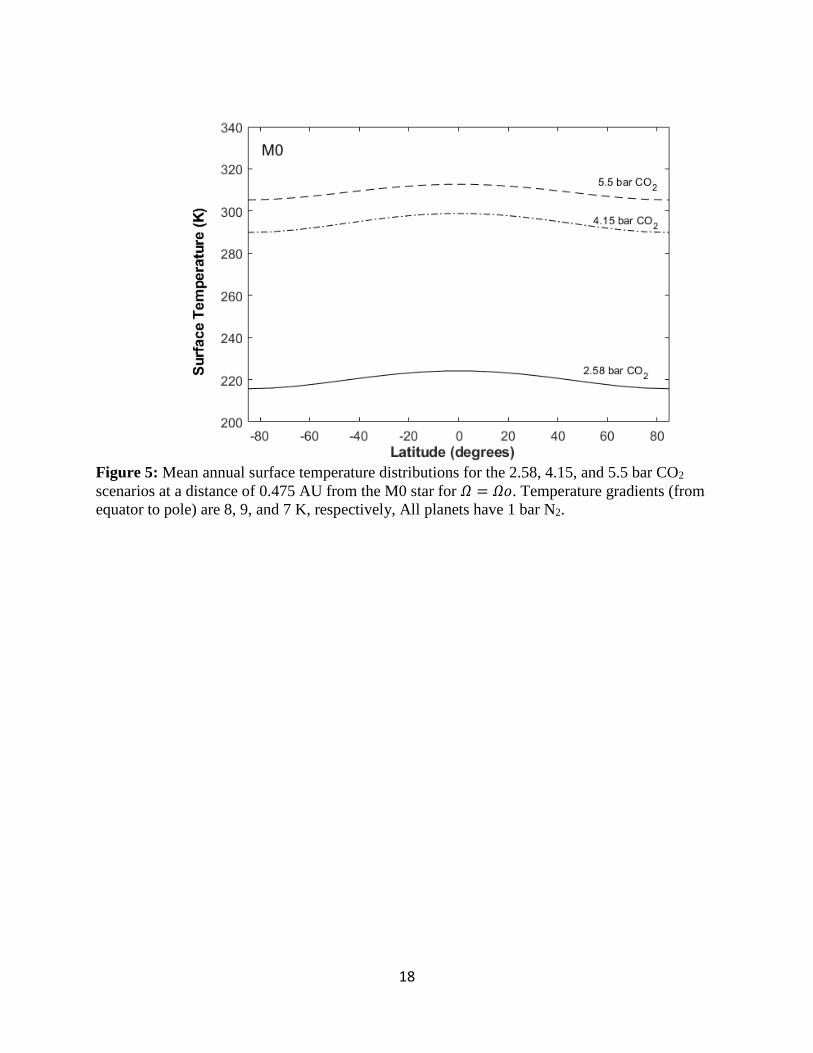
Figure 5: Mean annual surface temperature distributions for the 2.58, 4.15, and 5.5 bar CO2

scenarios at a distance of 0.475 AU from the M0 star for 𝛺 = 𝛺𝑜. Temperature gradients (from

equator to pole) are 8, 9, and 7 K, respectively, All planets have 1 bar N2.

19

Figure 6: Mean annual surface temperature distributions for the 200 micron case (4.15

bar CO2) at the inner edge for 𝛺 = a) 3𝛺𝑜 and b) 10𝛺𝑜.

20

Table 1: Inner edge boundaries (in AU) for different rotation rates (𝛺) and grain sizes (in

microns)

Stellar Class 3𝛺o 10𝛺𝑜

100 µ 200 µ 300 µ 100 µ 200 µ 300 µ

Sun 1.37 1.467 1.497 1.23 1.27 1.3

K2 0.79 0.832 0.865 0.69 0.705 0.714

M0 0.452 0.482 0.489 0.38 0.399 0.412

M3 0.256 0.268 0.277 0.219 0.226 0.236

M5 0.171 0.177 0.1837 0.146 0.15 0.158

M8 0.0502 0.053 0.055 0.0428 0.045 0.0461

5. DISCUSSION

5.1 EBM Critique and Justification

It is sometimes argued that the

diffusion parameterizations that many EBMs

use to describe equator-to-pole dynamic

transport (e.g., eq. 6) oversimplify

dynamical processes. Although this is a

common critique against EBMs, we believe

this argument is overstated because the

errors in these aspects are dwarfed by other

uncertainties regarding the exoplanets

themselves (including cloud cover, cloud

forcing, mass, atmospheric composition,

rotation rate etc.), which would be

problematic for any model to ascertain

without detailed observations. For example,

even though surface temperatures towards

higher latitudes across the tropics decrease

more rapidly in our EBM than what Earth

observations suggest, these differences are

relatively small (~1 to 3K) (Lindzen and

Farrell, 1977) (Fig. 7). Moreover, EBMs

tend to transition into an icy state somewhat

more abruptly than GCMs do (Shields et al.

(2013), but in spite of this, as our Fig. 7

shows, the northern hemispheric equator-

pole temperature gradients in the EBM are

similar to those observed for the Earth.

Although observations suggest that the

southern hemispheric pole is several degrees

colder than what our model would predict,

large topographic variations characterize

that hemisphere. However, topographic

features ought to be highly subdued on

planets whose outer condensed layer is a

global deep ocean, especially since the

maximum sea ice (enriched in CO2

clathrate) thickness is only ~2 m before

sinking (Levi et al. 2017). We note that the

best agreement between the EBM and Earth

occurs in the northern hemisphere, where

topographical variations are smallest

(Sellers, 1969). This suggests that our model

is appropriate for the flat and relatively

homogeneous ocean worlds we assess in this

study (as we argued in Section 3.3). In

comparison, the mean surface temperature

of the north pole in GCMs that lack ocean

heat transport is too cold by ~20 K (e.g

Shields et al. 2013). Our model also obtains

a mean surface temperature of 288 K and a

planetary albedo of ~0.3 for the Earth,

which gives further confidence in its

extrapolation to exoplanetary atmospheres.

Also, idealized GCM simulations

(lacking ocean heat transport and/or

employing simplified radiative transfer) of

the Earth predict that latitudinal temperature

gradients should increase at higher rotation

rates (e.g. Jenkins, 1993; Charnay et al.

2013; Kaspi and Showman, 2015), which is

broadly consistent with the diffusion

parameterization used in many advanced

21

EBMs (eq. 6). Although cloud behavior

changes with the rotation rate in those

models (whereas we keep our cloud

feedback constant), such results are

consistent with our analysis here. The latter

idealized GCM study showed that gradients

continually increased from an Earth-like

rotation rate to 8x that of Earth (Kaspi and

Showman, 2015). That said, we do not know

how well our diffusion parameterization

agrees with full atmospheric-ocean GCM

simulations at very high rotation rates for

these high-CO2 ocean world atmospheres.

However, we expect that such GCMs with

proper ocean heat transport should exhibit

even better agreement with EBM

simulations because ocean transport is

implicit in our diffusion parameterization. A

future study could assess this possibility.

Nevertheless, advanced EBMs

continue and will continue to be successfully

used for many planetary and exoplanetary

applications (e.g. North & Coakley (1979),

Williams and Kasting (1997), Caldeira &

Kasting (1992), Vladilo et al. (2013;2015),

Batalha et al. (2016); Forgan (2016), and

Haqq-Misra et al. (2016). They are

consistently able to obtain bulk trends that

are consistent with observations and

complex models in spite of their

simplifications. Our EBM is no different in

this regard. It is our hope that our study

motivates future GCM modelers to assess

how well predictions from such diffusion

parameterizations agree with fully-coupled

atmosphere-ocean model results in this high

rotation rate regime for thick CO2

atmospheres on ocean worlds. Such efforts

would yield improved parameterizations for

EBMs too. GCMs and simpler models

(EBMs and single-column climate models)

are both necessary to understand planetary

climates (Jenkins, 1993; Pierrehumbert et al.

2007).

Figure 7: Mean annual surface temperature as a function of latitude for the present Earth

comparing our model without topography and with topography against real observations. In the

model case with topography, surface temperatures were assumed to decrease with elevation

(zonally-averaged data from Sellers, 1969) at a characteristic lapse rate for the Earth (6.5 K/km).

22

5.2 Sensitivity Study: Weak Thermal Gradient

Approximation on Equator – Pole Gradients

The Levi et al. (2017) mechanism

operates under large equator-pole gradients.

We wrote our own version of the weak

thermal gradient (WTG) approximation (e.g.

Pierrehumbert, 2010) to assess whether such

large gradients may also be possible on

tidally-locked worlds. To clarify, the WTG

approximation only suggests that

temperature gradients within the free

atmosphere should be small, as expected for

tidally-locked planets (e.g. Mills and Abbot,

2013). However, surface temperature

gradients can still be quite large. We found

that equator-pole surface temperature

gradients in the most optically thin

(favorable) scenario (3.58 bar, including 1

bar N2) were only ~7 K, even assuming an

ocean wind speed (U) of 5 m/s, which is the

lowest considered by Levi et al. (2017).

Subsequently, these gradients are slightly

smaller than those computed by the EBM

for the Earth-rotation cases (Fig. 5). Surface

temperature gradients (ΔT) approaching

those necessary (> ~30 K) would only be

possible at U ~ < 1 m/s, which is

unrealistically low to support such large

surface temperature variations, especially

since U α 2/3T (Cullum et al. 2014). Thus,

this is consistent with our result that such

equator-pole temperature gradients cannot

be achieved if planets are not rotating rather

quickly, as we have argued throughout our

analysis.

5.3 Evidence of ice cap zone for observations

Our computed boundaries in Fig. 4

indicate that at least 3 currently confirmed

planets (Kepler 62-f, GL-581d, Kepler-

1229b), thought to be located in the classical

HZ, are also in our ice cap zone. Our ice cap

zone for M-stars is nominally valid for stars

hotter than ~3400 K (~M3) because planets

orbiting even cooler stars would likely be

tidally-locked (Leconte et al. (2015)

However, it is possible that planets orbiting

stars cooler than ~3400 K may experience a

brief period of rapid rotation post-accretion

before undergoing synchronous rotation.

During this brief period, these planets may

experience numerous freeze-thaw cycles,

depending on the time-scale for tidal

locking. If the latter is long enough, material

of biological interest may be produced.

The number of potentially habitable

ocean worlds should correspondingly

increase as upcoming missions, including

the James Webb Space Telescope (JWST)

and the Transiting Exoplanet Survey

Satellite (TESS), find many new targets

around low-mass stars. The C/O ratio is a

key atmospheric quantity that JWST would

infer from the atmospheric composition (e.g.

Greene et al., 2016). If we assume that other

greenhouse gas abundances are negligible

and CO2 is relatively well-mixed in the

atmosphere, then column abundances(N) of

CO2 and H2O (N = P/g) can be used to

readily derive the C/O ratio. For both edges

of the ice cap zone, these ratios are ~ 0.48 –

0.5, assuming a range of representative

mean surface temperatures: ~270 – 340 K

for the inner edge and 250 K for the outer

edge. All of our atmospheres are dominated

by CO2, resulting in a relatively narrow

range of predicted C/O ratios. Rotation

periods for exoplanets are difficult to

ascertain observationally. This work shows

that for ocean worlds located within the ice

cap zone, the atmospheric C/O ratio can

place an upper boundary on the rotation

period (Fig. 4).

Also, some ocean worlds may be

inferred directly from mass-radius

observations if they consist of enough water

by mass. For instance, a 2-Earth mass planet

with 50% water (by total mass) has a bulk

23

density of ~ 3 g/cm3, considerably lower

than for the Earth (~5.5 g/cm3) or Mars

(~3.9 g/cm3). Such planets would have low

atmospheric scale heights and observations

would easily distinguish them from planets

with massive H/He envelopes. Also, their

low bulk densities should be considerably

lower than those for CO2-rich terrestrial

planets with Earth-like water inventories

associated with the classical HZ. Therefore,

the bulk density is an initial filter, helping to

pinpoint ocean worlds within the ice cap

zone. The second filter would be the C/O

ratio helping to pinpoint those planets that

are more likely to be of biological interest.

5.4 The importance of rotation rate

Our results show that a different ice cap

zone can be defined as a function of the

planetary rotation rate and the assumed

particle size (Table I). Regardless of

rotation rate (10𝛺𝑜 𝑜𝑟 3.3𝛺𝑜 ), at least 3

confirmed planets are located within it (Fig.

4). Although our study is the first to show

the importance of rotation rate in CO2-rich

atmospheres near the outer edge of the

classical HZ, its importance has also been

demonstrated in studies of early Venus (e.g.

Yang et al. 2014; Way et al 2016). These

studies effectively suggest that the inner

edge of the classical HZ may move to

shorter distances if it is assumed that planets

can rotate much more slowly than the Earth.

5.5. Analysis of mechanism, caveats, and

future work

Our work here is meant to test the

viability of the Levi et al. (2017) mechanism

and to derive inner and outer edges for

potentially habitable ocean worlds around

various stars. We believe we have shown

that this hypothesis may be plausible for G2

– M3 stars although our mechanism does not

seem very plausible for stars cooler than

~3400 K.

We have provided limits for the ice cap

zone that are consistent with the atmospheric

conditions assumed. However, we note a

few caveats that could be assessed in future

work. The biggest uncertainty in these and

all other HZ calculations has arguably been

clouds. Clouds would conceivably affect the

latitudinal temperature-distribution relative

to our case in which we keep cloud coverage

constant. This could be studied in future

work. Although the relative importance of

clouds would very much depend on the

specific conditions of a given planet, future

work could assess different scenarios (e.g.

cloud coverage, distribution) and gauge their

effects on the boundaries. We also assumed

a fixed surface albedo for CO2 ice.

However, this would conceivably be a

function of local variables, including ice

thickness, atmospheric pressures, and

temperatures. Another big uncertainty is the

dynamics of sea-ice and how such ice near

the equator would operate at temperatures

near the freezing point of water. This would

affect the temperature below which global

glaciation ensues. However, sensitivity

studies (not shown) revealed that a threshold

temperature of 273 K instead of 265K would

only have a small effect on the outer edge

distance (~ 1%). A final uncertainty is the

ice-albedo feedback, which is parameterized

differently in different models (e.g. Curry et

al., 2001), and ours is no different in this

regard. Small differences in this may

slightly affect the computed inner and outer

edges. Given the uncertainties in all such

calculations, improved observations of

exoplanetary atmospheres would increase

our understanding and yield substantial

improvements to all (i.e. 1-D and 3-D)

exoplanet climate models.

24

6. CONCLUSION

We have found that a circumstellar region

around G-M stars in which the CO2 cycling

mechanism of Levi et al. (2017) operates on

ocean worlds could exist and that habitable

conditions may be possible for planets that

rotate at least ~ 3 times faster than the Earth.

These high rotation rates generate the

required equator-pole temperature gradients

necessary to sustain both cold subpolar and

warm subtropical regions in these dense (> ~

2.5 bar) CO2 atmospheres. This is important

for establishing freeze-thaw cycles, needed to

help life evolve in diluted ocean worlds. The

inner edge of this ice cap zone is moderately

dependent on ice grain size whereas the outer

edge is relatively insensitive to this

parameter. The widest ice cap zone,

assuming 100 micron ice Ih grains and a

rotation rate of ~2.4 hours, is ~1.23 - 1.65,

0.69 - 0.954, 0.38 – 0.528 AU, 0.219 – 0.308

AU, 0.146 - 0.206 AU, and 0.0428 - 0.0617

AU, for G2, K2, M0, M3, M5, and M8 stars,

respectively. However, unless the planets are

very young, we expect that planets orbiting

stars cooler than a ~ M3 will be tidally-locked

and so our mechanism would not apply to

such planets. This zone decreases in width at

larger ice Ih grain sizes and slower rotation

rates. We predict C/O ratios for our

atmospheres (~0.48 – 0.5) that can be verified

by future missions, including JWST.

ACKNOWLEDGEMENTS

We thank Mercedes Lopez-Morales and James F. Kasting for fruitful discussions regarding C/O

ratios and JWST observations. We also acknowledge helpful conservations with Lisa

Kaltenegger and Dimitar Sasselov. We also thank the anonymous referee for constructive

comments which improved our manuscript. Both R.M.R and A.L. acknowledge support by the

Simons Foundation (SCOL No. 290357, L.K.; SCOL No. 290360). R.M.R also acknowledges

support by the Carl Sagan Institute and the Earth-Life Science Institute.

25

REFERENCES

Abe, Yutaka, et al. "Habitable zone limits for dry planets." Astrobiology 11.5 (2011): 443-460.

Abbot, D. S., Cowan, N. B., & Ciesla, F. J. (2012). Indication of insensitivity of planetary

weathering behavior and habitable zone to surface land fraction. The Astrophysical

Journal, 756(2), 178.

Agol, E. (2011). Transit surveys for Earths in the habitable zones of white dwarfs. The

Astrophysical Journal Letters, 731(2), L31.

Alibert, Yann, and Willy Benz. "Formation and composition of planets around very low mass

stars." Astronomy & Astrophysics 598 (2017): L5.

Allard F., Guillot T., Ludwig H.-G., Hauschildt P. H., Schweitzer A., Alexander D. R., 2003, in

IAU Symp. 211, Brown Dwarfs,, ed. E. Mart’in (San Francisco, CA: ASP), 211, 325

Allard, F., F-Allard, N., Homeier, D., Kielkopf, J., McCaughrean, M.J., Spiegelman, F., 2007. K

H2 quasi-molecular absorption detected in the T-dwarf Inda Ba. A&A, 474, L21-24,

doi:10.1051/0004-6361:20078362

Allison, Ian, Richard Brandt, and Stephen Warren. 1993. "East Antarctic Sea Ice: Albedo,

Thickness Distribution, and Snow Cover ." Journal of Geophysical Research 98: 12417.

Attwater, James, Aniela Wochner, Vitor Pinheiro, Alan Coulson, and Philipp Holliger. 2010.

"Ice as a protocellular medium for RNA replication." NATURE COMMUNICATIONS 1: 76

Baranov YI, Lafferty W, Fraser G. 2004. Infrared spectrum of the continuum and dimer

absorption in the vicinity of the O2 vibrational fundamental in O2-CO2 mixtures.

Journal of molecular spectroscopy 228: 432-40

Batalha, Natasha E., et al. "Climate cycling on early Mars caused by the carbonate–silicate

cycle." Earth and Planetary Science Letters 455 (2016): 7-13.

Brandt, Richard, Stephen Warren, Anthony Worby, and Thomas Grenfell. 2005. "Surface

Albedo of the Antarctic Sea Ice Zone." Journal of Climate 18: 3606.

Briegleb, B. P., Minnis, P., Ramanathan, V., & Harrison, E. (1986). Comparison of regional

clear- sky albedos inferred from satellite observations and model computations. Journal of

Climate and Applied Meteorology, 25(2), 214-226

.

Caldeira, K., & Kasting, J. F. (1992). Susceptibility of the early Earth to irreversible glaciation

caused by carbon dioxide clouds. Nature, 359(6392), 226.

26

Charnay, Benjamin, et al. "Exploring the faint young Sun problem and the possible climates of

the Archean Earth with a 3‐D GCM." Journal of Geophysical Research: Atmospheres118.18

(2013).

Clarke, Andrew. "The thermal limits to life on Earth." International Journal of Astrobiology 13.2

(2014): 141-154.

Ćuk, M., & Stewart, S. T. (2012). Making the Moon from a fast-spinning Earth: a giant impact

followed by resonant despinning. science, 338(6110), 1047-1052.

Cullum, J., Stevens, D., & Joshi, M. (2014). The importance of planetary rotation period for

ocean heat transport. Astrobiology, 14(8), 645-650.

Curry, J. A., Schramm, J. L., Perovich, D. K., & Pinto, J. O. (2001). Applications of

SHEBA/FIRE data to evaluation of snow/ice albedo parameterizations. Journal of Geophysical

Research: Atmospheres, 106(D14), 15345-15355.

Fairén, A. G., Haqq-Misra, J. D., & McKay, C. P. (2012). Reduced albedo on early Mars does

not solve the climate paradox under a faint young Sun. Astronomy & Astrophysics, 540,

A13.

Farrell, Brian F. "Equable climate dynamics." Journal of the Atmospheric Sciences 47.24 (1990):

2986-2995.

Feistel, Rainer, and Wolfgang Wagner. 2006. "A New Equation of State for H2O Ice Ih."

Journal of Physical and Chemical Reference Data 35: 1021.

Forgan, Duncan. "Milankovitch cycles of terrestrial planets in binary star systems." Monthly

Notices of the Royal Astronomical Society 463.3 (2016): 2768-2780.

Genov, Georgi, Werner Kuhs, Doroteya Staykova, Evgeny Goreshnik, and Andrey Salamatin.

2004. "Experimental Studies on the Formation of Porous Gas Hydrates." American

Mineralogist 89: 1228-1239.

Gierasch, Peter J., and Owen B. Toon. "Atmospheric pressure variation and the climate of

Mars." Journal of the Atmospheric Sciences 30.8 (1973): 1502-1508.

Godolt, M., et al. "Assessing the habitability of planets with Earth-like atmospheres with 1D and

3D climate modeling." Astronomy & Astrophysics 592 (2016): A36.

Greene, T. P., Line, M. R., Montero, C., Fortney, J. J., Lustig-Yaeger, J., & Luther, K. (2016).

Characterizing transiting exoplanet atmospheres with JWST. The Astrophysical Journal, 817(1),

17.

Gruszka, M., & Borysow, A., 1997. Roto-Translational Collision-Induced Absorption of CO2for

27

the Atmosphere of Venus at Frequencies from 0 to 250 cm− 1, at Temperatures from 200

to 800 K. Icarus, 129(1), 172-177.

Gruszka, M., & Borysow, A., 1998. "Computer simulation of the far infrared collision induced

absorption spectra of gaseous CO2." Molecular physics 93.6: 1007-1016.

Haberle, R. M., McKay, C. P., Tyler, D., & Reynolds, R. T. (1996). Can synchronously rotating

planets support an atmosphere?. In Circumstellar Habitable Zones (p. 29). ed. by

Laurance R. Doyle, Travis House Publications (Menlo Park, California)

Haqq-Misra, J., Kopparapu, R. K., Batalha, N. E., Harman, C. E., & Kasting, J. F. (2016). Limit

cycles can reduce the width of the habitable zone. The Astrophysical Journal, 827(2),

120.

Jenkins, Gregory S. "A general circulation model study of the effects of faster rotation rate,

enhanced CO2 concentration, and reduced solar forcing: Implications for the faint young sun

paradox." Journal of Geophysical Research: Atmospheres98.D11 (1993): 20803-20811.

Joshi, M. M., and R. M. Haberle. "Suppression of the water ice and snow albedo feedback on

planets orbiting red dwarf stars and the subsequent widening of the habitable

zone." Astrobiology 12.1 (2012): 3-8.

Kanavarioti, Anastassia, Pierre-Alain Monnard, and David Deamer. 2001. "Eutectic Phases in

Ice Facilitate Nonenzymatic Nucleic Acid Synthesis." Astrobiology 1: 271.

Kaspi, Yohai, and Adam P. Showman. "Atmospheric dynamics of terrestrial exoplanets over a

wide range of orbital and atmospheric parameters." The Astrophysical Journal 804.1 (2015): 60.

Kasting, J. F. (1991). CO2 condensation and the climate of early Mars. icarus, 94(1), 1-13.

Kasting, J. F., Whitmire, D. P., & Reynolds, R. T. (1993). Habitable zones around main

sequence stars. Icarus, 101(1), 108-128.

Kasting, James F., et al. "Remote life-detection criteria, habitable zone boundaries, and the

frequency of Earth-like planets around M and late K stars." Proceedings of the National

Academy of Sciences 111.35 (2014): 12641-12646.

Kitzmann D., Alibert, Y., Godolt, M., Grenfell, J.L., Heng, K., Patzer, A.B.C., Rauer, H.,

Stracke, B., von Paris, P., 2015. "The unstable CO2 feedback cycle on ocean planets." MNRAS,

452, 3752

Kondrat'ev, K. Y. A. (1969). Albedo of the underlying surface and clouds. Radiation in the

Atmosphere (KYA Kondrat'ev)(Academic Press, New York) pp, 411-452.

Kopparapu, R. K., Ramirez, R., Kasting, J. F., Eymet, V., Robinson, T. D., Mahadevan, S., ... &

28

Deshpande, R. (2013). Habitable zones around main-sequence stars: new estimates.

The Astrophysical Journal, 765(2), 131.

Kopparapu, Ravi Kumar, et al. "Habitable zones around main-sequence stars: dependence on

planetary mass." The Astrophysical Journal Letters 787.2 (2014): L29.

Kuchner, M. J. 2003. Astrophysical J. Let 596: L105.

Kuhlbrodt T., Griesel A., MontoyaM., Levermann A., Hofmann M., Rahmstorf

S., 2007. "On the driving processes of the Atlantic meridional overturning circulation." Rev.

Geophys., 45, vol. 2

Leconte, Jérémy, et al. "Increased insolation threshold for runaway greenhouse processes on

Earth-like planets." Nature504.7479 (2013): 268-271.

Leconte, Jérémy, et al. "Asynchronous rotation of Earth-mass planets in the habitable zone of

lower-mass stars." Science347.6222 (2015): 632-635.

L ́eger, A, F Selsis, C Sotin, and al et. 2004. Icarus 169: 499.

Levi, Amit, Dimitar Sasselov, and Morris Podolak. 2014. "Structure and Dynamics of Cold

Water Super-Earths: the case of occluded CH4 and its outgassing." The Astrophysical

Journal 792: 125.

Levi, Amit, Dimitar Sasselov, and Morris Podolak. 2017. "The Abundance of Atmospheric CO2

in Ocean Exoplanets: a Novel CO2 Deposition Mechanism." The Astrophysical Journal

838 (1): 24.

Levy, Matthew, Stanley Miller, Karen Brinton, and Jeffrey Bada. 2000. "Prebiotic Synthesis of

Adenine and Amino Acids Under Europa-like Conditions." Icarus 145: 609-613.

Lindzen, Richard S., and Brian Farrell. "Some realistic modifications of simple climate

models." Journal of the Atmospheric Sciences 34.10 (1977): 1487-1501.

Luger, R, R Barnes, E Lopez, and al et. 2015. Astrobiology 15: 57.

Mardling, Rosemary A., and D. N. C. Lin. "Calculating the tidal, spin, and dynamical evolution

of extrasolar planetary systems." The Astrophysical Journal 573.2 (2002): 829.

Menor-Salvan, Cesar, Marta Ruiz-Bermejo, Marcelo Guzmμn, Susana Osuna-Esteban, and

Sabino Veintemillas-Verdaguer. 2009. "Synthesis of Pyrimidines and Triazines in Ice:

Implications for the Prebiotic Chemistry of Nucleobases ." Chemistry - A European

Journal 15: 4411-4418.

29

Mills, Sean M., and Dorian S. Abbot. "Utility of the Weak Temperature Gradient Approximation

for Earth-like Tidally Locked Exoplanets." The Astrophysical Journal Letters 774.2 (2013): L17.

Mutschler, Hannes, Aniela Wochner, and Philipp Holliger. 2015. "Freeze-thaw cycles as drivers

of complex ribozyme assembly ." Nat Chem. 7: 502–508.

North, G. R., & Coakley Jr, J. A. (1979). Differences between seasonal and mean annual energy

balance model calculations of climate and climate sensitivity. Journal of the

Atmospheric Sciences, 36(7), 1189-1204.

Paynter, D. J., & Ramaswamy, V. (2011). An assessment of recent water vapor continuum

measurements upon longwave and shortwave radiative transfer. Journal of Geophysical

Research: Atmospheres, 116(D20).

Perovich, Donald. 1990. "Evolution of sea ice optical properties during fall freeze-up." Edited by

W Spinrad. Ocean Optics X, Proceedings of the SPIE 1302: 520.

Perrin, M. Y., and J. M. Hartmann. "Temperature-dependent measurements and modeling of

absorption by CO2-N2 mixtures in the far line-wings of the 4.3 μm CO2 band." Journal of

Quantitative Spectroscopy and Radiative Transfer42.4 (1989): 311-317.

Pierrehumbert, R. T., Brogniez, H., and Roca, R.: On the Relative Humidity of the Atmosphere,

in: The Global Circulation of the Atmosphere, edited by: Schneider, T. and Sobel, A. H., 143–

185, Princeton Univ. Press, Princeton, NJ, USA, 2007.

Pierrehumbert, Raymond T. "A palette of climates for Gliese 581g." The Astrophysical Journal

Letters 726.1 (2010): L8.

Pierrehumbert, R., & Gaidos, E. (2011). Hydrogen greenhouse planets beyond the habitable

zone. The Astrophysical Journal Letters, 734(1), L13.

Ramirez, R. M., Kopparapu, R., Zugger, M. E., Robinson, T. D., Freedman, R., & Kasting, J. F.

(2014a). Warming early Mars with CO2 and H2. Nature Geoscience, 7(1), 59-63.

Ramirez, R. M., Kopparapu, R. K., Lindner, V., & Kasting, J. F. (2014b). Can increased

atmospheric CO2 levels trigger a runaway greenhouse?.Astrobiology, 14(8), 714-731.

Ramirez, R. M., & Kaltenegger, L. (2014). The habitable zones of pre-main-sequence stars. The

Astrophysical Journal Letters, 797(2), L25.

Ramirez, R. M., & Kaltenegger, L., 2016. Habitable Zones of Post-Main Sequence Stars. The

Astrophysical Journal, 823(1), 6.

Ramirez, R. M., & Kasting, J. F. (2017). Could cirrus clouds have warmed early

Mars?. Icarus, 281, 248-261.

30

Ramirez, R. M., & Kaltenegger, L. (2017). A volcanic hydrogen habitable zone. The

Astrophysical Journal Letters, 837(1), L4.

Ramirez, Ramses M. "A warmer and wetter solution for early Mars and the challenges with

transient warming." Icarus 297 (2017): 71-82.

Schwartz, Alan, and M Goverde. 1982. "Acceleration of HCN Oligomerization by Formaldehyde

and Related Compounds: Implications for Prebiotic Syntheses." Journal of Molecular

Evolution 18: 351-353.

Seager, Sara. "Exoplanet habitability." Science 340.6132 (2013): 577-581.

Sellers, William D. "A global climatic model based on the energy balance of the earth-

atmosphere system." Journal of Applied Meteorology 8.3 (1969): 392-400.

Shields, A. L., Meadows, V. S., Bitz, C. M., Pierrehumbert, R. T., Joshi, M. M., & Robinson, T.

D. (2013). The effect of host star spectral energy distribution and ice-albedo feedback on

the climate of extrasolar planets. Astrobiology, 13(8), 715-739.

Simpson, Fergus. "Bayesian evidence for the prevalence of waterworlds." Monthly Notices of the

Royal Astronomical Society 468.3 (2017): 2803-2815.

Slack, Glen. 1980. "Thermal conductivity of ice." Physical Review B 22: 3065 .

Tian, Feng, and Shigeru Ida. "Water contents of Earth-mass planets around M dwarfs." Nature

Geoscience 8.3 (2015): 177.

Vladilo, Giovanni, et al. "The habitable zone of Earth-like planets with different levels of

atmospheric pressure." The Astrophysical Journal 767.1 (2013): 65.

Vladilo, Giovanni, et al. "Modeling the surface temperature of Earth-like planets." The

Astrophysical Journal 804.1 (2015): 50.

Way, M. J., Del Genio, A. D., Kiang, N. Y., Sohl, L. E., Grinspoon, D. H., Aleinov, I., ... &

Clune, T. (2016). Was Venus the first habitable world of our solar system?. Geophysical

Research Letters, 43(16), 8376-8383.

Williams, D. M., & Kasting, J. F. (1997). Habitable planets with high obliquities. Icarus, 129(1),

254-267.

Wordsworth, R., F. Forget, and Vincent Eymet. "Infrared collision-induced and far-line

absorption in dense CO 2 atmospheres." Icarus 210.2 (2010): 992-997.

Wordsworth, Robin D., and Raymond T. Pierrehumbert. "Water loss from terrestrial planets with

CO2-rich atmospheres." The Astrophysical Journal 778.2 (2013): 154.

31

Wunsch, Carl, and Raffaele Ferrari. "Vertical mixing, energy, and the general circulation of the

oceans." Annu. Rev. Fluid Mech. 36 (2004): 281-314.

Yang, J., Boué, G., Fabrycky, D. C., & Abbot, D. S. (2014). Strong dependence of the inner edge

of the habitable zone on planetary rotation rate. The Astrophysical Journal Letters, 787(1), L2

Zsom, Andras, et al. "Toward the minimum inner edge distance of the habitable zone." The

Astrophysical Journal778.2 (2013): 109.

.