
The Ground State Energy of a Dilute Bose Gas in...
94
The Ground State Energy of a Dilute Bose Gas in Dimension n ≥ 3 PhD Dissertation by Anders Aaen January 14, 2014 Advisor: Søren Fournais Department of Mathematics Aarhus University
Transcript of The Ground State Energy of a Dilute Bose Gas in...

The Ground State Energy of a DiluteBose Gas in Dimension n ≥ 3
PhD Dissertation
by Anders AaenJanuary 14, 2014
Advisor: Søren FournaisDepartment of Mathematics
Aarhus University


Contents
1 Introduction 11.1 The Interacting Bose Gas . . . . . . . . . . . . . . . . . . . . . . . . . . 11.2 The Two-Body Problem . . . . . . . . . . . . . . . . . . . . . . . . . . . 31.3 Previous Works . . . . . . . . . . . . . . . . . . . . . . . . . . . . . . . . 51.4 Outline . . . . . . . . . . . . . . . . . . . . . . . . . . . . . . . . . . . . 81.A Proof of Theorem 1.2.2 . . . . . . . . . . . . . . . . . . . . . . . . . . . . 9
2 Momentum Space Representation 132.1 The Bogoliubov Approximation . . . . . . . . . . . . . . . . . . . . . . . 16
3 The Ground State Energy in Dimension n > 3 193.1 Introduction . . . . . . . . . . . . . . . . . . . . . . . . . . . . . . . . . . 193.2 The Leading Order Term . . . . . . . . . . . . . . . . . . . . . . . . . . 21
3.2.1 The Upper Bound . . . . . . . . . . . . . . . . . . . . . . . . . . 233.2.2 The Lower Bound . . . . . . . . . . . . . . . . . . . . . . . . . . 24
3.3 A Second Order Upper Bound . . . . . . . . . . . . . . . . . . . . . . . . 323.3.1 The Trial State . . . . . . . . . . . . . . . . . . . . . . . . . . . . 353.3.2 Computation of the Energy . . . . . . . . . . . . . . . . . . . . . 373.3.3 Estimates . . . . . . . . . . . . . . . . . . . . . . . . . . . . . . . 40
3.A Equivalence of Ensembles . . . . . . . . . . . . . . . . . . . . . . . . . . 443.B Dyson’s Upper Bound . . . . . . . . . . . . . . . . . . . . . . . . . . . . 47
4 The Second Order Upper Bound via Soft-Pair Fock States 534.1 Reduction to Small Torus . . . . . . . . . . . . . . . . . . . . . . . . . . 544.2 Construction of the Trial State . . . . . . . . . . . . . . . . . . . . . . . 564.3 The Pair-Hamiltonian . . . . . . . . . . . . . . . . . . . . . . . . . . . . 574.4 The Anti-Symmetric Interaction Terms . . . . . . . . . . . . . . . . . . . 67
4.4.1 Interaction with Three Non-zero Momenta . . . . . . . . . . . . . 674.4.2 Interactions with Four Non-zero Momenta . . . . . . . . . . . . . 71
4.5 Minimization and Estimates . . . . . . . . . . . . . . . . . . . . . . . . . 784.5.1 Dimension n = 3 . . . . . . . . . . . . . . . . . . . . . . . . . . . 794.5.2 Dimension n = 4 . . . . . . . . . . . . . . . . . . . . . . . . . . . 80
4.A Proof of Lemma 4.1.1 . . . . . . . . . . . . . . . . . . . . . . . . . . . . 814.B Proof of Lemma 4.1.2 . . . . . . . . . . . . . . . . . . . . . . . . . . . . 83
REFERENCES 84


Preface
The theory of quantum mechanics provides a mathematical model for describing inter-acting systems of microscopic particles. However, to do actual calculations with themodel can be a complicated matter, and many basic properties remain to be under-stood. A particular fundamental problem is the ground state energy of the interactingBose gas. Even this problem is, in its full generality, beyond reach of a mathematicaltreatment. If one considers a sufficiently dilute Bose gas, it is possible to do somethingthough. Using semi-rigorous methods, asymptotic low density formulas for the groundstate energy was derived by Bogoliubov in the 1940’s and by Lee, Huang and Yang inthe 1950’s. Subsequently many attempts were made to extract rigorous results fromtheir methods, but only with modest success. For a rather long period of time the sub-ject was quiescent. Now, starting with the experimental realization of Bose-Einsteincondensation in 1995, modern technology has shown it possible to test theoretical pre-dictions for Bose gasses in labs, which in turns has inspired a renewed interest in arigorous understanding of these important physical systems.
The present dissertation is the result of my Ph.D.-studies at the Department ofMathematics, Aarhus University. The aim of the project was to investigate the groundstate energy of a Bose gas in 4 spatial dimensions, motivated by a recent, but non-rigorous, calculation of Yang. I have succeeded to obtain rigorous results verifyingYang’s prediction to some precision (the leading order term), and almost consistentto higher precision (the correction term). It turned out that some of the rigorous3-dimensional methods may rather easily be applied in higher dimensions, while oth-ers cannot (at all?). I concluded the latter after having considered a somewhat newapproach, introduced by Yau and Yin, in 4 dimensions. Instead I was able to makea substantial simplification of their approach, and hence the title of my dissertationcontains also dimension n = 3.
There are several people I wish to thank. First and foremost I would like to thankmy advisor Professor Søren Fournais for his major commitment and patient guiding.I would also like to thank Professor Jan Philip Solovej for helpful discussions on thetopic in chapter 4. Part of the project was carried out while I was traveling aroundthe world, profiting from the Danish fellowship ’Rejselegat for Matematikere’. In thisregard, I would like to thank Professor Rod Gover at the Department of Mathematics,University of Auckland, and Professor Thomas Østergaard Sørensen at the Departmentof Mathematics, Ludwig Maximillians University, Munchen. I would like to thankMatthias Engelmann for proof-reading part of the manuscript. Finally, I thank my wife,Louisa, and our three children Marius, Elise and Bertram for your love and support.


Abstract
We consider a Bose gas in spatial dimension n ≥ 3 with a repulsive, radially symmetrictwo-body potential V . In the limit of low density ρ, the ground state energy per particlein the thermodynamic limit is shown to be (n − 2)|Sn−1|an−2ρ, where |Sn−1| denotesthe surface measure of the unit sphere in Rn, and a is the scattering length of V .Furthermore, for smooth and compactly supported two-body potentials, we derive anupper bound to the ground state energy with a correction term (1+γ)8π4a6ρ2| ln(a4ρ)|in 4 dimensions, where 0 < γ ≤ C‖V ‖1/2∞ ‖V ‖1/21 , and a correction term which is O(ρ2)in higher dimensions. Finally, we use a grand canonical construction to give a simplifiedproof of the second order upper bound to the Lee-Huang-Yang formula, a result firstobtained by Yau and Yin. We also test this method in 4 dimensions, but with a negativeoutcome.
Resume (Danish Abstract)
Vi betragter en Bose gas i rummelig dimension n ≥ 3 med et positivt, radialt sym-metrisk par-potential V . I grænsen af lav tæthed ρ vises det, at grundtilstandsenergienper partikel i den termodynamiske grænse er (n− 2)|Sn−1|an−2ρ, hvor |Sn−1| betegneroverflademalet af enhedssfæren i Rn, og hvor a er spredningslængden af V . Endvidere,for glatte par-potentialer med kompakt støtte udleder vi en øvre grænse til grundtil-standsenergien med et korrektionsled (1 + γ)8π4a6ρ2| ln(a4ρ)| i 4 dimensioner, hvor
0 < γ ≤ C‖V ‖1/2∞ ‖V ‖1/21 , og med et korrektionsled O(ρ2) i højere dimensioner. Endeliganvender vi en grand-kanonisk konstruktion til at give et simplificeret bevis for denøvre grænse til Lee-Huang-Yang formlen, et resultat først opnaet af Yau og Yin. Viafprøver ogsa metoden i 4 dimensioner, men med et negativt udfald.


Chapter 1
Introduction
In this chapter we introduce the model in consideration along with relevant basic con-cepts. We then discuss previous works by other people, and finally we give an outlineof our main results.
1.1 The Interacting Bose Gas
Consider the system of N identical particles in an n-dimensional cubic box Λ = ΛL =(−L/2, L/2)n of side length L. The starting point for a quantum mechanical descriptionof this system is the N -fold tensor product
HN := H⊗ · · · ⊗ H ∼= L2(ΛN ) (1.1.1)
of the single particle Hilbert space H = L2(Λ). We assume that the particles arebosons, meaning that we further restrict attention to the symmetric Hilbert space
HsymN∼= L2
sym(ΛN ),
consisting of all Ψ ∈ HN which are invariant under arbitrary permutations of the Ncoordinates. The possible states of the system are represented by the unit vectors inHsymN , and each physical observable in a state Ψ is given by the expectation value
〈A〉Ψ := 〈Ψ, AΨ〉
of a self-adjoint operator A on HsymN . The operator corresponding to the total energy
of the system is the Hamiltonian
HN,L =N∑i=1
− ~2
2m∆i + U(x1, . . . , xN ). (1.1.2)
Here ~ is the reduced Planck constant, m is the mass of a single particle and ∆i denotesthe Laplacian w.r.t. xi ∈ Rn. For simplicity we choose units so that ~2/(2m) = 1. Thesum in (1.1.2) models the total (non-relativistic) kinetic energy of the system, while
The Interacting Bose Gas
multiplication with U represents the interactions of the particles. We will assume apair-wise interaction, meaning that U has the form
U(x1, . . . , xN ) =∑
1≤j<k≤NV (xj − xk),
for some function V on Rn, usually called the two-body potential. Thus our Hamiltoniantakes the form
HN,L =
N∑i=1
−∆i +∑
1≤j<k≤NV (xj − xk). (1.1.3)
We always assume that V is nonnegative, radially symmetric and Borel measurable.To define HN,L more precisely, we consider the quadratic form
QN,L(Ψ) =
∫ΛN
( N∑i=1
|∇iΨ|2 +∑
1≤j<k≤NV (xj − xk)|Ψ|2
)dx1 . . . dxN
on L2sym(ΛN ) with appropriate boundary conditions. Usually these are either Dirichlet,
periodic or Neumann. That is, we consider QN,L on either of the domains
dom(QN,L
)= L2
sym(ΛN ) ∩
H1(ΛN ) (Neumann)
H1per(Λ
N ) (periodic)
H10 (ΛN ) (Dirichlet)
,
where H1per(Λ
N ) denotes the set of L-periodic functions in H1(ΛN ), and H10 (ΛN ) de-
notes the set of functions in H1(ΛN ) vanishing at the boundary of ΛN . In either caseQN,L is a closed quadratic form, and it is a well-known fact that the correspondinglinear map, which we denote by HN,L, is then a self-adjoint operator. The ground stateenergy of the Bose gas is the number
E0(N,L) := inf〈HN,L〉Ψ : ‖Ψ‖ = 1,
or equivalently, E0(N,L) is the lowest eigenvalue of HN,L. We are interested in thethermodynamic limit, meaning that we let N,L→∞ in a sequence with fixed densityN/Ln = ρ. Thus, the ground state energy per particle in the thermodynamic limit isthe quantity
e0(ρ) := limN→∞
E0(N, (N/ρ)1/n)
N,
defined for ρ > 0. This limit is well-understood, see e.g. [19]. In particular we willemploy the facts that e0(ρ) is a convex function of ρ and independent of boundaryconditions. To calculate e0(ρ) is one of the most fundamental problems in many-bodyquantum mechanics. Nevertheless, in its full generality, the problem is at the presentstage beyond reach! As we shall see below, there has been significant progress thoughin understanding the asymptotics of e0(ρ) in the dilute limit ρ → 0. In this limitthe ground state energy depends to some precision only on V via the solution to thetwo-body problem.
2

The Two-Body Problem
1.2 The Two-Body Problem
In dimension n ≥ 3 we letsn := (n− 2)|Sn−1|,
where |Sn−1| denotes the surface measure of the unit sphere in Rn. Then in particulars3 = 4π and s4 = 4π2.
Definition 1.2.1. Let n ≥ 3 and suppose that V is a nonnegative, radially symmetricand measurable function on Rn. The scattering length of V is the number a ≥ 0 givenby
snan−2 = inf
u
∫Rn|∇u|2 +
1
2V u2, (1.2.1)
where the infimum is taken over all nonnegative, radially symmetric functions u ∈H1
loc(Rn) satisfying u(r) → 1 as r → ∞. If the infimum is attained, we call theminimizer a scattering solution.
The scattering length in dimension n = 1, 2 can be defined using a local version of(1.2.1), see [11]. With the above definition, the scattering length has indeed dimensionof length, and hence
Y := anρ
is a dimensionless quantity. Notice also that a is finite if and only if V is integrableat infinity. Definition 1.2.1 above is motivated by the two-body problem in the limitL→∞. In fact, it is fairly easy to show the convergence
limL→∞
LnE0(2, L) = snan−2. (1.2.2)
From (1.2.2) we can give a simple heuristic argument for the ground state energy ofthe general problem. Since we are assuming particles to interact in pairs, we mightsuggest that the ground state energy of the N -body problem should be close to theground state energy of the two-body problem times the number of pairs. That is,
E0(N,L) ≈ N(N − 1)
2E0(2, L). (1.2.3)
Taking the thermodynamic limit and employing (1.2.2), we then obtain
e0(ρ) ≈ snan−2ρ. (1.2.4)
In fact, (1.2.4) turns out to be true, and we will prove it with rigorous upper and lowerbounds. We cannot help remark though, that in light of the complexity of the rigorousproof of (1.2.4), it may seem surprising that the above very simple heuristic argumentyields the correct answer! It should also be noted that the approximation (1.2.3) doesnot apply in dimension n = 2 (see e.g. [15]).
The general strategy for an upper bound to e0(ρ) is to construct a (trial) state withlow energy, and which is simple enough to do calculations with. Again, since we areconsidering a pair-wise interaction of the particles, we might suggest that a good trialstate to the general problem can be constructed from the scattering solution. Existence,uniqueness and other properties of the latter are established in the following theorem,which we prove in Appendix 1.A.
3

The Two-Body Problem
Theorem 1.2.2. Let n ≥ 3. If V ∈ L1(Rn) is nonnegative, radially symmetric andcompactly supported, then the infimum in (1.2.1) is a unique minimum, and the mini-mizer u satisfies the zero-energy scattering equation
−∆u+1
2V u = 0 (1.2.5)
in the sense of distributions on Rn. Moreover, u is continuous, radially symmetric,radially increasing and satisfies
u(r) ≥ 1− (a/r)n−2,
with equality for r ≥ R0, if supp(V ) ⊂ B(0, R0).
We will consider two alternative representations for the scattering length. Supposethat V satisfies the assumptions of Theorem 1.2.2. Let 1−w denote the correspondingscattering solution, and let
ϕ := V w and g = V − ϕ = V (1− w).
Then w can be represented as
w(x) =1
2Γ(g)(x) :=
1
2sn
∫Rn
g(y)
|x− y|n−2dy. (1.2.6)
Indeed, (w− Γ(g)/2) is a bounded, harmonic function on Rn and hence, by Liouville’stheorem, constant. In fact, since
|Γg(x)| ≤‖g‖L1(Rn)
sn · dist(x, supp g)n−2, x /∈ supp g,
we see that Γg(x)→ 0 as |x| → ∞. Since also w(x)→ 0 as |x| → ∞, the identity (1.2.6)follows. Now, for large |x|, we have w(x) = (a/|x|)n−2 by Theorem 1.2.2. Comparingwith (1.2.6) we see that
an−2 =1
2sn
∫Rn
(|x||x− y|
)n−2
g(y) dy,
for large |x|, and in the limit |x| → ∞, the dominated convergence theorem then yields
2snan−2 =
∫Rng(y) dy. (1.2.7)
Given any function f ∈ L1(Rn) we let
fp = f(p) :=
∫Rne−ip·xf(x) dx
denote its Fourier transform. Note that if f is real and even, then f is real. We alsonote that if f is radially symmetric, then so is f . The function w above is not inL1(Rn), since w(x) = (a/|x|)n−2 for large |x|. However, it follows from (1.2.5) that, as
4
Previous Works
a tempered distribution, w equals the function p 7→ gp/(2p2). We shall abuse notation
slightly by denoting
wp :=gp2p2
.
By (1.2.7) we have2sna
n−2 = g0 = V0 − ϕ0. (1.2.8)
Now notice that
ϕp =1
(2π)n
∫Vq−pwq dq =
1
(2π)n
∫Vq−p
gq2q2
dq
=1
(2π)n
∫Vq−pVq
2q2dq − 1
(2π)n
∫Vq−pϕq
2q2dq.
Using this iteratively and inserting into (1.2.8), we obtain the so-called Born series
2snan−2 = V0 −
1
(2π)3
∫V 2p
2p2dp+
1
(2π)6
∫ ∫VpVq−pVq
4p2q2dqdp− . . .
in terms of the Fourier transform of V .
1.3 Previous Works
The first systematic and semi-rigorous treatment of the 3-dimensional problem was byBogoliubov in the 1940’s [2] and Lee-Huang-Yang in the 1950’s [9, 10]. In particular thelatter used the so-called pseudo-potential method to derive the asymptotic expansion
e0(ρ) = 4πaρ
(1 +
128
15√πY 1/2 + o
(Y 1/2
))as Y → 0,
now known as the Lee-Huang-Yang formula (LHY). Subsequently several other deriva-tions of LHY appeared, but unfortunately none of them were rigorous [16]. The onlyrigorous result was the bounds
1
10√
2≤ e0(ρ)
4πaρ≤ 1 + CY 1/3 (Y sufficiently small)
obtained by Dyson in 1957 [3]. Here C > 0 is a constant independent of V . WhileDyson’s upper bound is consistent with the leading order term in LHY, the lower boundis off the mark by a factor 1/14. It took more than 40 years before a matching leadingorder lower bound was proved. This was done by Lieb-Yngvason [14], who showed that
e0(ρ) ≥ 4πaρ(1− CY 1/17
),
for Y sufficiently small, depending on V . Dyson actually only considered the hard-corepotential, but his upper bound was later generalized to nonnegative, radially symmetricpotentials [11]. Thus there is a rigorous proof of the leading order term in LHY:
5

Previous Works
Theorem 1.3.1 (Dyson/Lieb-Yngvason). Suppose that V is nonnegative, radially sym-metric, measurable and integrable at infinity. Then
e0(ρ) = 4πaρ[1 + o(1)
]as ρ→ 0.
The next problem is then to obtain a rigorous proof of the correction term in LHY.As we shall see below there has been success regarding an upper bound. However,for the matching lower bound there has only been limited progress. The method ofLieb-Yngvason has been improved by J.O. Lee and Yin in [8] to yield an error term oforder ρ1/3| ln ρ|3. Also, the result of Giuliani-Seiringer [6] shows that LHY is correctin a so-called simultaneously weak coupling and high density regime, and for a rathernarrow class of potentials. But the general problem remains open.
Unfortunately it is not easy to improve Dyson’s method directly. Instead it hasturned out successful to pass to momentum space (see Chapter 2). In [4] a trial stateof the form
Ψ = exp
(1
2
∑p 6=0
cpa+p a
+−p +
√N0a
+0
)|0〉 (1.3.1)
was used to derive the following upper bound:
Theorem 1.3.2 (Erdos-Schlein-Yau 2008). Suppose that V is nonnegative, radiallysymmetric and smooth with a decay V (x) ≤ C(1 + |x|)−(3+δ), for some δ > 0. Letλ > 0 be small and set V = λV . Then
e0(ρ) ≤ 4πaρ
(1 +
128
15√π
(1 + Cλ)Y 1/2
)+O(ρ2| ln ρ|) as ρ→ 0. (1.3.2)
Here a is the scattering length of V , while C > 0 is independent of V .
We see that the second order term in (1.3.2) has the correct order in Y , but the constantis only correct in the limit of weak coupling, λ → 0. The trial state (1.3.1) is inspiredby the Bogoliubov approximation (Section 2.1), and its crucial feature is that particlesof nonzero momenta appear only in pairs of opposite momenta p,−p. A similar statewas used by Girardeau and Arnowitt in [5] in the context of a Bose gas, only herethe energy was not evaluated explicitly. We also note that the approach in [4] has theadvantage over [5] that (1.3.1) is considered in a grand canonical ensemble. This is atechnical convenience which simplifies some of the calculations.
A trial state of the form (1.3.1) is in general believed to yield the energy of LHY,and the result of Theorem 1.3.2 above may at first sight appear to be close enough tothe desired to be repaired. This is not so easy though! In [4] the energy in the state Ψis calculated in terms of (integrals of various combinations of) the cp’s, and the task isthen to make the best possible choice of these coefficients. Unfortunately, this choiceis not obvious and a compromise must be taken. The strategy of [4] is to declare themain terms in consistency with the Bogoliubov approximation, and then a posteriorijustify that the neglected terms are indeed of lower order in the energy. Finally, theenergy of the main terms is calculated explicitly (in the dilute limit) and the result isthe right-hand-side of (1.3.2). It is an interesting question whether one could make abetter choice of the cp’s e.g. by taking some of the neglected terms in consideration
6

Previous Works
also. Nevertheless we want to point out the following: A trivial upper bound to e0(ρ)can be obtained by calculating the energy of the constant function,
e0(ρ) ≤ 1
2
(∫R3
V (x) dx
)ρ.
The integral here is the first term in the Born approximation to 8πa, and one can easilyshow that for a coupled potential V = λV , we then have
e0(ρ) ≤ 4πa(1 + Cλ)ρ.
The point is that, to get rid of the term Cλ, we clearly have to consider a more generaltrial state. This suggests that one really has to ’do more’ than (1.3.1) in order tocapture the correct constant in LHY. The challenge was taken up by Yau and Yin intheir paper [25] from 2009. They introduced a new type of trial state, extending theproperties of (1.3.1). More precisely, they include pairs with total momentum of orderρ1/2, the so-called soft-pair’s. This produces additional terms in the energy, and theirresult is an upper bound consistent with LHY:
Theorem 1.3.3 (Yau-Yin 2009). Suppose that V is nonnegative, radially symmetricand smooth with fast decay. Suppose furthermore that V is sufficiently small for theBorn series to converge. Then
lim supρ→0
(e0(ρ)− 4πaρ
(4πa)5/2ρ3/2
)≤ 16
15π2.
The proof of theorem 1.3.3 as it appears in [25] is severely complicated compared to theproof of Theorem 1.3.2 in [4]. The reason is mainly two-fold: Firstly, the trial state of[25] is more general, as it should be. Consequently there are more terms in the energyto be estimated, and some of the nice symmetry properties of (1.3.1) do not apply.Secondly, the trial state of [25] has a fixed number of particles, in contrast to [4].
Having discussed 3-dimensional results, we now turn briefly to other dimensions.The one-dimensional case with a delta-function potential was considered by Lieb-Linigerin [12] and turned out to be exactly solvable. In 2 dimensions the leading order termwas, to our knowledge, first identified by Schick [20] in 1971 to be 4πρ| lnY |−1. Thiswas rigorously proven to be correct by Lieb-Yngvason in 2001 [15]. To our knowledgethere are yet no rigorous results on the 2-dimensional correction term (in fact, it seemsthat there is not even complete consensus about what this term should be: compare e.g.[20], [24] and [17]). In [24] Yang reexamined the pseudo-potential method in dimension2, 4 and 5. In the latter he found the method inconclusive, while he in four dimensionsderived the expansion
e0(ρ) = 4π2a2ρ[1 + 2π2Y | lnY |+ o
(Y lnY
)]as Y → 0. (1.3.3)
We remark that in Yangs paper the correction 2π2Y | lnY | appears to be 4π2Y | lnY |,due to a minor miscalculation.
7

Outline
1.4 Outline
In Chapter 2 we describe in more detail some of the tools applied in the subsequentchapters. Also, we explain the Bogoliubov approximation and show how it leads toLHY. In particular this will motivate the ansatz in (1.3.1).
In Chapter 3 we consider the Bose gas in arbitrary dimension n > 3. We firstfollow the proofs of Dyson and Lieb-Yngvason and obtain n-dimensional upper andlower bounds to e0(ρ) (Theorem 3.2.2, Theorem 3.2.3 and Corollary 3.2.10). As aconsequence we get the following n-dimensional analogue of Theorem 1.3.1 above.
Theorem 1.4.1. Let n ≥ 3 and suppose that V is nonnegative, radially symmetric,measurable and decays faster than r−ν at infinity, where ν = (6n − 2)/5. Supposefurthermore that V admits a scattering solution. Then
e0(ρ) = snan−2ρ
[1 + o(1)
]as ρ→ 0.
Next we employ the trial state in (1.3.1) to obtain the following second order upperbounds.
Theorem 1.4.2. Let n ≥ 3 and suppose that V is nonnegative, radially symmetric,smooth and compactly supported with V (0) > 0. In dimension n = 4,
e0(ρ) ≤ 4π2a2ρ[1 + 2π2(1 + γ)Y | lnY |
]+O(ρ2) as ρ→ 0,
where 0 < γ ≤ C‖V ‖1/2∞ ‖V ‖1/21 . In dimension n ≥ 5,
e0(ρ) ≤ snan−2ρ+O(ρ2) as ρ→ 0.
The second order asymptotics of e0(ρ) becomes more subtle in dimension n > 3. Thecorrection to the energy is given in terms of certain integrals, which, in three dimensions,are exactly computable in the limit ρ → 0, in a straight-forward manner. This is notthe case in higher dimensions, and a more careful analysis has to be carried out. Indimension n ≥ 5 we have not even been able to identify the expansion parameter Yin the correction term, nor an explicit coefficient. Chapter 3 (except Appendix 3.B) issubmitted as a paper. We have included it here in its submitted form, and hence therewill be minor repetitions from Chapter 1 and Chapter 2.
In Chapter 4 we consider the Bose gas in dimension 3 and 4. We carry out a grandcanonical calculation of the energy in the Yau-Yin trial state from [25]. In 3 dimensionsthis yields a substantially simpler proof of the upper bound in Theorem 1.3.3 comparedto [25]. In fact, we show the following slightly stronger upper bound.
Theorem 1.4.3. Let n = 3 and suppose that V is nonnegative, radially symmetric,smooth and compactly supported with V (0) > 0. Let 0 < η < 1/52. Then
e0(ρ) ≤ 4πaρ
(1 +
128
15√πY 1/2
)+O
(ρ
32
+η)
as ρ→ 0.
In 4 dimensions, unfortunately, the method does not apply. We have included thecalculations though, and we will explain in detail the reason for this break down.
8

Proof of Theorem 1.2.2
1.A Proof of Theorem 1.2.2
The proof given here is a somewhat modified version of the one found in Appendix Ain [15]. Recall that n ≥ 3 and sn := (n−2)|Sn−1|. We start by noting that any radiallysymmetric function u ∈ H1
loc(Rn) is continuous away from the origin. Indeed if, say,r > r0 > 0, then, by the fundamental theorem of calculus,
|u(r)− u(r0)| ≤∫ r
r0
|u′(t)| dt ≤ 1
rn−10
∫ r
r0
|u′(t)|tn−1 dt (1.A.1)
=1
rn−10 |Sn−1|
∫r0≤|x|≤r
|∇u(x)| dx,
and the last quantity can be made arbitrarily small, by taking r sufficiently close to r0.Suppose that supp(V ) ⊂ B(0, R0) and fix and arbitrary R > R0. Let B = B(0, R)
and define the auxiliary functional E = ER by
E(u) =
∫B|∇u|2 +
1
2V |u|2
on the set D := u ∈ H1(B) : u = 1 on ∂B. Let E := infu∈D E(u). We claim thatE has a nonnegative, radially symmetric minimizer u ∈ D. To show this, choose aminimizing sequence uk ∈ D such that E(uk)→ E. In particular the sequence E(uk)is bounded and, since V is nonnegative, ∇uk is bounded in L2(B). Moreover, since(uk − 1) ∈ H1
0 (B), the Poincare inequality yields
‖uk‖L2(B) ≤ ‖uk − 1‖L2(B) + |B|1/2 ≤ C‖∇uk‖L2(B) + |B|1/2,
and hence uk is bounded in H1(B). By the Banach-Alaoglu theorem there exists au ∈ H1(B) and a subsequence, also denoted by uk, such that uk u weakly in H1(B).Since H1(B) is compactly embedded in L2(B), we may assume that uk → u in L2(B)and consequently also that uk → u a.e. Since D is a closed and convex subset of H1(B)it follows, by Mazur’s Theorem, that D is weakly closed and hence u ∈ D. Finally, byweak lower semicontinuity of the L2-norm and Fatou’s Lemma, we see that
E = lim infk→∞
E(uk) ≥ ‖∇u‖2L2(B) +1
2
∫B
lim infk→∞
V |uk|2 = E(u),
and hence u is a minimizer. Since |u| ∈ D and E(|u|) ≤ E(u), we may assume thatu is nonnegative. Moreover, we can assume that u is radial. To see this consider thefunction
us(x) :=
∫Sn−1
u(|x|ω) dµ(ω),
where µ denotes the normalized surface measure on Sn−1. By passing into polar coor-dinates it is evident that ‖us‖L2(B) ≤ ‖u‖L2(B) and∫
BV u2
s ≤∫BV u2.
9

Proof of Theorem 1.2.2
Moreover, an approximation argument employing the fact that D ∩ C1(B) is dense inD and that D is closed, shows that us ∈ D with
∇us(x) =
∫Sn−1
[∇u(|x|ω) · ω
] x|x|
dµ(ω), for x 6= 0. (1.A.2)
It follows that ‖∇us‖L2(B) ≤ ‖∇u‖L2(B), and hence E(us) ≤ E(u). We continue byestablishing further properties of u.
1. u is radially increasing. Suppose that 0 < s < t ≤ R and u(s) > u(t). Chooseτ ∈ (s, t] such that u(τ) ≤ u(r) for all r ∈ [s, t]. Then define the radial function
v(r) =
minu(τ), u(r) for 0 ≤ r ≤ τ
u(r) for r > τ.
Then v ∈ D and
E(u)− E(v) ≥ sn∫ τ
su′(r)2rn−1 dr > 0,
since otherwise u′ = 0 a.e. on [s, τ ] and consequently
u(τ)− u(s) =
∫ τ
su′(r) dr = 0.
However, E(v) < E(u) contradicts the fact that u is a minimizer.2. u is continuous. Since u is in H1(B) and is radial, it is continuous away from the
origin by the argument in (1.A.1). However, since u is increasing and bounded frombelow, it can be chosen to be continuous at the origin also.
3. u is the only nonnegative, radial minimizer. Suppose that also v is a nonnega-tive, radial minimizer (which by the above is continuous and radially increasing). Thefunction w :=
√u2 + v2 is in H1(B) with
∇w =
(u∇u+ v∇v)χE√
u2 + v2,
where E := x ∈ B : u(x)2 + v(x)2 > 0. A direct computation shows that∫B|∇w|2 +
∫E
|v∇u− u∇v|2
u2 + v2=
∫B|∇u|2 +
∫B|∇v|2
and, since (w/√
2) ∈ D and E(v) = E(u), it follows that
E(u) ≤ E(w/√
2) = E(u)− 1
2
∫E
|v∇u− u∇v|2
u2 + v2.
Consequentlyv∇u = u∇v a.e. on E. (1.A.3)
Fix 0 < ε < 1 and let A = x ∈ B : u(x) > ε. If A 6= B then A is an open annulus,since u is radially increasing and continuous. Now choose an arbitrary test functionϕ ∈ C∞0 (A), and let h = ϕ/u. Then h ∈ H1(A) with
∇h =(∇ϕ)u− ϕ∇u
u2.
10

Proof of Theorem 1.2.2
By (1.A.3) and an integration by parts (using that h vanishes on ∂A), we get∫Av∇h =
∫A
v
u∇ϕ−
∫Ah∇v =
∫A
v
u∇ϕ+
∫Av∇h,
and hence ∫A
v
u∇ϕ = 0. (1.A.4)
Since (1.A.4) holds for any ϕ ∈ C∞0 (A), it follows that v/u is constant on A, and theboundary conditions then yields u = v on A. We may take ε arbitrary small, so weconclude that u = v whenever u > 0. Finally, we of course also have u = v wheneverv > 0, and hence u = v.
4. u satisfies −∆u + 12V u = 0 in the sense of distributions on B. Notice that
V ∈ L1(B) by assumption, and hence V u is indeed a distribution. Fix an arbitraryv ∈ C∞0 (B). We need to show that∫
B−u∆v +
1
2V uv = 0. (1.A.5)
For each t ∈ R we have (u+ tv) ∈ D and
E(u+ tv) = E(u) + t2E(v) + t · Re
∫B∇u · ∇v +
1
2vuv
Since u minimizes E ,
0 =d
dtE(u+ tv)
∣∣t=0
= Re
∫B∇u · ∇v +
1
2V uv = Re
∫B−u∆v +
1
2V uv,
where the last equality follows from integration by parts and by noting that v (andderivatives of v) vanishes on ∂B. Replacing v with −iv we find that the imaginary partof the above integral vanishes and hence (1.A.5) holds.
5. Since u is radial and harmonic in R0 < |x| < R, and since u(R) = 1, it followsthat
u(r) = uas(r) :=1− (α/r)n−2
1− (α/R)n−2, R0 ≤ r ≤ R,
for some number α ≥ 0. Note that, in case α = 0, we have u = 1 on R0 ≤ |x| ≤ R,and hence u attains its maximum in an interior point of B(0, R). From the scatteringequation and the fact that V is nonnegative it follows that u is subharmonic, and henceu is constant. However, this implies that V = 0.
6. u(r) ≥ uas(r) for all 0 < r ≤ R. Suppose that u(ρ) < uas(ρ), for some 0 < ρ < R0.For ε > 0 we define
hε(r) = 2(u(r)− (1 + ε)uas(r)
), 0 < r ≤ R,
Notice that hε(r) = −2εuas(r), for r ≥ R0, and in particular hε(R) = −2ε. Also, hε isstrictly decreasing on [R0, R] (if V 6= 0) and hence hε(R0) > −2ε. By the particularchoice of
ε =uas(ρ)− u(ρ)
1− uas(ρ),
11

Proof of Theorem 1.2.2
we obtain hε(ρ) = −2ε. Now let Ω = x ∈ Rn : ρ < |x| < R. Since uas is harmonic, itfollows that hε is subharmonic on Ω and, by the maximum principle,
maxΩ
hε = max∂Ω
hε = −2ε,
which contradicts the fact that hε(R0) > −2ε.7. Employing 4. and 5., an integration by parts yields
E(u) = snαn−2[1− (α/R)n−2
]−1.
8. If R > R and u, u denotes the corresponding minimizers of ER and ER respec-tively, then
u(r) = u(R)u(r), for r ≤ R,
which in particular shows that α is independent of R. To verify this define
v(r) =
u(R)u(r), 0 ≤ r ≤ R
u(r), R < r ≤ R
SinceER(u) ≤ ER
(u/u(R)
)= u(R)−2ER(u),
we get
ER(v) = u(R)2ER(u) +
∫BR\BR
|∇u|2 +1
2V |u|2 ≤ ER(u)
and, by uniqueness, we must have v = u, as desired.To summarize: for each R > R0 we have a minimizer uR of the functional ER with
the properties 1.-8. We can easily obtain the desired minimizer u of the functional in(3.2.1). Simply let
u(r) =[1− (α/R)n−2
]uR(r) for r ≤ R,
where CR :=[1 − (α/R)n−2
]. By 8. u is well-defined. Fix an arbitrary nonnegative,
radial function v ∈ H1loc(Rn) satisfying v(r)→ 1 as r →∞. Since C−1
R u minimizes ER,we get
ER(u) = C2RER(uR) ≤ C2
RER(v/v(R)) = C2R/v(R)2ER(v),
and by taking the limit as R→∞, it follows that
snan−2 =
∫Rn|∇u|2 +
1
2V |u|2
On the other hand 7. implies that
ER(u) = C2RER(uR) = CRsnα
n−2,
and letting R→∞, we conclude that α = a. The remaining properties of u are easilyobtained from the corresponding properties of the minimizers of ER.
12

Chapter 2
Momentum Space Representation
In this chapter we describe the important idea of considering the Hamiltonian in mo-mentum space. It was this representation that led Bogoliubov to his famous approxi-mation, which we also explain here. In particular we will motivate the Lee-Huang-Yangformula and see how the Bogoliubov approximation leads to the ansatz in (1.3.1).
A standard trick in many-body quantum mechanics is to pass to the grand canonicalensemble. Thus we introduce the bosonic Fock (Hilbert) space
F = FL(H) :=∞⊕N=0
HsymN (Hsym
0 = H0 := C).
The special vector |0〉 := (1, 0, 0, . . .) is called the vacuum. Operators on N -particlespaces can then be lifted, or second quantized, to densely defined operators on the Fockspace by a componentwise action. We let
HL :=∞⊕N=0
HN,L (H0,L := 0) (2.0.1)
denote the second quantization of HN,L from (1.1.3). We furthermore let N = NLdenote the second quantization of multiplication with N on HN , i.e.
NΨ :=
∞⊕N=0
NΨN .
N is called the number operator on F . Now, the obvious question is how to retrieveinformation about e0(ρ) from this grand canonical setting. To answer this, we definethe ’grand canonical ground state energy’
EGC0 (N,L) := inf
〈HL〉Ψ : ‖Ψ‖ = 1, 〈N〉Ψ ≥ N
. (2.0.2)
Here 〈·〉Ψ := 〈Ψ, ·Ψ〉F denotes the expectation value w.r.t. the inner product of theFock space. In Appendix 3.A we prove the following result, provided Dirichlet boundaryconditions are imposed. Of course, since the statement in the lemma concerns only thethermodynamic limit, we expect it to hold for other boundary conditions as well.

CHAPTER 2. MOMENTUM SPACE REPRESENTATION
Lemma 2.0.1. Suppose that V ∈ L1(Rn) is nonnegative, radially symmetric and com-pactly supported. Suppose furthermore that V ≥ εχB(0,2R), for some ε,R > 0. Then
e(ρ) = limL→∞
EGC0 (ρLn, L)
ρLn.
We remark that Lemma 2.0.1 remains true if the condition 〈N〉Ψ ≥ N in (2.0.2) isreplaced by 〈N〉Ψ = N , which might appear more natural. The idea of the proof ofLemma 2.0.1 is to relate the canonical ground state energy to the grand canonicalground state energy via the Legendre transform. In order for the latter to be well-defined globally, we need high-density bounds on e0(ρ). It is at this point we need theassumption V ≥ εχB(0,2R). Of course, if V is continuous, then V (0) > 0 suffices, andhence this condition is imposed in the relevant theorems in the subsequent chapters.
Returning to the N -particle space in (1.1.1), we define the symmetrization Psym
initially on pure tensors in HN by
Psym(f1 ⊗ · · · ⊗ fN ) =1
N !
∑σ∈SN
fσ(1) ⊗ · · · ⊗ fσ(N),
where SN denotes the symmetric group of permutations of the numbers 1, . . . , N . ThenPsym extends to a bounded operator on HN in the usual way, and in fact it is anorthogonal projection. The symmetric space is then
HsymN = Psym(HN ).
Given any f ∈ H we define the creation operator a∗(f) : HN → HN+1 by
a∗(f)Ψ =√N + 1f ⊗Ψ.
The adjoint of a∗(f) is the operator a(f) : HN+1 → HN satisfying
〈Φ, a∗(f)Ψ〉 = 〈a(f)Φ,Ψ〉, for each Φ ∈ HN+1 and Ψ ∈ HN .
We call a(f) the annihilation operator. It easily follows that
a(f)(g ⊗Ψ) =√N + 1〈f, g〉Ψ
for any g ∈ H and Ψ ∈ HN . More importantly we define the bosonic creation andannihilation operators
asym(f) = a(f) and a∗sym(f) = Psyma∗(f)
on the symmetric spaces HsymN . We remark that a(f) automatically maps a symmetric
space into a symmetric space. This is not the case for a∗(f) and hence we need tocompose with the symmetrization. The bosonic creation an annihilation operators arealso the adjoint of one another and furthermore, they satisfy the canonical commutationrelations (CCR):[
asym(f), asym(g)]
= 0 =[a∗sym(f), a∗sym(g)
]and
[asym(f), a∗sym(g)
]= 〈f, g〉I,
14

CHAPTER 2. MOMENTUM SPACE REPRESENTATION
where [A,B] := AB − BA is the commutator of A with B, and where I denotes theidentity. We will apply the above general construction in a special setting. Let
Λ∗ = Λ∗L := (2π/L)Zn.
For each p ∈ Λ∗ we let up(x) = L−n/2eip·x, for x ∈ Rn. The set up : p ∈ Λ∗ is anorthonormal basis in H = L2(Λ). To keep notation simple we set
ap := asym(up) and a+p := a∗sym(up).
The CCR then takes the form
[ap, aq] = 0 = [a+p , a
+q ] and [ap, a
+q ] = δp,q.
Now, suppose that V, V ∈ L1(Rn) with a decay
|V (x)|+ |V (x)| ≤ C(1 + |x|)−(n+ε),
for some C, ε > 0. Then the L-periodization of V exists and the Poisson summationformula holds [7]:
VL(x) :=∑m∈Zn
V (x+mL) =1
Ln
∑p∈Λ∗L
Vpeip·x, x ∈ Rn. (2.0.3)
Note that
limL→∞
VL(x) =1
(2π)n
∫eip·xVp dp = V (x) (2.0.4)
by Fourier’s inversion formula. Suppose furthermore that V is nonnegative and radiallysymmetric. Then consider
HperN,L :=
N∑i=1
−∆i +∑
1≤j<k≤NVL(xj − xk) (2.0.5)
with periodic boundary conditions and let e0(ρ) denote the corresponding ground stateenergy per particle in the thermodynamic limit. Since V is nonnegative, it is clear thatV ≤ VL and consequently e0(ρ) ≤ e0(ρ). However, due to the convergence in (2.0.4),we expect that e0(ρ) = e0(ρ). With the periodic potential VL one can show that in thesense of quadratic forms [23],
HperN,L =
∑p
p2a+p ap +
1
2|Λ|∑p,q,r,s
p+q=r+s
Vp−ra+p a
+q aras, (2.0.6)
where all sums are over Λ∗, and where the original potential V reappears in terms ofits Fourier transform.
The creation and annihilation operators defined above do not preserve particle num-bers, e.g. ap maps from HN into HN−1. One particular advantage of passing to thegrand canonical ensemble is that the second quantization of the creation and anni-hilation operators (which we also denote by ap and a+
p ) are operators from F into
15
The Bogoliubov Approximation
itself. Moreover, a+p is still the (formal) adjoint of ap and the CCR, as well as the
representation (2.0.6), remain valid on a dense subset of F . Before we discuss the Bo-goliubov approximation we will illustrate how the grand canonical ground state of thenon-interacting system can be represented in terms of creation operators. Let
Ψ0 = exp(√
N0a+0
)|0〉 :=
∞∑m=0
(√N0a
+0 )m
m!|0〉. (2.0.7)
By employing the CCR it is easy to see that
〈Ψ0,Ψ0〉 = eN0 and 〈Ψ0,NΨ0〉 = N0.
Furthermore, it also clear that apΨ0 = 0, for each p 6= 0. Thus, if we take N0 = ρ|Λ|and then normalize, we have the grand canonical ground state of the non-interactingBose gas.
2.1 The Bogoliubov Approximation
The partially heuristic presentation given here follows [5, 16] rather closely. ConsiderH = Hper
L (the second quantization of (2.0.5)) on the set of normalized Fock states Ψwith an expected number of particles 〈N〉Ψ = N := ρ|Λ|. Bogoliubov’s way of thinkingof the dilute (and hence weakly interacting) Bose gas goes as follows: The ground stateof the noninteracting system is given in (2.0.7). In this state all particles are in thecondensate, i.e. have momentum zero. ’Turning on’ the weak interaction, still thevast majority of the particles are in the condensate, while a small amount of particlepairs with equal and opposite momenta are created from the condensate. Only fromparticle pairs, the other groups of particles, i.e. double pairs, triples and quartets, canbe created. Bogoliubov then proposes (the first ansatz) to discard all terms higherthan quadratic in ap and a+
p , for p 6= 0. Since the expected number of particles in the
condensate is given by the expectation of a+0 a0, Bogoliubov furthermore proposes (the
second ansatz) to replace the operators a0 and a+0 by
√N . The resulting operator is
HBog :=V0
2ρ(N − 1) +
∑p 6=0
(p2 + ρVp
)a+p ap +
1
2ρVp(αp + α+
p
),
where αp := apa−p. This operator can be diagonalized by a Bogoliubov transformationexp
(F), where
F =1
2
∑p6=0
γp(αp − α+
p
)and γ : Λ∗\0 → R is some even function to be chosen appropriately. Note that iF isself-adjoint, and hence exp
(F)
is unitary. We define the new ’creation and annihilationoperators’
bp := eFape−F and b+p = eFa+
p e−F .
Since exp(F)
is unitary, the bp’s also satisfy the CCR. Now, we claim that
bp = ap cosh γp + a+−p sinh γp. (2.1.1)
16

The Bogoliubov Approximation
To show this we introduce
ap(ε) := eεFape−εF , ε ∈ R.
Taking (formally) derivative w.r.t. ε we obtain
dapdε
(ε) = FeεFape−εF − eεFapFe−εF = [F (ε), ap(ε)],
where F (ε) := eεFFe−εF , and where we have also used that F commutes with eεF inthe last equality. We continue to calculate
[F (ε), ap(ε)] = eεF [F, ap]e−εF
=1
2eεF(γp[ap, α
+p ] + γ−p[ap, α
+−p])e−εF
= γpa+−p(ε),
where we have employed the commutator identity [A,BC] = [A,B]C + B[A,C], theCCR and γ−p = γp to obtain the last equality. Thus we have
dapdε
(ε) = γpa+−p(ε).
Since differentiation commutes with complex conjugation, it then follows that
d2apdε2
(ε) = γ2pap(ε).
The general solution to this ODE is
ap(ε) = Ap cosh(γpε) +Bp sinh(γpε),
and the boundary condition ap(0) = ap yields Ap = ap, while
γpa+−p = γpa
+−p(0) =
dapdε
(0) = γpBp.
This verifies (2.1.1). By choosing
tanh(2γp) =ρVp
p2 + ρVp,
it follows from a lengthy, but straight forward, calculation that
HBog = EBog0 +
∑p 6=0
(p4 + 2ρp2Vp
)1/2b+p bp,
where
EBog0 :=
V0
2ρ(N − 1) +
1
2
∑p 6=0
p2
[(1 +
2ρVpp2
)1/2
− 1− ρVpp2
].
17
The Bogoliubov Approximation
Since b+p bp is a nonnegative operator, it is now clear the (non-normalized) ground state
of HBog isΨBog = eFΨ0,
with Ψ0 given in (2.0.7), and the ground state energy is then simply EBog0 . In the
thermodynamic limit we have (replacing sums with integrals)
eBog0 (ρ) := lim
L→∞
EBog0
ρLn
=V0
2ρ+
1
2(2π)nρ
∫Rnp2
[(1 +
2ρVpp2
)1/2
− 1− ρVpp2
]dp
=1
2
V0 −
1
2(2π)n
∫V 2p
p2dp
ρ+Q(ρ), (2.1.2)
where
Q(ρ) :=1
2(2π)nρ
∫Rnp2
[(1 +
2ρVpp2
)1/2
− 1− ρVpp2
+ρ2V 2
p
2p4
]dp.
We recognize the terms in the curly brackets in (2.1.2) as the the first two terms inthe Born series (Section 1.2), which we denote by 8πa0 respectively 8πa1. Assumethat n = 3. By a change of variables p 7→ (V0ρ)1/2p and the dominated convergencetheorem, we find that
limρ→0
Q(ρ)
ρ3/2V5/2
0
=1
2(2π)3
∫R3
p2
[(1 +
2
p2
)1/2
− 1− 1
p2+
1
2p4
]dp =
1
2(8π)3/2
128
15√π,
and hence
Q(ρ) = 4πa0ρ128
15√π
(a3
0ρ)1/2
+ o(ρ3/2
)as ρ→ 0.
Thus we have shown the asymptotic formula
eBog0 (ρ) = 4π(a0 + a1)ρ+ 4πa0ρ
128
15√π
(a30ρ)1/2 + o
(ρ3/2
)as ρ→ 0.
Assuming that indeed eBog0 (ρ) ≈ e0(ρ) and replacing a0 + a1 respectively a0 with the
full scattering length a, we arrive at the Lee-Huang-Yang Formula. We end this chapterby remarking that, using the CCR, the Bogoliubov ground state above may be writtenin the form
ΨBog = exp
(1
2
∑p 6=0
cpa+p a
+−p +
√N0a
+0
)|0〉, (2.1.3)
where
cp :=1−
√1 + 2ρp−2Vp
1−√
1 + 2ρp−2Vp
.
In Section 3.3 we shall use the ansatz in (2.1.3), not a priori fixing the cp’s.
18
Chapter 3
The Ground State Energy inDimension n > 3
Abstract : We consider a Bose gas in spatial dimension n > 3 with a repulsive, radiallysymmetric two-body potential V . In the limit of low density ρ, the ground state energyper particle in the thermodynamic limit is shown to be (n−2)|Sn−1|an−2ρ, where |Sn−1|denotes the surface measure of the unit sphere in Rn and a is the scattering length ofV . Furthermore, for smooth and compactly supported two-body potentials, we deriveupper bounds to the ground state energy with a correction term (1+γ)8π4a6ρ2| ln(a4ρ)|in dimension n = 4, where 0 < γ ≤ C‖V ‖1/2∞ ‖V ‖1/21 , and a correction term which isO(ρ2) in higher dimensions.
3.1 Introduction
The experimental realization of Bose-Einstein Condensation in 1995 [1] has inspiredrenewed interest in a rigorous understanding of the interacting Bose gas, and in partic-ular the ground state energy. The typical model for the energy of N bosons enclosedin a box Λ = ΛL := (−L/2, L/2)n, is the Hamiltonian
HN,L =N∑i=1
−∆i +∑
1≤j<k≤NV (xj − xk) (3.1.1)
on L2sym(ΛN ) (the set of totally symmetric L2-functions on ΛN ). Here units are chosen
such that ~2/2m = 1, where m is the mass of a particle. We will always assume thatthe two-body potential V is a nonnegative and radially symmetric function on Rn. Let
E0(N,L) := inf σ(HN,L) = inf〈Ψ, HN,LΨ〉 : ‖Ψ‖ = 1
denote the ground state energy of the Bose gas, and let
e0(ρ) := limN→∞
E0(N, (N/ρ)1/n)
N(3.1.2)
denote the ground state energy per particle in the thermodynamic limit at densityρ > 0. The latter is independent of whatever boundary conditions imposed on Λ. We

Introduction
let a denote the scattering length of V (see section 3.2) and note that Y := anρ is adimensionless quantity.
In dimension n = 3, the asymptotic behavior of e0(ρ) in the limit of low densitywas studied by Bogoliubov [2], Lee-Yang [10] and Lee-Huang-Yang [9] in the 1940-50’s.In particular, the latter applied the pseudopotential method to derive the expansion
e0(ρ) = 4πaρ
(1 +
128
15√πY 1/2 + o
(Y 1/2
))as Y → 0,
now known as the Lee-Huang-Yang formula (LHY). To give a mathematical proof ofLHY is still an open problem, except in a special case of ρ in a so-called simultaneouslyweak coupling and high density regime, and for a rather narrow class of potentials[6]. Even to prove the leading order term in LHY turned out to be a hard problem:A variational calculation carried out by Dyson in 1957 [3] showed the upper bounde0(ρ) ≤ 4πaρ(1 + CY 1/3), for hard-core interactions. This has later been generalizedto general nonnegative, radially symmetric potentials [13]. However, no proof of amatching, leading order lower bound was available until 1998, where Lieb-Yngvasonmanaged to show that e0(ρ) ≥ 4πaρ(1 − CY 1/17). Their approach was improved in[8] to yield e0(ρ) ≥ 4πaρ(1 − Cρ1/3| ln ρ|3). At the present time, no lower bound hascaptured even the correct order in the expansion parameter Y in LHY. For the upperbound there has been success though: In [4] a trial state of the form
Ψ = exp
(1
2
∑p 6=0
cpa+p a
+−p +
√N0a
+0
)|0〉 (3.1.3)
was used to derive an upper bound
e0(ρ) ≤ 4πaρ
(1 +
128
15√π
(1 + Cλ)Y 1/2
)+ Cρ2| ln ρ|,
for a coupled two-body potential V = λV . While the correction term has the correctorder in Y , the constant is only correct in the limit of weak coupling, λ → 0. The(Fock) trial state (3.1.3) is inspired by the Bogoliubov approximation, and the crucialfeature is that particles of nonzero momenta appear only in pairs of opposite momenta.Similar states have previously been considered by Girardeau-Arnowitt [5] and Solovej[22] in the context of Bose gases. In a paper from 2009 [25] Yau-Yin introduced a newtrial state, extending the properties of (3.1.3). More precisely, they include pairs withtotal momentum of order ρ1/2 (however their trial state has a fixed number of particlesin contrast to (3.1.3)). This turns out to lower the energy significantly and their resultis an upper bound consistent with LHY. We note however that the calculation with theYau-Yin trial state is somewhat more involved than the computation with (3.1.3).
The model (3.1.1) has also been studied in other dimensions. The case n = 1 (witha delta-function potential) was already considered back in 1963 by Lieb-Liniger [12]and turned out to be exactly solvable. In two dimensions, the leading order term was,to our knowledge, first identified by Schick [20] in 1971 to be 4πρ| ln(a2ρ)|−1. This wasrigorously proven to be correct by Lieb-Yngvason in 2001 [15]. To our knowledge thereare yet no rigorous results on the 2-dimensional correction term (in fact, it seems that
20
The Leading Order Term
there is not even consensus about what this term should be: compare e.g. [20], [24]and [17]). In [24] Yang reexamined the pseudopotential method in dimension two, fourand five. In the latter he found the method inconclusive, while he in four dimensionsderived the expansion
e0(ρ) = 4π2a2ρ[1 + 2π2Y | lnY |+ o
(Y lnY
)]as Y → 0. (3.1.4)
We remark that in Yangs paper the correction 2π2Y | lnY | appears to be 4π2Y | lnY |,due to a minor miscalculation.
In this paper we test some of the rigorous 3-dimensional calculations in higherdimensions. We follow the proofs of Dyson and Lieb-Yngvason to obtain the n-dimensional upper- and lower bounds (Theorem 3.2.2 and Theorem 3.2.3),
1− CY α ≤ e0(ρ)
snan−2ρ≤ 1 + CY β, (3.1.5)
where sn := (n− 2)|Sn−1|, |Sn−1| denotes the surface measure of the unit sphere in Rnand where
α =n− 2
n(n+ 2) + 2and β =
n− 2
n.
Secondly, we employ the trial state (3.1.3) to improve the upper bounds. In dimensionn = 4 we show that (Theorem 3.3.1)
e0(ρ) ≤ 4π2a2ρ[1 + 2π2(1 + γ)Y | lnY |
]+ CV ρ
2,
where 0 < γ ≤ C‖V ‖1/2∞ ‖V ‖1/21 , consistent with (3.1.4) in the limit of weak coupling.In dimension n ≥ 5 the calculation yields the upper bound (Theorem 3.3.1)
e0(ρ) ≤ snan−2ρ+ Cρ2.
The second order asymptotics of e0(ρ) becomes more subtle in dimension n > 3. Thecorrection to the energy is given in terms of certain integrals, which, in three dimensions,are exactly computable in the limit ρ → 0, in a straight-forward manner. This is notthe case in higher dimensions, and a more careful analysis has to be carried out. Indimension n ≥ 5 we have not been able to identify the expansion parameter Y in thecorrection term, nor an explicit coefficient.
Finally, since (3.1.3) is a Fock state, we need the fact that the canonical ground stateenergy defined in (3.1.2) can be recovered from the grand-canonical setting. Althoughthis is a well-known result, we did not come across a good reference for it, and hencewe have included a proof in Appendix 3.A.
3.2 The Leading Order Term
In this section we prove the upper and lower bounds in (3.1.5). We will assume that Vis a nonnegative, radial and measurable function on Rn, where n ≥ 3. The scatteringlength of V is denoted by a and may be defined via the variational problem (see e.g.[11], [26])
snan−2 := inf
u
∫Rn|∇u|2 +
1
2V u2, (3.2.1)
21

The Leading Order Term
where the infimum is taken over all nonnegative, radially symmetric functions u ∈H1
loc(Rn) satisfying u(r) → 1 as r → ∞. Notice that such functions are automaticallycontinuous away from the origin. Also, it is easy to see that we may restrict attentionto radially increasing functions. Moreover, we remark that a is finite if and only if V isintegrable at infinity. In many cases the infimum in (3.2.1) is a unique minimum, andthe minimizer u satisfies the zero-energy scattering equation
−∆u+1
2V u = 0 (3.2.2)
in the sense of distributions on Rn. The existence of a scattering solution for a non-negative, radially symmetric and compactly supported potential is established in [15].We note briefly some properties of the scattering solution u, referring to [15], [11] fordetails:
(i) For large r, u(r) ≈ 1− (a/r)n−2, or more precisely
limr→∞
1− u(r)
(a/r)n−2= 1. (3.2.3)
In factu(r) ≥ 1− (a/r)n−2, (3.2.4)
with equality for r > R0 if supp(V ) ⊂ B(0, R0).
(ii) Monotonicity: If V ≤ V , then a ≤ a, while u ≥ u.
(iii) Regularity imposed on V is inherited by u. For instance, one may apply ellipticregularity and Sobolev imbedding’s to show that if V is smooth, so is u.
(iv) For V ∈ L1(Rn), it follows from (4.B.2) that u can be represented as
1− u(x) =1
2Γ(V u)(x) :=
1
2sn
∫Rn
V (y)u(y)
|x− y|n−2dy. (3.2.5)
By (3.2.3) and the dominated convergence theorem it then follows that
2snan−2 =
∫RnV (x)u(x) dx. (3.2.6)
The main result of this section is the following, which is an immediate consequenceof Theorem 3.2.2 and Corollary 3.2.10 below.
Theorem 3.2.1. Let n ≥ 3 and suppose that V is nonnegative, radially symmetric,measurable and decays faster than r−ν at infinity, where ν = (6n − 2)/5. Supposefurthermore that V admits a scattering solution. Then
limρ→0
e0(ρ)
snan−2ρ= 1. (3.2.7)
22

The Leading Order Term
3.2.1 The Upper Bound
We have the following dimensional generalization of [3], [11].
Theorem 3.2.2. Let n ≥ 3 and suppose that V is nonnegative, radially symmetric andmeasurable.
(i) Without further assumptions,
lim supρ→0
e0(ρ)
snan−2ρ≤ 1.
(ii) There exist C, δ > 0 independent of V such that, if V admits a scattering solution,then
e0(ρ) ≤ snan−2ρ[1 + CY 1−2/n
],
whenever Y ≤ δ.
Proof. We employ the periodic trial state of Dyson [3]. This state is not symmetric,but since the ground state of HN,L on the full space L2(ΛN ) is symmetric [11], weobtain an upper bound to e0(ρ). Suppose that u ∈ H1
loc(Rn) is nonnegative, radiallysymmetric, increasing and moreover that u(r) → 1 as r → ∞. The trial state is thendefined by
Ψ := F2 · F3 · · ·FN ,
where
Fi := min1≤j<i
[minm∈Z
f(xi − xj −mL)
]and
f(r) :=
u(r)u(b) 0 ≤ r ≤ b
1 r > b,
for some (large) b > 0 to be chosen. Following the calculation in [11] we obtain
e0(ρ) ≤Jρ+ 2
3(Kρ)2
(1− Iρ)2, (3.2.8)
where
I :=
∫(1− f(x)2) dx, K :=
∫f(x)|∇f(x)| dx
and
J :=
∫|∇f(x)|2 +
1
2V (x)f(x)2 dx.
It follows that
lim supρ→0
e0(ρ)ρ−1 ≤ J ≤ 1
u(b)2
∫|∇u(x)|2 +
1
2V (x)u(x)2 dx,
where we have used
f(r) ≤ u(r)
u(b)and f ′(r) ≤ u′(r)
u(b)
23

The Leading Order Term
in the latter inequality. In the limit b→∞ we get
lim supρ→0
e0(ρ)ρ−1 ≤∫|∇u(x)|2 +
1
2V (x)u(x)2 dx,
and minimizing over u yields (i), by definition of the scattering length.In case V admits a scattering solution, we apply the above construction with u being
this particular function. The bound (3.2.4) then allow us to estimate more explicitly.Indeed, we have f(r) ≥ [1− (a/r)n−2]+, and hence
I ≤ |Sn−1|(∫ a
0rn−1 dr +
∫ b
a2an−2r dr
)≤ |Sn−1|an−2b2.
Next,
J ≤ snan−2
u(b)2≤ sna
n−2
(1− (a/b)n−2)2,
provided b > a. Finally, using f(r) ≤ 1 and an integration by parts yields
K ≤ |Sn−1|∫ b
0f ′(r)rn−1 dr ≤ |Sn−1|
(bn−1 − (n− 1)
∫ b
0f(r)rn−2 dr
).
However, ∫ b
0f(r)rn−2 dr ≥
∫ b
a
[1− (a/r)n−2
]rn−2 dr
=bn−1
n− 1− an−2b+
n− 2
n− 1an−1 ≥ bn−1
n− 1− an−2b,
and hence K ≤ |Sn−1|(n− 1)an−2b. Now, by choosing b := (|Sn−1|ρ)−1/n, we have
(a/b)n−2 = |Sn−1|an−2b2ρ = Y β,
where Y := |Sn−1|Y and β := (n− 2)/n. In total we have
e0(ρ) ≤ snan−2ρ
[1
(1− Y β)4+
CY β
(1− Y β)2
]≤ snan−2ρ
(1 + CY β
),
provided Y is bounded away from 1.
3.2.2 The Lower Bound
In this section we prove an n-dimensional lower bound by following the steps in [14].The assumption of compact support in Theorem 3.2.3 below is relaxed in Corollary3.2.10.
Theorem 3.2.3. Let n ≥ 3 and suppose that V is nonnegative, radially symmetric,measurable and compactly supported with, say, supp(V ) ⊂ B(0, R0). There exist C, δ >0 independent of V such that
e0(ρ) ≥ snan−2ρ(1− CY α
),
24

The Leading Order Term
where
α :=n− 2
n(n+ 2) + 2, (3.2.9)
provided
Y ≤ minδ, (a/R0)
n−25α. (3.2.10)
In order to prove Theorem 3.2.3 we consider H = HN,L with Neumann boundaryconditions on Λ. The first step is to obtain an n - dimensional version of Dyson’slemma. In what follows we set
an := (n− 2)an−2.
Lemma 3.2.4 (Dyson’s Lemma). Suppose that U is a measurable, nonnegative andradially symmetric function on Rn, which satisfies
U(r) = 0, for r ≤ R0, and
∫ ∞0
U(r)rn−1 dr ≤ 1.
Let B ⊆ Rn be open and star shaped w.r.t. the origin. Then∫B|∇ϕ(x)|2 +
1
2V (x)|ϕ(x)|2 dx ≥ an
∫BU(x)|ϕ(x)|2 dx,
for each ϕ ∈ H1(B).
Proof. For any ω ∈ Sn−1 we let
R(ω) = supr ≥ 0 : sω ∈ B, for each 0 ≤ s ≤ r
denote the (possibly infinite) distance from the origin to the boundary of B in thedirection of ω. Since B is open and star shaped w.r.t. the origin, it follows that, forany r ≥ 0, rω ∈ B if and only if r < R(ω). By passing into polar coordinates, we thensee that it suffices to show that, for each fixed ω ∈ Sn−1,∫ R(ω)
0
(|f ′(r)|2 +
1
2V (r)|f(r)|2
)rn−1 dr ≥ an
∫ R(ω)
0U(r)|f(r)|2rn−1 dr, (3.2.11)
where f(r) := ϕ(rω) with |f ′(r)| ≤ |∇ϕ(rω)|. We may assume that R(ω) > R0, sinceotherwise the right hand side in (3.2.11) vanishes, and we claim that∫ R(ω)
0
(|f ′(r)|2 +
1
2V (r)|f(r)|2
)rn−1 dr ≥ an|f(R)|2, (3.2.12)
for each R0 < R < R(ω). Indeed, if f(R) 6= 0, then the function u given by u(x) =|f(|x|)/f(R)| for |x| ≤ R and u(x) = 1 for |x| > R is admissible in (3.2.1), and sinceV (r) = 0, for r > R, it follows that
snan−2 ≤ |S
n−1||f(R)|2
∫ R(ω)
0
(|f ′(r)|2 +
1
2V (r)|f(r)|2
)rn−1 dr.
Now (3.2.11) follows by multiplying both sides of (3.2.12) with U(R)Rn−1 and thenintegrating w.r.t. R.
25

The Leading Order Term
Corollary 3.2.5. Suppose that U satisfies the conditions of Lemma 3.2.4, and define
W :=N∑i=1
U ti, ti(x1, . . . , xN ) := minj 6=i|xi − xj |.
Then H ≥ anW .
Proof. Since V is nonnegative and radial,
N∑i=1
V (ti(~x)) ≤N∑i=1
∑j<i
V (xi − xj) +N∑i=1
∑j>i
V (xi − xj) = 2∑i<j
V (xi − xj),
for each ~x = (x1, . . . , xN ), and hence
H ≥N∑i=1
(−∆i +
1
2V ti
). (3.2.13)
We focus on the first term i = 1, and fix x2, . . . , xN ∈ Λ. For j 6= 1 define
Bj = x1 ∈ Λ : t1(~x) = |x1 − xj |.
Fix an arbitrary ψ ∈ H1(ΛN ). By a change of variables x1 7→ x1 + xj , and by notingthat (Bj − xj) is star shaped w.r.t. the origin (indeed convex), we may apply Dyson’slemma to obtain∫
Bj
|∇1ψ(~x)|2 +1
2V (ti(~x))|ψ(~x)|2 dx1 ≥ an
∫Bj
U(t1(~x))|ψ(~x)|2 dx1, (3.2.14)
for each j 6= 1. Moreover, since the Bj ’s cover Λ disjointly (a.e.), we conclude that(3.2.14) holds with Bj replaced by Λ. Then, by Fubini’s theorem,∫
ΛN|∇1ψ(~x)|2 +
1
2V (t1(~x))|ψ(~x)|2 d~x ≥ an
∫ΛN
U(t1(~x))|ψ(~x)|2 d~x.
We get analogous contributions from i = 2, . . . , N in (3.2.13), and upon adding them,we obtain the result.
We now combine Corollary 3.2.5 with Temple’s inequality [18] in a perturbativeapproach. The parameters R and ε appearing below will be chosen appropriately lateron.
Lemma 3.2.6. Let 0 < ε < 1 and R0 < R < L/2. Suppose that
G(N,L) := επ2L−2 − snan−2L−nN2 > 0.
ThenE0(N,L) ≥ N(N − 1)K(N,L),
where
K(N,L) :=sna
n−2
Ln(1− ε)
(1− 2R
L
)n(1− vn
Rn
Ln
)N−2(1− n(n− 2)an−2N
(Rn −Rn0 )G(N,L)
)Here vn denotes the measure of the unit ball in Rn.
26
The Leading Order Term
Proof. Suppose that U and W are as in Lemma 3.2.4 respectively Corollary 3.2.5.Together with the fact that V is nonnegative, we then have a lower bound
H = εH + (1− ε)H ≥ −ε∆ + (1− ε)anW =: H,
and consequentlyE0(N,L) ≥ E0(N,L) := inf σ(H). (3.2.15)
We estimate E0(N,L) by employing Temple’s inequality in the ground state of −ε∆(with Neumann Boundary conditions), which is the constant function ϕ0(x) ≡ |Λ|−N/2with corresponding eigenvalue zero. Given any operator A on L2(ΛN ) with domaincontaining ϕ0, we let 〈A〉 = 〈ϕ0, Aϕ0〉. Temple’s inequality and (3.2.15) yields
E0(N,L) ≥ 〈H〉 − 〈H2〉 − 〈H〉2
E1 − 〈H〉
= (1− ε)an〈W 〉 −(1− ε)2a2
n
(〈W 2〉 − 〈W 〉2
)E1 − (1− ε)an〈W 〉
,
provided 〈H〉 < E1, where E1 is the second lowest eigenvalue of H. Note however that,since W is nonnegative, we have H ≥ −ε∆, and hence E1 ≥ επ2/L2, which is thesecond lowest eigenvalue of −ε∆. We now choose the function U to be
U(r) :=
n(Rn −Rn0 )−1 for R0 < r < R
0 otherwise.
By discarding the term 〈W 〉2, replacing (1 − ε) by 1 in two appropriate places andemploying the fact that
〈W 2〉 ≤ n ·N(Rn −Rn0 )−1〈W 〉,
we obtain
E0(N,L) ≥ (1− ε)an〈W 〉[1− nanN
(Rn −Rn0 )(επ2/L2 − an〈W 〉
)], (3.2.16)
provided an〈W 〉 < επ2/L2. To estimate this further, we need upper and lower boundson 〈W 〉, and we claim that
|Sn−1|Ln
N(N − 1)(1− 2R/L
)n(1− vnRn/Ln
)N−2 ≤ 〈W 〉 ≤ |Sn−1|Ln
N(N − 1). (3.2.17)
This will conclude the proof of the lemma. For the upper bound in (3.2.17) we fixx1 ∈ Λ and notice that
(x2, . . . , xN ) ∈ ΛN−1 : R0 < t1(~x) < R
⊆
N⋃j=2
Fj ,
27
The Leading Order Term
where ~x = (x1, . . . , xN ) and Fj = ΛN−1, except that the j’th factor is replaced byB(x1, R)\B(x1, R0). It follows that∫
ΛN−1
U(t1(~x)) dx2 . . . dxN ≤n
Rn −Rn0
N∑j=2
|Fj | = |Sn−1|(N − 1)|Λ|N−2.
By integrating over x1 ∈ Λ and then adding the identical contributions from the in-tegrals of U(t2), . . . , U(tN ), we arrive at the upper bound in (3.2.17). To verify thelower bound, we let Λ′ ⊆ Λ denote the cube with same center as Λ but with side lengthL− 2R. Fix x1 ∈ Λ′ and notice that B(x1, R) ⊆ Λ. We then have
N⋃j=2
Ej ⊆
(x2, . . . , xN ) ∈ ΛN−1 : R0 < t1(~x) < R, (3.2.18)
whereEj = (Λ\B(x1, R))N−1
except again that the j’th factor is replaced by B(x1, R)\B(x1, R0). Since the Ej ’s arepairwise disjoint, (3.2.18) implies that∫
ΛN−1
U(t1(~x)) dx2 . . . dxN ≥n
Rn −Rn0
N∑j=2
|Ej | = |Sn−1|(N − 1)(|Λ| − vnRn)N−2,
and integrating over Λ ⊃ Λ′ 3 x1, we obtain∫ΛN
U(t1(~x)) d~x ≥ |Sn−1|(N − 1)(L− 2R)n(|Λ| − vnRn)N−2.
Again, by adding identical contributions from the integrals of U(t2), . . . , U(tN ), we haveproved (3.2.17) and with it the lemma.
Note that, for fixed ρ > 0,
G(ρLn, L) ≤ π2L−2 − snan−2ρ2Ln < 0,
for large L, so Lemma 3.2.6 may not immediately be applied to get estimates in thethermodynamic limit.
Lemma 3.2.7. The mapping N 7→ E0(N,L) is superadditive, i.e.,
E0(k +m,L) ≥ E0(k, L) + E0(m,L), for all k,m ∈ N.
Proof. Fix an arbitrary normalized ψ ∈ H1(Λk+m). Since V is nonnegative, it followsthat
〈ψ,Hψ〉 ≥∫
Λk+m
k∑i=1
|∇iψ|2 +∑
1≤i<j≤kV (xi − xj)|ψ|2 (3.2.19)
+
∫Λk+m
k+m∑i=k+1
|∇iψ|2 +∑
k+1≤i<j≤k+m
V (xi − xj)|ψ|2.
28
The Leading Order Term
Then, by Fubini’s theorem,∫Λk+m
k∑i=1
|∇iψ|2 +∑
1≤i<j≤kV (xi − xj)|ψ|2 ≥
∫Λm
(E0(k, L)
∫Λk|ψ|2
)= E0(k, L),
and similarly for the second term on the right-hand side in (3.2.19) .
Lemma 3.2.8. Suppose that L/l ∈ N. Then
E0(N,L) ≥M ·minN∑m=0
cmE0(m, l), (3.2.20)
where M := (L/l)n and where the minimum is over all tuples (c0, . . . , cN ) of numberscm ≥ 0 subject to the conditions
N∑m=0
cm = 1 andN∑m=0
mcm = N/M. (3.2.21)
Proof. We partition Λ into M disjoint boxes Λ1, . . . ,ΛM , each of side length l. Corre-spondingly we have a partition Ωβ of ΛN ,
Ωβ := Λβ1 × . . .× ΛβN , β = (β1, . . . , βN ), 1 ≤ βj ≤M,
and hence
〈ψ,Hψ〉 =∑β
∫Ωβ
N∑i=1
|∇iψ|2 +∑i<j
V (xi − xj)|ψ|2. (3.2.22)
Fix a β as above. By Fubini’s theorem, the integration regime Ωβ may be replacedby Λα1
1 × . . . × ΛαMM , for some multiindex α ∈ NM0 with length |α| = N . For each0 ≤ m ≤ N , we let M · cm denote the number of components of α equal to m. Byfollowing the proof of Lemma 3.2.7, we split the kinetic energy into appropriate terms,and discard interactions between particles in different boxes to obtain the lower bound∫
Ωβ
. . . ≥(∫
Ωβ
|ψ|2) M∑j=1
E0(αj , l)
=
(∫Ωβ
|ψ|2)M
N∑m=0
cmE0(m, l)
≥(∫
Ωβ
|ψ|2)M min
( N∑m=0
cmE0(m, l)
).
Employing this estimate in (3.2.22) yields the result.
Lemma 3.2.9. Let ρ = N/Ln. Suppose that L/l ∈ N, R0 < R < l/2 and G(4ρln, l) >0. Then
E0(N,L)
N≥ (ρln − 1)K(4ρln, l).
29

The Leading Order Term
Proof. Suppose that cm ≥ 0 satisfies (3.2.21). We split the sum in (3.2.20) into twoparts: ∑
m
cmE0(m, l) =∑m<p
cmE0(m, l) +∑m≥p
cmE0(m, l), (3.2.23)
for some p ∈ N to be chosen. Suppose for now that G(p, l) > 0. Since G(N,L) andK(N,L) are decreasing functions of N , Lemma 3.2.6 implies that
E0(m, l) ≥ m(m− 1)K(p, l), for 0 ≤ m ≤ p, (3.2.24)
and hence ∑m<p
cmE0(m, l) ≥ K(p, l)∑m<p
cmm(m− 1).
Let t :=∑
m<pmcm. By the Cauchy-Schwarz inequality,
t2 ≤
(∑m<p
m2cm
)(∑m<p
cm
)≤∑m<p
m2cm,
and it follows that ∑m<p
cmm(m− 1) ≥ t(t− 1).
Thus we have ∑m<p
cmE0(m, l) ≥ K(p, l)t(t− 1).
We now employ the superadditivity of m 7→ E0(m, l) (Lemma 3.2.7) to obtain a lowerbound on the second sum on the right hand side in (3.2.23). For m ≥ p we writem = bm/pcp+ r, where bm/pc denotes the lower integer part of m/p and r ∈ N0 is theremainder. Notice that bm/pc ≥ m/(2p) always. The superadditivity of E0(m, l) thenyields
E0(m, l) ≥ m/(2p)E0(p, l),
and it follows that∑m≥p
cmE0(m, l) ≥ E0(p, l)
2p(k − t) ≥ 1
2(p− 1)(k − t)K(p, l),
where k := N/M = ρln. Altogether we have
N∑m=0
cmE0(m, l) ≥ K(p, l)[t(t− 1) +
1
2(p− 1)(k − t)
].
The choice p = b4kc implies that x 7→(x(x − 1) + 1
2(p − 1)(k − x))
is decreasing on[0, k], which is where t lies, and hence the minimum is taken at x = k. Thus we havethat
E0(N,L)
N≥ 1
ρln
∑m
cmE0(m, l) ≥ K(p, l)(k − 1),
as claimed.
30
The Leading Order Term
We can now finish the proof of Theorem 3.2.3.
Proof of Theorem 3.2.3. Suppose that the conditions of Lemma 3.2.9 are satisfied. Re-call that Y = anρ. Then
E0(N,L)
N≥ sna
n−2ρ(1− ε
)(1− 2nR/l
)[1− Y −1(a/l)n
]×
[1− 4vnY (l/a)n(R/l)n
][1− 4n(n− 2)lnY
(Rn −Rn0 )(επ2(a/l)2 − 16snY 2(l/a)n)
].
We now make the ansatz
ε = Y α, a/l = Y β,Rn −Rn0
ln= Y γ ,
for exponents α, β, γ > 0. In particular this implies that(R
l
)n= Y γ +
(R0
a
)nY nβ ≤ 2Y γ ,
provided
Y ≤(a
R0
)n/(nβ−γ)
. (3.2.25)
Thus we have
E0(N,L)
N≥ sna
n−2ρ(1− Y α
)(1− C1Y
γ/n)(
1− Y nβ−1)(
1− C2Y1+γ−nβ)
×(
1− C3Y1−α−2β−γ
1− C4Y 2−α−(n+2)β
).
In attempt to fit exponents we choose β and γ such that
γ/n = α = nβ − 1,
which in particular implies that 1 + γ − nβ = 2α. Now, the optimal choice of α, suchthat
1− α− 2β − γ ≥ α and 2− α− (n+ 2)β > 0,
is given in (3.2.9). With this choice the requirements of Lemma 3.2.9 are indeed satisfiedif Y is sufficiently small (depending only on the dimension) and if we take L = kl, foran integer k ∈ N. Also (3.2.25) is exactly the latter condition in (3.2.10). By lettingk →∞ we therefore conclude the proof.
Corollary 3.2.10. Suppose that V is nonnegative, radial and measurable with a decayV (r) ≤ Cr−ν , for large r, where ν > (6n − 2)/5. Suppose furthermore that V admitsa scattering solution. There exist a constant C > 0 depending only on n and a δ > 0depending on n, V such that
e0(ρ) ≥ snan−2ρ(1− CY α
),
provided Y ≤ δ.
31

A Second Order Upper Bound
Proof. Let R > 0 and define VR = V χB(0,R) with scattering length aR ≤ a. Since Vis nonnegative, replacing V with VR cannot increase the energy. By Theorem 3.2.3 wethen have
e0(ρ) ≥ snan−2R ρ
(1− CY α
R
)≥ snan−2
R ρ(1− CY α
),
provided YR := anRρ is sufficiently small and
YR ≤(aRR
)n−25α
. (3.2.26)
Denote the scattering solutions of V and VR by u respectively uR. Then, by (3.2.6),
an−2 − an−2R =
1
2sn
∫V (x)u(x)− VR(x)uR(x) dx
≤ 1
2sn
∫V (x)− VR(x) dx =
1
2sn
∫|x|≥R
V (x) dx,
where the inequality follows from the fact that u ≤ uR ≤ 1. From the decay of V weobtain
an−2R ≥ an−2
(1− K
2(n− 2)an−2Rε
),
provided R is sufficiently large. By choosing R such that
K
2(n− 2)an−2Rε= Y α,
it follows that R is large,an−2R ≥ an−2
(1− Y α
),
and (3.2.26) is satisfied, if Y is sufficiently small and ν > (6n− 2)/5.
3.3 A Second Order Upper Bound
In this section we derive a second order upper bound to e0(ρ) by estimating the energyin the state (3.1.3). The calculation is inspired by [4].
Theorem 3.3.1. Let n ≥ 3 and suppose that V ∈ C∞0 (Rn) is nonnegative and radiallysymmetric with V (0) > 0. There exist δ, C > 0 (depending on n, V ) such that
e0(ρ) ≤ snan−2ρ[1 + (1 + γ)Qn
]+ CΩn, (3.3.1)
provided ρ ≤ δ, where
Q3 =128
15√πY 1/2 Ω3 = ρ2| ln ρ|
Q4 = 2π2Y | lnY | Ω4 = ρ2
Qn = Cρ Ωn = ρ2, n ≥ 5
and 0 < γ ≤ C ′‖V ‖1−2/n∞ ‖V ‖2/n1 . Here C ′ > 0 depends only on n.
32

A Second Order Upper Bound
The assumptions on V in Theorem 3.3.1 are presumably not optimal. In the actualgrand-canonical calculation below, we only need V and its Fourier transform to decaysufficiently fast at infinity (depending on the dimension), and of course the latter can bemet by imposing finite smoothness on V . We use compact support of V and V (0) > 0in Lemma 3.3.2 below, which allows us to relate the canonical- and ’grand canonical’ground state energies. Presumably the assumption of compact support can be relaxedto a sufficiently fast decay.
In order to prove Theorem 3.3.1 we initially consider (3.1.1) with Dirichlet boundaryconditions. Our calculation below is carried out in the grand canonical ensemble, andhence we consider the second quantization of HN,L
HL :=∞⊕N=0
HN,L on FL :=∞⊕N=0
L2sym(ΛNL ), (3.3.2)
with the corresponding ’grand canonical ground state energy’
EGC0 (N,L) := inf
〈HL〉Ψ : ‖Ψ‖F = 1, 〈N〉Ψ ≥ N
, (3.3.3)
where N = NL denotes the number operator on FL and 〈A〉Ψ denotes the expectation〈Ψ, AΨ〉 of any operator A with Ψ in its domain. Consider the canonical and grandcanonical ground state energy per volume,
eL(ρ) :=E0(ρLn, L)
Ln, eGC
L (ρ) :=EGC
0 (ρLn, L)
Ln. (3.3.4)
We will assume that the limit
e(ρ) := limL→∞
eL(ρ) (3.3.5)
is a convex function of ρ (see e.g. [19]). The following result, which we prove in appendix3.A, shows that, in the thermodynamic limit, the canonical and grand canonical energiesagree.
Lemma 3.3.2. Suppose that V ∈ L1(Rn) is nonnegative, radially symmetric and com-pactly supported. Suppose furthermore that V ≥ εχB(0,2R), for some ε,R > 0. Then
e(ρ) = limL→∞
eGCL (ρ).
By (3.3.3) it is clear that ρ 7→ eGCL (ρ) is increasing, for any fixed L. As a consequence
we have the following slightly stronger result.
Corollary 3.3.3. Suppose that V satisfies the assumptions of Lemma 3.3.2, and sup-pose that ρL → ρ as L→∞. Then
e(ρ) = limL→∞
eGCL (ρL)
33

A Second Order Upper Bound
Proof. Fix an arbitrary ε > 0. By assumption e(ρ) is convex and hence continuous.Thus we can choose δ > 0 such that
|e(ρ)− e(ρ′)| ≤ ε,
for each ρ′ > 0 with |ρ− ρ′| ≤ δ. Then, for L sufficiently large,
eGCL (ρL) ≥ eGC
L (ρ− δ)=
[eGCL (ρ− δ)− e(ρ− δ)
]+ e(ρ− δ)
≥[eGCL (ρ− δ)− e(ρ− δ)
]+ e(ρ)− ε.
By Lemma 3.3.2 it then follows that
lim infL→∞
eGCL (ρL) ≥ e(ρ)− ε.
Similarly we can show a consistent upper bound, and since ε was arbitrary, the resultfollows.
In Section 3.3.1 we construct a periodic trial state with an expected number ofparticles 〈N〉 = ρLn, not directly leading to an upper bound on e0(ρ) via Lemma 3.3.2.However, Lemma 3.3.4 below, which is essentially proved in [25], shows that given anyperiodic state, we can find a Dirichlet state on a slightly larger box, with almost as lowenergy. We let
VL(x) :=∑m∈Zn
V (x+mL) =1
Ln
∑p∈Λ∗L
Vpeip·x, x ∈ Rn
denote the L-periodization of V , where Λ∗L := (2π/L)Zn and
Vp :=
∫Rne−ip·xV (x) dx
denotes the Fourier transform of V , which is real-valued and radially symmetric, sinceV is. Then let
HN,L :=N∑i=1
−∆i +∑
1≤j<k≤NVL(xj − xk)
with periodic boundary conditions, and let HL denote its second quantization. Notethat, since V is nonnegative, it is clear that V ≤ VL, and hence the transition from Vto VL cannot decrease the energy. However, since VL → V pointwise as L → ∞, weexpect the ground state energy of the two systems to coincide in the thermodynamiclimit.
Lemma 3.3.4. Let L > 2l > 0. Then
EGC0 (N,L+ 2l) ≤ 〈HL〉Ψ + C
N
lL,
for each periodic, normalized Ψ ∈ FL with 〈N〉Ψ = N . Here C > 0 depends only on n.
34

A Second Order Upper Bound
We apply Lemma 3.3.4 with l :=√L/2 and notice that
EGC0 (ρLn, L+ 2l)
ρLn=EGC
0 (ρL+2l(L+ 2l)n, L+ 2l)
ρL+2l(L+ 2l)n,
where
ρL :=ρ(L− 2l)n
Ln→ ρ as L→∞.
Together with Corollary 3.3.3 we conclude that
e0(ρ) ≤ lim supL→∞
〈HL〉ΨρLn
,
for each periodic, normalized Ψ ∈ FL with expected number of particles 〈N〉Ψ = ρLn.Finally, we note that, with the periodic potential VL, we have (in the sense of
quadratic forms)
HL =∑p
p2a+p ap +
1
2Ln
∑p, q, r, s
p+ q = r + s
Vp−ra+p a
+q aras, (3.3.6)
where all sums are over Λ∗L and where a+p and ap denote the bosonic creation and
annihilation operators on FL w.r.t. the plane wave x 7→ L−n/2eip·x.
3.3.1 The Trial State
The state in (3.1.3) can be defined as follows. Fix ρ, L > 0 and set N := ρ|Λ| = ρLn.Then let
Ψ :=∑α
f(α)|α〉 (3.3.7)
where |α〉α ⊂ F is the orthonormal basis given by
|α〉 :=∏k∈Λ∗
1√α(k)!
(a+k )α(k)|0〉,
for each α : Λ∗ → N0 with |α| :=∑
k∈Λ∗ α(k) < ∞. Note that, by the canonicalcommutation relations,
ap|α〉 =√α(p)|α− δp〉 and a+
p |α〉 =√α(p) + 1|α+ δp〉, (3.3.8)
for any p ∈ Λ∗, where δp(k) := δp,k. Let
M :=α : Λ∗ → N0 : |α| <∞ and α(−p) = α(p) for each p ∈ Λ∗
,
We define the coefficient function f in (4.2.1) by
f(α) := exp
(N0 +
∑p 6=0
| ln(1− c2p)|)−1/2
·(Nα(0)0
α(0)!
∏p 6=0
cα(p)p
)1/2
, (3.3.9)
35

A Second Order Upper Bound
for α ∈M and f(α) = 0 otherwise. Here c : Λ∗\0 → (−1, 1) is to be chosen and
N0 := N −∑p6=0
c2p
1− c2p
. (3.3.10)
It will be apparent later on that (3.3.10) is equivalent to the condition 〈Ψ,NΨ〉 = N .We will assume that c−p = cp, for each p and clearly we also need some decay of cp inorder for the sums in (3.3.9) and (3.3.10) to converge. Given any operator A with adomain containing Ψ, we let 〈A〉 := 〈Ψ, AΨ〉 denote the expectation of A in the stateΨ. Most of the interaction terms in (3.3.6) have zero expectation in the state Ψ. Infact, since f vanishes outside M and since α(−p) = α(p), for each p ∈ Λ∗ and eachα ∈M, it follows that only pair interactions terms where either p = r, p = s or p = −qhave nonzero expectation in Ψ. Thus
〈HL〉 =∑p
p2〈a+p ap〉+ E1 + E2 + E3,
where
E1 :=V0
2|Λ|∑p,q
〈a+p a
+q apaq〉, E2 :=
1
2|Λ|∑p 6=q
Vp−q〈a+p a
+q apaq〉
and
E3 :=1
2|Λ|∑p 6=±q
Vp−q〈a+p a
+−paqa−q〉.
Lemma 4.3.1 below provides us with all the relevant expectations in terms of N0 andcp. We introduce the notation
hp :=c2p
1− c2p
and sp :=cp
1− c2p
.
Lemma 3.3.5. Let p, q ∈ Λ∗ with p 6= ±q and p 6= 0. Then
1. 〈a+0 a0〉 = N0 = 〈a0a0〉 and 〈a+
0 a0a+0 a0〉 = N0(N0 + 1)
2. 〈a+p apa
+q aq〉 = 〈a+
p ap〉 · 〈a+q aq〉
3. 〈a+p a
+−paqa−q〉 = 〈a+
p a+−p〉 · 〈aqa−q〉
4. 〈a+p ap〉 = hp
5. 〈a+p a
+−p〉 = sp
6. 〈a+p apa
+±pa±p〉 = hp(2hp + 1)
Proof. The identities are proved similarly, so we only show a few of them. By definitionof Ψ and the relations (3.3.8), we have
〈a+p ap〉 =
∑α
α(p)|f(α)|2,
36

A Second Order Upper Bound
for any p ∈ Λ∗. Define the operation A0α := α+ δ0 and Apα := α+ δp+ δ−p, for p 6= 0.Notice that
f(A0α) = N1/20 (α(0) + 1)−1/2f(α) and f(Apα) = cpf(α).
We then have
〈a+0 a0〉 =
∑α∈A0(M)
α(0)|f(α)|2 =∑β
(β(0) + 1)|f(A0β)|2 = N0,
where we have also used that∑
β |f(β)|2 = 1 due to normalization. For p 6= 0 we get
〈a+p ap〉 =
∑β
(β(p) + 1)|f(Apβ)|2 = c2p(〈a+
p ap〉+ 1),
and solving for 〈a+p ap〉 yields 4. Also,
〈a+p a
+−p〉 =
∑α
f(Apα)f(α)(α(p) + 1) = cp(hp + 1) = sp,
as claimed.
Notice that, by Lemma 4.3.1,
〈N〉 =∑p
〈a+p ap〉 = N0 +
∑p 6=0
hp,
and hence the condition 〈N〉 = N is indeed equivalent to (3.3.10).
3.3.2 Computation of the Energy
Eventually we will choose cp via the new variable
ep :=cp
1 + cp, hp =
e2p
1− 2ep, sp =
ep(1− ep)1− 2ep
.
Note that the constraint |cp| < 1 is equivalent to ep < 1/2. In Lemma 3.3.6 below wecalculate the energy 〈HL〉 per particle in the thermodynamic limit
E(ρ) := limL→∞
〈HL〉ρLn
.
For this reason, it is convenient to assume that ep is independent of L, i.e. we assumethat c is defined on Rn\0 rather than on Λ∗\0. We will also employ the fact thatfor any continuous function F ∈ L1(Rn), decaying faster than |p|−n−ε at infinity, forsome ε > 0, we have the convergence
limL→∞
1
Ln
∑p∈Λ∗
F (p) =1
(2π)n
∫RnF (p) dp. (3.3.11)
37
A Second Order Upper Bound
We denote the scattering solution by 1− w and set
ϕ := V w and g := V − ϕ = V (1− w).
Note that g0 > 0, unless V is trivial. Though w is not integrable, it follows fromthe scattering equation (4.B.2) that, as tempered distribution, w equals the functionp 7→ gp/(2p
2). We shall abuse notation slightly by denoting
wp :=gp2p2
.
Lemma 3.3.6. Suppose that e : Rn\0 → (−∞, 1/2) is continuous and integrablewith fast decay. Then
E(ρ) =g0
2ρ+Q+ Q+ Ω,
where
Q :=1
2(2π)nρ
∫p2
[e2p + 2ρwpep
1− 2ep+ (ρwp)
2
]dp,
Q :=2
(2π)n
∫ϕphp dp,
Ω :=1
2(2π)2nρ
∫ ∫ [Vp−q(ep + ρwp)(eq + ρwq) + 2(Vp−q − Vp)sphq − 2Vphphq
]dp dq.
Proof. By Lemma 4.3.1, the kinetic energy is simply
∑p
p2〈a+p ap〉 =
∑p 6=0
p2hp =∑p 6=0
p2e2p
1− 2ep.
Using commutation relations, Lemma 4.3.1 and (3.3.10), we find that
E1 =V0
2|Λ|
(∑p,q
〈a+p apa
+q aq〉 −
∑p
〈a+p ap〉
)=
V0
2|Λ|
(N2 +
∑p 6=0
hp(hp + 1)
),
where the last sum comes from the special cases p = ±q. Note that contributions likethat will vanish in the energy per particle in the thermodynamic limit. Similarly,
E2 =N0
|Λ|∑p 6=0
Vphp +1
2|Λ|∑p 6=0
V2php(2hp + 1) +1
2|Λ|∑p,q 6=0
p 6=±q
Vp−qhphq
=∑p 6=0
ρVphp −1
|Λ|∑p,q 6=0
Vphphq +1
2|Λ|∑p 6=0
V2php(2hp + 1) +1
2|Λ|∑p,q 6=0
p6=±q
Vp−qhphq,
and also
E3 =∑p 6=0
ρVpsp −1
|Λ|∑p,q 6=0
Vpsphq +1
2|Λ|∑p,q 6=0
p 6=±q
Vp−qspsq.
38

A Second Order Upper Bound
Thus, in the limit L→∞,
E(ρ) =V0ρ
2+
1
(2π)nρ
∫p2e2
p + ρVpep
1− 2epdp+
1
2(2π)2nρ
∫ ∫Vp−qspsq − 2Vpsphq dp dq
+1
2(2π)2nρ
∫ ∫Vp−qhphq − 2Vphphq dp dq.
By the relation ep = sp − hp we have∫ ∫Vp−qspsq − 2Vpsphq dp dq =
∫ ∫Vp−q(epeq − hphq) + 2(Vp−q − Vp)sphq dp dq
and hence
E(ρ) =V0ρ
2+
1
(2π)nρ
∫p2e2
p + ρVpep
1− 2epdp+
1
2(2π)2nρ
∫ ∫Vp−qepeq dp dq
+1
(2π)2nρ
∫ ∫(Vp−q − Vp)sphq − Vphphq dp dq.
Now, using (2π)nϕ = V ∗ w, (3.2.6) and V = g + ϕ, we get
V0ρ
2=g0ρ
2+
ρ
2(2π)n
∫Vpwp dp = sna
n−2ρ+ρ
2(2π)n
∫gpwp dp+
ρ
2(2π)n
∫ϕpwp dp
and also
1
2(2π)2nρ
∫ ∫Vp−qepeq dp dq =
1
2(2π)2nρ
∫ ∫Vp−q(ep + ρwp)(eq + ρwq) dp dq
− 1
(2π)n
∫ϕpep dp−
ρ
2(2π)n
∫ϕpwp dp.
Combining terms yields the desired.
In [4] the function ep is chosen as the pointwise minimizer of the sum of integrandsin Q and Q. However, it turns out that including the latter in the minimization problemdoes not lower the energy significantly. In fact, the calculation of Yau-Yin [25] suggeststhat Q is really not present in the ground state energy, but should rather be cancelledby a term ’missing’ in the energy of our trial state. Thus we will choose ep to minimizethe simpler expression
mp :=e2p + 2ρwpep
1− 2ep.
This yields
−e2p + ep + ρwp = 0, ep =
1
2
(1−
√1 + 4ρwp
)(3.3.12)
and
mp =(1− 2ep)(−ep − ρwp) + (−e2
p + ep + ρwp)
1− 2ep=
1
2
(√1 + 4ρwp − 1− 2ρwp
),
39

A Second Order Upper Bound
provided 1 + 4ρwp ≥ 0. Note however that, since g is continuous, g0 > 0 and gp → 0 as|p| → ∞, it follows that wp is bounded from below, and hence
lim infρ→0
[infp 6=0
(1 + 4ρwp)]≥ 1.
With the choice in (4.5.3) we have
Q =1
2(2π)nρ
∫p2Φ(ρwp) dp, (3.3.13)
whereΦ(t) :=
√1 + 4t+ 2t2 − 2t− 1. (3.3.14)
Finally, we note that |ep| ≤ ρ|wp|, for |p| ρ1/2, and hence e inherits decay from g.
3.3.3 Estimates
In this section we estimate the integrals from Lemma 3.3.6 in the limit ρ → 0, giventhe particular choice in (4.5.3). We begin with the term Q, and in fact we will deriveasymptotics of order up to ∼ n/2 with coefficients, all except one, given in terms ofintegrals of wp (see also Table 1 below). We stress, however, that the physical relevanceof these higher order asymptotics remains to be understood. In fact, while the maincontribution in dimension three and four comes from Q, we believe that Ω and Q areof the same leading order in dimension n ≥ 5.
Lemma 3.3.7. In dimension n = 3,
Q = (4πaρ) · 128
15√πY 1/2 + o(ρ3/2) and Q ≤ (4πaρ) · 128
15√πY 1/2.
In dimension n ≥ 4,
Q =
dn/2e∑m=3
cmρm−1 + cn/2+1
(sna
n−2ρY n/2−1| lnY |)
+O(ρn/2),
where the error term depends on V and where cm = 0 if m /∈ N,
cm :=Φ(m)(0)
2(2π)nm!
∫Rnp2wmp , m ≤ (n+ 1)/2,
and
cn/2+1 :=Φ(n/2+1)(0)|Sn−1|n/2+1(n− 2)n/2
4(2π)n(n/2 + 1)!.
The function Φ is given in (4.5.6).
Proof. We first consider the case n = 3. Let ε = (g0ρ)1/2. By a change of variablesp 7→ εp, continuity of g and the dominated convergence theorem we have
ρ−3/2Q =g
5/20
2(2π)3
∫R3
p2Φ
(gεp
2p2g0
)dp→ g
5/20
2(2π)3
∫R3
p2Φ
(1
2p2
)dp (3.3.15)
40

A Second Order Upper Bound
as ρ→ 0. A direct calculation then yields
Q = (4πaρ) · 128
15√πY 1/2 + o(ρ3/2). (3.3.16)
The explicit upper bound claimed in the lemma can be obtained from the same cal-culation with the additional information that Φ is increasing and gp ≤ g0. In [4] theestimate is done more carefully and shows that (3.3.16) holds with o(ρ3/2) replaced byO(ρ2| ln ρ|). In higher dimensions the asymptotics of Q is more subtle, due to the factthat the latter integral in (3.3.15) becomes divergent! That is, we cannot replace gpby g0, because we need the decay of g in order for the integral to converge. However,from the asymptotics of Φ we get some information. First notice that Φ(t)t−2 → 2 ast→∞, and in fact, Φ(t) ≤ 2t2, for each t ≥ −1/4. Hence
Q′ε :=1
2(2π)nρ
∫|p|≤ε
p2Φ(ρwp) dp ≤1
2(2π)nρ
∫|p|≤ε
p22(ρwp)2 dp
≤ g20ρ
4(2π)n
∫|p|≤ε
p−2 dp = Can−2ρY n/2−1,
where we have inserted g0 = 2snan−2. To estimate Qε := Q−Q′ε, we expand Φ to the
(k − 1)’th order around t = 0, where k is the smallest integer such that 2k ≥ n + 3.Since Φ(0) = Φ′(0) = Φ′′(0) = 0, we have
Φ(t) = b3t3 + . . .+ bk−1t
k−1 +O(tk),
where bm := Φ(m)(0)/m!. Correspondingly we have the expansion
Qε = Q(3)ε + . . .+Q(k−1)
ε + E ,
where
Q(m)ε :=
bm2(2π)nρ
∫|p|>ε
p2(ρwp)m dp,
and where
|E| ≤ Cρ−1
∫|p|>ε|ρwp|k dp ≤ Cgk0ρk−1
∫|p|>ε
p2−2k dp = Can−2ρY n/2−1.
If m < n/2 + 1, then p2wmp is integrable at p = 0, and we have
Q(m)ε =
bmρm−1
2(2π)n
∫p2wmp dp+O
(an−2ρY n/2−1
).
Notice that if n is odd, then k = (n+ 3)/2, and hence m < n/2 +1, for each m ≤ k−1.In equal dimension there is a m = n/2 + 1 term:
Q(m)ε =
bm2(2π)nρ
∫ε<|p|≤1
p2(ρwp)m dp+O(ρm−1)
=bm
2(2π)nρ
∫ε<|p|≤1
p2
(g0
2p2
)mdp+O(ρm−1),
41

A Second Order Upper Bound
n Q
3 ρ3/2 O(ρ2| ln ρ|)
4 ρ2| ln ρ| O(ρ2)
5 ρ2 O(ρ5/2)
6 ρ2 ρ3| ln ρ| O(ρ3)
7 ρ2 ρ3 O(ρ7/2)...
...
Table 3.1: Qualitative expansion of Q in the first few dimensions.
where the errors depend on V , and where we have used Lipschitz continuity of g toreplace gp with g0 in the second estimate. Now, by inserting g0 = 2sna
n−2, we get
Qn/2+1ε = sna
n−2ρbn/2+1|Sn−1|n/2+1(n− 2)n/2
4(2π)nY n/2−1| lnY |+O(ρn/2),
where we have artificially replaced | ln(g0ρ)| by | lnY | at the cost of an error of orderρn/2, depending on V . In particular, with b3 = 4 and |S3| = 2π2, we have
Q(3)2 = (4π2a2ρ) · 2π2Y | lnY |+O(ρ2),
which is the term present in four dimensions.
In table 1 we have listed the powers of ρ in the expansion of Q up to dimensionn = 7. Whether the expansion of e0(ρ) has this structure too remains to be clarified.
Lemma 3.3.8.
Ω(ρ) =
O(ρ2| ln ρ|) n = 3
O(ρ2) n ≥ 4
Proof. Using |Vp| ≤ V0, Lipschitz continuity of V and the relation in (4.5.3), we have
|Ω| ≤ CV ρ−1
(∫e2p dp
)2
+
(∫|sp| dp
)(∫hq|q| dq
)+
(∫hp dp
)2.
Notice the asymptotics
hp =1
2
(1 + 2ρwp√1 + 4ρwp
− 1
)=
O(√
ρwp)
as |ρwp| → ∞
O(ρ2w2
p
)as |ρwp| → 0
.
In fact, hp ≤ Cρ2w2p for each p 6= 0, provided ρ is sufficiently small. In dimension n ≥ 5
we then simply have ∫hp dp = O
(ρ2‖w‖22
).
42

A Second Order Upper Bound
Otherwise we split the integral into two parts∫hp dp ≤ C
[ ∫|p|≤ε
(ρwp)1/2 dp+
∫|p|>ε
(ρwp)2 dp
]= I1 + I2
where ε := (aρ)1/2. Since gp ≤ g0 = 2snan−2, it follows that I1 = O(ρY n/2−1).
In dimension n = 3 we again use |gp| ≤ g0 to obtain I2 = O(ρY 1/2), and in fourdimensions we get a logarithmic term,
I2 ≤ CρY | lnY |+ CV ρ2.
In total,
∫hp dp ≤
CρY 1/2 n = 3
CρY | lnY |+ CV ρ2 n = 4
CV ρ2 n ≥ 5
. (3.3.17)
By repeating the above estimates with an additional factor |p| in the integrands, wesee that ∫
|p|hp dp ≤
CV ρ2| ln ρ| n = 3
CV ρ2 n ≥ 4
.
The integral of e2p is estimated similarly to hp and in fact (3.3.17) holds with hp replaced
by e2p. Finally, since
sp =−ρwp√1 + 4ρwp
,
we see that ∫|sp| dp = O(ρ),
for any n ≥ 3, and we are done.
Remark 3.3.9. From the estimate (3.3.17) and |ϕp| ≤ ϕ0 it follows that
Q(p) ≤
CγaρY 1/2 n = 3
Cγa2ρY | lnY |+ CV ρ2 n = 4
CV ρ2 n ≥ 5
,
where γ := ϕ0/g0.
In order to finish the proof of Theorem 3.3.1 we only need to show that
γ ≤ C‖V ‖1−2/n∞ ‖V ‖2/n1 . (3.3.18)
However, from the representation (3.2.5) and the fact that ϕ ≥ 0 it follows that
ϕ = V w =1
2V Γg =
1
2V (ΓV − Γϕ) ≤ 1
2V ΓV.
43

Equivalence of Ensembles
Then by Holder’s inequality and the Hardy-Littlewood-Sobolev inequality,
‖V ΓV ‖1 ≤ ‖V ‖p · ‖ΓV ‖p′ ≤ C‖V ‖2p ≤ C‖V ‖1−2/n∞ · ‖V ‖1+2/n
1
where p := 2n/(n+ 2) and p′ := p/(p−1) is the dual exponent of p. On the other handg0 = V0 − ϕ0 ≥ ‖V ‖1, and (3.3.18) follows.
Acknowledgements
A. Aaen was partially supported by the Lundbeck Foundation and the European Re-search Council under the European Community’s Seventh Framework Program (FP7/2007–2013)/ERC grant agreement 202859.
3.A Equivalence of Ensembles
In this section we prove Lemma 3.3.2. We will see that the canonical and grandcanonical energies are related via the Legendre transform, and in order for this tobe well-behaved globally, it is convenient to have high density bounds on the groundstate energy. A trivial upper bound to E0(N,L) with periodic boundary conditions isobtained by calculating the energy of the constant function:
E0(N,L) ≤ N(N − 1)
2|Λ|
∫V (x) dx.
Thus, in the thermodynamic limit (and for all boundary conditions),
e0(ρ) ≤ V0
2ρ. (3.A.1)
In the following lemma we derive a simple lower bound to E0(N,L) under the assump-tion that V is uniformly strictly positive in a neighborhood of the origin. Due to lackof space, this forces a large fraction of the particles to interact.
Lemma 3.A.1. Suppose that V ≥ εχB(0,2R), for some ε,R > 0. Then
E0(N,L) ≥ CεRnN2
|Λ|− N
2V (0), (3.A.2)
for some constant C > 0 depending only on the dimension.
Proof. We will simply discard the kinetic energy and show that the total interaction ispointwise bounded from below by the RHS in (3.A.2). Let χR = χB(0,R). By Jensen’sinequality we have(∫
Λ
N∑j=1
χR(xj − z)dz
|Λ|
)2
≤ 1
|Λ|∑j,k
∫Λ
χR(xj − z)χR(xk − z) dz.
44

Equivalence of Ensembles
However, the triangle inequality shows that
χR(xj − z)χR(xk − z) ≤ χ2R(xj − xk)χR(xk − z),
and hence(∫Λ
N∑j=1
χR(xj − z)dz
|Λ|
)2
≤ vnRn
|Λ|∑j,k
χ2R(xj − xk) ≤vnR
n
ε|Λ|∑j,k
V (xj − xk)
=vnR
n
ε|Λ|
(2∑j<k
V (xj − xk) +NV (0)
),
where vn denotes the volume of the unit ball in Rn. The result now follows by notingthat ∫
Λ
N∑j=1
χR(xj − z) dz ≥ Nvn2−nRn,
where the inequality and the factor 2−n comes from the situation where xj is locatedclose the corner of the box.
Recall the notation in (3.3.4) and (3.3.5) for the ground state energy per volume.As a technical convenience we extend, for fixed L > 0, the mapping N 7→ E0(N,L) to[0,∞), as a piecewise linear function, by setting E(0, L) = 0 and
E0(N + σ, L) = (1− σ)E0(N,L) + σE0(N + 1, L), σ ∈ [0, 1]. (3.A.3)
Note that, as a consequence of Lemma 3.A.1 we have the lower bounds
eL(ρ) ≥ C1ρ2 − C2ρ and e(ρ) ≥ C1ρ
2 − C2ρ, (3.A.4)
for constants C1, C2 > 0 depending on V .Since each N -particle sector is naturally imbedded in the Fock space, it follows
that EGC0 (N,L) ≤ E0(N,L). We remark that in case N is not a natural number, the
inequality follows from the convention (3.A.3) by considering the combination
Ψ :=√
1− σΨbNc +√σΨdNe
of arbitrary bNc-particle and dNe-particles states, where σ := N − bNc. In order toprove Lemma 3.3.2, we therefore only need to show that
lim infL→∞
eGCL (ρ) ≥ e(ρ). (3.A.5)
We introduce a chemical potential µ ≥ 0 and notice that, for any normalized Ψ =(Ψ0,Ψ1, . . .) ∈ F with 〈Ψ,NΨ〉 ≥ ρLn we have the lower bound
〈Ψ, HLΨ〉Ln
=1
Ln[µ〈Ψ,NΨ〉+ 〈Ψ, (HL − µN )Ψ〉
]≥ µρ+
∞∑N=0
‖ΨN‖2[eL(N/Ln)− µ N
Ln
]≥ µρ+ fL(µ),
45

Equivalence of Ensembles
where fL := −e∗L and where
g∗(µ) := supρ≥0
[µρ− g(ρ)
],
denotes the Legendre Transform of any function g : [0,∞) → R, and for µ ≥ 0 suchthat the supremum is finite. We will employ the well-known fact [21] that the Legendretransform is involute on convex functions, meaning that (g∗)∗ = g∗. The inequality(3.A.5) will then follow, provided we can show the convergence
limL→∞
fL(µ) = f(µ) := −e∗(µ),
for each µ ≥ 0. Now, by definition,
fL(µ) ≤ e(ρ)− µρ+ [eL(ρ)− e(ρ)],
and hencelim supL→∞
fL(µ) ≤ e(ρ)− µρ,
for each ρ ≥ 0. It follows that
lim supL→∞
fL(µ) ≤ f(µ).
For the lower bound we employ the following lemma.
Lemma 3.A.2. Suppose that V is compactly supported with, say, supp(V ) ⊂ B(0, R).Then
eL(ρ) ≥ (1 +R/L)ne(ρ[1 +R/L]−n)
for each ρ, L > 0.
Proof. By convexity of e(ρ) we may assume that N := ρLn is an integer. Let k ∈ N andput L′ = k(L+R).We can place M := kn copies of the box ΛL inside the larger box ΛL′
with separation R between neighboring boxes. From an N -particle trial state Ψ in ΛLwe can construct a trial state with MN particles by placing independent particles ineach of the M boxes, each with state Ψ. Because of the Dirichlet boundary condition,this gives a trial state on ΛL′ by extending Ψ by zero and, due to the separation,particles in different boxes do not interact. Minimizing over Ψ yields
eL(ρ) ≥ (1 +R/L)neL′(ρ[1 +R/L]−n).
This estimate holds for each k ∈ N, so the result follows by taking the limit k →∞.
By Lemma 3.A.2 we have
eL(ρ)− µρ ≥ e(ρL)− µρ= [1 +R/L]n(e(ρL)− µρL) + εL
≥ [1 +R/L]nf(µ) + εL,
46

Dyson’s Upper Bound
whereρL := ρ[1 +R/L]−n and εL := e(ρL)(1− [1 +R/L]n).
Now notice that, by (3.A.4),
fL(µ) = infρ∈[0,ρµ]
[eL(ρ)− µρ],
for some ρµ > 0. From the upper bound (3.A.1), we then have
fL ≥ [1 +R/L]nf(µ) + Cρ2µ(1− [1 +R/L]n),
and consequentlylim infL→∞
fL(µ) ≥ f(µ),
as desired.
3.B Dyson’s Upper Bound
In this appendix we prove Dyson’s upper bound, which we employed in the proof ofTheorem 3.2.2. The result in fact holds in any dimension, including n = 1, 2. Ourcalculation follows closely [3] and [11].
Theorem 3.B.1. Suppose that f ∈ H1loc(Rn) is radially symmetric and satisfies
0 ≤ f ≤ 1 and f ′ ≥ 0.
Define
I =
∫(1− f(x)2) dx, K =
∫f(x)|∇f(x)| dx
and
J =
∫|∇f(x)|2 +
1
2V (x)f(x)2 dx.
Let N ≥ 2, L > 0 and set ρ = N/Ln. Suppose that ρI < 1. Then
E0(N,L)
N≤Jρ+ 2
3(Kρ)2
(1− Iρ)2, (3.B.1)
where periodic boundary conditions have been imposed on the left-hand side.
Proof. We construct a trial state with energy bounded by N times the right-hand sidein (3.B.1). Let
Ψ := F2 · F3 · · ·FN ,
where Fi := f(ti),
ti := min1≤j<i
d(xi, xj) and d(x, y) := minm∈Zn
|x− y −mL|, for x, y ∈ Rn.
Notice that Ψ is continuous and periodic and that ti and Fi only depend on the variablesx1, . . . , xi. Also, d(x, y) = |x−y| whenever (x−y) ∈ Λ and, for almost all (x1, . . . , xN ) ∈
47

Dyson’s Upper Bound
Rn·N , there exists a unique j < i such that ti = d(xi, xj). For each i the function Fi isweakly differentiable with
|∇kFi| = εikf′(ti), (3.B.2)
where
εik(x1, . . . , xN ) :=
1 for k = i or ti = d(xi, xk)
0 otherwise.
Moreover, by the product rule, Ψ is weakly differentiable with
∇kΨ =
N∑i=2
ΨF−1i ∇kFi. (3.B.3)
where the expression ΨF−1i is simply a shorthand for F2 . . . Fi−1Fi+1 . . . FN . Thus we
have
|∇kΨ| ≤N∑i=2
ΨF−1i f ′(ti)εik,
and hence
N∑k=1
|∇kΨ|2 ≤N∑i=2
N∑j=2
N∑k=1
εikεjk(ΨF−1i )(ΨF−1
j )f ′(ti)f′(tj).
We divide the above sum into two parts; one containing terms with i = j and onecontaining terms with i 6= j. Since the summands are symmetric in i and j, the partwith i 6= j equals 2 times the part with, say, j < i. Moreover, when j < i only termswith k ≤ j can be nonzero. For the part with i = j we notice that
∑k ε
2ik = 2 almost
everywhere. It follows that
N∑k=1
|∇kΨ|2 ≤ 2N∑i=2
(ΨF−1i )2f ′(ti)
2 + 2∑k≤j<i
εikεjk(ΨF−1i )(ΨF−1
j )f ′(ti)f′(tj).
Thus we have 〈Ψ, HN,LΨ〉 ≤ E1 + E2, where
E1 :=N∑i=2
(∫Ψ2
)−1∫ 2(ΨF−1
i )2f ′(ti)2 +
i−1∑j=1
V (xi − xj)Ψ2
and
E2 := 2∑k≤j<i
(∫Ψ2
)−1 ∫εikεjk(ΨF
−1i )(ΨF−1
j )f ′(ti)f′(tj).
The integrands in E1 and E2 involve the functions Fi both in the numerator andthe denominator, so we need both upper and lower bounds on these. For p > i, j ≥ 2we define
Fp,i = mink<p
k 6=i
f(d(xp, xk)), Fp,ij = mink<p
k 6=i,j
f(d(xp, xk)).
48

Dyson’s Upper Bound
Notice that Fp,i does not depend on xi, and similarly Fp,ij does not depend on xi andxj . Since f is increasing and 0 ≤ f ≤ 1,
F 2p,if(d(xp, xi))
2 ≤ F 2p ≤ F 2
p,i and F 2p,ijf(d(xp, xi))
2f(d(xp, xj))2 ≤ F 2
p ≤ F 2p,ij .
Hence, for 2 ≤ j < i ≤ N , we have the upper bound(F 2j+1 · · ·F 2
i−1
)(F 2i+1 · · ·F 2
N
)≤(F 2j+1,j · · ·F 2
i−1,j
)(F 2i+1,ij · · ·F 2
N,ij
)(3.B.4)
and the lower bound
F 2j · · ·F 2
N ≥j−1∏p=1
f(d(xp, xj))2
i−1∏p=j+1
F 2p,jf(d(xp, xj))
2
×i−1∏p=1
f(d(xp, xi))2
N∏p=i+1
F 2p,ijf(d(xp, xi))
2f(d(xp, xj))2
=(F 2j+1,j · · ·F 2
i−1,j
)(F 2i+1,ij · · ·F 2
N,ij
)(3.B.5)
×N∏
p=1,p 6=i,jf(d(xp, xj))
2N∏
p=1,p 6=if(d(xp, xi))
2.
In the lower bound we have also employed the fact that
F 2j ≥
j−1∏p=1
f(d(xj , xp))2 and F 2
i ≥i−1∏p=1
f(d(xi, xp))2.
Notice that, for any numbers a1, . . . , am ∈ [0, 1],
m∏p=1
ap ≥ 1−m∑p=1
(1− ap). (3.B.6)
Employing (3.B.6) in (3.B.5) we get
F 2j · · ·F 2
N ≥(F 2j+1,j · · ·F 2
i−1,j
)(F 2i+1,ij · · ·F 2
N,ij
)AjBij , (3.B.7)
where
Aj := 1−N∑
p=1,p 6=i,j(1− f(d(xp, xj))
2) and Bij := 1−N∑
p=1,p 6=i(1− f(d(xp, xi))
2).
We are now ready to estimate E1. Since
Fi ≤ f(d(xi, xj)) for j < i and f ′(ti)2 ≤
i−1∑j=1
f ′(d(xi, xj))2,
we see that
E1 ≤N∑i=2
i−1∑j=1
∫ (2f ′(d(xi, xj))
2 + f(d(xi, xj))2V (xi − xj)
)(ΨF−1
i )2∫Ψ2
. (3.B.8)
49

Dyson’s Upper Bound
By (3.B.4) and (3.B.7) we get
(ΨF−1i )2 ≤
(F 2
1 · · ·F 2j−1
)· 1 ·
(F 2j+1,j · · ·F 2
i−1,j
)(F 2i+1,ij · · ·F 2
N,ij
)(3.B.9)
andΨ2 ≥
(F 2
1 · · ·F 2j−1
)(F 2j+1,j · · ·F 2
i−1,j
)(F 2i+1,ij · · ·F 2
N,ij
)AiBij . (3.B.10)
Employing (3.B.9) and (3.B.10) in (3.B.8) decouples the integration w.r.t. xi and xjand the rest of the integrals cancel out. Thus
E1 ≤N∑i=2
i−1∑j=1
∫Λ2 2f ′(d(xi, xj))
2 + V (xi − xj)f(d(xi, xj))2 dxidxj∫
Λ2 AjBij dxidxj.
Since d is periodic with period L, we have∫Λf ′(d(x, y))2 dx =
∫y+Λ
f ′(d(x, y))2 dx =
∫y+Λ
f ′(|x− y|)2 dx ≤∫Rnf ′(|x|)2 dx,
for each fixed y ∈ Λ. This observation, together with the fact that f is non-decreasing,yields∫
Λ2f ′(d(x, y))2 + V (x− y)f(d(x, y))2 dx ≤
∫Rn
2f ′(|x|)2 + V (x)f(|x|)2 dx = J.
Also ∫ΛBij dxi = Ln −
N∑p=1,p 6=i
∫Λ
(1− f(d(xi, xp))
2)dxi ≥ Ln(1− ρI).
Similarly, the integral of Aj is bounded below by Ln(1− ρI). In total we have
E1 ≤N∑i=2
i−1∑j=1
LnJ
L2n(1− ρI)2≤ N
2ρ
J
(1− ρI)2.
For the estimate of E2 we employ (3.B.4) and obtain
εikεjk(ΨF−1i )(ΨF−1
j )f ′(ti)f′(tj) ≤
(F 2
1 · · ·F 2j−1
)[εjkf(tj)f
′(tj)](F 2j+1,j · · ·F 2
i−1,j
)×
[εikf(ti)f
′(ti)](F 2i+1,ij · · ·F 2
N,ij
),
which together with (3.B.7) allows us to decouple integration w.r.t. xj and xi as in theestimate of E1. Thus we have
E2 ≤ 2L−2n∑j<i
j∑k=1
∫Λ2
[εjkf(tj)f
′(tj)][εikf(ti)f
′(ti)]dxidxj
(1− ρI)2.
Since εik = 0 except when ti = d(xi, xk) we have∫Λεikf(ti)f
′(ti) dxi ≤∫
Λf(d(xi, xk))f
′(d(xi, xk)) dxi ≤∫Rnf(|x|)f ′(|x|) dx = K.
50

Dyson’s Upper Bound
Next, the summation over k only contributes by a factor 2, since∑j
k=1 εjk = 2 a.e.Since ∫
Λf(ti)f
′(ti) dxi ≤j−1∑p=1
∫Λf(d(xp, xi))f
′(d(xp, xi)) dxi ≤ (j − 1)K
we see that
E2 ≤ 4L−2nK2N∑i=3
i−1∑j=2
(j − 1) =2
3L−2nK2N(N − 1)(N − 2) ≤ 2
3Nρ2K2.
By adding the contributions from E1 and E2 we arrive at the right-hand side in (3.B.1)
51


Chapter 4
The Second Order Upper Boundvia Soft-Pair Fock States
In this chapter we consider a grand canonical version of the trial state introduced byYau and Yin in [25], and we give an alternative and somewhat simpler proof of Theorem1.3.3. We also consider the method in 4 dimensions, but with a negative outcome, incontrast to the calculations with the Bogoliubov trial state in Section 3.3. Our mainresult is the following upper bound, slightly stronger than the one of [25].
Theorem 4.0.2. Let n = 3. Suppose that V is nonnegative, radially symmetric, smoothand compactly supported with V (0) > 0. Let 0 < η < 1/52. Then
e0(ρ) ≤ 4πaρ
(1 +
128
15√πY 1/2
)+O
(ρ
32
+η)
as ρ→ 0.
The assumptions on V in Theorem 4.0.2 are presumably not optimal. In particular weexpect the proof to work, assuming only finite smoothness and sufficiently fast decayat infinity. Furthermore, the error term can probably be improved, although we do notexpect something even close to ρ2| ln ρ| (i.e. the error term in Theorem 3.3.1) from thepresent approach.
The main idea of Yau and Yin was to extend the typical Bogoliubov trial state
ΨBog = exp
(1
2
∑p 6=0
cpa+p a
+−p +
√N0a
+0
)|0〉 (4.0.1)
by allowing soft-pair’s, i.e. particle pair’s with momenta q, p−q, where |p| ∼ ρ1/2. Thiswould (at least formally) be accomplished by a state of the form
Ψ = exp
(1√N
∑p 6=0q 6=p,0
√cq√cp−qa
+q a
+p−qap +
1
2
∑p6=0
cpa+p a
+−p +
√N0a
+0
)|0〉.
This state turns out to be too complicated though (perhaps even to define properly),and instead a truncated version is constructed. Still, the truncated state is significantlymore complicated to handle than the Bogoliubov state, due to the fact that more

Reduction to Small Torus
interaction terms contributes to the energy: Recall that the Bogoliubov state has theproperty that, if
〈ΨBog, a+p a
+q arasΨ
Bog〉 6= 0,
then either p = −q, p = r or p = s. This does not hold true for the soft-pair state,and we get contributions from general quartets a+
p a+q aras, where p + q = r + s. The
most complicated case is when all four indices are nonzero. In particular, the energyestimates in this case are hardly compatible with the thermodynamic limit, and hencea detour is taken (Section 4.1 below). In [25] the soft-pair state is considered in acanonical ensemble with the particle number fixed. Our main observation is that someof the calculations become simpler in a grand canonical ensemble. The reason behindthis is that, basically, the calculations with the trial state reduces to manipulationsof (finite) sums in the canonical ensemble, and (infinite) series in the grand canonicalensemble. Due to the unbounded summation regime, the latter is often easier to handle.
We briefly fix notations. Suppose that V ∈ C∞0 (Rn), with n ≥ 3, is nonnegativeand radially symmetric with V (0) > 0. Let 1−w denote the the zero-energy scatteringsolution and let a denote the scattering length. We reserve the notations
ϕ := V w, g := V − ϕ and wp :=gp2p2
.
Let FL denote the bosonic Fock space over L2(ΛL), and let HDirL denote the second
quantization of HN,L with Dirichlet boundary conditions. Recall the corresponding(Dirichlet) ’grand canonical ground state energy’ EGC
0 (N,L) from (2.0.2) along withLemma 2.0.1. Then let Hper
L denote the second quantization of HN,L with periodicboundary conditions and with V replaced by its L-periodization, given in (2.0.3). Fi-nally, recall the representation
HperL =
∑p
p2a+p ap +
1
2|Λ|∑p,q,r,s
p+q=r+s
Vp−ra+p a
+q aras (4.0.2)
in the sense of quadratic forms.
4.1 Reduction to Small Torus
In Section 4.2 we construct, for fixed ρ, L, a periodic Fock state Ψ ∈ FL with expectednumber of particles
ρLn ≤ 〈N〉Ψ ≤ CρLn.The following lemma, which we prove in Appendix 4.A, shows that the energy in theperiodic state almost yields an upper bound on the grand canonical (Dirichlet) groundstate energy in a slightly larger box.
Lemma 4.1.1. Let L > 2l > 0. Then
EGC0 (N,L+ 2l) ≤ 〈Hper
L 〉Ψ + CN
lL,
for each periodic, normalized Ψ ∈ FL with N ≤ 〈N〉Ψ ≤ C ′N . Here C,C ′ > 0 dependonly on n.
54

Reduction to Small Torus
Our energy estimates in the trial state Ψ will only have the desired form if the sidelength of the box ΛL does not exceed ∼ ρ−1, and in particular, we cannot take thelimit L→∞, for fixed ρ. The next lemma is proved in Appendix 4.B and shows thatwe may still obtain an upper bound to the ground state energy in the thermodynamiclimit, by ’sacrificing’ density.
Lemma 4.1.2. Suppose that supp(V ) ⊂ B(0, R). Let N,L, ρ > 0 with ρ = N/Ln.Then
EGC0 (N,L)
N≥ e0
(ρ[1 +R/L]−n
),
We will prove the following theorem for the case n = 3:
Theorem 4.1.3. Let ρ > 0 and L = ρ−γ, where 1 < γ < 1 + 1/52. There exists aperiodic state Ψ ∈ FL such that
〈HperL 〉ΨρL3
≤ 4πaρ
(1 +
128
15√πY 1/2
)+ Cρ1/2+γ . (4.1.1)
We obtain an upper bound on e0(ρ) from Theorem 4.1.3 as follows: Denote the right-hand side of (4.1.1) by E(ρ). Let l < L/2 and put
ρ :=ρL3
(L+ 2l)3,
so that ρL3 = ρ(L+ 2l)3. Then the Lemma 4.1.2 above yields
EGC0 (ρL3, L+ 2l)
ρL3=EGC
0 (ρ(L+ 2l)3, L+ 2l)
ρ(L+ 2l)3
≥ e0
(ρ[1 +R/(L+ 2l)]−3
)= e0
(ρ[1 + (2l +R)/L]−3
).
Combining with Lemma 4.1.1 and Theorem 4.1.3, we have
e0
(ρ[1 + (2l +R)/L]−3
)≤ E(ρ) +
C
lL,
and therefore also
e0(ρ) ≤ E(ρ[1 + (2l +R)/L]3
)+C
lL.
We will take l = Lα, for some 0 < α < 1. Using the fact that ρ 7→ E(ρ) is increasing,we arrive at
e0(ρ) ≤ E(ρ) + C[ρ1+γ(1−α) + ργ(1+α)
].
For given γ, the optimal choice for α is α = 1/(2γ). With this choice we have
e0(ρ) ≤ E(ρ) + Cρ1/2+γ .
This proves Theorem 4.0.2.
55

Construction of the Trial State
4.2 Construction of the Trial State
Fix ρ, L > 0. We define a trial state
Ψ :=∑α
f(α)|α〉 (4.2.1)
in terms of the orthonormal basis |α〉α ⊂ FL given by
|α〉 :=∏k∈Λ∗
1√α(k)!
(a+k )α(k)|0〉,
for each α : Λ∗ → N0 with |α| :=∑
k∈Λ∗ α(k) <∞. From the CCR it follows that
ap|α〉 =√α(p)|α− δp〉 and a+
p |α〉 =√α(p) + 1|α+ δp〉, (4.2.2)
for any p ∈ Λ∗, where δp(k) := δp,k. Let
M :=α : Λ∗ → N0 : |α| <∞, α(−p) = α(p) for each p ∈ Λ∗
.
For each p 6= 0 we define the strict-pair operation Ap by
Apα(k) :=
α(k) + 1 k = ±p
α(k) otherwise.
The inverse of Ap is denoted by Ap. Notice that any α ∈M can be represented as
α =∏p6=0
(Ap)α(p)
β,
for some β : Λ∗ → N0 with β(p) = 0, for each p 6= 0. Given any p, q ∈ Λ∗\0 withp 6= q we define the soft-pair operation Ap,q by
Ap,qα(k) :=
α(k)− 1 k = p
α(k) + 1 k = q, p− q
α(k) otherwise
,
with inverse Ap,q. Suppose that
0 < 8εL < 4RL ≤ 2εH < RH (4.2.3)
and define the two subsets
PL := p ∈ Λ∗ : εL ≤ |p| ≤ RL, PH := p ∈ Λ∗ : εH ≤ |p| ≤ RH.
We will eventually choose
εL = ρ1/2+η, RL = ρ1/2−η, εH = ρη, RH = ρ−η, (4.2.4)
56

The Pair-Hamiltonian
where 0 < η < 1/52. However, we want to keep track of these parameters, and besidesour calculation only uses (4.2.3). Now define M to be the union of M with the set ofall finite derivations of the form
∏mj=1Apj ,qjβ, where m ∈ N,
pj ∈ PL with pj 6= ±pk, qj , (pj − qj) ∈ PH and β ∈M with β(pj) ≥ 1.
Note that the condition pj 6= ±pk implies that, for each α ∈M ,
|α(p)− α(−p)| ≤ 1, for each p ∈ PL.
We letα∗(p) := maxα(p), α(−p).
Also defineM sp := α ∈M : α(−p) = α(p) and Ma
p := M\M sp .
By construction, M sp = M , for p /∈ PL ∪ PH . Suppose that c : Λ∗\0 → (−1, 1) has
fast decay and satisfies c−p = cp, for each p 6= 0. Let
N0 := N −∑p 6=0
c2p
1− c2p
, (4.2.5)
where N := ρ|Λ| = ρLn. We define the coefficient function f in (4.2.1) by
f(α) := C
(Nα(0)0
α(0)!
)1/2 ∏k 6=0
cα(k)/2k
∏v∈PL
α∗(v)−α(v)=1
(4α∗(v)cv
N
)1/2
,
for α ∈ M and f(α) = 0 otherwise. Here C > 0 is a normalization constant andwe use the convention
√x := i
√|x| if x < 0. We warn the reader that, in general,√
xy 6=√x√y. We also remark that f restricted to M yields the Bogoliubov state in
(4.0.1). For the remaining part of this chapter we set
H := HperL and 〈A〉 := 〈A〉Ψ,
with Ψ given in (4.2.1).
4.3 The Pair-Hamiltonian
From the total Hamiltonian (4.0.2) we single out the kinetic energy and interactionterms where either p = r, s,−q. Thus we let
HP :=∑p
p2a+p ap +HP1 +HP2 +HP3,
where
HP1 :=V0
2|Λ|∑p,q
a+p a
+q apaq, HP2 :=
1
2|Λ|∑p 6=q
Vp−qa+p a
+q apaq
57
The Pair-Hamiltonian
and
HP3 :=1
2|Λ|∑p6=±q
Vp−qa+p a
+−paqa−q.
Our first result in this section shows that, for momenta outside PL and PH , the expec-tations in HP can be calculated directly in terms of the cp’s. The central observationis the relations
f(α+ δ0) = N1/20 (α(0) + 1)−1/2f(α) and f(Apα) = cpf(α),
for p ∈ PH or α ∈M sp . Given any p1, . . . , pn ∈ Λ∗, we use the notation
Q(p1, . . . , pn) := 〈(a+p1ap1) . . . (a+
pnapn)〉 =∑α
α(p1) · · ·α(pn)|f(α)|2.
We also introduce the functions
hp :=c2p
1− c2p
and sp :=cp
1− c2p
.
Finally, it is convenient to have the notation
Rr,sp,q(α) :=√α(p)α(q)(α(r) + 1)(α(s) + 1),
with the further convention that if one (or more) of the four indices on the LHS isomitted, the corresponding factor(s) on the RHS is replaced by one.
Lemma 4.3.1. Suppose that p, q, p1, . . . , pn ∈ Λ∗ and p /∈ PL ∪ PH .
(i) For any operator A on F (with domain containing Ψ and a0Ψ) we have
〈Aa0〉 =√N0〈A〉.
(ii) If p 6= 0 then
Q(p) = hp, 〈a+p a
+−p〉 = sp = 〈apa−p〉 and Q(p,±p) = hp(2hp + 1).
(iii) If p 6= ±pi, for i = 1, . . . , n, then
Q(p, p1, . . . , pn) = Q(p)Q(p1, . . . , pn).
(iv) If p 6= ±q, then〈a+q a
+−qapa−p〉 = 〈a+
q a+−q〉〈apa−p〉.
Proof. By definition of Ψ and the relation in (4.2.2),
〈Aa0〉 =∑α,β
f(β)f(α)〈β|Aa0|α〉 =∑α,β
f(β)f(α)√α(0)〈β|A|α− δ0〉
=∑α,β
f(β)f(α+ δ0)√
(α+ δ0)(0)〈β|A|α〉 =√N0〈A〉.
58

The Pair-Hamiltonian
In the third equality we have used the fact that α ∈M : α(0) ≥ 1 = α+δ0 : α ∈M.Next, since the symmetry α(−p) = α(p) is preserved for p outside PL ∪ PH , we haveα ∈M : α(p) ≥ 1 = Apα : α ∈M, and hence
Q(p) =∑α
α(p)|f(α)|2 =∑α
(α(p) + 1)|f(Apα)|2 = c2p(Q(p) + 1).
Solving for Q(p) yields Q(p) = hp. The identity (iii) is proved completely similarly,since α(pi) is not affected by Ap. For a ’pair-operator’ a+
p a+−p we have
〈a+p a
+−p〉 =
∑α
f(Apα)f(α)Rp,−p(α)
= cp∑α
|f(α)|2(α(p) + 1) = cp(Q(p) + 1)
= cp(hp + 1) = sp.
Then, for a double ’pair-operator’,
〈a+q a
+−qapa−p〉 =
∑α
f(AqApα)f(α)Rq,−q(α)α(p)
= c2p
∑α
f(AqApα)f(α)Rq,−q(α)(α(p) + 1)
= c2p
(〈a+q a
+−qapa−p〉+
∑α
f(AqApα)f(α)Rq,−q(α)
)= c2
p〈a+q a
+−qapa−p〉+ cp〈a+
q a+−q〉,
and hence〈a+q a
+−qapa−p〉 = sp〈a+
q a+−q〉 = 〈a+
q a+−q〉〈apa−p〉.
Finally,
Q(p,±p) = c2p
∑α
(α(p) + 1)(α(±p) + 1)|f(α)|2 = c2p
(Q(p,±p) + 2Q(p) + 1
),
where we have also used Q(p) = hp = Q(−p). It follows that Q(p,±p) = hp(2hp + 1)as desired.
In order to calculate the energy of HP it remains to obtain good estimates for thequantities in Lemma 4.3.1, for p, q ∈ PL ∪ PH . This is done in Lemma 4.3.2, Lemma4.3.4, Lemma 4.3.5 and Lemma 4.3.6 below. Notice the relations
f(Apα) = cp
√α∗(p) + 1
α∗(p)f(α) if p ∈ PL and α ∈Ma
p (4.3.1)
f(Ap,qα) =√cq√cp−q
√4α(p)
Nf(α) if p ∈ PL and α ∈M s
p . (4.3.2)
59
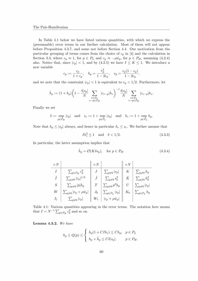
The Pair-Hamiltonian
In Table 4.1 below we have listed various quantities, with which we express the(presumable) error terms in our further calculation. Most of them will not appearbefore Proposition 4.3.7, and some not before Section 4.4. Our motivation from theparticular grouping of terms comes from the choice of cp in [4] and the calculation inSection 3.3, where cp ≈ 1, for p ∈ PL and cp ≈ −ρwp, for p ∈ PH , assuming (4.2.4)also. Notice that, since |cp| < 1, and by (4.2.5) we have I ≤ K ≤ 1. We introduce anew variable
ep :=cp
1 + cp, hp =
e2p
1− 2ep, sp =
ep(1− ep)1− 2ep
,
and we note that the constraint |cp| < 1 is equivalent to ep < 1/2. Furthermore, let
hp := (1 + hp)
(1− 4|sp|
N
∑v∈PL
v−p∈PH
|cv−p|hv)−1 4|sp|
N
∑v∈PL
v−p∈PH
|cv−p|hv.
Finally we set
δ := supp∈PH
|cp| and sc := 1 + supp∈PL
|sp| and hc := 1 + supp∈PL
hp.
Note that hp ≤ |sp| always, and hence in particular hc ≤ sc. We further assume that
Ih2c ≤ 1 and δ < 1/2. (4.3.3)
In particular, the latter assumption implies that
hp = O(Kδsp), for p ∈ PH . (4.3.4)
×N ×N ×N
I∑
p∈PH c2p J
∑p 6=0 |sp| K
∑p 6=0 hp
I∑
p 6=0 |cp|1/2 J∑
p 6=0 s2p K
∑p 6=0 h
2p
S∑
p 6=0 |p|hp T∑
p 6=0 p2hp U
∑p6=0 |ep|
W∑
p 6=0 |ep + ρwp| J0∑
p∈PL |sp| K0∑
p∈PL hp
I1∑
p6=0 |cp| W1 |cp + ρwp|
Table 4.1: Various quantities appearing in the error terms. The notation here meansthat I = N−1
∑p∈PH c
2p and so on.
Lemma 4.3.2. We have
hp ≤ Q(p) ≤
hp(1 + CIhc) ≤ Chp, p ∈ PL
hp + hp ≤ Cδ|sp|, p ∈ PH .
60

The Pair-Hamiltonian
Proof. Notice that Ap(M) ⊆M for each p 6= 0. Then
Q(p) ≥∑
α∈Ap(M)
α(p)|f(α)|2 =∑β∈MApβ(p)|f(Apβ)|2 ≥ c2
p(Q(p) + 1),
where the second inequality comes from the case where p ∈ PL and β ∈Map . It follows
that Q(p) ≥ hp. For the upper bounds, we suppose first that p ∈ PL. Write
Q(p) =∑α∈Ms
p
α(p)|f(α)|2 +∑α∈Ma
p
α(p)|f(α)|2 =: Qs(p) +Qa(p).
Following the argument in the proof of Lemma 4.3.1 (ii) we see that
Qs(p) = hp∑α∈Ms
p
|f(α)|2 ≤ hp.
To estimate Qa(p) we notice that Map is generated from M s
p via soft-pair operations.That is, for each α ∈Ma
p with, say, α∗(p) = α(−p), there exist q ∈ PH with p− q ∈ PHand β ∈M s
p with β(p) ≥ 1, such that α = Ap,qβ. Thus we have the upper bound∑α∈Ma
p
α∗(p)=α(−p)
α(p)|f(α)|2 ≤∑β∈Ms
p
∑q∈PHp−q∈PH
Ap,qβ(p)|f(Ap,qβ)(p)|2 (4.3.5)
=∑β∈Ms
p
∑q∈PHp−q∈PH
(β(p)− 1)β(p)4
N|cq| · |cp−q||f(β)|2
≤ 4I∑β∈Ms
p
(β(p)− 1)β(p)|f(β)|2,
where the equality follows from the relation (4.3.2), and where we have used the Cauchy-Schwarz in the last estimate. Again, by following the strategy used in the proof ofLemma 4.3.1, we obtain∑
β∈Msp
(β(p)− 1)β(p)|f(β)|2 = 2hp∑β∈Ms
p
β(p)|f(β)|2 = 2h2p
∑β∈Ms
p
|f(β)|2 ≤ 2h2p.
It follows that the left-hand side in (4.3.5) is bounded by 8Ih2p. Similarly we bound the
sum where α∗(p) = α(p), but the contribution from this case is 4Ihp(2hp + 1). Usingthe bound hp + 1 ≤ hc we obtain the desired.
Now suppose that p ∈ PH and write
Q(p) =∑
α∈Ap(M)
α(p)|f(α)|2 +∑
α∈M\Ap(M)
α(p)|f(α)|2 =: A+B.
Clearly
A =∑β∈MApβ(p)|f(Apβ)|2 = c2
p(Q(p) + 1), (4.3.6)
61

The Pair-Hamiltonian
and henceQ(p) = hp + (1 + hp)B. (4.3.7)
If α ∈ M\Ap(M) with α(p) ≥ 1, then there exist a v ∈ PL with v − p ∈ PH and aβ ∈M s
v such that Av,pβ = α. Thus B may be bounded as
B ≤∑v∈PL
v−p∈PH
∑β∈Ms
v
Av,pβ(p)|f(Av,pβ)|2
= 4N−1∑v∈PL
v−p∈PH
|cp||cv−p|∑β∈Ms
v
β(v)(β(p) + 1)|f(β)|2
≤ 4N−1|cp|(Q(p) + 1)∑v∈PLv−p∈PL
|cv−p|hv
= 4N−1 |cp|1− c2
p
(B + 1)∑v∈PL
v−p∈PH
|cv−p|hv,
and it follows that B ≤ hp/(1+hp). Together with (4.3.7), this shows the upper boundin case p ∈ PH .
Remark 4.3.3. From Lemma 4.3.1, Lemma 4.3.2 and (4.2.5) it follows that
N ≤ 〈N〉 ≤ N[1 + CK(Ihc + δJ)
].
The estimates in the following lemma can be obtained using the strategy of Lemma4.3.2 and the assumptions in (4.3.3), so we skip the proof. We say that vectorsp1, . . . , pm are ± different if pi 6= ±pj , for each i 6= j.
Lemma 4.3.4. (i) If p1, . . . , pn ∈ PL are ± different, then
Q(p1, . . . , pn) ≤ Chp1Q(p2, . . . , pn).
(ii) If q1, . . . , qm ∈ PH are ± different and p1, . . . , pn /∈ PH , then
Q(p1, . . . , pn, q1, . . . , qm) ≤ Cmδm|cq1 · · · cqm |Q(p1, . . . , pn)
(iii) For p 6= 0,
Q(p,±p) ≤ C ·
hchp, p ∈ PL
δ|sp|, p ∈ PH.
Lemma 4.3.5. We have
〈a+p a
+−p〉 =
sp[1 +O(Ihc)
]if p ∈ PL
sp[1 +O(δ|cp|)
]if p ∈ PH
.
62
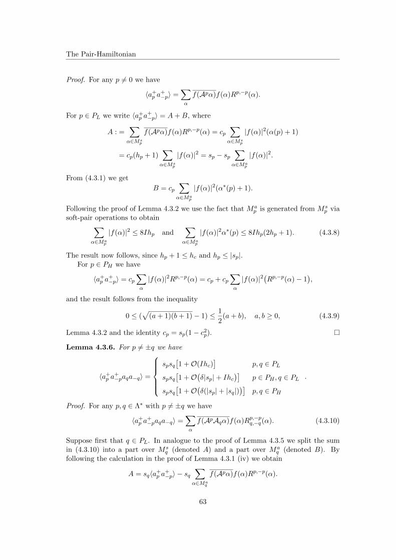
The Pair-Hamiltonian
Proof. For any p 6= 0 we have
〈a+p a
+−p〉 =
∑α
f(Apα)f(α)Rp,−p(α).
For p ∈ PL we write 〈a+p a
+−p〉 = A+B, where
A : =∑α∈Ms
p
f(Apα)f(α)Rp,−p(α) = cp∑α∈Ms
p
|f(α)|2(α(p) + 1)
= cp(hp + 1)∑α∈Ms
p
|f(α)|2 = sp − sp∑α∈Ma
p
|f(α)|2.
From (4.3.1) we get
B = cp∑α∈Ma
p
|f(α)|2(α∗(p) + 1).
Following the proof of Lemma 4.3.2 we use the fact that Map is generated from M s
p viasoft-pair operations to obtain∑
α∈Map
|f(α)|2 ≤ 8Ihp and∑α∈Ma
p
|f(α)|2α∗(p) ≤ 8Ihp(2hp + 1). (4.3.8)
The result now follows, since hp + 1 ≤ hc and hp ≤ |sp|.For p ∈ PH we have
〈a+p a
+−p〉 = cp
∑α
|f(α)|2Rp,−p(α) = cp + cp∑α
|f(α)|2(Rp,−p(α)− 1
),
and the result follows from the inequality
0 ≤ (√
(a+ 1)(b+ 1)− 1) ≤ 1
2(a+ b), a, b ≥ 0, (4.3.9)
Lemma 4.3.2 and the identity cp = sp(1− c2p).
Lemma 4.3.6. For p 6= ±q we have
〈a+p a
+−paqa−q〉 =
spsq
[1 +O(Ihc)
]p, q ∈ PL
spsq[1 +O
(δ|sp|+ Ihc
)]p ∈ PH , q ∈ PL
spsq[1 +O
(δ(|sp|+ |sq|)
)]p, q ∈ PH
.
Proof. For any p, q ∈ Λ∗ with p 6= ±q we have
〈a+p a
+−paqa−q〉 =
∑α
f(ApAqα)f(α)Rp,−pq,−q(α). (4.3.10)
Suppose first that q ∈ PL. In analogue to the proof of Lemma 4.3.5 we split the sumin (4.3.10) into a part over M s
q (denoted A) and a part over Maq (denoted B). By
following the calculation in the proof of Lemma 4.3.1 (iv) we obtain
A = sq〈a+p a
+−p〉 − sq
∑α∈Ma
q
f(Apα)f(α)Rp,−p(α).
63

The Pair-Hamiltonian
Hence
|A− sq〈a+p a
+−p〉| ≤ |sqcp|
∑α∈Ma
q
|f(α)|2(α∗(p) + 1)
≤ 8I|sqcp|∑α∈Ms
q
|f(α)|2α(q)(α∗(p) + 1)
≤ 16Ihq|sqcp|(Q(p) + 1) ≤ CIhq|spsq|. (4.3.11)
For the term B we notice that, if α(q) and α(−q) are both positive, then α ∈ Aq(M).It follows that
|B| ≤ |cpcq|∑β∈Ma
q
|f(β)|2(β∗(p) + 1)(β∗(q) + 1),
and using the fact that Maq is generated from M s
q via soft-pair operations, we can showthat B is also bounded by the the last expression in (4.3.11). The two first claims ofthe lemma then follows from the triangle inequality together with Lemma 4.3.5 andthe relation cp = sp(1− c2
p). For p, q ∈ PH we write
〈a+p a
+−paqa−q〉 = cp
∑α
f(Aqα)f(α)Rp,−pq,−q(α)
= cp∑α
f(Aqα)f(α)Rq,−q(α) + Ω
= cp〈aqa−q〉+ Ω,
where
Ω := cp∑α
f(Aqα)f(α)Rq,−q(α)(Rp,−p(α)− 1
)= cpcq
∑α
|f(α)|2Rq,−q(α)(Rp,−p(α)− 1
)satisfies
|Ω| ≤ 1
2|cpcq|
∑α
|f(α)|2(α∗(q) + 1)(α(p) + α(−p)) ≤ Cδhp|cq|.
Again the result follows from Lemma 4.3.5 and the identity cp = sp(1− c2p).
Recall that for any continuous function F ∈ L1(Rn), decaying faster than |p|−n−εat infinity, for some ε > 0, we have the convergence
limL→∞
1
Ln
∑p∈Λ∗
F (p) =1
(2π)n
∫RnF (p) dp. (4.3.12)
Since we do not take the thermodynamic limit we will get L-dependent errors in ourestimates. In this regard we employ the bound∣∣wp+v − wp∣∣ ≤ C|v|(|p|−2 + |p|−3
),
64

The Pair-Hamiltonian
which holds for each p, v ∈ Rn with |v|/|p| ≤ c < 1. This follows from the Lipschitzcontinuity of g and the fact that |gp| ≤ g0. The relevant sums-to-integral error termsthen turn out to be E3(L) = L−1 lnL and En(L) = L−1, if n ≥ 4.
Proposition 4.3.7. We have
〈HP 〉N≤ EBog +
2ρ
N
∑p6=0
ϕphp +1
N
∑p∈PH
p2hp + ΩP , (4.3.13)
where
EBog :=g0
2ρ+
1
N
∑p 6=0
p2
[e2p + 2ρwpep
1− 2ep+ (ρwp)
2
](4.3.14)
and
ΩP = Cρ
K(K + δJ + Isc) + J2sc(δ + I) + JS
+ ρ−1IT +N−1(J + δJ + scK) +W 2 + UEn(L)
.
Remark 4.3.8. By comparing with Lemma 3.3.6 and ignoring the Ω-terms, we seethat the only new term in the energy of the pair-Hamiltonian is N−1
∑p∈PH p
2hp, cor-responding to some extra kinetic energy (see the proof below).
Proof. By Lemma 4.3.1 and Lemma 4.3.2 we have the following upper bound on thekinetic energy: ∑
p
p2〈a+p ap〉 ≤
∑p
p2hp +∑p∈PH
p2hp + I∑p∈PL
p2hp.
Using the CCR, Lemma 4.3.1 (i), (4.2.5) and the fact that Q(p) ≥ hp ≥ 0 (Lemma4.3.2) we have
〈HP1〉 =V0
2|Λ|
(∑p,q
Q(p, q)−∑p
Q(p)
)
=V0
2|Λ|
(N0(N0 + 1) + 2N0
∑p6=0
Q(p) +∑p,q 6=0
Q(p, q)−∑p 6=0
Q(p)−N0
)
≤ V0
2|Λ|
(N2 + 2N
∑p 6=0
(Q(p)− hp) +∑p,q 6=0
Q(p, q)
).
Similarly,
〈HP2〉 =∑p6=0
ρVpQ(p)−(
1
|Λ|∑p 6=0
VpQ(p)
)∑p6=0
hp +1
2|Λ|∑p,q 6=0
p 6=q
Vp−qQ(p, q)
65
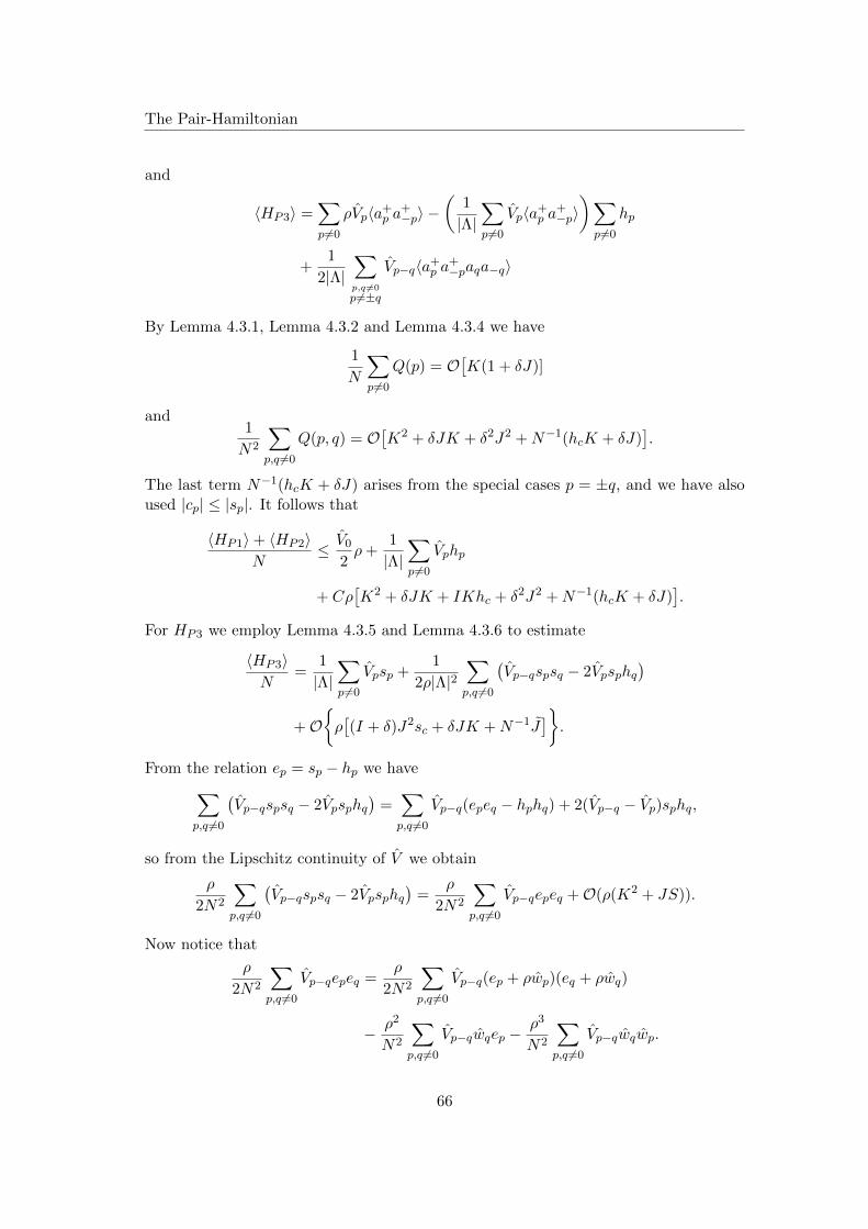
The Pair-Hamiltonian
and
〈HP3〉 =∑p 6=0
ρVp〈a+p a
+−p〉 −
(1
|Λ|∑p 6=0
Vp〈a+p a
+−p〉)∑p 6=0
hp
+1
2|Λ|∑p,q 6=0
p 6=±q
Vp−q〈a+p a
+−paqa−q〉
By Lemma 4.3.1, Lemma 4.3.2 and Lemma 4.3.4 we have
1
N
∑p 6=0
Q(p) = O[K(1 + δJ)]
and1
N2
∑p,q 6=0
Q(p, q) = O[K2 + δJK + δ2J2 +N−1(hcK + δJ)
].
The last term N−1(hcK + δJ) arises from the special cases p = ±q, and we have alsoused |cp| ≤ |sp|. It follows that
〈HP1〉+ 〈HP2〉N
≤ V0
2ρ+
1
|Λ|∑p 6=0
Vphp
+ Cρ[K2 + δJK + IKhc + δ2J2 +N−1(hcK + δJ)
].
For HP3 we employ Lemma 4.3.5 and Lemma 4.3.6 to estimate
〈HP3〉N
=1
|Λ|∑p 6=0
Vpsp +1
2ρ|Λ|2∑p,q 6=0
(Vp−qspsq − 2Vpsphq
)+O
ρ[(I + δ)J2sc + δJK +N−1J
].
From the relation ep = sp − hp we have∑p,q 6=0
(Vp−qspsq − 2Vpsphq
)=∑p,q 6=0
Vp−q(epeq − hphq) + 2(Vp−q − Vp)sphq,
so from the Lipschitz continuity of V we obtain
ρ
2N2
∑p,q 6=0
(Vp−qspsq − 2Vpsphq
)=
ρ
2N2
∑p,q 6=0
Vp−qepeq +O(ρ(K2 + JS)).
Now notice that
ρ
2N2
∑p,q 6=0
Vp−qepeq =ρ
2N2
∑p,q 6=0
Vp−q(ep + ρwp)(eq + ρwq)
− ρ2
N2
∑p,q 6=0
Vp−qwqep −ρ3
N2
∑p,q 6=0
Vp−qwqwp.
66

The Anti-Symmetric Interaction Terms
Moreover, since (2π)nϕ = V ∗ w and V = g + ϕ, we get
V
2ρ =
g
2ρ+
ρ
2(2π)n
∫Vpwp dp =
g
2ρ+
ρ
2(2π)n
∫gpwp dp+
ρ
2(2π)n
∫ϕpwp dp.
Finally, by adding up terms and by noting that
1
|Λ|∑p 6=0
Vp−qwq =1
(2π)2
∫Vp−qwq dq +O(En(L)),
the result follows.
4.4 The Anti-Symmetric Interaction Terms
In this section we estimate the energy of the remaining part of the Hamiltonian,
HA := H −HP ,
i.e. the interaction terms from (4.0.2) where p 6= r, s,−q. From HA we further single outterms with (exactly) one zero-momentum operator. Thus we write HA = HA1 +HA2,where
〈HA1〉 =2
|Λ|∑p+q=rp6=r,−q,0
Vq · Re 〈a+p a
+q ara0〉. (4.4.1)
4.4.1 Interaction with Three Non-zero Momenta
We start by noting that in (4.4.1) only terms with p, q, r ∈ PL ∪ PH give nonzerocontribution, due to the fact that α(−p) = α(p), for each α ∈ M and p /∈ PL ∪ PH .Moreover, by construction, for any α ∈M ,
∑k∈PH α(k) is an even number, and hence
we can assume that either none, or exactly two of the momenta p, q, r are containedin PH . Thus, the only relevant expectations are the ones considered in the followinglemma.
Lemma 4.4.1. Suppose that p, q, r are ± different with p+ q = r.
(i) For p, q ∈ PH and r ∈ PL,
〈a+p a
+q ara0〉 = 2
√N0/N
√cp√cqhr
[1 +O
(Ihr + δ2|cr|−1
)].
(ii) For q ∈ PL and p, r ∈ PH ,
〈a+p a
+q ara0〉 = O
(δ|cpcr|1/2|sq|
).
(iii) For p, q, r ∈ PL,〈a+p a
+q ara0〉 = O
((I +N−1)|spsqsr|
).
67

The Anti-Symmetric Interaction Terms
Proof. By Lemma 4.3.1 we have
〈a+p a
+q ara0〉 =
√N0
∑α
f(Ar,pα)f(α)Rp,qr (α). (4.4.2)
Suppose first that p, q ∈ PH and r ∈ PL. We split the sum in (4.4.2) into two parts Aand B depending on whether α ∈M s
r respectively α ∈Mar .
A :=√N0
∑α∈Ms
r
f(Ar,pα)f(α)Rp,qr (α)
= 2√N0/N
√cp√cq∑α∈Ms
r
|f(α)|2α(r)Rp,q(α)
= 2√N0/N
√cp√cqhr
∑α∈Ms
r
|f(α)|2Rp,q(α)
= 2√N0/N
√cp√cqhr
[1 +O
(Ihr + δ(|sp|+ |sq|)
)],
where we in the estimate have used (4.3.9), Lemma 4.3.2 and the first bound in (4.3.8).For the sum over Ma
r we note that
α ∈Mar : Ar,pα ∈M = Ar,p(M s
r ) ∩M, (4.4.3)
where Ar,p := (Ar,p)−1 with
f(Ar,pα) =cr√cp√cq
√4(α(r) + 1)
Nf(α), for α ∈M s
r .
Thus
B =√N0
∑α∈Ms
r
f(α)f(Ar,pα)Rrp,q(α)
= 2√N0/Ncrc
−1/2p c−1/2
q
∑α∈Ms
r
|f(α)|2(α(r) + 1)Rp,q(α)
= 2√N0/Nsrc
−1/2p c−1/2
q
∑α∈Ms
r
|f(α)|2Rp,q(α),
where we have also used sr = cr(hr + 1) in the last equality. From Lemma 4.3.2 and1/(1− c2
p) ≤ C, for p ∈ PH , we see that
B = O[√
N0/N√cp√cqhrδ
2c−1r
].
Upon adding A and B and using |sp|+ |sq| ≤ Cδ and 1 < |cr|−1, we arrive at (i).The case where q ∈ PL and p, r ∈ PH is similar: The sum in (4.4.2) is now splitted
in parts over M sq and Ma
q . For α ∈M sq and Ar,pα ∈M we then have relation
f(Ar,pα) =2cq√cp√
cr
√α(q) + 1
Nf(α).
68
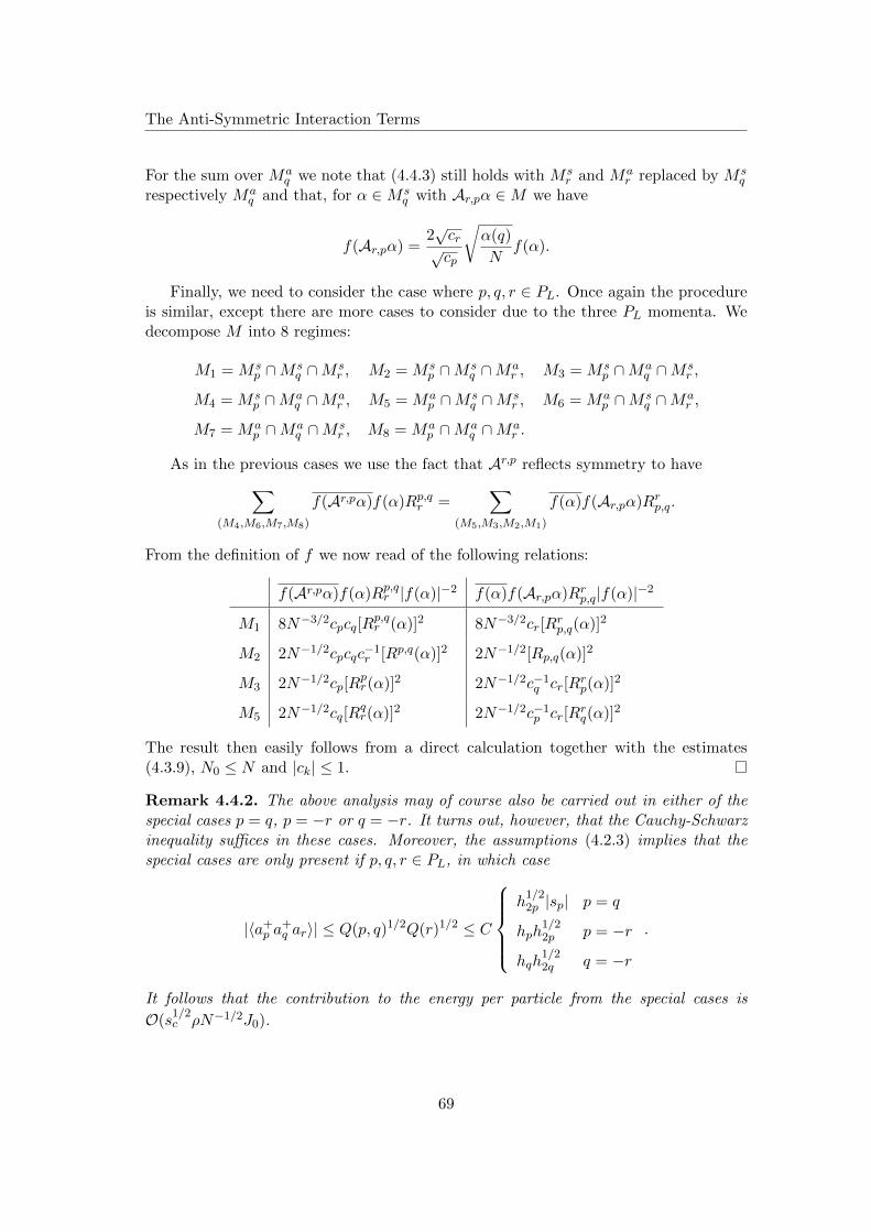
The Anti-Symmetric Interaction Terms
For the sum over Maq we note that (4.4.3) still holds with M s
r and Mar replaced by M s
q
respectively Maq and that, for α ∈M s
q with Ar,pα ∈M we have
f(Ar,pα) =2√cr√cp
√α(q)
Nf(α).
Finally, we need to consider the case where p, q, r ∈ PL. Once again the procedureis similar, except there are more cases to consider due to the three PL momenta. Wedecompose M into 8 regimes:
M1 = M sp ∩M s
q ∩M sr , M2 = M s
p ∩M sq ∩Ma
r , M3 = M sp ∩Ma
q ∩M sr ,
M4 = M sp ∩Ma
q ∩Mar , M5 = Ma
p ∩M sq ∩M s
r , M6 = Map ∩M s
q ∩Mar ,
M7 = Map ∩Ma
q ∩M sr , M8 = Ma
p ∩Maq ∩Ma
r .
As in the previous cases we use the fact that Ar,p reflects symmetry to have∑(M4,M6,M7,M8)
f(Ar,pα)f(α)Rp,qr =∑
(M5,M3,M2,M1)
f(α)f(Ar,pα)Rrp,q.
From the definition of f we now read of the following relations:
f(Ar,pα)f(α)Rp,qr |f(α)|−2 f(α)f(Ar,pα)Rrp,q|f(α)|−2
M1 8N−3/2cpcq[Rp,qr (α)]2 8N−3/2cr[R
rp,q(α)]2
M2 2N−1/2cpcqc−1r [Rp,q(α)]2 2N−1/2[Rp,q(α)]2
M3 2N−1/2cp[Rpr(α)]2 2N−1/2c−1
q cr[Rrp(α)]2
M5 2N−1/2cq[Rqr(α)]2 2N−1/2c−1
p cr[Rrq(α)]2
The result then easily follows from a direct calculation together with the estimates(4.3.9), N0 ≤ N and |ck| ≤ 1.
Remark 4.4.2. The above analysis may of course also be carried out in either of thespecial cases p = q, p = −r or q = −r. It turns out, however, that the Cauchy-Schwarzinequality suffices in these cases. Moreover, the assumptions (4.2.3) implies that thespecial cases are only present if p, q, r ∈ PL, in which case
|〈a+p a
+q ar〉| ≤ Q(p, q)1/2Q(r)1/2 ≤ C
h
1/22p |sp| p = q
hph1/22p p = −r
hqh1/22q q = −r
.
It follows that the contribution to the energy per particle from the special cases is
O(s1/2c ρN−1/2J0).
69

The Anti-Symmetric Interaction Terms
Proposition 4.4.3. We have
〈HA1〉N
= −4K0ϕ0ρ+O(ΩA1
), (4.4.4)
where
ΩA1 := ρK2 + ρJ0
[√δI(Isc + δI) + J0sc(I +N−1) + scN
−1/2]
+
ρK[εH +R−2
H +RL + L−1 ln(L) + W]
+ ρS| ln(εH)|, n = 3
ρK[εn−2H +R−2
H + εHRL + L−1 + W]
+ ρS, n ≥ 4.
Proof. Notice that√N0/N = 1 +O(K). Then, From Lemma 4.4.1 and Remark 4.4.2
above we arrive at the following estimate on the energy per particle of HA1:
〈HA1〉N
=[1 +O(K)
] 4ρ
N2
∑p,q∈PHp+q∈PL
Vqhp+qRe(√cp√cq)
+O(ΩA1) (4.4.5)
whereΩA1 := ρJ0
[√δI(Isc + δI) + J0sc(I +N−1) + scN
−1/2].
Suppose that p, q ∈ PH with r := p+ q ∈ PL. We claim that
Re (√cp√cq) = −ρwq +O
[|cp + ρwp|+ |cq + ρwq|+ ρ|r|(|q|−2 + |q|−3)
]. (4.4.6)
To see this, first notice that∣∣Re(√cp√cq)
+ ρwq∣∣ ≤ ∣∣√cp√cq − cq∣∣+
∣∣cq + ρwq∣∣.
Now, if cp and cq have different sign, then |cp|+ |cq| = |cp − cq| and hence∣∣√cp√cq − cq∣∣ ≤√|cp| |cq|+ |cq| ≤ 2|cp − cq|.
In case cp and cq have the same sign, we have∣∣√cp√cq − cq∣∣ =√|cq| ·
∣∣√|cp| −√|cq|∣∣ ≤ ∣∣cp − cq∣∣,so in either case ∣∣√cp√cq − cq∣∣ ≤ 2|cp − cq|. (4.4.7)
Recall the estimate ∣∣wp+v − wp∣∣ ≤ C|v|(|p|−2 + |p|−3), (4.4.8)
for each p, v ∈ Rn with |v|/|p| ≤ c < 1. Then (4.4.6) follows from the triangle inequalityand (4.4.8). As a consequence the factor Re
(√cp√cq)
in (4.4.5) can be replaced by−ρwq by at cost of an error O[ρKW1 +ρ2S| ln εH |] in three dimensions and O[ρKW1 +ρ2S] in higher dimensions. Furthermore, the summation over p, q ∈ PH with p+q ∈ PLcan be replaced by the summation over PH × PL at the cost of an error O(ρKRL) inthree dimensions and O(ρKεHRL) in higher dimensions. Finally, we note that sinceV ∗ w = (2π)nϕ, we have
1
|Λ|∑q∈PH
Vqwq = ϕ0 +O(εn−2H +R−2
H + En(L)),
and the result follows.
70

The Anti-Symmetric Interaction Terms
4.4.2 Interactions with Four Non-zero Momenta
In this section we estimate the energy of
HA2 =1
2|Λ|∑
(p,q,r,s)∈R
Vp−ra+p a
+q aras, (4.4.9)
whereR :=
(p, q, r, s) ∈ (Λ∗\0)4 : p+ q = r + s, p 6= −q, r, s
.
As for the interactions with three non-zero momenta, we begin by noting that, sincea+p a
+q aras breaks symmetry in p, q, r, s, only terms with p, q, r, s ∈ PL∪PH give nonzero
contribution to the expectation of (4.4.9) in our trial state. Moreover, since each α ∈Mrepresents a state with an even number of particles in PH , we may assume that PHcontains exactly either zero, two or four of the momenta’s p, q, r, s. This leads to adecomposition
HA2 = H0A2 +H2
A2 +H4A2.
Throughout this section we let
Tα = Tp,q,r,sα := α+ δp + δq − δr − δs.
Using the strategy from the proof of Lemma 4.4.1 in the case p, q, r ∈ PL (only here wehave to partition M into 16 different regimes), we obtain
〈a+p a
+q aras〉 = O
[|spsqsrss|
(I2 + IN−1 +N−2
)],
whenever p, q, r, s ∈ PL are ± different. The special cases are easily estimated by theCauchy-Schwarz inequality. This leads to the following estimate on H0
A2.
Lemma 4.4.4. We have
〈H0A2〉N
= O[ρscJ
30 (NI2 + I +N−1)
].
Lemma 4.4.5. We have
〈H2A2〉N
= O[ρδ1/2I
[K2 + δIJ0(J0 + δK)N + δ(K + J0)
]]. (4.4.10)
Proof. Suppose first that p, q ∈ PL and r, s ∈ PH . The only special case possible isp = q, in which case the Cauchy-Schwarz inequality yields
|〈a+p a
+p aras〉| ≤ Q(p, p)1/2Q(r, s)1/2 ≤ Cδ|sp|
√|crcs|.
Suppose now that p 6= q (and hence p, q, r, s are ± different). Then
〈a+p a
+q aras〉 =
∑α
f(Tα)f(α)Rp,qr,s (α). (4.4.11)
Decompose M into 4 regimes,
M1 = M sp ∩M s
q , M2 = M sp ∩Ma
q , M3 = Map ∩M s
q , M4 = Map ∩Ma
q .
71

The Anti-Symmetric Interaction Terms
For α ∈M1 we have the relation
f(Tα) =4
N
cpcq√cr√csRp,q(α)f(α),
and hence the contribution to (4.4.11) from this regime is∣∣∣∣ ∑α∈M1
· · ·∣∣∣∣ =
4
N
|cpcq|√|crcs|
∑α∈M1
(α(p) + 1)(α(q) + 1)Rr,s(α)|f(α)|2
≤ 4
N
|spsq|√|crcs|
Q(r, s) ≤ CN−1δ2|spsq|√|crcs|.
Next, for α ∈M2,
f(Tα) =cp√cr√cs
√α(p) + 1
α(q) + 1f(α),
and hence ∣∣∣∣ ∑α∈M2
· · ·∣∣∣∣ =
|cp|√|crcs|
∑α∈M2
|f(α)|2(α(p) + 1)Rr,s(α)
≤ |sp|√|crcs|
∑α∈Ma
q
|f(α)|2α(r)α(s)
≤ CIδ2|sp|hq√|crcs|.
In the last inequality, the factor Ihq comes from the fact that Maq is generated from
M sq via soft-pair creations. The contribution from M3 equals the contribution from M2
with p and q interchanged. For the last case we use∑α∈M4
· · · =∑β∈M1
f(β)f(T−1β)√β(p)β(q)(β(r) + 1)(β(s) + 1)
to obtain ∣∣∣∣ ∑α∈M4
· · ·∣∣∣∣ ≤ CN−1hphq
√|cr|√|cs|.
In total we have
|〈a+p a
+q aras〉| ≤ C
√|crcs|
[N−1hphq + Iδ2(hq|sp|+ hp|sq|) + δ2N−1|spsq|
].
The case p, r ∈ PL and q, s ∈ PH is similar: In the special case p = −r we have
|〈a+p a
+q a−pas〉| ≤ Cδhp
√|cqcs|,
and otherwise
|〈a+p a
+q aras〉| ≤ C
√|cqcs|
[δN−1
(|sp|hr + hp|sr|
)+ δI|spsr|
].
By carrying out the appropriate integrations, we arrive at the desired.
72

The Anti-Symmetric Interaction Terms
Lemma 4.4.6. Suppose that δ2ρ−1|Λ|R3n/2L R
n/2H ≤ ρε, for some ε > 0. Then
〈H4A2〉N
=2ρK0
(2π)n
∫ϕpwp dp+O(Ω4
A2), (4.4.12)
where
Ω4A2 := ρδI2
[δ2 +K(Ihc + δ2)
]+R3n
H δ4ρ−2
[1 + ρ−1h2
cRnL
]+ ρKW1
[1 + I1 + δ1/2I
]+ ρK
[εn−2H +R−2
H + En(L)]
+ ρS[I1 + δ1/2I
]×
[RH + ln(RH/εH)
], n = 3[
Rn−2H +Rn−3
H
], n ≥ 4
.
Proof. Notice that, for p, q, r, s ∈ PH ,
f(Tα) =
√cp√cq√
cr√csf(α),
whenever Tα ∈ M . There are essentially only two special cases to consider, namelyp = q and p = −r, and it is easy to see that
|〈a+p a
+q aras〉| ≤ Cδ2|cp|
√|crcs| if p = q√|cqcs| if p = −r
.
It follows that the contribution to the energy per particle from the special cases isO(δ3ρI2). Now fix (p, q, r, s) ∈ R such that p, q, r, s ∈ PH are ± different. Then
〈a+p a
+q aras〉 =
∑α
f(Tα)f(α)Rp,qr,s (α) = A+B,
whereA :=
∑α∈M ′
f(Tα)f(α)Rp,qr,s (α), B :=∑
α∈M\M ′f(Tα)f(α)Rp,qr,s (α)
and M ′ := Ar+s,r(M sr+s), if r + s ∈ PL, and M ′ := ∅ otherwise. We will see that
the main contribution comes from the term A. Suppose that r + s ∈ PL. SinceT = Ap+q,pAr+s,r, we have
A =∑
β∈Msr+s
f(Ap+q,pβ)f(Ar+s,rβ)Rr,s(β)Rp,q(β)
= ±4N−1√cp√cq√cr√cshp+q
∑β∈Ms
p+q
|f(β)|2Rr,s(β)Rp,q(β),
where the negative sign applies in case cp and cq have different sign. From (4.3.9) itfollows that
0 ≤√
(a+ 1)(b+ 1)(c+ 1)(d+ 1)− 1 ≤ 1
2
(ab+ a+ b+ cd+ c+ d
),
73

The Anti-Symmetric Interaction Terms
for nonnegative a, b, c, d. Using this fact and (4.3.8) we obtain
A = ±4N−1√cp√cq√cr√cshp+q
+O(N−1hp+q|cpcqcrcs|1/2
[δ(|cr|+ |cs|+ |cp|+ |cq|) + Ihp+q
]). (4.4.13)
With two integrations over PH and one integration over PL, the contribution to theenergy per particle from the error in (4.4.13) is of order ρδI2K(Ihc + δ2). Using thetriangle inequality, (4.4.7) and (4.4.8), we obtain
±√cp√cq√cr√cs = ρ2wpwr +O
|cr| |cp + ρwp|+ ρ|wp| |cr + ρwr| (4.4.14)
+√|crcs|
(|cp + ρwp|+ ρ|p+ q|(|p|−2 + |p|−3) + |cq + ρwq|
)+ |cp|
(|cr + ρwr|+ ρ|r + s|(|r|−2 + |r|−3) + |cs + ρws|
).
The contribution to the energy per particle from the error in (4.4.14) is of order
ρKW1
(1 + I1 + δ1/2I
)+ ρS
(I1 + δ1/2I
)×
[RH + ln(RH/εH)
], n = 3[
Rn−2H +Rn−3
H
], n ≥ 4
.
Furthermore, we have
2
N3
∑p,q,r,s∈PHp+q=r+s
Vp−rwrwphp+q =2ρK0
(2π)3
∫ϕpwp dp+O
[ρK(εn−2H +R−2
H + En(L))].
In order to estimate the term B we employ the fact that∑α(r)≥m
|f(α)|2Rp,qr,s (α) = O[δ|cs|(δ|cr|)m
], m ≥ 0, (4.4.15)
and the analogues bounds for sums over α(s) ≥ m, α(p) ≥ m and α(q) ≥ m. Theseestimates are easy, but tedious, to obtain using the strategy of Lemma 4.3.2 and |cp| ≤ δ,for p ∈ PH . As a consequence we may restrict attention to α’s which are boundeduniformly in p, q, r, s, and hence it suffices to show that
B :=∑
α∈M\M ′|f(Tα)f(α)|
is negligible. Given m ∈ N0, a nonempty subset v1, . . . , vt ⊂ PL of ± differentelements and a γ ∈ M with γ(−vi) = γ(vi) ≥ 1, we let M(m, v1, . . . , vt, γ) denotethe set of all α ∈M\M ′ such that α and Tα have the form
α =
t∏i=1
Avi,kim∏j=1
Aqjγ, Tα =
t∏i=1
Avi,k′im∏j=1
Aq′jγ. (4.4.16)
74

The Anti-Symmetric Interaction Terms
Here qj , ki, (vi − ki) are in PH and similarly for the ’primes’. We also require that
ki 6= k′i and qj 6= q′j . (4.4.17)
In case m = 0 the products over j in (4.4.16) should be interpreted as a factor one.Notice also that if m = 0, then t ≥ 2, since otherwise α ∈M ′. From the definition of fand the fact that |ck| ≤ δ whenever k ∈ PH , we see that, for α ∈M(m, v1, . . . , vt, γ),
|f(Tα)f(α)| ≤ δ2m[4δ2N−1
]t|f(γ)|2t∏i=1
γ(vi).
Since α and Tα agree outside PH and represent states with equal number of particlesin PH , it follows that
α ∈M\M ′ : Tα ∈M ⊆⋃
m,v1,...,vt,γ
M(m, v1, . . . , vt, γ),
and hence we have an upper bound
B ≤∑
m,v1,...,vt,γ
δ2m[4δ2N−1
]t|f(γ)|2t∏i=1
γ(vi) · |M(m, v1, . . . , vt, γ)|,
where | · | denotes the cardinality. We claim that
|M(m, v1, . . . , vt, γ)| ≤ |PH |−1t![Ct|PH |
]t/2 · [C|PH |]m/2, (4.4.18)
if there exists an i ∈ 1, . . . , t such that
vi ∈ span0,±1 v1, . . . , vi−1, vi+1, . . . , vt, p, q, r, s, (4.4.19)
and |M(m, v1, . . . , vt, γ)| = 0 otherwise. Here span0,±1 denotes the set of all linearcombinations with coefficients in 0, 1,−1. To verify (4.4.18) we suppose that α ∈M(m, v1, . . . , vt, γ) so that α and Tα has the form (4.4.16). Since in particularα /∈M ′ we must have
ki, vi − ki 6= r, s and k′i, vi − k′i 6= p, q. (4.4.20)
Since Tα(k) = α(k), for each k /∈ p, q, r, s, the PH -momenta in the representation forα respectively Tα in (4.4.16) are almost the same. We denote the common momenta byp1, . . . , p2(m+t)−2. Counting with multiplicity, the PH -momenta appearing in (4.4.16)for α respectively Tα can then be listed as
α : r, s, p1, . . . , p2(m+t)−2
Tα : p, q, p1, . . . , p2(m+t)−2
Thus each common momenta appear in one α-pair and one Tα-pair. By (4.4.20), themomenta p, q, r, s form pair with one common momenta each. A ’graph’ is associated
75
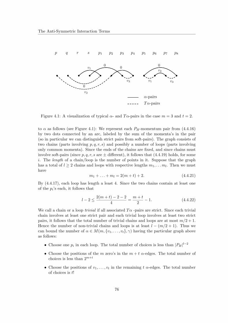
The Anti-Symmetric Interaction Terms
s s s s s s s s s s s s
p q r s p1 p2 p3 p4 p5 p6 p7 p8
.......................
.........................................
................... .................. .................. ................... .................... .......................................
....
v1
...........................
.................................................
............................................. ..................... .................... ..................... ...................... .......................
............................................
.....
..........................
0
.......................
.........................................
................... .................. .................. ................... .................... .......................................
....
0
...........................
.................................................
............................................. ..................... .................... ..................... ...................... .......................
............................................
.....
..........................
0
. ............................... .............. ............ .............. ............... ................v2
............ ............ ........... ............ ........... ........... ........... .......... .......... .......... .......... .......... .......... .......... .......... .......... .......... .......... .......... ..................... ........... ........... ............
.......................
............
v2
............ ......................... ........... ............ ....................... .......... .................... .......... ........... ....................... ........... .............
........... ..................
0
............ ........... .......... .......... ....................
v3
............ ........... .......... .......... ....................
v1
............ ........... .......... .......... ....................
v3
α-pairs
.......... .......... .......... .......... .......... Tα-pairs
Figure 4.1: A visualization of typical α- and Tα-pairs in the case m = 3 and t = 2.
to α as follows (see Figure 4.1): We represent each PH -momentum pair from (4.4.16)by two dots connected by an arc, labeled by the sum of the momenta’s in the pair(so in particular we can distinguish strict pairs from soft-pairs). The graph consists oftwo chains (parts involving p, q, r, s) and possibly a number of loops (parts involvingonly common momenta). Since the ends of the chains are fixed, and since chains mustinvolve soft-pairs (since p, q, r, s are ± different), it follows that (4.4.19) holds, for somei. The length of a chain/loop is the number of points in it. Suppose that the graphhas a total of l ≥ 2 chains and loops with respective lengths m1, . . .ml. Then we musthave
m1 + . . .+ml = 2(m+ t) + 2. (4.4.21)
By (4.4.17), each loop has length a least 4. Since the two chains contain at least oneof the pi’s each, it follows that
l − 2 ≤ 2(m+ t)− 2− 2
4=m+ t
2− 1. (4.4.22)
We call a chain or a loop trivial if all associated Tα -pairs are strict. Since each trivialchain involves at least one strict pair and each trivial loop involves at least two strictpairs, it follows that the total number of trivial chains and loops are at most m/2 + 1.Hence the number of non-trivial chains and loops is at least l − (m/2 + 1). Thus wecan bound the number of α ∈M(m, v1, . . . , vt, γ) having the particular graph aboveas follows:
• Choose one pi in each loop. The total number of choices is less than |PH |l−2
• Choose the positions of the m zero’s in the m + t α-edges. The total number ofchoices is less than 2m+t
• Choose the positions of v1, . . . , vt in the remaining t α-edges. The total numberof choices is t!
76

The Anti-Symmetric Interaction Terms
• Choose the positions of the m zero’s in the m+ t Tα-edges. The total number ofchoices is less than 2m+t
• Choose the positions of the vi’s in Tα-edges. The total number of choices is lessthan tt−(l−m/2−1)
Taking the product of the above yields
4m+tt!|PH |−2tt+m/2+1(|PH |/t
)l ≤ |PH |−1t![16t|PH |
]t/2[16|PH |
]m/2, (4.4.23)
where the inequality follows from (4.4.22), assuming that |PH |/t ≥ 1. Since the right-hand side in (4.4.23) is independent of m1, . . . ,ml and l, we only need to show thatthe number of different graphs is bounded by Cm+t. But this follows by considering(for fixed l) the number of nonnegative integer solutions to (4.4.23), summing froml = 2, . . . , (m+ t)/2 + 1 and then using the binomial theorem.
Employing the bound (4.4.18) we now can finish the proof as follows: First performthe summation over γ,
∑γ∈∩iMs
vi
|f(γ)|2t∏i=1
γ(vi) ≤ htc∑
γ∈∩iMsvi
|f(γ)|2 ≤ htc. (4.4.24)
Next we note that, for fixed t, the number of subsets v1, . . . , vt ⊂ PL with the propertythat (4.4.19) holds, for some i, is bounded by
t3t+3 |PL|t−1
(t− 1)!.
Thus we have
B ≤ C
|PL| · |PH |∑t≥1
∑m≥0
m+t≥2
[Cδ2|PH |1/2
]m[Cδ2hcN
−1|PL|(t|PH |)1/2]t
≤ Cδ4N−1 +C
|PL| · |PH |∑t≥2
[Cδ2hcN
−1|PL|(t|PH |)1/2]t.
Let t0 ≥ 2 and notice that∑2≤t≤t0
[Cδ2hcN
−1|PL|(t|PH |)1/2]t ≤ Ct0δ4h2
c |PL|2|PH |N−2,
provided δ2hcN−1|PL|(t0|PH |)1/2 is sufficiently small (which is true if µ below is small).
For the remaining part of the sum, we use t ≤ |PL| to obtain∑t>t0
[Cδ2hcN
−1|PL|(t|PH |)1/2]t ≤ Cµt0 ,
providedµ := Cδ2hcN
−1|PL|3/2|PH |1/2
77

Minimization and Estimates
is sufficiently small. In total we get
B|PH |3
N |Λ|≤(|PH ||Λ|
)3[δ4ρ−2 + t0δ
4ρ−3h2c
|PL||Λ|
+|Λ|
|PH ||PL|ρ−1µt0
]From the bounds |PL| ∼ |Λ|RnL and |PH | ∼ |Λ|RnH we see that∣∣∣∣ 1
N |Λ|∑
p,q,r,s∈PHp+q=r+s
B
∣∣∣∣ ≤ CR3nH δ
4ρ−2(1 + ρ−1h2
cRnL
),
provided µ ≤ ρε and t0 sufficiently large. Also notice that
µ ≤ Cδ2ρ−1|Λ|R3n/2L R
n/2H .
By adding up the error terms we are finally done.
4.5 Minimization and Estimates
Considering (4.3.13) we start by noting that
2ρ
N
∑p 6=0
ϕphp = 2ρK0ϕ0 +O[ρ(K −K0) + ρS
]. (4.5.1)
For the excess kinetic energy we have
1
N
∑p∈PH
p2hp =[1 +O(δ2)
] 4
N2
∑p∈PH
p2|sp|∑v∈PL
v−p∈PH
|cv−p|hv
=[1 +O(δ2)
]( 2K0ρ
(2π)n
∫gpwp dp+O(ΩKin)
), (4.5.2)
where
ΩKin :=1
N2
∑p∈PH
∑v∈PL
v−p∈PH
p2|sp|∣∣cv−p − cp∣∣hv +
K
N
∑εH≤|p|≤εH+RL
p2hp
+K
N
∑RH−RL≤|p|≤RH
p2hp +Kρ
|Λ|∑p/∈PH
gpwp
+K
N
∑p∈PH
p2[hp − (ρwp)
2]
+KρEn(L).
Upon adding the (presumable) main terms from (4.5.1), (4.5.2), (4.4.12) and (4.4.4),and by using (2π)nϕ = V ∗ w, we see that they exactly cancel:
2ρK0ϕ0 +2K0ρ
(2π)n
∫gpwp dp+
2ρK0
(2π)3
∫ϕpwp dp− 4K0ϕ0ρ = 0.
78

Minimization and Estimates
We choose the function ep pointwise to minimize the expression
mp :=e2p + 2ρwpep
1− 2ep.
from (4.3.14). This yields
−e2p + ep + ρwp = 0, ep =
1
2
(1−
√1 + 4ρwp
)(4.5.3)
and
mp =1
2
(√1 + 4ρwp − 1− 2ρwp
),
provided 1 + 4ρwp ≥ 0. Note however that, since g is continuous, g0 > 0 and gp → 0 as|p| → ∞, it follows that wp is bounded from below, and hence
lim infρ→0
[infp 6=0
(1 + 4ρwp)]≥ 1.
Notice that (4.5.3) yields
cp =1−
√1 + 4ρwp
1 +√
1 + 4ρwp, sp =
−ρwp√1 + 4ρwp
, hp =1
2
(1 + 2ρwp√1 + 4ρwp
− 1
). (4.5.4)
Also notice thatcp = −ρwp +O((ρwp)
2) as ρp−2 → 0.
Finally, with the choice in (4.5.3) we have
EBog =g0
2ρ+
1
2ρ|Λ|∑p 6=0
p2Φ(ρwp), (4.5.5)
whereΦ(t) :=
√1 + 4t+ 2t2 − 2t− 1. (4.5.6)
Notice that ρwp ≤ g0ρε−2L /2, for any p ∈ PL. Suppose that RL 1 such that also
ρwp > 0 whenever p ∈ PL. Then
sc = supp∈PL
|sp| = O(ρ1/2ε−1L )
In Table 4.2 we have listed elementary estimates on the quantities from Table 4.1, giventhe particular choice in (4.5.3) (see also [4] and Section 3.3.3).
4.5.1 Dimension n = 3
A straightforward calculation, using the fact that Φ is increasing and gp ≤ g0, yields
EBog ≤ 4πaρ
(1 +
128
15√π
(a3ρ)1/2
)+O
[ρ3/2(lnL)/L
],
79

Minimization and Estimates
I J K S T U W J0
n = 3 ρε−1H 1 ρ1/2 ρ ln ρ ρ 1 ρ1/2 RL
n = 4 ρε−1H 1 ρ ln ρ ρ ρ 1 ρ ln ρ R2
L
I J K W1 I1 sc hc δ
n = 3 ρ−1/2 ρ1/2 ρ1/2 ρ1/2 1 ρ1/2ε−1L ρ1/2ε−1
L ρε−2H
n = 4 ρ−1/2 ρ ln ρ ρ ln ρ ρ ln ρ 1 ρ1/2ε−1L ρ1/2ε−1
L ρε−2H
Table 4.2: Estimates on the quantities from Table 4.1. The information here is thatI = O(ρε−1
H ), for n = 3, and so on.
where the error ρ3/2(lnL)/L comes from replacing the sum with an integral. We nowchoose parameters. From (4.5.1) we need K ≈ K0, and since the main contributionto the sum defining K comes from |p| ∼ ρ1/2, we choose εL, RL ∼ ρ1/2. From ΩA1
in Proposition 4.4.3 and ΩA2 in Lemma 4.4.6, it is clear that we need εH 1 andR−1H 1. However, from the estimates on I and δ in Table 4.2 it is also clear that εH
cannot be too small, which in turns implies that RH cannot be too large. In particular,if we take RH = ε−1
H , then the second term in ΩA2 together with δ = O(ρε−2H ) shows
that εH ≥ ρ1/34. For simplicity we choose
εL = ρ1/2+η, RL = ρ1/2−η, εH = ρη and RH = ρ−η
for some 0 < η ≤ 1/34. Moreover we take L = ρ−(1+η). With these choices we obtain
ΩP = O(ρ2−3η) and ΩA1 = O(ρ3/2+η).
Furthermore, the contributions from Lemma 4.4.4 and Lemma 4.4.5 are O(ρ5/2−9η)respectively O(ρ2−9η). The condition in Lemma 4.4.6 is satisfied if η < 1/52 and thecontribution is then ΩA2 = O(ρ3/2+η). Finally, one can check that the errors from(4.5.1) and (4.5.2) are also of order ρ3/2+η. This concludes the proof of Theorem 4.1.3.
4.5.2 Dimension n = 4
In 4 dimensions we have (see Section 3.3.3)
EBog ≤ 4π2a2ρ
(1 + 2π2a4ρ| ln(a4ρ)|
)+O
[ρ2(1 + | ln ρ|L−1)
].
Proceeding similarly to the 3-dimensional case, we seek parameters such that K ≈ K0.However, in 4 dimensions, the dominant part of
∑p 6=0 hp comes from the regime ρ1/2 ≤
|p| ≤ 1, and hence we are forced to take RL ∼ 1. Furthermore, we have the estimate
ΩP = O(ρ2ε−3H + ρL−1),
80

Proof of Lemma 4.1.1
similar to the 3-dimensional case, so we must also have εH ∼ 1 and L ∼ ρ−1. Onthe other hand, since J0 = R2
L, we see that the estimates in Section 4.4.6 all requireRL ∼ ρα, for some 1/4 ≤ α ≤ 1/2. A further complication arises when we attemptto divide Λ into smaller boxes (since we cannot take the thermodynamic limit). WithL = ρ−γ , we could repeat the steps from Section 4.1 to show that
e0(ρ) ≤ 4π2a2ρ
(1 + 2π2a4ρ| ln(a4ρ)|
)+ Ω + Cρ1/2+γ ,
where Ω denotes the sum of all ’error terms’. Thus, in 4 dimensions we need γ ≈ 3/2,in contrast to γ ≈ 1 in 3 dimensions. This makes an appropriate choice of parameterseven harder, if not impossible.
4.A Proof of Lemma 4.1.1
Define the function q : R→ [0, 1] by
q(t) =
cos[π(t−l)
4l
]|t| ≤ l
1 l < t < L− l
cos[π(t−(L−l))
4l
]|t− L| ≤ l
0 otherwise
.
Suppose that ψ ∈ L2loc(R) is L-periodic. By definition of q,∫ L+l
−l|q(t)ψ(t)|2 dt =
∫ l
−lcos2
(π(t− l)
4l
)|ψ(t)|2 dt+
∫ L−l
l|ψ(t)|2 dt
+
∫ L+l
L−lcos2
(π[t− (L− l)]
4l
)|ψ(t)|2 dt.
In the latter integral we now employ a change of variables s = t − L (which leaves ψinvariant) and the identity cos(θ + π/2) = − sin θ, to obtain∫ L+l
L−lcos2
(π[t− (L− l)]
4l
)|ψ(t)|2 dt =
∫ l
−lsin2
(π(t− l)
4l
)|ψ(t)|2 dt.
Hence, in total ∫ L+l
−l|q(t)ψ(t)|2 dt =
∫ L
0|ψ(t)|2 dt, (4.A.1)
81
Proof of Lemma 4.1.1
showing that ψ 7→ qψ is an isometry from L2per([0, L]) to L2
Dir([−l, L + l]). Next wenotice that∫ L+l
−l|(qψ)′(t)|2 dt =
∫ L+l
−l|q(t)ψ′(t)|2 dt+ 2
∫ L+l
−lq(t)q′(t)Re (ψ(t)ψ(t)) dt
+
∫ L+l
−l|q′(t)ψ(t)|2 dt
=
∫ L
0|ψ′(t)|2 dt+ 2
∫ L+l
−lq(t)q′(t)
d
dt|ψ(t)|2 dt
+
∫ L+l
−l|q′(t)ψ(t)|2 dt,
where we have used (4.A.1) and the fact that ψ′ is periodic in the last equality. Noticethat |q′(t)| ≤ Cl−1χ(t) and |q′′(t)| ≤ Cl−2χ(t), where χ is the characteristic functionof the set [−l, l] ∪ [L − l, L + l]. Moreover, an integration by parts and the fact thatq(−l) = 0 = q(L+ l) yields∫ L+l
−lq(t)q′(t)
d
dt|ψ(t)|2 dt = −
∫ L+l
−l
[q′(t)2 + q(t)q′′(t)
]|ψ(t)|2 dt.
It follows that∫ L+l
−l|(qψ)′(t)|2 dt ≤
∫ L
0|ψ′(t)|2 dt+ Cl−2
∫|ψ(t)|2χ(t) dt.
Fix an arbitrary u ∈ Rn to be averaged out. We can generalize the above arguments toconstruct an isometry F u from L2
per([0, L]nN ) into L2Dir([−l−u, L+ l−u]nN ) as follows.
Leth(x) = q(x(1)) · · · q(x(n)), x = (x(1), . . . , x(n)) ∈ Rn.
Then define
F u(Ψ)(x1, . . . , xN ) = Ψ(x1, . . . , xN )N∏i=1
h(xi + u).
Then F u is an isometry and furthermore
‖∇F u(Ψ)‖2L2([−l−u,L+l−u]nN ) ≤ ‖Ψ‖2L2([0,L]nN ) + Cl−2
N∑i=1
∫χ(xi + u)|Ψ|2,
where χ is now the characteristic function of the set x ∈ Rn : dist(x, ∂[0, L]n) ≤ l).For the interaction energy we notice that V (x) ≤ VL(x), since V is nonnegative. Then,using the isometry property of F u, we have∫
|F u(Ψ)|2V (xj − xk) ≤∫ ∣∣F u(Ψ
√VL(xj − xk))
∣∣2 =
∫|Ψ|2VL(xj − xk).
In total we have shown the estimate
〈HDirN,L+2l〉Fu(Ψ) ≤ 〈H
perN,L〉Ψ + Cl−2
N∑i=1
〈χ(xi + u)〉Ψ,
82

Proof of Lemma 4.1.2
for each u ∈ Rn. By averaging over u ∈ [0, L]n we obtain∫[0,L]n
〈HDirN,L+2l〉Fu(Ψ) du ≤ Ln〈H
perN,L〉Ψ + CNLn−1l−1‖Ψ‖.
Thus, for each periodic Ψ there exists a u ∈ [0, L]n, such that
〈HDirN,L+2l〉Fu(Ψ) ≤ 〈H
perN,L〉Ψ + C
N
lL‖Ψ‖. (4.A.2)
Finally, the grand canonical version is obtained by applying (4.A.2) componentwise.
4.B Proof of Lemma 4.1.2
Fix an arbitrary k ∈ N and set L = k(L + R). We place M := kn copies of ΛL insidethe larger box ΛL, such that neighboring boxes are separated by a distance R. Denotethe center of the j’th box by cj . We may assume that c1 = 0. Pick an arbitraryΨ ∈ H1
0 (ΛNL ) and extend Ψ trivially to all of RnN . Define
ϕj(x1, . . . , xN ) := Ψ(x1 − cj , . . . , xN − cj)
and
Φ := ϕ1(x1, . . . , xN ) · ϕ2(xN+1, . . . , x2N ) · · ·ϕM (x(M−1)N+1, . . . , xMN ).
Then Φ is an MN -particle Dirichlet function on the larger box, and by Tonelli’s theoremand a simple change of variables, it follows that ‖Φ‖ = ‖Ψ‖M . Moreover, we claim that
〈Φ, HMN,LΦ〉 = M‖Ψ‖2(M−1)〈Ψ, HN,LΨ〉. (4.B.1)
To see this, first split the kinetic energy into the M different sectors:
‖∇Φ‖2 =
N∑i=1
‖∇iΦ‖2 +
2N∑i=N+1
‖∇iΦ‖2 + . . .+
MN∑i=(M−1)N+1
‖∇iΦ‖2.
Again, by Tonelli’s theorem,
N∑i=1
‖∇iΦ‖2 =
∫Λ(M−1)N
L
|Φ|2|ϕ1|−2
(∫ΛNL
N∑i=1
|∇iΨ|2)
= ‖Ψ‖2(M−1)N∑i=1
‖∇iΨ‖2,
and by a change of variables, we get identical contributions from the remaining M − 1terms. For the interaction energy, we notice that, due to the spacing, particles indifferent boxes do not interact. By a similar argument as above we then see that∫
ΛMNL
∑1≤i<j≤MN
V (xi − xj)|Φ|2 = M‖Ψ‖2(M−1)
∫ΛNL
∑1≤i<j≤N
V (xi − xj)|Ψ|2.
83

Proof of Lemma 4.1.2
Now, for a grand-canonical Dirichlet wave function ΨGC = ⊕∞N=0ΨN we apply the aboveconstruction componentwise to define Dirichlet functions ΦMN on the larger box. Then
ΦGC :=∞⊕N=0
‖ΨN‖1−MΦMN
readily satisfies ‖ΦGC‖ = ‖ΨGC‖,
〈N〉ΦGC = M〈N〉ΨGC and 〈HL〉ΦGC = M〈HL〉ΨGC .
Thus we have〈HL〉ΨGC
N=〈HL〉ΦGC
MN≥ EGC
0 (MN, L)
MN,
for each normalized Dirichlet state ΨGC, and hence
EGC0 (N,L)
N≥ EGC
0 (MN, L)
MN. (4.B.2)
Now, the left-hand-side in (4.B.2) is independent of k, so the result follows from Lemma3.3.2 in the the limit k →∞.
84

Bibliography
[1] M.H. Anderson, J.R. Ensher, M.R. Matthews, C.E. Wieman, and E.A. Cornell.Observation of bose–einstein condensation in a dilute atomic vapor. Science, 269,1995.
[2] N.N. Bogoliubov. On the theory of superfluidity. J. Phys. (USSR), 11, 1947.
[3] F. Dyson. Ground-state energy of a hard-sphere gas. Phys Rev., 106:20–26, 1957.
[4] L. Erdos, B. Schlein, and H-T. Yau. The ground state energy of a low density bosegas: a second order upper bound. Phys. Rev. A, 78, 2008.
[5] M. Girardeau and R. Arnowitt. Theory of many-boson systems: Pair theory. Phys.Rev. 105, 113:755–760, 1959.
[6] A. Giuliani and R. Seiringer. The ground state energy of the weakly interactingbose gas at high density. J. Stat. Phys., 135:915–934, 2009.
[7] L. Grafakos. Classical and Modern Fourier Analysis. Prentice Hall, 1. edition,2004.
[8] J. O. Lee and J. Yin. A lower bound on the ground state energy of a dilute bosegas. J. Math. Phys., 51, 2010.
[9] T.D. Lee, K. Huang, and C.N. Yang. Eigenvalues and eigenfunctions of a bosesystem of hard spheres and its low-temperature properties. Phys. Rev., 106:1135–1145, 1957.
[10] T.D. Lee and C.N. Yang. Many-body problem in quantum mechanics and quantumstatistical mechanics. Phys Rev., 105:119–120, 1957.
[11] E. Lieb, R. Seiringer, J.P. Solovej, and J. Yngvason. The Mathematics of the BoseGas and its Condensation. Birkhauser, 1. edition, 2005.
[12] E. H. Lieb and W. Liniger. Simplified approach to the ground-state energy of animperfect bose gas. application to the one-dimensional model. Phys. Rev., 134 2A,1963.
[13] E. H. Lieb, R. Seiringer, and J. Yngvason. Bosons in a trap: A rigorous derivationof the gross-pitaevskii energy functional. Phys. Rev. A, 61 043602, 2000.
BIBLIOGRAPHY
[14] E. H. Lieb and J. Yngvason. Ground state energy of the low density bose gas.Phys. Rev. Lett., 80:2504–2507, 1998.
[15] E. H. Lieb and J. Yngvason. The ground state energy of a dilute two-dimensionalbose gas. J. Stat. Phys., 103:509–526, 2001.
[16] E.H. Lieb. The bose fluid. Univ. of Colorado Press, pages 175–224, 1964.
[17] C. Mora and Y. Castin. Ground state energy of the two-dimensional weakly in-teracting bose gas: First correction beyond bogoliubov theory. Phys. Rev. Lett.,102, 2009.
[18] M.Reed and B. Simon. Methods of Modern Mathematical Physics Vol. 4. AcademicPress, 1. edition, 1978.
[19] D. Ruelle. Statistical Mechanics: Rigorous Results. Imperial College Press andWorld Scientific, 3. edition, 1969.
[20] M. Schick. Two-dimensional system of hard core bosons. Phys. Rev. A, pages1067–1073, 1971.
[21] B. Simon. Convexity: An Analytical Viewpoint. Cambridge University Press, 1.edition, 2011.
[22] J.P. Solovej. Upper bounds to the ground state energies of the one- and two-component charges bose gases. Comm. Math. Phys., 266, 2006.
[23] J.P. Solovej. Many Body Quantum Mechanics. Lecture Notes, 2007.
[24] C. N. Yang. Pseudopotential method and dilute hard ”sphere” bose gas in dimen-sion 2,4 and 5. Europhys. Lett., 84 40001, 2008.
[25] H-T. Yau and J. Yin. The second order upper bound for the ground state energyof a bose gas. J. Stat. Phys., 2009.
[26] J. Yin. Quantum many-body systems with short-range interactions (ph.d. disser-tation). Princeton University., 2008.
86