The Graphical Turbulence Guidance (GTG)The · PDF fileAviation turbulence r&d areas •...
24
The Graphical Turbulence Guidance (GTG) The Graphical Turbulence Guidance (GTG) system & recent high resolution modeling studies recent high-resolution modeling studies A iation & T rb lence in the Free Atmosphere Aviation & Turbulence in the Free Atmosphere Royal Meteorological Society Meeting at Imperial College, London 15 Jan 2014 Robert Sharman NCAR/RAL Boulder, CO USA [email protected]
Transcript of The Graphical Turbulence Guidance (GTG)The · PDF fileAviation turbulence r&d areas •...
The Graphical Turbulence Guidance (GTG)The Graphical Turbulence Guidance (GTG) system &
recent high resolution modeling studiesrecent high-resolution modeling studies
A iation & T rb lence in the Free AtmosphereAviation & Turbulence in the Free AtmosphereRoyal Meteorological Society Meeting at Imperial College,
London15 Jan 2014
Robert SharmanNCAR/RAL
Boulder, CO [email protected]

Aviation turbulence r&d areas• Better observations of aircraft scale turbulence
– In situ turbulence measurement methods– Ground-based and airborne remote sensing techniques,
including satellite-based technologies
• Better nowcasting & forecasting products– Forecast products for strategic planning
• Concentration has been on upper-level CAT MWTConcentration has been on upper level CAT, MWT– Diagnosis and nowcast products for tactical avoidance
• Use of observations to nudge short-term forecasts
• Better understanding of turbulence mechanisms– Analyses of high-rate data gathered in field programs
(airborne and surface)(airborne and surface)– Case studies using high-resolution simulations
• 3D• Controlled environment• Can be used to formulate and test turbulence diagnostics

GTG Forecasting Procedure*
• Aircraft turbulence is much smaller than present operational NWP model
l tiresolutions
• Therefore cannot directly predict aircraft scale turbulence - only hope is to inferscale turbulence - only hope is to infer turbulence potential from larger scale inhomogenities
• Compute “turbulence diagnostics” from coarse resolution operational nwp model
M lti l i lti l f ti• Multiple causes require multiple forecasting strategies →
• Graphical Turbulence Guidance Product
Ensemble mean available on Operational ADDS (GTG2.5)
(http://aviationweather.gov/adds) Graphical Turbulence Guidance Product (GTG) = Ensemble mean of diagnostics
• Available 24x7 on NOAA’s ADDS website
0-12 hr lead times, updated hourly10,000 ft-FL450
*Sharman et al. Weather & Forecasting 2006

Some common turbulence diagnostics• Frontogenesis function (good at upper levels)
D D v D vF
• Dutton Empirical Index
F orDt Dt Dt p
21.25 0.25 10.5H VDutton S S • Unbalanced flow (Koch et al., McCann, Knox et al.)
• Deformation X shear (Ellrod)
2 2 ( , )R J u v f u
H V
Deformation X shear (Ellrod)
1/22 2,V SH STDEF D D
v u u vD D
I DEF S
• Eddy dissipation rate (ε1/3) computed from second order structure functions of velocity and/or temperature
SH STD Dx y x y
2( ) [ ( ) ( )]qD s q x q x s
2/32/3 2/3( ) ( ( ) ( ) ) REFq q qs sD s C D s C s ( ) ( ( )( ) )REFq q q

But what are we forecasting?• “Aircraft scale” eddies that affect aircraft• Aircraft response is aircraft dependent but this is
what pilot reports: “light” “moderate” “severe”what pilot reports: “light”, “moderate”, “severe”• CANNOT forecast these levels for every aircraft in
the airspacePIREP• Instead need atmospheric turbulence measure (i.e.
aircraft independent measure)– We forecast EDR (= ε1/3 m 2/3s-1 ) EDR
PIREP
We forecast EDR ( ε m s ) • ICAO standard• Can relate to airborne and remote EDR
estimates
EDR
estimates• Can relate EDR to aircraft loads (σg ~ ε1/3 )• Convenient scale 0-1
F f ICAO t d d th h ld– For reference ICAO standard thresholds (2001,2010 ) for mid-sized aircraft are
• EDR=0.10, 0.3, 0.5 for “light”, “moderate”, “severe”, resp.
5• EDR=0.10, 0.4, 0.7 for “light”, “moderate”, “severe”, resp.

Conversion of diagnostics to EDR
• Each D is rescaled to an EDR assuming a log-
EDR=0.1,0.3,0.5
g gnormal distribution of edr
1/3log log ia b D • Where a and b are
chosen to give best fit to
g g i
gexpected lognormal distribution in the higherranges
• a and b depend on “Moderate”
1/3 1/3log logand SD
“Severe”
6• Which must be estimated from climatology DAL in situ EDR data
<logε1/3 >=‐2.85 SD[log ε1/3 ] = 0.57

Example diagnostics converted to EDR 3.5-hr forecast 3.3km conus grid*
7*courtesy J-H Kim, NASA Ames

Verification: PIREPs andIn situ EDR “measurements”
PIREPS
In situ EDR measurements• PIREPs
– Verbal subjectivej– Mean position error ~ 50 km
• Automated EDR (ε1/3 m2/3 / s) estimates– Calculation performed onboard ACMS, data
Red=severe, blue=MWT
p ,transferred via ACARS @ 8Hz
– Peak + mean over 1 min.– Position uncertainty < 10 km
• Currently deployed or planned to be deployed on– ~ 70 UAL B757-200s 24 hrs of UAL insitu– ~ 90 DAL B737-800s,737-700s– ~ 100 DAL B767-300ERs and -400ERs– ~ 400 SWA B737-800s,-700s
24 hrs of UAL insitu
– Currently ~ 5000/hour– Compared to 400/day PIREPs
– Must use both so need to be able to convert from
8pirep to edr -> simple mapping developed
24 hrs of DAL insitu
03 Jan 2010

Current GTG3 RUC-based performance(6-hr fcst ROC curves 12 mos. valid18Z) -
Bi di i i ti f f th d tBinary discrimination performance of smooth vs. moderate-or-greater (MOG) PIREPS + in situ edr data
GTG3Gct
ing
MO
G
UBF, LHFK
EDREllrod1
Null-MOG GTG3 AUC=0.812
SGS TKEof p
redi
c
Individual diagnostics
SGS TKE
obab
ility
P
ro
P b bilit f f l l
9High threshold Low threshold
Probability of false alarms
(Predict no turb) (Predict turb everywhere)

Other diagnostic combination strategies*
2010-2011 Cross-Validation ROC Curves2010-2011 Cross-Validation ROC Curves6-hr forecast 13km WRFRAPverified against insitu edr onlyEdr >0 3 vs edr < 0 3Edr >0.3 vs edr < 0.3FL>200Random forest AUC: 0.85KNN AUC:0.83Logistic Regression AUC: 0.80Current GTG AUC: 0.78/0.79
*Courtesy John Williams

Global GTGGFS
Global GTG
UKMET
ECMWFGTG output based on 3 global models for the same p g
case. Contours are EDR (m2/3 s‐1) at FL29031 Dec 2011 6‐hr fcst valid 18Z
All models used native vertical gridsAll models used same number of diagnosticsAll models used same number of diagnostics
All models used same thresholds
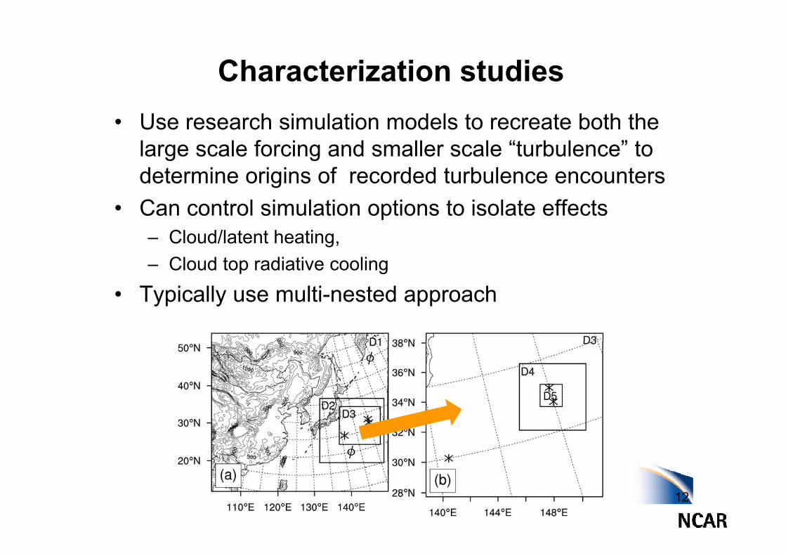
Characterization studies• Use research simulation models to recreate both the
large scale forcing and smaller scale “turbulence” tolarge scale forcing and smaller scale turbulence to determine origins of recorded turbulence encounters
• Can control simulation options to isolate effectsCan control simulation options to isolate effects– Cloud/latent heating, – Cloud top radiative cooling
• Typically use multi-nested approach
12

Simulations to identify relation of cirrus bands to turbulence*bands to turbulence*
*Knox et al. “Transverse cirrus bands in weather systems: a grand tour of an enduring enigma” Weather 2006

Example cirrus bands/turbulence 15 Nov 2011*
FL310
Forecasted turbulent areas
*Courtesy MelissaThomas DAL

Simulations of two cirrus bands cases
17 June 2005 Moderate and severe turbulence insitu edr measurements near Transverse (Radial) MCS Outflow Bands over central US
9 Sep 2010 : Moderate and severe turbulence reported in vicinity of mid-latitude cyclone over western
15
over central US- Trier & Sharman MWR 2009- Trier et al. JAS 2010
Pacific Ocean- Kim et al. submitted to MWR

Example 1. Out-of-cloud CIT near MCS*Observedturbulence
In situ edr + wind vectors
43 N
Note bands are transverse to wind vectors
43 N0905 UTC 16 June
40 N Model TKE
37 N
Courtesy UW CIMSS
*Trier and Sharman, MWR, 2009*Trier et al JAS 2010
ARWRF simulation ∆=3 kmCourtesy UW CIMSS

MCS CIT mechanism
With cloudNo cloud
No cloudWith cloud
• Strong vertical shear at flight levels due almost entirely to MCS outflow on north side• Vertical shear at flight levels on south side weaker because easterly outflow winds and shear are opposed by their westerly environmental (adiabatic) counterparts

Observations and WRF-Simulations of the17 June 2005 MCS Case 600m nest
Simulated Cloud Top Temperature (0950 UTC, t = 5.8 h ) Observed Turbulence @ 37 Kft (0936-0957 UTC) L=light M=ModerateIR Satellite at 0950 UTC 17 June 2005
17 June 2005 MCS Case – 600m nest
Observed Turbulence @ 37 Kft (0936-0957 UTC) L=light, M=ModerateIR Satellite at 0950 UTC 17 June 2005
Turbulence
UA776
Trier and Sharman (2009, Mon. Wea. Rev.) Observations and MCS-Scale SimulationsTrier et al. (2010, J. Atmos. Sci.) High-Resolution Simulation and Analysis of Radial Bands

m
4-hour Loop of Brightness Temperature, 12-km Moist Static Instability N < 0and 11.5-13-km Vertical Shear from 07-11 UTC 17 June with Dt = 10 min
2
Nor
th
Tb
East
• Anvil bands originate within zones of moist static instability• Bands are aligned along the anvil vertical shear vectorg g
Similar to horizontal convective rolls in boundary layer arising from thermal instability

Case 2: cirrus bands in mid-l tit d l 9 S 2010*
Control (CTL) Simulation No Cloud Radiative Feedback (NCR) Simulation
latitude cyclone 9 Sep 2010*Control (CTL) Simulation No Cloud Radiative Feedback (NCR) Simulation
xx
xx
x
Approximate Locations
x
Approximate Locations Approximate Locationsof Observed Turbulence
Approximate Locationsof Observed Turbulence
Domain 3= 3.3 km
Domain 3= 3.3 km
*J-H Kim submitted to MWR
Model-Derived Reflectivity and Sea-Level Pressure at 0300 UTC 9 Sep (t = 9 h)
500 kmJ-H Kim, submitted to MWR

Relation of wind shear vectors and
CTL at 2140 UTC 8 Sep 2010 (t = 3.67 h) CTL at 2340 UTC 8 Sep 2010 (t = 5.67 h)
stability to bands
Brightness Temperature, 11.75 km Moist Static Stability,200 kmBrightness Temperature, 11.75 km Moist Static Stability,10.75-12.75 km Wind Shear vectors
200 km

Brightness Temperature, and 11.75 km MSL Moist Static StabilityControl (CTL) Run No Cloud-Radiative Feedback (NCR) Run( ) ( )
2220 UTC 8 Sep(t = 4.33 h)
2310 UTC 8 Sep2310 UTC 8 Sep(t = 5.17 h)
200 km

Simulation of bands - summary
• Both cases show bands owe their existence to convective instability in anvil within background shear– MCS case: background shear mainly from upper-level
outflow– Pacific mid-latitude cyclone case: shear mainly from
j t tjet stream• Both have morphology akin to PBL rolls
Si b d i i t f ti l t bl i• Since bands originate from convectively unstable regions of anvil, it is not surprising that those areas are turbulentMCS case cloud top radiative cooling encourages• MCS case cloud-top radiative cooling encourages bands, in Pacific case it is crucial for bands
i23
Summary and future work• GTG
– Using an ensemble of turbulence diagnostics (GTG) instead of one diagnostic gives more robust performance
– Provides EDRTechnique can be used with any input NWP model– Technique can be used with any input NWP model
– Longer term goals• Forecast convective turbulence (CIT)• Provide probabilistic forecasts
– Use of in situ edr provides valuable verification source
• Numerical simulations– Use multi-nested approach to relate large scale to small scalesUse multi nested approach to relate large scale to small scales
for a variety of environments and turbulence sources– Helps understand turbulence genesis which may ultimately lead
to form lation of better diagnosticsto formulation of better diagnostics24