The Governance of Firms and Budget Constraint

The European Journal of Comparative Economics Vol. 16, no. 2, pp. 313-334

ISSN 1824-2979

http://dx.doi.org/10.25428/1824-2979/201902-313-334

How to overcome the crisis of the European growth potential? The role of the government*

Andrea Elekes, Péter Halmai**

Abstract

We suppose that the dramatic decline in the European output is more than a cyclical diversion from the potential output. We performed a medium term quantitative analysis combining data based on the production function and growth accounting approach. Our results show that the erosion of the European growth potential has been a longer latent process. It began well before the outbreak of the latest economic crisis. Simulations suggest that the recovery in the rate of potential growth can only be partial in the medium term and further erosion of the European growth potential can be expected in the longer term. Our analysis suggests that more attention should be focused on TFP growth. Therefore, the last part of our study tries to identify the factors that insure a more dynamic TFP growth and examine what the governments can do in order to increase productivity and overcome the crisis of the growth potential.1

JEL classification: O11, O41, O52, E17

Keywords: Potential growth, Growth accounting, European Union, Crisis, Total factor productivity

1. Introduction

In Europe, the pain caused by the current crisis has been particularly acute. We

suppose that the dramatic loss of the European output is more than a cyclical diversion

from the potential output. There were clear signs of the European growth potential

moderating for a long time. The previously latent elements began ‘to come to the

surface’ from the mid-1990s. At the same time, the financial and economic crisis that

began in 2008 has had significant impacts on the European growth potential too. The

impacts of the crisis and the slow recovery on the potential output are also reviewed in

our paper. These tendencies are examined in detail through the quantitative analysis. In

order to test our hypothesis we perform a medium term quantitative analysis combining

data based on the production function and growth accounting approach.

* The work was created in commission of the National University of Public Service under the priority

project KÖFOP-2.1.2-VEKOP-15-2016-00001 titled “Public Service Development Establishing Good Governance” in Ludovika Workshop.

** Corr. Member of the Hungarian Academy of Sciences; Professor, NUPS Faculty of International and European Studies, Department of Economics and International Economics.

1 Original manuscript submitted in September 2016.

EJCE, vol. 16, no. 2 (2019)

Available online at http://eaces.liuc.it

314

2. Methodology of the potential growth analysis

Potential growth is a cumulative measure showing the sustainable and non-

inflationary growth generating capacity of the economy. Growth rate of the potential

output reflects the steady-state economic dynamics (growth potential). Unlike the actual

growth rate it does not contain cyclical factors2.

The difference of the actual and the potential growth is the so called output gap, a

fundamental measure of business cycles. Instruments of the economic policy strongly

depend on the development of the output gap. However, it is very difficult to estimate

the value of the output gap. Potential growth cannot be directly observed, while data on

actual output could be updated from time to time.

The literature about growth is mainly dominated by articles discussing actual

growth trends. These trends reflect the business (and other kind of) cycles and they

provide important information. However, actual growth cannot permanently differ from

potential growth.

The European growth model and the performance of its sub-models can be

analysed also on the basis of potential growth. Potential growth can be analysed on the

one hand based on the past development path. There is an advantage in the ex post

analysis, namely that the degree of the actual output is known. At the same time,

potential growth can be measured through future projections too. Methodological

difficulties may occur in both cases.

Calculation (or estimation) of potential growth creates an opportunity to separate

structural development from cyclical development. There are different approaches.

Potential output can be estimated by trend outputs resulting from moving averages of

GDP time series and different filtering approaches. The most commonly used

application is the Hodrick-Prescott (HP) filter. It is a simple and transparent method.

Data with the highest frequency are utilized through the application of the filter3.

However, there are significant problems too. The method of HP filters does not have its

2 For details see e.g.: Denis et al. (2002), Denis et al. (2006), Hobza- McMorrow- Mourre (Eds.) (2009),

Basu - Fernald (2009), Steindel (2009), D’Auria et al. (2010), Havik et al. (2014).

3 We get the filtered series (i) from the original GDP series (ty ) with the help of the following algorithm:

21

2

11

2

1

T

t

ttttt

t

tyt

)(min

A, Elekes, P. Halmai, How to overcome the crisis of the European growth potential? The role of the government


315

roots in economic theories. Its features depend on the specific value of the smoothing

parameters4.

On the other hand, as all centered filters, they are loaded with endpoint

distortions, i.e. real time trend output estimates should be based on extrapolations of

GDP, possibly with subsequent revisions. Finally, similarly to other methods applied for

filtering GDP series, it cannot utilize information adequately to separate cyclical and

structural changes.

An alternative to simple data filtering is based on the supply side model of the

economy. Potential output is calculated in this case on the basis of a production

function, which is the result of the combination of contributions of production factors

and technological level. Compared with simple growth accounting, the production

function based approach of potential output is consistent with the balanced utilization

of the available resources (i.e.: oversupply or excess demand can be excluded).

However, although there are clear benefits relative to the HP filter, this approach

has its limits too. Its credibility depends on both the accessibility and the quality of data

on the contribution of production factors. This is a great challenge, especially as regards

the new member states of the EU.

We follow the growth accounting and production function approach in order to

calculate potential growth. This approach focuses mainly on the supply-side of the

economy, on the quantity and quality of labour, accumulation of capital and on the total

factor productivity as a driver of the output. The objective of this paper is to identify the

impacts of these drivers and to decompose the growth rate of the output based on their

impacts. In the production function approach potential growth can be calculated on the

basis of the development of labour and capital inputs and of the total factor

productivity. In order to apply the method, equilibrium rates of unemployment are

required too. These are provided by the NAIRU or NAWRU approaches5.

Under the framework of the production function approach, the determining

factors of the neoclassical growth model are taken into account. Recent growth (and

development) theories emphasize also the importance of further, mainly quality factors

4 The smoothing parameter generally equals 100 in case of yearly GDP data. This is the standard value

applied by the European Commission in trend output estimates.

5 NAWRU: Non-Accelerating Wage Rate of Unemployment.

EJCE, vol. 16, no. 2 (2019)


316

(innovation, geographical location, institutional system, macroeconomic policy etc.).6

The latter factors are important also in the ex post analyses. The uncertainty involved in

the ex ante analyses is, however, extremely high. In the production function approach

these factors have an impact through the development of the total factor productivity.

(The important qualitative factors of the economic system are taken into account in an

implicit way.) At the same time, it is difficult to quantify some of the factors mentioned.

That is why the ex ante analyses need to be carried out very cautiously. After all these

considerations, the production function approach can be applied in researches on

growth and development.

The production function and growth accounting approach has recently received

increasing attention in the literature. As regards to their long term application, studies,

e.g. on ageing in the European Union, are considered significant contributions to the

literature (e.g.: EC, 2011, 2012; Carone et al., 2006). As an example of the short term

approach and the mid-term extension of the growth accounting analysis we can mention

the database of the EU EPC Output Gaps Working Group (OGWG). (For their

methodology see Denis et al., 2002; Denis et al., 2006 and D’Auria et al., 2010.) The

methodology of the production function approach is described in the Appendix.

3. Impact of the crisis on the potential growth

After the outbreak of the financial and economic crisis the world economy was

week for years and the growth rate was well below the pre-crisis level7. Although the

significant decrease in the prices of oil and other raw materials and the monetary

expansion resulted in lower interest rates, they couldn’t meet the positive growth

expectations. Japan has been facing the problems of negative inflation for a long time,

this time even the euro zone was forced to take steps in order to ease the pressure of

negative inflation. The introduction of the quantitative easing was one of the most

important steps. It had certain positive impacts as regards the deflation risk

management, however, couldn’t succeed in increasing inflation to the targeted level.

Euro zone interest rate spreads decreased, share prices increased and the euro faced a

6 See e.g. the overall analysis of Jones and Romer (2011).

7 For details see e.g.: Furceri and Mourougane, 2009; Haugh et al., 2009; Hobza et al., 2009; Van den Noord et al., 2009; Reinhard and Rogoff, 2009; Crafts, 2012; Haltmaier, 2012; Ball, 2014.



317

huge level depreciation. High level of state and private sector debt played also an

important role in holding back growth8.

OECD outlooks (OECD, 2015, 2016) forecasted even in 2016 that growth rates

can’t reach their pre-crisis level either on the longer term. However, a growth in the

level of GDP can be seen for most of the EU countries from 2016-2017 onwards.

Growth can mainly be attributed to the improving investment environment (more

favourable financing costs, increasing profits and better business outlook)9.

The recovering growth rate had a high price: a relatively high rate of

unemployment, especially as regards youth and minority groups10. There are also several

other risks that may threaten the positive growth expectations: a sudden rise in financial

market volatility, increasing costs of borrowing money, higher level of international

trade protectionism and geopolitical risks.

Constant monetary adjustment and negative inflation expectations have resulted

in decreasing long term bond yields in several countries. Most of the euro zone short

and long term sovereign bonds e.g. have had negative yields. Long lasting low interest

rates may challenge several money market players. Continuous higher risk-taking

behaviour and search for greater yields may distort the evaluation of certain assets. The

low interest rate environment is a challenge for the long term investors, e.g. for weaker

European life insurance companies. Insurance companies must hold a significant part of

their capital in liquid investment assets so as to be able to perform in case of a sudden

payment need. Due to the low interest rates however, certain companies may not be

able to meet the compulsory capital requirements. As (with their investments) there’s a

strong link between insurance sector and the other players of the financial system, a

problem arising at the level of the insurance sector may spill-over to other players and

other sectors.

Technological development, more regulated markets and a change in the structure

of market players have resulted in a new microstructure of bond (or more precisely debt

type) markets. As regards the near future, stricter monetary policy can be expected.

Higher interest rates may result in more volatile asset prices and exchange rates. More

8 For more details see e.g.: World Bank, 2015.

9 For more details see e.g.: World Bank, 2018.

10 For more details see e.g.: OECD, 2018.

EJCE, vol. 16, no. 2 (2019)


318

limited bond market liquidity may have spill-over effects on other assets and markets as

well.

4. Development of potential growth and its factors (Quantitative

analysis11)

As credible, longer term time series are not available as for the EU27, we

examined the development of potential growth in the EU15 (member states of the EU

before 2004) and in the United States in our growth accounting analysis. Countries of

the EU15 were grouped into three groups. The six founding countries (DE, FR, IT, B,

NL, L) of the European Economic Community (EEC) belong to the group of

Founding 6 (F6). Economies of these countries have developed under the European

integration framework for more than 50 years. These countries represent the continental

European model (see Halmai – Vásáry, 2012). The “New” member states (N6) are the

(relatively) more developed countries that joined the European Communities or the

European Union in 1973 or in 1995: UK and IE representing the Anglo-Saxon model

and DK, FI and SE following the Scandinavian model and finally AT.12 The group of

the Mediterranean countries (M3) countries comprises Greece (EL), which joined the

Community in 1981 and the countries that have been member states since 1986 (ES and

PT). Members of this latter group follow the so called Mediterranean (economic

development) model.

Based on the above analysis we can summarize the main characteristics of the

growth models of the examined country groups.

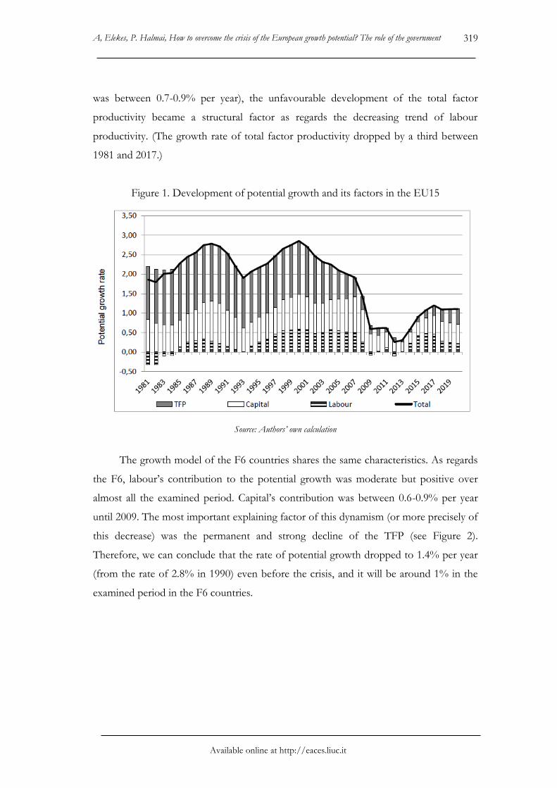
The potential growth rate of the EU15 has kept on decreasing since 1989 (see

Figure 1). This decrease can be explained by the development of the labour

productivity.13 Labour’s contribution was positive between 1995-2008, however the

growth rate of labour productivity has continuously decreased since 1993. As capital’s

contribution to the potential growth did not decrease significantly until 2009 (its rate

11 Analyses are based on the OGWG database as of 2017 Winter.

12 In the meantime the EU was enlarged by 10 new member states in 2004, by 2 in 2007 and by another one in 2013. These countries are considered to be the new member states nowadays. However, new member states refer to the above mentioned countries in this chapter.

13 In this analysis framework labour productivity’s impact on the potential growth is the sum of the capital’s and TFP’s contribution.



319

was between 0.7-0.9% per year), the unfavourable development of the total factor

productivity became a structural factor as regards the decreasing trend of labour

productivity. (The growth rate of total factor productivity dropped by a third between

1981 and 2017.)

Figure 1. Development of potential growth and its factors in the EU15

Source: Authors’ own calculation

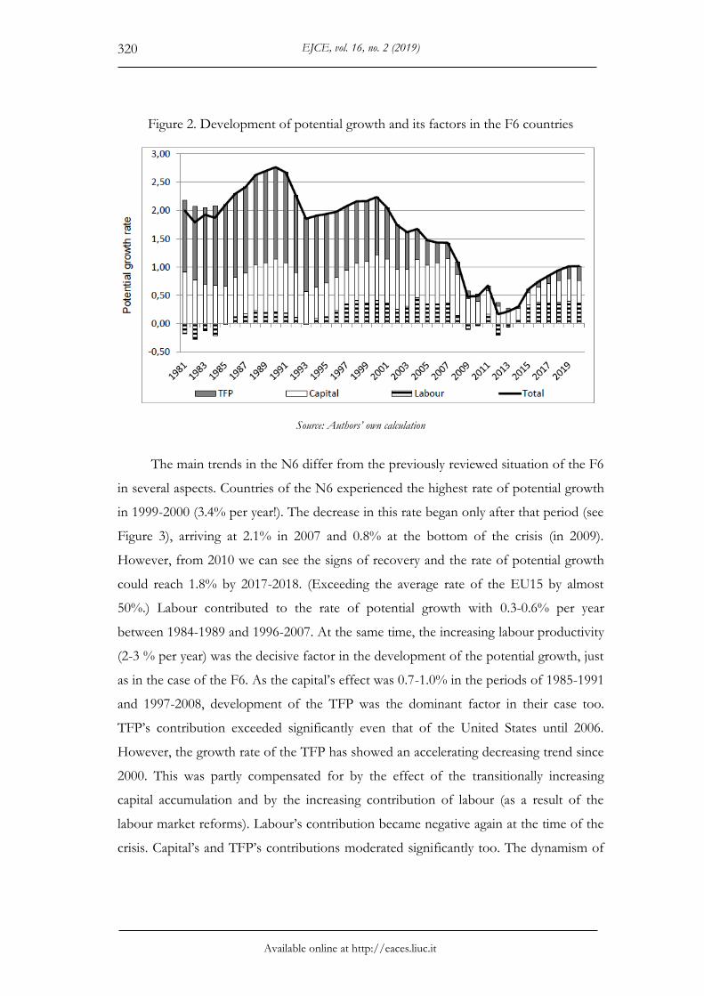
The growth model of the F6 countries shares the same characteristics. As regards

the F6, labour’s contribution to the potential growth was moderate but positive over

almost all the examined period. Capital’s contribution was between 0.6-0.9% per year

until 2009. The most important explaining factor of this dynamism (or more precisely of

this decrease) was the permanent and strong decline of the TFP (see Figure 2).

Therefore, we can conclude that the rate of potential growth dropped to 1.4% per year

(from the rate of 2.8% in 1990) even before the crisis, and it will be around 1% in the

examined period in the F6 countries.

EJCE, vol. 16, no. 2 (2019)


320

Figure 2. Development of potential growth and its factors in the F6 countries


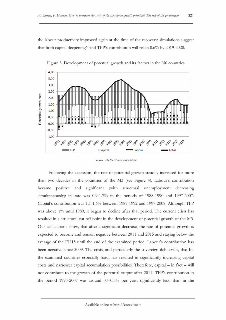
The main trends in the N6 differ from the previously reviewed situation of the F6

in several aspects. Countries of the N6 experienced the highest rate of potential growth

in 1999-2000 (3.4% per year!). The decrease in this rate began only after that period (see

Figure 3), arriving at 2.1% in 2007 and 0.8% at the bottom of the crisis (in 2009).

However, from 2010 we can see the signs of recovery and the rate of potential growth

could reach 1.8% by 2017-2018. (Exceeding the average rate of the EU15 by almost

50%.) Labour contributed to the rate of potential growth with 0.3-0.6% per year

between 1984-1989 and 1996-2007. At the same time, the increasing labour productivity

(2-3 % per year) was the decisive factor in the development of the potential growth, just

as in the case of the F6. As the capital’s effect was 0.7-1.0% in the periods of 1985-1991

and 1997-2008, development of the TFP was the dominant factor in their case too.

TFP’s contribution exceeded significantly even that of the United States until 2006.

However, the growth rate of the TFP has showed an accelerating decreasing trend since

2000. This was partly compensated for by the effect of the transitionally increasing

capital accumulation and by the increasing contribution of labour (as a result of the

labour market reforms). Labour’s contribution became negative again at the time of the

crisis. Capital’s and TFP’s contributions moderated significantly too. The dynamism of



321

the labour productivity improved again at the time of the recovery: simulations suggest

that both capital deepening’s and TFP’s contribution will reach 0.6% by 2019-2020.

Figure 3. Development of potential growth and its factors in the N6 countries


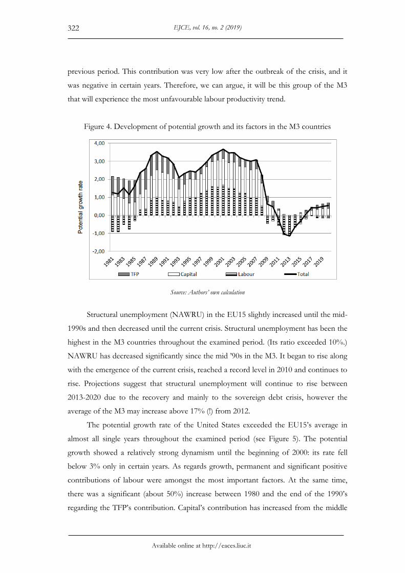
Following the accession, the rate of potential growth steadily increased for more

than two decades in the countries of the M3 (see Figure 4). Labour’s contribution

became positive and significant (with structural unemployment decreasing

simultaneously): its rate was 0.9-1.7% in the periods of 1988-1990 and 1997-2007.

Capital’s contribution was 1.1-1.6% between 1987-1992 and 1997-2008. Although TFP

was above 1% until 1989, it began to decline after that period. The current crisis has

resulted in a structural cut-off point in the development of potential growth of the M3.

Our calculations show, that after a significant decrease, the rate of potential growth is

expected to become and remain negative between 2011 and 2015 and staying below the

average of the EU15 until the end of the examined period. Labour’s contribution has

been negative since 2009. The crisis, and particularly the sovereign debt crisis, that hit

the examined countries especially hard, has resulted in significantly increasing capital

costs and narrower capital accumulation possibilities. Therefore, capital – in fact – will

not contribute to the growth of the potential output after 2011. TFP’s contribution in

the period 1995-2007 was around 0.4-0.5% per year, significantly less, than in the

EJCE, vol. 16, no. 2 (2019)


322

previous period. This contribution was very low after the outbreak of the crisis, and it

was negative in certain years. Therefore, we can argue, it will be this group of the M3

that will experience the most unfavourable labour productivity trend.

Figure 4. Development of potential growth and its factors in the M3 countries


Structural unemployment (NAWRU) in the EU15 slightly increased until the mid-

1990s and then decreased until the current crisis. Structural unemployment has been the

highest in the M3 countries throughout the examined period. (Its ratio exceeded 10%.)

NAWRU has decreased significantly since the mid ’90s in the M3. It began to rise along

with the emergence of the current crisis, reached a record level in 2010 and continues to

rise. Projections suggest that structural unemployment will continue to rise between

2013-2020 due to the recovery and mainly to the sovereign debt crisis, however the

average of the M3 may increase above 17% (!) from 2012.

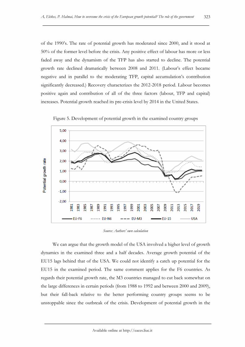
The potential growth rate of the United States exceeded the EU15’s average in

almost all single years throughout the examined period (see Figure 5). The potential

growth showed a relatively strong dynamism until the beginning of 2000: its rate fell

below 3% only in certain years. As regards growth, permanent and significant positive

contributions of labour were amongst the most important factors. At the same time,

there was a significant (about 50%) increase between 1980 and the end of the 1990’s

regarding the TFP’s contribution. Capital’s contribution has increased from the middle



323

of the 1990’s. The rate of potential growth has moderated since 2000, and it stood at

50% of the former level before the crisis. Any positive effect of labour has more or less

faded away and the dynamism of the TFP has also started to decline. The potential

growth rate declined dramatically between 2008 and 2011. (Labour’s effect became

negative and in parallel to the moderating TFP, capital accumulation’s contribution

significantly decreased.) Recovery characterizes the 2012-2018 period. Labour becomes

positive again and contribution of all of the three factors (labour, TFP and capital)

increases. Potential growth reached its pre-crisis level by 2014 in the United States.

Figure 5. Development of potential growth in the examined country groups


We can argue that the growth model of the USA involved a higher level of growth

dynamics in the examined three and a half decades. Average growth potential of the

EU15 lags behind that of the USA. We could not identify a catch up potential for the

EU15 in the examined period. The same comment applies for the F6 countries. As

regards their potential growth rate, the M3 countries managed to cut back somewhat on

the large differences in certain periods (from 1988 to 1992 and between 2000 and 2009),

but their fall-back relative to the better performing country groups seems to be

unstoppable since the outbreak of the crisis. Development of potential growth in the

EJCE, vol. 16, no. 2 (2019)


324

N6 countries however, is similar to that of the USA. (The growth of potential output

between 2001 and 2008 was even faster in the N6 countries than in the USA.) Labour

productivity, and particularly the dynamics of the total factor productivity, is the

decisive factors in accounting for the growth performance of the N6. The growth rate

of these factors exceeded the US levels up to 2006.

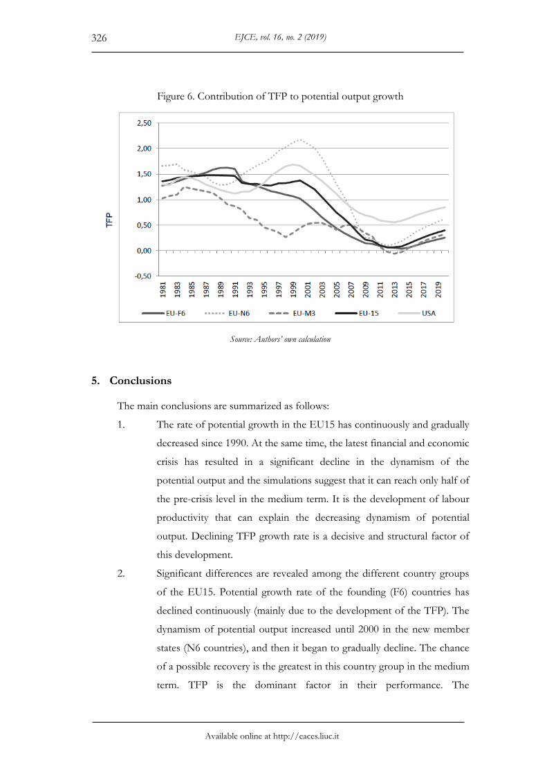
However, the USA had more robust structural characteristics (more favourable

total factor productivity above all)14 even before the outbreak of the crisis. Forecasted

demographic and TFP trends and investment and productivity dynamics are more

favourable than the forecasted trends for the EU15 and for the member states of the

euro zone. (See Figure 6.) Therefore, it is not surprising that the dynamics of the pre-

crisis growth potential can recover more or less in the United States, while it can reach

only the half of the pre-crisis level in the examined European countries.

14 The TFP gap, that has developed between the USA and the EU15 since the mid 1990s can mainly be

attributed to the differences in the intensity of the competitive environment, differences in innovation mechanisms and industrial structure, and to the different ratio of ICT and ICT dependent sectors. Revealing impact mechanisms of these factors requires further research.



325

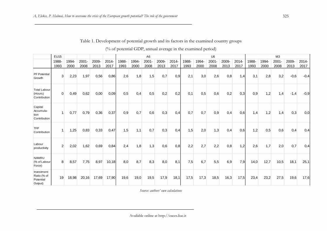
Table 1. Development of potential growth and its factors in the examined country groups

(% of potential GDP, annual average in the examined period)

Source: authors’ own calculations

EU15

1988-

1993

1994-

2000

2001-

2008

2009-

2013

2014-

2017

1988-

1993

1994-

2000

2001-

2008

2009-

2013

2014-

2017

1988-

1993

1994-

2000

2001-

2008

2009-

2013

2014-

2017

1988-

1993

1994-

2000

2001-

2008

2009-

2013

2014-

2017

PF Potential

Growth3 2,23 1,97 0,56 0,86 2,6 1,8 1,5 0,7 0,9 2,1 3,0 2,6 0,8 1,4 3,1 2,8 3,2 -0,6 -0,4

Total Labour

(Hours)

Contribution

0 0,49 0,62 0,00 0,09 0,5 0,4 0,5 0,2 0,2 0,1 0,5 0,6 0,2 0,3 0,9 1,2 1,4 -1,4 -0,9

Capital

Accumula-

tion

Contribution

1 0,77 0,79 0,36 0,37 0,9 0,7 0,6 0,3 0,4 0,7 0,7 0,9 0,4 0,6 1,4 1,2 1,4 0,3 0,0

TFP

Contribution1 1,25 0,83 0,33 0,47 1,5 1,1 0,7 0,3 0,4 1,5 2,0 1,3 0,4 0,6 1,2 0,5 0,6 0,4 0,4

Labour

productivity2 2,02 1,62 0,69 0,84 2,4 1,8 1,3 0,6 0,8 2,2 2,7 2,2 0,8 1,2 2,6 1,7 2,0 0,7 0,4

NAWRU

(% of Labour

Force)

8 8,57 7,75 8,97 10,18 8,0 8,7 8,3 8,0 8,1 7,5 6,7 5,5 6,9 7,9 14,0 12,7 10,5 18,1 25,1

Investment

Ratio (% of

Potential

Output)

19 18,98 20,16 17,69 17,90 19,6 19,0 19,5 17,9 18,1 17,5 17,3 18,5 16,3 17,5 23,4 23,2 27,5 19,6 17,6

A6 U6 M3

EJCE, vol. 16, no. 2 (2019)


326

Figure 6. Contribution of TFP to potential output growth


5. Conclusions

The main conclusions are summarized as follows:

1. The rate of potential growth in the EU15 has continuously and gradually

decreased since 1990. At the same time, the latest financial and economic

crisis has resulted in a significant decline in the dynamism of the

potential output and the simulations suggest that it can reach only half of

the pre-crisis level in the medium term. It is the development of labour

productivity that can explain the decreasing dynamism of potential

output. Declining TFP growth rate is a decisive and structural factor of

this development.

2. Significant differences are revealed among the different country groups

of the EU15. Potential growth rate of the founding (F6) countries has

declined continuously (mainly due to the development of the TFP). The

dynamism of potential output increased until 2000 in the new member

states (N6 countries), and then it began to gradually decline. The chance

of a possible recovery is the greatest in this country group in the medium

term. TFP is the dominant factor in their performance. The



327

Mediterranean (M3) countries followed a catch-up path until the

outbreak of the latest crisis. High structural unemployment was

successfully reduced and it became the decisive factor of potential

growth. From 2009 onwards very serious growth crises have developed

in these countries resulting in an extraordinary high level of the

NAWRU and a low level of investment and TFP.

3. In the long run the potential growth rate shows a declining trend both in

the USA and the EU15 countries. The TFP growth rate is much higher

in the USA from the middle of the 1990’s onwards than in the EU15 this

higher – although declining – dynamics is expected to last also in the

medium term. Further research is required to reveal the background of

the different dynamics.

4. All of the results suggest the same conclusion: source of the problems is

the decreasing dynamics of total factor productivity. If we want to stop

(or perhaps reverse) the declining trend of potential growth in the

European Union, we have to focus on the factors influencing the

development of the TFP.

5. There’s an increasing fear of a future (world) economic shock. Without

improvement and correcting the current problems a further erosion of

the European growth potential can be expected. This threatens not only

the development of the potential growth but may result in further

difficulties, e.g. market actors may lose their trust in the institutional

system, there may be an increasing trend of long term unemployment

etc.

What the national governments can do?

Globalisation and European Union itself has resulted in a reduced, limited

national sovereignty. However, national governments still have several possibilities to

reduce the negative effects of a possible future shock.

Fiscal policy e.g. can help to stabilize the economy at least in two ways. Automatic

stabilisers (income proportional tax systems, expenditures and social benefits) can

automatically increase the aggregate demand in case of a setback, while decrease it if

EJCE, vol. 16, no. 2 (2019)


328

there’s a boom in the economy. Another way to manage the possible negative effects of

a shock is to apply shock-specific instruments however, this may require an effective

fiscal stabilisation system.

Fiscal policy may have a decisive role in building up trust and influencing

aggregate demand. The place for maneuver is relatively limited, nonetheless fiscal policy

can effectively support the economic growth, decrease the potential risks and insure a

sustainable debt service. Infrastructural investments e.g. will increase the aggregate

demand on the short term and the potential output on the medium term. Relatively low

prices of raw materials (e.g. oil) may create an opportunity to change the energy-related

tax and support systems. These resources may compensate for the reduction in wage-

related taxes and expenses which may be necessary in order to enhance employment.

Re-allocation of these resources to education, health or infrastructural development may

also be an efficient way to improve productivity and resource allocation. (For details see

e.g.: IMF, 2015). Policy makers should be very responsive for these kinds of changes, as

low oil prices provide unique opportunity for unavoidable structural reforms that seem

to be almost impossible in times of higher oil prices.

As regards the long term unemployment, not only the above mentioned reduction

of labour costs but also the carefully chosen level of minimal wages and restructuring of

the unemployment benefit system (increasing the motivation in having a job) may help

to increase the labour demand of the economy. (For details see e.g.: Banerji et al., 2014.)

This is a serious concern for the public policy based on the traditional

employment model. Main objectives of these models is to help transition from

traditional forms of employment to less traditional ones. New models suggest that social

security systems, simplified registration and tax possibilities should cover all forms

employment. (For details see e.g.: ILO, 2015).

In order to avoid brain drain and outflow of the domestic labour it is essential to

create quality jobs and to enhance the diversification of the production capacity. (Risk

of a potential future shock is higher if growth performance of a country depends only

on a few export-oriented sectors.) The role of the economic policy is significant: anti-

cyclical economic policy ensures the adequate level of aggregate demand, certain kinds

of capital movement “limits” may be required to avoid problems caused by hot capital,

stabile and competitive exchange rate etc. (For details see e.g.: ILO, 2014.)



329

Strategic approach of the long term development requires a switch in the

economic policy: structural reforms that improve productivity may be more efficient

than the monetary and fiscal adjustment. Ageing societies also point in the direction of

productivity enhancing structural reforms, as the increasing labour market participation

and employment rate can only partly combat the decreasing level of labour supply.

(Japan e.g. bases its labour market strategy on robotics and digitalisation. Inward labour

migration can also be an alternative. And – although only on the longer term –

financially motivating parents to have more children may also be part of the solution.)

Structural reforms may be of special importance for those emerging, medium-income

countries that can no longer base their development on factors that characterised them

during the process of low to medium income countries (cheap labour, rapidly increasing

foreign direct investment in their export sectors etc.). Under these circumstances growth

will increasingly be dependent on a multi-factor productivity driven by accumulated

skills, knowledge, innovation and knowledge-based capital.

References

Banerji A. et al. (2014), ‘Youth Unemployment in Advanced Economies in Europe: Searching for Solutions’, IMF Staff Discussion Note. http://www.imf.org/external/pubs/ft/sdn/2014/sdn1411.pdf

Blanchard O., Summers L. H. (1989), ‘Hysteresis in Unemployment’, NBER Working Papers, 2035, National Bureau of Economic Research

Blanchard O., Wolfers J. (2000), ‘The Role of Shocks and Institutions in the Rise of European Unemployment: The Aggregate Evidence’, The Economic Journal, 110(462)

Basu S., Fernald J. G. (2009), ‘What Do We Know (And Not Know) About Potential Output?’, Federal Reserve Bank of St. Louis Review, July/August, 91(4), 187-213.

Carone G. et al. (2006), ‘Long-term labour productivity and GDP projections for the EU25 Member States: a production function framework’, European Economy Economic Papers, 253, European Commission (EC) Directorate General for Economic and Financial Affairs (DG ECFIN), Brussels

Cerra V., Saxena S. C. (2008), ‘Growth dynamics: the myth of economic recovery’, American Economic Review, 98(1).

Claessens S., Kose M. A., Terrones M. E. (2008), ‘What happens during recessions, crunches and busts’, IMF Working Paper, 8(274), International Monetary Fund

Claessens S., Kose M. A., Terrones M. E. (2011), ‘How do business and financial cycles interact’, IMF Working Paper, 11(88).

Crafts N. (2012), ‘Western Europe’s Growth Prospects: a Historical Perspective’, CAGE Online Working Paper Series, 2012(71), Coventry, UK, Department of Economics, University of Warwick.

EJCE, vol. 16, no. 2 (2019)


330

D'Auria F. et al. (2010), ‘The production function methodology for calculating potential growth rates and output gaps’, European Economy Economic Papers, 420, EC DG ECFIN, Brussels

Denis C. et al. (2006), ‘Calculating potential growth and output gaps – a revised production function approach’, European Economy Economic Papers, 247, EC DG ECFIN, Brussels

Denis C., Morrow K. Mc, Röger W. (2002), ‘Production function approach to calculating potential growth and output gaps – estimates for the EU Member States and the US’, European Economy Economic Papers, 176, EC DG ECFIN, Brussels

Elekes A., Halmai P. (2013), ‘Growth Model of the New Member States: Challenges and Prospects’, Intereconomics, 48(2), 124-130.

Furceri D., Zdzienicka A. (2012), ‘How costly are debt crises?’, Journal of International Money and Finance, 31(4), 726-742, June 2012.

EC (European Commission) (2014), ‘The 2015 Ageing Report: Underlying Assumptions and Projection Methodologies’, European Economy, 8, Brussels.

EC (2015), ‘The 2015 Ageing Report. Economic and budgetary projections for the 28 EU Member States (2013-2060)’, European Economy, 3, Brussels.

Furceri D., Mourougane A. (2009), ‘The effect of financial crises on potential output: new empirical evidence from OECD countries’, Organization for Economic Cooperation and Development ECO/WKP (2009)40

Gali J. (2015), ‘Hysteresis and the european unemployment problem revisited’, NBER Working Paper, 21430.

Halmai P., Vásáry V. (2012), ‘Convergence crisis: economic crisis and convergence in the European Union’, International Economics and Economic Policy, 9(3), 297-322, September, Springer.

Haugh D., Ollivaud P., Turner D. (2009), ‘The macroeconomic consequences of banking crisis in OECD countries’, OECD Working Paper, 683.

Havik K., et al. (2014), ‘The Production Function Methodology for Calculating Potential Growth Rates & Output Gaps, European Economy Economic Papers, 535, Brussels.

Hobza A., Mc Morrow K., Mourre G. (eds.) (2009), ‘Impact of the current economic and financial crisis on potential output’, European Economy Occasional Papers, 49, June 2009, EC DG ECFIN, Brussels.

ILO (2015), World employment and social outlook. The changing nature of jobs. http://www.ilo.org/wcmsp5/groups/public/---dgreports/---dcomm/---publ/documents/publication/wcms_368626.pdf

ILO (2014), World of Work Report 2014. Developing with jobs. http://www.ilo.org/wcmsp5/groups/public/---dgreports/---dcomm/documents/publication/wcms_243961.pdf

IMF (2015c), Fiscal Monitor – Now Is the Time: Fiscal Policies for Sustainable Growth. http://www.imf.org/external/pubs/ft/fm/2015/01/pdf/fm1501.pdf

Jones C., Romer P. (2011), ‘The New Kaldor Facts: Ideas, Institutions, Population, and Human Capital’, American Journal of Economics: Macroeconomics, 2(1), 224–224.

Jung E. (2014), ‘Misleading indicators’, The Daily Star, http://www.thedailystar.net/misleading-indicators-17216

Kurzweil R. (2005), The singularity is near: when humans trascend biology. Penguin Books Ltd, USA

Maktoum, Mohammed bin Rashid Al (2015), ‘Innovate or stagnate’, Project Syndicate, https://www.project-syndicate.org/commentary/government-corporate-innovation-by-mohammed-bin-rashid-al-maktoum-2015-02?barrier=accessreg

Mody A., Sandri D. (2012), ‘The Eurozone crisis: how banks and sovereigns came to be joined at the hip’, Economic Policy, 27(70), 199-230, April 2012.



331

OECD (2015), Economic Outlook, 1. http://www.keepeek.com/Digital-Asset-Management/oecd/economics/oecd-economic-outlook-volume-2015-issue-1_eco_outlook-v2015-1-en#page4

OECD (2016), Economic Outlook, https://read.oecd-ilibrary.org/economics/oecd-economic-outlook-volume-2016-issue-2_eco_outlook-v2016-2-en#page1

OECD (2018), Unemployment rate (indicator), doi: 10.1787/997c8750-en

Planas C., Roeger W., Rossi A. (2010), ‘Does capacity utilisation help estimating the TFP cycle?’, European Economy Economic Paper, 410.

Porter M. E., Heppelmann J. E. (2014), ‘How Smart, Connected Products Are Transforming Competition?’, Harvard Business Review, November 2014.

Reinhart C. M., Rogoff K. S. (2009), This time is different: eight centuries of financial folly, Princeton

Reinhart C. M., Rogoff K. S. (2011), ‘From financial crash to debt crisis’, American Economic Review, 101(5), 1676-1706, August;

Roubini N. (2016), ‘Has the global economic growth malaise become the 'new normal'?’, https://www.theguardian.com/business/2016/may/02/the-global-economic-growth-funk

Schumpeter J. A. (1934), The Theory of Economic Development: An Inquiry into Profits, Capital, Credit, Interest and the Business Cycle, Cambridge, Harvard University Press.

Solow R. M. (1956), ‘A Contribution to the Theory of Economic Growth’, The Quarterly Journal of Economics, 70(1), 65-94, February.

Steindel C. (2009), ‘Implications of the financial crisis for potential growth: Past, present, and future’, Staff Report, Federal Reserve Bank of New York, 408.

Van den Noord P. (ed.) (2009), ‘Economic crisis in Europe: causes, consequences and responses’, European Economy, 7, DG ECFIN, Brussels.

World Bank (2015), Global Economic Prospects. The Global Economy in Transition. A World Bank Group Flagship Report. http://www.worldbank.org/content/dam/Worldbank/GEP/GEP2015b/Global-Economic-Prospects-June-2015-Global-economy-in-transition.

World Bank (2017), Global Economic Prospects. A World Bank Group Flagship Report, http://www.worldbank.org

World Bank (2018), Global Economic Prospects. A World Bank Group Flagship Report, http://www.worldbank.org

World Economic Forum (WEF) (2017), The Global Competitiveness Report 2016–2017, http://www3.weforum.org/docs/GCR2016-2017/05FullReport/TheGlobalCompetitivenessReport2016-2017_FINAL.pdf

World Economic Forum (WEF) (2016), The Global Information Technology Report, http://www3.weforum.org/docs/GITR2016/WEF_GITR_Full_Report.pdf

EJCE, vol. 16, no. 2 (2019)


332

Appendix

The production function approach focuses on the supply potential of the

economy. In the framework of the production function approach potential GDP is the

result of the combination of factor inputs and technological level (total factor

productivity, TFP). While measuring potential output the cyclical factor is removed in

the case of labour and capital as well. (For details see D’Auria, 2010.)

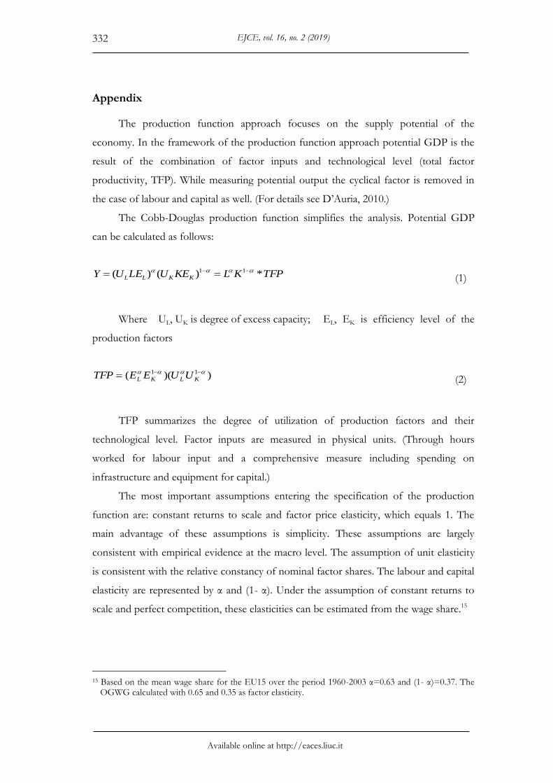
The Cobb-Douglas production function simplifies the analysis. Potential GDP

can be calculated as follows:

TFPKLKEULEUY KKLL *)()( 11 (1)

Where UL, UK is degree of excess capacity; EL, EK is efficiency level of the

production factors

))(( 11 KLKL UUEETFP (2)

TFP summarizes the degree of utilization of production factors and their

technological level. Factor inputs are measured in physical units. (Through hours

worked for labour input and a comprehensive measure including spending on

infrastructure and equipment for capital.)

The most important assumptions entering the specification of the production

function are: constant returns to scale and factor price elasticity, which equals 1. The

main advantage of these assumptions is simplicity. These assumptions are largely

consistent with empirical evidence at the macro level. The assumption of unit elasticity

is consistent with the relative constancy of nominal factor shares. The labour and capital

elasticity are represented by α and (1- α). Under the assumption of constant returns to

scale and perfect competition, these elasticities can be estimated from the wage share.15

15 Based on the mean wage share for the EU15 over the period 1960-2003 α=0.63 and (1- α)=0.37. The

OGWG calculated with 0.65 and 0.35 as factor elasticity.



333

While moving from actual to potential output the potential factor use (labour and

capital input) and the trend level (normal level) of efficiency of factor inputs need to be

defined.

Capital’s contribution to the potential output is given by the full utilization of

available capital in the economy. As capital stock is the indicator of full capacity, it is

unnecessary to smooth time series when applying the production function approach.

Series without smoothing tend to be more stable both for the EU and the USA. (For

details see D’Auria et al., 2010.) Investment shows significant fluctuation over the years.

Capital’s contributions however, are relatively stable. (Net investment is only a small

portion of capital stock in all of the years.)

It is more difficult to calculate the contribution of labour. Estimation of labour

input has several steps. The starting point is the maximum possible level, the

development of the working age population. The level of trend labour can be

determined from participation rates by applying HP filters. The next step is the

calculation of the trend unemployment in consistency with the NAWRU. Finally, we

can calculate the potential labour supply (number of trend work hours) multiplying

trend employment with average work hours. This approach generates relatively stable

potential employment series. At the same time, yearly development of the series may

strongly relate to long term demographic and labour market developments, to the actual

population of working age, to trend participation rate and to the development of the

structural unemployment.

As regards the production function approach potential output refers to the level

of output which can be produced with a “normal” level of efficiency of factor input.

This trend level efficiency level is measured by using a bivariate Kalman filter model

which is based on the link between the TFP cycle and the degree of capacity utilization

in the economy. (For details see Planas – Roeger – Rossi, 2010.) Normalizing the full

utilization of factor inputs, the potential output can be described as follows:

1)()( T

K

T

L

PP KEELY (3)

In the model described briefly the exogenous variables are as follows: population

of working age (POPW), smoothed participation rate (PARTS), investment ratio

EJCE, vol. 16, no. 2 (2019)


334

(expressed as percentage of potential GDP, IYPOT) structural unemployment (Non-

Accelerating Wage Rate of Unemployment - NAWRU), Kalman filtered Solow Residual

and trend average hours worked (HOURST). The endogenous variables are the

potential employment (LP), investment (I), capital stock (K) and the potential output.

(YPOT).

Potential employment for a given time period is determined as follows:

LPt=(POPWt*PARTSt*(1-NAWRUt)*HOURSTt

Development of investment and capital stock are determined by the following

equation:

It=IYPOTt*YPOTt and Kt=It+(1-dept)Kt-1,

where dept is depreciation rate of year t.

Based on all these the equation of the potential output can be described as

follows:

YPOT=LP 0.65 K 0.35 SRK (4)

We can determine the output gap with the following equation:

𝑌𝐺𝐴𝑃 = (𝑌 𝑌𝑃𝑂𝑇⁄ − 1)

The output estimates derived from production functions show the present output

capacity of the economy. Those enable a mid-term extension: they indicate the likely

development, if past trends were to persist.16 Projections for 2014-2018 in the OGWG

database can be considered technical extrapolations instead of forecasts.

16 In the mid-term extension the trend TFP, the NAWRU (Non-Accelerating Wage Rate of

Unemployment), the population of working age, participation rate changes, average hours worked, and the investment to potential GDP ratio are determined.

The Governance of Firms and Budget Constraint

Documents

Transcript of The Governance of Firms and Budget Constraint